Enhancing Numeric-SAM for Learning with Few Observations

Abstract

A significant challenge in applying planning technology to real-world problems lies in obtaining a planning model that accurately represents the problem’s dynamics. Numeric Safe Action Models Learning (N-SAM) is a recently proposed algorithm that addresses this challenge. It is an algorithm designed to learn the preconditions and effects of actions from observations in domains that may involve both discrete and continuous state variables. N-SAM has several attractive properties. It runs in polynomial time and is guaranteed to output an action model that is safe, in the sense that plans generated by it are applicable and will achieve their intended goals. To preserve this safety guarantee, N-SAM must observe a substantial number of examples for each action before it is included in the learned action model. We address this limitation of N-SAM and propose N-SAM^∗, an enhanced version of N-SAM that always returns an action model where every observed action is applicable at least in some state, even if it was only observed once. N-SAM^∗ does so without compromising the safety of the returned action model. We prove that N-SAM^∗ is optimal in terms of sample complexity compared to any other algorithm that guarantees safety. An empirical study on a set of benchmark domains shows that the action models returned by N-SAM^∗ enable solving significantly more problems compared to the action models returned by N-SAM.

1 Introduction

Automated domain-independent planning is a long-term goal of Artificial Intelligence (AI) research, intended to be a robust approach for sequential decision-making, equipped to address a wide spectrum of problems. While the domain-independent planning algorithms (planners) can be applied directly to different domains, they rely on having a domain model, written in some description language such as the Planning Domain Description Language (PDDL) (aeronautiques1998pddl) or its later extnsions (Fox and Long 2003; fox2002pddl+). A domain model in domain-independent planning includes the agent’s action model, i.e., which actions the agent can perform, the preconditions to apply them, and their effect on the environment. Manually formulating real-world problems within this framework is notoriously challenging. Consequently, there has been a substantial effort in developing algorithms to automatically learn PDDL domains in general and action models in particular, from observations (Cresswell and Gregory 2011; Aineto, Celorrio, and Onaindia 2019; Yang, Wu, and Jiang 2007; Juba, Le, and Stern 2021, inter alia).

Using learned action models for planning, however, is risky since the learned model is arguably less dependable than a human-made one. To address this concern, algorithms from the Safe Action Model (SAM) Learning family (Stern and Juba 2017; Juba, Le, and Stern 2021; Juba and Stern 2022; Argaman Mordoch 2023) learn safe action models, i.e., the return action models that, under certain conditions, are guaranteed to only allow plans that are applicable in the real environment. N-SAM, a recent addition to this line of research, is the first algorithm for learning safe action models in planning environments that can include continuous and discrete state variables. It runs in polynomial time and supports learning actions’ preconditions and effects that can be articulated as sets of polynomial inequalities and equations of some degree $k$.

To preserve safety, N-SAM does not include an observed action in the action model it returns before it has observed it multiple times in a sufficiently diverse set of states. Specifically, N-SAM learns the preconditions for an action $a$ by constructing an $n$-dimensional convex hull, where $n$ is a $k$-degree polynomial of the number of state variables. Consequently, N-SAM must observe action $a$ being applied in at least $n+1$ affinely independent states before it includes $a$ in the returned action model. In other words, if N-SAM lacks this initial set of observations, it deems the action inapplicable in every state. This limits the applicability of N-SAM, especially in large domains with many relevant state variables.

In this work, we propose N-SAM^∗, an enhanced version of N-SAM that overcomes this limitation. N-SAM^∗ includes every observed action in the action model it returns, even if it is only observed once, without compromising N-SAM’s safety requirement. This is achieved by computing for every action $a$ the subspace $D_{a}$ spanned by the states in which $a$ was observed, using a slightly modified version of the well-known Gram-Schmidt process. Then, we project all observations to $D_{a}$, and learn the preconditions and effects of $a$ on this possibly lower-dimensional subspace. The key observation is that an action can be safely applicable in a state $s$ if: 1) $s$ is linearly dependent in the observation states, i.e., it lies on $D_{a}$; and 2) $s$ is in the (possibly lower dimension) convex hull of the projections on $D_{a}$ of the observed states. We prove that N-SAM^∗ still runs in polynomial time, and the resulting action model is safe. Moreover, we prove that N-SAM^∗ is optimal in the sense that no other algorithm for learning safe numeric action models can deem an action applicable at some state if N-SAM^∗ deems it inapplicable. Finally, we empirically compare N-SAM and N-SAM^∗ on a set of benchmark domains, showing that N-SAM^∗ can indeed learn effective action models with fewer samples than N-SAM, enabling planners to solve more problems with the same amount of available data.

2 Preliminaries and Problem Definition

We focus on planning problems in domains where action outcomes are deterministic, states are fully observable and are described with discrete and continuous state variables. Such problems can be modeled using the PDDL2.1 (Fox and Long 2003) language. A domain is defined by a tuple $D=\left\langle F,X,A\right\rangle$ where $F$ is a finite set of Boolean variables, referred to as fluents; $X$ is a set of numeric variables referred to as functions; and $A$ is a set of actions. A state is the assignment of values to all variables in $F\cup X$. For a state variable $v\in F\cup X$, we denote by $s(v)$ the value assigned to $v$ in state $s$. Every action $a\in A$ is defined by a tuple $\left\langle\textit{name}(a),\textit{pre}(a),\textit{eff}(a)\right\rangle$ representing the action’s name, preconditions, and effects. The preconditions of action $a$ are a set of assignments over the Boolean fluents and a set of conditions over the functions. These conditions are of the form $(\xi,Rel,k)$ where $\xi$ is an arithmetic expression over $X$, $Rel\in\{\leq,<,=,>,\geq\}$, and $k$ is a number. The effects of action $a$, denoted $\textit{eff}(a)$, are a set of assignments over $F$ and $X$ representing how the state changes after applying $a$. An assignment over a Boolean fluent is either True or False. An assignment over a function $x\in X$ is a tuple of the form $\left\langle x,op,\xi\right\rangle$ where $\xi$ is a numeric expression over $X$, and $op$ is either increase (“+=”), decrease (“-=”), or assign (“:=”). The set of actions with their definitions is referred to as the action model of the domain. We say that an action $a$ is applicable in a state $s$ if $s$ satisfies $\textit{pre}(a)$. Applying $a$ in $s$, denoted $a(s)$, results in a state that differs from $s$ only according to the assignments in $\textit{eff}(a)$. A planning problem is defined by $\left\langle D,s_{0},G\right\rangle$ where $D$ is a domain, $s_{0}$ is the initial state, and $G$ are the problem goals. The problem goals $G$ are assignments of values to a subset of the Boolean fluents and a set of conditions over the numeric functions. A solution to a planning problem is a plan, i.e., a sequence of actions $\{a_{0},a_{1},...,a_{n}\}$ such that $a_{0}$ is applicable in $s_{0}$ and $a_{n}(a_{n-1}(...a_{0}(s_{0})...))$ results in a state $s_{G}$ in which $G$ is satisfied. A state transition is represented as a tuple $\left\langle s,a,s^{\prime}\right\rangle$, where $s$ denotes the state observed before the action’s execution, $a$ is an action, and $s^{\prime}$ is the result of applying $a$ in the state $s$, i.e., $a(s)$. The states $s$ and $s^{\prime}$ are commonly referred to as the pre-state and post-state, respectively.

Planning domains and problems are often defined in a lifted manner. That is, actions, fluents, and functions are parameterized, and their parameters may have types. Grounded actions, fluents, and functions are pairs of the form $\left\langle x,b_{x}\right\rangle$ where $x$ is the action, fluent, and function, respectively, and $b_{x}$ a function that maps parameters of $x$ to concrete objects. A state is the assignment of values to all grounded fluents and functions. A plan is a sequence of grounded actions. The preconditions and effects of an action in a lifted domain are parameter-bound fluents and functions. A parameter-bound fluent for an action $a$ is a pair $(f,b_{fa})$ where $f$ is a fluent and $b_{fa}$ is a function that maps every parameter of $f$ to a parameter in $a$. Parameter-bound functions are similarly defined. The lifted representation of the action fly in the Zenotravel domain is displayed in Figure 1, for example. The algorithms proposed in this work can learn lifted domains, and their implementations do so. However, we will describe our key algorithmic contribution assuming a grounded domain for ease of exposition.

Problem Definition

We consider a problem solver tasked with solving a numeric planning problem $\left\langle D=\left\langle F,X,A\right\rangle,s_{0},G\right\rangle$. The main challenge is that the problem solver does not receive explicit information about the set of actions $A$. Instead, it receives a collection of successful state transitions $\mathcal{O}$ extracted from a distribution of problems within the same domain $D$. A human operator, random exploration, or some other domain-specific process could have generated these observations. We assume the problem solver has full observability of these observation examples, signifying its awareness of the value of every variable in every state within every observation $o\in\mathcal{O}$, as well as knowledge of the name and parameters of every action in every observation $o\in\mathcal{O}$.

We also make the following assumptions. The actions’ preconditions over the numeric state variables are linear inequalities and The actions’ effects over the numeric state are linear functions of the numeric state variables. Later, we discuss how to relax this assumption and support polynomial preconditions and effects.

Action Model Learning

Different algorithms have been proposed for learning planning action models (Cresswell, McCluskey, and West 2013; Yang, Wu, and Jiang 2007; Aineto, Celorrio, and Onaindia 2019; Juba, Le, and Stern 2021). Some action-model learning algorithms, such as LOCM (Cresswell and Gregory 2011) and LOCM2 (Cresswell, McCluskey, and West 2013), analyze observed plan sequences, where each action appears as an action name and a vector containing the object names of the action’s arguments. Other action-model learning algorithms, such as FAMA (Aineto, Celorrio, and Onaindia 2019), can also utilize information about the states reached while executing plans in the domains. These algorithms only apply in classical planning domains and cannot be used to learn numeric domains. PlanMiner (Segura-Muros, Pérez, and Fernández-Olivares 2021) is a notable exception. It is an algorithm that learns numeric action models from partially known and potentially noisy observations. However, none of the presented algorithms guarantee that plans created with the learned action model are applicable in the real action model. The Safe Action Model Learning (SAM) learning framework (2017; 2021; 2022) addresses this gap by providing the following guarantee: the learned action model is safe in the sense that plans generated with it are guaranteed to be applicable and yield the predicted states.

N-SAM is an action model learning algorithm from the SAM learning framework designed to learn action models with Boolean and numeric state variables. N-SAM learns a lifted action model that includes all actions observed in the given observations $\mathcal{O}$. Since our work heavily depends on N-SAM, we briefly describe it here for completeness.

The N-SAM Algorithm

N-SAM starts by using SAM learning (Juba, Le, and Stern 2021) to learn the Boolean preconditions and effects of every observed action. Then, it creates numeric preconditions for every observed action $a$ by constructing a convex hull over the relevant numeric variables’ values observed in states before $a$ was applied. Finally, it creates numeric effects by solving a linear regression problem for every numeric variable that is part of the effects of that action. Next, we describe these steps in detail.

Learning Numeric Preconditions. For any action $a$, let $X(a)$ be the set of functions used in the preconditions and effects of $a$. If N-SAM does not know $X(a)$, it simply assumes it includes all functions. If $X(a)=\emptyset$, then $a$ does not have numeric preconditions. Otherwise, N-SAM creates a dataset of $|X(a)|$-dimensional points by iterating over every observed state transition $\left\langle s,a,s^{\prime}\right\rangle$ and extracting from $s$ the values for all the functions in $X(a)$. This dataset is denoted as $DB_{\textit{pre}(a)}$.

Then, N-SAM sets the preconditions of $a$ as the set of linear inequalities that form a convex hull of the points in $DB_{\textit{pre}(a)}$. Functions that are linearly dependent on other functions in every point in $DB_{\textit{pre}(a)}$ are extracted from the convex hull, and the linear dependency is translated into equality preconditions. Note that $DB_{\textit{pre}(a)}$ may not contain enough points to enable creating a convex hull. In such cases, N-SAM deems the action unsafe and does not include it in the returned action model.

Learning Numeric Effects. Under the linear effects assumption, the change in any variable $x\in X(a)$ is a linear combination of the variables in $X(a)$. Thus, N-SAM learns the effects of an action using standard linear regression.

In more detail, for every variable $x\in X(a)$ and given state transition $\left\langle s,a,s^{\prime}\right\rangle$ N-SAM creates an equation of the form :

$$s^{\prime}(x)=w_{0}+\sum_{x^{\prime}\in X(a)}w_{x^{\prime}}\cdot s(x^{\prime})$$ (1)

If the resulting system of linear equations contains fewer than $|X(a)|+1$ linearly independent equations, N-SAM considers $a$ unsafe and does not include it in the returned action model. Otherwise, it finds the unique solution to this set of equations and obtains the values of $w_{0}$ and $w_{x^{\prime}}$ for all $x^{\prime}\in X(a)$.

Safety. The N-SAM algorithm learns numeric action models with $\epsilon$-safety guarantees.

Definition 1 ($\epsilon$-Safe Action Model).

For $\epsilon\geq 0$, an action model $\hat{A}$ is $\epsilon$-safe w.r.t. a norm $\|\cdot\|$ in a planning domain $D=\left\langle F,X,A\right\rangle$ if for every $\hat{a}\in\hat{A}$ there exists $a\in A$ such that $\textit{name}(a)=\textit{name}(\hat{a})$ and for every state $s$: (1) if $\hat{a}$ is applicable in $s$ then so is $a$, and (2) if $\hat{a}$ is applicable in $s$ then applying it in $s$ results in a state that is $\epsilon$-close to that obtained by applying $a$ to $s$, i.e., $\|\hat{a}(s)-a(s)\|\leq\epsilon$.

Plans generated using an $\epsilon$-safe action models are safe in the sense that they execute as anticipated by the model, with a total error magnitude of at most $\epsilon$ times the plan length (by the triangle inequality). This small $\epsilon$ error is often unavoidable in practical scenarios due to factors like numerical accuracy issues and limited precision sensors.

Supporting Polynomial Domains

N-SAM supports learning action models with polynomials as preconditions and effects. For each possible monomial up to the desired degree, N-SAM creates a new numeric function with a value equal to the value of the corresponding monomial evaluated on the original numeric variables’ values. Then, it applies the same methods to the new and more extensive representation. We note that in polynomial domains, the number of linearly independent equations required to learn a unique solution to the equation system depends on the total number of monomials.

(:action fly

:parameters (?a - aircraft ?c1 - city ?c2 - city)

:precondition (and

(not (at ?a ?c1)) (at ?a ?c2)

(>= (fuel ?a) (* (distance ?c1 ?c2) (slow-burn ?a))))

:effect  (and (not (at ?a ?c1)) (at ?a ?c2)

(increase (total-fuel-used)

     (* (distance ?c1 ?c2) (slow-burn ?a)))

(decrease (fuel ?a)

     (* (distance ?c1 ?c2) (slow-burn ?a))))))

Figure 1: The fly action in the Zenotravel domain.

However, that given $n$ variables with degree of at most $m$ the number of monomials of degree $m$ is $\frac{(m+n-1)!}{m!(n-1)!}$. Thus, learning preconditions and effects that include high-degree polynomials may become intractable. For clarity, most of the following discussion will assume that the preconditions and effects are linear. However, applying N-SAM and N-SAM^∗ to domains with polynomial preconditions and effects is done in the same fashion as described above.

Limitations

N-SAM presents several appealing theoretical properties, but it has a critical limitation that manifests when the number of observations available for an action $a$ is small with respect to the size of $X(a)$ and $k$. If the maximal number of non-collinear points in $DB_{\textit{pre}(a)}$ is less than $|X(a)|+1$, constructing a convex hull becomes infeasible, and N-SAM cannot learn the preconditions of $a$. Furthermore, if the number of linearly independent equations constructed by N-SAM (Equation 1) is less than $|X(a)|+1$, no unique solution exists, and N-SAM cannot learn the effects of $a$. Consequently, $a$ will not be returned in the learned action model.

These restrictions hinder the algorithm’s performance since they require many samples to learn actions. This becomes highly noticeable in domains with many numeric variables. For example, consider the action fly of the Zenotravel domain presented in Figure 1. In this domain, eight functions are present, with preconditions and effects expressed through quadratic inequalities associated with these functions. Consequently, N-SAM creates a total of $\sum_{k=1}^{2}{8\choose 2}+1=37$ functions that correspond to all the monomials. As a result, N-SAM requires a minimum of 37 independent observations in which the fly action is applied to learn an initial action model.

3 The N-SAM^∗ Algorithm

This section presents N-SAM^∗, an improved version of N-SAM that overcomes the above-mentioned limitations. N-SAM^∗ includes in the action model it returns every action that was observed, even if it was only observed once.

N-SAM^∗ Overview

Let $m$ be the dimension of space spanned by $DB_{\textit{pre}(a)}$. Even if $m<X(a)$, it is still possible to project the observations in $DB_{\textit{pre}(a)}$ into an $m$-dimensional space, facilitating the construction of the convex hull and ensuring that for any state within that space, any solution of the effects’ system of equations yields the same effects. Figure 2(a) illustrates this concept. Three observations are given: $\mathbb{R}^{3}:(1,0,0),(0,1,0),(0,0,1)$. Since at least four points are needed to construct a convex hull in $\mathbb{R}^{3}$, N-SAM cannot learn an action model given these observations. However, as shown in Figure 2(b), these three observations can be projected to two-dimensional space, in which a convex hull (triangle) can be constructed. Since the numeric preconditions are conjunctions of linear inequalities, we know that every state that lies in the subspace spanned by $DB_{\textit{pre}(a)}$ and is within the convex hull created in that subspace must be applicable in the true action model. The N-SAM^∗ algorithm we introduce next follows this rationale.

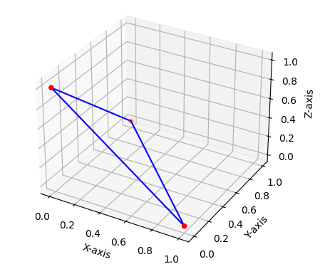
(a)

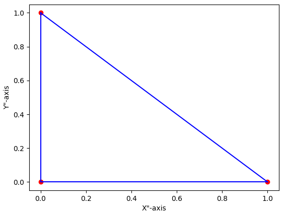
(b)

Figure 2: The points $(1,0,0),(0,1,0),(0,0,1)$. In Figure 2(a), they are displayed as 3-D points on the $\mathbb{R}^{3}$ space, and in Figure 2(b), they are displayed as projections on the 2-D plane.

Algorithm 1 lists the pseudo-code of N-SAM^∗. First, it learns the preconditions and effects of the Boolean variables, using the SAM Learning algorithm (Juba, Le, and Stern 2021). Then, for every action $a$ it creates two sets of vectors Base and CompBase. Base is an orthonormal basis for the subspace $D_{a}$, and CompBase is an orthonormal basis for the complementing subspace, i.e., the subspace that includes all points except those in $D_{a}$. Then, N-SAM^∗ projects all the states in $DB_{\textit{pre}}(a)$ where $a$ was observed to the possibly lower dimension subspace spanned by Base, and compute the convex hull of these projected states (stored in $CH_{\textit{proj}}$). Then, N-SAM^∗ uses $CH_{\textit{proj}}$ and $CompBase$ to define the preconditions of $a$. The effects are learned by using any linear regression method, as in N-SAM, but allowing it to return solutions even if they are not unique. We provide a comprehensive explanation of each component below.

Algorithm 1 The N-SAM^∗ Algorithm

1:Input: the observed transitions $\mathcal{O}$

2:Output: a safe action model.

3:for $a\in A$ do

4:     $\textit{pre}_{bool},\;\textit{eff}_{bool}\leftarrow$ Apply SAM learning

5:     $DB_{pre}(a)\leftarrow$ numeric states in $\mathcal{O}$ where $a$ was applied .

6:     $DB_{post}(a)\leftarrow$ numeric states in $\mathcal{O}$ after $a$ was applied.

7:for $a\in A$ do

8:     $S\leftarrow\{v_{i}-v_{0}|\forall v_{i}\in DB_{pre}(a)\}$

9:     $Base\leftarrow$ FindBase$(S)$

10:     $CompBase\leftarrow$ FindCompBase$(Base)$ s

11:     $CH_{proj}\leftarrow$ ConvexHull$(\{project(s,Base)|s\in S\})$

12:     $\textit{pre}_{X}(a)\leftarrow$ CreatePre($CH_{proj}$, $Base$, $CompBase$

13:     $\textit{eff}_{X}(a)\leftarrow$ Apply regression on $DB_{pre}(a)$ and $DB_{post}(a)$

14:return $(\textit{pre},\textit{eff})$

Projection to a Lower Dimension

Employing dimensionality reduction for learning preconditions and effects involves finding a basis for the lower dimensional subspace, projecting existing observations to this subspace, and determining whether a new observation lays in that subspace. To perform these steps, we first introduce the following auxiliary function, which is based on the classical Gram-Schmidt process (2013) and listed in Algorithm 2.

Algorithm 2 Gram-Schmidt for Planning

1:Function GS($points,Base$)

2:Output: Orthonormal base $B^{\prime}\perp Base$

3:$Vec\leftarrow Base$

4:$NVec\leftarrow\emptyset$

5:for $p\in points$ do

6:     $p_{proj}\leftarrow p-\sum_{v\in Vec}\frac{p\times v}{(\left\lVert v\right\rVert_{2})^{2}}\cdot v$

7:     if $|p_{proj}|>\epsilon$ then $\triangleright$ $\epsilon$ controls numeric accuracy

8:         $Vec\leftarrow Vec\cup\{p_{proj}\}$

9:         $NVec\leftarrow NVec\cup\{\frac{p_{proj}}{\left\lVert p_{proj}\right\rVert_{2}}\}$      

10:return $NVec$

The original Gram-Schmidt process (GSP) transforms a set of linearly independent vectors into an orthonormal set. Our auxiliary function includes two main changes to GSP. First, we initiate the GSP with an initial base (denoted as $Base$ in the input and line 3 of the algorithm). Consequently, the returned set would be orthogonal to the given base. Second, we only include vectors in the returned set if their projection with respect to all other points in the set is greater than some small $\epsilon$ (line 7). This allows us to relax the assumption of GSP that the input vectors are linearly independent.

Overall, the algorithm works as follows. It receives the points it uses as the input vectors, i.e., $points$, as well as the $Base$. The algorithm starts by assigning the input base to the variable $Vec$. $Vec$ represents the set of projected vectors that are all orthogonal to one another. Then, the algorithm sets $NVec$ to be an empty set. $NVec$ represents the orthonormal vectors created from $Vec$ by applying L2-normalization to them. The algorithm then iterates over the input vector points $p\in points$ and applies the Gram-Schmidt process to the point. If the projection of the point on the intermediate base is the zero vector (up to a distance of $\epsilon$ in each dimension), then it is spanned by the previous points and is ignored. Otherwise, it is added to $Vec$, and its normalized version is added to $NVec$. Finally, the algorithm outputs $NVec$ as an orthonormal set that is also orthogonal to the given base.

To project the observations to a lower dimensional space, N-SAM^∗ (Algorithm 1) shifts all observations so that the first observation becomes the new point of origin (line 8). Consequently, the first point is assured to be a zero-vector, serving as a linearly dependent reference for the remaining points. Subsequently, we calculate an orthonormal basis of the shifted data (line 10) using the enhanced Gram-Schmidt Process (GSP) outlined in Algorithm 2. Note that we do not provide the GSP with an initial base, so it returns an orthonormal basis for the given set of points.

After obtaining an orthonormal set of size $(m-1)$, the shifted observations can be projected into a $(m-1)$-dimensional space (line 10, argument of the ConvexHull call), this is done by taking the dot product of each shifted observation with the transposition of the orthonormal set. Consider, for example, a shifted observation $\mathbf{v}=[2,3,4]$, and assume that the orthonormal set returned from the GSP is:

$$\mathbf{u}_{1} =\left[\frac{1}{\sqrt{2}},\frac{1}{\sqrt{2}},0\right]\quad\mathbf{u}_{2}=\left[-\frac{1}{\sqrt{2}},\frac{1}{\sqrt{2}},0\right]$$

The transposition of the set is:

$$\begin{bmatrix}\frac{1}{\sqrt{2}}&\frac{1}{\sqrt{2}}&0\\ -\frac{1}{\sqrt{2}}&\frac{1}{\sqrt{2}}&0\end{bmatrix}^{T}=\begin{bmatrix}\frac{1}{\sqrt{2}}&-\frac{1}{\sqrt{2}}\\ \frac{1}{\sqrt{2}}&\frac{1}{\sqrt{2}}\\ 0&0\end{bmatrix}$$

The resulting observation is as follows:

$$\mathbf{v^{\prime}} =\begin{bmatrix}2&3&4\end{bmatrix}\begin{bmatrix}\frac{1}{\sqrt{2}}&\frac{1}{\sqrt{2}}\\ -\frac{1}{\sqrt{2}}&\frac{1}{\sqrt{2}}\\ 0&0\end{bmatrix}$$

$$=\begin{bmatrix}2\cdot\frac{1}{\sqrt{2}}+3\cdot\frac{1}{\sqrt{2}}+4\cdot 0\\ 2\cdot\left(-\frac{1}{\sqrt{2}}\right)+3\cdot\frac{1}{\sqrt{2}}+4\cdot 0\end{bmatrix}=\begin{bmatrix}2\sqrt{2}\\ \sqrt{2}\end{bmatrix}$$

Now, having transformed all observations into a lower dimension, we can proceed to learn the preconditions and effects in this reduced space.

Learning Numeric Preconditions

First, we need to show that transformed observations are sufficient for the purpose of computing a convex hull.

Lemma 3.1.

A convex hull can be constructed based on the set of transformed observations.

Proof.

Let $\mathcal{O}^{\prime}(a)$ be the set of transformed observations, where each observation has a dimension equal to the size of the orthonormal set $S$ returned by the GSP. After shifting the first observation to the origin, its projection, $o^{\prime}_{1}(a)$, becomes an $|S|$-dimensional zero vector. This ensures that $o^{\prime}_{1}(a)$ is linearly dependent on the other observations in $\mathcal{O}^{\prime}(a)$. Additionally, $S$ is an orthonormal set constructed based on the shifted observations.

Now, let $\mathcal{O}^{\prime\prime}(a)$ be a set of $|S|$ linearly independent observations along with $o^{\prime}_{1}(a)$. A set of points is affinely dependent if and only if subtracting one of them from the others results in a linearly dependent set (excluding the zero vector that results from subtracting the chosen point from itself). As subtracting $o^{\prime}_{1}(a)$ does not alter the other observations in $\mathcal{O}^{\prime\prime}(a)$, it is affinely independent.

Therefore, we have identified a subset of $\mathcal{O}^{\prime}(a)$ that contains $|S|+1$ affinely independent observations, each with $|S|$ dimensions. Consequently, it is possible to construct a convex hull based on the observations in $\mathcal{O}^{\prime}(a)$. ∎

The validity of line 11 in Algorithm 1 is ensured by Lemma 3.1. Mordoch et al.(2023) proved that an action $a$ is applicable from a state $s$ that lies within the convex hull of $a$ (Theorem 2 in their paper). Consequently, if a state $s^{\prime}$, resulting from applying the aforementioned transformation to $s$, resides within the convex hull, then action $a$ is applicable from $s^{\prime}$. However, it is essential to note that the transformation is guaranteed to be valid only for states within the span of the orthogonal set returned by the GSP. Our preconditions are required to address two aspects: 1) ensuring that the projected state resides within the convex hull, and 2) ensuring that the set of observations spans the state. To achieve 1), we must construct PDDL based on the facets of the convex hull, as described further below. To achieve 2), we construct the orthogonal set complementary to our base and ensure that $s^{\prime}$ is not spanned by that set.

To obtain a complementary orthogonal set, we once again leverage our extended GSP (Algorithm 2). This time, instead of providing the set of observations as input, we use the standard basis, denoted as ${e_{1},\dots,e_{n}}$, where each $e_{i}$ is an $|X(a)|$-dimensional vector with all values set to zero except for the $i$th dimension, which is set to one. Additionally, in this instance, the initial basis is not empty but is instead the orthogonal set $Base$ computed from the observations. Consequently, the GSP returns a set $CompBase$ that satisfies the following conditions: 1) it is orthogonal, 2) it is orthogonal to $Base$, and 3) the standard basis is linearly dependent in $CompBase\cup Base$. These conditions guarantee that $CompBase$ is indeed complementary to $Base$. To ensure that a given state $s$ is the span of $Base$, we can demonstrate that $s$ is orthogonal to $CompBase$. This can be achieved by adding preconditions that verify that the dot product of $s$ with every vector in $CompBase$ is zero.

Learning Effects

Argaman Mordoch (2023) proved (Theorem 3 in their paper) that, given the satisfaction of preconditions induced by the convex hull, the effects learned by solving the system of linear equations constructed using the set of observations, as described in Equation 1, are $\epsilon$-safe. In our context, there may not be enough equations to find a unique solution to the system. Nevertheless, any solution of the system is valid when the input state is linearly dependent on the set of observations. Consequently, since our preconditions ensure that the given state is linearly dependent on the observations, we can leverage linear regression algorithms to find some solution for the system and use it to learn $\epsilon$-safe effects. It’s important to note that N-SAM^∗ only allows solutions with an $R^{2}$ score of 1, indicating an exact solution to the system.

Overall, N-SAM^∗ ensures the acquisition of safe preconditions and $\epsilon$-safe effects, generating action models that are $\epsilon$-safe.

Translating the Preconditions to PDDL

The result of the GSP is a coefficient matrix that multiplies the observation points to create the lower dimensionality transformed points. Creating the actions’ preconditions in PDDL requires the projected points to be expressed in the original points’ space. Given a vector $v_{0}$ representing the first samples, the algorithm begins by subtracting every function $f_{i}$ from the corresponding value $v_{0}[i]$ (to match line 8). Then, each shifted function is multiplied by the result of our version of GSP, resulting in a set of factored shifted functions for each row in the GSP matrix. Finally, a linear combination is created from all the above-mentioned components. The result is the renamed functions in the original space that represent their projected values. Figure 3 presents an example of the process.

In Figure 4, we present the compiled output after applying the preconditions learning stage. Consider the following inequalities created by applying the convex hull algorithm on the resulting Gram-Schmidt base: $2x^{\prime}+3y^{\prime}\leq 3$ and $5x^{\prime}+4z^{\prime}\leq 17$. In this example, every function represents the result of the process present in Figure 3.

Next, consider applying the GSP with the standard basis and the projected base from the example (line 10 in Algorithm 1). The resulting conditions contain new functions that represent the subtraction of the original points by the first observation. We denote these functions as $x",y",z",w"$. One of the conditions obtained by applying this process is $0.76x"-0.29y"-0.51z"-0.25w"=0$. Translating this condition requires the algorithm to rename the functions using the subtraction operator for each new function.

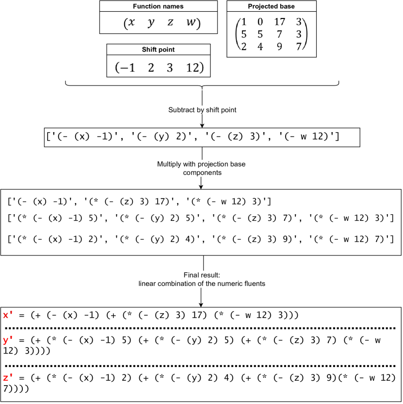
Figure 3: Example of the numeric variable renaming according to their projection on the Gram-Schmidt base.

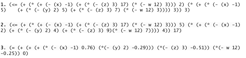
Figure 4: The translation of the convex hull and the equality conditions to PDDL.

Optimality

We now show that N-SAM^∗ is optimal by establishing that no alternative method for learning safe numeric action models can declare an action applicable at a certain state if N-SAM^∗ deems it inapplicable.

Theorem 3.2 (Optimality).

Let $M_{nsam^{*}}$ be the model generated by N-SAM^∗ given the set of observations $\mathcal{O}$, and let $M^{*}$ be the real action model. For every model $M$ that is safe w.r.t. $M^{*}$ and every state $s$ and action $a$, if $a$ is applicable in $s$ according to $M$ then it is also applicable in $s$ according to $M_{nsam^{*}}$.

Proof.

Let $a^{*}$ be an action that is not applicable in a state $s^{*}$ according to $M_{nsam^{*}}$. We will show that if $a^{*}$ is applicable in $s^{*}$ according to another action model $M$, then $M$ is not safe, from which the theorem follows immediately. If $a^{*}$ is not applicable in $s^{*}$ according to $M_{nsam^{*}}$, then $s^{*}$ violates one of the preconditions of $a^{*}$: if it is an equality precondition $b(s)=0$, then either $b(s^{*})>0$ or $b(s^{*})<0$. But notice, N-SAM^∗ only adds the equality precondition if $b(s^{\prime})=0$ for all $s^{\prime}$ appearing in the example observations. Thus, there exist action models that are consistent with the example observations in which $a^{*}$ has the precondition $b(s)\leq 0$ or $b(s)\geq 0$. Thus, $a$ is not applicable in some state $s^{*}$ for a possible action model; hence, $M$ is unsafe. Similarly, if we have $b(s^{*})>0$ for one of the convex hull faces $b(s)\leq 0$, then since all of the states $s^{\prime}$ appearing in example observations satisfied $b(s^{\prime})\leq 0$ (or else the convex hull would not have a face $b(s)\leq 0$) there is an action model in which $a^{*}$ has the precondition $b(s)\leq 0$ that is consistent with all of the example observations. Therefore, again, $M$ is not safe. ∎

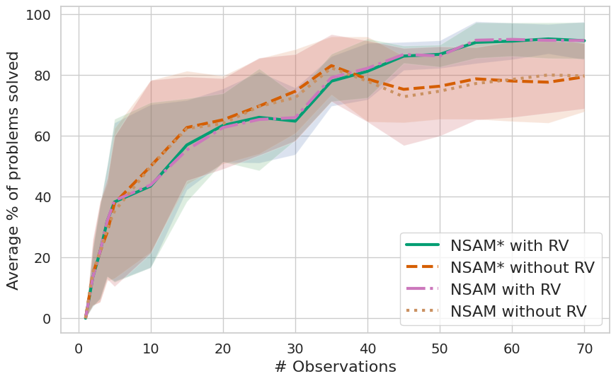
(a) Counters

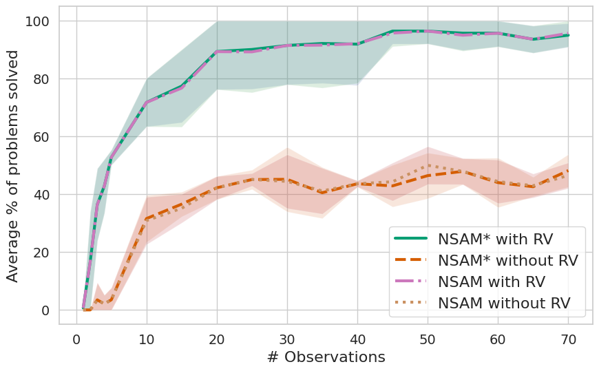
(b) Depots

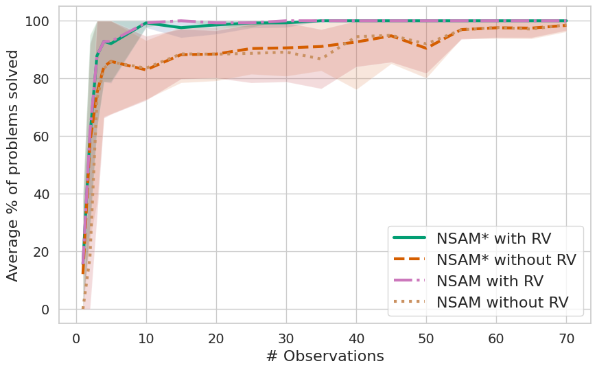
(c) Farmland

Figure 5: % test set problems solved for Counters, Depot, and Farmland.

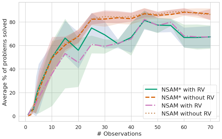
(a) Sailing

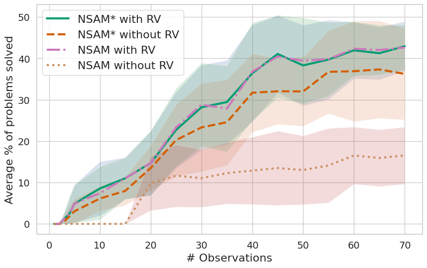
(b) Rovers

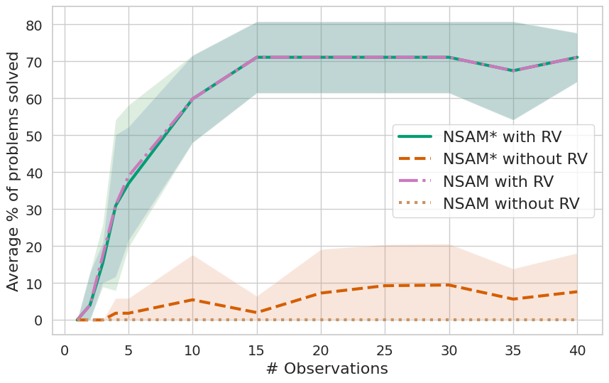
(c) Satellite

Figure 6: % test set problems solved for Sailing, Rovers, Satellite.

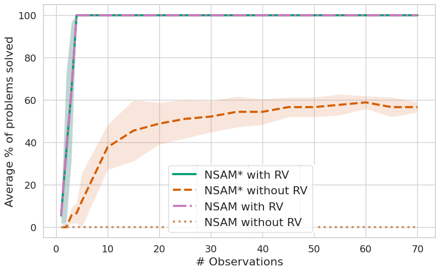
Figure 7: % test set problems solved for Driverlog.

4 Experimental Results

We implemented N-SAM^∗ and evaluated its performance on four classical domains from the 3rd International Planning Competition (IPC3) (Long and Fox 2003) namely - Depot, Driverlog, Rovers, and Satellite, as well as three domains used as testing benchmarks in IJCAI 2016  (Scala et al. 2017), namely - Farmland, Counters, and Sailing. Table  1 provides information about the experimented domains. The ‘Domain‘ column represents the name of the experimented domain, columns $|A|$, $|P|$, $|X|$ represent the number of actions, predicates, and numeric fluents in the domains. Finally, the columns $max\;\textit{pre}_{X}$ and $max\;\textit{eff}_{X}$ represent the maximal number of monomials relevant to the preconditions or the effects, respectively.

				$max$	$max$
Domain	$|A|$	$|P|$	$|X|$	$\textit{pre}_{X}$	$\textit{eff}_{X}$
Counters	4	0	3	3	2
Depot (IPC)	5	6	4	3	2
Driverlog (IPC)	6	6	4	0	2
Farmland	2	1	2	1	3
Sailing	8	1	3	3	2
Satellite (IPC)	5	8	6	2	3
Rovers (IPC)	10	26	2	1	2

Table 1: The domains used in the experiments.

Experimental Setup

We compared N-SAM^∗ with N-SAM. For each domain, we split the dataset into training and test sets, trained the algorithms on the observations in the training dataset, and evaluated the generated domains on the test set. All experiments were run on a CPU cluster with 64GB RAM memory limit.

We created our dataset by generating random problems using the IPC problem generator (Seipp, Torralba, and Hoffmann 2022). We also created our own generators for Farmland, Counters, and Sailing domains. We then used state-of-the-art numeric planners to solve the generated problems and the solved problems composed of our dataset. We conducted a 5-fold cross-validation process where, for each domain, the maximal number of input observations was set to 70 except for the Satellite domain, where the planner did not solve enough problems, resulting in only 40 observations in the training set.

We solved the test set problems using two solvers, Metric-FF (Hoffmann 2003) and ENHSP (Scala et al. 2016), both restricted to solving each planning problem within 300 seconds. The resulting plans were validated using VAL (Howey, Long, and Fox 2004). We only presented the results of the planner that, on average, had the best performance for all of the experimented algorithms in each domain, and the results were averaged over the five folds.

We experimented with two settings. First, we provided the algorithms with additional information, denoted as Relevant Variables (RV), representing the variables involved in each action’s preconditions. It is crucial to note that the algorithms do not possess further knowledge of the preconditions and effects; instead, they must learn them. Second, we let the algorithms run without providing the RV information. In this setting, the algorithms regard every possible variable as part of their actions’ preconditions, increasing the difficulty of the learning process.

In both N-SAM^∗ and N-SAM, the RV information only assists in learning once the algorithms observe enough samples to create $|X(a)|+1$ linearly independent equations with respect to Equation 1. Before observing $|X(a)|+1$ samples, the algorithms cannot guarantee that the observed effects correlate with the learned preconditions, i.e., those that contain fewer functions than those involved in learning the effects.

We also experimented with the polynomial IPC domains Zenotravel and Driverlog. However, our available computational resources were insufficient to accommodate the high memory and computational requirements imposed by the complexity of the domains.

Results

Our results are summarized in Figures 5,  6, and 7. The x-axis shows the number of given observations, and the y-axis is the average percent of the test set problems that were solved using the action models created by each algorithm. The results for the domains Driverlog, Depot, Farmland, and Satellite were achieved using ENHSP, and the rest of the domains’ results were achieved using the Metric-FF solver.

In Figure 5(b), we present the results obtained for the Depot domain. In this domain, the behavior of N-SAM^∗ and N-SAM is the same. When the algorithms receive the RV, there is an increase in the average solving rate of more than 40%. In the Farmland domain (Figure 5(c)), we observe a similar trend, although the difference between the algorithms using the RV and those that do not is smaller. Furthermore, the rates converge at the maximal number of observations.

For the Rovers, Satellite, and Driverlog domains (Figures 6(b), 6(c), 7), we observe the effectiveness of N-SAM^∗ compared to N-SAM. In these domains, when the algorithms do not receive the RV, the number of observations required to learn the action depends on the number of functions observed in the domain. Since the Rovers domain has only two lifted functions, N-SAM was able to learn the actions in the action model, resulting in test set problems being solved. On the other hand, both Driverlog and Satellite contain more numeric functions (four and six, respectively), resulting in N-SAM not learning the action model and thus not solving any test set problem. Since N-SAM^∗ does not have this restriction and can learn from as little as one observation, in the Driverlog domain, more than 50% of the test set problems were solved, and in the Sattelite domain, approximately 10% were solved.

We observe a different trend in the Counters domain (Figure 5(a)). In the interval between 10 and 40 observations, the algorithms not using the RV performed better than those that did. When inspecting the cause of the irregular behavior, we noticed that the domains learned by the algorithms using the RV were less complex than those created by the algorithm not using it. In these cases, the difference was caused either by an increased number of timeouts or by the fact that the planner was terminated due to increased resource consumption. This happened since less complex domains allow the planner to use more applicable actions, resulting in a larger action space. The larger action space results in more computational efforts for the planner, increasing the time and memory needed to solve planning problems.

In the Sailing domain (Figure 6(a), we observe similar trends to those observed in the Counters domain. Additionally, between 1 and 30 observations, N-SAM^∗ solves at least 10 percent more problems than N-SAM.

In conclusion, more complex domains show the efficiency of our new approach since fewer observations are required to learn action models that solve problems.

5 Conclusion and Future Work

This work discusses the N-SAM algorithm and its performance limitation; To create a convex hull for any action $a$, from a set of $m$ examples in $\mathbb{R}^{n}$, N-SAM requires at least $n+1$ affinely independent samples. If the input observations contain fewer independent samples, the algorithm considers the action unsafe, and it will always be inapplicable. To overcome this limitation, we presented N-SAM^∗, an enhancement to the N-SAM algorithm that can learn applicable action models with as little as one observation of every action. We provided theoretical guarantees to the algorithm, proving it is an optimal approach to learning numeric action models while still maintaining the safety property.

In future work, we intend to explore more polynomial domains that raise the learning process’s difficulty level. In addition, we intend to explore methods to automatically obtain the RV information to reduce the amount of human interaction with the learning process.

References

- Aineto, Celorrio, and Onaindia (2019) Aineto, D.; Celorrio, S. J.; and Onaindia, E. 2019. Learning action models with minimal observability. Artificial Intelligence, 275: 104–137.
- Argaman Mordoch (2023) Argaman Mordoch, B. J., Roni Stern. 2023. Learning Safe Numeric Action Models. In AAAI Conference on Artificial Intelligence (AAAI).
- Cresswell and Gregory (2011) Cresswell, S.; and Gregory, P. 2011. Generalised domain model acquisition from action traces. In International Conference on Automated Planning and Scheduling (ICAPS), 42–49.
- Cresswell, McCluskey, and West (2013) Cresswell, S.; McCluskey, T.; and West, M. 2013. Acquiring planning domain models using LOCM. The Knowledge Engineering Review, 28(2): 195–213.
- Fox and Long (2003) Fox, M.; and Long, D. 2003. PDDL2.1: An extension to PDDL for expressing temporal planning domains. Journal of Artificial Intelligence Research, 20: 61–124.
- Hoffmann (2003) Hoffmann, J. 2003. The Metric-FF Planning System: Translating “Ignoring Delete Lists” to Numeric State Variables. Journal of Artificial Intelligence Research, 20: 291–341.
- Howey, Long, and Fox (2004) Howey, R.; Long, D.; and Fox, M. 2004. VAL: Automatic plan validation, continuous effects and mixed initiative planning using PDDL. In 16th IEEE International Conference on Tools with Artificial Intelligence, 294–301. IEEE.
- Juba, Le, and Stern (2021) Juba, B.; Le, H. S.; and Stern, R. 2021. Safe Learning of Lifted Action Models. In International Conference on Principles of Knowledge Representation and Reasoning (KR), 379–389.
- Juba and Stern (2022) Juba, B.; and Stern, R. 2022. Learning Probably Approximately Complete and Safe Action Models for Stochastic Worlds. In AAAI Conference on Artificial Intelligence.
- Leon, Björck, and Gander (2013) Leon, S. J.; Björck, Å.; and Gander, W. 2013. Gram-Schmidt orthogonalization: 100 years and more. Numerical Linear Algebra with Applications, 20(3): 492–532.
- Long and Fox (2003) Long, D.; and Fox, M. 2003. The 3rd international planning competition: Results and analysis. Journal of Artificial Intelligence Research, 20: 1–59.
- Pitman (2012) Pitman, J. 2012. Probability. Springer Science & Business Media.
- Scala et al. (2017) Scala, E.; Haslum, P.; Magazzeni, D.; Thiébaux, S.; et al. 2017. Landmarks for Numeric Planning Problems. In International Joint Conference on Artificial Intelligence (IJCAI), 4384–4390.
- Scala et al. (2016) Scala, E.; Haslum, P.; Thiébaux, S.; and Ramirez, M. 2016. Interval-based relaxation for general numeric planning. In European Conference on Artificial Intelligence (ECAI), 655–663.
- Segura-Muros, Fernández-Olivares, and Pérez (2021) Segura-Muros, J. Á.; Fernández-Olivares, J.; and Pérez, R. 2021. Learning Numerical Action Models from Noisy Input Data. arXiv preprint arXiv:2111.04997.
- Segura-Muros, Pérez, and Fernández-Olivares (2021) Segura-Muros, J. Á.; Pérez, R.; and Fernández-Olivares, J. 2021. Discovering relational and numerical expressions from plan traces for learning action models. Applied Intelligence, 1–17.
- Seipp, Torralba, and Hoffmann (2022) Seipp, J.; Torralba, Á.; and Hoffmann, J. 2022. PDDL Generators. https://doi.org/10.5281/zenodo.6382173.
- Stern and Juba (2017) Stern, R.; and Juba, B. 2017. Efficient, Safe, and Probably Approximately Complete Learning of Action Models. In International Joint Conference on Artificial Intelligence (IJCAI), 4405–4411.
- Yang, Wu, and Jiang (2007) Yang, Q.; Wu, K.; and Jiang, Y. 2007. Learning action models from plan examples using weighted MAX-SAT. Artificial Intelligence, 171(2-3): 107–143.