DistilVPR: Cross-Modal Knowledge Distillation for Visual Place Recognition

Abstract

The utilization of multi-modal sensor data in visual place recognition (VPR) has demonstrated enhanced performance compared to single-modal counterparts. Nonetheless, integrating additional sensors comes with elevated costs and may not be feasible for systems that demand lightweight operation, thereby impacting the practical deployment of VPR. To address this issue, we resort to knowledge distillation, which empowers single-modal students to learn from cross-modal teachers without introducing additional sensors during inference. Despite the notable advancements achieved by current distillation approaches, the exploration of feature relationships remains an under-explored area. In order to tackle the challenge of cross-modal distillation in VPR, we present DistilVPR, a novel distillation pipeline for VPR. We propose leveraging feature relationships from multiple agents, including self-agents and cross-agents for teacher and student neural networks. Furthermore, we integrate various manifolds, characterized by different space curvatures for exploring feature relationships. This approach enhances the diversity of feature relationships, including Euclidean, spherical, and hyperbolic relationship modules, thereby enhancing the overall representational capacity. The experiments demonstrate that our proposed pipeline achieves state-of-the-art performance compared to other distillation baselines. We also conduct necessary ablation studies to show design effectiveness. The code is released at: https://github.com/sijieaaa/DistilVPR

1 Introduction

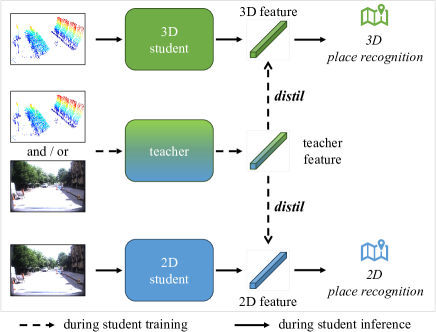
Figure 1: The pipeline of cross-modal KD to transfer knowledge from the cross-modal teacher to single-modal students.

Visual place recognition (VPR) serves as a foundational task in localization, aiming at identifying locations by comparing visual sensor data, such as camera images and LiDAR point clouds, to stored references in a database. This task finds application in diverse domains, including autonomous driving (Chen et al. 2023), precise positioning (Sarlin et al. 2019), and augmented reality (Sarlin et al. 2022).

Traditional VPR solutions rely on handcrafted features like Vector of Locally Aggregated Descriptor (VLAD) (Jégou et al. 2011) and Bag of Words (BoW) (Gálvez-López and Tardos 2012). These methods often fall short in challenging conditions including changing lighting, view distortions, and environmental perturbations due to their dependence on manual design.

The rise of deep learning has inspired data-driven VPR approaches that can tackle these challenges. NetVLAD (Arandjelovic et al. 2016) skillfully combines deep convolutional networks (CNNs) and traditional VLAD to enhance the robustness and efficacy of image scene feature extraction. This innovation paved the way for subsequent learning-based strategies. Addressing camera sensitivity to illumination, PointNetVLAD (Uy and Lee 2018) suggests utilizing point clouds from LiDARs which, unlike cameras, actively project laser beams to perceive surroundings, thus rendering them more resistant to lighting variations. Moreover, integrating data from multiple sensors can yield a more resilient and high-performing VPR model. In this vein, MinkLoc++ (Komorowski, Wysoczańska, and Trzcinski 2021) leverages both images and point clouds as inputs to achieve efficient multi-modal feature extraction, showcasing superiority over single-modal alternatives.

While integrating various sensors can elevate model performance, it also incurs additional expenses. Moreover, lightweight mobile systems might not support heavy sensors, such as LiDARs, making multi-modal sensors impractical.

Although using multiple sensors during inference is not favored, we can harness this cross-modal knowledge during student model training. This is where cross-modal knowledge distillation (KD) enters the picture. Specifically, in the student training phase, as depicted in Fig. 1, distinct modalities can be fed into the pre-trained teacher model. The extracted teacher features can then guide single-modal student models in learning superior features through additional supervision. During inference, student models can still rely on single-modal data, eliminating the need to accommodate multiple sensors.

Given the inconsistency in feature embedding across different modalities, directly compelling students to learn teacher features would be intricate. In contrast, the relational KD paradigm (Park et al. 2019), which delves into feature relationships, offers a more suitable approach to address this inconsistency. However, the vanilla relational KD solution only considers feature relationships in limited embedding spaces, and they restrict relationship computing within the same knowledge agents (i.e. either teacher-teacher relationships or student-student relationships). These limitations hinder the efficient transfer of knowledge from teachers to students.

To mitigate these issues, we propose DistilVPR, a novel cross-modal distillation pipeline for VPR. Our contributions can be summarized as follows:

• We present DistilVPR, a cross-modal KD solution uniquely tailored for VPR. This framework extends the scope of feature relationships, encompassing both self-agents and cross-agents to facilitate a more comprehensive exploration of knowledge. In addition, our approach performs feature embedding in multiple manifolds with diverse feature geodesic measurements, enhancing the construction of effective feature relationships

• Through extensive experiments, we showcase the remarkable performance of DistilVPR when compared to previous KD baselines. Our approach achieves state-of-the-art (SOTA) performance in the task of cross-modal distillation for VPR. Furthermore, we rigorously investigate our design through vital ablation studies, providing empirical evidence of the efficacy of our proposed methodology.

2 Related Work and Preliminary

In this section, we introduce related works and necessary manifold preliminaries.

2.1 Visual Place Recognition

NetVLAD (Arandjelovic et al. 2016) pioneers the combination of the traditional VLAD descriptor and the CNN to construct a learnable aggregation layer. Its success has paved the road for many VPR models. PointNetVLAD (Uy and Lee 2018) leverages point clouds instead of images to conduct place recognition. The point cloud features are extracted by PointNet (Qi et al. 2017) and then fed into a NetVLAD layer to produce the final global descriptor of the scene. MinkLoc3D (Komorowski 2021) is built based on a sparse 3D CNN for point cloud feature expression.

The aforementioned works use either images or point clouds for VPR. We now review approaches that take the multi-modal fusion strategy. Cues-Net (Oertel, Cieslewski, and Scaramuzza 2020) generates pseudo 3D point clouds from image sequences using Direct Sparse Odometry (DSO)(Engel, Koltun, and Cremers 2017). PIC-Net (Lu et al. 2020) transforms night images into the daytime style to reduce the impact of illumination perturbations on images. CORAL (Pan et al. 2021) projects the 3D point cloud using bird’s-eye-view (BEV) mapping, such that a 2D image backbone can be applied on both the point cloud branch and the image branch. MinkLoc++ (Komorowski, Wysoczańska, and Trzcinski 2021) follows the style of the MinkLoc3D series to achieve sparse 3D feature representation. The final global descriptor is concatenated with the 2D image descriptor and 3D point cloud descriptor. AdaFusion (Lai, Yin, and Scherer 2022) leverages a multi-scale attention module that hierarchically aggregates multi-modal features.

2.2 Knowledge Distillation

KD has emerged as a pivotal technique in model compression and multi-modal learning, enabling the transfer of knowledge from complex teacher models to compact or cross-modal student models. Vanilla KD (Hinton, Vinyals, and Dean 2015) first introduces the concept of KD to compress the knowledge from larger teacher models to smaller student models. RKD (Park et al. 2019) emphasizes the self-relationships present in the data samples of both teacher and student outputs. This approach serves as an implicit distillation solution, facilitating the transfer of the teacher’s knowledge to the student model. AFD (Ji, Heo, and Park 2021) employs an attention-based meta-network to acquire relative similarities among features and then employs these identified similarities to regulate the intensity of distillation for all feasible pairs. MKD (Jin, Wang, and Lin 2023) conducts prediction alignment at the instance of three different levels simultaneously, which include the instance, batch, and class levels.

There are also some other distillation works focusing on various tasks. 2DPass (Yan et al. 2022) employs an innovative approach to enhance semantic information extraction from multi-modal data with the integration of two key components: auxiliary modal fusion and multi-scale fusion-to-single distillation. LSD-Net (Peng et al. 2022) leverages dual distillation to transfer teacher patterns into students for lightweight VPR. EPC-Net (Hui et al. 2022) proposes ProxyConv, which is a lightweight module for local geometric feature aggregation. It uses a grouped VLAD network to form the global descriptors. To train its more lightweight version, the final feature is distilled from the larger teacher network to the smaller student network. CSD (Wu et al. 2022) represents a flexible framework for asymmetric similarity distillation to enhance the small query model for image retrieval. UniDistill (Zhou et al. 2023) digs into BEV object detection and leverages KD from features, relationships, and responses. LiDAR2Map (Wang et al. 2023b) presents an online camera-to-LiDAR distillation scheme to facilitate semantic information from images to point clouds for semantic map segmentation.

2.3 Manifold Preliminary

The concept of a manifold (Zhao et al. 2023; Wang et al. 2023a; She et al. 2023; Shi et al. 2023) serves as a generalization of surfaces in higher dimensions, extending the notion of well-behaved geometrical structures. A manifold $\mathcal{M}$ is a topological space that locally resembles the Euclidean space near each point $p\in\mathcal{M}$. For each point $p$, it is possible to establish a homeomorphism between a neighborhood of $p$ and the Euclidean space.

The tangent space $T_{p}\mathcal{M}$ at a point $p$ on $\mathcal{M}$ can be visualized as a hyperplane that provides the best approximation of $\mathcal{M}$ in the vicinity of $p$. Alternatively, $T_{p}\mathcal{M}$ is the space that encompasses all the possible directions of curves on $\mathcal{M}$ passing through $p$. The elements residing within $T_{p}\mathcal{M}$ are referred to as tangent vectors. Essentially, the tangent space $T_{p}\mathcal{M}$ characterizes the local linear approximation of $\mathcal{M}$ near the point $p$. It captures the intrinsic geometry of $\mathcal{M}$.

A metric tensor $g_{p}$ is an additional structure associated with each point $p$ on a manifold $\mathcal{M}$. By smoothly varying across $\mathcal{M}$, the metric tensor provides a consistent way to measure distances throughout the manifold. Given two points $p,q\in\mathcal{M}$, the geodesic distance $d(p,q)$ is obtained as the shortest length of curves that connect point $p$ and $q$.

3 Proposed Pipeline

In this section, we first provide the problem formulation. Then, we introduce the DistilVPR architecture in detail.

3.1 Problem Formulation

In this study, we address the challenge of cross-modal KD for VPR. We focus on a scenario where a pre-trained teacher model is provided, capable of processing images and/or point clouds as inputs for multi-modal VPR. The single-modal student models accept either image inputs or point cloud inputs. Our objective is to distill the teacher’s knowledge to the students, empowering them to acquire enhanced understanding during training. This, in turn, improves student performance during inference without the requirement for cross-modal sensors.

Specifically, we denote a batch of teacher outputs as $\mathbf{T}=\left\{\mathbf{t}_{i}\in\mathbb{R}^{C}\nonscript\,:\allowbreak\nonscript\,\mathopen{}i\in[N]\right\}$ and student outputs as $\mathbf{S}=\left\{\mathbf{s}_{i}\in\mathbb{R}^{C}\nonscript\,:\allowbreak\nonscript\,\mathopen{}i\in[N]\right\}$, with the batch size $N$ and the same output channel size $C$ .

3.2 Relational Distillation

There are typically two ways to conduct KD, including direct KD and relational KD. Direct KD is a straightforward way that directly applies sample-wise supervision by minimizing the loss

$$\mathcal{L}_{\rm{direct}}=\sum_{i\in[N]}\ell\left(\mathbf{t}_{i},\mathbf{s}_{i}\right),$$ (1)

where $\ell\left(\cdot\right)$ denotes the loss function. This approach pulls student embeddings towards teacher embeddings, which can be regarded as sample-wise supervision.

By contrast, relational KD does not apply explicit sample-wise supervision. Instead, it measures inter-sample relationships, which can be regarded as implicit knowledge. Relational KD is formed by minimizing

$$\mathcal{L}_{\rm{relationship}}=\sum_{i,j\in[N]}\ \ell\left(r\left(\mathbf{t}_{i},\mathbf{t}_{j}\right),\ r\left(\mathbf{s}_{i},\mathbf{s}_{j}\right)\ \right),$$ (2)

where $r(\cdot,\cdot)$ is the relational function to compute embedding distances.

Through our experiments, we have observed that compared with direct KD, relational KD is inherently a better choice for cross-modal KD in VPR for the following reasons. On one hand, in VPR, places are recognized by computing query-database similarity, where the training goal is to minimize the query-positive distance and maximize the query-negative distance. The relative feature relationships are more critical than the absolute feature embeddings, for which the relational KD scheme that explores relative embedding distance would be a more suitable solution for VPR. On the other hand, cross-modal features may have inherently different embedding patterns. Thus it would be intractable to force single-modal features to be embedded in the same space as multi-modal features using direct KD schemes. Based on these insights, we follow the relational KD scheme in 2 to design a more efficient cross-modal distillation solution.

3.3 Multi-agent Relationship

We generically call a teacher output $\mathbf{t}_{i}$ or student output $\mathbf{s}_{i}$ an agent. One limitation of the basic relational KD is that it confines the computation of relationships within the same type of agent, i.e., teacher-teacher $r(\mathbf{t}_{i},\mathbf{t}_{j})$ and student-student $r(\mathbf{s}_{i},\mathbf{s}_{j})$. Despite relational KD being able to achieve considerably better performance than direct KD counterparts, it lacks a more generalized consideration of the combination of different agents.

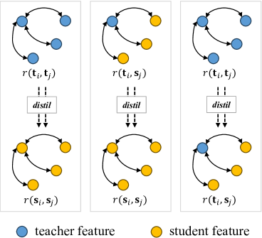
Figure 2: Three generalized relational KD schemes.

To generalize the combination of different agents, there are three scenarios for relationship computation as shown in Fig. 2. We expand 2 to further explore not only the self-agent relationships, $r(\mathbf{t}_{i},\mathbf{t}_{j})$ and $r(\mathbf{s}_{i},\mathbf{s}_{j})$, but also the cross-agent relationship, $r(\mathbf{t}_{i},\mathbf{s}_{j})$. Specifically, the three generalized relational KD losses are formulated as:

$$\mathcal{L}_{\rm{tt-ss}}=\sum_{i,j\in[N]}\ \ell\left(r\left(\mathbf{t}_{i},\mathbf{t}_{j}\right),\ r\left(\mathbf{s}_{i},\mathbf{s}_{j}\right)\ \right),$$ (3)

$$\mathcal{L}_{\rm{ts-ss}}=\sum_{i,j\in[N]}\ \ell\left(r\left(\mathbf{t}_{i},\mathbf{s}_{j}\right),\ r\left(\mathbf{s}_{i},\mathbf{s}_{j}\right)\ \right),$$ (4)

$$\mathcal{L}_{\rm{tt-ts}}=\sum_{i,j\in[N]}\ \ell\left(r\left(\mathbf{t}_{i},\mathbf{t}_{j}\right),\ r\left(\mathbf{t}_{i},\mathbf{s}_{j}\right)\ \right).$$ (5)

From above, 3 is the vanilla relational KD scheme in 2. By contrast, 4 and 5 are two additional schemes with 5 used in CSD (Wu et al. 2022). In the two schemes, cross-agent relationship $r\left(\mathbf{t}_{i},\mathbf{s}_{j}\right)$ bridges the gap between teacher features and student features. The additional information would contribute to a more effective KD process.

Comparing 4 and 5, we have empirically found that 4 generally outperforms 5, as seen in Table 4. This may be attributed to the fact that within the four variables in 5, only one pertains to the learnable student features, while the remaining three variables are associated with the fixed teacher features. Consequently, the optimal solution domain for minimizing 5 becomes constrained. For example, considering $r$ as the Euclidean distance function, the optimal solution is confined to a sphere. Similarly, this constraint could potentially elucidate why direct KD in 1 yields inferior results compared to relational KD, given that direct KD also involves only one variable for student features, resulting in the optimal solution domain that is a single point.

Based on these insights, we thus use 4 to compute cross-agent relationships, along with 3 for self-agent relationships. These distinct relationship patterns constitute the core components of our approach.

3.4 Multi-manifold Relationship

Since different modal features may not be embedded similarly, it becomes essential to adopt a more comprehensive metric for measuring agent relationships. Consequently, we introduce combined manifold spaces to augment the effectiveness of relational KD.

Different feature manifolds can be categorized based on their curvature. The Euclidean space represents the most prevalent manifold with zero curvature, while the spherical manifold exhibits positive curvature, and the hyperbolic manifold has negative curvature. By amalgamating multiple manifolds, we can facilitate features to possess more comprehensive embedding relationships by leveraging distinct geodesic distances.

Euclidean Relationship.

The Euclidean space serves as a prominent example of a flat manifold, exhibiting zero curvature across all points. Within Euclidean space, the calculation of the geodesic distance between any two points is given by the conventional Euclidean distance formula. The distance $d_{\rm{euc}}$ is the straight-line distance between two points $\mathbf{x},\mathbf{y}$ in a Cartesian coordinate system given by

$$d_{\rm{euc}}\left(\mathbf{x},\mathbf{y}\right)=\lVert\mathbf{x}-\mathbf{y}\rVert,$$ (6)

where $\lVert\cdot\rVert$ denotes the $\mathcal{L}_{2}$ norm.

In our work, the Euclidean distance yields the Euclidean-based losses as:

$$\mathcal{L}^{\rm{euc}}_{\rm{tt-ss}}=\sum_{i,j\in[N]}\ell\left(\ d_{\rm{euc}}\left(\mathbf{t}_{i},\mathbf{t}_{j}\right),\ d_{\rm{euc}}\left(\mathbf{s}_{i},\mathbf{s}_{j}\right)\ \right),$$ (7)

$$\mathcal{L}^{\rm{euc}}_{\rm{ts-ss}}=\sum_{i,j\in[N]}\ell\left(\ d_{\rm{euc}}\left(\mathbf{t}_{i},\mathbf{s}_{j}\right),\ d_{\rm{euc}}\left(\mathbf{s}_{i},\mathbf{s}_{j}\right)\ \right).$$ (8)

Spherical Relationship.

The second relationship we consider is the spherical relationship. In contrast to Euclidean space, the spherical manifold displays a distinct characteristic by possessing a constant positive curvature. The geodesic distance between two points is calculated based on the angular separation between the points and the radius of the sphere. Following previous works (Zhou et al. 2023; Hou et al. 2022), we adopt the cosine distance to explore the spherical-based relationship, which is given by

$$d_{\rm{cos}}(\mathbf{x},\mathbf{y})=\frac{\langle\mathbf{x},\mathbf{y}\rangle}{\lVert\mathbf{x}\rVert\lVert\mathbf{y}\rVert},$$ (9)

where $\langle\cdot,\cdot\rangle$ denotes the inner product.

Then we incorporate the cosine distance as the second consideration to explore positive-curvature relationships, and the losses are formulated as:

$$\mathcal{L}^{\rm{cos}}_{\rm{tt-ss}}=\sum_{i,j\in[N]}\ell\left(d_{\rm{cos}}(\mathbf{t}_{i},\mathbf{t}_{j}),d_{\rm{cos}}(\mathbf{s}_{i},\mathbf{s}_{j})\right),$$ (10)

$$\mathcal{L}^{\rm{cos}}_{\rm{ts-ss}}=\sum_{i,j\in[N]}\ell\left(d_{\rm{cos}}(\mathbf{t}_{i},\mathbf{s}_{j}),d_{\rm{cos}}(\mathbf{s}_{i},\mathbf{s}_{j})\right).$$ (11)

Hyperbolic Relationship.

A comprehensive relationship evaluation would benefit more from various feature pattern exploration of KD agents, and it can thus contribute to more effective KD from the teacher to the cross-modal student. However, the above two measurements explore feature relationships in either zero-curvature or positive-curvature manifolds as in RKD (Park et al. 2019). There is a lack of consideration of relationships in negative curvature manifolds, which would result in insufficient KD. To this end, we introduce the third relationship based on the negative curvature manifold.

In Riemannian geometry, the hyperbolic space is defined as the Riemannian manifold with constant negative curvature. The Poincaré ball is the most common conformal model of hyperbolic geometry. It has been used to embed features in various tasks (Tifrea, Bécigneul, and Ganea 2018; Liu, Nickel, and Kiela 2019; Wang et al. 2023a). The $n$-dimensional Poincaré ball is defined on $\mathbb{D}_{c}^{n}=\left\{\mathbf{p}\in\mathbb{R}^{n}\nonscript\,:\allowbreak\nonscript\,\mathopen{}c\lVert\mathbf{p}\rVert<1\right\}$ with curvature $-c^{2}$. The Poincaré ball is equipped with a constant metric tensor $\mathbf{g}=\lambda^{2}_{c}\mathbf{I}^{n}$, where $\lambda_{c}=\frac{2}{1-c\lVert\mathbf{p}\rVert^{2}}$ is the conformal factor.

Given a pair $\mathbf{p},\mathbf{q}\in\mathbb{D}_{c}^{n}$, the mobius addition $\oplus_{c}$ is defined as:

$$\mathbf{p}\oplus_{c}\mathbf{q}=\frac{\left(1+2c\langle\mathbf{p},\mathbf{q}\rangle+c\lVert\mathbf{q}\rVert^{2}\right)\mathbf{p}+\left(1-c\lVert\mathbf{p}\rVert^{2}\right)\mathbf{q}}{1+2c\langle\mathbf{p},\mathbf{q}\rangle+c^{2}\lVert\mathbf{p}\rVert^{2}\lVert\mathbf{q}\rVert^{2}}.$$ (12)

For a fixed base point $\mathbf{z}\in\mathbb{D}_{c}^{n}$, the exponential mapping function $\exp_{\mathbf{z}}^{c}:\mathbb{R}^{n}\rightarrow\mathbb{D}_{c}^{n}$ maps points from the tangent Euclidean space to the hyperbolic space:

$$\exp_{\mathbf{z}}^{c}(\mathbf{v})=\mathbf{z}\oplus_{c}\left(\tanh\left(\sqrt{c}\frac{\lambda_{c}\lVert\mathbf{v}\rVert}{2}\right)\frac{\mathbf{v}}{\sqrt{c}\lVert\mathbf{v}\rVert}\right).$$ (13)

By setting the origin as the fixed base point, the exponential map can be simplified as

$$\exp^{c}_{0}(\mathbf{v})=\tanh\left(\sqrt{c}\lVert\mathbf{v}\rVert\right)\frac{\mathbf{v}}{\sqrt{c}\lVert\mathbf{v}\rVert}.$$ (14)

After exponential mapping, the geodesic distance in the hyperbolic manifold (hyperbolic distance) can be obtained as

$$d_{\rm{hyp}}(\mathbf{p},\mathbf{q})=\frac{2}{\sqrt{c}}\operatorname{arctanh}\left(\sqrt{c}\lVert-\mathbf{p}\oplus_{c}\mathbf{q}\rVert\right).$$ (15)

In our work, we embed both teacher outputs and student outputs in the Poincaré ball, and the hyperbolic losses are computed as:

$$\mathcal{L}_{\rm{tt-ss}}^{\rm{hyp}}=\sum_{i,j\in[N]}\ell\left(\ d_{\rm{hyp}}\left(\mathbf{t}_{i}^{\rm{hyp}},\mathbf{t}_{j}^{\rm{hyp}}\right),d_{\rm{hyp}}\left(\mathbf{s}_{i}^{\rm{hyp}},\mathbf{s}_{j}^{\rm{hyp}}\right)\ \right),$$ (16)

$$\mathcal{L}_{\rm{ts-ss}}^{\rm{hyp}}=\sum_{i,j\in[N]}\ell\left(\ d_{\rm{hyp}}\left(\mathbf{t}_{i}^{\rm{hyp}},\mathbf{s}_{j}^{\rm{hyp}}\right),d_{\rm{hyp}}\left(\mathbf{s}_{i}^{\rm{hyp}},\mathbf{s}_{j}^{\rm{hyp}}\right)\ \right),$$ (17)

where $\mathbf{t}_{i}^{\rm{hyp}}=\rm{exp}^{c}_{0}(\mathbf{t}_{i})$ and $\mathbf{s}_{i}^{\rm{hyp}}=\rm{exp}^{c}_{0}(\mathbf{s}_{i})$ are hyperbolic teacher and student embeddings, respectively.

3.5 Overall Loss Function

Finally, we combine the insights from multiple agents and multiple manifolds to construct our distillation pipeline. Specifically, we first formulate two distillation losses, including the self-agent distillation loss $\mathcal{L}_{\rm{KD-S}}$ and the cross-agent distillation loss $\mathcal{L}_{\rm{KD-C}}$ respectively as:

$$\mathcal{L}_{\rm{KD-S}}=\mathcal{L}_{\rm{tt-ss}}^{\rm{euc}}+\mathcal{L}_{\rm{tt-ss}}^{\rm{cos}}+\mathcal{L}_{\rm{tt-ss}}^{\rm{hyp}},$$ (18)

$$\mathcal{L}_{\rm{KD-C}}=\mathcal{L}_{\rm{ts-ss}}^{\rm{euc}}+\mathcal{L}_{\rm{ts-ss}}^{\rm{cos}}+\mathcal{L}_{\rm{ts-ss}}^{\rm{hyp}}.$$ (19)

Subsequently, with weight hyperparameters $\lambda_{\rm{S}},\lambda_{\rm{C}}$ and the triplet loss as the VPR task loss $\mathcal{L}_{\rm{task}}$, we propose three different overall losses. They are denoted as DistilVPR-S, DistilVPR-C, and DistilVPR-SC, respectively:

$$\mathcal{L}_{\rm{DistilVPR-S}}=\mathcal{L}_{\rm{task}}+\lambda_{\rm{S}}\mathcal{L}_{\rm{KD-S}},$$ (20)

$$\mathcal{L}_{\rm{DistilVPR-C}}=\mathcal{L}_{\rm{task}}+\lambda_{\rm{C}}\mathcal{L}_{\rm{KD-C}},$$ (21)

$$\mathcal{L}_{\rm{DistilVPR-SC}}=\mathcal{L}_{\rm{task}}+\lambda_{\rm{S}}\mathcal{L}_{\rm{KD-S}}+\lambda_{\rm{C}}\mathcal{L}_{\rm{KD-C}}.$$ (22)

4 Experiments

In this section, we conduct experiments to compare DistilVPR defined in 20, 21 and 22 with other KD baselines. We also provide necessary ablation studies to verify the design efficacy.

4.1 Datasets and Implementation Details

Oxford RobotCar.

The Oxford RobotCar dataset (Maddern et al. 2017) is a large-scale autonomous driving dataset, which provides a rich collection of sensor data, including images and point clouds. It also encompasses various driving scenarios with different weather conditions, traffic patterns, and pedestrian interactions. We use the processed point clouds provided by PointNetVLAD(Uy and Lee 2018) which is the standard benchmark data for point cloud and multi-modal (image + point cloud) place recognition. Since it is equipped with both images and point clouds, the Oxford RobotCar dataset would be a suitable platform to test the performance of multi-modal teachers and single-modal students.

Boreas.

The Boreas dataset (Burnett et al. 2022) is gathered by conducting multiple drives along a consistent route over one year, thereby capturing notable seasonal fluctuations. It comprises an extensive collection of over 350 km of driving data, featuring numerous sequences recorded under challenging weather conditions, including rain, heavy snow, and night. It also provides multi-modal sensor data such as images and point clouds, and thus can also serve as a benchmark for both multi-modal and single-modal models.

Implementation Details.

We choose two SOTA multi-modal place recognition models as teachers, including MinkLoc++ (Komorowski, Wysoczańska, and Trzcinski 2021) and AdaFusion (Lai, Yin, and Scherer 2022). We use their single-modal branches as students to test the effectiveness of cross-modal KD. We use the Adam optimizer to train both teachers and students. The learning rate is set as $1e-4$ and $1e-3$ for the image branch and the point cloud branch respectively. Both teacher models and student models are trained for $60$ epochs with $128$ batch size. All experiments are conducted on an A100 GPU. We follow previous works to use the same evaluation protocol, including Average Recall@1 (AR@1) and Average Recall@1% (AR@1%). More details are provided in the supplement.

4.2 Main Results

Fusion-to-single Distillation.

As shown in Table 1 and Table 2, our proposed three KD schemes can achieve considerably better performance compared with other counterparts in the Oxford and the Boreas datasets. In addition, our schemes can handle various fusion-to-single KD tasks, including fusion-to-2D and fusion-to-3D, which further underscores the efficacy and generalization ability. We have also noticed that relational KD schemes generally outperform the direct KD counterparts, which shows that the key to effective distillation for VPR lies in the exploration of feature relationships rather than mere feature alignment.

Moreover, we have found that the 3D point cloud inputs can always contribute better VPR performance compared with the 2D image inputs. This trend holds across both datasets, with the gap being particularly pronounced in the more challenging Boreas dataset. This observation reinforces the assertion that utilizing point cloud data is pivotal in achieving effective VPR results.

Distillation Method	T: MinkLoc++		T: MinkLoc++		T: AdaFusion		T: AdaFusion
	S: MinkLoc++2D		S: MinkLoc++3D		S: AdaFusion-2D		S: AdaFusion-3D
	AR@1%	AR@1	AR@1%	AR@1	AR@1%	AR@1	AR@1%	AR@1
Teacher	99.4	97.2	99.4	97.2	99.0	96.6	99.0	96.6
Student w/o distil.	94.7	85.7	98.1	94.4	94.2	84.2	98.0	93.8
*KD (Hinton, Vinyals, and Dean 2015)	95.2	84.6	98.1	94.3	95.2	84.6	97.8	93.7
AFD (Ji, Heo, and Park 2021)	95.2	84.7	98.1	94.2	94.5	82.9	97.8	93.2
EPC-Net (Hui et al. 2022)	95.4	85.6	97.9	93.8	95.3	85.1	98.1	93.7
RKD (Park et al. 2019)	96.5	88.5	98.3	94.5	96.2	87.3	98.2	94.4
CSD (Wu et al. 2022)	95.4	86.0	98.1	94.4	95.3	85.4	98.0	93.8
LSD-Net (Peng et al. 2022)	95.8	86.1	98.2	94.1	95.9	86.2	97.9	93.9
MKD (Jin, Wang, and Lin 2023)	95.0	85.4	98.1	93.9	95.1	84.5	97.8	93.7
(ours) DistilVPR-S	96.7	88.7	98.3	95.2	96.2	87.4	98.0	94.2
(ours) DistilVPR-C	97.3	91.1	98.1	94.4	96.6	88.8	98.0	93.7
(ours) DistilVPR-SC	97.0	90.0	98.3	94.6	96.7	89.0	98.3	94.7

Table 1: Fusion-to-single distillation comparison on the Oxford RobotCar dataset. "T:" and "S:" stand for the teacher model and the student model respectively. Direct distillation solutions are marked with "*", while relational solutions are without any mark. The best results are bold and underlined, while the second-best results are underlined only.

Distillation Method	T: MinkLoc++		T: MinkLoc++		T: AdaFusion		T: AdaFusion
	S: MinkLoc++2D		S: MinkLoc++3D		S: AdaFusion-2D		S: AdaFusion-3D
	AR@1%	AR@1	AR@1%	AR@1	AR@1%	AR@1	AR@1%	AR@1
Teacher	98.9	93.1	98.9	93.1	98.9	93.2	98.9	93.2
Student w/o distil.	75.2	60.0	98.5	91.0	74.5	59.6	98.9	91.5
*KD (Hinton, Vinyals, and Dean 2015)	75.8	61.4	98.1	90.4	76.9	60.3	98.5	91.7
AFD (Ji, Heo, and Park 2021)	75.5	60.4	97.4	88.4	75.9	58.5	98.7	92.7
EPC-Net (Hui et al. 2022)	75.3	60.8	98.0	89.8	75.4	60.5	98.9	92.4
RKD (Park et al. 2019)	78.0	62.9	99.1	91.6	78.8	62.5	98.9	93.9
CSD (Wu et al. 2022)	76.3	61.4	98.2	90.9	77.0	61.2	99.1	92.8
LSD-Net (Peng et al. 2022)	74.5	59.3	98.7	92.0	76.7	60.4	98.5	92.2
MKD (Jin, Wang, and Lin 2023)	77.6	61.3	96.9	88.2	76.5	61.0	98.9	92.2
(ours) DistilVPR-S	77.3	63.4	98.5	92.1	80.1	64.1	99.3	94.0
(ours) DistilVPR-C	77.0	65.1	97.8	90.5	79.7	64.7	98.8	92.3
(ours) DistilVPR-SC	79.3	67.2	98.3	91.3	78.0	65.5	99.3	93.6

Table 2: Fusion-to-single distillation comparison on the Boreas dataset.

3D-to-2D and Big-to-small Distillation.

We evaluate the cross-modal distillation performance by training teachers with pure 3D point cloud inputs and students with pure 2D images. As illustrated in Table 3, the distinct advantages of DistilVPR become more evident in this context. Notably, in the 3D-to-2D scenarios, DistilVPR-SC exhibits notably superior performance compared to other baselines. This result underscores the pronounced effectiveness of our methodology in addressing the intricate challenge of distillation across disparate modalities. We also assess the basic scenario of distillation from a larger model to a smaller one, as presented in Table 3. In this setting, our proposed approach continues to demonstrate effective distillation performance.

Distillation Method	T: MinkLoc++2D-Big		T: MinkLoc++3D		T: AdaFusion-2D-Big		T: AdaFusion-3D
	S: MinkLoc++2D		S: MinkLoc++2D		S: AdaFusion-2D		S: AdaFusion-2D
	AR@1%	AR@1	AR@1%	AR@1	AR@1%	AR@1	AR@1%	AR@1
Teacher	80.3	66.4	98.5	91.0	87.8	64.7	98.9	91.5
Student w/o distil.	75.2	60.0	75.2	60.0	74.5	59.6	74.5	59.6
*KD (Hinton, Vinyals, and Dean 2015)	75.1	60.1	74.9	58.6	76.8	60.6	75.8	59.0
AFD (Ji, Heo, and Park 2021)	77.3	62.5	75.3	56.5	76.2	58.5	76.5	59.4
EPC-Net (Hui et al. 2022)	74.8	59.2	73.5	58.6	77.3	60.4	75.2	60.5
RKD (Park et al. 2019)	76.4	61.7	76.2	60.4	75.8	61.5	77.4	61.4
CSD (Wu et al. 2022)	77.3	60.3	76.2	60.3	76.1	60.2	76.8	61.0
LSD-Net (Peng et al. 2022)	77.6	61.9	75.1	57.0	74.8	60.3	74.7	59.1
MKD (Jin, Wang, and Lin 2023)	77.2	60.1	75.5	59.0	74.1	60.0	75.5	60.1
(ours) DistilVPR-S	77.9	62.0	76.4	61.3	76.8	62.2	77.1	62.6
(ours) DistilVPR-C	77.0	64.2	78.0	66.4	77.3	64.2	78.4	65.9
(ours) DistilVPR-SC	77.1	65.4	81.1	68.2	76.8	64.7	79.0	66.5

Table 3: Big-to-small and 3D-to-2D distillation comparison on the Boreas dataset.

4.3 Ablation Study

Agent Relationships.

We compare the performance of different relationships as in Table 4. The combination of using both self-agent and cross-agent relationships achieves optimal performance, which verifies the effectiveness of our multi-agent relationships.

Method	AR@1%	AR@1
w/o distil.	75.2	59.3
$\mathcal{L}_{\rm{tt-ss}}$ in 3	76.4	61.3
$\mathcal{L}_{\rm{ts-ss}}$ in 4	78.0	66.4
$\mathcal{L}_{\rm{tt-ts}}$ in 5	76.1	60.6
$\mathcal{L}_{\rm{tt-ss}}$ + $\mathcal{L}_{\rm{ts-ss}}$	81.1	68.2

Table 4: Ablation study on the self-agent and cross-agent relationship computation.

Manifold Relationships.

We proceed to examine the utilization of different relationship distances, as detailed in Table 5. Notably, the three fundamental distances yield comparable individual performances. Further using only two manifold distances with insufficient curvature exploration could not always bring improvements compared with using a single manifold. By contrast, through the fusion of sufficient relationship distances across multiple manifolds with consideration of all types of curvatures, a remarkable enhancement in distillation performance is observed. This substantiates the effectiveness of our approach in exploiting feature relationships within diverse curvature manifolds.

$d_{\rm{euc}}$	$d_{\rm{cos}}$	$d_{\rm{hyp}}$	Ours-S	Ours-C	Ours-SC
✓			59.9	65.2	66.8
	✓		60.2	64.9	66.5
		✓	60.0	65.6	67.0
✓	✓		60.5	65.8	67.4
✓		✓	60.2	66.0	66.8
	✓	✓	60.1	66.1	66.9
✓	✓	✓	61.3	66.4	68.2

Table 5: AR@1 comparison on different distance functions and relationship agent combinations.

Different Teacher Modalities.

In Table 6, we present a comparison of the distillation performance achieved with different teachers. Intriguingly, it is observed that the 3D-based model MinkLoc++3D can even outperform the fusion model MinkLoc++ in terms of distillation efficiency. This finding underscores the notion that a good task performer might not necessarily translate into a good teacher for distillation.

Teacher	T: AR@1	S: AR@1
MinkLoc++	93.1	67.2
MinkLoc++3D	91.3	68.2
MinkLoc++2D-big	66.4	65.4

Table 6: Distillation from different teachers. The student is MinkLoc++2D with DistilVPR-SC.

Visualization.

A more detailed example is illustrated in Fig. 3 with visualized salience maps. Distillation facilitates the student in emphasizing scene-specific objects such as buildings, which showcases the effectiveness of teacher knowledge.

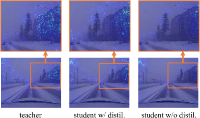
Figure 3: Visualization of the salience maps. With distillation from the teacher, the student is guided to focus on scene-specific objects such as buildings.

5 Conclusion and Limitations

This paper presents DistilVPR, a novel cross-modal distillation pipeline designed for enhancing visual place recognition. We harness multi-agent and multi-manifold relationships to facilitate knowledge exploration, leading to superior performance compared to other distillation baselines.

A limitation of our approach lies in its assumption of identical feature dimensions between teachers and students, potentially restricting its applicability. Nevertheless, this limitation could be addressed by employing a feature adaptor to align the feature dimensions of teachers and students.

6 Acknowledgement

This research is supported by the Singapore Ministry of Education Academic Research Fund Tier 2 grant MOE-T2EP20220-0002, and the National Research Foundation, Singapore and Infocomm Media Development Authority under its Future Communications Research and Development Programme. The computational work for this article was partially performed on resources of the National Supercomputing Centre, Singapore (https://www.nscc.sg).

7 Implementation Details

We choose two SOTA multi-modal place recognition models as teachers, including MinkLoc++ (Komorowski, Wysoczańska, and Trzcinski 2021) and AdaFusion (Lai, Yin, and Scherer 2022). We use their single-modal branches as students to test the effectiveness of cross-modal KD. The scene descriptor dim of the MinkLoc++ series is $384$, while the scene descriptor dim of the AdaFusion series is $256$. We use the Adam optimizer to train both teachers and students. The learning rate is set as $1e-4$ and $1e-3$ for the image branch and the point cloud branch respectively. The learning rate decays by $\times 0.1$ at epoch $40$. Both teacher models and student models are trained for $60$ epochs with $128$ batch size. All experiments are conducted on an A100 GPU using PyTorch. We follow previous works to use the same evaluation protocol, including Average Recall@1 (AR@1) and Average Recall@1% (AR@1%).

8 More Results

8.1 Cross Model Distillation

Although we assume the same output channel sizes for both teacher and student models in the main paper, we have also conducted evaluations in the cross-model scenario, where teacher and student models possess different channel sizes. To mitigate the resultant feature inconsistency, we integrate a fully-connected (fc) layer as an adaptor to harmonize feature channels.

More specifically, we examine two distinct scenarios: one with the adaptor integrated into the teacher model (as shown in Table 7) and the other with the adaptor in the student model (as shown in Table 8). Remarkably, our proposed DistilVPR-SC achieves SOTA performance in 7 out of 8 metrics in the two tables, thereby further validating the efficacy and broad applicability of our approach. Furthermore, when comparing the two methods of implementing the adaptor, it is generally observed that integrating the adaptor within the teacher models yields better results compared to the alternative of placing it within the student models.

Distillation Method	T: MinkLoc++3D		T: AdaFusion-3D
	S: AdaFusion-2D		S: MinkLoc++2D
	AR@1%	AR@1	AR@1%	AR@1
Teacher	98.5	91.0	98.9	91.5
Student w/o distil.	74.5	59.6	75.2	60.0
*KD (Hinton, Vinyals, and Dean 2015)	76.4	58.9	74.7	59.9
AFD (Ji, Heo, and Park 2021)	73.8	56.9	74.2	56.9
EPC-Net (Hui et al. 2022)	75.6	56.9	75.9	58.3
RKD (Park et al. 2019)	76.3	60.1	79.0	62.8
CSD (Wu et al. 2022)	74.7	59.9	76.2	61.2
LSD-Net (Peng et al. 2022)	74.5	58.2	74.7	59.4
MKD (Jin, Wang, and Lin 2023)	76.9	58.8	76.7	60.8
(ours) DistilVPR-S	76.5	60.3	78.1	63.2
(ours) DistilVPR-C	75.8	61.6	77.5	62.1
(ours) DistilVPR-SC	77.6	63.1	80.7	66.3

Table 7: Cross model 3D-to-2D distillation comparison on the Boreas dataset. The adaptor is equipped on the teacher model.

Distillation Method	T: MinkLoc++3D		T: AdaFusion-3D
	S: AdaFusion-2D		S: MinkLoc++2D
	AR@1%	AR@1	AR@1%	AR@1
Teacher	98.5	91.0	98.9	91.5
Student w/o distil.	74.5	59.6	75.2	60.0
*KD (Hinton, Vinyals, and Dean 2015)	74.2	58.6	77.1	61.1
AFD (Ji, Heo, and Park 2021)	76.1	59.6	75.7	58.8
EPC-Net (Hui et al. 2022)	75.4	60.5	75.4	60.6
RKD (Park et al. 2019)	75.9	62.0	75.1	60.4
CSD (Wu et al. 2022)	74.1	60.2	76.2	60.9
LSD-Net (Peng et al. 2022)	71.6	58.5	74.9	59.2
MKD (Jin, Wang, and Lin 2023)	73.4	58.7	76.0	61.2
(ours) DistilVPR-S	76.6	61.6	74.7	61.7
(ours) DistilVPR-C	76.6	61.7	75.8	60.6
(ours) DistilVPR-SC	77.4	62.4	76.1	63.4

Table 8: Cross model 3D-to-2D distillation comparison on the Boreas dataset. The adaptor is equipped on the student model.

8.2 Visualization

We present visualizations of several place recognition examples in Fig. 4. These examples showcase the effectiveness of the distillation approaches in enhancing performance. Notably, in comparison to the results obtained using RKD (Park et al. 2019), our proposed DistilVPR-SC yields better outcomes, particularly evident in the accurate recognition of challenging rain scenes.

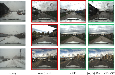
Figure 4: Visualizations of place recognition examples.

9 Compared Baselines

The baselines we used in our experiments can be classified into direct KD solutions and relational KD solutions.

• Direct KD baselines include: vanilla KD (Hinton, Vinyals, and Dean 2015), AFD (Ji, Heo, and Park 2021), EPC-Net (Hui et al. 2022).

• Relational KD baselines include: RKD (Park et al. 2019), CSD (Wu et al. 2022), LSD-Net (Peng et al. 2022), MKD (Jin, Wang, and Lin 2023).

10 Open Sources

The two used datasets are both open-source datasets and can be available online.

• The Oxford RobotCar dataset.
  https://robotcar-dataset.robots.ox.ac.uk/

• The Boreas dataset.
  https://www.boreas.utias.utoronto.ca/#/

Our code is mainly built based on the following repositories.

• MinkLoc++
  https://github.com/jac99/MinkLocMultimodal

• AdaFusion
  https://github.com/MetaSLAM/AdaFusion

References

- Arandjelovic et al. (2016) Arandjelovic, R.; Gronat, P.; Torii, A.; Pajdla, T.; and Sivic, J. 2016. NetVLAD: CNN architecture for weakly supervised place recognition. In Proceedings of the IEEE conference on computer vision and pattern recognition, 5297–5307.
- Burnett et al. (2022) Burnett, K.; Yoon, D. J.; Wu, Y.; Li, A. Z.; Zhang, H.; Lu, S.; Qian, J.; Tseng, W.-K.; Lambert, A.; Leung, K. Y.; et al. 2022. Boreas: A multi-season autonomous driving dataset. arXiv preprint arXiv:2203.10168.
- Chen et al. (2023) Chen, C.; Liu, X.; Li, Y.; Ding, L.; and Feng, C. 2023. DeepMapping2: Self-Supervised Large-Scale LiDAR Map Optimization. In Proceedings of the IEEE/CVF Conference on Computer Vision and Pattern Recognition, 9306–9316.
- Engel, Koltun, and Cremers (2017) Engel, J.; Koltun, V.; and Cremers, D. 2017. Direct sparse odometry. IEEE transactions on pattern analysis and machine intelligence, 40(3): 611–625.
- Gálvez-López and Tardos (2012) Gálvez-López, D.; and Tardos, J. D. 2012. Bags of binary words for fast place recognition in image sequences. IEEE Transactions on Robotics, 28(5): 1188–1197.
- Hinton, Vinyals, and Dean (2015) Hinton, G.; Vinyals, O.; and Dean, J. 2015. Distilling the knowledge in a neural network. arXiv preprint arXiv:1503.02531.
- Hou et al. (2022) Hou, Y.; Zhu, X.; Ma, Y.; Loy, C. C.; and Li, Y. 2022. Point-to-voxel knowledge distillation for lidar semantic segmentation. In Proceedings of the IEEE/CVF conference on computer vision and pattern recognition, 8479–8488.
- Hui et al. (2022) Hui, L.; Cheng, M.; Xie, J.; Yang, J.; and Cheng, M.-M. 2022. Efficient 3D point cloud feature learning for large-scale place recognition. IEEE Transactions on Image Processing, 31: 1258–1270.
- Jégou et al. (2011) Jégou, H.; Perronnin, F.; Douze, M.; Sánchez, J.; Pérez, P.; and Schmid, C. 2011. Aggregating local image descriptors into compact codes. IEEE transactions on pattern analysis and machine intelligence, 34(9): 1704–1716.
- Ji, Heo, and Park (2021) Ji, M.; Heo, B.; and Park, S. 2021. Show, attend and distill: Knowledge distillation via attention-based feature matching. In Proceedings of the AAAI Conference on Artificial Intelligence, 7945–7952.
- Jin, Wang, and Lin (2023) Jin, Y.; Wang, J.; and Lin, D. 2023. Multi-Level Logit Distillation. In Proceedings of the IEEE/CVF Conference on Computer Vision and Pattern Recognition, 24276–24285.
- Komorowski (2021) Komorowski, J. 2021. MinkLoc3d: Point cloud based large-scale place recognition. In Proceedings of the IEEE/CVF Winter Conference on Applications of Computer Vision, 1790–1799.
- Komorowski, Wysoczańska, and Trzcinski (2021) Komorowski, J.; Wysoczańska, M.; and Trzcinski, T. 2021. MinkLoc++: Lidar and monocular image fusion for place recognition. In 2021 International Joint Conference on Neural Networks (IJCNN), 1–8. IEEE.
- Lai, Yin, and Scherer (2022) Lai, H.; Yin, P.; and Scherer, S. 2022. AdaFusion: Visual-lidar fusion with adaptive weights for place recognition. IEEE Robotics and Automation Letters, 7(4): 12038–12045.
- Liu, Nickel, and Kiela (2019) Liu, Q.; Nickel, M.; and Kiela, D. 2019. Hyperbolic graph neural networks. Advances in neural information processing systems, 32.
- Lu et al. (2020) Lu, Y.; Yang, F.; Chen, F.; and Xie, D. 2020. PIC-Net: Point cloud and image collaboration network for large-scale place recognition. arXiv preprint arXiv:2008.00658.
- Maddern et al. (2017) Maddern, W.; Pascoe, G.; Linegar, C.; and Newman, P. 2017. 1 year, 1000 km: The Oxford RobotCar dataset. The International Journal of Robotics Research, 36(1): 3–15.
- Oertel, Cieslewski, and Scaramuzza (2020) Oertel, A.; Cieslewski, T.; and Scaramuzza, D. 2020. Augmenting visual place recognition with structural cues. IEEE Robotics and Automation Letters, 5(4): 5534–5541.
- Pan et al. (2021) Pan, Y.; Xu, X.; Li, W.; Cui, Y.; Wang, Y.; and Xiong, R. 2021. CORAL: Colored structural representation for bi-modal place recognition. In 2021 IEEE/RSJ International Conference on Intelligent Robots and Systems (IROS), 2084–2091. IEEE.
- Park et al. (2019) Park, W.; Kim, D.; Lu, Y.; and Cho, M. 2019. Relational knowledge distillation. In Proceedings of the IEEE/CVF conference on computer vision and pattern recognition, 3967–3976.
- Peng et al. (2022) Peng, G.; Huang, Y.; Li, H.; Wu, Z.; and Wang, D. 2022. LSDNet: A Lightweight Self-Attentional Distillation Network for Visual Place Recognition. In 2022 IEEE/RSJ International Conference on Intelligent Robots and Systems (IROS), 6608–6613. IEEE.
- Qi et al. (2017) Qi, C. R.; Su, H.; Mo, K.; and Guibas, L. J. 2017. Pointnet: Deep learning on point sets for 3d classification and segmentation. In Proceedings of the IEEE conference on computer vision and pattern recognition, 652–660.
- Sarlin et al. (2019) Sarlin, P.-E.; Cadena, C.; Siegwart, R.; and Dymczyk, M. 2019. From coarse to fine: Robust hierarchical localization at large scale. In Proceedings of the IEEE/CVF Conference on Computer Vision and Pattern Recognition, 12716–12725.
- Sarlin et al. (2022) Sarlin, P.-E.; Dusmanu, M.; Schönberger, J. L.; Speciale, P.; Gruber, L.; Larsson, V.; Miksik, O.; and Pollefeys, M. 2022. LaMAR: Benchmarking localization and mapping for augmented reality. In Computer Vision–ECCV 2022: 17th European Conference, Tel Aviv, Israel, October 23–27, 2022, Proceedings, Part VII, 686–704. Springer.
- She et al. (2023) She, R.; Kang, Q.; Wang, S.; Yáng, Y.-R.; Zhao, K.; Song, Y.; and Tay, W. P. 2023. Robustmat: Neural diffusion for street landmark patch matching under challenging environments. IEEE Transactions on Image Processing.
- Shi et al. (2023) Shi, J.; Chen, G.; Zhao, Y.; and Tao, R. 2023. Synchrosqueezed Fractional Wavelet Transform: A New High-Resolution Time-Frequency Representation. IEEE Transactions on Signal Processing, 71: 264–278.
- Tifrea, Bécigneul, and Ganea (2018) Tifrea, A.; Bécigneul, G.; and Ganea, O.-E. 2018. Poincar’e glove: Hyperbolic word embeddings. arXiv preprint arXiv:1810.06546.
- Uy and Lee (2018) Uy, M. A.; and Lee, G. H. 2018. PointNetVLAD: Deep point cloud based retrieval for large-scale place recognition. In Proceedings of the IEEE conference on computer vision and pattern recognition, 4470–4479.
- Wang et al. (2023a) Wang, S.; Kang, Q.; She, R.; Wang, W.; Zhao, K.; Song, Y.; and Tay, W. P. 2023a. HypLiLoc: Towards effective liDAR pose regression with hyperbolic fusion. In Proceedings of the IEEE/CVF Winter Conference on Applications of Computer Vision.
- Wang et al. (2023b) Wang, S.; Li, W.; Liu, W.; Liu, X.; and Zhu, J. 2023b. LiDAR2Map: In Defense of LiDAR-Based Semantic Map Construction Using Online Camera Distillation. In Proceedings of the IEEE/CVF Conference on Computer Vision and Pattern Recognition, 5186–5195.
- Wu et al. (2022) Wu, H.; Wang, M.; Zhou, W.; Li, H.; and Tian, Q. 2022. Contextual similarity distillation for asymmetric image retrieval. In Proceedings of the IEEE/CVF Conference on Computer Vision and Pattern Recognition, 9489–9498.
- Yan et al. (2022) Yan, X.; Gao, J.; Zheng, C.; Zheng, C.; Zhang, R.; Cui, S.; and Li, Z. 2022. 2dpass: 2d priors assisted semantic segmentation on lidar point clouds. In Computer Vision–ECCV 2022: 17th European Conference, Tel Aviv, Israel, October 23–27, 2022, Proceedings, Part XXVIII, 677–695. Springer Nature Switzerland Cham.
- Zhao et al. (2023) Zhao, K.; Kang, Q.; Song, Y.; She, R.; Wang, S.; and Tay, W. P. 2023. Adversarial robustness in graph neural networks: A Hamiltonian approach. arXiv preprint arXiv:2310.06396.
- Zhou et al. (2023) Zhou, S.; Liu, W.; Hu, C.; Zhou, S.; and Ma, C. 2023. UniDistill: A Universal Cross-Modality Knowledge Distillation Framework for 3D Object Detection in Bird’s-Eye View. In Proceedings of the IEEE/CVF Conference on Computer Vision and Pattern Recognition, 5116–5125.