A Symmetric Multigrid-Preconditioned Krylov Subspace Solver for Stokes Equation

Abstract

Numerical solution of discrete PDEs corresponding to saddle point problems is highly relevant to physical systems such as Stokes flow. However, scaling up numerical solvers for such systems is often met with challenges in efficiency and convergence. Multigrid is an approach with excellent applicability to elliptic problems such as the Stokes equations, and can be a solution to such challenges of scalability and efficiency. The degree of success of such methods, however, is highly contingent on the design of key components of a multigrid scheme, including the hierarchy of discretizations, and the relaxation scheme used. Additionally, in many practical cases, it may be more effective to use a multigrid scheme as a preconditioner to an iterative Krylov subspace solver, as opposed to striving for maximum efficacy of the relaxation scheme in all foreseeable settings. In this paper, we propose an efficient symmetric multigrid preconditioner for the Stokes Equations on a staggered finite-difference discretization. Our contribution is focused on crafting a preconditioner that (a) is symmetric indefinite, matching the property of the Stokes system itself, (b) is appropriate for preconditioning the SQMR iterative scheme [1], and (c) has the requisite symmetry properties to be used in this context. In addition, our design is efficient in terms of computational cost and facilitates scaling to large domains.

[inst1]organization=The computer sciences department, University of Wisconsin-Madison,addressline=1210 W Dayton St, city=Madison, postcode=53706, state=Wisconsin, country=United States

We propose a multigrid-preconditioned SQMR method for symmetric saddle-point problems within the context of the Stokes equations.

We design effective symmetric smoother for both the distributive smoother and Vanka smoother, combining them to achieve a balance between convergence rates and computational time per iteration.

We compare the performance of our new multigrid-preconditioned solver with the classical multigrid method on both 2D and 3D benchmarks.

1 Introduction

Saddle-point problems arise in many fields such as fluid dynamics [2, 3], structure mechanics [4, 5] and magnetohydrodynamics [6]. As modern computational devices develop, a requirement for solving large-scale problems arises. Multigrid methods [7] are well-known for their potential scalability in handling large-scale problems with the advantage of linear time and space complexity. Although the convergence rates of multigrid methods are independent of problem sizes, the design and optimization of multigrid components, such as relaxation schemes, can significantly impact convergence rates. The relaxation scheme, often referred to as a smoother in multigrid, comprises various classical techniques, including the distributive smoother [8], Uzawa smoother [9], Braess-Sarazin smoother [10] and Vanka smoother [11]. The distributive smoother transforms the original system equations into a right-preconditioned system, aiming to improve properties like condition numbers. It has been studied for solving problems like the Stokes equations [8, 12, 13] and the Oseen equations [14]. The Uzawa smoother transforms indefinite systems into positive definite ones by using Schur complement, with applications in solving the Stokes equations [15] and poroelasticity equations [16]. The Braess-Sarazin smoother is a variant of the pressure correction steps in SIMPLE-type algorithms [17]. It also relies on the approximation of Schur complement and has been introduced for tackling challenges such as the Stokes equations [10, 18] and magnetohydrodynamic equations [19]. In contrast to the previous three smoothers, the Vanka smoother focuses on solving local overlapping saddle-point problems instead of the entire saddle-point system. While the Vanka smoother shows high efficiency in each iteration, it comes with higher per-iteration costs compared to other smoothing methods. It has proven effective in the Stokes equations [11, 20] and poroelasticity equations [21]. In addition to the choice of smoother, the convergence of multigrid also depends on factors like grid-operators [22], discretization methods [23], and even on some problem-specific parameters [24].

Considering the sensitivity of multigrid methods, they can be more effective when used as a preconditioner to an iterative Krylovs subspace solver. The multigrid-preconditioned conjugate gradient (MGPCG) method [25] is the prototypical approach for solving positive definite systems such as Poisson’s equation. However, for saddle-point problems, a more general Krylov subspace solver is required. The generalized minimal residual (GMRes) method [26] emerges as the most common choice in this context, promising convergence for any asymmetric indefinite system. The multigrid-preconditioned GMRes has been employed in addressing transport equations [27], advection-diffusion equations [28, 29] and Navier-Stokes equations [30]. Despite of the indefiniteness of saddle-point problems, symmetry prevails in many situations such as the Stokes equation, Oseen equations and Helmholtz equation. The minimal residual (Minres) [31] method, designed for symmetric indefinite systems, consumes both less memory and less computational time than GMRes in one iteration while maintaining similar convergence rates. It appears to be a more promising option in these symmetric scenarios. However, Minres has the limitation in that it can only be paired with positive definite preconditioners, making it incompatible with multigrid preconditioning. For this reason, we investigate the symmetric quasi-minimal residual (SQMR) method [1], a variant of MINRES with identical work and storage requirements. SQMR supports symmetric indefinite preconditioners, opening up opportunities for the use of multigrid as the preconditioner. To the best of our knowledge, no multigrid-preconditioned SQMR has been developed for symmetric saddle-point problems.

Since SQMR requires symmetric indefinite preconditioners, the smoothing step of multigrid must also be symmetric. Inspired by the symmetric Gauss-Seidel method, we design an effective symmetric distributive smoother and Vanka smoother in this work. The main idea behind the symmetric smoother involves relaxation in some specific order, followed by relaxation in the exact reverse order. Our primary focus is on the multigrid-preconditioned SQMR method, utilizing a staggered finite-difference discretization of the Stokes equations as the model problem. The main contributions of this work can be summarized as follows:

• We propose a multigrid-preconditioned SQMR method for symmetric saddle-point problems within the context of the Stokes equations.

• We design effective symmetric smoother for both the distributive smoother and Vanka smoother, combining them to achieve a balance between convergence rates and computational time per iteration.

• We compare the performance of our new multigrid-preconditioned solver with the classical multigrid method on both 2D and 3D benchmarks.

The remaining structure of the paper is as follows: In section 2, we introduce the finite-difference discretization of the Stokes equation and explain how we apply multigrid. In section 3, we discuss how we ensure the symmetry of the distributive smoother and Vanka smoother. In section 4, we propose our approach to use multigrid as a preconditioner for SQMR. In section 5, we describe our discrete domain design used for boundary conditions. In section 6, we compare the performance of our multigrid-preconditioned solver with the classical multigrid method on both 2D and 3D benchmarks. Finally, we draw our conclusions in section 7.

2 Multigrid for the Stokes equation

In this work, we consider the following Stokes equations, which apply to both 2D and 3D scenarios:

$$\begin{split}-\eta\Delta\mathbf{u}+\nabla p=\mathbf{f}\\ -\nabla\cdot\mathbf{u}=\mathbf{0}\end{split}$$ (1)

where $\mathbf{u}=(u,v)^{T}$ (2D) or $\mathbf{u}=(u,v,w)^{T}$ (3D) is the fluid velocity vector field, $p$ is the pressure scalar field, $\mathbf{f}$ is the body force vector field and $\eta$ is the fluid viscosity, together with a suitable boundary condition.

For the discretization of the Stokes equations, we employ the standard staggered finite-difference method known as the marker-and-cell (MAC) scheme [7]. As shown in Fig. 1, the velocity components are located at the center of each edge in 2D or each surface in 3D, while the pressure variables are located at the center of each square in 2D or each cube in 3D. Although this discretization can be extended to non-uniform grid sizes $h_{x}\neq h_{y}\neq h_{z}$, we focus on uniform meshes with a grid size of $h=h_{x}=h_{y}=h_{z}$. The discretization employs central differences for the operators in the Stokes equations. Specifically, the Laplacian $\Delta$ operator is discretized using a five-point stencil in 2D and a seven-point stencil in 3D, while $\nabla$ operator is discretized via central difference approximation for velocity components. $\nabla\cdot$ operator is discretized using central differences for pressure. This leads to the linear system discretized from the Stokes equations 1:

$$\mathbf{L}\mathbf{x}=\begin{pmatrix}\mathbf{A}&\mathbf{B}^{T}\\ \mathbf{B}&\mathbf{0}\\ \end{pmatrix}\begin{pmatrix}\mathbf{u}\\ p\\ \end{pmatrix}=\begin{pmatrix}\mathbf{f}\\ 0\\ \end{pmatrix}=\mathbf{b}$$ (2)

where $\mathbf{A}$, $\mathbf{B}$ and $\mathbf{B}^{T}$ represent discrete approximations of operators $-\eta\Delta$, $-\nabla\cdot$ and $\nabla$ operators respectively.

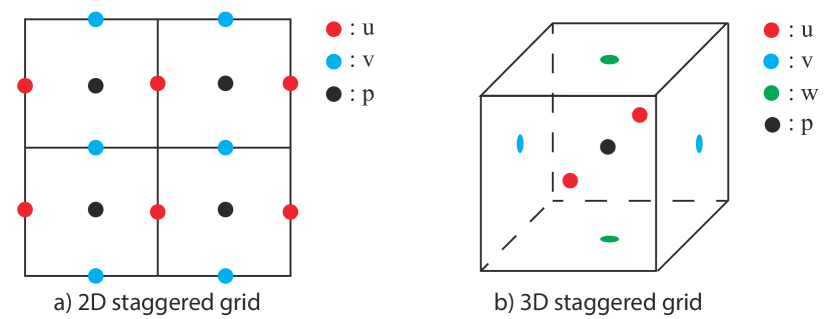
Figure 1: The staggered grid discretization in 2D (left) and 3D (right)

Then we discuss the skeleton of our multigrid method. When it comes to balancing computational time and convergence rates, we have various multigrid methods to choose from, such as V-cycle, W-cycle and F-cycle [32]. For efficiency, we opt for V-cycle, which runs faster per iteration but converges slightly slower than the others. Since multigrid is intended to be used as a preconditioner, V-cycle is an adequate design. The recursive V-cycle procedure is outlined in Alg. 1, where the superscript $h$ denotes discretization at grid size $h$. It is worth mentioning that we rediscretize $\mathbf{L}^{2h}$ at a coarser level rather than using Galerkin coarsening [23], using finite-difference discretization. The locations of $u$ and $p$ components of 2D fine grid and coarse grid are shown in Fig. 2. It can be analogized to $v$ component and 3D cases.

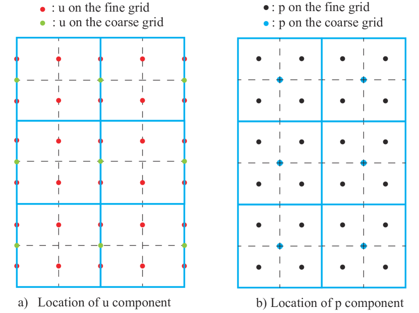
Figure 2: 2D discretization on fine and coarse level

As we mentioned above, the restriction operator $\mathbf{R}$ and prolongation operator $\mathbf{P}$ can also influence convergence rates for the Stokes equations. Some common combinations have been investigated by Niestegge [22]. To maintain the symmetry (discussed further later), we must use the transposed operators for $\mathbf{R}$ and $\mathbf{P}$, meaning $\mathbf{P}=c\mathbf{R}^{T}$ with $c$ is typically 4 for 2D and 8 for 3D. To balance the symmetry and the convergence rates, we use the bilinear interpolation for velocities and constant per-cell interpolation for pressures as the prolongation operator. The restriction operator is exactly transposed of the prolongation operator divided by $c$. Fig. 3 illustrates how we prolongate on $u$ component and $p$ component in 2D cases.

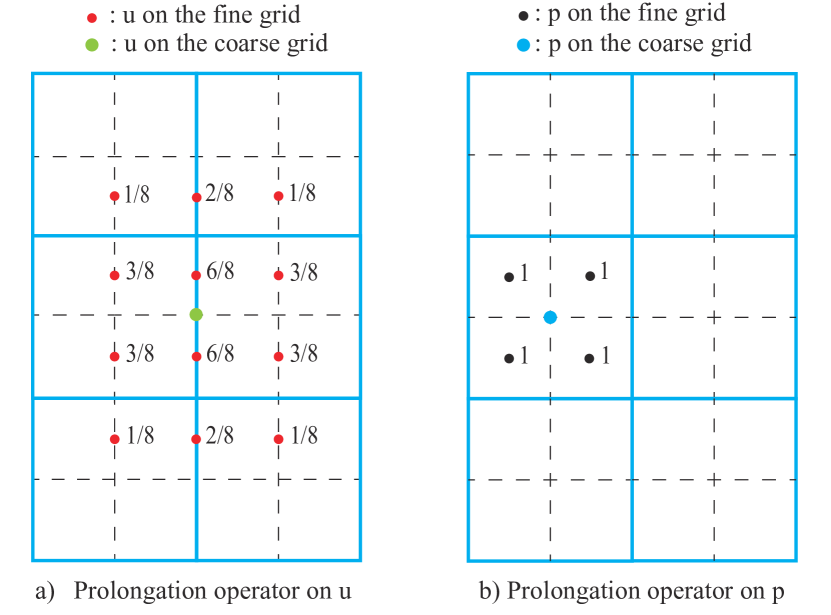
Figure 3: 2D Prolongation Operator

1:Input: System matrix $\mathbf{L}^{h}$, right hand side $\mathbf{b}^{h}$, initial guess $\mathbf{x}^{h}_{0}$ with grid size $h$ and multigrid level $n\geq 1$

2:Output: Solution $\mathbf{x}^{h}$

3:procedure V-cycle($\mathbf{L}^{h}$, $\mathbf{b}^{h}$, $\mathbf{x}^{h}_{0}$, $n$)

4:     if $n=1$ then

5:         Solve $\mathbf{L}^{h}\mathbf{x}^{h}=\mathbf{b}^{h}$ exactly

6:     else

7:         $\mathbf{x}^{h}\leftarrow\text{Smoothing}(\mathbf{L}^{h},\mathbf{x}^{h}_{0},\mathbf{b}^{h})$

8:         $\mathbf{r}^{h}\leftarrow\mathbf{b}^{h}-\mathbf{L}^{h}\mathbf{x}^{h}$

9:         $\mathbf{r}^{2h}\leftarrow\mathbf{R}^{h}\mathbf{r}^{h}$ $\triangleright$ $\mathbf{R}^{h}$ is the restriction operator

10:         $\mathbf{L}^{2h}\leftarrow\text{Rediscretized from coarser level}$

11:         $\mathbf{e}^{2h}\leftarrow\text{Recursively call }\text{V-cycle}(\mathbf{L}^{2h},\mathbf{r}^{2h},\mathbf{0}^{2h},n-1)$ 

12:         $\mathbf{e}^{h}\leftarrow\mathbf{P}^{h}\mathbf{e}^{2h}$; $\triangleright$ $\mathbf{P}^{h}$ is the prolongation operator

13:         $\mathbf{x}^{h}\leftarrow\mathbf{x}^{h}+\mathbf{e}^{h}$

14:         $\mathbf{x}^{h}\leftarrow\text{Smoothing}(\mathbf{L}^{h},\mathbf{x}^{h},\mathbf{b}^{h})$ 

15:     end if

16:end procedure

Algorithm 1 Recursive V-cycle

3 Smoothing step and symmetry

As discussed in MGPCG [25], the symmetry of the V-cycle can be reduced to the symmetry of the smoothing step. A smoothing step can be formulated as

$$\mathbf{x}^{k+1}=\mathbf{x}^{k}+\mathbf{S}(\mathbf{b}-\mathbf{L}\mathbf{x}^{k})$$ (3)

where $k$ denotes the iteration step and $\mathbf{S}$ is the smoother operator. For example, classical Gauss-Seidel smoothing can be expressed as $\mathbf{S}_{GS}=\mathbf{G}^{-1}$ with $\mathbf{G}$ being the lower triangular component of system matrix $\mathbf{L}$. Similarly, the weighted Jacobi method can be written as $\mathbf{S}_{WJ}=\omega\mathbf{D}$, where $\omega$ is the damping factor and $\mathbf{D}$ is the diagonal component of $\mathbf{L}$. We can observe that $\mathbf{x}^{k}$ must be a linear transformation of $\mathbf{b}$ when $\mathbf{x}^{0}=\mathbf{0}$, implying $\mathbf{x}^{k}=\mathbf{C}\mathbf{b}$. The smoothing step is symmetric to design a multigrid preconditioner if and only if $\mathbf{C}$ is symmetric. This simplification occurs when we employ the same smoother before and after the rediscretization step, and use the transposed operator for $\mathbf{R}$ and $\mathbf{P}$. In this section, we discuss the design of symmetric operators for both the distributive smoother and Vanka smoother. We also explore how these operators can be combined while maintaining symmetry.

3.1 Symmetric distributive smoother

The idea of the distributive smoother can be viewed as a transformation of the original system $\mathbf{L}\mathbf{x}=\mathbf{b}$ into a right-preconditioned system $\mathbf{L}\mathbf{M}\mathbf{y}=\mathbf{b}$, where $\mathbf{M}\mathbf{y}=\mathbf{x}$. For the Stokes equations, the transformed system can be formulated as

$$\mathbf{L}\mathbf{M}\mathbf{y}=\begin{pmatrix}\mathbf{A}&\mathbf{B}^{T}\\ \mathbf{B}&\mathbf{0}\\ \end{pmatrix}\begin{pmatrix}\mathbf{I}&-\mathbf{B}^{T}\\ \mathbf{0}&\eta\mathbf{B}\mathbf{B}^{T}\\ \end{pmatrix}\begin{pmatrix}\tilde{\mathbf{u}}\\ \tilde{p}\\ \end{pmatrix}=\mathbf{b}$$ (4)

which yields

$$\begin{split}\mathbf{L}\mathbf{M}&=\begin{pmatrix}\mathbf{A}&\mathbf{B}^{T}\\ \mathbf{B}&\mathbf{0}\\ \end{pmatrix}\begin{pmatrix}\mathbf{I}&-\mathbf{B}^{T}\\ \mathbf{0}&\eta\mathbf{B}\mathbf{B}^{T}\\ \end{pmatrix}=\begin{pmatrix}-\eta\Delta^{h}&\nabla^{h}\\ -\nabla\cdot^{h}&\mathbf{0}\\ \end{pmatrix}\begin{pmatrix}\mathbf{I}&-\nabla^{h}\\ \mathbf{0}&-\eta\nabla\cdot^{h}\nabla^{h}\\ \end{pmatrix}\\ &=\begin{pmatrix}-\eta\Delta^{h}&\eta\Delta^{h}\nabla^{h}-\eta\nabla^{h}(\nabla\cdot^{h}\nabla^{h})\\ -\nabla\cdot^{h}&\nabla\cdot^{h}\nabla^{h}\\ \end{pmatrix}=\begin{pmatrix}-\eta\Delta^{h}&\mathbf{0}\\ -\nabla\cdot^{h}&\nabla\cdot^{h}\nabla^{h}\\ \end{pmatrix}\\ \end{split}$$ (5)

The top right block is $\mathbf{0}$ due to the commutativity of $\Delta$ and $\nabla$ operators, which is a property that Stokes equation specifically holds under a finite difference discretization. It’s important to note that when alternative discretization methods like finite element are employed, the top-right block may not be exact zero but only asymptotically zero up to truncation error. Furthermore, we should also notice that the matrix can be converted into discrete operators only when the degrees of freedom are in the interior region, free from the constraints of the boundary conditions. The introduction of the distributive matrix $\mathbf{M}$ is motivated by the fact that $\mathbf{L}\mathbf{M}$ forms a block upper triangular matrix with the Laplacian operator on the diagonal block. This structure allows us to apply classical smoothing methods like Gauss-Seidel or weighted Jacobi on $\mathbf{L}\mathbf{M}$ matrix, leveraging their effectiveness on the Laplacian operator. From that, $\delta\mathbf{y}$ is obtained to compute corrections $\delta\mathbf{x}=\mathbf{M}\delta\mathbf{y}$. The smoothing operator of distributive Gauss-Seidel (DGS) and distributive weighted Jacobi (DWJ) can be represented as $\mathbf{S}_{DGS}=\mathbf{M}\mathbf{\tilde{G}}^{-1}$ and $\mathbf{S}_{DWJ}=\omega\mathbf{M}\mathbf{\tilde{D}}^{-1}$ where $\mathbf{\tilde{G}}$ and $\mathbf{\tilde{D}}$ is the upper triangular and diagonal component of system matrix $\mathbf{L}\mathbf{M}$. Instead of computing the entire $\mathbf{L}\mathbf{M}$ matrix and applying Gauss-Seidel or weighted Jacobi, this process can be simplified by storing the diagonal part of $\mathbf{L}\mathbf{M}$ and using the connection $\mathbf{x}=\mathbf{M}\mathbf{y}$. Alg. 2 provides a detailed example of the simplification of DGS smoothing. A similar approach can be employed for DWJ smoothing.

1:Input: System matrix $\mathbf{L}$, initial guess $\mathbf{x}_{0}$ and right hand side $\mathbf{b}$

2:Output: Solution $\mathbf{x}$

3:procedure DGS($\mathbf{L}$, $\mathbf{x}_{0}$, $\mathbf{b}$)

4:     Compute distributive matrix $\mathbf{M}$

5:     $\mathbf{d}=\mathbf{0}$

6:     for $j=1,2,...$ do

7:         $\mathbf{d}_{j}\leftarrow\mathbf{L}_{j,}\cdot\mathbf{M}_{,j}$

8:         $\triangleright$ where $\mathbf{L}_{j,}$ is the $j$th row of $\mathbf{L}$ and $\mathbf{M}_{,j}$ is the $j$th column of $\mathbf{M}$

9:     end for

10:     $\mathbf{x}^{h}\leftarrow\mathbf{x}_{0}^{h}$

11:     for $j=1,2,...$ do

12:         $r\leftarrow\mathbf{b}_{j}-\mathbf{L}_{j,}\mathbf{x}$

13:         $\mathbf{x}\leftarrow\mathbf{x}+\frac{r}{\mathbf{d}_{j}}\mathbf{M}_{,j}$

14:     end for

15:end procedure

Algorithm 2 Distributive Gauss-Seidel Smoothing

As we mentioned above, we aim to design a symmetric smoother. However, the symmetry of distributive smoothing is hindered by right-preconditioning. To maintain symmetry, we introduce left-preconditioning of the distributive smoother as follows

$$\mathbf{M}^{T}\mathbf{L}\mathbf{x}=\begin{pmatrix}\mathbf{I}&\mathbf{0}\\ -\mathbf{B}&\eta\mathbf{B}\mathbf{B}^{T}\\ \end{pmatrix}\begin{pmatrix}\mathbf{A}&\mathbf{B}^{T}\\ \mathbf{B}&\mathbf{0}\\ \end{pmatrix}\begin{pmatrix}\mathbf{u}\\ p\\ \end{pmatrix}=\mathbf{M}^{T}\mathbf{b}$$ (6)

It’s obvious that $\mathbf{M}^{T}\mathbf{L}=(\mathbf{LM})^{T}$ due to the symmetry of $\mathbf{L}$. By combining right DWJ with left DWJ or right DGS in a specific order with left DGS in the exact reverse order, the smoother can recover its symmetry. A proof for symmetric DGS can be found in A, and a similar proof applies to DWJ. Despite the efficiency of the distributive smoother, its convergence heavily relies on the commutativity of $\Delta$ and $\nabla$ operators in the interior region. This property doesn’t hold near the boundary, potentially leading to divergence. Therefore, it’s essential to employ more robust smoother near the boundary.

3.2 Symmetric Vanka smoother

The Vanka smoother is more powerful but with a higher computational cost per iteration compared to the distributive smoother. It can be viewed as a specific type of Schwarz smoother [33]. The fundamental idea behind the Vanka smoother is to solve the Stokes equations locally, subdomain by subdomain, wherein all degrees of freedom within one subdomain are updated simultaneously. Similar to the other smoother, the Vanka smoother can be expressed in the format of Eq. 3. In the Vanka smoother, we divide the entire problem domain $D$ into $n$ potentially overlapping subdomains $\{D_{1},...,D_{n}\}$ as shown in Fig. 4. Each subdomain can be viewed as a local saddle-point problem. When solving each subdomain problem sequentially, akin to Gauss-Seidel, it’s called the multiplicative Vanka smoother. The smoother operator can be defined as

$$\mathbf{S}_{MV}=[\mathbf{I}-\prod_{i=1}^{n}(\mathbf{I}-\mathbf{C}_{i}^{T}(\mathbf{C}_{i}\mathbf{L}\mathbf{C}_{i}^{T})^{-1}\mathbf{C}_{i}\mathbf{L})]\mathbf{L}^{-1}$$ (7)

where $\mathbf{C}_{i}$ represents the selection matrix from domain $D$ to domain $D_{i}$. Alternatively, if each subdomain problem is solved simultaneously as Jacobi method, it’s the addictive Vanka smoother. The smoother operator for this approach is defined as

$$\mathbf{S}_{AV}=\sum_{i=1}^{n}\mathbf{C}_{i}^{T}(\mathbf{C}_{i}\mathbf{L}\mathbf{C}_{i}^{T})^{-1}\mathbf{C}_{i}$$ (8)

We prove that the addictive Vanka smoother is always symmetric in B. To ensure the symmetry in the multiplicative Vanka smoother, we adopt a similar approach to symmetric Gauss-Seidel. We solve each subdomain from domain $D_{1}$ to $D_{n}$, and then in reverse order from $D_{n}$ to $D_{1}$ again. The symmetry for our symmetric multiplicative Vanka smoother is shown in C.

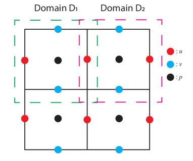
Figure 4: Vanka Smoother on 2D example

3.3 Symmetric integration of smoother

As previously discussed, these two smoother provide advantages depending on the region of the computational domain. Symmetric distributive smoother demonstrates reliability when applied to the interior region, while symmetric Vanka smoother exhibits greater suitability near the boundary. However, despite each can be made symmetric on its own, it’s not universally true that any combination will inherently retain symmetry. To ensure strict symmetry with the multigrid framework, we propose the following smoothing step algorithm. First, we partition the unknowns into two non-overlapping sets: boundary set $V_{1}$ and interior set $V_{2}$. Then we apply symmetric Vanka smoother to $V_{1}$, symmetric distributive smoother to $V_{2}$ and another symmetric Vanka smoother to $V_{1}$ again. The detailed algorithm is shown in Alg. 3, with a formal proof for its symmetry provided in D. Practically, DGS smoother is used instead of DWJ smoother because it has a faster convergence rate but a similar time cost.

This approach leverages the strengths of both smoothers. On one hand, the larger size of $V_{2}$ ensures that symmetric Vanka smoother isn’t overused, enhancing computational efficiency. On the other hand, employing symmetric Vanka smoother near the boundary helps prevent the potential divergence issues of symmetric distributive smoother. Therefore, this integration approach is a superior choice in practical applications compared to using either smoother alone.

1:Input: System matrix $\mathbf{L}^{h}$, initial guess $\mathbf{x}^{h}_{0}$ and right hand side $\mathbf{b}^{h}$

2:Output: Solution $\mathbf{x}^{h}$

3:procedure Smoothing($\mathbf{L}^{h}$, $\mathbf{x}^{h}_{0}$, $\mathbf{b}^{h}$)

4:     Partition $\mathbf{x}^{h}$ into two non-overlapping sets: boundary set $V_{1}$ and interior set $V_{2}$

5:     $\mathbf{x}^{h}\leftarrow\text{Symmetric\_Vanka}(\mathbf{L}^{h},\mathbf{x}^{h}_{0},\mathbf{b}^{h})$ on the boundary set $V_{1}$

6:     $\mathbf{x}^{h}\leftarrow\text{Symmetric\_Distributive}(\mathbf{L}^{h},\mathbf{x}^{h}_{0},\mathbf{b}^{h})$ on the interior set $V_{2}$

7:     $\mathbf{x}^{h}\leftarrow\text{Symmetric\_Vanka}(\mathbf{L}^{h},\mathbf{x}^{h}_{0},\mathbf{b}^{h})$ on the boundary set $V_{1}$

8:end procedure

Algorithm 3 Smoothing

4 Preconditioning

Although the use of Vanka smoother significantly improves convergence near the boundary, multigrid is more stable to be used as the preconditioner for the Krylov subspace solver. SQMR is known for its lower computational time and storage requirements, and supports arbitrary symmetric preconditioners, including indefinite ones from multigrid V-cycle. Therefore, we propose using our multigrid as the preconditioner for SQMR. The multigrid preconditioner is outlined in Alg. 4. It’s worth mentioning that not any multigrid V-cycle can be used as the preconditioner. This procedure must be equivalent to $\mathbf{t}\leftarrow\mathbf{M}^{-1}\mathbf{s}_{0}$ with some symmetric matrix $\mathbf{M}$. Fortunately, as we prove in the appendix, our multigrid indeed satisfies this condition with some initial guess $\mathbf{x}_{0}=\mathbf{0}$.

Another potential benefit of using multigrid as the preconditioner is that it allows us to use different matrices for SQMR and V-cycle, which means we can use some approximation $\tilde{\mathbf{L}}$ instead of $\mathbf{L}$ in our multigrid V-cycle. For example, in order to prevent $\mathbf{L}$ from failing to be full rank when applying all Dirichlet boundary conditions, we modify it as

$$\tilde{\mathbf{L}}=\begin{pmatrix}\mathbf{A}&\mathbf{B}^{T}\\ \mathbf{B}&-\gamma\mathbf{I}\\ \end{pmatrix}$$ (9)

where $\gamma$ is a small enough number. This modification is corresponding to the classical penalty method. Since the modification is only applied as a preconditioner instead of the system matrix. The divergence-free property can be always exactly maintained.

1:Input: System matrix $\mathbf{L}$, initial guess $\mathbf{x}_{0}=\mathbf{0}$, right hand side $\mathbf{b}$ and multigrid level $n\geq 1$

2:Output: Solution $\mathbf{x}$

3:procedure MG-SQMR($\mathbf{L}$, $\mathbf{x}_{0}$, $\mathbf{b}$)

4:     $\mathbf{s}_{0}\leftarrow\mathbf{b}-\mathbf{L}\mathbf{x}_{0}$, $\mathbf{t}\leftarrow{\color[rgb]{1,0,0}\text{V-cycle}(\tilde{\mathbf{L}},\mathbf{s}_{0},\mathbf{0},n)}$, $\mathbf{q}_{0}\leftarrow\mathbf{t}$, $\tau_{0}\leftarrow||\mathbf{t}||_{2}$, $\nu_{0}\leftarrow 0$, $\rho_{0}\leftarrow\mathbf{s}_{0}^{T}\mathbf{q}_{0}$, $\mathbf{d}\leftarrow\mathbf{0}$ 

5:     for $j=1,2,...$ do

6:         $\mathbf{t}\leftarrow\mathbf{L}\mathbf{q}_{j-1}$, $\sigma_{j-1}\leftarrow\mathbf{q}_{j-1}^{T}\mathbf{t}$, $\alpha_{j-1}\leftarrow\frac{\rho_{j-1}}{\sigma_{j-1}}$, $\mathbf{s}_{j}\leftarrow\mathbf{s}_{j-1}-\alpha_{j-1}\mathbf{t}$

7:         $\mathbf{t}\leftarrow{\color[rgb]{1,0,0}\text{V-cycle}(\tilde{\mathbf{L}},\mathbf{s}_{j},\mathbf{0},n)}$, $\nu_{j}\leftarrow\frac{||\mathbf{t}||_{2}}{\tau_{j-1}}$, $c_{j}\leftarrow\frac{1}{\sqrt{1+\nu_{j}^{2}}}$, $\tau_{j}\leftarrow\tau_{j-1}\nu_{j}c_{j}$

8:         $\mathbf{d}_{j}\leftarrow c_{j}^{2}\nu_{j-1}^{2}\mathbf{d}_{j-1}+c_{j}^{2}\alpha_{j-1}\mathbf{q}_{j-1}$, $\mathbf{x}_{j}\leftarrow\mathbf{x}_{j-1}+\mathbf{d}_{j}$

9:         if $\mathbf{x}_{j}$ has converged then

10:              $\mathbf{x}\leftarrow\mathbf{x}_{j}$, stop

11:         end if

12:         $\rho_{j}\leftarrow\mathbf{s}_{j}^{T}\mathbf{t}$, $\beta_{j}\leftarrow\frac{\rho_{j}}{\rho_{j-1}}$, $\mathbf{q}_{j}\leftarrow\mathbf{t}+\beta_{j}\mathbf{q}_{j-1}$

13:     end for

14:end procedure

Algorithm 4 Multigrid-Preconditioned SQMR

5 Discrete Domain Design

In this section, we describe our discrete domain designed for boundary settings. Every cell within the domain is labelled as Dirichlet, exterior or interior as illustrated in Fig. 5. We assign Dirichlet boundary conditions to velocity variables located on the surface of Dirichlet cells. Velocity variables on the surfaces of at least one interior cell, and not on any Dirichlet cell, are considered active degrees of freedom and are included in our discretization process. Any other velocity variable is not a true degree of freedom and is excluded from our discretization. Pressure variables are treated as degrees of freedom if they are within an interior cell; otherwise, they are not. We adopt this cell-based designation, as opposed to, e.g. designating individual grid faces as Neumann faces, as this design leads itself naturally to coarsening this cell-level designation as follows: A cell at a coarser level inherits its label based on the labels of the finer-level cells within it. Specifically, a coarser-level cell is labelled as Dirichlet if it encloses any finer-level Dirichlet cell, otherwise as interior if it contains any finer-level interior cell. It’s still an exterior cell if all enclosed finer-level cells are exterior. This discrete domain design enables a straightforward partition of degrees of freedom into two non-overlapping sets for the use of symmetric Vanka and symmetric distributive smoothers. If a cell is proximal to any Dirichlet cell or exterior cell, all the degrees of freedom on this cell are smoothed by symmetric Vanka smoother. Conversely, symmetric distributive smoother is used for all other degrees of freedom.

Lastly, we address the formulation of equations for each degree of freedom. We apply a finite-difference method to discretize Stokes equations for active velocity variables between two interior cells and active pressure variables. Velocity variables between an interior and a Dirichlet cell are governed by Dirichlet boundary conditions. For velocity variables between an interior and an exterior cell, we assume Neumann boundary conditions for velocity gradients and consider the missing pressures as zero.

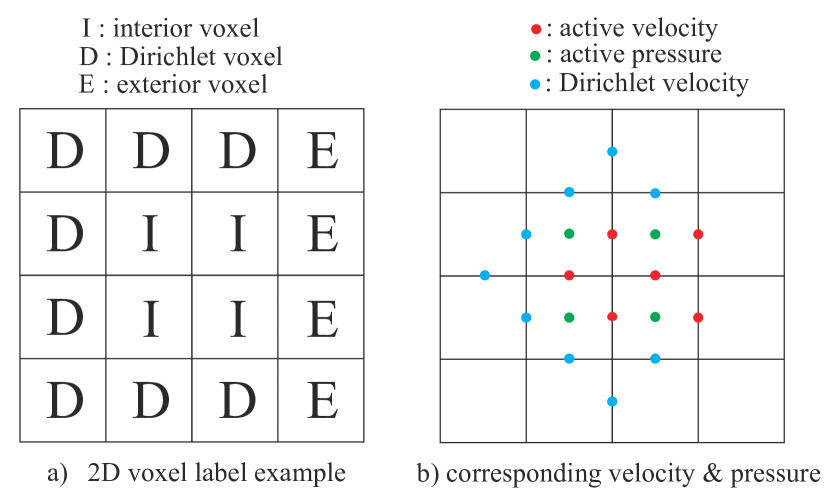
Figure 5: 2D Discrete Domain Example

6 Numerical experiments

In this section, we present the results of our numerical experiments, which compare the performance of our method with the pure multigrid method under different boundary conditions. The fluid viscosity is set to $\eta=10^{-3}m^{2}/s$, and $\gamma=10^{-3}$. To enhance the efficiency of Vanka smoothing, we pre-factorize $3^{4}$ in 2D or $3^{6}$ in 3D local saddle point problems, based on whether neighboring cells are Dirichlet, exterior or interior. It’s direct to parallel addictive Vanka smoother, and an 8-color scheme is applied to parallel multiplicative Vanka smoother. All examples are implemented in C++ code, and we utilize Intel Pardiso and Eigen as the direct solvers for the bottom level of V-cycle and for solving local saddle-point problems in the Vanka smoother respectively. The experiments are performed on a computer with an Intel(R) Xeon(R) CPU E5-2650 v3 @ 2.30GHz and 128 GB of main memory. Paraview is used for postprocessing the results. In the following section, we’ll discuss the results in 2D examples and 3D examples separately.

6.1 2D Numerical Examples

In this subsection, we explore four 2D examples to assess the performance of our approach. Specifically, we examine the driven cavity example and Poiseuille flow around cylinder example to evaluate the convergence rates in comparison to pure multigrid methods. Additionally, the remaining two examples demonstrate the capability of our method to effectively handle more complex scenarios beyond the scope of pure multigrid methods.

6.1.1 Driven Cavity Example

The driven-cavity example is a well-established benchmark in the field of computational fluid. In the 2D scenario, the computational domain is a unit square, where no-slip boundary conditions are imposed on the left, right and bottom sides. While on the top side, a zero vertical velocity and a constant horizontal velocity of $u=1.0m/s$ are imposed. We use a $1024^{2}$ unit square as our computational domain and an 8-level multigrid as our preconditioner and solver. The solved velocity field with streamline and the convergence of pure multigrid on $\mathbf{\tilde{L}}$ and multigrid-preconditioned SQMR on $\mathbf{L}$ are shown in Fig. 6. The iterations are terminated when the relative residual goes below $10^{-8}$, and the legend indicates the type and number of smoothers used for the boundary and interior regions. We consistently apply a symmetric distributive Gauss-Seidel smoother only once in each V-cycle to the interior region. This approach significantly reduces the execution time per V-cycle, given that the boundary degrees of freedom are typically less than $3\%$ of the total degrees of freedom. Table. 1 provides more detailed information about the percentage of the number of boundary degrees of freedom.

The convergence plots reveal that our preconditioner achieves faster convergence compared to the pure multigrid method. Furthermore, the multiplicative Vanka smoother is more efficient than the addictive one, even when the latter is applied three times per V-cycle. The convergence rates of both multiplicative and addictive methods closely match the ideal scenario where a direct solver is employed for the boundary domains.

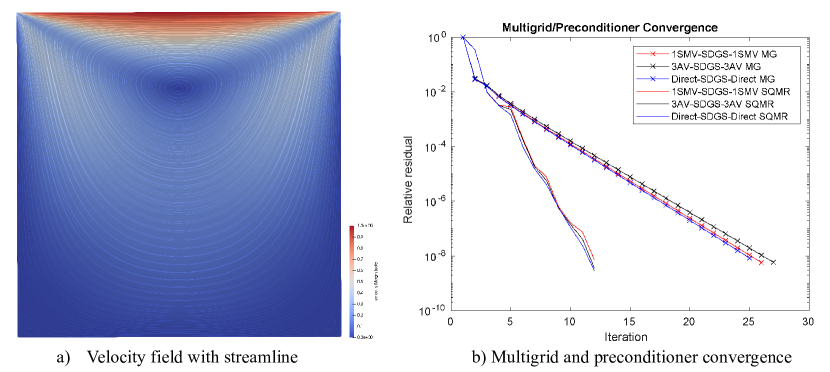
Figure 6: 2D $1024^{2}$ Driven Cavity Example

6.1.2 Poiseuille Flow around Cylinder Example

In the case of 2D Poiseuille flow, it represents the steady, laminar flow of an incompressible fluid through a channel driven by a pressure gradient. This flow scenario is commonly studied in benchmarks [34, 35], particularly with the presence of a cylindrical obstacle. In our 2D scenario, the channel dimensions are $2.2m\times 0.41m$, and a cylindrical obstacle is placed at position $(0.2m,0.2m)$ with a radius of $0.05m$. The inflow boundary conditions are described by

$$\begin{split}&u(0,y)=\frac{4\bar{u}y(H-y)}{H^{2}}\\ &v(0,y)=0\end{split}$$ (10)

where $\bar{u}=0.3m/s$ is the average horizontal velocity, and $H=0.41m$ is the width of the channel. On the outflow boundary, a homogeneous Neumann boundary condition is applied, while no-slippery boundary conditions are enforced on the top and bottom sides. The computational domain has dimensions $2200\times 410$, and a 6-level multigrid is used to solve the problem with $h=0.001m$. The partially solved velocity field and the convergence results are shown in Fig. 7, which shows that the effectiveness of symmetric multiplicative Vanka smoother. Besides that, the scalability of our multiplicative preconditioner and multigrid is demonstrated through various domain sizes in Fig. 8.

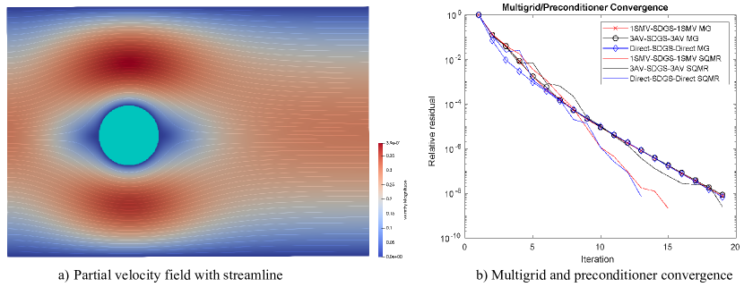
Figure 7: 2D $2200\times 410$ Poiseuille Flow around Cylinder Example

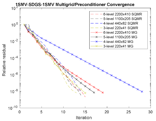
Figure 8: Convergence of 2D Cylinder Example in Different Dimensions

6.1.3 Poiseuille Flow around Hollow Square Example

In this example, we explore a more complex scenario involving Poiseuille flow around a hollow square obstacle. While pure multigrid suffices for simple applications, it may encounter divergence in more complicated scenarios. Here we use similar boundary conditions as those used in the cylindrical obstacle with $\bar{u}=1.0m/s$. The key difference lies in the presence of a hollow square obstacle, as depicted in Fig. 9 a). We perform our simulations on a $1024^{2}$ computational domain with an 8-level multigrid. It is observed that only the multiplicative preconditioner yields fast convergence, while the additive preconditioner and the pure multigrid method fail to converge. This behavior can be attributed to the close of the hollow square as the multigrid coarsens. Consequently, the solutions derived at coarser levels become increasingly inaccurate. However, when employed as a preconditioner, the multigrid method continues to guide SQMR towards successful convergence.

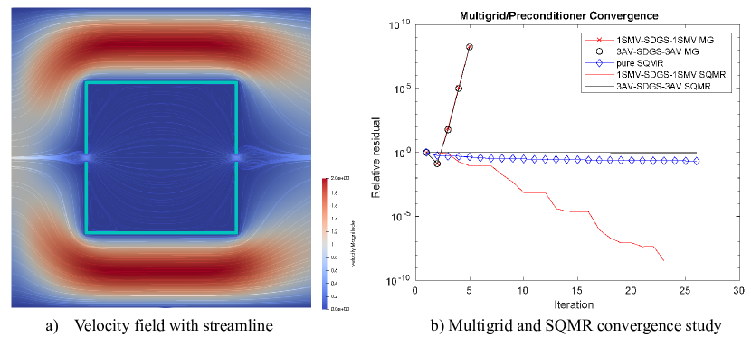
Figure 9: 2D $1024^{2}$ Poiseuille Flow around Hollow Square Example

6.1.4 Brancher Example

In the hollow square example, we explored the limitations of pure multigrid methods. Now we present a more practical example to emphasize the defects of pure multigrid methods and the reliability of multiplicative preconditioner. We keep the same boundary conditions and computational domain as those used in the hollow square obstacle. Instead of a single obstacle, we apply multiple rectangular obstacles near the outflow boundary to branch a single inflow into several outflows, forming a structure referred to as a ”brancher”. As shown in 10 b), our multiplicative preconditioner converges very fast. In contrast, the addictive preconditioner and the pure multigrid methods still struggle to converge. The hollow square example and the brancher example clearly show the effectiveness and reliability of the multiplicative preconditioner. This fact leads us to focus on the multiplicative methods in our upcoming 3D examples, without considering the addictive method. Additionally, we investigate the impact of the numbers of boundary smoothers on the convergence rate of multiplicative preconditioner in 11. The result indicates that increasing the numbers of boundary smoother leads to faster convergence rates.

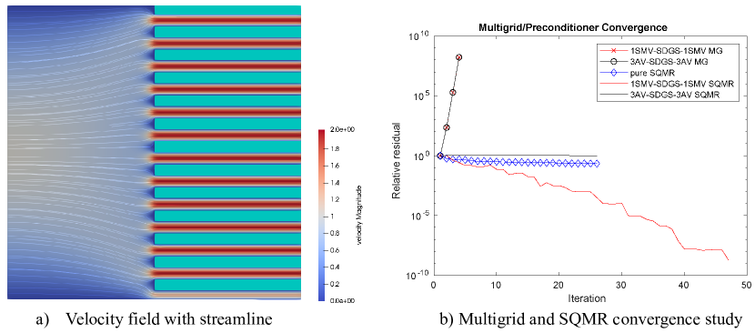
Figure 10: 2D $1024^{2}$ Brancher Example

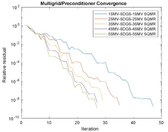
Figure 11: Convergence of 2D Brancher Example with Different Numbers of Boundary Smoothers

6.2 3D Numerical Examples

In this subsection, we consider four 3D examples using only multiplicative preconditioner and multigrid. Driven cavity example and Poiseuille flow with a cylindrical obstacle example show that our multigrid preconditioner achieves comparable convergence rates to pure multigrid methods. Then the last two examples highlight the capability of our approach to address more complicated scenarios beyond the capabilities of pure multigrid solvers.

6.2.1 Driven Cavity Example

3D driven cavity example is similar to its 2D version. In this case, we consider a unit cube instead of a unit square as our computational domain, applying no-slip boundary conditions to all sides except the top. The top side is subject to a constant horizontal velocity of $u=1.0m/s$. A 5-level multiplicative multigrid is used within a $128^{3}$ unit cube. We present the sliced velocity field and the convergence results in Fig. 12. We can see that our preconditioner converges faster compared to the multigrid method, closely resembling where the boundary domains are solved using a direct solver.

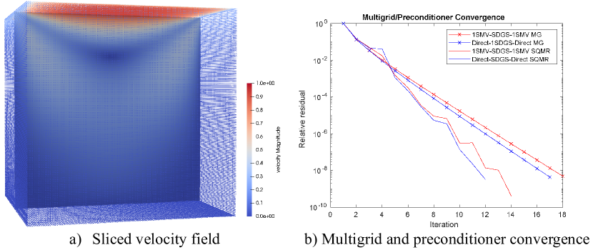
Figure 12: 3D $128^{3}$ Driven Cavity Example

6.2.2 Poiseuille Flow around Cylinder Example

In the 3D scenario, we also consider Poiseuille flow around a cylinder. The channel dimensions are $1.275m\times 0.41m\times 0.41m$, and a cylindrical obstacle is positioned along the $(0.5m,0.2m,z)$ axis with a radius of $0.05m$. The inflow boundary conditions are described as

$$\begin{split}&u(0,y,z)=\frac{16\bar{u}yz(H_{y}-y)(H_{z}-z)}{H^{4}}\\ &v(0,y,z)=0\\ &w(0,y,z)=0\end{split}$$ (11)

where $\bar{u}=0.45m/s$ represents the average horizontal velocity, and $H_{y}=H_{z}=0.41m$ are the inflow widths of the channel. Homogeneous Neumann boundary conditions are applied on the outflow boundary, while the surrounding sides are subject to no-slip conditions. The computational domain has dimensions of $255\times 82\times 82$, and a 4-level multigrid is used to solve the problem with $h=0.005m$. Fig. 13 b) shows the sliced velocity field and the convergence results. In this example, applying our symmetric multiplicative Vanka smoother only once does not yield convergence rates that match the ideal scenario where a direct solver is utilized on the boundary domains. Instead, we achieve the ideal convergence by increasing the number of smoothers applied to the boundary to 2.

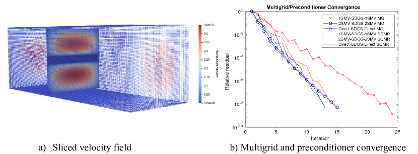
Figure 13: 3D $255\times 82\times 82$ Cylinder Example

6.2.3 Brancher Example

To highlight the effectiveness of our preconditioner, we present a 3D brancher example. We keep the same boundary condition as 3D Poiseuille flow around cylinder example except that we substitute cylinder to multiple cuboids near the outflow boundary and use $\bar{u}=1.0m/s$. A 5-level multigrid is used within a $128^{3}$ unit cube. The sliced velocity field and the convergence results are shown in Fig. 14. We can see that our multiplicative preconditioner can converge very fast but the pure SQMR and multigrid method fails. This example shows the advantage of our approach in 3D case.

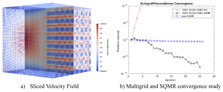
Figure 14: 3D $128^{3}$ Brancher Example

6.2.4 Porous Example

The final example we show is the porous example. In this example, we use the same boundary condition and computational domain as brancher example, but we use a porous layer as shown in Fig. 15 a) to replace the multiple cuboid obstacles. our multiplicative preconditioner exhibits rapid convergence, while the pure SQMR and multigrid methods prove ineffective, as illustrated in Fig. 15 b). This example further exemplifies the robustness and efficiency of our multiplicative preconditioner.

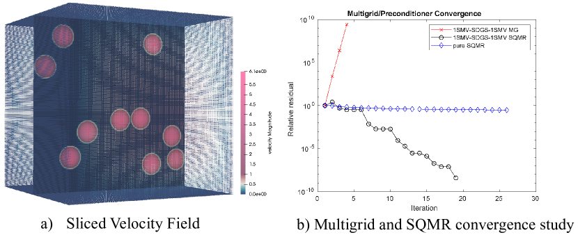
Figure 15: 3D $128^{3}$ Brancher Example

2D examples	#total degrees of freedom	#boundary degrees of freedom	boundary percentage
$1024^{2}$ Driven Cavity	3143680	12272	0.38%
$2200\times 410$ Cylinder	2680020	18493	0.69%
$1100\times 205$ Cylinder	669372	9243	1.38%
$440\times 82$ Cylinder	106812	3693	3.45%
$220\times 41$ Cylinder	26580	1843	6.93%
$1024^{2}$ Hollow Square	3463768	29305	0.85%
$1024^{2}$ Brancher	2546560	61077	2.39%
3D examples	#total degrees of freedom	#boundary degrees of freedom	boundary percentage
$128^{3}$ Driven Cavity	8339456	385580	4.62%
$255\times 82\times 82$ Cylinder	6788860	425856	6.27%
$128^{3}$ Brancher	8013824	1119980	13.98%
$128^{3}$ Porous	9156798	614304	6.71%

Table 1: The numbers of total and boundary degrees of freedom

7 Conclusions

In this work, we propose and evaluate a novel multigrid preconditioner for solving the Stokes equations in both 2D and 3D scenarios. Our approach leverages the strengths of symmetric distributive smoother and Vanka smoother, which are well-suited for handling interior and boundary regions respectively. By combining these smoothers carefully, we achieve an efficient symmetric multigrid precondition which can be used by the SQMR method. Our numerical experiments in 2D and 3D have demonstrated the advantages of our approach. It not only gets the comparable convergence rates as pure multigrid methods, but also maintains fast convergence even when pure multigrid methods struggle with divergence. The application of our preconditioner as a robust and reliable solver, particularly in challenging 3D cases, shows its potential to significantly enhance the efficiency of solving the Stokes equations. Our future endeavors will focus on GPU acceleration to enhance the scalability of our methods, allowing for the efficient resolution of larger-scale problems.

Appendix A Symmetry proof for symmetric distributive Gauss-Seidel

Lemma 1.

Consider a sequence $\mathbf{x}^{(k+1)}=\mathbf{A}\mathbf{x}^{(k)}+\mathbf{b}$ with $\mathbf{x}^{(0)}=\mathbf{0}$. The general formula is $\mathbf{x}^{(n)}=\sum_{i=0}^{n-1}\mathbf{A}^{i}\mathbf{b}$.

It’s obvious by using mathematical induction. ∎

Theorem 1.

In symmetric DGS smoother, when $\mathbf{L}$ is symmetric and $\mathbf{x}^{(0)}=\mathbf{0}$, then $\mathbf{x}^{(n)}=\mathbf{C}\mathbf{x}^{(0)}$ and $\mathbf{C}$ is a symmetric matrix.

Splitting $\mathbf{L}=\mathbf{G}+\mathbf{H}$ with a lower triangular matrix and a strictly upper triangular matrix, GS can be written as

$$\mathbf{x}^{(k+1)}=\mathbf{x}^{(k)}+\mathbf{G}^{-1}(\mathbf{b}-\mathbf{L}\mathbf{x}^{(k)})$$ (12)

After introducing the distributive preconditioner $\mathbf{M}$ and defining $\mathbf{\tilde{G}}$ and $\mathbf{\tilde{H}}$ as the lower and strictly upper triangular part of $\mathbf{L}\mathbf{M}$ instead of $\mathbf{L}$, the distributive GS can be written as

$$\mathbf{x}^{(k+1)}=\mathbf{x}^{(k)}+\mathbf{M}\mathbf{\tilde{G}}^{-1}(\mathbf{b}-\mathbf{L}\mathbf{x}^{(k)})$$ (13)

For the symmetric DGS smoother, the smoothing step can be written as

$$\begin{split}&\mathbf{x}^{(k+\frac{1}{2})}=\mathbf{x}^{(k)}+\mathbf{M}\mathbf{\tilde{G}}^{-1}(\mathbf{b}-\mathbf{L}\mathbf{x}^{(k)})\\ &\mathbf{x}^{(k+1)}=\mathbf{x}^{(k+\frac{1}{2})}+\mathbf{\tilde{G}}^{-T}\mathbf{M}^{T}(\mathbf{b}-\mathbf{L}\mathbf{x}^{(k+\frac{1}{2})})\end{split}$$ (14)

Substitute the first equation in Eq. 14 into the second one and denote $\mathbf{P}=\mathbf{M}\mathbf{\tilde{G}}^{-1}+\mathbf{\tilde{G}}^{-T}\mathbf{M}^{T}-\mathbf{\tilde{G}}^{-T}\mathbf{M}^{T}\mathbf{L}\mathbf{M}\mathbf{\tilde{G}}^{-1}$, we can get

$$\mathbf{x}^{(k+1)}=(\mathbf{I}-\mathbf{P}\mathbf{L})\mathbf{x}^{(k)}+\mathbf{P}\mathbf{b}$$ (15)

By using Lemma 1, the general formula of $\mathbf{x}^{(n)}$ is

$$\mathbf{x}^{(n)}=\sum_{i=0}^{n-1}(\mathbf{I}-\mathbf{P}\mathbf{L})^{i}\mathbf{P}\mathbf{b}=\sum_{i=0}^{n-1}\sum_{j=0}^{i}{i\choose j}(-\mathbf{P}\mathbf{L})^{i}\mathbf{P}\mathbf{b}=\mathbf{C}\mathbf{b}$$ (16)

Since $(-\mathbf{P}\mathbf{L})^{i}\mathbf{P}$ is always symmetric when $\mathbf{L}$ and $\mathbf{P}$ are symmetric, $\mathbf{C}$ is symmetric. ∎

Appendix B Symmetry proof for addictive Vanka smoother

Theorem 2.

In additive Vanka smoother, when $\mathbf{L}$ is symmetric and $\mathbf{x}^{(0)}=\mathbf{0}$, $\mathbf{x}^{(n)}=\mathbf{C}\mathbf{x}^{(0)}$ and $\mathbf{C}$ is a symmetric matrix.

We know that the series of addictive Vanka smoother can be written as

$$\mathbf{x}^{(k+1)}=\mathbf{x}^{(k)}+\mathbf{S}_{AV}(\mathbf{b}-\mathbf{L}\mathbf{x}^{(k)})=(\mathbf{I}-\mathbf{S}_{AV}\mathbf{L})\mathbf{x}^{(k)}+\mathbf{S}_{AV}\mathbf{b}$$ (17)

By using Lemma 1, the general formula of $\mathbf{x}^{(n)}$ is

$$\mathbf{x}^{(n)}=\sum_{i=0}^{n-1}(\mathbf{I}-\mathbf{S}_{AV}\mathbf{L})^{i}\mathbf{S}_{AV}\mathbf{b}=\sum_{i=0}^{n-1}\sum_{j=0}^{i}{i\choose j}(-\mathbf{S}_{AV}\mathbf{L})^{i}\mathbf{S}_{AV}\mathbf{b}=\mathbf{C}\mathbf{b}$$ (18)

Since $(-\mathbf{S}_{AV}\mathbf{L})^{i}\mathbf{S}_{AV}$ is always symmetric when $\mathbf{L}$ and $\mathbf{S}_{AV}$ are symmetric, $\mathbf{C}$ is symmetric. ∎

Appendix C Symmetry proof for symmetric multiplicative Vanka smoother

Theorem 3.

In symmetric multiplicative Vanka smoother, when $\mathbf{L}$ is symmetric and $\mathbf{x}^{(0)}=\mathbf{0}$, then $\mathbf{x}^{(n)}=\mathbf{C}\mathbf{x}^{(0)}$ and $\mathbf{C}$ is a symmetric matrix.

We know that the series of multiplicative Vanka smoother can be written as

$$\mathbf{x}^{(k+1)}=\mathbf{x}^{(k)}+\mathbf{S}_{MV}(\mathbf{b}-\mathbf{L}\mathbf{x}^{(k)})=(\mathbf{I}-\mathbf{S}_{MV}\mathbf{L})\mathbf{x}^{(k)}+\mathbf{S}_{MV}\mathbf{b}$$ (19)

For the symmetric multiplicative Vanka smoother, the smoothing step can be written as

$$\begin{split}&\mathbf{x}^{(k+\frac{1}{2})}=(\mathbf{I}-\mathbf{S}_{MV}^{(1)}\mathbf{L})\mathbf{x}^{(k)}+\mathbf{S}_{MV}^{(1)}\mathbf{b}\\ &\mathbf{x}^{(k+1)}=(\mathbf{I}-\mathbf{S}_{MV}^{(2)}\mathbf{L})\mathbf{x}^{(k)}+\mathbf{S}_{MV}^{(2)}\mathbf{b}\end{split}$$ (20)

where $\mathbf{S}_{MV}^{(1)}$ is solving in the order from domain $D_{1}$ to $D_{n}$, and $\mathbf{S}_{MV}^{(2)}$ is solving in the order from domain $D_{n}$ to $D_{1}$. Before we prove that this smoother is symmetric, let’s prove that $\mathbf{S}_{MV}^{(2)}=(\mathbf{S}_{MV}^{(1)})^{T}$. Denoting that $\mathbf{K}_{i}=\mathbf{C}_{i}^{T}(\mathbf{C}_{i}\mathbf{L}\mathbf{C}_{i}^{T})^{-1}\mathbf{C}_{i}$, We can rewrite the transpose of $\mathbf{S}_{MV}^{(1)}$ as

$$\begin{split}(\mathbf{S}_{MV}^{(1)})^{T}&=([\mathbf{I}-\prod_{i=1}^{n}(\mathbf{I}-\mathbf{K}_{i}\mathbf{L})]\mathbf{L}^{-1})^{T}=\mathbf{L}^{-1}[\mathbf{I}-\prod_{i=1}^{n}(\mathbf{I}-\mathbf{K}_{i}\mathbf{L})]^{T}\\ &=\mathbf{L}^{-1}-\mathbf{L}^{-1}\prod_{i=n}^{1}(\mathbf{I}-\mathbf{L}\mathbf{K}_{i})=\mathbf{L}^{-1}-[\prod_{i=n}^{1}(\mathbf{I}-\mathbf{K}_{i}\mathbf{L})]\mathbf{L}^{-1}\\ &=[\mathbf{I}-\prod_{i=n}^{1}(\mathbf{I}-\mathbf{K}_{i}\mathbf{L})]\mathbf{L}^{-1}=\mathbf{S}_{MV}^{(2)}\end{split}$$ (21)

Substitute the first equation in Eq. 20 into the second one and denote $\mathbf{P}=\mathbf{S}_{MV}^{(1)}+[\mathbf{S}_{MV}^{(1)}]^{T}-[\mathbf{S}_{MV}^{(1)}]^{T}\mathbf{L}\mathbf{S}_{MV}^{(1)}$, we can get

$$\mathbf{x}^{(k+1)}=(\mathbf{I}-\mathbf{P}\mathbf{L})\mathbf{x}^{(k)}+\mathbf{P}\mathbf{b}$$ (22)

By using Lemma 1, the general formula of $\mathbf{x}^{(n)}$ is

$$\mathbf{x}^{(n)}=\sum_{i=0}^{n-1}(\mathbf{I}-\mathbf{P}\mathbf{L})^{i}\mathbf{P}\mathbf{b}=\sum_{i=0}^{n-1}\sum_{j=0}^{i}{i\choose j}(-\mathbf{P}\mathbf{L})^{i}\mathbf{P}\mathbf{b}=\mathbf{C}\mathbf{b}$$ (23)

Since $(-\mathbf{P}\mathbf{L})^{i}\mathbf{P}$ is always symmetric when $\mathbf{L}$ and $\mathbf{P}$ are symmetric, $\mathbf{C}$ is symmetric. ∎

Appendix D Symmetry proof for symmetric integration of smoother

Lemma 2.

Consider a sequence $\mathbf{x}^{(k+1)}=\mathbf{A}\mathbf{x}^{(k)}+\mathbf{b}$. The general formula is $\mathbf{x}^{(n)}=\mathbf{A}^{n}\mathbf{x}^{(0)}+\sum_{i=0}^{n-1}\mathbf{A}^{i}\mathbf{b}$.

It’s obvious by using mathematical induction. ∎

Theorem 4.

For smoother shown in Alg. 3, when $\mathbf{L}$ is symmetric and $\mathbf{x}^{(0)}=\mathbf{0}$, then $\mathbf{x}^{(n)}=\mathbf{C}\mathbf{x}^{(0)}$ and $\mathbf{C}$ is a symmetric matrix.

Since we decouple the unknowns into two sets $V_{1}$ and $V_{2}$, we can reorder our system equations into

$$\mathbf{L}\mathbf{x}=\begin{pmatrix}\mathbf{L}_{11}&\mathbf{L}_{12}\\ \mathbf{L}_{21}&\mathbf{L}_{22}\\ \end{pmatrix}\begin{pmatrix}\mathbf{x}_{1}\\ \mathbf{x}_{2}\\ \end{pmatrix}=\begin{pmatrix}\mathbf{b}_{1}\\ \mathbf{b}_{2}\\ \end{pmatrix}=\mathbf{b}$$ (24)

where $x_{1}$ and $x_{2}$ represent unknowns for $V_{1}$ and $V_{2}$ separately.

For symmetric Vanka smoothing, it can be seen as solving the system

$$\mathbf{L}_{11}\mathbf{x}_{1}=\mathbf{b}_{1}-\mathbf{L}_{12}\mathbf{x}_{2}$$ (25)

And for symmetric distributive smoothing, it can be seen as solving the system

$$\mathbf{L}_{22}\mathbf{x}_{2}=\mathbf{b}_{2}-\mathbf{L}_{21}\mathbf{x}_{1}$$ (26)

For the first symmetric Vanka smoothing, $\mathbf{x}^{(0)}=\mathbf{0}$. By Theorem 2 or 3, we know that $[\mathbf{x}_{1},\mathbf{x}_{2}]^{T}=[\mathbf{C}_{1}\mathbf{b}_{1},\mathbf{0}]^{T}$ after smoothing, where $\mathbf{C}_{1}$ has the form $\sum_{i=0}^{n-1}\sum_{j=0}^{i}{i\choose j}(-\mathbf{P}\mathbf{L})^{i}\mathbf{P}\mathbf{b}$ with some symmetric matrix $\mathbf{P}$.

For the symmetric Vanka smoothing, $\mathbf{x}^{(0)}=[\mathbf{C}_{1}\mathbf{b}_{1},\mathbf{0}]^{T}$. By Theorem 1, we know that $[\mathbf{x}_{2},\mathbf{x}_{2}]^{T}=[\mathbf{C}_{1}\mathbf{b}_{1},\mathbf{C}_{2}(\mathbf{b}_{2}-\mathbf{L}_{21}\mathbf{C}_{1}\mathbf{b}_{1})]^{T}$ after smoothing, where $\mathbf{C}_{2}$ is also some symmetric matrix.

For the second symmetric Vanka smoothing, $\mathbf{x}^{(0)}=[\mathbf{C}_{1}\mathbf{b}_{1},\mathbf{C}_{2}(\mathbf{b}_{2}-\mathbf{L}_{21}\mathbf{C}_{1}\mathbf{b}_{1})]^{T}$. By Lemma 2 and Eq. 22, we know that

$$\begin{pmatrix}\mathbf{x}_{1}\\ \mathbf{x}_{2}\\ \end{pmatrix}=\begin{pmatrix}\mathbf{C}_{1}(\mathbf{b}_{1}-\mathbf{L}_{12}\mathbf{C}_{2}(\mathbf{b}_{2}-\mathbf{L}_{21}\mathbf{C}_{1}\mathbf{b}_{1}))+(\mathbf{I}-\mathbf{P}\mathbf{L})^{n}\mathbf{C}_{1}\mathbf{b}_{1}\\ \mathbf{C}_{2}(\mathbf{b}_{2}-\mathbf{L}_{21}\mathbf{C}_{1}\mathbf{b}_{1})\end{pmatrix}$$ (27)

after smoothing. And we can rewrite it in the matrix form

$$\begin{split}\begin{pmatrix}\mathbf{x}_{1}\\ \mathbf{x}_{2}\\ \end{pmatrix}&=\begin{pmatrix}\mathbf{C}_{1}+\mathbf{C}_{1}\mathbf{L}_{12}\mathbf{C}_{2}\mathbf{L}_{21}\mathbf{C}_{1}+(\mathbf{I}-\mathbf{P}\mathbf{L})^{n}\mathbf{C}_{1}&-\mathbf{C}_{1}\mathbf{L}_{12}\mathbf{C}_{2}\\ -\mathbf{C}_{2}\mathbf{L}_{21}\mathbf{C}_{1}&\mathbf{C}_{2}\\ \end{pmatrix}\begin{pmatrix}\mathbf{b}_{1}\\ \mathbf{b}_{2}\\ \end{pmatrix}\\ &=\mathbf{C}\mathbf{b}\\ \end{split}$$ (28)

Since $\mathbf{C}_{1}$ has the form $\sum_{i=0}^{n-1}\sum_{j=0}^{i}{i\choose j}(-\mathbf{P}\mathbf{L})^{i}\mathbf{P}\mathbf{b}$ with some symmetric matrix $\mathbf{P}$, $(\mathbf{I}-\mathbf{P}\mathbf{L})^{n}\mathbf{C}_{1}$ is still symmetric. Therefore, $\mathbf{C}$ is symmetric. ∎

Acknowledgements
This work was supported in part by NSF Grant IIS-2106768.

Declaration of generative AI and AI-assisted technologies in the writing process
During the preparation of this work the author(s) used chatgpt in order to polish the sentences. After using this tool/service, the author(s) reviewed and edited the content as needed and take(s) full responsibility for the content of the publication.

References

- [1] R. W. Freund, N. M. Nachtigal, A new krylov-subspace method for symmetric indefinite linear systems, Tech. rep., Oak Ridge National Lab., TN (United States) (1994).
- [2] H. C. Elman, Preconditioners for saddle point problems arising in computational fluid dynamics, Applied Numerical Mathematics 43 (1-2) (2002) 75–89.
- [3] A. C. de Niet, F. W. Wubs, Two preconditioners for saddle point problems in fluid flows, International Journal for Numerical Methods in Fluids 54 (4) (2007) 355–377.
- [4] C. Farhat, A saddle-point principle domain decomposition method for the solution of solid mechanics problems, Domain Decomposition Methods for Partial Differential Equations (1992) 271–292.
- [5] A. Franceschini, N. Castelletto, M. Ferronato, Block preconditioning for fault/fracture mechanics saddle-point problems, Computer Methods in Applied Mechanics and Engineering 344 (2019) 376–401.
- [6] E. G. Phillips, J. N. Shadid, E. C. Cyr, H. C. Elman, R. P. Pawlowski, Block preconditioners for stable mixed nodal and edge finite element representations of incompressible resistive mhd, SIAM Journal on Scientific Computing 38 (6) (2016) B1009–B1031.
- [7] U. Trottenberg, C. W. Oosterlee, A. Schuller, Multigrid, Elsevier, 2000.
- [8] C. W. Oosterlee, F. J. G. Lorenz, Multigrid methods for the stokes system, Computing in science & engineering 8 (6) (2006) 34–43.
- [9] H. C. Elman, G. H. Golub, Inexact and preconditioned uzawa algorithms for saddle point problems, SIAM Journal on Numerical Analysis 31 (6) (1994) 1645–1661.
- [10] D. Braess, R. Sarazin, An efficient smoother for the stokes problem, Applied Numerical Mathematics 23 (1) (1997) 3–19.
- [11] S. P. Vanka, Block-implicit multigrid solution of navier-stokes equations in primitive variables, Journal of Computational Physics 65 (1) (1986) 138–158.
- [12] C. Bacuta, P. S. Vassilevski, S. Zhang, A new approach for solving stokes systems arising from a distributive relaxation method, Numerical Methods for Partial Differential Equations 27 (4) (2011) 898–914.
- [13] M. Wang, L. Chen, Multigrid methods for the stokes equations using distributive gauss–seidel relaxations based on the least squares commutator, Journal of Scientific Computing 56 (2013) 409–431.
- [14] L. Chen, X. Hu, M. Wang, J. Xu, A multigrid solver based on distributive smoother and residual overweighting for oseen problems, Numerical Mathematics: Theory, Methods and Applications 8 (2) (2015) 237–252.
- [15] J. Maitre, F. Musy, P. Nigon, A fast solver for the stokes equations using multigrid with a uzawa smoother, in: Advances in Multi-Grid Methods: Proceedings of the conference held in Oberwolfach, December 8 to 13, 1984, Springer, 1985, pp. 77–83.
- [16] P. Luo, C. Rodrigo, F. J. Gaspar, C. W. Oosterlee, Uzawa smoother in multigrid for the coupled porous medium and stokes flow system, SIAM journal on Scientific Computing 39 (5) (2017) S633–S661.
- [17] S. V. Patankar, D. B. Spalding, A calculation procedure for heat, mass and momentum transfer in three-dimensional parabolic flows, in: Numerical prediction of flow, heat transfer, turbulence and combustion, Elsevier, 1983, pp. 54–73.
- [18] Y. He, S. P. MacLachlan, Local fourier analysis of block-structured multigrid relaxation schemes for the stokes equations, Numerical Linear Algebra with Applications 25 (3) (2018) e2147.
- [19] J. H. Adler, T. R. Benson, E. C. Cyr, S. P. MacLachlan, R. S. Tuminaro, Monolithic multigrid methods for two-dimensional resistive magnetohydrodynamics, SIAM Journal on Scientific Computing 38 (1) (2016) B1–B24.
- [20] S. Saberi, G. Meschke, A. Vogel, A restricted additive vanka smoother for geometric multigrid, Journal of Computational Physics 459 (2022) 111123.
- [21] S. Franco, C. Rodrigo, F. Gaspar, M. Pinto, A multigrid waveform relaxation method for solving the poroelasticity equations, Computational and Applied Mathematics 37 (2018) 4805–4820.
- [22] Analysis of a multigrid strokes solver, Applied Mathematics and Computation 35 (3) (1990) 291–303.
- [23] A. Brandt, O. E. Livne, Multigrid Techniques: 1984 Guide with Applications to Fluid Dynamics, Revised Edition, SIAM, 2011.
- [24] I. Parsons, J. Hall, The multigrid method in solid mechanics: part ii—practical applications, International Journal for Numerical Methods in Engineering 29 (4) (1990) 739–753.
- [25] O. Tatebe, The multigrid preconditioned conjugate gradient method, in: NASA. Langley Research Center, The Sixth Copper Mountain Conference on Multigrid Methods, Part 2, 1993.
- [26] Y. Saad, M. H. Schultz, Gmres: A generalized minimal residual algorithm for solving nonsymmetric linear systems, SIAM Journal on scientific and statistical computing 7 (3) (1986) 856–869.
- [27] S. Oliveira, Y. Deng, Preconditioned krylov subspace methods for transport equations, Progress in Nuclear Energy 33 (1-2) (1998) 155–174.
- [28] C. Oosterlee, T. Washio, On the use of multigrid as a preconditioner, in: Proceedings of Ninth International Conference on Domain Decomposition Methods, Citeseer, 1996, pp. 441–448.
- [29] A. Ramage, A multigrid preconditioner for stabilised discretisations of advection–diffusion problems, Journal of computational and applied mathematics 110 (1) (1999) 187–203.
- [30] M. Anselmann, M. Bause, Efficiency of local vanka smoother geometric multigrid preconditioning for space-time finite element methods to the navier–stokes equations, PAMM 23 (1) (2023) e202200088.
- [31] C. C. Paige, M. A. Saunders, Solution of sparse indefinite systems of linear equations, SIAM journal on numerical analysis 12 (4) (1975) 617–629.
- [32] K. Stüben, U. Trottenberg, Multigrid methods: Fundamental algorithms, model problem analysis and applications, in: Multigrid Methods: Proceedings of the Conference Held at Köln-Porz, November 23–27, 1981, Springer, 2006, pp. 1–176.
- [33] J. Schöberl, W. Zulehner, On schwarz-type smoothers for saddle point problems, Numerische Mathematik 95 (2) (2003) 377–399.
- [34] M. Schafer, S. Turek, F. Durst, E. Krause, R. Rannacher, Benchmark computations of laminar flow around a cylinder, Notes on numerical fluid mechanics 52 (1996) 547–566.
- [35] X. Nicolas, M. Medale, S. Glockner, S. Gounand, Benchmark solution for a three-dimensional mixed-convection flow, part 1: Reference solutions, Numerical Heat Transfer, Part B: Fundamentals 60 (5) (2011) 325–345.