Fitting a manifold to data in the presence of large noise

Abstract

We assume that $\mathcal{M}_{0}$ is a $d$-dimensional $C^{2,1}$-smooth submanifold of $\mathbb{R}^{n}$. Let $K_{0}$ be the convex hull of $\mathcal{M}_{0},$ and $B^{n}_{1}(0)$ be the unit ball. We assume that

$$\mathcal{M}_{0}\subseteq\partial K_{0}\subseteq B^{n}_{1}(0).$$ (1)

We also suppose that $\mathcal{M}_{0}$ has volume ($d$-dimensional Hausdorff measure) less or equal to $V$, reach (i.e., normal injectivity radius) greater or equal to $\tau$. Moreover, we assume that $\mathcal{M}_{0}$ is $R$-exposed, that is, tangent to every point $x\in\mathcal{M}$ there is a closed ball in $\mathbb{R}^{n}$ of the radius $R$ that contains $\mathcal{M}$.

Let $x_{1},\dots,x_{N}$ be independent random variables sampled from uniform distribution on $\mathcal{M}_{0}$ and $\zeta_{1},\dots,\zeta_{N}$ be a sequence of i.i.d Gaussian random variables in $\mathbb{R}^{n}$ that are independent of $x_{1},\dots,x_{N}$ and have mean zero and covariance $\sigma^{2}I_{n}.$ We assume that we are given the noisy sample points $y_{i}$, given by

$${y_{i}=x_{i}+\zeta_{i},\quad\hbox{ for }i=1,2,\dots,N.}$$

Let ${\epsilon},\eta>0$ be real numbers and $k\geq 2$. Given points $y_{i}$, $i=1,2,\dots,N$, we produce a $C^{k}$-smooth function which zero set is a manifold $\mathcal{M}_{\color[rgb]{0,0,0}rec}\subseteq\mathbb{R}^{n}$ such that the Hausdorff distance between $\mathcal{M}_{\color[rgb]{0,0,0}rec}$ and $\mathcal{M}_{0}$ is at most ${\epsilon}$ and $\mathcal{M}_{\color[rgb]{0,0,0}rec}$ has reach that is bounded below by ${c\tau}/{d{}^{6}}$ with probability at least $1-\eta.$ Assuming $d<c\sqrt{\log\log n}$ and all the other parameters are positive constants independent of $n$, the number of the needed arithmetic operations is polynomial in $n$. In the present work, at the cost of introducing a new condition that $\mathcal{M}_{0}$ is $R$-exposed and requiring that $\mathcal{M}_{0}$ be $C^{2,1}$-smooth rather than $C^{2},$ we allow the noise magnitude $\sigma$ to be an arbitrarily large constant, thus overcoming a drawback of the previous work [45].

1 Introduction

One of the main challenges in high dimensional data analysis is dealing with the exponential growth of the computational and sample complexity of generic inference tasks as a function of dimension, a phenomenon termed “the curse of dimensionality”. One intuition that has been put forward to diminish the impact of this curse is that high dimensional data tend to lie near a low dimensional submanifold of the ambient space. Algorithms and analyses that are based on this hypothesis constitute the subfield of learning theory known as manifold learning. In the present work, we give a solution to the following question from manifold learning. Suppose data is drawn independently, identically distributed (i.i.d) from a measure supported on a low dimensional $C^{2,1}$ manifold $\mathcal{M}_{0}$ whose reach is at least $\tau$, and corrupted by a large amount of (i.i.d) Gaussian noise. How can can we produce a manifold $\mathcal{M}_{\color[rgb]{0,0,0}rec}$ whose Hausdorff distance to $\mathcal{M}_{0}$ is small and whose reach is not much smaller than $\tau$?

This question is an instantiation of the problem of understanding the geometry of data. To give a specific real-world example, the issue of denoising noisy Cryo-electron microscopy (Cryo-EM) images falls into this general category. Cryo-EM images are X-ray images of three-dimensional macromolecules, e.g. viruses, possessing an arbitrary orientation. The space of orientations is in correspondence with the Lie group $SO_{3}(\mathbb{R})$, which is only three dimensional. However, the ambient space of greyscale images on $[0,1]^{2}$ can be identified with an infinite dimensional subspace of $\mathcal{L}^{2}([0,1]^{2})$, which gets projected down to a finite $n-$dimensional subspace indexed by $n=k\times k$ pixels, where $k$ is large. through the process of dividing $[0,1]^{2}$ into pixels. When the molecule is not invariant under any nontrivial rigid body rotations, the noisy Cryo-EM X-ray images lie approximately on an embedding of a compact $3-$dimensional manifold in a very high dimensional space. If the errors are modelled as being Gaussian, then fitting a manifold to the data can subsequently allow us to project the data onto this output manifold. Due to the large codimension and small dimension of the true manifold, the noise vectors are almost perpendicular to the true manifold and the projection would effectively denoise the data. The immediate rationale behind having a good lower bound on the reach is that this implies good generalization error bounds with respect to squared loss (See Theorem 1 in [46]). Another reason why this is desirable is that the projection map onto such a manifold is Lipschitz within a tube of the manifold of radius equal to $c$ times the reach for any $c$ less than $1$.

LiDAR (Light Detection and Ranging) also produces point cloud data for which the methods of this paper could be applied.

1.1 A note on constants

In the following sections, we will denote positive absolute constants by $c,C,C_{1},C_{2},\overline{c}_{1}$ etc. These constants are universal and positive, but their precise value may differ from occurrence to occurrence. Also, for a natural number $n$, we will use $[n]$ to denote the set $\{1,2,\dots,n\}.$

1.2 The model

We assume that $\mathcal{M}_{0}$ is a $d$-dimensional $C^{2,1}$-smooth submanifold of $\mathbb{R}^{n}$. Let $K_{0}$ be the convex hull of $\mathcal{M}_{0}$. We assume that

$$\mathcal{M}_{0}\subseteq\partial K_{0}\subseteq B^{n}_{1}(0).$$

We also suppose that $\mathcal{M}_{0}$ has volume ($d$-dimensional Hausdorff measure) less or equal to $V$, reach (i.e. normal injectivity radius) greater or equal to $\tau$. We denote this class of manifolds by $\mathcal{G}(d,n,V,\tau).$ Let $x_{1},\dots,x_{N}$ be a sequence of points chosen i.i.d at random from a probability measure $\mu$ that is proportional to the $d$-dimensional Hausdorff measure $\mathcal{H}^{d}_{\mathcal{M}_{0}}=\lambda_{\mathcal{M}_{0}}$ on $\mathcal{M}_{0}$.

Let $G_{\sigma}^{(n)}$ denote the Gaussian distribution supported on $\mathbb{R}^{n}$ whose density (Radon-Nikodym derivative with respect to the Lebesgue measure) at $x$ is

$$\pi_{G_{\sigma}^{(n)}}(x)=\left(\frac{1}{2\pi\sigma^{2}}\right)^{\frac{n}{2}}\exp\left(-\frac{\|x\|^{2}}{2\sigma^{2}}\right).$$ (2)

Let $\zeta_{1},\dots,\zeta_{N}$ be a sequence of i.i.d random variables independent of $x_{1},\dots,x_{N}$ having the distribution $G_{\sigma}^{(n)}$. We observe

$${y_{i}=x_{i}+\zeta_{i},\quad\hbox{ for }i=1,2,\dots,N.}$$ (3)

Note that the distribution of $y_{i}$ (for each $i$), is the convolution of $\mu$ and $G_{\sigma}^{(n)}$. This is denoted by $\mu*G_{\sigma}^{(n)}$. Let $\omega_{d}$ be the volume of a $d$ dimensional unit Euclidean ball.

We observe $y_{1},y_{2},\dots,y_{N}$ and in this paper produce an ${\epsilon}$-net of $\mathcal{M}_{0}$, where ${\epsilon}<<\tau.$ In Section 12, we indicate how earlier results described below can be used to generate an implicit description of the manifold using this ${\epsilon}$-net.

1.3 A survey of related work

Let $f:K\rightarrow\mathbb{R}$ be a function defined on a given (arbitrary) set $K\subset\mathbb{R}^{n}$, and let $m\geq 1$ be a given integer. The classical Whitney problem is the question whether $f$ extends to a function $F\in C^{m}(\mathbb{R}^{n})$ and if such an $F$ exists, what is the optimal $C^{m}$ norm of the extension. Furthermore, one is interested in the questions if the derivatives of $F$, up to order $m$, at a given point can be estimated, or if one can construct extension $F$ so that it depends linearly on $f$.

These questions go back to the work of H. Whitney [88, 89, 90] in 1934. In the decades since Whitney’s seminal work, fundamental progress was made by G. Glaeser [50], Y. Brudnyi and P. Shvartsman [14, 15, 16, 17, 18, 19] and [78, 79, 80], and E. Bierstone-P. Milman-W. Pawluski [11]. (See also N. Zobin [95, 96] for the solution of a closely related problem.)

The above questions have been answered in the last few years, thanks to work of E. Bierstone, Y. Brudnyi, C. Fefferman, P. Milman, W. Pawluski, P. Shvartsman and others, (see [11, 13, 14, 16, 17, 19, 35, 36, 37, 38, 39].) Along the way, the analogous problems with $C^{m}(\mathbb{R}^{n})$ replaced by $C^{m,\omega}(\mathbb{R}^{n})$, the space of functions whose $m^{th}$ derivatives have a given modulus of continuity $\omega$, (see [38, 39]), were also solved.

The solution of Whitney’s problems has led to a new algorithm for interpolation of data, due to C. Fefferman and B. Klartag [40, 41], where the authors show how to compute efficiently an interpolant $F(x),$ whose $C^{m}$ norm lies within a factor $C$ of least possible, where $C$ is a constant depending only on $m$ and $n.$

In traditional manifold learning, for instance, by using the ISOMAP algorithm introduced in the seminal paper [83], one often aims to map points $X_{j}$ to points $Y_{j}=F(X_{j})$ in an Euclidean space $\mathbb{R}^{m}$, where $m\geq n$ is as small as possible so that the Euclidean distances $\|Y_{j}-Y_{k}\|_{\mathbb{R}^{m}}$ are close to the intrinsic distances $d_{M}(X_{j},X_{k})$ and find a submanifold $\tilde{M}\subset\mathbb{R}^{m}$ that is close to the points $Y_{j}$. This method has turned out to be very useful, in particular in finding the topological manifold structure of the manifold $(M,g)$. It has been shown that when the original manifold $(M,g)$ has a vanishing Riemann curvature and satisfies certain convexity conditions, the manifold reconstructed by the ISOMAP approaches the original manifold as the number of the sample points tends to infinity (see the results in [21, 30, 31] for ISOMAP and [93] for the continuum version of ISOMAP). We note that for a general Riemannian manifold, the construction of a map $F:M\to\mathbb{R}^{m}$, for which the intrinsic metric of the embedded manifold $F(M)=\tilde{M}\subset\mathbb{R}^{m}$ is isometric to $(M,g)$ is a very difficult task numerically as it means finding a map, the existence of which is proved by the Nash embedding theorem (see [64, 65] and [84] on numerical techniques based on the Nash embedding theorem). We emphasize that the construction of an isometric embedding $f:M\to\mathbb{R}^{n}$ is outside of the context of the paper.

One can overcome the difficulties related to the construction of the Nash embedding by formulating the problem in a coordinate invariant way: Given the geodesic distances of points sampled from a Riemannian manifold $(M,g)$, construct a manifold $M^{*}$ with an intrinsic metric tensor $g^{*}$ so that the Lipschitz distance of $(M^{*},g^{*})$ to the original manifold $(M,g)$ is small. The construction of abstract manifolds from the distances of sampled data points has also been considered by Coifman and Lafon [27] and Coifman et al. [26] using “Diffusion Maps”, and by Belkin and Niyogi [6] using “EigenMaps”, where the data points are mapped to the values of the approximate eigenfunctions or diffusion kernels at the sample points. These methods construct a non-isometric embedding of the manifold $M$ into $\mathbb{R}^{m}$ with a sufficiently large $m$. This construction is continued in [62] by computing an approximation the metric tensor $g$ by using finite differences to find the Laplacian of the products of the local coordinate functions. In [44], we extend the results of [43] that deals with the question how a smooth manifold, that approximates a manifold $(M,g)$, can be constructed, when one is given the distances of the points of in a discrete subset $X$ of $M$ with small deterministic errors. In this paper we extend these results to two directions. First, the discrete set is randomly sampled and the distances have (possibly large) random errors. Second, we consider the case when some distance information is missing.

The question of fitting a manifold to data is of interest to data analysts and statisticians [1, 3, 23, 54, 47, 48, 57, 81, 91, 92]. We will focus our attention on results that provide an algorithm for describing a manifold to fit the data together with upper bounds on the sample complexity.

A work in this direction [49], building over [66] provides an upper bound on the Hausdorff distance between the output manifold and the true manifold equal to $O((\frac{\log N}{N})^{\frac{2}{n+8}})+{O}(\sigma^{2}\log(\sigma^{-1}))$. Note that in order to obtain a Hausdorff distance of $c{\epsilon}$, one needs more than ${\epsilon}^{-n/2}$ samples, where $n$ is the ambient dimension. This bound is exponential in $n$ and thus differs significantly from our results.

1.4 The case of small noise

In an earlier work [45], we gave a solution to the following question from manifold learning. Suppose data is drawn independently, identically distributed (i.i.d) from a measure supported on a low dimensional twice differentiable ($\mathcal{C}^{2}$) manifold $\mathcal{M}$ whose reach is $\geq\tau$, and corrupted by a small amount of (i.i.d) Gaussian noise. How can can we produce a manifold $\mathcal{M}_{\color[rgb]{0,0,0}rec}$ whose Hausdorff distance to $\mathcal{M}$ is small and whose reach is not much smaller than $\tau$?

Let $\zeta_{1},\dots,\zeta_{N}$ be a sequence of i.i.d random variables independent of $x_{1},\dots,x_{N}$ having the distribution $G_{\sigma}^{(n)}$. We observe

$${y_{i}=x_{i}+\zeta_{i},\quad\hbox{ for }i=1,2,\dots,N,}$$

and wish to construct a manifold $\mathcal{M}_{\color[rgb]{0,0,0}rec}$ close to $\mathcal{M}$ in Hausdorff distance but at the same time having a reach not much less than $\tau$. Note that the distribution of $y_{i}$ (for each $i$), is the convolution of $\mu$ and $G_{\sigma}^{(n)}$. This is denoted by $\mu*G_{\sigma}^{(n)}$. Let $\omega_{d}$ be the volume of a $d$ dimensional unit Euclidean ball. In [45], we supposed that

$$\sigma<r_{c}D^{-1/2},\quad\hbox{where }r_{c}:=cd^{-C}\tau,\ D=\min\left(n,\frac{V}{c^{d}\omega_{d}\beta^{d}}\right),\ \beta=\tau\sqrt{\frac{c^{d}\omega_{d}\tau^{d}}{V}},$$ (4)

and $\Delta\geq\frac{Cd\sigma^{2}}{\tau}.$ The points $y_{1},y_{2},\dots,y_{N}$ are observed and for $k\geq 3$, the algorithm produces a description of a $\mathcal{C}^{k}-$manifold $\mathcal{M}_{\color[rgb]{0,0,0}rec}$ such that the Hausdorff distance between $\mathcal{M}_{\color[rgb]{0,0,0}rec}$ and $\mathcal{M}$ is at most $\Delta$ and $\mathcal{M}_{\color[rgb]{0,0,0}rec}$ has reach that is bounded below by $\frac{c\tau}{d^{6}}$ with probability at least $1-\eta.$

1.5 New contributions

In the present work, we allow $\sigma$ to be an arbitrarily large constant, thus overcoming a drawback of the previous work from [45] mentioned above. On the other hand, our model is more restrictive in some ways; namely, we consider a $C^{2,1}$ manifold $\mathcal{M}$ rather than a $\mathcal{C}^{2}$ manifold, and require that the manifold underlying the data is $R$-exposed in the sense of Section 3. This means that, tangent to every point $x\in\mathcal{M}$ is a $n-1$-sphere of radius $R$, such that, the closed ball that it is the boundary of, contains $\mathcal{M}$.

The following is our main theorem.

Theorem 1.1.

Let the dimensions $d,n$, the noise level $\sigma$ and the geometric bounds $R,\Lambda,\tau,V$, see formulas (G1), (G2), and (G3) in Section 2.3, be such that that $\Lambda\geq\tau^{-2}$, see (18). Let the probability bound $\eta$ satisfy $0<\eta<\frac{1}{2}$. Moreover, let the accuracy parameter ${\epsilon}$ be such that ${\epsilon}<\beta^{2}/2$, see (46), where $\beta$ is given by (44) and (53). Assume that we are given noisy sample points $y_{1},\dots,y_{N}\in\mathbb{R}^{n}$, see (3), where $N$ satisfies

$$N\geq\tilde{\Omega}\left(\exp\left(\left(\frac{\sigma}{{\epsilon}\tau}\log\frac{V}{\tau^{d}}\right)^{2}\right)\log\left(\eta^{-1}\right)\right).$$ (5)

Then, our algorithm in Sections 11 and 12 produces the parameters of a function $F_{\color[rgb]{0,0,0}rec}$, see (148), such the manifold $\mathcal{M}_{\color[rgb]{0,0,0}rec}=\{x\in\mathbb{R}^{n}:\ F_{\color[rgb]{0,0,0}rec}(x)=0\}$ has a reach at least $\frac{C\tau}{d^{6}}$ and the Hausdorff distance of $\mathcal{M}_{\color[rgb]{0,0,0}rec}$ to $\mathcal{M}_{0}$ is less than ${\epsilon},$ with probability at least $1-\eta.$ Moreover, when $d<c\sqrt{\log\log n}$, the number of arithmetic operations in the algorithm is less than $n^{C_{0}}$, where $C_{0}$ depends only on $\sigma,R,\Lambda,\tau,V,\eta,{\epsilon}$.

2 Preliminaries

2.1 Notation for manifolds

• $\mathcal{M}$ is a closed $d$-submanifold of $E$, $p\in\mathcal{M}$, where $E$ is an $n$-dimensional Euclidean space which we identify with $\mathbb{R}^{n}.$

• $T_{p}\mathcal{M}$ denotes the tangent space to $\mathcal{M}$ at $p$, regarded a linear subspace of $\mathbb{R}^{n}$.

• $T_{p}^{\perp}\mathcal{M}=(T_{p}\mathcal{M})^{\perp}$ is the normal space, i.e., the orthogonal complement to $T_{p}\mathcal{M}$ in $\mathbb{R}^{n}$.

• $\mathcal{S}_{p}=\mathcal{S}_{p}^{\mathcal{M}}$ is the second fundamental form of $M$ at $p$. It is a symmetric bilinear map from $T_{p}\mathcal{M}\times T_{p}\mathcal{M}$ to $T_{p}^{\perp}\mathcal{M}$. To simplify the technical details in the sequel, we assume that $\mathcal{S}_{p}$ is extended to a symmetric bilinear map from $\mathbb{R}^{n}\times\mathbb{R}^{n}$ to $\mathbb{R}^{n}$ by setting $\mathcal{S}_{p}(v,w)=0$ whenever $v\in T_{p}^{\perp}\mathcal{M}$. The values of the extended $\mathcal{S}_{p}$ still belong to $T_{p}^{\perp}\mathcal{M}\subset\mathbb{R}^{n}$.

• For a linear subspace $X\subset\mathbb{R}^{n}$, we denote by $\Pi_{X}$ the orthogonal projection from $\mathbb{R}^{n}$ to $X$. When the manifold $\mathcal{M}$ is clear from context, we use notation $\Pi_{p}$ and $\Pi_{p}^{\perp}$, where $p\in M$, for the projections $\Pi_{T_{p}\mathcal{M}}$ and $\Pi_{T_{p}^{\perp}\mathcal{M}}$, respectively.

2.2 Notation for convex sets and cones

Figure 1: Outer normal cones for points on $\mathcal{M}\subseteq\partial K$. When $\mathcal{M}$ is a zero dimensional manifold corresponding to three noncollinear points, $K$ is a triangle and the outer normal cones are cones at the vertices of the triangle as depicted.

• $B_{r}(x)$, where $x\in\mathbb{R}^{n}$ and $r>0$, is the $r$-ball centered at $x$.

• $\operatorname{conv}(X)$, for $X\subset\mathbb{R}^{n}$, is the convex hull of $X$.

• A set $K\subset\mathbb{R}^{n}$ is a cone if $tx\in K$ whenever $x\in K$ and $t\geq 0$. All cones are linear cones, i.e., with apex at 0.

• $\operatorname{cone}(X)$ is the least cone containing $X$: $\operatorname{cone}X=\{tx\mid x\in X,t\geq 0\}$. One sees that the least convex cone containing $X$ can be obtained as

  $$\operatorname{conv}\operatorname{cone}(X)=\operatorname{cone}\operatorname{conv}(X)=\{\text{nonnegative linear combinations of points of $X$}\}.$$

• For a set $K\subset\mathbb{R}^{n}$, $K^{\circ}$ denotes the polar set:

  $$K^{\circ}=\{x\in\mathbb{R}^{n}:\forall y\in K,\ \langle x,y\rangle\leq 1\}$$

  If $K$ is a closed convex set and $0\in K$, then $K^{\circ\circ}=K$ by the Bipolar Theorem. If $K$ is a cone then the definition of $K^{\circ}$ can be simplified:

  $$K^{\circ}=\{x\in\mathbb{R}^{n}:\forall y\in K,\ \langle x,y\rangle\leq 0\}.$$

• For a closed convex set $K\subset\mathbb{R}^{n}$ and $p\in K$, the tangent cone of $K$ at $p$ is

  $$T_{K}(p)=\operatorname{cl}\operatorname{cone}(K-p)$$

  and the outward normal cone is

  $$N_{K}(p)=(T_{K}(p))^{\circ}=\{v\in\mathbb{R}^{n}:\forall x\in K,\ \langle v,x-p\rangle\leq 0\}.$$

• The distance between cones $K_{1}$ and $K_{2}$ is defined as the Hausdorff distance between their intersections with the unit ball:

  $$d_{CH}(K_{1},K_{2})=d_{H}(K_{1}\cap B_{1}(0),K_{2}\cap B_{1}(0))$$

  where $d_{H}$ is the Hausdorff distance.

2.3 Geometric bounds

We assume the following about the manifold $\mathcal{M}=\mathcal{M}^{d}\subset\mathbb{R}^{n}$.

1. The reach of $\mathcal{M}$ is bounded below by a constant $\tau>0$, and is $C^{2,1}$ thus belongs to $\mathcal{G}(d,n,V,\tau)$.

2. $\mathcal{M}$ is $R$-exposed for some constant $R>0$. The $R$-exposedness property is defined as follows: We say that a point $p\in\mathcal{M}$ is $R$-exposed in $\mathcal{M}$ if there exists a closed ball $B\subset\mathbb{R}^{n}$ of radius $R$ such that $\mathcal{M}\subset B$ and $p$ belongs to the boundary of $B$. The manifold $\mathcal{M}$ is called $R$-exposed if all its points are $R$-exposed. The condition of a manifold being $R-$exposed for some finite $R$ is an open condition with respect to the $C^{1,1}$- topology.

3. The second fundamental form of $\mathcal{M}$ is Lipschitz: There exists $\Lambda>0$ such that

   $$\|\mathcal{S}^{\mathcal{M}}_{x}-\mathcal{S}^{\mathcal{M}}_{y}\|\leq\Lambda\|x-y\|$$

   for all $x,y\in\mathcal{M}$, where $\mathcal{S}^{\mathcal{M}}_{x}$ is the second fundamental form of $\mathcal{M}$ at $x$ extended to $\mathbb{R}^{n}\times\mathbb{R}^{n}$ as explained above, and $\|\cdot\|$ in the left-hand side is the operator norm.

Notation: All large absolute constants below are denoted by the same letter $C$ and small absolute constants are denoted $c$.

2.4 Federer’s reach criterion

Recall that the reach of a closed set $A\subset\mathbb{R}^{n}$ is the supremum of all $r\geq 0$ such that for every point $x\in\mathbb{R}^{n}$ with $dist(x,A)\leq r$ there exists a unique nearest point in $A$. The following result of Federer [33, Theorem 4.18], gives an alternate characterization of the reach of a submanifold of a Euclidean space.

Proposition 2.1 (Federer’s reach criterion).

Let $A\subset\mathbb{R}^{n}$ be a closed set. Then

$$\mathrm{reach}(A)^{-1}=\sup\left\{2|q-p|^{-2}dist(q-p,Tan(A,p))\mid p,q\in A,p\neq q\right\}$$

where $Tan(A,p)$ is the set of all tangent vectors of $A$ at $p$, see [33, Definition 4.3].

Corollary 2.1.

A manifold $\mathcal{M}\subset\mathbb{R}^{n}$ has $\mathrm{reach}(\mathcal{M})\geq\tau$ if and only if

$$|\Pi_{T_{p}^{\perp}\mathcal{M}}(q-p)|\leq\frac{1}{2\tau}|q-p|^{2}$$ (6)

for all $p,q\in\mathcal{M}$.

Proof.

If $A=\mathcal{M}$ then $Tan(A,p)=T_{p}\mathcal{M}$ and $dist(q-p,T_{p}\mathcal{M})=|\Pi_{T_{p}^{\perp}\mathcal{M}}(q-p)|$. Thus the corollary is a reformulation of Federer’s reach criterion. ∎

Corollary 2.2.

Let $\mathcal{M}\subset\mathbb{R}^{n}$ be a manifold with $\mathrm{reach}(\mathcal{M})\geq\tau$. Then for all $p,q\in\mathcal{M}$ such that $|q-p|<\tau$,

$$|\Pi_{T_{p}^{\perp}\mathcal{M}}(q-p)|\leq\frac{|\Pi_{T_{p}\mathcal{M}}(q-p)|^{2}}{\tau}$$

Proof.

Let $x=|\Pi_{T_{p}\mathcal{M}}(q-p)|$ and $y=|\Pi_{T_{p}^{\perp}\mathcal{M}}(q-p)|$. Then (6) takes the form

$$y\leq\frac{1}{2\tau}(x^{2}+y^{2}).$$

Solving this as a quadratic inequality in $y$, where $0\leq y<\tau$, we obtain that

$$y\leq\tau-\sqrt{\tau^{2}-x^{2}}\leq x^{2}/\tau$$

where the second inequality comes from the trivial estimate $\sqrt{1-x^{2}/\tau^{2}}\geq 1-x^{2}/\tau^{2}$. ∎

3 $R$-exposedness

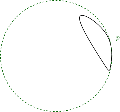
Figure 2: The manifold $\mathcal{M}_{0}$ is $R$-exposed. It is tangent to the dashed sphere at a point $p$ and the corresponding ball contains $\mathcal{M}_{0}.$

Lemma 3.1.

Let $A\subset\mathbb{R}^{n}$ be a closed set, $p\in A$ and $z\in\mathbb{R}^{n}$. Then $p$ is a furthest point from $z$ in $A$ if and only if

$$\langle z-p,q-p\rangle\geq\frac{1}{2}|q-p|^{2}$$ (7)

for all $q\in A$.

Proof.

From the identity

$$|z-q|^{2}=|(z-p)-(q-p)|^{2}=|z-p|^{2}+|q-p|^{2}-2\langle z-p,q-p\rangle$$

one sees that (7) is equivalent to the inequality $|z-q|^{2}\leq|z-p|^{2}$, and the lemma follows. ∎

Lemma 3.2.

A manifold $\mathcal{M}\subset\mathbb{R}^{n}$ is $R$-exposed if and only if for every $p\in\mathcal{M}$ there exists a unit vector $\nu_{p}\in T_{p}^{\perp}\mathcal{M}$ such that

$$\langle q-p,\nu_{p}\rangle\geq\frac{1}{2R}|q-p|^{2}$$ (8)

for all $q\in M$.

Proof.

A point $p\in\mathcal{M}$ is $R$-exposed if and only if there exists $z\in\mathbb{R}^{n}$ (the center of the $R$-ball from the definition) such that $|z-p|=R$ and $p$ is furthest from $z$ in $\mathcal{M}$. For $z=p-R\nu_{p}$, where $\nu_{p}$ is a unit vector, the inequality (7) is equivalent to (8). Differentiating (8) with respect to $q$ at $q=p$ shows that $\nu_{p}\in T_{p}^{\perp}\mathcal{M}$. ∎

3.1 ${\epsilon}$-denseness of the $R$-exposedness condition

Figure 3: Project a flattened version $\mathcal{M}:=\Pi_{H}\mathcal{M}_{0}$ of $\mathcal{M}_{0}$ onto a sphere of large radius. The image $\mathcal{M}_{1}$ of this projection satisfies the $R$-exposedness condition

The condition of $R$-exposedness is ${\epsilon}$-dense in the sense of the following lemma.

Lemma 3.3.

Let $0<{\epsilon}<c.$ Let $\mathcal{M}$ belong to $\mathcal{G}(d,n,V,\tau).$ Then, if $n>\frac{CV}{\omega_{d}}(\min(\frac{\tau}{2d},\frac{{\epsilon}\tau}{2}))^{-d}$, there exists a manifold $\mathcal{M}_{1}\in\mathcal{G}(d,n,V,\tau(1-C{\epsilon}))$ such that the Hausdorff distance $d_{H}(\mathcal{M},\mathcal{M}_{1})<{\epsilon}\tau$ and $\mathcal{M}_{1}$ is $R$-exposed for $R=({\epsilon}\tau)^{-1}.$

Proof.

Let $\mathcal{N}$ be a finite subset of $\mathcal{M}$ of minimum size, such that for all $x\in\mathcal{M}$ there exists $z\in\mathcal{N}$ with $|x-z|<{\epsilon}\tau.$

Claim 3.1.

$|\mathcal{N}|\leq n.$

Proof of Claim 3.1..

The cardinality of a minimum ${\epsilon}^{\prime}$-cover equals is less or equal to the cardinality of a maximal set of disjoint ${\epsilon}^{\prime}/2$-balls (with respect to the Euclidean metric). Let $p\in\mathcal{M}$ and $\mathcal{M}_{p}:=\mathcal{M}\cap B_{\min(\tau/2d,{\epsilon}\tau/2)}^{D}(p)$. Then, by Lemma A.2 for every $q\in\mathcal{M}_{p}$, the projection $\Pi_{q}$ on to the tangent space at $q$ and the projection $\Pi_{p}$ on to the tangent space at $p$ satisfy $\|\Pi_{q}-\Pi_{p}\|<\min(C{\epsilon},Cd^{-1}).$ It follows that the volume of $\mathcal{M}_{p}$ is greater than $c\omega_{d}\min(\frac{\tau}{2d},\frac{{\epsilon}\tau}{2})^{d}.$ Let $\mathcal{N}^{\prime}$ be a maximal disjoint set of $\min(\frac{\tau}{2d},\frac{{\epsilon}\tau}{2})-$balls in $\mathcal{M}$ (with respect to the Euclidean metric). Due to the disjointness of the different $\mathcal{M}_{p}$ when $p$ ranges over $\mathcal{N}^{\prime}$,

$$\sum_{p\in\mathcal{N}^{\prime}}\mathrm{vol}\mathcal{M}_{p}\leq\mathrm{vol}\mathcal{M}.$$

Therefore,

$$|\mathcal{N}|\leq|\mathcal{N}^{\prime}|\leq\frac{CV}{\omega_{d}\min(\frac{\tau}{2d},\frac{{\epsilon}\tau}{2})^{d}}.$$

The claim follows.

∎

Let $H$ be the unique codimension one hyperplane containing $\mathcal{N}.$ Recall that $\mathcal{M}\subseteq B_{1}^{n}(0).$ Let $\tilde{B}_{R}$ denote the unique ball radius $R=({\epsilon}\tau)^{-1},$ that is tangent to $H,$ at the foot of the perpendicular of the origin to $H.$ Every point in $\Pi_{H}\mathcal{M}$ is at a distance of at most $C{\epsilon}\tau$ from $H\cap B_{1}^{n}(0)$. It is also true that every point in $H\cap B_{1}^{n}(0)$ is at a distance of at most $C{\epsilon}\tau$ from $B^{n}_{1}(0)\cap\partial\tilde{B}_{R}.$ Therefore every point in $\mathcal{M}$ is at a distance of at most $C{\epsilon}\tau$ from $B^{n}_{1}(0)\cap\partial\tilde{B}_{R},$ and hence from $\partial\tilde{B}_{R}.$ Let $\Pi_{R}:=\Pi_{\tilde{B}_{R}}$ denote the projection map from $Tub_{\frac{R}{2}}\left(\partial\tilde{B}_{R}\right),$ the tubular neighborhood of $\partial\tilde{B}_{R}$ of radius $\frac{R}{2},$ to $\partial\tilde{B}_{R}$ that maps each point to the nearest point on $\partial\tilde{B}_{R}$. We proceed to prove the following claim.

Claim 3.2.

$\mathcal{M}_{1}:=\Pi_{R}(\Pi_{H}\mathcal{M})$ belongs to $\mathcal{G}(d,n,V,\tau(1-C{\epsilon}))$.

Proof of Claim 3.2.

It follows from Lemma 3.3, page 23 of [45], that

$$\Pi_{H}\mathcal{M}\in\mathcal{G}(d,n,V,\tau(1-C{\epsilon})).$$ (9)

Therefore, in order to prove this claim, it suffices to show that the reach of $\Pi_{H}\mathcal{M}$ does not decrease by more than $C{\epsilon}\tau$ under the application of $\Pi_{R}.$ Let $p$ and $q$ be two points on $\Pi_{H}\mathcal{M}.$ Let $o$ be the center of $\tilde{B}_{R}.$ Let the $d+1$-dimensional subspace containing $Tan(p,\Pi_{H}\mathcal{M})$ and $o$ be $S.$ The sine of the angle between $qo$ and the projection of $qo$ on $S$ is less than $2R^{-1}=2{\epsilon}\tau,$ and the cosine of the angle between $qo$ and any vector in $Tan(p,\Pi_{H}\mathcal{M})$ is less than $C{\epsilon}\tau.$ Similarly, the sine of the angle between $qo$ and a normal to $H$ is less than $2R^{-1}=2{\epsilon}\tau.$ Thus the operator norm $\|\Pi_{1}-\Pi_{2}\|$ where $\Pi_{1}$ is the orthoprojection on to $Tan(p,\Pi_{H}\mathcal{M})$ and $\Pi_{2}$ is the orthoprojection on to $Tan(\Pi_{R}p,\Pi_{R}\Pi_{H}\mathcal{M}),$ is less than $C{\epsilon}\tau.$ Therefore,

$$dist(\Pi_{R}q,Tan(\Pi_{R}p,\Pi_{R}\Pi_{H}\mathcal{M}))\leq(1+C\frac{{\epsilon}\tau}{R})dist(q,Tan(p,\Pi_{H}\mathcal{M})).$$

$\Pi_{R}$ restricted to $H$ is a real analytic diffeomorphism from $H$ to an open hemisphere in $\partial\tilde{B}_{R}$ and a contraction with respect to the usual Euclidean and Riemannian metrics respectively on $H,$ and $\partial\tilde{B}_{R}.$ Together with Proposition 2.1 the claim follows. ∎

Note that $\mathcal{M}_{1}$ is $R$-exposed because $\mathcal{M}_{1}\subseteq\partial\tilde{B}_{R}.$ ∎

3.2 Derivative estimates

Lemma 3.4.

Let $\mathcal{M}\subset\mathbb{R}^{n}$ be a closed $C^{2,1}-$submanifold with $\mathrm{reach}(\mathcal{M})\geq\tau$. Fix $p\in\mathcal{M}$ and define open sets $U\subset T_{p}\mathcal{M}$ and $Q\subset\mathbb{R}^{n}$ by

$$U=\{x\in T_{p}\mathcal{M}:|x|<\tfrac{\tau}{8}\}$$

and

$$Q=\{x\in\mathbb{R}^{n}:|\Pi_{T_{p}\mathcal{M}}(x)|<\tfrac{\tau}{8}\text{ and }|\Pi_{T^{\perp}_{p}\mathcal{M}}(x)|<\tfrac{\tau}{8}\}.$$

Then the set $(\mathcal{M}-p)\cap Q$ is a graph of a $C^{2,1}$ function

$$f\colon U\to T_{p}^{\perp}\mathcal{M}$$

such that the following estimates hold for all $x\in U$ and some absolute constant $C>0$:

$$|f(x)| \leq\tau^{-1}|x|^{2},$$ (10)

$$\|d_{x}f\| \leq C\tau^{-1}|x|,$$ (11)

$$\|d^{2}_{x}f\| \leq C\tau^{-1}$$ (12)

where $d_{x}f$ and $d^{2}_{x}f$ are the first and second differentials of $f$ at $x$, and $\|d_{x}f\|$ and $\|d^{2}_{x}f\|$ are their operator norms.

If, in addition, the second fundamental form of $\mathcal{M}$ is $\Lambda$-Lipschitz with $\Lambda\geq\tau^{-2}$, then the map $x\mapsto d_{x}^{2}f$ is $C\Lambda$-Lipschitz:

$$\|d^{2}_{x}f-d^{2}_{y}f\|\leq C\Lambda|x-y|$$ (13)

for all $x,y\in U$.

Proof.

The existence of $f$ and the estimates (10), (11), (12) follow from [45, Lemma A.2]. It remains to prove (13). Throughout the proof we use the short notation $\Pi_{q}=\Pi_{T_{q}\mathcal{M}}$ and $\Pi_{q}^{\perp}=\Pi_{T_{q}^{\perp}\mathcal{M}}$ for the orthogonal projections to the tangent and normal spaces at $q\in\mathcal{M}$. All absolute constants are denoted by the same letter $C$.

Consider the local parametrization $\varphi$ of $\mathcal{M}$ determined by $f$, that is $\varphi\colon U\to\mathbb{R}^{n}$ is a map given by

$$\varphi(x)=x+f(x),\qquad x\in U.$$

For every $x\in U$, the parametrization and the second fundamental form of $\mathcal{M}$ at $\varphi(x)$ are related by the formula

$$\mathcal{S}_{\varphi(x)}(d_{x}\varphi(v),d_{x}\varphi(w)))=\Pi_{\varphi(x)}^{\perp}(d_{x}^{2}\varphi(v,w))=\Pi_{\varphi(x)}^{\perp}(d_{x}^{2}f(v,w))$$ (14)

for all $v,w\in T_{p}\mathcal{M}$. This formula defines $\mathcal{S}_{\varphi(x)}$ on the tangent space. By our convention, $\mathcal{S}_{\varphi(x)}$ is extended to the whole $\mathbb{R}^{n}$ via projection:

$$\mathcal{S}_{\varphi(x)}(\xi,\eta)=\mathcal{S}_{\varphi(x)}(\Pi_{\varphi(x)}(\xi),\Pi_{\varphi(x)}(\eta))$$

for all $\xi,\eta\in\mathbb{R}^{n}$. These identities imply that $\|\mathcal{S}_{\varphi(x)}\|\leq C\tau^{-1}$ for all $x\in U$.

Fix $x,y\in U$ sufficiently close to each other and a unit vector $v\in T_{p}M$. Let $\delta=|x-y|$, $v_{x}=d_{x}\varphi(v)$ and $v_{y}=d_{y}\varphi(v)$. By (11) and (12) we have $|v_{x}|\leq C$, $|v_{y}|\leq C$,

$$\|d_{x}f-d_{y}f\|\leq C\tau^{-1}\delta$$ (15)

and hence $|v_{x}-v_{y}|\leq C\tau^{-1}\delta$. By the $\Lambda$-Lipschitz continuity of the second fundamental form,

$$|\mathcal{S}_{\varphi(x)}(v_{x},v_{x})-\mathcal{S}_{\varphi(y)}(v_{x},v_{x})|\leq\Lambda\cdot|\varphi(x)-\varphi(y)|\cdot|v_{x}|^{2}\leq C\Lambda\delta.$$

From the above bounds on $\|\mathcal{S}\|$, $|v_{x}|$, $|v_{y}|$, $|v_{x}-v_{y}|$, one sees that

$$|\mathcal{S}_{\varphi(y)}(v_{x},v_{x})-\mathcal{S}_{\varphi(y)}(v_{y},v_{y})|\leq C\|\mathcal{S}_{\varphi(y)}\|\cdot|v_{x}|\cdot|v_{x}-v_{y}|\leq C\tau^{-2}\delta\leq C\Lambda\delta$$

where the last inequality follows from the assumption $\Lambda\geq\tau^{-2}$. Thus

$$|\mathcal{S}_{\varphi(x)}(v_{x},v_{x})-\mathcal{S}_{\varphi(y)}(v_{y},v_{y})|\leq C\Lambda\delta.$$

By (14) this is equivalent to

$$|\Pi_{\varphi(x)}^{\perp}(d_{x}^{2}f(v,v))-\Pi_{\varphi(y)}^{\perp}(d_{y}^{2}f(v,v))|\leq C\Lambda\delta.$$ (16)

The estimate (15) implies a bound for the distance between the tangent planes $T_{\varphi(x)}\mathcal{M}$ and $T_{\varphi(y)}\mathcal{M}$ (see (22)):

$$\|\Pi_{\varphi(y)}^{\perp}-\Pi_{\varphi(x)}^{\perp}\|=\|\Pi_{\varphi(y)}-\Pi_{\varphi(x)}\|\leq C\tau^{-1}\delta,$$

therefore

$$|\Pi_{\varphi(y)}^{\perp}(d_{y}^{2}f(v,v))-\Pi_{\varphi(x)}^{\perp}(d_{y}^{2}f(v,v))|\leq C\tau^{-1}\delta\|d_{y}^{2}f\|\leq C\tau^{-2}\delta\leq C\Lambda\delta.$$

By (16) it follows that

$$\left|\Pi_{\varphi(x)}^{\perp}\big{(}d_{x}^{2}f(v,v)-d_{y}^{2}f(v,v)\big{)}\right|\leq C\Lambda\delta.$$ (17)

Let $P\colon T_{p}^{\perp}\mathcal{M}\to T_{\varphi(x)}^{\perp}\mathcal{M}$ be the restriction of $\Pi_{\varphi(x)}^{\perp}$ to $T_{p}^{\perp}\mathcal{M}$. Since $\Pi_{\varphi(x)}$ is the graph of the linear map $d_{x}f\colon T_{p}\mathcal{M}\to T_{p}^{\perp}\mathcal{M}$ satisfying $\|d_{x}f\|\leq C\tau^{-1}|x|\leq C$ (see (11)), $P$ is bijective and $\|P^{-1}\|\leq C$. This and (17) imply that

$$|d_{x}^{2}f(v,v)-d_{y}^{2}f(v,v)|=\left|P^{-1}\circ\Pi_{\varphi(x)}^{\perp}\big{(}d_{x}^{2}f(v,v)-d_{y}^{2}f(v,v)\big{)}\right|\leq C\Lambda\delta$$

and (12) follows. ∎

Lemma 3.5.

Let $f$ be as in Lemma 3.4. Then for all $x,y\in T_{p}\mathcal{M}$ such that $\max\{|x|,|y|\}\leq\frac{1}{4}\tau$,

$$|f(x+y)-f(y)-d_{y}f(x)-f(x)|\leq C\Lambda|x|^{2}|y|.$$

Proof.

Define $h\colon[0,1]\to T_{p}^{\perp}\mathcal{M}$ by

$$h(t)=f(tx+y)-f(y)-td_{y}f(x)-f(tx).$$

We have $h(0)=0$, $h^{\prime}(0)=0$ and

$$|h^{\prime\prime}(t)|=|d^{2}_{tx+y}f(x,x)-d^{2}_{tx}f(x,x)|\leq C\Lambda|x|^{2}|y|$$

from the Lipschitz condition on $d^{2}f$. Hence $|h(1)|\leq C\Lambda|x|^{2}|y|$ as claimed. ∎

4 Geometric bounds preserved under projection

4.1 Preservation of uniform exposedness by projection

Here we need the $\Lambda$-Lipschitz continuity of the second fundamental form. We assume below that

$$\Lambda\geq\tau^{-2}$$ (18)

where $\tau$ is the reach bound, otherwise $\Lambda$ should be replaced by $\max\{\Lambda,\tau^{-2}\}$ in some formulas.

We will need the following well-known facts about distances between linear subspaces: When $X,Y\subset\mathbb{R}^{n}$ are linear subspaces with $\dim X=\dim Y$, we define analogously to [55], Chapter IV, section 2.1,

$$\delta(X,Y) =\sup\{dist(x,Y):x\in X\cap B_{1}^{n}\}$$ (19)

$$=\sup\{dist(x,Y\cap B_{1}^{n}):x\in X\cap B_{1}^{n}\},$$

and $B_{1}^{n}$ is the unit ball in $\mathbb{R}^{n}$ centered at 0. Note that it always holds that $0\leq\delta(X,Y)\leq 1$.

If $\delta(X,Y)<1$ then [56, Lemma 221] implies that either $\delta(Y,X)=\delta(X,Y)$ or $Y$ has a proper subspace $Y_{0}$ that is isomorphic to $X$. As $\dim X=\dim Y$, the latter is not possible and hence $\delta(X,Y)<1$ implies that $\delta(Y,X)=\delta(X,Y)<1$. By changing roles of $X$ and $Y$ we see that $\delta(Y,X)<1$ implies that $\delta(X,Y)=\delta(Y,X)<1$. Thus we see that either both $\delta(X,Y)$ and $\delta(Y,X)$ are equal to $1$, or both $\delta(X,Y)$ and $\delta(Y,X)$ are strictly less than 1 and $\delta(X,Y)=\delta(Y,X)$. These arguments show that in all possible cases

$$\delta(X,Y)=\delta(Y,X).$$ (20)

We observe that

$$\hat{\delta}(X,Y):=\max(\delta(X,Y),\delta(X,Y))=d_{H}(X\cap B_{1}^{n},Y\cap\mathcal{B}_{1}^{n}).$$

In the case when $\delta(X,Y)=\delta(Y,X)=1$, there is there is non-zero vector $x\in X\cap Y^{\perp}$ and we see that $\|\Pi_{X}-\Pi_{Y}\|=\hat{\delta}(X,Y)=1$. On the other hand, when $\hat{\delta}(X,Y)<1$, [55, Theorem I-6.34], and [55, Lemma 221] imply that

$$\|\Pi_{X}-\Pi_{Y}\|=\|(I-\Pi_{X})\Pi_{Y}\|=\|(I-\Pi_{Y})\Pi_{X}\|=\hat{\delta}(X,Y).$$ (21)

In particular, this implies that

$$\hat{\delta}(X,Y)=\|\Pi_{X}-\Pi_{Y}\|=\|\Pi_{X^{\perp}}-\Pi_{Y^{\perp}}\|=\hat{\delta}(X^{\perp},Y^{\perp}).$$ (22)

Lemma 4.1.

Let $\mathcal{M}\subset\mathbb{R}^{n}$ be a manifold with $\mathrm{reach}(\mathcal{M})\geq\tau$ and $S\subset\mathbb{R}^{n}$ a linear subspace such that

$$\sup_{x\in\mathcal{M}}dist(x,S)\leq\alpha^{2}\tau$$

for some $\alpha\in(0,\frac{1}{4})$. Then for every $p\in\mathcal{M}$ and every unit vector $v\in T_{p}\mathcal{M}$,

$$dist(v,S)=|\Pi_{S^{\perp}}(v)|\leq 3\alpha.$$

Proof.

Let $p\in\mathcal{M}$ and let $v\in T_{p}\mathcal{M}$ be unit vector. We borrow from [45] the following fact (see [45, Lemma A.1]): the set $\Pi_{T_{p}\mathcal{M}}(\mathcal{M}\cap B_{\tau}(p))$ contains the ball of radius $\frac{\tau}{4}$ in $T_{p}\mathcal{M}$ centered at $\Pi_{T_{p}\mathcal{M}}(p)$. Hence there exists $q\in\mathcal{M}$ such that $|q-p|<\tau$ and $\Pi_{T_{p}\mathcal{M}}(q-p)=\alpha\tau v$. Then

$$q-p=\alpha\tau v+w$$

for some $w\in T_{p}^{\perp}\mathcal{M}$. Since both $p$ and $q$ lie within distance $\alpha^{2}\tau$ from $S$,

$$|\Pi_{S^{\perp}}(q-p)|\leq 2\alpha^{2}\tau.$$

By Corollary 2.2 we have $|w|\leq\tau^{-1}|\alpha\tau v|^{2}=\alpha^{2}\tau$, thus

$$|\Pi_{S^{\perp}}(\alpha\tau v)|=|\Pi_{S^{\perp}}(q-p-w)|\leq|\Pi_{S^{\perp}}(q-p)|+|w|\leq 3\alpha^{2}\tau.$$

The claim of the lemma follows by homogeneity. ∎

Lemma 4.2.

There exists an absolute constant $c>0$ such that the following holds. Assume that $\mathcal{M}\subset\mathbb{R}^{n}$ has $\mathrm{reach}(\mathcal{M})\geq\tau$, is $R$-exposed, and has a $\Lambda$-Lipschitz second fundamental form where $\Lambda\geq\tau^{-2}$. Let $S\subset\mathbb{R}^{n}$ be a linear subspace such that

$$\sup_{x\in\mathcal{M}}dist(x,S)<c\,\Lambda^{-2}R^{-4}\tau.$$ (23)

Then $\Pi_{S}(\mathcal{M})$ is $2R$-exposed.

Proof.

We define

$$h=\sup_{x\in\mathcal{M}}dist(x,S)$$

and assume that $h$ is sufficiently small. The required bounds for $h$ will be accumulated in the course of the proof.

Fix $p\in\mathcal{M}$ and define $Y=\Pi_{S}(T_{p}\mathcal{M})$. First we assume that

$$h\leq\alpha^{2}\tau$$ (24)

where $\alpha\in(0,\frac{1}{4})$ is to be chosen later. Lemma 4.1 implies that

$$dist(x,Y)=|\Pi_{Y^{\perp}}(x)|\leq 3\alpha|x|\qquad\text{for all $x\in T_{p}\mathcal{M}$}.$$ (25)

Since $3\alpha<1$, it follows that $\Pi_{S}|_{T_{p}\mathcal{M}}$ is injective and hence $Y$ is a $d$-dimensional linear subspace. It is easy to see that (25) implies a similar property for the orthogonal complements:

$$dist(z,Y^{\perp})=|\Pi_{Y}(z)|\leq 3\alpha|z|\qquad\text{for all $z\in T_{p}^{\perp}\mathcal{M}$}.$$ (26)

We represent $\mathcal{M}-p$ near $0$ as a graph of a function $f\colon U\to T_{p}^{\perp}\mathcal{M}$ where $U$ is the ball of radius $\tau/4$ in $T_{p}\mathcal{M}$ centered at 0, see Lemma 3.4. This defines a local parametrization of $\mathcal{M}$ given by

$$U\ni x\mapsto\varphi(x):=p+x+f(x)$$

We proceed in several steps.

Step 1. We assume that

$$h\leq\Lambda r^{3}$$ (27)

where $r\in(0,\frac{\tau}{4})$ is to be chosen later. We are going to estimate the distance from $f(x)$ to $S$ for $x\in U$ such that $\|x\|\leq r$.

Since $f(0)=0$ and $d_{0}f=0$, we have the Taylor expansion

$$f(x)=\frac{1}{2}d^{2}_{0}f(x,x)+\theta(x).$$ (28)

and an estimate

$$|\theta(x)|\leq C_{1}\Lambda|x|^{3}$$ (29)

where $C_{1}>0$ is an absolute constant such that $d^{2}f$ is $(6C_{1}\Lambda)$-Lipschitz, see Lemma 3.4 (13).

Since $\mathcal{M}$ is contained in the $h$-neighborhood of $S$ and $p\in\mathcal{M}$, we have

$$|\Pi_{S^{\perp}}(x+f(x))|=|\Pi_{S^{\perp}}(\varphi(x)-p)|\leq 2h.$$

Applying this to $x$ and $-x$ and summing the two inequalities we obtain

$$|\Pi_{S^{\perp}}(f(x)+f(-x))|\leq|\Pi_{S^{\perp}}(x+f(x))|+|\Pi_{S^{\perp}}(-x+f(-x))|\leq 4h.$$

By (28) this can be rewritten as

$$|\Pi_{S^{\perp}}(d^{2}_{0}f(x,x)+\theta(x)+\theta(-x))|\leq 4h,$$

therefore, by (29),

$$|\Pi_{S^{\perp}}(d^{2}_{0}f(x,x))|\leq 4h+2C_{1}\Lambda|x|^{3}$$

for all $x\in U$. Substitute $x=rv$ where $v\in T_{p}\mathcal{M}$ is a unit vector, and divide by $r^{2}$. This yields

$$|\Pi_{S^{\perp}}(d^{2}_{0}f(v,v))|\leq 4hr^{-2}+2C_{1}\Lambda r\leq(2C_{1}+4)\Lambda r$$

by (27). This holds for all unit vectors $v\in T_{p}\mathcal{M}$, therefore, by homogeneity,

$$|\Pi_{S^{\perp}}(d^{2}_{0}f(x,x))|\leq(2C_{1}+4)\Lambda r|x|^{2}$$ (30)

for all $x\in T_{p}\mathcal{M}$. If $|x|\leq r$ then (29) implies that $|\theta(x)|\leq C_{1}\Lambda r|x|^{2}$, hence by (28) and (30),

$$|\Pi_{S^{\perp}}(f(x))|\leq(3C_{1}+4)\Lambda r|x|^{2}=:C_{2}\Lambda r|x|^{2}$$ (31)

for all $x\in U$ such that $|x|\leq r$.

Step 2. Let $\nu_{p}\in T_{p}^{\perp}\mathcal{M}$ be a unit vector from Lemma 3.2. Define $w_{p}=\Pi_{Y^{\perp}}(\nu_{p})$. Our plan is to show that

$$\langle\Pi_{S}(q-p),w_{p}\rangle\geq\frac{1}{4R}|\Pi_{S}(q-p)|^{2}.$$ (32)

and then apply Lemma 3.2 to $\Pi_{S}(\mathcal{M})$ with $\frac{w_{p}}{|w_{p}|}$ in place of $\nu_{p}$.

In this step we handle the case when $|q-p|\leq r$ where $r$ is the same as in Step 1. In this case $q=\varphi(x)=p+x+f(x)$ for some $x\in U$ such that $|x|\leq r$, and

$$\langle\Pi_{S}(q-p),w_{p}\rangle=\langle\Pi_{S}(x)+\Pi_{S}(f(x)),w_{p}\rangle=\langle\Pi_{S}(f(x)),w_{p}\rangle$$ (33)

since $\Pi_{S}(x)\in Y$ and $w_{p}\in Y^{\perp}$. We rewrite the right-hand side as

$$\langle\Pi_{S}(f(x)),w_{p}\rangle=\langle f(x)-\Pi_{S^{\perp}}(f(x)),\nu_{p}-\Pi_{Y}(\nu_{p})\rangle=A_{0}-A_{1}-A_{2}+A_{3}$$

where

$$A_{0} =\langle f(x),\nu_{p}\rangle,$$

$$A_{1} =\langle\Pi_{S^{\perp}}(f(x)),\nu_{p}\rangle,$$

$$A_{2} =\langle f(x),\Pi_{Y}(\nu_{p})\rangle.$$

and $A_{3}=\langle\Pi_{S^{\perp}}(f(x)),\Pi_{Y}(\nu_{p})\rangle=0$ since $Y\subset S$. Thus

$$\langle\Pi_{S}(q-p),w_{p}\rangle=A_{0}-A_{1}-A_{2}.$$ (34)

We are going to estimate $A_{0}$ from below and $A_{1},A_{2}$ from above.

Since $x\in T_{p}\mathcal{M}$ and $\nu_{p}\in T_{p}^{\perp}\mathcal{M}$, we have

$$A_{0}=\langle f(x),\nu_{p}\rangle=\langle x+f(x),\nu_{p}\rangle=\langle q-p,\nu_{p}\rangle\geq\frac{1}{2R}|q-p|^{2}$$ (35)

by Lemma 3.2. For $A_{1}$ we have

$$A_{1}=\langle\Pi_{S^{\perp}}(f(x)),\nu_{p}\rangle\leq|\Pi_{S^{\perp}}(f(x))|\leq C_{2}\Lambda r|x|^{2}$$

by (31). We assume that $r$ is chosen so small that

$$C_{2}\Lambda r\leq\frac{1}{8R},$$ (36)

then the previous inequality implies that

$$A_{1}\leq\frac{1}{8R}|x|^{2}\leq\frac{1}{8R}|q-p|^{2}.$$ (37)

For $A_{2}$ we have

$$A_{2}=\langle f(x),\Pi_{Y}(\nu_{p})\rangle=\langle\Pi_{Y}(f(x)),\Pi_{Y}(\nu_{p})\rangle\leq|\Pi_{Y}(f(x))|\cdot|\Pi_{Y}(\nu_{p})|.$$

Since $f(x)$ and $\nu_{p}$ belong to $T_{p}^{\perp}\mathcal{M}$, (26) implies that

$$|\Pi_{Y}(f(x))|\leq 3\alpha|f(x)|$$

and

$$|\Pi_{Y}(\nu_{p})|\leq 3\alpha|\nu_{p}|=3\alpha,$$ (38)

therefore

$$A_{2}\leq 9\alpha^{2}|f(x)|\leq 9\alpha^{2}\tau^{-1}|x|^{2}$$

where the last inequality follows from (10). We now assume that $\alpha$ is so small that

$$9\alpha^{2}\tau^{-1}\leq\frac{1}{8R},$$ (39)

then the previous inequality implies that

$$A_{2}\leq\frac{1}{8R}|x|^{2}\leq\frac{1}{8R}|q-p|^{2}.$$ (40)

Now (34) and the estimates (35), (37), (40) imply that

$$\langle\Pi_{S}(q-p),w_{p}\rangle\geq\frac{1}{4R}|q-p|^{2}\geq|\Pi_{S}(q-p)|^{2}$$

Thus (32) holds for all $q\in\mathcal{M}$ such that $|p-q|\leq r$.

Step 3. Now we prove (32) for points $q\in\mathcal{M}$ such that $|q-p|\geq r$. Recall that

$$\langle q-p,\nu_{p}\rangle\geq\frac{1}{2R}|q-p|^{2}.$$

by Lemma 3.2. Since $p$ and $q$ belong to the $h$-neighborhood of $S$, we have $|\Pi_{S^{\perp}}(q-p)|\leq 2h$, hence

$$\langle\Pi_{S^{\perp}}(q-p),\nu_{p}\rangle\leq 2h\leq 2\Lambda r^{3}\leq\frac{1}{8R}r^{2}\leq\frac{1}{8R}|q-p|^{2}$$

by (27), (36) and the fact that $C_{2}\geq 4$, see (30). Subtracting this from the previous inequality we obtain

$$\langle\Pi_{S}(q-p),\nu_{p}\rangle=\langle q-p,\nu_{p}\rangle-\langle\Pi_{S^{\perp}}(q-p),\nu_{p}\rangle\geq\frac{3}{8R}|q-p|^{2}.$$ (41)

Now we estimate $\langle\Pi_{S}(q-p),w_{p}-\nu_{p}\rangle$. Since $w_{p}-\nu_{p}=\Pi_{Y}(\nu_{p})$,

$$|\langle\Pi_{S}(q-p),w_{p}-\nu_{p}\rangle|\leq|\Pi_{S}(q-p)|\cdot|\Pi_{Y}(\nu_{p})|\leq 3\alpha|q-p|$$ (42)

by (38). We now assume that

$$\alpha\leq\frac{r}{16R},$$ (43)

then the previous inequality implies that

$$|\langle\Pi_{S}(q-p),w_{p}-\nu_{p}\rangle|\leq\frac{r}{8R}|q-p|\leq\frac{1}{8R}|q-p|^{2}$$

due to the assumption $|q-p|\geq r$. Subtracting this from (41) we obtain

$$\langle\Pi_{S}(q-p),w_{p}\rangle=\langle\Pi_{S}(q-p),\nu_{p}\rangle+\langle\Pi_{S}(q-p),w_{p}-\nu_{p}\rangle\geq\frac{1}{4R}|q-p|^{2}.$$

Thus (32) holds if $|q-p|\geq r$.

Step 4. In the previous steps we have shown that (32) holds for all $q\in\mathcal{M}$. Since $|w_{p}|\leq 1$, it follows that the vector $w_{p}^{\prime}=\frac{w_{p}}{|w_{p}|}$ satisfies

$$\langle\Pi_{S}(q)-\Pi_{S}(p),w_{p}^{\prime}\rangle\geq\frac{1}{4R}|q-p|^{2}\geq\frac{1}{4R}|\Pi_{S}(q)-\Pi_{S}(p)|^{2}$$

for all $q\in\mathcal{M}$. By Lemma 3.2 applied to $\Pi_{S}(\mathcal{M})$ and $w_{p}^{\prime}$ in place of $\nu_{p}$ this implies that $\Pi_{S}(\mathcal{M})$ is $2R$-exposed.

Now we collect the assumptions made in the course of the argument. Those are bounds (24) and (27) on $h$, (39) and (43) on $\alpha\in(0,\frac{1}{4})$, and (36) on $r\in(0,\frac{\tau}{4})$. Taking into account the assumption $\Lambda\geq\tau^{-2}$ and the obvious inequality $R\geq\tau$, one sees that the required bounds are satisfied by setting $r=c_{1}\Lambda^{-1}R^{-1}$, $\alpha=c_{2}\Lambda^{-1}R^{-2}$s and assuming that $h<c\Lambda^{-2}R^{-4}\tau$, where $c_{1},c_{2},c>0$ are suitable absolute constants. This finishes the proof of Lemma 4.2. ∎

5 Principal Component Analysis and dimension reduction

We take an adequate number of random samples, and perform Principal Component Analysis, and project the data on to a subspace $S$ of dimension $D$, as described in [45]. With high probability, the image manifold $\mathcal{M}$ has a Hausdorff distance of less than $c{\epsilon}$ from the original manifold $\mathcal{M}_{0}.$ Let $K$ be the convex hull of $\mathcal{M}.$

Let $S$ be an affine subspace of $\mathbb{R}^{n}$. Let $\Pi_{S}$ denote orthogonal projection onto $S$. Let the span of the first $d$ canonical basis vectors be denoted $\mathbb{R}^{d}$ and the span of the last $n-d$ canonical basis vectors be denoted $\mathbb{R}^{n-d}$. Let $\omega_{d}$ be the $d$ dimensional Lebesgue measure of the unit Euclidean ball in $\mathbb{R}^{d}$. Given $\alpha\in(0,1),$ let

$$\beta:=\beta(\alpha)=\sqrt{\frac{1}{10}\left(\frac{\alpha^{2}\tau}{2}\right)^{2}\left(\frac{\alpha^{2}\tau}{4}\right)^{d}\left(\frac{\omega_{d}}{V}\right)}.$$ (44)

Let

$$D:=\left\lfloor\frac{V}{\omega_{d}\beta^{d}}\right\rfloor+1.$$ (45)

Let

$${\epsilon}<\beta^{2}/2.$$ (46)

Below,

$$\delta<\eta/2$$ (47)

will be a small parameter that gives a bound on the probability that the conclusion $\sup_{x\in\mathcal{M}}dist(x,S)<\alpha^{2}\tau$ in Proposition 5.1 fails. Choose

$$N_{D}=\lfloor C(n\sigma^{2}+\sigma^{2}\log(Cn\sigma^{2}/({\epsilon}{\mathbf{\delta}})))\sqrt{\log(C/{\mathbf{\delta}})}(D/{\epsilon}^{2})\rfloor,$$ (48)

where $C$ is a sufficiently large universal constant.

Proposition 5.1 (Proposition 3.1 [45]).

Given $N_{D}$ data points $\{x_{1},\dots,x_{N_{D}}\}$ drawn i.i.d from $\tilde{\mu}$, let $S$ be a $D$ dimensional affine subspace that minimizes

$$\sum_{i=1}^{N_{D}}dist(x_{i},\tilde{S})^{2},$$ (49)

subject to the condition that $\tilde{S}$ is an affine subspace of dimension $D$, and $\beta<c\tau$, where $\beta$ is given by (44).

Then,

$$\mathbb{P}[\sup_{x\in\mathcal{M}}dist(x,S)<\alpha^{2}\tau]>1-\delta.$$ (50)

Recall from Subsection 1.2 that $\mathcal{M}_{0}$ is a $d$-dimensional $C^{2,1}$ submanifold of $\mathbb{R}^{n}$. Let $K_{0}$ be the convex hull of $\mathcal{M}_{0}$. We assume that

$$\mathcal{M}_{0}\subseteq\partial K_{0}\subseteq B^{n}_{1}(0).$$

We also suppose that $\mathcal{M}_{0}$ has volume ($d$-dimensional Hausdorff measure) less or equal to $V$, reach (i.e. normal injectivity radius) greater or equal to $\tau$.

Definition 5.1.

After a suitable orthogonal change of coordinates, we identify $S$ with $\mathbb{R}^{D}$.

1. Let $\mathcal{M}:=\Pi_{S}\mathcal{M}_{0}$.

2. Let $K$ be the convex hull of $\mathcal{M}$.

6 Continuity of outward normal cones

Theorem 6.1.

Let $\mathcal{M}=\mathcal{M}^{d}\subset\mathbb{R}^{n}$ be closed a $C^{2,1}$ submanifold satisfying the above geometric bounds, and let $K=\operatorname{conv}(\mathcal{M})$. Then the outer normal cone $N_{K}(x)$ is a Lipschitz function of $x\in\mathcal{M}$:

$$d_{CH}(N_{K}(x),N_{K}(y))\leq L\|x-y\|$$

for all $x,y\in\mathcal{M}$, where $L>0$ is determined by the parameters $R,\tau,\Lambda$ from the geometric bounds. In fact, $CR(\Lambda+\tau^{-2})$.

Proof.

The next two lemmas are from convex geometry. The first one allows us to estimate the distances between tangent cones instead of outer normal cones, using the fact that $N_{K}(p)=T_{K}(p)^{\circ}$.

Lemma 6.2.

For any closed convex cones $K_{1},K_{2}\subset\mathbb{R}^{n}$,

$$d_{CH}(K_{1}^{\circ},K_{2}^{\circ})=d_{CH}(K_{1},K_{2}).$$

Proof.

Denote $s=d_{CH}(K_{1},K_{2})$; we may assume that $s>0$. W.l.o.g. the distance $s$ is realized by points $x_{0}\in K_{1}\cap B_{1}(0)$ and $y_{0}\in K_{2}\cap B_{1}(0)$ such that $y_{0}$ is a nearest point to $x_{0}$ in $K_{2}\cap B_{1}(0)$ and $\|x_{0}-y_{0}\|=s$. Since $K_{1}$ and $K_{2}$ are cones, we have $\|x_{0}\|=1$. Define $v=\frac{x_{0}-y_{0}}{\|x_{0}-y_{0}\|}=\frac{x_{0}-y_{0}}{s}$.

Observe that $y_{0}$ is a nearest point to $x_{0}$ in the whole cone $K_{2}$. This implies that $\langle x_{0}-y_{0},y_{0}\rangle=0$. Therefore

$$\langle x_{0}-y_{0},x_{0}\rangle=\langle x_{0}-y_{0},x_{0}-y_{0}\rangle=s^{2}$$

and

$$\langle v,x_{0}\rangle=s.$$

Since $y_{0}$ is nearest to $x_{0}$ in $K_{2}$ and $K$ is convex, for every $y\in K_{2}$ we have

$$\langle y,x_{0}-y_{0}\rangle=\langle y-y_{0},x_{0}-y_{0}\rangle\leq 0.$$

Therefore $v\in K_{2}^{\circ}$. Consider an arbitrary $w\in K_{1}^{\circ}$ and estimate $\|v-w\|$ from below as follows: First observe that $\langle w,x_{0}\rangle\leq 0$ since $x_{0}\in K_{1}$ and $w\in K_{1}^{\circ}$. Then

$$\|v-w\|\geq\langle v-w,x_{0}\rangle=\langle v,x_{0}\rangle-\langle w,x_{0}\rangle\geq s$$

since $\langle v,x_{0}\rangle=s$ and $\langle w,x_{0}\rangle\leq 0$. (The last inequality follows from the facts that $x_{0}\in K_{1}$ and $w\in K_{1}^{\circ}$).

Thus $\|v-w\|\geq s$ for all $w\in K_{1}^{\circ}$. Since $v\in K_{1}^{\circ}$ and $\|v\|=1$, this implies that

$$d_{CH}(K_{1}^{\circ},K_{2}^{\circ})\geq s=d_{CH}(K_{1},K_{2}).$$

The reverse inequality follows from the same arguments applied to $K_{1}^{\circ}$ and $K_{2}^{\circ}$ in place of $K_{1}$ and $K_{2}$, and the Bipolar Theorem. ∎

The next lemma estimates the distance between convex cones generated by subsets of $\mathbb{R}^{n}$. To get a sensible estimate we have to assume that each set is strictly separated away from 0 by some hyperplane, this is controlled by the parameter $\alpha.$

Lemma 6.3.

Let $\alpha,\delta>0$ and let $X_{1},X_{2}\subset\mathbb{R}^{n}$ be such that

1. There exist unit vectors $v_{1},v_{2}\in\mathbb{R}^{n}$ such that $\langle x,v_{i}\rangle\geq\alpha$ for all $x\in X_{i}$, $i=1,2$.

2. For every $x\in X_{1}$ there exists $y\in\operatorname{cone}(X_{2})$ such that $\|x-y\|\leq\delta$, and the same holds with $X_{1}$ and $X_{2}$ interchanged.

Then

$$d_{CH}(\operatorname{conv}\operatorname{cone}(X_{1}),\operatorname{conv}\operatorname{cone}(X_{2}))\leq\alpha^{-1}\delta.$$

Proof.

Let $Y_{i}=\operatorname{conv}(X_{i})$, $i=1,2$. It is easy to see that both assumptions are preserved if $X_{i}$ is replaced by $Y_{i}$, $i=1,2$. The first assumption implies that $\|x\|\geq\alpha$ for all $x\in Y_{1}\cup Y_{2}$. Note that $\operatorname{conv}\operatorname{cone}(X_{i})=\operatorname{cone}(Y_{i})$.

Every point from $\operatorname{cone}(Y_{1})\cap B_{1}(0)$ can be written as $sx$ for some $x\in Y_{1}$ and $s\in[0,\alpha^{-1}]$. By assumptions there exists $y\in\operatorname{cone}(Y_{2})$ such that $\|x-y\|\leq\delta$. Moreover $y$ can be chosen so that $\|y\|\leq\|x\|$ (replace $y$ by the point nearest to $x$ on the ray $\{ty:y\geq 0\}$). Then $\|sy\|\leq\|sx\|\leq 1$.

Now for any point $sx\in\operatorname{cone}(Y_{1})\cap B_{1}(0)$, where $x\in Y_{1}$ and $s\in[0,\alpha^{-1}]$, we have a point $sy\in\operatorname{cone}(Y_{2})\cap B_{1}(0)$ with $\|sx-sy\|=s\|x-y\|\leq\alpha^{-1}\delta$. The same holds with indices 1 and 2 exchanged, hence the desired inequality holds. ∎

Fix $p\in\mathcal{M}$ and let $K=\operatorname{conv}(\mathcal{M})$. We are interested in the tangent cone

$$T_{K}(p)=\operatorname{cl}\operatorname{conv}\operatorname{cone}(\mathcal{M}-p).$$

In order to be able to apply Lemma 6.3, we split off a linear part $T_{p}\mathcal{M}$ of this cone. Namely let $\Pi_{p}^{\perp}$ denote the orthogonal projection from $\mathbb{R}^{n}$ to $T_{p}^{\perp}\mathcal{M}$, then

$$T_{K}(p)=T_{p}\mathcal{M}+T_{K}^{\perp}(p).$$

where

$$T_{K}^{\perp}(p)=T_{K}(p)\cap T_{p}^{\perp}\mathcal{M}=\operatorname{cl}\operatorname{conv}\operatorname{cone}(\Pi_{p}^{\perp}(\mathcal{M}-p)).$$ (51)

Now with Lemma 6.2 it suffices to prove that $T_{K}^{\perp}(p)$ is a Lipschitz function of $p$ (since $T_{p}\mathcal{M}$ is a Lipschitz function of $p$ with Lipschitz constant $\tau^{-1}$).

Define a map $\Phi_{p}\colon\mathcal{M}\setminus\{p\}\to T_{p}^{\perp}\mathcal{M}$ by

$$\Phi_{p}(x)=\frac{\Pi_{p}^{\perp}(x-p)}{\|x-p\|^{2}}$$

and let $X_{p}$ be the image of $\Phi_{p}$:

$$X_{p}=\{\Phi_{p}(x)\mid x\in\mathcal{M}\setminus\{p\}\}.$$

From (51) we have

$$T_{K}^{\perp}(p)=\operatorname{cl}\operatorname{conv}\operatorname{cone}(X_{p})$$ (52)

Let $\nu_{p}\in T_{p}^{\perp}\mathcal{M}$ be a unit vector from Lemma 3.2, then

$$\langle\Phi_{p}(x),\nu_{p}\rangle=\|x-p\|^{-2}\langle x-p,\nu_{p}\rangle\geq\frac{1}{2R}$$

for all $x\in M\setminus\{p\}$, where the last inequality follows from Lemma 3.2. Hence $X_{p}$ satisfies the first assumption of Lemma 6.3 with

$$\alpha=\frac{1}{2R}.$$ (53)

Our plan is to compare $X_{p}$ and $X_{q}$ for two nearby points $p,q\in M$ and apply Lemma 6.3 to estimate the distance between $T_{K}^{\perp}(p)$ and $T_{K}^{\perp}(q)$. We assume that $p$ and $q$ are close to each other, say $\|q-p\|\leq\tau/10$. By Lemma 3.4, $(\mathcal{M}-p)\cap B_{\tau}(0)$ is a graph of a function $f\colon U\subset T_{p}\mathcal{M}\to T_{p}^{\perp}\mathcal{M}$. Define a local parametrization $\phi\colon U\to M$ by

$$\phi(x)=p+x+f(x),\qquad x\in U.$$

We have $p=\phi(0)$ and $q=\phi(\bar{q})$ for some $\bar{q}\in U$ with $\|\bar{q}\|\leq\|q-p\|$.

Pick $x\in\mathcal{M}\setminus\{p\}$. Our goal is to find $y\in\mathcal{M}\setminus\{q\}$ and $\lambda>0$ such that

$$\|\Phi_{p}(x)-\lambda\Phi_{q}(y)\|\leq L_{1}\|p-q\|$$ (54)

for some $L_{1}>0$ determined by the geometric bounds. Then Lemma 6.3 applied to $X_{p}$ and $X_{q}$ will imply that

$$d_{CH}(T_{K}^{\perp}(p),T_{K}^{\perp}(q))\leq 2RL_{1}\|p-q\|.$$

We consider two cases, one is when $x$ is “near” $p$ and the other is when $x$ is “far away” from $q$.

Case 1: $\|x-p\|\leq\tau/4$. In this case $x=\phi(\bar{x})$ for some $\bar{x}\in U$, $\|\bar{x}\|\leq\tau/4$. We are going to use $y=\phi(\bar{q}+\bar{x})$ for (54). We have

$$x-p=\phi(\bar{x})-\phi(0)=\bar{x}+f(\bar{x}),$$

hence

$$\Pi_{p}^{\perp}(x-p)=\Pi_{p}^{\perp}(f(\bar{x}))=f(\bar{x}),$$

since $\bar{x}\in T_{p}\mathcal{M}$ and $f(\bar{x})\in T_{p}^{\perp}\mathcal{M}$, and

$$y-q=\phi(\bar{q}+\bar{x})-\phi(\bar{q})=\bar{x}+f(\bar{q}+\bar{x})-f(\bar{q}),$$

hence

$$\Pi_{q}^{\perp}(y-q)=\Pi_{q}^{\perp}(f(\bar{q}+\bar{x})-f(\bar{q})-d_{\bar{q}}f(\bar{x}))$$

since $\bar{x}+d_{\bar{q}}f(\bar{x})\in T_{q}M$. By Lemma 3.5,

$$\|f(\bar{q}+\bar{x})-f(\bar{q})-d_{\bar{q}}f(\bar{x})-f(\bar{x})\|\leq C\Lambda\|\bar{x}\|^{2}\|\bar{q}\|,$$

therefore

$$\|\Pi_{q}^{\perp}(y-q)-\Pi_{q}^{\perp}(f(\bar{x}))\|\leq C\Lambda\|\bar{x}\|^{2}\|\bar{q}\|.$$ (55)

Next we estimate the difference between $\Pi_{q}^{\perp}(f(\bar{x}))$ and $\Pi_{p}^{\perp}(x-p)=f(\bar{x})$. Since the second fundamental form of $\mathcal{M}$ is bounded by $\tau^{-1}$, the second differential of $f$ is bounded by $C\tau^{-1}$, hence

$$\|f(\bar{x})\|\leq C\tau^{-1}\|\bar{x}\|^{2}.$$

The second fundamental form bound also implies that $\|\Pi_{q}^{\perp}-\Pi_{p}^{\perp}\|\leq C\tau^{-1}\|q-p\|$, hence

$$\|\Pi_{q}^{\perp}(f(\bar{x}))-\Pi_{p}^{\perp}(x-p))\|=\|\Pi_{q}^{\perp}(f(\bar{x}))-f(\bar{x})\|\leq C\tau^{-1}\|f(\bar{x})\|\leq C\tau^{-2}\|\bar{x}\|^{2}\|\bar{q}\|.$$

Summing this with (55) we obtain

$$\|\Pi_{q}^{\perp}(y-q)-\Pi_{q}^{\perp}(x-p)\|\leq C(\Lambda+\tau^{-2})\|\bar{x}\|^{2}\|\bar{q}\|\leq C(\Lambda+\tau^{-2})\|x-p\|^{2}\|q-p\|.$$

Dividing this inequality by $\|x-p\|^{2}$ yields that

$$\|\lambda\Phi_{q}(y)-\Phi_{p}(x)\|\leq C(\Lambda+\tau^{-2})\|q-p\|$$

where $\lambda=\|y-q\|^{2}/\|x-p\|^{2}$. This is a desired bound of type (54).

Case 2: $\|x-p\|>\tau/4$. In this case we prove (54) for $y=x$. Here we only need the identity

$$\|(x-p)-(x-q)\|=\|p-q\|$$

and the bound $\|\Pi_{q}^{\perp}-\Pi_{p}^{\perp}\|\leq C\tau^{-1}\|q-p\|$. For $\lambda=\|y-q\|^{2}/\|x-p\|^{2}$ we have

$$\|\Phi_{p}(x)-\lambda\Phi_{q}(x)\|\leq\frac{\|\Pi_{p}^{\perp}(q-p)\|+\|\Pi_{q}(x-q)-\Pi_{p}(x-q)\|}{\|x-p\|^{2}}\leq C\tau^{-2}\|q-p\|.$$

This finishes Case 2.

In both cases we obtained (54) with $L_{1}$ bounded by $C(\Lambda+\tau^{-2})$. By Lemma 6.3 this implies that $T_{K}^{\perp}(p)$ is Lipschitz in $p$ with Lipschitz constant $CR(\Lambda+\tau^{-2})$. With Lipschitz continuity of $T_{p}\mathcal{M}$ it follows that $T_{K}(p)$ is Lipschitz in $p$, and then Lemma 6.2 finishes the proof of Theorem 6.1. ∎

7 Weak oracles

The contents of this section closely follow the book [52]. Let $S(K,{\epsilon})$ be the set of all points within ${\epsilon}$ of $K$. Moreover, let $S(K,-{\epsilon})$ be the set of all points $p$ in $K$ that are not contained in an ${\epsilon}$-neighborhood of $\mathbb{R}^{D}\setminus K.$

Definition 7.1 (Weak Optimization Problem, WOPT).

Given a vector $b\in\mathbb{Q}^{D},$ and a rational number ${\epsilon}>0$, either

1. find a vector $y\in\mathbb{Q}^{D}$ such that $y\in S(K,{\epsilon})$ and $\langle b,x\rangle\leq\langle b,y\rangle+{\epsilon}$ for all $x\in S(K,-{\epsilon}),$ or

2. assert that $S(K,-{\epsilon})$ is empty.

Definition 7.2 (Weak Validity Problem, WVAL).

Given a vector $b\in\mathbb{Q}^{D},$ a rational number ${{t}}$, and a rational number ${\epsilon}>0$, either

1. assert that $\langle b,x\rangle\leq{{t}}+{\epsilon}$ for all $x\in S(K,-{\epsilon}),$ or

2. assert that $\langle b,x\rangle\geq{{t}}-{\epsilon}$ for some $x\in S(K,{\epsilon})$
   (i. e., $b^{T}x\leq{{t}}$ is almost invalid).

Definition 7.3 (Weak Separation Problem, WSEP).

Given a vector $y\in\mathbb{Q}^{D}$ and a rational number ${\mathbf{\delta}}>0,$ either

1. assert that $y\in S(K,{\mathbf{\delta}}),$ or

2. find a vector $b\in\mathbb{Q}^{D}$ with $\|b\|_{\infty}=1$ such that $\langle b,x\rangle\leq\langle b,y\rangle+{\mathbf{\delta}}$ for every $x\in S(K,-{\mathbf{\delta}})$. (i. e., find an almost separating hyperplane).

7.1 Lemmas relating the oracles

We combine our techniques with fundamental optimization results based on the ellipsoid algorithm in [52] that gives an estimate for the support function

$$s(b)=\sup_{x\in\mathcal{M}}b\cdot x,$$

where $b\in\mathbb{R}^{D}$, $\|b\|_{\mathbb{R}^{D}}=1$.

We say that a convex body $K^{\prime}\subseteq\mathbb{R}^{D^{\prime}}$ is $R^{\prime}$ circumscribed if $K^{\prime}$ is contained in the ball of radius $R^{\prime}$ in $\mathbb{R}^{D^{\prime}}$ centered at the origin. We say that an algorithm for solving WOPT runs in oracle-polynomial time in $(K^{\prime},D^{\prime},R^{\prime})$ given access to an oracle to the solution to WSEP for if there is an algorithm that runs in time polynomial in $D^{\prime},R^{\prime}$ and the encoding length (as rational numbers or vectors) of $b$ and ${\epsilon}$ that uses arithmetic operations or calls to solutions of WVAL. Analogous terminology is used if WOPT is replaced by WSEP and WSEP by WVAL as happens below.

Proposition 7.1.

There is ${\epsilon}_{0}>0$ such that the following holds: Assume that $0<{\epsilon}<{\epsilon}_{0}$, $0<\eta<\frac{1}{2},$ and

$$N\geq\bigg{(}\frac{3\cdot 2^{10}\sqrt{2\pi}\sigma^{2}}{\delta^{2}}\cdot\frac{V}{(c\sqrt{{{\epsilon}}}\tau/4)^{d}\omega_{d}}\bigg{)}^{3}\exp\left(\left(\frac{\sigma}{{{\epsilon}}\tau/4}\log(\frac{{V}}{(c\sqrt{{\epsilon}}\tau/4)^{d}\omega_{d}})\right)^{2}\right)\log(\eta^{-1}).$$ (56)

Then the algorithm Find-Distance, given below, with the inputed parameters ${\epsilon}>0$ and $b\in\mathbb{R}^{D}$, $\|b\|_{\mathbb{R}^{D}}=1$ and points $X_{1},\dots,X_{N}$, sampled independently from the distribution $\mu*G_{\sigma}^{(n)}$, gives value $s^{est}(b)$ which satisfies

$$|s^{est}(b)-s(b)|<{\epsilon}$$ (57)

with probability larger than $1-\eta$. The number of arithmetic operations in the algorithm Find-Distance is polynomial in $N$

The proof of Proposition 7.1 is given in Section 8.

Algorithm Find-Distance

Input parameters: ${\epsilon}>0$, $D,N\in\mathbb{Z}_{+}$ and $b\in\mathbb{R}^{D}$, $\|b\|_{\mathbb{R}^{D}}=1$ and the sample points $X_{1},X_{2},\dots,X_{N}\in\mathbb{R}^{D}$.

1. Let $\delta={\epsilon}/16$ and

   $$\Gamma_{\delta}:=\frac{(c\sqrt{\delta}\tau)^{d}\omega_{d}}{{V}}(\sqrt{2\pi}\sigma)^{-1}\exp\left(-\frac{1}{2}\left(\frac{\sigma}{\delta\tau}\log(\frac{V}{(c\sqrt{\delta}\tau)^{d}\omega_{d}})\right)^{2}\right),\quad r_{\delta}:=\frac{\sigma^{2}}{{\delta}\tau}\log(\frac{{V}}{(c\sqrt{\delta}\tau)^{d}\omega_{d}})$$

2. Let $j_{-}=\lfloor\frac{1}{\delta}(r_{\delta}-1-{\delta}\tau)\rfloor-1$ and $j_{+}=\lfloor\frac{1}{\delta}(r_{\delta}+1+{\delta}\tau)\rfloor+1$. Set $j=j_{-}$.

3. Repeat

   1. Increase $j$ by one

   2. Compute $\Gamma^{est}_{j\delta,b}=\frac{1}{N\delta}\cdot\#\{i=1,\dots,N\ :\ j\delta<X_{i}\cdot b\leq(j+1)\delta\}$, where $\#$ denotes the cardinality of a set.

   Until $\Gamma^{est}_{j\delta,b}\leq\Gamma_{\delta}$ or $j=j_{+}$

4. If $j<j_{+}$ and then output $s^{est}(b)=j_{*}\delta-r_{\delta}$, otherwise output that the algorithm has failed.

Using algorithm Find-Distance it is possible to construct a weak validity oracle which for the input ${\epsilon}>0$, $t\in\mathbb{R}$ and $b\in\mathbb{R}^{D}$, $\|b\|_{\mathbb{R}^{D}}=1$ gives a correct answer (i.e., asserts that either 1 or 2 in Definition 7.2 holds) with probability larger than $1-\eta$ when a number of random samples $N$ in Proposition 7.1 satisfies

$$N\geq\,\tilde{\Omega}\left(\exp\left(\left(\frac{\sigma}{{\epsilon}\tau}\log\frac{V}{\tau^{d}}\right)^{2}\right)\log\left(\eta^{-1}\right)\right).$$ (58)

Lemma 7.1.

It is possible to solve a Weak Separation Problem (WSEP) for $K$ in oracle-polynomial time, given access to a weak validity oracle.

Proof.

This follows from Theorem (4.4.4) in [52]: There exists an oracle-polynomial time algorithm that solves the weak separation problem for every circumscribed convex body $(K;D,1)$ given by a weak validity oracle. ∎

Lemma 7.2.

It is possible to solve a Weak Optimization Problem (WOPT) for $K$ in oracle-polynomial time, given access to a weak separation oracle.

Proof.

This follows from Corollary (4.2.7) in [52]: There exists an oracle-polynomial time algorithm that solves the weak optimization problem for every circumscribed convex body $(K;D,1)$ given by a weak separation oracle. ∎

Algorithm Weak-Optimization-Oracle

Input parameters: ${\epsilon}>0$, $D,N,p\in\mathbb{Z}_{+}$ and $b\in\mathbb{R}^{D}$, $\|b\|_{\mathbb{R}^{D}}=1$ and the sample points $X_{1},X_{2},\dots,X_{N_{1}}\in\mathbb{R}^{D}$, where $N_{1}=pN$.

1. Solve the weak optimization problem with parameters ${\epsilon}$ and $b$ using the procedure given in Theorem (4.4.4) and Corollary (4.2.7) in [52]. In this procedure, use the algorithm Find-Distance with the sample points $\{X_{Nj-N+1},\dots,X_{Nj}\}$, where $j=1,2,\dots,p$, to implement the weak validity oracle $p$ times.

2. If in step 1 none of the algorithms Find-Distance fail and the solution of the weak optimization problem is found in using $p$ calls to the weak validity oracle, output the solution of the weak optimization problem. Otherwise, output that the algorithm has failed.

Observe that by Lemma 7.1 and 7.2, the number $p$ of the times needed to call the algorithm Find-Distance can be chosen polynomially to depend on $D$ and $\log\frac{1}{{\epsilon}}$.

8 Computational solution to the Weak Validity Problem (WVAL)

Figure 4: Estimating the distance of $H$ from $\mathcal{M}$ by counting the number of samples on the side of $H$ that does not contain $\mathcal{M}$.

Proof of Proposition 7.1.

As $\mathcal{M}\subset B^{D}_{1}(0)$, we may assume that $\tau\leq 1.$ Assume that $0<{\epsilon}<\min(\frac{1}{16},\frac{\sigma}{\tau},\frac{\sigma^{2}}{\tau})$, and denote $\delta={\epsilon}/16$. Consider a codimension one hyperplane $H\subset\mathbb{R}^{D}$ at a distance greater than $1$ from the origin. Recall that $\mathcal{M}\subseteq B^{D}_{1}(0)$. Our goal here is to find an ${\epsilon}$-accurate estimate of $dist(H,\mathcal{M})$ with as few computational steps as possible.

We use $\rho$ to denote the density given by

$$\rho(y):=\int_{\mathcal{M}}(\sqrt{2\pi}\sigma)^{-D}\exp\left(-\frac{|y-x|^{2}}{2\sigma^{2}}\right){\frac{1}{|\mathcal{M}|}}\lambda^{d}_{\mathcal{M}}(dx),$$

where $y\in\mathbb{R}^{D}$ and $\lambda^{d}_{\mathcal{M}}$ is the volume measure on $\mathcal{M}$.

Let us denote by $dist(H,x)$, the $\ell_{2}$ distance between the $x$ and the nearest point $y$, where $y\in H$. Let us denote by $dist(H,\mathcal{M})$, the $\ell_{2}$ distance between the two nearest points $x$ and $y,$ where $x\in\mathcal{M}$ and $y\in H$. Let

$$\Gamma(H):=\int_{H}\rho(y)\lambda^{n-1}_{H}(dy)$$

and

$$H_{{{t}},b}=\{{y\in\mathbb{R}^{D}\,}|\,\langle b,y\rangle={{t}}\},$$

where $b\in\mathbb{R}^{D}$, $\|b\|_{2}=1$ and ${{t}}\geq 1$. We denote

$$\kappa_{0}:=\frac{1}{(\sqrt{2\pi}\sigma)^{-1}},$$ (59)

$$\kappa_{1}:=\frac{{V}}{(c\sqrt{\delta}\tau)^{d}\omega_{d}}\frac{1}{(\sqrt{2\pi}\sigma)^{-1}}.$$ (60)

where we use $c=1$.

Lemma 8.1.

The function $\gamma\to\Gamma(H_{\gamma,b})$ is a strictly decreasing for $\gamma\geq 1$. Moreover, the distance of the manifold $\mathcal{M}$ and the affine hyperplane $H=H_{\gamma,b}$, $\gamma\geq 1$, satisfies

$$-{\delta}\tau+\sqrt{(2\sigma^{2})\log\left(({\Gamma(H)}{\kappa_{1}})^{-1}\right)}\leq dist(H,\mathcal{M})\leq\sqrt{(2\sigma^{2})\log\left(({\Gamma(H)}{\kappa_{0}})^{-1}\right)}.$$

Proof.

We integrate along $H$, and see that

$$\Gamma(H)=\int_{H}\rho(y)\lambda^{D-1}_{H}(dy)=\int_{\mathcal{M}}(\sqrt{2\pi}\sigma)^{-1}\exp\left(-\frac{dist(x,H)^{2}}{2\sigma^{2}}\right)\frac{\lambda^{d}_{\mathcal{M}}(dx)}{{|\mathcal{M}|}},$$ (61)

where $\lambda^{D-1}_{H}$ is the $D-1$ dimensional Lebesgue measure on $H$. As $\mathcal{M}\subset B^{D}_{1}(0)$, for all $x\in\mathcal{M}$ the function $\gamma\to dist(x,H_{\gamma,b})$ is a strictly decreasing for $\gamma\geq 1$. This implies that the function $\gamma\to\Gamma(H_{\gamma,b})$ is a strictly decreasing for $\gamma\geq 1$.

We observe that

$$\int_{\mathcal{M}}(\sqrt{2\pi}\sigma)^{-1}\exp\left(-\frac{dist(H,x)^{2}}{2\sigma^{2}}\right)\frac{\lambda^{d}_{\mathcal{M}}(dx)}{{|\mathcal{M}|}}\leq\int_{\mathcal{M}}(\sqrt{2\pi}\sigma)^{-1}\exp\left(-\frac{dist(H,\mathcal{M})^{2}}{2\sigma^{2}}\right)\frac{\lambda^{d}_{\mathcal{M}}(dx)}{{|\mathcal{M}|}},$$ (62)

and therefore, that

$$\exp\left(-\frac{dist(H,\mathcal{M})^{2}}{2\sigma^{2}}\right) \geq \frac{\int_{\mathcal{M}}(\sqrt{2\pi}\sigma)^{-1}\exp\left(-\frac{dist(H,x)^{2}}{2\sigma^{2}}\right)\lambda^{d}_{\mathcal{M}}(dx)}{|\mathcal{M}|(\sqrt{2\pi}\sigma)^{-1}}=\frac{\Gamma(H)}{(\sqrt{2\pi}\sigma)^{-1}}.$$

We then see that

$$dist(H,\mathcal{M})\leq\sqrt{(-2\sigma^{2})\log\left({\Gamma(H)}{\kappa_{0}}\right)}.$$ (63)

Recall that $\mathcal{M}\in\mathcal{G}(d,V,\tau)$. For $x\in\mathcal{M}$ denote the orthogonal projection from $\mathbb{R}^{D}$ to the affine subspace tangent to $\mathcal{M}$ at $x$, $Tan(x)$ by $\Pi_{x}$.

Lemma 8.2 (Lemma 12, [42]).

Suppose that $\mathcal{M}\in\mathcal{G}(d,V,\tau)$. Let

$$U:={\left\{y\in\mathbb{R}^{D}\,\big{|}|y-\Pi_{x}y|\leq\tau/4\right\}\cap\left\{y\in\mathbb{R}^{D}\,\big{|}|x-\Pi_{x}y|\leq\tau/4\right\}.}$$

Then,

$$\Pi_{x}(U\cap\mathcal{M})=\Pi_{x}(U).$$

As we have assumed that $0<{\epsilon}<1/16$ and $\delta={\epsilon}/16$, we see using formulas (59) and (60) and Lemma 8.2 that $\Pi_{x}(B_{x}(4\sqrt{\delta}\tau))\subset\Pi_{x}(U\cap\mathcal{M})$ and hence ${(4\sqrt{\delta}\tau)^{d}\omega_{d}}\leq V$. Thus, when we use $c=1$ in (60) to define $\kappa_{1}$, we have

$$\kappa_{1}\geq e\kappa_{0}.$$ (64)

Let $\mathcal{M}_{\delta}$ denote the set of points in $\mathcal{M}$ whose distance from $H$ is less or equal to $dist(H,\mathcal{M})+\delta\tau,$ and let $x$ be a nearest point on $\mathcal{M}$ to $H$. As $\delta<1/16$, we see using the reach condition, (see Corollary 2.1 and Lemma A.1) that $\Pi_{x}\mathcal{M}_{\delta}$ contains a $d$-dimensional ball of radius greater or equal to $\sqrt{\delta}\tau$, see also Lemma 12 of [42]. Similarly to (62),

$$\Gamma(H) = \int_{\mathcal{M}}(\sqrt{2\pi}\sigma)^{-1}\exp\left(-\frac{dist(H,x)^{2}}{2\sigma^{2}}\right)\frac{1}{{|\mathcal{M}|}}\lambda^{d}_{\mathcal{M}}(dx)$$

$$\geq \frac{1}{{|\mathcal{M}|}}\int_{\mathcal{M}_{\delta}}(\sqrt{2\pi}\sigma)^{-1}\exp\left(-\frac{({\delta}\tau+dist(H,\mathcal{M}))^{2}}{2\sigma^{2}}\right)\lambda^{d}_{\mathcal{M}}(dx)$$

$$\geq \frac{1}{{V}}(c\sqrt{\delta}\tau)^{d}\omega_{d}(\sqrt{2\pi}\sigma)^{-1}\exp\left(-\frac{({\delta}\tau+dist(H,\mathcal{M}))^{2}}{2\sigma^{2}}\right).$$

It follows that

$$\exp\left(-\frac{({\delta}\tau+dist(H,\mathcal{M}))^{2}}{2\sigma^{2}}\right) \leq \frac{{V}}{(c\sqrt{\delta}\tau)^{d}\omega_{d}}\frac{1}{(\sqrt{2\pi}\sigma)^{-1}}\Gamma(H)=\kappa_{1}\Gamma(H).$$

We then see that

$$({\delta}\tau+dist(H,\mathcal{M}))\geq\sqrt{(-2\sigma^{2})\log\left({\Gamma(H)}{\kappa_{1}}\right)},$$ (65)

and putting this together with (63), we obtain

$$-{\delta}\tau+\sqrt{(2\sigma^{2})\log\left(({\Gamma(H)}{\kappa_{1}})^{-1}\right)}\leq dist(H,\mathcal{M})\leq\sqrt{(2\sigma^{2})\log\left(({\Gamma(H)}{\kappa_{0}})^{-1}\right)}.$$

This proves Lemma 8.1. ∎

Motivated by Lemma 8.1, we pose the following definition

Definition 8.1.

We define $Gap(H,\mathcal{M})$ by

$$Gap(H,\mathcal{M}):=\sqrt{(-2\sigma^{2})\log\left(({\Gamma(H)}{\kappa_{0}})^{-1}\right)}-\left(-{\delta}\tau+\sqrt{(-2\sigma^{2})\log\left(({\Gamma(H)}{\kappa_{1}})^{-1}\right)}\right).$$

We will need an upper bound on $Gap(H,\mathcal{M}).$

Lemma 8.3.

Suppose that the hyperplane $H$ satisfies

$$\sigma\log\frac{\kappa_{1}}{\kappa_{0}}\leq{\delta}\tau\sqrt{2\log\left((\Gamma(H)\kappa_{1})^{-1}\right)}.$$

Then,

$$Gap(H,\mathcal{M})\leq 2\tau{\delta}.$$

Proof.

We denote $\Gamma(H)$ by $\Gamma.$ Observe that

$$Gap(H,\mathcal{M}) = \sqrt{(-2\sigma^{2})\log\left(({\Gamma}{\kappa_{0}}\right)}-\left(-{\delta}\tau+\sqrt{(-2\sigma^{2})\log\left(({\Gamma}{\kappa_{1}}\right)}\right)$$

$$= {\delta}\tau+\left(\frac{(-2\sigma^{2})\log\left(({\Gamma}{\kappa_{0}}\right)-(-2\sigma^{2})\log\left(({\Gamma}{\kappa_{1}}\right)}{\sqrt{(-2\sigma^{2})\log\left(({\Gamma}{\kappa_{0}}\right)}+\sqrt{(-2\sigma^{2})\log\left(({\Gamma}{\kappa_{1}}\right)}}\right).$$

This can be simplified as follows.

$${\delta}\tau+\sqrt{2}\sigma\left(\frac{\log\left(({\Gamma}{\kappa_{0}})^{-1}\right)-\log\left(({\Gamma}{\kappa_{1}})^{-1}\right)}{\sqrt{\log\left(({\Gamma}{\kappa_{0}})^{-1}\right)}+\sqrt{\log\left(({\Gamma}{\kappa_{1}})^{-1}\right)}}\right)$$

$$\leq {\delta}\tau+\sqrt{2}\sigma\left(\frac{\log\left(\kappa_{1}/\kappa_{0}\right)}{\sqrt{\log\left(({\Gamma}{\kappa_{0}})^{-1}\right)}+\sqrt{\log\left(({\Gamma}{\kappa_{1}})^{-1}\right)}}\right)$$

$$\leq {{\delta}\tau}+\sqrt{2}\sigma\frac{\left(\log\frac{\kappa_{1}}{\kappa_{0}}\right)}{2\sqrt{\log\left(({\Gamma}{\kappa_{1}})^{-1}\right)}}.$$

In order to make $Gap(H,\mathcal{M})$ less than $2\tau{\delta}$, it suffices to have

$$\sigma\log\frac{\kappa_{1}}{\kappa_{0}}\leq{\delta}\tau\sqrt{2\log\left((\Gamma\kappa_{1})^{-1}\right)}.$$

∎

8.1 Estimating $dist(H_{\gamma,b},\mathcal{M})$ accurately.

We have assumed that ${\delta}<\min(\frac{1}{16^{2}},\frac{\sigma}{16\tau})$. Let us define $\Gamma_{\delta}$ as the solution of the equation

$$\sigma\log\frac{\kappa_{1}}{\kappa_{0}}={\delta}\tau\sqrt{2\log\left((\Gamma_{\delta}\kappa_{1})^{-1}\right)}.$$ (66)

In other words,

$$\Gamma_{\delta}={}\kappa_{1}^{-1}\exp\left(-\frac{1}{2}\left(\frac{\sigma}{{\delta}\tau}\log\frac{\kappa_{1}}{\kappa_{0}}\right)^{2}\right).$$ (67)

Note that as ${\delta}\leq\frac{\sigma}{16\tau}$, we have $\Gamma_{\delta}\leq e^{-8}\kappa_{1}^{-1}$. We also observe that $2\Gamma_{\delta}<e/\kappa_{1}$.

Let $\gamma({\delta})$ be the unique real number that satisfies the equation

$$\Gamma(H_{\gamma({\delta}),b})=\Gamma_{\delta}.$$ (68)

Let us the function $\ell:(0,e/\kappa_{1}]\to\mathbb{R}$, given by

$$\ell(\Gamma)=\sqrt{(2\sigma^{2})\log\left(({\Gamma}{\kappa_{1}})^{-1}\right)}.$$

Lemma 8.4.

It holds that

$$|\ell\left(\Gamma(H_{\gamma^{\prime},b})\right)-dist(H_{\gamma^{\prime},b},\mathcal{M})|\leq{\delta}\tau$$ (69)

for all $\gamma^{\prime}\geq\gamma({\delta}).$

Proof.

Using Lemma 8.3 and formula (67) we see that for any $\gamma^{\prime}\geq\gamma({\delta}),$

$$Gap(H_{\gamma^{\prime},b},\mathcal{M})\leq 2{\delta}\tau.$$ (70)

This and Lemmas 8.1 and 8.3 imply that for any $\gamma^{\prime}\geq\gamma({\delta}),$

$$-{\delta}\tau+\sqrt{(2\sigma^{2})\log\left(({\Gamma(H_{\gamma^{\prime},b})}{\kappa_{1}})^{-1}\right)}\leq dist(H_{\gamma^{\prime},b},\mathcal{M})\leq\sqrt{(2\sigma^{2})\log\left(({\Gamma(H_{\gamma^{\prime},b})}{\kappa_{0}})^{-1}\right)}.$$

and by (70), this yields for $\gamma^{\prime}\geq\gamma({\delta}),$

$$-{\delta}\tau+\sqrt{(2\sigma^{2})\log\left(({\Gamma(H_{\gamma^{\prime},b})}{\kappa_{1}})^{-1}\right)}\leq dist(H_{\gamma^{\prime},b},\mathcal{M})\leq{\delta}\tau+\sqrt{(2\sigma^{2})\log\left(({\Gamma(H_{\gamma^{\prime},b})}{\kappa_{1}})^{-1}\right)}$$ (71)

which proves the claim. ∎

By Lemma 8.4 and formula (68), we have

$$|dist(H_{\gamma(\delta),b},\mathcal{M})-r_{\delta}|\leq\delta\tau.$$ (72)

where, see (67),

$$r_{\delta}:=\ell(\Gamma_{\delta})=\sqrt{(2\sigma^{2})\log\left(({\kappa_{1}^{-1}\exp\left(-\frac{1}{2}\left(\frac{\sigma}{{\delta}\tau}\log\frac{\kappa_{1}}{\kappa_{0}}\right)^{2}\right)}{\kappa_{1}})^{-1}\right)}=\frac{\sigma^{2}}{{\delta}\tau}\log(\frac{{V}}{(c\sqrt{\delta}\tau)^{d}\omega_{d}}).$$ (73)

As the convex support function $s(b)=\sup_{x\in\mathcal{M}}b\cdot x$ satisfies $dist(H_{\gamma(\delta),b},\mathcal{M})=\gamma(\delta)-s(b)$, (72) yields that

$$|s(b)-(\gamma(\delta)-r_{\delta})|<\delta\tau.$$ (74)

Next we want to bound values of $\gamma(\delta)$.

Lemma 8.5.

We have

$$|\gamma(\delta)-\frac{\sigma^{2}}{{\delta}\tau}\log\frac{\kappa_{1}}{\kappa_{0}}|=|\gamma(\delta)-\frac{\sigma^{2}}{{\delta}\tau}\log(\frac{{V}}{(c\sqrt{\delta}\tau)^{d}\omega_{d}})|\leq 1+{\delta}\tau$$ (75)

Proof.

By (66), we have

$$\sigma^{2}\log\frac{\kappa_{1}}{\kappa_{0}}={\delta}\tau\sqrt{2\sigma^{2}\log\left((\Gamma_{\delta}\kappa_{1})^{-1}\right)}={\delta}\tau\ell(\Gamma_{\delta}),$$ (76)

that is,

$$\ell(\Gamma(H_{\gamma(\delta),b}))=\ell(\Gamma_{\delta})=\frac{\sigma^{2}}{{\delta}\tau}\log\frac{\kappa_{1}}{\kappa_{0}}.$$ (77)

Moreover, by (69)

$$|\ell\left(\Gamma(H_{\gamma(\delta),b})\right)-dist(H_{\gamma(\delta),b},\mathcal{M})|\leq{\delta}\tau$$ (78)

and as $\mathcal{M}\subset B^{D}_{1}(0)$, we have

$$|\gamma(\delta)-dist(H_{\gamma(\delta),b},\mathcal{M})|\leq 1.$$ (79)

By combining (77), (78), and (79), we obtain the claim. ∎

As we have assumed that $0<\delta\leq{\epsilon}/16<\frac{\sigma^{2}}{16\tau}$, Lemma 8.5 implies that $\gamma(\delta)>2$.

As $\mathcal{M}\subset B^{D}_{1}(0)$, it holds that

$$dist(H_{\gamma_{2},b},\mathcal{M})=dist(H_{\gamma_{1},b},\mathcal{M})+\gamma_{2}-\gamma_{1}$$

for $\gamma_{2}>\gamma_{1}\geq 1$. This and Lemma 8.4 imply

$$\bigg{|}\bigg{(}\ell(\Gamma(H_{\gamma_{2},b}))-\ell(\Gamma(H_{\gamma_{1},b}))\bigg{)}-(\gamma_{2}-\gamma_{1})\bigg{|}\leq 2{\delta}\tau$$ (80)

for $\gamma_{1},\gamma_{2}\geq\gamma({\delta}).$

Lemma 8.6.

The derivative of the function $\ell:(0,e/\kappa_{1}]\to\mathbb{R}$ satisfies

$$|\frac{d}{d\Gamma}\ell(\Gamma)|\leq{\sqrt{2}}\sigma\frac{{V}}{(c\sqrt{\delta}\tau)^{d}\omega_{d}}\frac{1}{(\sqrt{2\pi}\sigma)^{-1}}\exp\left(\frac{1}{2}\left(\frac{\sigma}{{\delta}\tau}\log(\frac{{V}}{(c\sqrt{\delta}\tau)^{d}\omega_{d}})\right)^{2}\right)=:\mathcal{D}_{0}$$

for $\Gamma_{\delta}/2\leq\Gamma\leq e/\kappa_{1}$.

Proof.

The derivative of the function $\ell:(0,e/\kappa_{1}]\to\mathbb{R}$ is

$$\frac{d}{d\Gamma}\ell(\Gamma)={\sigma\sqrt{2}}\frac{1}{2}\frac{1}{(\log((\Gamma\kappa_{1})^{-1}))^{1/2}}\cdot\frac{1}{(\Gamma\kappa_{1})^{-1}}\cdot\frac{(-1)}{(\Gamma\kappa_{1})^{2}}\kappa_{1}=-\frac{\sigma\kappa_{1}}{\sqrt{2}}\bigg{(}\frac{((\Gamma\kappa_{1})^{-1})^{2}}{(\log((\Gamma\kappa_{1})^{-1}))}\bigg{)}^{1/2}.$$ (81)

As $h:s\to{s^{2}}/{\log(s)}$ is increasing for $s\geq e$ as its derivative

$$\frac{dh}{ds}=\frac{2s}{\log(s)}-\frac{s^{2}}{\log^{2}(s)}\cdot\frac{1}{s}=\frac{s}{\log^{2}(s)}(2{\log(s)}-1)$$

is positive for $s\geq e^{1/2}$, we see that $|\frac{d}{d\Gamma}\ell(\Gamma)|$ is decreasing for $\Gamma\leq e^{-1/2}/\kappa_{1}$ and increasing for $\Gamma_{0}=e/\kappa_{1}\geq\Gamma\geq e^{-1/2}/\kappa_{1}$.

As $\Gamma_{\delta}\leq e^{-8}\kappa_{1}^{-1}$, we see that $|\frac{d}{d\Gamma}\ell(\Gamma)|$ is decreasing for $\Gamma\leq\Gamma_{\delta}/2$

Thus, for $e^{-1/2}/\kappa_{1}\geq\Gamma\geq\Gamma_{\delta}/2$,

$$|\frac{d}{d\Gamma}\ell(\Gamma)| \leq |\frac{d}{d\Gamma}\ell(\Gamma)\bigg{|}_{\Gamma=\Gamma_{\delta}/2}|$$

where

$$|\frac{d}{d\Gamma}\ell(\Gamma)\bigg{|}_{\Gamma=\Gamma_{\delta}}| = {\sigma}\frac{1}{(2\log((\Gamma\kappa_{1})^{-1}))^{1/2}}\cdot\frac{1}{\Gamma}\bigg{|}_{\Gamma=\Gamma_{\delta}/2}$$

$$\leq \frac{\sigma}{\sqrt{2}}\frac{1}{\Gamma}\bigg{|}_{\Gamma=\Gamma_{\delta}/2}$$

$$\leq {{\sqrt{2}}\sigma}\frac{{V}}{(c\sqrt{\delta}\tau)^{d}\omega_{d}}\frac{1}{(\sqrt{2\pi}\sigma)^{-1}}\exp\left(\frac{1}{2}\left(\frac{\sigma}{{\delta}\tau}\log(\frac{{V}}{(c\sqrt{\delta}\tau)^{d}\omega_{d}})\right)^{2}\right).$$

For $\Gamma_{0}=e/\kappa_{1}\geq\Gamma\geq e^{-1/2}/\kappa_{1}$,

$$|\frac{d}{d\Gamma}\ell(\Gamma) \leq |\frac{d}{d\Gamma}\ell(\Gamma)\bigg{|}_{\Gamma=\Gamma_{0}}$$

$$= {\sigma}\frac{1}{(2\log((\Gamma\kappa_{1})^{-1}))^{1/2}}\cdot\frac{1}{\Gamma}\bigg{|}_{\Gamma=\Gamma_{0}}$$

$$= {\sigma}\frac{1}{2^{1/2}}\frac{\kappa_{1}}{e}=\frac{\sigma}{2^{1/2}e}\frac{{V}}{(c\sqrt{\delta}\tau)^{d}\omega_{d}}\frac{1}{(\sqrt{2\pi}\sigma)^{-1}}=:\mathcal{D}_{1}.$$

It holds that $\mathcal{D}_{1}\leq\mathcal{D}_{0}$, and thus $\Gamma\in(0,e/\kappa_{1}]$. ∎

Next we consider a moving averaged of function $\gamma^{\prime}\to H_{\gamma^{\prime},b}$, defined by

$$\Gamma^{av}_{\delta}(H_{\gamma^{\prime},b}):=\frac{1}{\delta}\int\limits_{\gamma^{\prime}}^{\gamma^{\prime}+{\delta}}\Gamma(H_{\tilde{\gamma},b})d\tilde{\gamma}.$$ (82)

Lemma 8.7.

Function $\gamma\to\Gamma^{av}_{\delta}(H_{\gamma,b})$, defined for $\gamma\geq 1$ is strictly decreasing and satisfies

$$\ell(\Gamma(H_{\gamma^{\prime}+{\delta},b}))>\ell(\Gamma^{av}_{\delta}(H_{\gamma^{\prime},b}))>\ell(\Gamma(H_{\gamma^{\prime},b})).$$ (83)

Proof.

As $\gamma\to\Gamma(H_{\gamma,b})$ is a strictly decreasing function for $\gamma\geq 1$, we see that the function ${\gamma}\to\Gamma^{av}_{\delta}(H_{{\gamma},b})$ is a strictly decreasing function for ${\gamma}\geq 1,$ too.

Moreover, as $\gamma\to\Gamma(H_{\gamma,b})$ is a strictly decreasing function for $\gamma\geq 1$,

$$\Gamma(H_{\gamma^{\prime}+{\delta},b})<\Gamma^{av}_{\delta}(H_{\gamma^{\prime},b})<\Gamma(H_{\gamma^{\prime},b})$$ (84)

and, as $\ell$ is a strictly decreasing function, formula (83) follows. ∎

By Lemma 8.5, $\gamma(\delta)>2$. As $\delta<1$, we see that $\Gamma^{av}_{\delta}(H_{\gamma,b})|_{\gamma=1}>\Gamma(H_{\gamma,b})|_{\gamma=2}>\Gamma_{\delta}$. Moreover, $\Gamma^{av}_{\delta}(H_{\gamma,b})\to 0$ as $\gamma\to\infty.$ These and Lemma 8.7 imply there is a unique $\gamma^{av}(\delta)\in\mathbb{R}$ such that

$$\Gamma^{av}_{\delta}(H_{\gamma^{av}(\delta),b})=\Gamma_{\delta}.$$ (85)

Our next aim is to estimate values of $\Gamma^{av}_{\delta}(H_{\gamma^{\prime},b})$ using the sampled data points. To this end, we appeal to results involving Vapnik-Chervonenkis dimension theory.

Definition 8.2 (Definition 8.3.1, [85]).

Consider a class $\mathcal{C}$ of Boolean functions on a set ${S}.$ We say that a subset $\Gamma\subseteq{S}$ is shattered by $\mathcal{C}$ if any function $g:\Gamma\rightarrow\{0,1\}$ can be obtained by restricting some function $f\in\mathcal{C}$ to $\Gamma.$ The VC dimension of $\mathcal{C}$ denoted $vc(\mathcal{C})$, is the largest cardinality of a subset $\Gamma\subseteq{S}$ shattered by $\mathcal{C}.$

Consider a family $\mathcal{C}$ of subsets of the sample space ${S}$. We say that the family $\mathcal{C}$ picks out a certain subset $W$ of the finite set $S=\{x_{1},\ldots,x_{s}\}\subset{S}$ if $W=S\cap f$ for some $f\in{\mathcal{C}}.$ Moreover, we say that ${\mathcal{C}}$ shatters $S$ if it picks out each of its $2^{s}$ subsets. Below, the set $\{{\bf 1}_{f}\ |\ f\in\mathcal{C}\}$ of the indicator functions of the sets $f\in\mathcal{C}$ picks our a set $W$ if and only if a family $\mathcal{C}$ of subsets of the set ${S}$ picks out a set $W$. Similarly, the VC-dimension of the a family $\mathcal{C}$ of sets is the VC-dimension of the set $\{{\bf 1}_{f}\ |\ f\in\mathcal{C}\}$ of the indicator functions.

For $(z_{1},\ldots,z_{s})\in(\mathbb{R}^{D})^{s}$, let $\Delta_{D}({\mathcal{C}},z_{1},\ldots,z_{s})$ be the number of different subsets $W\subset\{z_{1},\ldots,z_{s}\}$ that are picked out by ${\mathcal{C}}$, that is, $\Delta_{D}({\mathcal{C}},z_{1},\ldots,z_{s})$ is the number of different sets in the family $\{f\cap\{z_{1},\ldots,z_{s}\}:\ f\in{\mathcal{C}}\}$. Theorem 13.3 of [53] gives the following:

Lemma 8.8 (Sauer-Shelah lemma).

Let $(z_{1},\ldots,z_{s})\in(\mathbb{R}^{D})^{s}$ and let ${\mathcal{C}}$ be a family of subsets of the set $\{z_{1},\ldots,z_{s}\}\subset\mathbb{R}^{D}$. Then the number $\Delta_{D}({\mathcal{C}},z_{1},\ldots,z_{s})$ satisfies:

$$\Delta_{D}({\mathcal{C}},z_{1},\ldots,z_{s})\leq\sum_{{j=0}}^{{vc({\mathcal{C}})}}{s\choose j}\leq\left({\frac{s\cdot e}{vc({\mathcal{C}})}}\right)^{{vc({\mathcal{C}})}}$$ (86)

The following Theorem of Vapnik and Chervonenkis is paraphrased from Theorem 12.5 of [53].

Theorem 8.9 (Vapnik and Chervonenkis).

Let $\mathcal{C}$ be a class of Boolean functions on a set $S\subset\mathbb{R}^{D}$ with finite VC dimension $vc(\mathcal{C})\geq 1$ and $\mu$ be a probability measure on $S$. Let $X,X_{1},\dots,X_{N}$ be independent, indentically distributed $S$-valued random variables having the distribution $\mu$. Then

$$\mathbb{P}\left[\sup\limits_{f\in\mathcal{C}}\left|\frac{1}{N}\sum_{i=1}^{N}f(X_{i})-\mathbb{E}f(X)\right|>\mathbf{a}\right]\leq 8\max_{(z_{1},\ldots,z_{N})\in(\mathbb{R}^{D})^{N}}\Delta_{D}({\mathcal{C}},z_{1},\ldots,z_{N})\exp\left(-\frac{N\mathbf{a}^{2}}{32}\right).$$

Theorem 8.10 (Theorem 3.1 in [87]).

Let $\mathcal{F}$ consist of the set of indicators of halfspaces in $\mathbb{R}^{D}.$ Then $vc(\mathcal{F})=D+1.$

Recall that by (67) that

$$\Gamma_{\delta}=\frac{(c\sqrt{\delta}\tau)^{d}\omega_{d}}{{V}}(\sqrt{2\pi}\sigma)^{-1}\exp\left(-\frac{1}{2}\left(\frac{\sigma}{\delta\tau}\log(\frac{V}{(c\sqrt{\delta}\tau)^{d}\omega_{d}})\right)^{2}\right).$$

Let $f_{\gamma}:\mathbb{R}^{D}\to\{0,1\}$ be the indicator functions of the halfspaces $\{y\in\mathbb{R}^{D}:\ \langle b,y\rangle>\gamma\}$, that is,

$$f_{\gamma}(y)={\bf 1}_{\{\langle b,y\rangle>\gamma\}}(y).$$

Moverover, let $\mathcal{C}$ be the family of the indicator functions of halfspaces, the measure $\mu$ have the probability density function $\rho$ in $\mathbb{R}^{D}$,

$$\mathbf{a} := \frac{{\delta^{2}}}{6}\mathcal{D}_{0}^{-1}$$ (87)

$$= \frac{\delta^{2}}{6}\cdot\bigg{(}{2\sigma}\frac{{V}}{(c\sqrt{\delta}\tau)^{d}\omega_{d}}\frac{1}{(\sqrt{2\pi}\sigma)^{-1}}\exp\left(\frac{1}{2}\left(\frac{\sigma}{{\delta}\tau}\log(\frac{{V}}{(c\sqrt{\delta}\tau)^{d}\omega_{d}})\right)^{2}\right)\bigg{)}^{-1}$$ (88)

$$= \frac{\delta^{2}}{12\sqrt{2\pi}\sigma^{2}}\cdot\frac{(c\sqrt{\delta}\tau)^{d}\omega_{d}}{V}\exp\left(-\frac{1}{2}\left(\frac{\sigma}{{\delta}\tau}\log(\frac{{V}}{(c\sqrt{\delta}\tau)^{d}\omega_{d}})\right)^{2}\right)$$ (89)

and the number $N$ of samples satisfies

$$N\mathbf{a}^{2} \geq 32\log\bigg{(}8\eta^{-1}({\frac{N\cdot e}{D+1})^{D+1}}\bigg{)}.$$ (90)

The value of $\mathbf{a}$ is chosen so that we have $\mathcal{D}_{0}\frac{\mathbf{a}}{\delta}\leq\frac{\delta}{6}.$

In the above setting, Theorems 8.9 and 8.10 imply that that

$$\mathbb{P}\left[\sup\limits_{\gamma\in\mathbb{R}}\left|\frac{1}{N}\sum_{i=1}^{N}f_{\gamma}(X_{i})-\mathbb{E}f_{\gamma}(X)\right|>\mathbf{a}\right]\leq\eta.$$ (91)

where

$$\mathbb{E}f_{\gamma}(X)=\int\limits_{\{y\in\mathbb{R}^{D}:\ \langle b,y\rangle<\gamma\}}\rho(y)dy=\int\limits_{\tilde{\gamma}\in(-\infty,\gamma)}\Gamma(H_{\tilde{\gamma},b})d\tilde{\gamma}.$$ (92)

We consider the random variables

$$F_{\gamma,N}=\frac{1}{N}\sum_{i=1}^{N}f_{\gamma}(X_{i})$$

and, motivated by the formula

$$\Gamma^{av}_{\delta}(H_{j{\delta}})=\frac{1}{\delta}(\mathbb{E}f_{j\delta}(X)-\mathbb{E}f_{j\delta+\delta}(X)),$$ (93)

we define the random variables

$$\Gamma^{est}_{N}(H_{j\delta,b})=\frac{1}{\delta}(F_{j\delta,N}-F_{j\delta+\delta,N}).$$ (94)

By (92), with probability $1-\eta$, we have that for all $j\in\mathbb{Z}$, we have

$$|\Gamma^{est}_{N}(H_{j\delta,b})-\Gamma^{av}_{\delta}(H_{j\delta,b})|\leq 2\delta^{-1}\mathbf{a}$$ (95)

Recall that $\gamma^{av}(\delta)$ is defined in (85),

$$\Gamma^{av}_{\delta}(H_{\gamma^{av}(\delta),b})=\Gamma_{\delta}.$$ (96)

Next, we approximate $\gamma^{av}(\delta)$ by an element of the discrete set $\delta\mathbb{Z}$. Let $j^{av}$ be such an integer that

$$(j^{av}-1)\delta\leq\gamma^{av}(\delta)<j^{av}\delta.$$ (97)

As $\gamma^{\prime}\to\Gamma^{av}_{\delta}(H_{\gamma^{\prime},b})$ is a strictly decreasing function for $\gamma^{\prime}\geq 1$, we see using (97) that

$$\Gamma^{av}_{\delta}(H_{j^{av}\delta,b})<\Gamma_{\delta}=\Gamma^{av}_{\delta}(H_{\gamma^{av}(\delta),b})\leq\Gamma^{av}_{\delta}(H_{(j^{av}-1)\delta,b}).$$ (98)

and that $j^{av}$ is the smallest integer $j\in\mathbb{Z}$ such that $\delta j\geq 1+\delta$ and

$$\Gamma^{av}_{\delta}(H_{j\delta,b})\leq\Gamma_{\delta}.$$ (99)

Motivated by the fact that $j^{av}$ is the smallest integer satisfying (99), we define $j_{*}$ to be the smallest such integer $j\in\mathbb{Z}$ such that $\delta j\geq 1+\delta$ and

$$\Gamma^{est}_{N}(H_{j\delta,b})\leq\Gamma_{\delta}$$ (100)

or infinity, if no such integer exists.

Lemma 8.11.

When $N$ satisfies (90), the smallest integer $j_{*}\geq\delta^{-1}+1$ for which (100) holds satisfies

$$|s(b)-(j_{*}\delta-r_{\delta})|<{\epsilon},$$ (101)

with probability larger or equal to $1-\eta$, where $s(b)=\sup_{x\in\mathcal{M}}b\cdot x$ is the convex support function of $\mathcal{M}$ and $r_{\delta}$ is given in (73).

Proof.

When $j_{*}$ is finite,

$$\Gamma^{est}_{N}(H_{j_{*}\delta,b})\leq\Gamma_{\delta}\quad\hbox{and}\quad\Gamma^{est}_{N}(H_{(j_{*}-1)\delta,b})>\Gamma_{\delta},$$

so that by (95)

$$\Gamma^{av}_{\delta}(H_{j_{*}\delta,b})\leq\Gamma_{\delta}+2\delta^{-1}\mathbf{a}\quad\hbox{and}\quad\Gamma^{av}_{\delta}(H_{(j_{*}-1)\delta,b})>\Gamma_{\delta}-2\delta^{-1}\mathbf{a}$$

Then,

$$\Gamma^{av}_{\delta}(H_{j_{*}\delta,b})-2\delta^{-1}\mathbf{a}\leq\Gamma_{\delta}=\Gamma^{av}_{\delta}(H_{\gamma^{av}(\delta),b})<\Gamma^{av}_{\delta}(H_{(j_{*}-1)\delta,b})+2\delta^{-1}\mathbf{a}$$ (102)

By applying (84) with $\gamma^{\prime}$ having the values $j_{*}\delta$ and $(j_{*}-1)\delta$, we obtain

$$\Gamma(H_{(j_{*}+1)\delta,b})<\Gamma^{av}_{\delta}(H_{j_{*}\delta^{\prime},b}),$$ (103)

$$\Gamma^{av}_{\delta}(H_{(j_{*}-1)\delta,b})<\Gamma(H_{(j_{*}-1)\delta,b}),$$

and thus by (102),

$$\Gamma(H_{(j_{*}+1)\delta,b})-2\delta^{-1}\mathbf{a}<\Gamma_{\delta}<\Gamma(H_{(j_{*}-1)\delta,b})+2\delta^{-1}\mathbf{a}.$$ (104)

As by Lemma 8.6, $\ell(\Gamma)$ is a strictly decreasing function which derivative is bounded by $\mathcal{D}_{0}$ on the interval $2\Gamma_{\delta}\geq\Gamma\geq\Gamma_{\delta}/2$, we have

$$\ell(\Gamma(H_{(j_{*}+1)\delta,b}))+2\mathcal{D}_{0}\delta^{-1}\mathbf{a}>\ell(\Gamma_{\delta})=\ell(\Gamma(H_{\gamma({\delta}),b}))>\ell(\Gamma(H_{(j_{*}-1)\delta,b}))-2\mathcal{D}_{0}\delta^{-1}\mathbf{a}.$$ (105)

This implies

(106)

$$\bigg{(}\ell(\Gamma(H_{(j_{*}+1)\delta,b}))-\ell(\Gamma(H_{\gamma({\delta}),b}))\bigg{)}+2\mathcal{D}_{0}\delta^{-1}\mathbf{a}>0>\bigg{(}\ell(\Gamma(H_{(j_{*}-1)\delta,b}))-\ell(\Gamma(H_{\gamma({\delta}),b}))\bigg{)}-2\mathcal{D}_{0}\delta^{-1}\mathbf{a}$$

By combining inequalities (80), and (106), we see that

$$\bigg{(}(j_{*}+1)\delta-\gamma(\delta)\bigg{)}+2\mathcal{D}_{0}\delta^{-1}\mathbf{a}+2\delta\tau>0>\bigg{(}(j_{*}-1)\delta-\gamma(\delta)\bigg{)}-2\mathcal{D}_{0}\delta^{-1}\mathbf{a}-2\delta\tau$$ (107)

which implies

$$|j_{*}\delta-\gamma(\delta)|\leq\delta+2\mathcal{D}_{0}\delta^{-1}\mathbf{a}+2\delta\tau.$$ (108)

As $\delta\tau+(\delta+2\mathcal{D}_{0}\delta^{-1}\mathbf{a}+2\delta\tau)<{\epsilon}$, formulas (91) and (108) imply the claim. ∎

Next, we give an estimate for the number $N$ of samples in terms of ${\epsilon}$, $\tau$, $\sigma$, and $D$. Recall that the estimate (91) holds when the number $N$ satisfies

$$N\mathbf{a}^{2} \geq 32\log\bigg{(}8\eta^{-1}({\frac{N\cdot e}{D+1})^{D+1}}\bigg{)}$$ (109)

$$= 32(\log 8+\log\eta^{-1}+(D+1)\log({N\cdot e})-(D+1)\log({D+1})).$$

To analyze the above inequality, we observe that when

$$N\geq\mathbf{a}^{-2}\log(\eta^{-1})\log^{2}(\mathbf{a}^{-1})$$ (110)

holds, we can write

$$N=\mathbf{a}^{-2}\log(\eta^{-1})\log^{2}(\mathbf{a}^{-1})\cdot m,\quad\hbox{where }m\geq 1$$

and then the right hand side of (109) satisfies

$$32(\log 8+\log\eta^{-1}+(D+1)\log({N\cdot e})-(D+1)\log({D+1}))$$

$$\leq 32\mathbf{a}^{-2}\bigg{(}\log 8+\log(\eta^{-1})+(D+1)(1+\log({N}))\bigg{)}$$

$$= 32\mathbf{a}^{-2}\bigg{(}\log 8+\log(\eta^{-1})+(D+1)(1+\log(\mathbf{a}^{-2}\log(\eta^{-1})\log^{2}(\mathbf{a}^{-1})m))\bigg{)}$$

$$\leq 32\mathbf{a}^{-2}\bigg{(}\log 8+2D+\log(\eta^{-1})+2D\log(\mathbf{a}^{-2})$$

$$+2D\log(\log(\eta^{-1}))+2D\log(\log^{2}(\mathbf{a}^{-1}))+2D\log(m))\bigg{)}$$

$$\leq 32\mathbf{a}^{-2}\bigg{(}\log 8+2D+2D\log(2)+3D\log(\eta^{-1})+8D\log(\mathbf{a}^{-1})+2Dm)\bigg{)}$$

$$\leq N$$

assuming that

$$32(\log 8+2D+2D\log(2))\leq\frac{1}{4}\frac{1}{\log(\eta^{-1})\log^{2}(\mathbf{a}^{-1})\cdot m},$$ (112)

$$32\cdot 3D\leq\frac{1}{4}\frac{1}{\log^{2}(\mathbf{a}^{-1})\cdot m},$$ (113)

$$32\cdot 8D\leq\frac{1}{4}\frac{1}{\log(\eta^{-1})\log(\mathbf{a}^{-1})\cdot m},$$ (114)

$$32\cdot 2D\leq\frac{1}{4}\frac{1}{\log(\eta^{-1})\log^{2}(\mathbf{a}^{-1})}.$$ (115)

We see that there is ${\epsilon}_{0}>0$, depending on ${\epsilon}$, $\tau$, $\sigma$, and $D$, such that if $0<{\epsilon}\leq{\epsilon}_{0}$ then $\mathbf{a}$ is so small that inequalities (112)-(115) are valid, and hence, inequality (109) is valid. Summarizing, the inequality (110) and thus (91) are valid when $0<{\epsilon}<{\epsilon}_{0}$ and

$$N\geq\bigg{(}\frac{3\cdot 2^{10}\sqrt{2\pi}\sigma^{2}}{\delta^{2}}\cdot\frac{V}{(c\sqrt{{{\epsilon}}}\tau/4)^{d}\omega_{d}}\bigg{)}^{3}\exp\left(\left(\frac{\sigma}{{{\epsilon}}\tau/4}\log(\frac{{V}}{(c\sqrt{{\epsilon}}\tau/4)^{d}\omega_{d}})\right)^{2}\right)\log(\eta^{-1})$$ (116)

This and Lemma 8.11 yield the Proposition 7.1

∎

9 The measure of points deep in the relative interior of an outer normal cone.

Definition 9.1.

Given a point $x\in\mathcal{M}$, we define $\mathfrak{N}(x)$ to be the intersection of $B_{1}(x)$ with the relative interior of the outer normal cone $N_{K}(x).$

Denote by $\Upsilon\mathcal{M}$ the normal bundle of $\mathcal{M}^{d}\subset\mathbb{R}^{D}$. By definition, $\Upsilon\mathcal{M}$ is the set of pairs

$$\Upsilon\mathcal{M}=\{(p,v):p\in\mathcal{M},v\in T_{p}^{\perp}\mathcal{M}\}.$$

It is an $D$-dimensional $C^{1}$ submanifold of $\mathbb{R}^{D}\times\mathbb{R}^{D}$. Let $\pi\colon\Upsilon\mathcal{M}\to\mathcal{M}$ and $I\colon\Upsilon\mathcal{M}\to\mathbb{R}^{D}$ be the maps defined by

$$\pi(p,v)=p$$

and

$$I(p,v)=v.$$

Our goal is to estimate the volumes of the $I$-images in $\mathbb{R}^{D}$ of various subsets of $\Upsilon\mathcal{M}$.

Consider a point $(p,v)\in\Upsilon\mathcal{M}$ and the tangent space $T_{(p,v)}(\Upsilon\mathcal{M})$ of $\Upsilon\mathcal{M}$ at this point. This tangent space is a linear subspace of $\mathbb{R}^{D}\times\mathbb{R}^{D}$ and we write its elements as $(\xi,\eta)$ where $\xi,\eta\in\mathbb{R}^{D}$. Note that $\xi\in T_{p}\mathcal{M}$ since $\Upsilon\mathcal{M}\subset\mathcal{M}\times\mathbb{R}^{D}$. The following lemma is a standard property of derivatives of normal vector fields rewritten with our notation.

Lemma 9.1.

If $(\xi,\eta)\in T_{(p,v)}(\Upsilon\mathcal{M})$ then for every $\xi_{1}\in T_{p}\mathcal{M}$ one has

$$\langle\eta,\xi_{1}\rangle=-\langle\mathcal{S}_{p}(\xi,\xi_{1}),v\rangle$$ (117)

where $\mathcal{S}_{p}$ is the second fundamental form of $\mathcal{M}$ at $p$.

Proof.

Pick a coordinate chart on $\mathcal{M}$ near $p$ and extend $\xi$ and $\xi_{1}$ to local vector fields that have constant coordinates in the chart. Since the vector $(\xi,\eta)$ is tangent to $\Upsilon\mathcal{M}$ at $(p,v)$, there exists a $C^{1}$ curve $t\mapsto(\gamma(t),\nu(t))$ in $\Upsilon\mathcal{M}$, where $t$ ranges over some interval containing 0, such that $\gamma(0)=p$, $\nu(0)=v$, $\gamma^{\prime}(0)=\xi$ and $\nu^{\prime}(0)=\eta$. Since $(\gamma(t),\nu(t))\in\Upsilon\mathcal{M}$ and $\xi_{1}$ is a tangent vector field, we have

$$\langle\nu(t),\xi_{1}(\gamma(t))\rangle=0$$

for all $t$. Differentiation of this identity at $t=0$ yields that

$$\langle\nu^{\prime}(0),\xi_{1}\rangle+\langle\nu(0),\xi_{1}(\gamma(t))^{\prime}_{t=0}\rangle=0.$$

Since $\nu(0)=v$ and $\nu^{\prime}(0)=\eta$, this can be rewritten as

$$\langle\eta,\xi_{1}\rangle=-\langle v,\xi_{1}(\gamma(t))^{\prime}_{t=0}\rangle.$$ (118)

The term $\xi_{1}(\gamma(t))^{\prime}_{t=0}$ is the second differential of the local parametrization of $\mathcal{M}$ evaluated at the pair of directions $(\xi,\xi_{1})$. Hence

$$\Pi_{T_{p}^{\perp}\mathcal{M}}(\xi_{1}(\gamma(t))^{\prime}_{t=0})=\mathcal{S}_{p}(\xi,\xi_{1})$$ (119)

by the definition of the second fundamental form. Since $v\in T_{p}^{\perp}\mathcal{M}$, (118) and (119) imply (117). ∎

We decompose $T_{(p,v)}(\Upsilon\mathcal{M})$ into the direct sum

$$T_{(p,v)}(\Upsilon\mathcal{M})=V_{p,v}\oplus H_{p,v}$$

of the “vertical” subspace $V_{p,v}$ and the “horizontal” subspace $H_{p,v}$ defined as follows. The vertical subspace is given by

$$V_{p,v}:=\{0\}\times T_{p}^{\perp}\mathcal{M},$$

it is essentially the tangent space to a fiber of the normal bundle. The horizontal subspace $H_{p,v}$ is defined as the orthogonal complement of $V_{p,v}$ in $T_{(p,v)}(\Upsilon\mathcal{M})$ with respect to the scalar product inherited from $\mathbb{R}^{D}\times\mathbb{R}^{D}$.

A vector $(\xi,\eta)\in\mathbb{R}^{D}\times\mathbb{R}^{D}$ belongs to $H_{p,v}$ if and only if $(\xi,\eta)\in T_{(p,v)}(\Upsilon\mathcal{M})$ and $\eta\in(T_{p}^{\perp}\mathcal{M})^{\perp}=T_{p}\mathcal{M}$. Recall that $\xi$ also belongs to $T_{p}\mathcal{M}$, hence $H_{p,v}$ is a subset of $T_{p}\mathcal{M}\times T_{p}\mathcal{M}$ and moreover

$$H_{p,v}=\{(\xi,\eta)\in T_{p}\mathcal{M}\times T_{p}\mathcal{M}\mid(\xi,\eta)\in T_{(p,v)}(\Upsilon\mathcal{M})\}.$$ (120)

Clearly $\dim V_{p,v}=D-d$, $\dim H_{p,v}=d$ and $V_{p,v}=\ker d_{(p,v)}\pi$ where

$$d_{(p,v)}\pi\colon T_{(p,v)}(\Upsilon\mathcal{M})\to T_{p}\mathcal{M}$$

is the differential of $\pi$ at $(p,v)$. Therefore $d_{(p,v)}\pi$ maps $H_{p,v}$ to $T_{p}\mathcal{M}$ bijectively. Since $d_{(p,v)}\pi(\xi,\eta)=\xi$, it follows that for every $\xi\in T_{p}\mathcal{M}$ there exists a unique $\eta\in T_{p}\mathcal{M}$ such that $(\xi,\eta)\in H_{p,v}$. We denote this unique $\eta$ by $L_{p,v}(\xi)$, clearly this defines a linear map

$$L_{p,v}\colon T_{p}\mathcal{M}\to T_{p}\mathcal{M}.$$ (121)

Thus

$$H_{p,v}=\{(\xi,\eta)\in T_{p}\mathcal{M}\times T_{p}\mathcal{M}\mid\eta=L_{p,v}(\xi)\}$$ (122)

and the result of Lemma 9.1 takes the form

$$\langle L_{p,v}(\xi),\xi_{1}\rangle=-\langle\mathcal{S}_{p}(\xi,\xi_{1}),v\rangle$$ (123)

for all $\xi,\xi_{1}\in T_{p}\mathcal{M}$ and $v\in T_{p}^{\perp}\mathcal{M}$.

Remark: Now one can see that the map $L_{p,v}$ is nothing but the shape operator of $\mathcal{M}$ with respect to the normal vector $v$.

Lemma 9.2.

For every Borel measurable set $A\subset\Upsilon\mathcal{M}$,

$$\int_{\mathcal{M}}\int_{A\cap T_{p}^{\perp}\mathcal{M}}|\det(L_{p,v})|\,dv\,dp=\int_{\mathbb{R}^{D}}\#(A\cap I^{-1}(y))\,dy$$ (124)

where $dv$, $dp$, $dy$ denote the $(D-d)$-dimensional Euclidean volume element on $T_{p}^{\perp}\mathcal{M}$, the $d$-dimensional Riemannian volume element on $\mathcal{M}$, and the $D$-dimensional Euclidean volume element in $\mathbb{R}^{D}$, resp., $\det L_{p,v}$ is the determinant of the linear operator $L_{p,v}$ on $T_{p}\mathcal{M}$ defined in (121), and $\#$ denotes the cardinality of a set.

Proof.

This is essentially the area formula for the map $I$ restricted to $A$. The right-hand side is the volume of $I(A)$ counted with multiplicity. We equip $\Upsilon\mathcal{M}$ with smooth volume given by $dv\,dp$ (as in the left-hand side of (124)) and use the area formula

$$\int_{\mathcal{M}}\int_{A\cap T_{p}^{\perp}\mathcal{M}}J(d_{(p,v)}I)\,dv\,dp=\int_{\mathbb{R}^{D}}\#(A\cap I^{-1}(y))\,dy$$

where $J(d_{(p,v)}I)$ is the volume expansion ratio of the differential $d_{(p,v)}I$. This differential has the form

$$d_{(p,v)}I(\xi,\eta)=\eta,\qquad(\xi,\eta)\in T_{(p,v)}(\Upsilon\mathcal{M}),$$

and it respects the orthogonal decompositions $T_{(p,v)}(\Upsilon\mathcal{M})=V_{p,v}\oplus H_{p,v}$ of the domain and $\mathbb{R}^{n}=T_{p}^{\perp}\mathcal{M}\oplus T_{p}\mathcal{M}$ of the target. The volume element $dv$ on the first term of the decomposition is preserved, and the volume element $dp$ on the second term is multiplied by $|\det(L_{p,v})|$ due to (122). This implies (124). ∎

Lemma 9.3.

Assume that $\mathrm{reach}(\mathcal{M})\geq\tau$. Then, for all $p\in\mathcal{M}$ and $v\in T_{p}^{\perp}\mathcal{M}$,

$$\|L_{p,v}\|\leq\tau^{-1}|v|$$

and therefore

$$|\det(L_{p,v})|\leq\tau^{-d}|v|^{d}.$$

Proof.

The inequality $\mathrm{reach}(\mathcal{M})\geq\tau$ implies that $\|S_{p}\|\leq\tau^{-1}$. Hence, by (123), we have

$$|\langle L_{p,v}(\xi),\xi_{1}\rangle|\leq\tau^{-1}|\xi||\xi_{1}|$$

for all $\xi,\xi_{1}\in T_{p}\mathcal{M}$. Since $L_{p,v}$ is an operator on $T_{p}\mathcal{M}$, it follows that $|L_{p,v}(\xi)|\leq\tau^{-1}|\xi|$ for all $\xi\in T_{p}\mathcal{M}$, hence the result. ∎

Corollary 9.4.

Recall that $\mathfrak{N}_{K}(p)$ denotes the intersection of $N_{K}(p)$ with the unit ball $B_{1}(0)$, where $K=\operatorname{conv}(\mathcal{M})$ and $\mathrm{reach}(\mathcal{M})\geq\tau$. Then

$$\int_{\mathcal{M}}\mathrm{vol}_{D-d}(\mathfrak{N}_{K}(p))\,dp\geq\tau^{d}\omega_{D}$$

where $dp$ in the Riemannian volume element on $\mathcal{M}$ and $\omega_{D}$ is the volume of the unit ball in $\mathbb{R}^{D}$.

Proof.

We apply Lemma 9.2 to $A=\bigcup_{p\in\mathcal{M}}\mathfrak{N}_{K}(p)$. Since every vector of $\mathbb{R}^{n}$ belongs to the outer normal cone $N_{K}(p)$ for some $p\in\mathcal{M}$, the image $I(A)$ contains the unit ball of $\mathbb{R}^{n}$. Hence the right-hand part of (124) is bounded below by $\omega_{D}$. By Lemma 9.3, the left-hand side of (124) is bounded above by $\tau^{-d}\int_{\mathcal{M}}\mathrm{vol}_{D-d}(\mathfrak{N}_{K}(p))\,dp$, hence the result. ∎

Lemma 9.5.

Assume that $\mathcal{M}$ is $R$-exposed. Let $p\in\mathcal{M}$ and $\nu_{p}\in T_{p}^{\perp}\mathcal{M}$ be a unit vector constructed in Lemma 3.2. Let $v\in N_{K}(p)$ and $\varepsilon>0$ be such that $v+\varepsilon\nu_{p}\in N_{K}(p)$. Then

$$|L_{p,v}(\xi)|\geq\frac{\varepsilon}{R}|\xi|$$

for all $\xi\in T_{p}\mathcal{M}$, and therefore

$$|\det(L_{p,v})|\geq\left(\frac{\varepsilon}{R}\right)^{d}.$$

Proof.

Let $\gamma$ be a $\mathcal{C}^{2}$ curve in $\mathcal{M}$ such that $\gamma(0)=p$ and $\gamma^{\prime}(0)=\xi$. Let $v\in N_{K}(p)$ satisfy the assumption of the lemma. Then, since $v+\varepsilon\nu_{p}\in N_{K}(p)$,

$$\langle\gamma(t)-p,v+\varepsilon\nu_{p}\rangle\leq 0$$

for all $t$. On the other hand, by Lemma 3.2 we have

$$\langle\gamma(t)-p,\nu_{p}\rangle\geq\frac{1}{2R}|\gamma(t)-p|^{2},$$

hence

$$\langle\gamma(t)-p,v\rangle\leq-\frac{\varepsilon}{2R}|\gamma(t)-p|^{2},$$

for all $t$, with equality at $t=0$. Taking the second derivative at $t=0$ we obtain that

$$\langle\gamma^{\prime\prime}(0),v\rangle\leq-\frac{\varepsilon}{R}|\gamma^{\prime}(0)|^{2}=-\frac{\varepsilon}{R}|\xi|^{2}.$$

Taking into account (123) and the identity $\mathcal{S}_{p}(\xi,\xi)=\Pi_{T_{p}^{\perp}\mathcal{M}}(\gamma^{\prime\prime}(0))$, we conclude that

$$\langle L_{p,v}(\xi),\xi\rangle=-\langle\mathcal{S}_{p}(\xi,\xi),v\rangle\geq\frac{\varepsilon}{R}|\xi|^{2}$$

and the lemma follows. ∎

Lemma 9.6.

Assume that $\mathrm{reach}(\mathcal{M})\geq\tau$ and $\mathcal{M}$ is $R$-exposed. Let $\varepsilon>0$ and let $G\subset\mathbb{R}^{D}$ be a Borel measurable set such that every $v\in G$ belongs to the relative interior of the outer normal cone $N_{K}(p)$ for some $p\in\mathcal{M}$ and moreover $v+\left(B_{\epsilon}(0)\cap T_{p}^{\perp}\mathcal{M}\right)\subseteq N_{K}(p).$ Then

$$\frac{\mathrm{vol}_{D}(G)}{\omega_{D}}\geq\left(\frac{\varepsilon\tau}{R}\right)^{d}\inf_{p\in\mathcal{M}}\frac{\mathrm{vol}_{D-d}(\mathfrak{N}_{K}(p)\cap G)}{\mathrm{vol}_{D-d}(\mathfrak{N}_{K}(p))}.$$

Proof.

Since $v+\left(B_{\epsilon}(0)\cap T_{p}^{\perp}\mathcal{M}\right)\subseteq N_{K}(p),$ $v$ satisfies the assumption from Lemma 9.5 (for some choice of $\nu_{p}$). We apply Lemma 9.2 to $A=I^{-1}(G)$. Since $I$ is injective on this set, the right-hand side of (124) equals $\mathrm{vol}_{D}(G)$. Hence

$$\mathrm{vol}_{D}(G)=\int_{\mathcal{M}}\int_{A\cap T_{p}^{\perp}\mathcal{M}}|\det(L_{p,v})|\,dv\,dp\geq\left(\frac{\varepsilon}{R}\right)^{d}\int_{\mathcal{M}}\mathrm{vol}_{D-d}(\mathfrak{N}_{K}(p)\cap G)\,dp$$

where the inequality follows from Lemma 9.5. This and Corollary 9.4 imply that

$$\frac{\mathrm{vol}_{D}(G)}{\omega_{D}}\geq\left(\frac{\varepsilon\tau}{R}\right)^{d}\cdot\frac{\int_{\mathcal{M}}\mathrm{vol}_{D-d}(\mathfrak{N}_{K}(p)\cap G)\,dp}{\int_{\mathcal{M}}\mathrm{vol}_{D-d}(\mathfrak{N}_{K}(p))\,dp}.$$

The lemma follows trivially. ∎

9.1 Thickness of outer normal cones

Let $K$ be the convex hull of $\mathcal{M}$ and $N_{K}(p)$ the outer normal cone at $p\in M$. It is easy to see that $N_{K}(p)\subset T_{p}^{\perp}\mathcal{M}$. The positive reach and $R$-exposedness imply thickness of outer normal cones:

Lemma 9.7.

Let $\mathcal{M}\subset\mathbb{R}^{n}$ be an $R$-exposed manifold with $\mathrm{reach}(\mathcal{M})\geq\tau$. Let $K=conv(\mathcal{M})$. Then for every $p\in\mathcal{M}$ the outer normal cone $N_{K}(p)$ contains an $(n-d)$-dimensional ball of radius $\frac{\tau}{R}$ centered at a unit vector. Consequently, $\mathfrak{N}_{K}(p)$ contains a $(n-d)$-dimensional ball of radius $\frac{\tau}{\tau+R}.$

Proof.

Define $v=-\nu_{p}$ where $\nu_{p}$ is a vector from Lemma 3.2. Then, by Lemma 3.2,

$$\langle v,q-p\rangle=\langle-\nu_{p},q-p\rangle\leq-\frac{1}{2R}|q-p|^{2}.$$ (125)

Let $B$ be the ball of radius $\frac{\tau}{R}$ in $T_{p}^{\perp}\mathcal{M}$ centered at $v$. Our goal is to prove that $B\subset N_{K}(p)$. Pick $v^{\prime}\in B$, then $v^{\prime}=v+w$ for some $w\in T_{p}^{\perp}\mathcal{M}$ such that $|w|\leq\frac{\tau}{R}$. For every $q\in M$,

$$\langle w,q-p\rangle=\langle w,\Pi_{T_{p}^{\perp}\mathcal{M}}(q-p)\rangle\leq|w|\cdot|\Pi_{T_{p}^{\perp}\mathcal{M}}(q-p)|\leq\frac{|w|}{2\tau}|q-p|^{2}\leq\frac{1}{2R}|q-p|^{2}$$ (126)

where the first equality follows from the fact that $w\in T_{p}^{\perp}\mathcal{M}$, the second inequality follows from Corollary 2.1, and the last one from the bound $|w|\leq\frac{\tau}{R}$. Summing (125) and (126) we obtain that

$$\langle v^{\prime},q-p\rangle=\langle v+w,q-p\rangle\leq 0,$$

hence $v^{\prime}\in N_{K}(p)$. Thus $B\subset N_{K}(p)$ and the lemma follows. By scaling, $\mathfrak{N}_{K}(p)$ contains a $(n-d)$-dimensional ball of radius $\frac{\tau}{\tau+R}.$

∎

10 Stability of the fiber map $\pi$

Lemma 10.1.

Let $v_{p}\in\mathfrak{N}_{K}(p)$ be a point in the outer normal cone at $p\in\mathcal{M}$, such that a $D-d$ dimensional disc $D_{0}(x)$ of radius $r_{0}$ centered at $v_{p}$ is contained in $\mathfrak{N}_{K}(p).$ Suppose $|v^{\prime}-v_{p}|<{\mathbf{\delta}}.$ Then defining $L$ as in Theorem 6.1, for some $p^{\prime}$ such that $\|p-p^{\prime}\|<\left(\frac{CRL}{r_{0}^{2}}\right){\mathbf{\delta}},$ we have $v^{\prime}\in\mathfrak{N}_{K}(p^{\prime})$ and further, $\mathfrak{N}_{K}(p^{\prime})$ contains a $r_{0}/2$-disc of dimension $D-d$ centered at $v^{\prime}.$

Proof.

We know that

$$\forall q\in\mathcal{M},\forall v_{1}\in(T_{p}\mathcal{M})^{\perp},\,\,\langle q-p,v_{p}+r_{0}v_{1}\rangle\leq 0.$$ (127)

Fix $q\in\mathcal{M}$ to be a point that maximizes $\langle v^{\prime},q\rangle$ on $\mathcal{M}.$ Then, $v^{\prime}$ belongs to the closure of $\mathfrak{N}(q).$ Let

$$v_{1}:=\frac{\Pi_{(T_{p}\mathcal{M})^{\perp}}(q-p)}{\|\Pi_{(T_{p}\mathcal{M})^{\perp}}(q-p)\|}.$$

Then by (127) and by using Lemma 3.2 in (130),

$$\langle q-p,-v_{p}\rangle \geq \langle q-p,r_{0}v_{1}\rangle$$ (128)

$$= r_{0}\|\Pi_{(T_{p}\mathcal{M})^{\perp}}(q-p)\|$$ (129)

$$\geq r_{0}\left(\frac{1}{2R}\right)\|q-p\|^{2}.$$ (130)

Since $p\in\mathcal{M},$ we also know that for any vector $v_{q}\in\mathrm{cl}\,\mathfrak{N}_{K}(q),$ $\langle v_{q},p-q\rangle\leq 0.$ Take $v_{q}$ to be $v^{\prime}$. It follows that

$$\langle q-p,v^{\prime}-v_{p}\rangle\geq\left(\frac{r_{0}}{2R}\right)|q-p|^{2}.$$

Therefore,

$$|q-p|\leq\left(\frac{2R}{r_{0}}\right)|v^{\prime}-v_{p}|.$$

It remains to be shown that not only is $v^{\prime}$ in $\mathrm{cl}\,\mathfrak{N}_{K}(q),$ but so is a $r_{0}/2$-disc of dimension $D-d$ centered at $v^{\prime}.$ This follows from Theorem 6.1. ∎

As a consequence of Lemma 10.1, we see that the preimage $\pi^{-1}(\mathcal{M}\cap B_{\mathbf{\delta}}^{D}(x))$ under the fiber map $\pi:B_{1}^{D}(0)\mapsto\mathcal{M}$ contains a $\frac{{\mathbf{\delta}}}{L}$-neighborhood of $\frac{x+D_{0}(x)}{2}.$

11 Algorithm

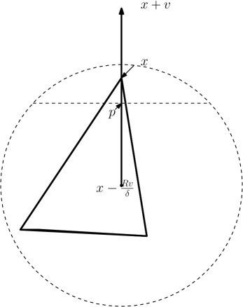
Figure 5: The $D$-dimensional ball with center $x-\frac{Rv}{{\mathbf{\delta}}}$ and radius $\frac{R}{{\mathbf{\delta}}}+{\epsilon}$ contains the convex set $K$ (depicted above as a triangle).

11.1 Final Optimization

We recall the definition of a Weak Optimization Problem (Definition 7.1):
Given a vector $v\in\mathbb{Q}^{n},$ and a rational number ${\epsilon}>0$, either

1. find a vector $y\in\mathbb{Q}^{n}$ such that $y\in S(K,{\epsilon})$ and $v^{T}x\leq v^{T}y+{\epsilon}$ for all $x\in S(K,-{\epsilon}),$ or

2. assert that $S(K,-{\epsilon})$ is empty.

We recall also the definition of a Weak Validity Problem (Definition 7.2):
Given a vector $c\in\mathbb{Q}^{n},$ a rational number $\gamma$, and a rational number ${\epsilon}>0$, either

1. assert that $c^{T}x\leq\gamma+{\epsilon}$ for all $x\in S(K,-{\epsilon}),$ or

2. assert that $c^{T}x\geq\gamma-{\epsilon}$ for some $x\in S(K,{\epsilon})$
   (i. e., $c^{T}x\leq\gamma$ is almost invalid).

Given an oracle that solves a Weak Validity Problem, [52] shows how the ellipsoid algorithm can be used to solve a Weak Optimization Problem with a polynomial run-time. Note that this algorithm calls the algorithm Find-distance polynomially many times. We assume that it uses in each step, new, independently chosen sample points. We denote by $\pi^{alg}_{\epsilon}(v)$, the (random) output of the algorithm that takes as input, the vector $v$ and a threshold ${\epsilon}$, and outputs a corresponding solution of the Weak Optimization Problem. Note that this output is random because the oracle it queries, uses random samples from $\mu\ast G_{\sigma}^{(D)}.$

We will now show that if a vector $v\in B_{1}^{D}(0)\cap\pi^{-1}(x)$ is the center of a $(D-d)$-dimensional ${\mathbf{\delta}}$-ball contained in $B_{1}^{D}(0)\cap\pi^{-1}(x),$ then the ellipsoid algorithm for solving the weak optimization problem with objective $v$ outputs a point $y$ that is close to $x$ in the Euclidean norm.

Lemma 11.1.

If a unit vector $v_{p}\in\pi^{-1}(p)$ is the center of a $(D-d)$-dimensional ${\mathbf{\delta}}$-ball contained in $\pi^{-1}(p),$ then, the $D$-dimensional ball with center $p-\frac{Rv_{p}}{{\mathbf{\delta}}}$ and radius $\frac{R}{{\mathbf{\delta}}}$ contains $K$, i. e.

$$B^{D}_{{R}/{{\mathbf{\delta}}}}\left(p-\frac{Rv_{p}}{{\mathbf{\delta}}}\right)\supseteq K.$$

Proof.

We know that

$$\forall q\in\mathcal{M}\ \forall v_{1}\in(T_{p}\mathcal{M})^{\perp}:\,\,\langle q-p,v_{p}+{\mathbf{\delta}}v_{1}\rangle\leq 0.$$ (131)

Fix $q\in\mathcal{M}.$ Then, $v^{\prime}$ belongs to the closure of $\mathfrak{N}(q).$ Let

$$v_{1}:=\frac{\Pi_{(T_{p}\mathcal{M})^{\perp}}(q-p)}{\|\Pi_{(T_{p}\mathcal{M})^{\perp}}(q-p)\|}.$$

Then by (131) and by using Lemma 3.2 in (134),

$$\langle q-p,-v_{p}\rangle \geq \langle q-p,{\mathbf{\delta}}v_{1}\rangle$$ (132)

$$= {\mathbf{\delta}}\|\Pi_{(T_{p}\mathcal{M})^{\perp}}(q-p)\|$$ (133)

$$\geq {\mathbf{\delta}}\left(\frac{1}{2R}\right)\|q-p\|^{2}.$$ (134)

This gives us

$$\|q-(p-(R/{\mathbf{\delta}})v_{p})\|^{2} = \|q-p\|^{2}+(R/{\mathbf{\delta}})^{2}-\langle q-p,-2(R/{\mathbf{\delta}})v_{p}\rangle$$ (135)

$$\leq \|q-p\|^{2}+(R/{\mathbf{\delta}})^{2}-\|q-p\|^{2}$$ (136)

$$= (R/{\mathbf{\delta}})^{2}.$$ (137)

Since this applies to an arbitrary point $q\in\mathcal{M},$ it proves the lemma. ∎

Let $v_{i}\in B^{D}_{1}(0)\setminus(B^{D}_{1-2{\mathbf{\delta}}}(0)).$

Definition 11.1.

Let $x_{i}=x_{v_{i}}$ be a maximizer of $\langle x,v_{i}\rangle$ over $\mathcal{M}$, which is chosen arbitrarily in case there is more than one maximizer.

Let $p_{i}$ be the point $x_{i}-\frac{{\epsilon}v_{i}}{\|v_{i}\|}.$ Consider the halfspace

$$H_{p_{i}}=\{{\color[rgb]{0,0,0}y\in\mathbb{R}^{D}}\,|\,\langle(y-p_{i}),v_{i}\rangle\geq 0\}.$$

Lemma 11.2.

A solution $y_{i}$ of the Weak Optimization Problem which $c{\epsilon}$-approximately maximizes $\langle v_{i},z\rangle$ over $z\in K,$ satisfies $\|y_{i}-x_{i}\|<C\sqrt{\frac{{\epsilon}R}{{\mathbf{\delta}}_{i}}}.$

Proof.

The diameter of $B^{D}_{\frac{R}{{\mathbf{\delta}}_{i}}+{\epsilon}}\left(x_{i}-\frac{Rv_{i}}{{\mathbf{\delta}}_{i}\|v\|}\right)\cap H_{p_{i}}$ is bounded above by $C\sqrt{\frac{{\epsilon}R}{{\mathbf{\delta}}_{i}}}.$ Since $x_{i}$ belongs to this set, the lemma follows. By Lemma 7.2, the point $y_{i}$ which $c{\epsilon}$-approximately maximizes $\langle v_{i},z\rangle$ over $z\in K$ belongs to

$$S(K,-{\epsilon})\cap H_{p_{i}}\subseteq B^{D}_{\frac{R}{{\mathbf{\delta}}_{i}}+{\epsilon}}\left(x_{i}-\frac{Rv_{i}}{{\mathbf{\delta}}_{i}\|v_{i}\|}\right)\cap H_{p_{i}}.$$

Therefore, the point $y_{i}$ satisfies $\|y-x_{i}\|<C\sqrt{\frac{{\epsilon}R}{{\mathbf{\delta}}_{i}}}.$ ∎

11.2 Algorithm for identifying good choices of $v$.

Figure 6: There is at least one point $i\in[\mathcal{N}]$, such that ${\mathbf{\delta}}_{i}>cr_{1}{\mathbf{\delta}}.$ The convex set represents a two dimensional cross section of $\mathfrak{N}_{K}(x_{v}).$ The balls depicted are the intersections of the affine span of this cross section with the the $D$-dimensional balls refered to in the picture above.

We also need a procedure that handles the situation when $r_{0}$ is small, i. e. when $v$ is close to the boundary of the outer normal cone it belongs to. This procedure must exclude cases when the point output by the optimization routine applied to $v\in\mathbb{R}^{D}$ is far from the base point of the fiber containing $v$. Let $r_{1}$ be an a priori lower bound on the radius of the largest $(D-d)$-dimensional ball contained in $\mathfrak{N}_{K}(x),$ for any $x\in\mathcal{M}.$ Note that by Lemma 9.7, $N_{K}(x)$ contains a $(D-d)$-dimensional ball of radius $\frac{\tau}{R},$ centered at a unit vector, and so rescaling that vector multiplicatively by $\frac{1}{1+({\tau}/{R})},$ we see that we may take

$$r_{1}:=\frac{\tau}{\tau+R}.$$ (138)

Let

$$r_{0}:=\frac{r_{1}}{2}.$$ (139)

We choose ${\mathbf{\delta}}$ given by

$${\mathbf{\delta}}=\min\left(\left(\frac{{\epsilon}}{2RL^{2}}\right)^{\frac{1}{3}},\left(\frac{r_{0}^{2}}{RL}+1\right)r_{0}\right).$$

As a consequence,

$$\left(\frac{RL}{r_{0}^{2}}\right){\mathbf{\delta}}=\min\left(\sqrt{\frac{{\epsilon}R}{r_{1}{\mathbf{\delta}}}},\left(\frac{RL}{r_{0}^{2}}+1\right)r_{0}\right).$$ (140)

Let

$${\epsilon}^{\prime}:=\frac{r_{1}}{4L},$$ (141)

where $L$ is the Lipschitz constant appearing in Theorem 6.1. Let $\{v_{i}|i\in[\mathcal{N}]\}$ be an ${\epsilon}^{\prime}{\mathbf{\delta}}$-net of the sphere $\partial B_{\mathbf{\delta}}^{D}((1-{\mathbf{\delta}})v)$. (Note that $x_{i}=x_{v_{i}}$ is in general not equal to $x_{v}$.)

For each $i\in[\mathcal{N}]$, let ${\mathbf{\delta}}_{i}$ be the largest nonnegative real number ${\mathbf{\delta}}^{\prime}$ such that $B^{D}_{{\mathbf{\delta}}^{\prime}}(v_{i})\cap(T_{x_{i}}\mathcal{M})^{\perp}\subseteq\mathfrak{N}_{K}(x_{i}).$

Lemma 11.3.

1. There is at least one index $i\in[\mathcal{N}]$, such that ${\mathbf{\delta}}_{i}>cr_{1}{\mathbf{\delta}}.$

2. If $v$ is at a distance greater than $r_{0}$ from $\partial N_{k}(x_{v}),$ for every index $i\in[\mathcal{N}]$, we have ${\mathbf{\delta}}_{i}>cr_{1}{\mathbf{\delta}}.$

Proof.

Let $\overline{v}$ denote a point in $\mathfrak{N}_{K}(x)$ that is the center of a $(D-d)$-dimensional ball contained in $\mathfrak{N}_{K}(x)$ of radius $r_{1}.$ Let

$$v^{\prime}:=\partial B_{\mathbf{\delta}}^{D}((1-{\mathbf{\delta}})v)\cap\{\lambda\overline{v}+(1-\lambda)(1-{\mathbf{\delta}})v|\lambda\in[0,1]\}.$$

Thus, $v^{\prime}$ is the intersection of the line segment joining $\overline{v}$ and $(1-{\mathbf{\delta}})v,$ with $\partial B_{\mathbf{\delta}}^{D}((1-{\mathbf{\delta}})v).$ Since $(1-{\mathbf{\delta}})v$ and $\overline{v}$, both belong to $\mathfrak{N}(x),$ it follows from the convexity of $\mathfrak{N}(x),$ and the fact that $\|(1-{\mathbf{\delta}})v-\overline{v}\|<2$ that

$$B_{{r_{1}{\mathbf{\delta}}}/{2}}^{D}(v^{\prime})\cap(T_{x}\mathcal{M})^{\perp}\subseteq\mathfrak{N}(x).$$

Let $v_{j}$ be a point in $\{v_{i}|i\in[\mathcal{N}]\}$ at a minimal distance from $v^{\prime}$. By Theorem 6.1 we know that the the variation of $\mathfrak{N}_{K}(x)$ as a function of $x,$ measured in Hausdorff distance, is $L$-Lipschitz. Since ${\epsilon}^{\prime}=\frac{r_{1}}{4L},$ it follows that ${\mathbf{\delta}}_{j}>cr_{1}{\mathbf{\delta}}.$ This proves part 1. of the lemma. To see part 2. of the lemma, note that if $v$ is at a distance greater than $r_{0}$ from $\partial N_{k}(x_{v}),$ by (140), ${\mathbf{\delta}}<r_{0},$

$$\partial B_{{\mathbf{\delta}}(1-{\mathbf{\delta}})}^{D}((1-{\mathbf{\delta}})v)\cap(T_{x}\mathcal{M})^{\perp}\subseteq\mathfrak{N}(x),$$

and so we are done by Theorem 6.1. ∎

Recall that $r_{0}=\frac{\tau}{2\tau+2R}$ by (139).

Lemma 11.4.

Let $v$ be sampled from the uniform probability measure on $\partial B_{1}(0).$ Then,

$$\mathbb{P}\left[dist(v,\partial N_{K}(x_{v}))\geq r_{0}\right]\geq 2^{-2D}\left(\frac{\tau}{R}\right)^{D+d}.$$

Proof.

Let

$$G:=\left\{v\in B_{1}(0)\big{|}\,dist\left(\frac{v}{\|v\|},\partial N_{K}(x_{v})\right)\geq r_{0}\right\}.$$

By Lemma 9.6,

$$\frac{\mathrm{vol}_{D}(G)}{\omega_{D}}\geq\left(\frac{r_{0}\tau}{R}\right)^{d}\inf_{p\in\mathcal{M}}\frac{\mathrm{vol}_{D-d}(\mathfrak{N}_{K}(p)\cap G)}{\mathrm{vol}_{D-d}(\mathfrak{N}_{K}(p))}.$$

By (138) and (139), we see that for all $p\in\mathcal{M}$, $\mathfrak{N}_{K}(p)\cap G$ contains a $(D-d)$-dimensional ball of radius $r_{0}$, and therefore,

$$\left(\frac{r_{0}\tau}{R}\right)^{d}\inf_{p\in\mathcal{M}}\frac{\mathrm{vol}_{D-d}(\mathfrak{N}_{K}(p)\cap G)}{\mathrm{vol}_{D-d}(\mathfrak{N}_{K}(p))}\geq r_{0}^{D}\left(\frac{\tau}{R}\right)^{d}.$$

Substituting the value of $r_{0}=\frac{\tau}{2\tau+2R}\geq\frac{\tau}{4R},$ the Lemma follows. ∎

Let us assume that ${\epsilon}<\frac{c\tau}{d}.$ Let

$$\mathcal{N}_{0}=\left\lceil\left(\frac{4R}{\tau}\right)^{D+d}\left(\frac{V}{\omega_{d}{\epsilon}^{d}}\right)\right\rceil.$$ (142)

Let $\eta\in(0,1)$ be a parameter that bounds from above the probability with which the algorithm is permitted to fail.

11.3 Algorithm Find-points

Algorithm Find-points

Input parameters: ${\epsilon}>0$, $D,\mathcal{N},p,\mathcal{N}_{0},\in\mathbb{Z}_{+}$ and the sample points $X_{1},X_{2},\dots,X_{N_{3}}\in\mathbb{R}^{D}$, where $N_{3}=p\mathcal{N}_{0}\mathcal{N}$.

1. For $1\leq j\leq\mathcal{N}_{0},$ do the following.

   1. Let $v^{(j)}$ be sampled from the uniform measure on $\partial B_{1}(0).$

   2. Let $\{v^{(j)}_{i}|i\in[\mathcal{N}]\}$ be an ${\epsilon}^{\prime}{\mathbf{\delta}}$-net of the sphere $\partial B_{\mathbf{\delta}}^{D}((1-{\mathbf{\delta}})v^{(j)})$.

   3. Use the algorithm Weak-Optimization-Oracle to find the solution $y_{i}^{(j)}$ for the Weak Optimization Problem which $c{\epsilon}$-approximately maximizes $\langle v_{i}^{(j)},z\rangle$ over $z\in K,$ for each $i\in[\mathcal{N}].$ This step uses $p$ samples. If any of the algorithms Weak-Optimization-Oracle fail, output that the algorithm has failed, otherwise proceed to the next step.

   4. If we have $\|y_{1}^{(j)}-y_{i}^{(j)}\|<C\sqrt{\frac{{\epsilon}R}{r_{1}{\mathbf{\delta}}}},$ for each $i\in[\mathcal{N}]$, then output $y^{(j)}:=y_{1}^{(j)}$, otherwise output no point and declare that $v^{(j)}$ is within $r_{0}$ of $\partial N_{K}(\pi(v^{(j)})).$

Lemma 11.5.

The number $N_{3}$ of the needed sample points $X_{i}$, $i=1,2,\dots,N_{3}$ as well as the number of the arithmetic operations performed during the execution of the algorithm Find-points is bounded above by

$$\mathcal{N}\mathcal{N}_{0}\exp\left(\tilde{\Omega}\left(\left(\frac{RL\sigma}{{\epsilon}\tau^{2}}\log\frac{V}{\tau^{d}}\right)^{2}\right)\right)\log\left(\eta^{-1}\right).$$ (143)

where $L\leq CR(\Lambda+\tau^{-2})$ is the constant from the statement of Theorem 6.1.

Proof.

Recall (see the algorithm Find-Distance, formula (8.1)) that in order to get a uniform additive estimate on $\Gamma(H_{\gamma^{\prime},b},\frac{{\epsilon}}{RL})/|\mathcal{M}|$ to within an accuracy of

$$\mathbf{a}:=\frac{c{\epsilon}}{RL}\frac{1}{V}\Gamma_{{\epsilon}/({RL})},$$

with probability greater than $1-{\eta_{1}}$, it suffices to take $N$ samples, where

$$N\mathbf{a}^{2} \geq C\log\left({\eta_{1}}^{-1}(N/D)^{D}\right)$$ (144)

$$= C\log{\eta_{1}}^{-1}+CD\log\frac{N}{D}.$$ (145)

This is satisfied for

$$N=\tilde{\Omega}\left(\mathbf{a}^{-2}D+\mathbf{a}^{-2}\log{\eta_{1}}^{-1}\right),$$ (146)

which can be bounded above by

$$\exp\left(\tilde{\Omega}\left(\left(\frac{RL\sigma}{{\epsilon}\tau}\log\frac{V}{\tau^{d}}\right)^{2}\right)\right)\log\left({\eta_{1}}^{-1}\right).$$

When we use $\eta_{1}=\frac{\eta}{\mathcal{N}\mathcal{N}_{0}}$, the each use of the algorithm Find-Distance, called in the algorithn Weak-Optimization-Oracle, outputs a correct solution at least with probability $1-\frac{\eta}{\mathcal{N}\mathcal{N}_{0}}$. As the algorithm Find-Distance is called at most ${\mathcal{N}\mathcal{N}_{0}}$ times, this yields that algorithm Find-points outputs correct solutions at least with probability $1-\eta$. This proves the claim. ∎

For constant values for the parameters $\sigma,R,\Lambda,\tau,V,\eta,{\epsilon}$ and $d<c\sqrt{\log\log n},$ this bound is dominated by the contribution of $\mathcal{N}_{0}$, which is bounded by $\exp\left(CD\log\frac{R}{\tau}\right)<n^{C},$ where we recall that $D<\left(\frac{CV}{\tau^{d}}\right)^{\frac{d}{2}+1}.$ For the purposes of analysis of the algorithm, we isolate the following subroutine, consisting of parts (c) and (d) of find-points, which we term the ${\mathbf{\delta}}$-ball tester.

11.4 Algorithm ${\mathbf{\delta}}$-ball tester

Algorithm ${\mathbf{\delta}}$-ball tester

Input parameters: ${\epsilon}>0$, $D,p,N\in\mathbb{Z}_{+}$ and the sample points $X_{1},X_{2},\dots,X_{\mathcal{N}_{4}}\in\mathbb{R}^{D}$, where $\mathcal{N}_{4}=\mathcal{N}p$.

1. For each $i\in[\mathcal{N}]$, use the algorithm Find-points to find the solutions $y_{i}$ of the Weak Optimization Problem which $c{\epsilon}$-approximately maximizes $\langle v_{i},z\rangle$ over $z\in K$. This step uses $p$ samples. If any of the algorithms Find-points fails, output that the algorithm ${\mathbf{\delta}}$-ball tester has failed, otherwise proceed to the next step.

2. If we have $\|y_{1}-y_{i}\|<C\sqrt{\frac{{\epsilon}R}{r_{1}{\mathbf{\delta}}}},$ for each $i\in[\mathcal{N}]$, then output $y_{1}$, otherwise output no point and declare that $v$ is within $r_{0}$ of $\partial N_{K}(x_{v}).$

Theorem 11.6.

The ${\mathbf{\delta}}$-ball tester takes as input $v\in\partial B_{1}(0)$ and returns an output that satisfies the following properties.

1. If $v$ is at a distance greater than $r_{0}$ from $\partial N_{K}(x_{v}),$ it returns a point $y_{1}$ that is $C\sqrt{\frac{{\epsilon}R}{r_{1}{\mathbf{\delta}}}}$-close to $x_{v}.$

2. If $v$ is at a distance less or equal to $r_{0}$ from $\partial N_{K}(x_{v}),$ it either returns a point $y_{1}$ that is $C\sqrt{\frac{{\epsilon}R}{r_{1}{\mathbf{\delta}}}}$-close to $x_{v}$, or outputs no point, together with a declaration that $v$ is within $r_{0}$ of $\partial N_{K}(x_{v}).$

Proof.

The ${\mathbf{\delta}}$-ball tester returns the point $y_{1}$ corresponding to $v_{1}$ if and only if $\|y_{1}-y_{i}\|<C\sqrt{\frac{{\epsilon}R}{r_{1}{\mathbf{\delta}}}},$ for each $i\in[\mathcal{N}]$, otherwise it returns no point and a declaration of error. If $v$ is at a distance greater than $r_{0}$ from $\partial N_{K}(x_{v}),$ by Lemma 10.1, for every $v^{\prime\prime}\in B^{D}_{{\mathbf{\delta}}}((1-{\mathbf{\delta}})v),$

1. $\|x_{v^{\prime\prime}}-x_{v}\|<\left(\frac{CRL}{r_{0}^{2}}\right){\mathbf{\delta}}.$

2. $v^{\prime\prime}$ is the center of a $(D-d)$-dimensional ball of radius $\frac{r_{0}}{2}$ contained in $N_{K}(x_{v^{\prime\prime}}).$

These facts, together Lemma 11.2, imply that for every $v_{i},i\in[\mathcal{N}]$ we have that the solution $y_{i}$ of the Weak Optimization Problem which $c{\epsilon}$-approximately maximizes $\langle v_{i},z\rangle$ over $z\in K,$ satisfies $\|y_{i}-x_{i}\|<C\sqrt{\frac{{\epsilon}R}{{\mathbf{\delta}}_{i}}},$ where by Lemma 11.3, ${\mathbf{\delta}}_{i}>cr_{1}r_{0}>cr_{1}{\mathbf{\delta}}$ This proves part 1. of this theorem. To see part 2., we apply part 1. of Lemma 11.3, together with Lemma 11.2, and observe in view of (140), that there exists a $y_{j}$ that is $C\sqrt{\frac{{\epsilon}R}{r_{1}{\mathbf{\delta}}}}$-close to $x_{v}.$ A necessary condition for the ${\mathbf{\delta}}$-ball tester returning a point, is that this point $y_{j}$ is $C\sqrt{\frac{{\epsilon}R}{r_{1}{\mathbf{\delta}}}}$-close to $y_{1}.$ Therefore, if a point is returned, that point must be $C\sqrt{\frac{{\epsilon}R}{r_{1}{\mathbf{\delta}}}}$-close to $x_{v}.$ ∎

Corollary 11.7.

With probability greater or equal to $1-C\eta$, the output of find-points is a $C\sqrt{\frac{{\epsilon}R}{r_{1}{\mathbf{\delta}}}}$ net of $\mathcal{M}_{0}$, which we call $\mathcal{X}_{1}.$

12 Implicit description of output manifold $\mathcal{M}_{\color[rgb]{0,0,0}rec}$

Let ${\epsilon}^{\prime\prime}:=C\sqrt{\frac{{\epsilon}R}{r_{1}{\mathbf{\delta}}}}.$ Plugging the above corollary into subsection 5.5 of [45], and using the results in Sections 6 and 7 of that paper, we obtain an algorithm that computes an implicit description of a manifold $\mathcal{M}_{\color[rgb]{0,0,0}rec}$ of reach greater than $c\tau/d^{6}$ such that $d_{H}(\mathcal{M}_{\color[rgb]{0,0,0}rec},\mathcal{M})<Cd{\epsilon}^{\prime\prime}.$ We give a brief overview of how this is done, below. A subnet $\mathcal{X}_{2}$ at a scale $\frac{c\tau}{d}$ of the net $\mathcal{X}_{1}$ is fed into a subroutine $FindDisc$ below and as an output we obtain a family of discs of dimension $d$ that cover $\mathcal{M}_{0}$ in the sense that the $n$-dimensional balls with the same centers and radii, cover $\mathcal{M}.$ These discs are fine-tuned as mentioned below.

12.1 $FindDisc$

Algorithm FindDisc

Input: Set $X_{0}$.

1. Let $x_{1}$ be a point that minimizes $|1-|x-x^{\prime}||$ over all $x^{\prime}\in X_{0}$.

2. Given $x_{1},\dots x_{m}$ for $m\leq d-1$, choose $x_{m+1}$ such that

   $$\max(|1-|x-x^{\prime}||,|\langle x_{1}/|x_{1}|,x^{\prime}\rangle|,\dots,|\langle x_{m}/|x_{m}|,x^{\prime}\rangle|)$$

   is minimized among all $x^{\prime}\in X_{0}$ for $x^{\prime}=x_{m+1}$.

Output points $x_{1},\dots x_{d}$.

We start with a putative of tangent disc on a point of the net using $FindDisc.$ This is fine tuned to get essentially optimal tangent disc as follows. We view the tangent disc locally as the graph of a linear function for data and obtain a nearly optimal linear function using convex optimization, with quadratic loss as the objective, and the domain being a convex set parameterizing the flats near the putative flat.

12.2 Bump functions

For each center $p_{i}$ of each output disc of radius $r$, consider the bump function $\tilde{\alpha}_{i}(x)$ given by

$$\tilde{\alpha}_{i}(p_{i}+rv)=c_{i}(1-\|v\|^{2})^{d+2},$$

for any $v\in B_{n}$ and $0$ otherwise. Let

$$\tilde{\alpha}(x):=\sum_{i}\tilde{\alpha}_{i}(x).$$

Let

$$\alpha_{i}(x)=\frac{\tilde{\alpha}_{i}(x)}{\tilde{\alpha}(x)}$$

for each $i.$

12.3 Weights

It is possible to choose $c_{i}$ such that for any $z$ in a $\frac{r}{4d}$ neighborhood is $\mathcal{M}$,

$$c^{-1}>\tilde{\alpha}(z)>c,$$

where $c$ is a small universal constant. Further, such $c_{i}$ can be computed using no more than $|\mathcal{X}_{1}|(Cd)^{2d}$ operations involving vectors of dimension $D.$

12.4 An approximate gradient of the squared distance function

We consider the scaled setting where $r=1$. Thus, in the new Euclidean metric, $\tau\geq Cd^{C}$. Let $\Pi^{i}$ be the orthogonal projection of $\mathbb{R}^{n}$ onto the $(n-d)-$dimensional subspace containing the origin that is orthogonal to the affine span of $D_{i}$. Recall that the $p_{i}$ are the centers of the discs $D_{i}$ as $i$ ranges over $[N_{3}]$. We define the function $F_{i}:U_{i}\rightarrow\mathbb{R}^{n}$ by $F_{i}(x)=\Pi^{i}(x-p_{i})$. Let $\cup_{i}U_{i}=U$. We define $F:U\rightarrow\mathbb{R}^{n}$ by

$$F(x)=\sum_{i\in[N_{3}]}\alpha_{i}(x)F_{i}(x).$$ (147)

Figure 7: Using data from the net, we construct an output manifold. The grey lines represent fibers of a certain approximate extension of the normal bundle of $\mathcal{M}$, that is used to construct the output manifold. The manifold itself is defined by an equation of the form $\Pi_{x}F(x)=0$ where $\Pi_{x}$ is an orthogonal projection on to the fiber at $x$, and $F$ is a certain vector valued function.

12.5 An approximate (extension of) the normal bundle to a base that is a tubular neighborhood of $\mathcal{M}$

Given a symmetric matrix $A$ such that $A$ has $n-d$ eigenvalues in $(1/2,3/2)$ and $d$ eigenvalues in $(-1/2,1/2)$, let $\Pi_{hi}(A)$ denote the projection in $\mathbb{R}^{n}$ onto the span of the eigenvectors of $A$, corresponding to the largest $n-d$ eigenvalues.

Definition 12.1.

For $x\in\cup_{i}U_{i}$, we define $\Pi_{x}=\Pi_{hi}(A_{x})$ where $A_{x}=\sum_{i}\alpha_{i}(x)\Pi^{i}$.

12.6 The output manifold

Let $\widetilde{U}_{i}$ be defined as the $\frac{cr}{d}-$Eucidean neighborhood of $D_{i}$ intersected with $U_{i}$. Given a matrix $X$, its Frobenius norm $\|X\|_{F}$ is defined as the square root of the sum of the squares of all the entries of $X$. This norm is unchanged when $X$ is premultiplied or postmultiplied by orthogonal matrices (of the appropriate order). Note that $\Pi_{x}$ is $\mathcal{C}^{2}$ when restricted to $\bigcup_{i}\widetilde{U}_{i}$, because the $\alpha_{i}(x)$ are $\mathcal{C}^{2}$ and when $x$ is in this set, $c<\sum_{i}\widetilde{\alpha}_{i}(x)<c^{-1}$, and for any $i,j$ such that $\alpha_{i}(x)\neq 0\neq\alpha_{j}(x)$, we have $\|\Pi^{i}-\Pi^{j}\|_{F}<Cd{\mathbf{\delta}}$.

Definition 12.2.

Let $F_{\color[rgb]{0,0,0}rec}(x)=\Pi_{x}(F(x))$, where $F$ and $\Pi_{x}$ are constructed in formula (147) and Definition 12.1. The output manifold $\mathcal{M}_{\color[rgb]{0,0,0}rec}$ is the set of all points $x\in\bigcup_{i}\widetilde{U}_{i}$ such that $F_{\color[rgb]{0,0,0}rec}(x)=0$, that is,

$$\mathcal{M}_{\color[rgb]{0,0,0}rec}=\{x\in\mathbb{R}^{n}\ |\ F_{\color[rgb]{0,0,0}rec}(x)=0\}.$$ (148)

12.7 Analysis of reach

Thus $\mathcal{M}_{\color[rgb]{0,0,0}rec}$ is the set of points $x\in\bigcup_{i}\widetilde{U_{i}}$ such that

$$\Pi_{hi}(\sum_{i\in[N_{3}]}\alpha_{i}(x)\Pi^{i})(\sum_{i\in[N_{3}]}\alpha_{i}(x)\Pi^{i}(x-p_{i}))=0$$

and

$$\Pi_{hi}(\sum_{i}\alpha_{i}(x)\Pi^{i})=\frac{1}{2\pi i}\left[\oint_{\gamma}(zI-(\sum_{i}\alpha_{i}(x)\Pi^{i}))^{-1}dz\right]$$

using diagonalization and Cauchy’s integral formula, and so

$$\frac{1}{2\pi i}\left[\oint_{\gamma}(zI-(\sum_{i}\alpha_{i}(x)\Pi^{i}))^{-1}dz\right]\left(\sum_{i}\alpha_{i}(x)\Pi^{i}(x-p_{i})\right)=0$$

where $\gamma$ is the circle of radius $1/2$ centered at $1$. The proof of the bound on the reach (Theorem 7.4 in [45]) hinges on the above representation.

12.8 Final result

The additional computational cost in going from the net to $\mathcal{M}_{\color[rgb]{0,0,0}rec}$ is exponential in $D$, nearly linear in $n$, and polynomial in $1/{\epsilon}^{\prime\prime}$. These and the above considerations prove Theorem 1.1.

13 Open questions and remarks

1. Can any of the following constraints be relaxed while allowing the parameters $\sigma,R,\Lambda,\tau,V,\eta,{\epsilon}$ to be arbitrary constants independent of $n$, and preserving the polynomial time guarantee?

   • $\mathcal{M}\subseteq\partial K$ ?

   • $d<c\sqrt{\log\log n}.$

2. Can the guarantee on the reach of the output manifold be improved? We currently have $\mathrm{reach}(\mathcal{M}_{\color[rgb]{0,0,0}rec})\geq\frac{C\tau}{d^{6}}.$

14 Acknowledgements

We are grateful to Somnath Chakraborty for several helpful discussions.

Ch.F. was partly supported by the US-Israel Binational Science Foundation grant number 2014055, AFOSR grant FA9550- 12-1-0425 and NSF grant DMS-1265524. S.I. was partly supported RFBR grant 20-01-00070, M.L. was supported by PDE-Inverse project of the European Research Council of the European Union and Academy of Finland, grants 273979 and 284715, and H.N. was partly supported by a Swarna Jayanti fellowship and the Infosys-Chandrasekharan virtual center for Random Geometry. Views and opinions expressed are those of the authors only and do not necessarily reflect those of the European Union or the other funding organizations. Neither the European Union nor the other funding organizations can be held responsible for them.

Appendix A Some auxiliary lemmas from [45]

Lemma A.1 (Lemma A.1 [45]).

Suppose that $\mathcal{M}$ is a compact $d$-dimensional embedded $\mathcal{C}^{2}$-submanifold of $\mathbb{R}^{m}$ whose volume is at most $V$ and reach is at least $\tau.$ Let

$$U:=\{y\in\mathbb{R}^{m}\big{|}|y-\Pi_{x}y|\leq\tau/4\}\cap\{y\in\mathbb{R}^{m}\big{|}|x-\Pi_{x}y|\leq\tau/4\}.$$

Then,

$$\Pi_{x}(U\cap\mathcal{M})=\Pi_{x}(U).$$

Lemma A.2 (Lemma A.2 [45]).

Suppose that $\mathcal{M}\in\mathcal{G}(d,m,V,\tau)$. Let $x\in\mathcal{\mathcal{M}}$ and

$$\widehat{U}:=\{y\in\mathbb{R}^{m}\big{|}|y-\Pi_{x}y|\leq\tau/8\}\cap\{y\in\mathbb{R}^{m}\big{|}|x-\Pi_{x}y|\leq\tau/8\}.$$

There exists a $C^{2}$ function $F_{x,\widehat{U}}$ from $\Pi_{x}(\widehat{U})$ to $\Pi_{x}^{-1}(\Pi_{x}(0))$ such that

$$\{y+F_{x,\widehat{U}}(y)\big{|}y\in\Pi_{x}(\widehat{U})\}=\mathcal{M}\cap\widehat{U}.$$

Secondly, for ${\mathbf{\delta}}\leq\tau/8$, let $z\in\mathcal{M}\cap\widehat{U}$ satisfy $|\Pi_{x}(z)-x|={\mathbf{\delta}}.$ Let $z$ be taken to be the origin and let the span of the first $d$ canonical basis vectors be denoted $\mathbb{R}^{d}$ and let $\mathbb{R}^{d}$ be a translate of $Tan(x)$. Let the span of the last $m-d$ canonical basis vectors be denoted $\mathbb{R}^{m-d}$. In this coordinate frame, let a point $z^{\prime}\in\mathbb{R}^{m}$ be represented as $(z^{\prime}_{1},z^{\prime}_{2})$, where $z^{\prime}_{1}\in\mathbb{R}^{d}$ and $z^{\prime}_{2}\in\mathbb{R}^{m-d}$. By Lemma 8.2, there exists an $(m-d)\times d$ matrix $A_{z}$ such that

$$Tan(z)=\{(z^{\prime}_{1},z^{\prime}_{2})|A_{z}z^{\prime}_{1}-Iz^{\prime}_{2}=0\}$$ (149)

where the identity matrix is $(m-d)\times(m-d)$. Let $z\in\mathcal{M}\cap\{z\big{|}|z-\Pi_{x}z|\leq{\mathbf{\delta}}\}\cap\{z\big{|}|x-\Pi_{x}z|\leq{\mathbf{\delta}}\}$. Then $\|A_{z}\|_{2}\leq 15{\mathbf{\delta}}/\tau.$ Lastly, the following upper bound on the second derivative of $F_{x,\widehat{U}}$ holds for $y\in\Pi_{x}(\widehat{U})$.

$$\forall{v\in\mathbb{R}^{d}}\ \forall{w\in\mathbb{R}^{m-d}}:\ \ \langle\partial_{v}^{2}F_{x,\widehat{U}}(y),w\rangle\leq\frac{C|v|^{2}|w|}{\tau}.$$

References

- [1] E. Aamari, E., and C. Levrard, Nonasymptotic rates for manifold, tangent space and curvature estimation. Ann. Statist. 47, 1 (02 2019), 177–204.
- [2] M. Anderson, Convergence and rigidity of manifolds under Ricci curvature bounds, Invent. Math. 102 (1990), 429–445.
- [3] Y. Aizenbud, Y., and B. Sober, (2021). Non-Parametric Estimation of Manifolds from Noisy Data. https://arxiv.org/abs/2105.04754
- [4] J. Boissonnat, L. J. Guibas, and S. Oudot, Manifold reconstruction in arbitrary dimensions using witness complexes. Discrete & Computational Geometry 42, 1 (2009), 37–70.
- [5] S. Boucheron, O. Bousquet and G. Lugosi, Theory of classification : a survey of some recent advances, ESAIM: Probability and Statistics, 9 (2005), 323–375.
- [6] M. Belkin, P. Niyogi, Laplacian eigenmaps and spectral techniques for embedding and clustering, Adv. in Neural Inform. Process. Systems, 14 (2001), 586–691.
- [7] M. Belkin, P. Niyogi, Semi-Supervised Learning on Riemannian Manifolds, Machine Learning, 56 (2004), 209–239.
- [8] M. Belkin, P. Niyogi, Convergence of Laplacian eigenmaps, Adv. in Neural Inform. Process. Systems 19 (2007), 129–136.
- [9] V. Berestovskij, I. Nikolaev, Multidimensional generalized Riemannian spaces, In: Geometry IV, Encyclopaedia Math. Sci. 70, Springer, 1993, pp. 165–243.
- [10] E. Beretta, M. de Hoop, L. Qiu, Lipschitz Stability of an Inverse Boundary Value Problem for a Schrödinger-Type Equation SIAM J. Math. Anal. 45 (2012), 679-699.
- [11] E. Bierstone, P. Milman, W. Paulucki, Differentiable functions defined on closed sets. A problem of Whitney, Invent. Math., 151 (2003), 329–352.
- [12] J. Boissonnat, L. Guibas, S. Oudot, Manifold reconstruction in arbitrary dimensions using witness complexes, Discrete Computational Geometry 42 (2009), 37–70.
- [13] S. Bromberg, An extension in the class , Bol. Soc. Mat. Mex. II, Ser. 27, (1982), 35–44.
- [14] Y. Brudnyi, On an extension theorem, Funk. Anal. i Prilzhen. 4 (1970), 97–98; English transl. in Func. Anal. Appl. 4 (1970), 252–253.
- [15] Y. Brudnyi, P. Shvartsman, The traces of differentiable functions to closed subsets of , in Function Spaces (1989), Teubner-Texte Math. 120, 206–210.
- [16] Y. Brudnyi, P. Shvartsman, A linear extension operator for a space of smooth functions defined on closed subsets of , Dokl. Akad. Nauk SSSR 280 (1985), 268–270. English transl. in Soviet Math. Dokl. 31, No. 1 (1985), 48–51.
- [17] Y. Brudnyi, P. Shvartsman, Generalizations of Whitney’s extension theorem, Int. Math. Research Notices 3 (1994), 129–139.
- [18] Y. Brudnyi, P. Shvartsman, The traces of differentiable functions to closed subsets of , Dokl. Akad. Nauk SSSR 289 (1985), 268–270.
- [19] Y. Brudnyi, P. Shvartsman, The Whitney problem of existence of a linear extension operator, J. Geom. Anal. 7(1997), 515–574.
- [20] Y. Brudnyi, P. Shvartsman, Whitney’s extension problem for multivariate functions, Trans. Amer. Math. Soc. 353 No. 6 (2001), 2487–2512.
- [21] M. Bernstien, V. de Silva, J. Langford, J. Tenenbaum, Graph approximations to geodesics on embedded manifolds. Technical Report, Stanford University, 2000.
- [22] D. Burago, S. Ivanov, Y. Kurylev, A graph discretisation of the Laplace-Beltrami operator, J. Spectr. Theory 4 (2014), 675–714.
- [23] Y.-C. Chen, C. R. Genovese, and L. Wasserman, Asymptotic theory for density ridges. Ann. Statist. 43, 5 (10 2015), 1896–1928.
- [24] S. Cheng, T. K. Dey, and E. A. Ramos, Manifold reconstruction from point samples. In Proceedings of the Sixteenth Annual ACM-SIAM Symposium on Discrete Algorithms, SODA 2005, Vancouver, BC, Canada, January 23-25, 2005 (2005), pp. 1018–1027.
- [25] D. Chigirev and W. Bialek, Optimal Manifold Representation of Data: An Information Theoretic Approach. In: Advances in Neural Information Processing Systems 16, Ed. S. Thrun et al, The MIT press, 2004, pp. 164–168.
- [26] R. Coifman, et al. R. R. Coifman, S. Lafon, A. B. Lee, M. Maggioni, B. Nadler, F. Warner, and S. W. Zucker, Geometric diffusions as a tool for harmonic analysis and structure definition of data. Part II: Multiscale methods. Proc. of Nat. Acad. Sci. 102 (2005), 7432–7438.
- [27] R. Coifman, S. Lafon, Diffusion maps. Appl. Comp. Harm. Anal. 21 (2006), 5-30.
- [28] S. Dasgupta, Y. Freund, Random projection trees and low dimensional manifolds. In Proc. the 40th ACM symposium on Theory of computing (2008), STOC ’08 537–546.
- [29] D. Donoho, D. Grimes, Hessian eigenmaps: Locally linear embedding techniques for high-dimensional data, Proceedings of the National Academy of Sciences, 100, 5591–5596.
- [30] D. Donoho, C. Grimes, When does geodesic distance recover the true hidden parametrization of families of articulated images? Proceedings of ESANN 2002, Bruges, Belgium, 2002.
- [31] D. Donoho, C. Grimes, Image Manifolds which are Isometric to Euclidean Space. J. Math. Im. Vis 23, 2005
- [32] J. Fan and Y. K. Truong Nonparametric regression with errors in variables. Ann. Statist. 21, 4 (12 1993), 1900–1925.
- [33] H. Federer, Curvature measures. Transactions of the American Mathematical Society 93 (1959).
- [34] H. Federer, Geometric measure theory. Springer, 2014.
- [35] C. Fefferman, A sharp form of Whitney’s extension theorem, Ann. of Math. 161 (2005), 509–577.
- [36] C. Fefferman, Whitney’s extension problem for , Ann. of Math. 164 (2006), 313–359.
- [37] C. Fefferman, -extension by linear operators, Ann. of Math. 166 (2007), 779–835.
- [38] C. Fefferman, A generalized sharp Whitney theorem for jets, Rev. Mat. Iberoam. 21, No. 2 (2005), 577–688.
- [39] C. Fefferman, Extension of smooth functions by linear operators, Rev. Mat. Iberoam. 25, No. 1 (2009), 1–48.
- [40] C. Fefferman, B. Klartag, Fitting -smooth function to data I, Ann. of Math, 169 (2009), 315–346.
- [41] C. Fefferman, B. Klartag, Fitting -smooth function to data II, Rev. Mat. Iberoam. 25 (2009), 49–273.
- [42] C. Fefferman, S. Ivanov, Y. Kurylev, M. Lassas and H. Narayanan, Fitting a Putative Manifold to Noisy Data. Proceedings of the 31st Conference On Learning Theory, (2018).
- [43] C. Fefferman, S. Ivanov, Y. Kurylev, M. Lassas and H. Narayanan, Reconstruction and interpolation of manifolds I: The geometric whitney problem. Foundations of Computational Mathematics 20 (2020), 1035-1133.
- [44] C. Fefferman, S. Ivanov, M. Lassas and H. Narayanan, Reconstruction of a Riemannian Manifold from Noisy Intrinsic Distances. SIAM Journal on Mathematics of Data Science, 2020, 2:3, 770-808
- [45] C. Fefferman, S. Ivanov, M. Lassas and H. Narayanan, Fitting a manifold of large reach to noisy data. To appear in Journal of Topology and Analysis.
- [46] C. Fefferman, S. Mitter, and H. Narayanan, Testing the manifold hypothesis. Journal of the American Mathematical Society 29, 4 (2016), 983–1049.
- [47] C. R. Genovese, M. Perone-Pacifico, I. Verdinelli, and L. Wasserman, Manifold estimation and singular deconvolution under hausdorff loss. Annals of Statistics 40, 2 (2012).
- [48] C. R. Genovese, M. Perone-Pacifico, I. Verdinelli, and L. Wasserman, Minimax manifold estimation. J. Mach. Learn. Res. 13 (May 2012), 1263–1291.
- [49] C. R. Genovese, M. Perone-Pacifico, I. Verdinelli, and L. Wasserman, Nonparametric ridge estimation. Ann. Statist. 42, 4 (2014), 1511–1545.
- [50] G. Glaeser, Etudes de quelques algebres Tayloriennes, J. d’Analyse 6 (1958), 1–124.
- [51] M. Gromov with appendices by M. Katz, P. Pansu, and S. Semmes, Metric Structures for Riemannian and Non-Riemanian Spaces. Birkhauser, 1999.
- [52] M. Grötschel, L. Lovász, and A. Schrijver. Geometric algorithms and combinatorial optimization. vol. 2 (2nd ed.), Algorithms and Combinatorics, Springer-Verlag, Berlin, p. 281, 1988
- [53] L. Devroye, L. Györfi, and G. Lugosi, A Probabilistic Theory of Pattern Recognition. Vol. 31. : Springer, 1996.
- [54] M. Hein, M. Maier, Manifold denoising. In Advances in neural information processing systems (pp. 561-568), 2006.
- [55] T. Kato, Perturbation theory for linear operators. Second edition. Grundlehren der Mathematischen Wissenschaften, Band 132. Springer-Verlag, Berlin-New York, xxi+619 pp, 1976
- [56] T. Kato. Perturbation theory for nullity, deficiency and other quantities of linear operators. J. Analyse Math. 6 (1958), 261–322.
- [57] A. K. H. Kim, and H. H. Zhou, Tight minimax rates for manifold estimation under hausdorff loss. Electron. J. Statist. 9, 1 (2015), 1562–1582.
- [58] R. Kress, Numerical analysis. Springer-Verlag, 1998. xii+326 pp.
- [59] M. Lassas, G. Uhlmann, Determining Riemannian manifold from boundary measurements, Ann. Sci. École Norm. Sup. 34 (2001), 771–787.
- [60] J. Lee, G. Uhlmann, Determining anisotropic real-analytic conductivities by boundary measurements, Comm. Pure Appl. Math. 42 (1989), 1097–1112.
- [61] L. Ma, M. Crawford, J. W. Tian, Generalised supervised local tangent space alignment for hyperspectral image classification, Electronics Letters 46 (2010), 497.
- [62] D. Perraul-Joncas, M. Meila, Non-linear dimensionality reduction: Riemannian metric estimation and the problem of geometric discovery, arXiv:1305-7255, 2013.
- [63] J. Mueller, S. Siltanen, Linear and nonlinear inverse problems with practical applications. SIAM, Philadelphia, 2012. xiv+351 pp.
- [64] J. Nash, -isometric imbeddings, Ann. of Math. 60 (1954), 383–396.
- [65] J. Nash, The imbedding problem for Riemannian manifolds, Ann. of Math. 63 (1956), 20–63.
- [66] U. Ozertem, and D. Erdogmus, Locally defined principal curves and surfaces. Journal of Machine Learning Research 12 (2011), 1249–1286.
- [67] G. Paternain, M. Salo, G. Uhlmann, Tensor Tomography on Simple Surfaces, Inventiones Math. 193 (2013), 229–247.
- [68] L. Pestov, G. Uhlmann, Two Dimensional Compact Simple Riemannian manifolds are Boundary Distance Rigid, Ann. of Math. 161 (2005), 1089–1106.
- [69] K. Pearson, On lines and planes of closest fit to systems of points in space, Philosophical Magazine 2 (1901), 559–572.
- [70] S. Peters, Cheeger’s finiteness theorem for diffeomorphism classes of Riemannian manifolds, J. Reine Angew. Math. 349 (1984), 77–82.
- [71] P. Petersen, Riemannian geometry. 2nd Ed. Springer, (2006), xvi+401 pp.
- [72] G. Rosman, M. M. Bronstein, A. M. Bronstein, R. Kimmel, Nonlinear Dimensionality Reduction by Topologically Constrained Isometric Embedding, International Journal of Computer Vision, 89 (2010), 56–68.
- [73] S. Roweis, L. Saul, Nonlinear dimensionality reduction by locally linear embedding, Science, 290 (2000), 2323–326.
- [74] S. Roweis, L. Saul, G. Hinton, Global coordination of local linear models, Advances in Neural Information Processing Systems 14 (2001) 889–896.
- [75] V. Ryaben’kii, S. Tsynkov, A Theoretical Introduction to Numerical Analysis, CRC Press, 2006, 537 pp.
- [76] T. Sakai, Riemannian geometry. AMS, (1996), xiv+358 pp.
- [77] J. Shawe-Taylor, N. Christianini, Kernel Methods for Pattern Analysis, Cambridge University Press, (2004).
- [78] P. Shvartsman, Lipschitz selections of multivalued mappings and traces of the Zygmund class of functions to an arbitrary compact, Dokl. Acad. Nauk SSSR 276 (1984), 559–562; English transl. in Soviet Math. Dokl. 29 (1984), 565–568.
- [79] P. Shvartsman, On traces of functions of Zygmund classes, Sibirskyi Mathem. J. 28 (1987), 203–215; English transl. in Siberian Math. J. 28 (1987), 853–863.
- [80] P. Shvartsman, Lipschitz selections of set-valued functions and Helly’s theorem, J. Geom. Anal. 12 (2002), 289–324.
- [81] B. Sober and D. Levin, Manifold Approximation by Moving Least-Squares Projection (MMLS), Constructive Approximation, 2019
- [82] T. Tao, An epsilon of room, ii: pages from year three of a mathematical blog.
- [83] J. Tenenbaum, V. de Silva, J. Langford, A global geometric framework for nonlinear dimensionality reduction, Science, 290 5500 (2000), 2319–2323.
- [84] N. Verma, Distance preserving embeddings for general -dimensional manifolds. (aka An algorithmic realization of Nash’s embedding theorem), Journal of Machine Learning Research 23 (2012) 32.1–32.28.
- [85] R. Vershynin, High-Dimensional Probability: An Introduction with Applications in Data Science. Cambridge Series in Statistical and Probabilistic Mathematics. Cambridge University Press, 2018.
- [86] K. Weinberger, L. Saul, Unsupervised learning of image manifolds by semidefinite programming, Int. J. Comput. Vision 70, 1 (2006), 77–90.
- [87] R. S. Wencour and R. M. Dudley, Some special Vapnik Chervonenkis classes, Discrete Mathematics 33 (1981), 313-318.
- [88] H. Whitney, Analytic extensions of differentiable functions defined on closed sets, Trans. Amer. Math. Soc., 36 (1934), 63–89.
- [89] H. Whitney, Differentiable functions defined in closed sets I, Trans. Amer. Math. Soc. 36 (1934), 369–389.
- [90] H. Whitney, Functions differentiable on the boundaries of regions, Ann. of Math. 35 (1934), 482–485.
- [91] Z. Yao and Y. Xia, Manifold Fitting under Unbounded Noise, https://arxiv.org/abs/1909.10228
- [92] Z. Yao, J. Su, B. Li, S-T. Yau, Manifold Fitting, https://arxiv.org/abs/2304.07680
- [93] H. Zha and Z. Zhang, Continuum Isomap for manifold learnings. Comp. Stat. Data Anal. 52 (2007), 184-200.
- [94] Z. Zhang and H. Zha, Principal manifolds and nonlinear dimension reduction via local tangent space alignment, SIAM J. Sci. Computing, 26 (2005), 313–338.
- [95] N. Zobin, Whitney’s problem on extendability of functions and an intrinsic metric, Advances in Math. 133 (1998), 96–132.
- [96] N. Zobin, Extension of smooth functions from finitely connected planar domains, J. Geom. Anal. 9 (1999), 489–509.