A Maximin Optimal Approach for Model-free Sampling Designs in Two-phase Studies

Abstract

Data collection costs can vary widely across variables in data science tasks. Two-phase designs are often employed to save data collection costs. In two-phase studies, inexpensive variables are collected for all subjects in the first phase, and expensive variables are measured for a subset of subjects in the second phase based on a predetermined sampling rule. The estimation efficiency under two-phase designs relies heavily on the sampling rule. Existing literature primarily focuses on designing sampling rules for estimating a scalar parameter in some parametric models or some specific estimating problems. However, real-world scenarios are usually model-unknown and involve two-phase designs for model-free estimation of a scalar or multi-dimensional parameter. This paper proposes a maximin criterion to design an optimal sampling rule based on semiparametric efficiency bounds. The proposed method is model-free and applicable to general estimating problems. The resulting sampling rule can minimize the semiparametric efficiency bound when the parameter is scalar and improve the bound for every component when the parameter is multi-dimensional. Simulation studies demonstrate that the proposed designs reduce the variance of the resulting estimator in various settings. The implementation of the proposed design is illustrated in a real data analysis.

Keywords: Data collection; Incomplete data; Semiparametric efficiency; Two-phase sampling.

1 Introduction

The research of modern data science often involves variables with different collection costs. For example, the research objective in medical and genetic studies often involves analyzing the associations between disease status and biomarkers while adjusting for demographic factors such as age, gender, or race. Measuring the biomarker can be fairly expensive compared to disease status and demographic factors that can be obtained through questionnaires or electronic health records. The two-phase design (White, 1982) is commonly employed to achieve cost-effectiveness in research, especially in large-scale studies such as the National Wilms’ Tumor Study (Green et al., 1998), the Caribbean, Central, and South America network for HIV Epidemiology (McGowan et al., 2007), and the National Heart, Lung, and Blood Institute Exome Sequencing Project (Lin et al., 2013).

In two-phase studies, inexpensive variables are collected for all subjects in the first phase, while expensive variables are measured only on a subset drawn according to some sampling rule in the second phase. The parameter of interest is estimated using observations from the two phases. The design of the second phase sampling rule is crucial to the efficiency of the resulting estimator. Many existing works develop sampling rules tailored for parameter estimation in conditional density models. Zhou et al. (2014) propose to fit a model to predict the expensive variables of different subjects and draw a sample from the subjects with extreme predicted values in the second phase. The proposed sampling rule performs well in the empirical studies in (Zhou et al., 2014). However, there is no theoretical guarantee for the optimality of the proposed sampling rules. Recently, researchers have developed optimal sampling rules that minimize the asymptotic variances of some specific estimators or semiparametric efficiency bound under the conditional density model. McIsaac and Cook (2015) investigate the optimal sampling rule for the mean score estimator with discrete inexpensive variables. Chen and Lumley (2022) derive the optimal sampling rule for the inverse-probability weighted estimator and generalized raking estimator for parameter estimation in conditional density models. Tao et al. (2020) propose the optimal sampling rule that minimizes the semiparametric efficiency bound in a general conditional density estimation problem which may contain continuous inexpensive variables and nuisance parameters. A few existing works also consider other estimation problems than the conditional density model. McNamee (2002) proposes the optimal rule for estimating sensitivity, specificity, and positive predictive value of a test with categorical test results and no covariate. Gilbert et al. (2014) study the optimal design that minimized the semiparametric efficiency bound for mean or mean difference estimation with discrete inexpensive variables and proposed to stratify the continuous inexpensive variables. Zhang et al. (2020) explore a problem similar to Gilbert et al. (2014) while extending the scope by accounting for the selection bias in the first-phase data.

Despite the fruitful works on sampling rule designs in the second phase, there still exist several challenges in practice. Firstly, current research on optimal design mainly focuses on parameter estimation in certain specific models, leaving many important problems unconsidered. Secondly, in many applications, there is a multi-dimensional parameter of interest; however, existing optimal designs work best for scalar parameters, and optimal designs for a multi-dimensional parameter vector are complicated and remain unstudied in the literature. The optimal sampling rule for one component does not necessarily lead to good estimation efficiency for other components. For instance, this issue arises when one estimate sensitivity, specificity, and positive predictive value simultaneously as illustrated by (McNamee, 2002). Therefore, it is crucial to strike a balance between estimation efficiency for different components to achieve efficiency gains for every component.

This paper proposes a model-free design approach for estimating a population parameter of interest, which can be either scalar or multi-dimensional. The proposed method applies to many important but understudied problems in two-phase sampling design, such as the estimation of quantiles, Pearson correlation coefficients, and average treatment effects (ATEs). When the parameter is scalar, we derive the optimal sampling rule that minimizes the semiparametric efficiency bound subject to a budget constraint. In contrast to many existing methods, our approach does not make any parametric model assumptions and allows the inexpensive variables to be continuous. Obtaining the optimal sampling rule is challenging in this case because it involves an infinite-dimensional constrained optimization problem. The problem becomes more challenging when the parameter is multi-dimensional, which remains largely unexplored in the literature to our knowledge. Specifically, under the optimal sampling rule for one given component, the semiparametric efficiency bounds of other components may be larger than those under the uniform sampling rule that includes each subject with a constant probability. To resolve this issue, we define an objective function based on the semiparametric efficiency bound for each component and design the sampling rule by maximizing the objective function, which leads to a maximin optimal sampling rule. The maximin optimal sampling rule outperforms the uniform rule regarding the semiparametric efficiency bound for every component under mild conditions. Nevertheless, it involves an intractable infinite-dimensional constrained maximin problem to obtain the proposed sampling rule. To tackle this, we establish a finite-dimensional optimization problem that shares the same solution as the original infinite-dimensional problem, and obtain the solution by routine numerical optimization algorithms. When the parameter is scalar, the maximin optimal sampling rule reduces to the optimal sampling rule that minimizes the semiparametric efficiency bound subject to a budget constraint.

The proposed sampling rules depend on unknown quantities determined by the data generating process. We adopt the standard “pilot sample” approach to obtain the proposed sampling rules (Gilbert et al., 2014; Tao et al., 2020). To be specific, we select a simple random sample, referred to as a “pilot sample”, at the beginning of the second phase and then use the pilot sample to estimate the unknown quantities. The remaining subjects are then selected based on the estimated sampling rule. We establish the optimality of the proposed sampling rules and the consistency of their estimators. Simulation studies demonstrate that the proposed designs can achieve substantial efficiency gains compared to the uniform rule under various settings. The implementation of the proposed design is further illustrated in a real data example.

The proposed method is versatile and can be applied to a wide range of estimation problems. For instance, it can be employed in two-phase designs for data validation in electronic health records to address issues related to missing data and measurement errors (Lotspeich et al., 2021; Zhang et al., 2020). Additionally, this method offers optimal designs for important but underexplored tasks, such as the selection of validation data in observational studies with missing confounders (Lin and Chen, 2014; Yang and Ding, 2019), and quantitative trait analysis with multiple traits of interest (Lin et al., 2013).

The rest of this paper is organized as follows. In Section 2, we derive the semiparametric efficiency bound under two-phase designs. The optimal sampling rules are investigated in Section 3. Estimation issues are discussed in Section C. Simulation results are presented in Section 5, and real data analysis results are provided in Section 6. Proofs of the theoretical results are relegated to the Appendix.

2 Two-phase Design and Efficiency Bound

In a two-phase study, a vector of inexpensive variables denoted by $V$ is collected in the first phase for all $n$ subjects in the study. In the second phase, a subset of subjects is drawn from the $n$ subjects according to a sampling rule that may depend on $V$, and a vector of expensive variables $U$ is measured for the subset. Let $R$ be the sampling indicator in the second phase. $R=1$ if the subject is included in the second stage and $U$ is observed; $R=0$, otherwise. The inclusion probability for the second stage depends on the first-phase variable vector $V$, that is, $P(R=1\mid V)=\rho(V)$ where $\rho(\cdot)$ is the sampling rule. We refer to $V$ and $U$ as the first-phase and second-phase variables, respectively.

Suppose $\theta_{0}$ is the parameter of interest in the two-phase study, which is possibly a multi-dimensional functional of the joint distribution of $(V,U)$. An important question is how to design the sampling rule $\rho(\cdot)$ in the second phase to minimize the asymptotic variance for estimating $\theta_{0}$. The optimal sampling rule that minimizes the asymptotic variance is usually model-dependent and estimator-specific (Chen and Lumley, 2022). We here consider the model-free semiparametric efficient estimating problem and develop an optimal sample rule by minimizing the semiparametric efficient bound for estimating $\theta_{0}$. The semiparametric efficiency bound (Bickel, 1982; Tsiatis, 2007) is an extension of the Cramer-Rao bound to the semiparametric and nonparametric setting, which characterizes the smallest asymptotic variance one can achieve for estimating $\theta_{0}$ under the considered distribution class. Besides, researchers usually intend to control the sampling fraction $E[\rho(V)]$ in the second phase to manage the budget since $U$ is expensive to measure. This further motivates us to search for the sampling rule that minimizes the semiparametric efficiency bound under the constraint that $E[\rho(V)]$ is no larger than a given threshold.

Next, we study the efficient influence function and the semiparametric efficiency bound under the two-phase design. Suppose $\psi(V,U)$ is the efficient influence function for estimating $\theta_{0}$ under a full data setting where $V$ and $U$ are observed for every subject. We write $\psi(V,U)$ as $\psi$ for short, wherever it does not cause confusion. Under two-phase designs, both the efficient influence function and the semiparametric efficiency bound are highly dependent on $\psi$. The expression of $\psi$ is well established in many important problems across survey sampling and modern epidemiological and clinical studies, including the outcome mean estimation, linear regression analysis, and ATE estimation (Tsiatis, 2007). We introduce an ATE estimation problem for illustration. See Section A.1 in the Appendix for the expression of $\psi$ in other exemplified problems.

Example 1.

Let $T\in\{0,1\}$ be a binary treatment indicator, and $Y$ the outcome. Suppose the parameter of interest is the ATE, i.e., $\theta_{0}=E[Y_{1}-Y_{0}]$, where $Y_{1}$ and $Y_{0}$ are the potential outcomes under treatments $``1"$ and $``0"$, respectively. In observational studies, one needs to properly adjust for confounders to estimate $\theta_{0}$ consistently. In practice, some confounders $X$ may be hard to measure, while $Y$, $T$, and other confounders $Z$ can be easily accessible. Then, a two-phase study can be conducted, where $V=(Y,T,Z)$ is collected in the first phase, and $U=X$ is measured for a subset of subjects in the second phase. Under the unconfoundness condition $(Y_{1},Y_{0})\Perp T\mid(X,Z)$, the full data efficient influence function is

$$\psi =\frac{TY}{\pi(X,Z)}-\frac{(1-T)Y}{1-\pi(X,Z)}-\left\{\frac{T}{\pi(X,Z)}-1\right\}m_{1}(X,Z)$$

$$\quad+\left\{\frac{1-T}{1-\pi(X,Z)}-1\right\}m_{0}(X,Z)-\theta_{0},$$

where $\pi(x,z)=P(T=1\mid X=x,Z=z)$ is the propensity score, and $m_{t}(x,z)=E[Y\mid X=x,Z=z,T=t]$ is the outcome regression function for $t=0,1$.

Example 1 is of practical importance in observational studies (Yang and Ding, 2019). Previous works, e.g., Lin and Chen (2014) and Yang and Ding (2019), focus on the estimation in Example 1 without exploring the sampling rule design. We contribute by establishing the optimal sampling rule for a wide range of problems including Example 1.

Based on $\psi$, we can derive the efficient influence function and the semiparametric efficiency bound under the two-phase design without parametric model assumptions. Assume throughout this paper that the distribution of $(V,U)$ has a density with respect to some dominance measure, e.g., the counting measure or the Lebesgue measure.

Lemma 1.

Let $\psi$ be the full data efficient influence function for estimating $\theta_{0}$ and $\rho(\cdot)$ the sampling rule in the second phase. Under the regularity conditions in Section B.1 in the Appendix, the efficient influence function under the two-phase design is

$$\frac{R\psi}{\rho(V)}-\left(\frac{R}{\rho(V)}-1\right)\Pi(V),$$ (1)

and the semiparametric efficiency bound is

$$E\left[\frac{\Sigma(V)}{\rho(V)}\right]+\rm Var[\Pi(V)],$$

where $\Pi(V)=E[\psi\mid V]$ and $\Sigma(V)=\rm Var[\psi\mid V]$ are the mean and variance of $\psi$ conditional on $V$, respectively.

Several methods can be adopted to obtain estimators for $\theta_{0}$ that have the influence function (1) and hence achieve the semiparametric efficiency bound. These methods include the targeted maximum likelihood method (van der Laan and Rubin, 2006), the estimating equation method (Tsiatis, 2007), and the one-step estimation method (Bickel, 1982). Note that the semiparametric efficiency bound depends on $\rho(\cdot)$. Therefore, the efficiency of the efficient estimator can be further improved by employing a carefully designed sampling rule. We delve into this topic in the subsequent sections.

3 Optimal Design in Two-phase Studies

3.1 Optimal Design for a Scalar Parameter

In this section, we consider the optimal sampling rule when $\theta_{0}$ is scalar. Denote the variance of $\psi$ conditional on $V$ as $\sigma^{2}(V)$. We assume $\sigma^{2}(V)>0$ throughout. The semiparametric efficiency bound for $\theta_{0}$ is

$$E\left[\frac{\sigma^{2}(V)}{\rho(V)}\right]+\rm Var[\Pi(V)].$$ (2)

We search for the optimal sampling rule that minimizes the semiparametric efficiency bound (2) subject to the constraint

$$E[\rho(V)]\leq\varpi,$$ (3)

where $\varpi\in(0,1]$ is the maximal sampling fraction determined by study budgets. The problem is an infinite-dimensional optimization problem that is generally difficult to solve. The constraint that the sampling probability belongs to $[0,1]$ further complicates the problem. Nonetheless, we find that the optimal sampling rule can be obtained via some constructive arguments. For any positive function $a(\cdot)$, let

$$\rho(V;a,\tau)=1\{a(V)>\tau\}+\frac{1}{\tau}a(V)1\{a(V)\leq\tau\}.$$

Note that $\rho(V;\sigma,\tau)$ is continuous and strictly decreasing with respect to $\tau$. This implies that the equation $E[\rho(V;\sigma,\tau)]=\varpi$ has a unique solution, denoted by $\tau_{\rm S}$. The form of the optimal sampling rule is obtained in the following theorem.

Theorem 1.

The optimal sampling rule that minimizes the semiparametric efficiency bound (2) under the constraint (3) is $\rho_{\rm S}(\cdot)=\rho(\cdot;\sigma,{\tau_{\rm S}})$, where $\tau_{\rm S}$ satisfies $E[\rho(V;\sigma,\tau_{\rm S})]=\varpi$.

Let us provide some intuitions for Theorem 1. Note that minimizing the semiparametric efficiency bound (2) is equivalent to minimizing $E[\sigma^{2}(V)/\rho(V)]$. As $E[\rho(V)]\leq\varpi$, we have $\varpi E[\sigma^{2}(V)/\rho(V)]\geq E[\rho(V)]E[\sigma^{2}(V)/\rho(V)]\geq(E[\sigma(V)])^{2}$ according to the Cauchy-Schwartz inequality and the equality hold only if $\rho(V)=\varpi\sigma(V)/E[\sigma(V)]$. Let $\tau^{*}=E[\sigma(V)]/\varpi$. Then one may conjecture that $\sigma(V)/\tau^{*}$ is the optimal sampling rule that minimizes the semiparametric efficiency bound. However, $\sigma(V)/\tau^{*}$ may not be a feasible sampling rule as it can be larger than one. Thus we consider the truncated version $\rho(V;\sigma,\tau)=1\{\sigma(V)>\tau\}+\sigma(V)1\{\sigma(V)\leq\tau\}/\tau=\min\{\sigma(V)/\tau,1\}$ and show that it is the desired optimal rule if we determine $\tau$ by solving the equation $E[\rho(V;\sigma,\tau)]=\varpi$.

Theorem 1 gives the optimal sampling rule $\rho_{\rm S}(\cdot)$ for estimating a general population parameter. The optimal sampling rule $\rho_{\rm S}(\cdot)$ is determined by $\sigma(\cdot)={\rm var}(\psi\mid V=\cdot)$. Thus, to estimate the optimal sampling rule, one only needs to estimate the conditional variance function, which boils down to a well-studied problem in statistics. The form of $\rho_{\rm S}(\cdot)$ is analogous to the Neyman allocation (Cochran, 2007) for mean estimation problems in survey sampling which has been extended to scalar mean and regression coefficient estimation problems in two-phase studies (Reilly and Pepe, 1995; Gilbert et al., 2014; McIsaac and Cook, 2014; Chen and Lumley, 2020, 2022). Existing results often assume that the first-phase variables $V$ are discrete and propose to discretize the continuous variables regardless of the information loss caused by discretization (McIsaac and Cook, 2014). When $V$ is a discrete variable, minimizing the semiparametric efficiency bound under the budget constraint is a finite-dimensional optimization problem and can be solved by the Lagrange multiplier method. When $V$ is a continuous variable, it becomes more challenging to find the optimal sampling rule, as it requires optimization over an infinite-dimensional function space. We overcome this difficulty by constructively suggesting the sampling rule $\rho_{\rm S}(\cdot)$ based on the ideas discussed in the last paragraph.

It should be pointed out that Tao et al. (2020) also explore the minimization problem of semiparametric efficiency bound with budget constraint. They focus on the parameter estimation problem under a semiparametric conditional density model. Their approach allows the first-phase variable to be continuous and simplifies the infinite-dimensional optimization problem by invoking the Neyman-Person lemma. However, the simplified problem generally remains infinite-dimensional and intractable, except under the logistic model or the linear model with Gaussian error. In contrast, this paper considers the estimation of a generic population parameter. Building on the constructive ideas outlined in previous paragraphs, Theorem 1 effectively converts the sampling rule design problem into a manageable conditional variance estimation problem and is applicable to a wide range of estimation tasks.

3.2 Maximin Design for a Multi-dimensional Parameter

In this section, we study the two-phase design for a multi-dimensional parameter. Let $\theta_{0}=(\theta_{01},\dots,\theta_{0d})^{{\mathrm{\scriptscriptstyle T}}}$ and $\psi=(\psi_{1},\dots,\psi_{d})^{{\mathrm{\scriptscriptstyle T}}}$ be the $d$-dimensional parameter and the full data influence function, respectively. The semiparametric efficiency bound for the $j$th component $\theta_{0j}$ is

$$E\left[\frac{\sigma_{j}^{2}(V)}{\rho(V)}\right]+\rm Var[\Pi_{j}(V)],$$

where $\sigma_{j}(V)=\sqrt{\rm Var[\psi_{j}\mid V]}$ and $\Pi_{j}(V)$ is the $j$th component of $\Pi(V)$ for $j=1,\dots,d$. The optimal sampling rule that minimizes the semiparametric efficiency bound for $\theta_{0j}$ can be obtained according to Theorem 1. Let us denote the optimal sampling rule for $\theta_{0j}$ by $\rho_{j}(\cdot)$. Compared to the scalar-parameter case, the main difficulty for the multi-dimensional-parameter problems is that the optimal rules for different components may be different. Thus, there usually does not exist a sampling rule that simultaneously minimizes the semiparametric efficiency bound for different parameter components.

One intuitive approach to determining a sampling rule for a multi-dimensional parameter is to minimize the sum of the semiparametric efficiency bounds for each component

$$\sum_{j=1}^{d}E\left[\frac{\sigma_{j}^{2}(V)}{\rho(V)}\right]+\sum_{j=1}^{d}\rm Var[\Pi_{j}(V)].$$ (4)

This criterion is analogous to the widely-used A-optimality in the experiment design literature (Kiefer, 1959). Arguments similar to those in the proof of Theorem 1 can show that the sampling rule minimizing (4) is

$$\rho_{\rm sum}(V) =\rho(V;\sigma_{\rm sum},\tau_{\rm sum})$$

$$=1\{\sigma_{\rm sum}(V)>\tau_{\rm sum}\}+\frac{1}{\tau_{\rm sum}}\sigma_{\rm sum}(V)1\{\sigma_{\rm sum}(V)\leq\tau_{\rm sum}\},$$

where $\sigma_{\rm sum}(V)=\sqrt{\sum_{j=1}^{d}\sigma_{j}^{2}(V)}$ and $\tau_{\rm sum}$ is the solution of the equation $E[\rho(V;\sigma_{\rm sum},\tau)]=\varpi$. However, the sum of semiparametric efficiency bounds may not be suitable in practice when the interest lies on each component. For instance, it could be obscure to sum up the semiparametric efficiency bound for per capita income and sex ratio in a survey study.

The most straightforward sampling rule that satisfies the budget constraint in Equation (3) is the uniform sampling rule. Since the uniform rule is intuitive and easy to implement, a designed sampling rule is expected to perform better than the uniform rule. Unfortunately, neither $\rho_{\rm sum}(\cdot)$ nor $\rho_{j}(\cdot)$ ($j\in{1,\dots,d}$) fulfills this requirement. Specifically, the semiparametric efficiency bound for some component of $\theta_{0}$ may be larger under $\rho_{\rm sum}(\cdot)$ or $\rho_{j}(\cdot)$ than that under the uniform rule. A simple example illustrating this issue is provided in Section A.2 in the Appendix. Thus, it is important to design a sampling rule that performs better than the uniform rule. This problem, however, remains largely unexplored in the literature to our knowledge.

In the same spirit, we consider a more general problem. Given a benchmark sampling rule $\rho_{0}(\cdot)$ that satisfies $E[\rho_{0}(V)]=\varpi$, such as the uniform rule, our objective is to search for a sampling rule under which the semiparametric efficiency bound for each parameter is smaller or at least no larger than the corresponding semiparametric efficiency bound under $\rho_{0}(\cdot)$. Hereafter, a sampling rule $\rho(\cdot)$ is considered to dominates $\rho_{0}(\cdot)$ if the semiparametric efficiency bound for each parameter component under $\rho(\cdot)$ is smaller than that under $\rho_{0}(\cdot)$.

Letting $\xi_{j}=E[\sigma_{j}^{2}(V)/\rho_{0}(V)]$, for any $\rho(\cdot)$, the difference $\xi_{j}-E\left[\sigma_{j}^{2}(V)/\rho(V)\right]$ measures the improvement in the semiparametric efficiency bound for the $j$th component compared to the benchmark rule. Consider the minimum of the difference over all components

$$M(\rho)=\min_{j=1,\dots,d}\left\{\xi_{j}-E\left[\frac{\sigma_{j}^{2}(V)}{\rho(V)}\right]\right\}.$$

If we maximize $M(\rho)$ over a set of sampling rules $\mathcal{P}$ that contains $\rho_{0}(\cdot)$, then the resulting maximin optimal sampling rule $\rho_{*}(\cdot)$ satisfies $M(\rho_{*})=\max_{\rho\in\mathcal{P}}M(\rho)\geq M(\rho_{0})=0$. This ensures that the semiparametric efficiency bound for every component under $\rho_{*}(\cdot)$ is no larger than that under $\rho_{0}(\cdot)$. However, the actual improvement that $\rho_{*}(\cdot)$ can achieve depends on the choice of $\mathcal{P}$. For example, if $\mathcal{P}$ is the singleton set $\{\rho_{0}(\cdot)\}$, then $\rho_{*}(\cdot)=\rho_{0}(\cdot)$ and no improvement can be achieved. On the other hand, if there exists a sampling rule $\rho(\cdot)\in\mathcal{P}$ that dominates $\rho_{0}(\cdot)$, then we have $M(\rho_{*})\geq M(\rho)>0$ which implies $\rho_{*}(\cdot)$ also dominates $\rho_{0}(\cdot)$. Hence, a careful specification of the set $\mathcal{P}$ is necessary to achieve significant efficiency improvement over $\rho_{0}(\cdot)$.

We provide some sensible candidates for $\mathcal{P}$. Recall that $\rho_{j}(\cdot)$ is the optimal sampling rule for $\theta_{0j}$ for $j=1,\dots,d$. A reasonable choice is to take $\mathcal{P}=\mathcal{P}_{\rm C}\colonequals\{\rho_{0}(\cdot)+\sum_{k=1}^{d}w_{k}(\rho_{k}(\cdot)-\rho_{0}(\cdot))\}$ to be the set which consists of all convex combinations of the component-wise optimal sampling rule $\rho_{j}(\cdot)$ and the benchmark rule $\rho_{0}(\cdot)$. This results in the following constrained maximin problem

$$\max_{w\in\mathcal{W}}\min_{j=1,\dots,d}\left\{\xi_{j}-E\left[\frac{\sigma_{j}^{2}(V)}{\rho_{0}(V)+\sum_{k=1}^{d}w_{k}(\rho_{k}(V)-\rho_{0}(V))}\right]\right\},$$ (5)

where $\mathcal{W}=\{w=(w_{1},\dots,w_{d}):\sum_{j=1}^{d}w_{j}\leq 1,\ 0\leq w_{j}\leq 1,\ \text{for}\ j=1,\dots,d\}$. In problem (5), by constraining the feasible set to be the set $\mathcal{P}_{\rm C}$, we ensure that the optimization problem is a finite-dimensional convex problem and hence allows for effective computation. Let $w_{\rm C}=(w_{{\rm C},1},\dots,w_{{\rm C},d})$ be the solution of the maximin problem (5). Then we obtain the constrained maximin optimal sampling rule

$$\rho_{\rm C}(\cdot)=\rho_{0}(\cdot)+\sum_{j=1}^{d}w_{{\rm C},j}\{\rho_{j}(\cdot)-\rho_{0}(\cdot)\}$$

that solves the constrained maximin problem (5). By using the optimal sampling rule of each component as basis functions, this method takes the accuracy of each component into consideration. By taking a convex combination and solving the maximin problem (5), we achieve a balance in the estimation efficiency of different components. The resulting sampling rule $\rho_{\rm C}(\cdot)$ dominates $\rho_{0}(\cdot)$ as long as $(0,\dots,0)$ is not a solution of problem (5).

In problem (5), the optimization problem is simplified by constraining the feasible set $\mathcal{P}$ to be the finite-dimensional set $\mathcal{P}_{\rm C}$. However, the resulting sampling rule $\rho_{\rm C}(\cdot)$ might be suboptimal because many promising sampling rules may not be in $\mathcal{P}_{\rm C}$. To address this concern, one may consider the problem of maximizing $M(\rho)$ over all sampling rules under the budget constraint, i.e., taking $\mathcal{P}=\mathcal{P}_{\rm G}\colonequals\{\rho(\cdot):0\leq\rho(\cdot)\leq 1,\ E[\rho(V)]\leq\varpi\}$. Then we arrive at the maximin problem

$$\max_{\rho\in\mathcal{P}_{\rm G}}\min_{j=1,\dots,d}\left\{\xi_{j}-E\left[\frac{\sigma_{j}^{2}(V)}{\rho(V)}\right]\right\}.$$ (6)

Solving the problem (6) directly is challenging due to the functional nature of $\rho(\cdot)$ and the fact that it involves an infinite-dimensional maximin problem. To resolve this issue, we construct a finite-dimensional optimization problem that shares the same solution as (6) in the following. By Lemma 1.15 in Rigollet and Hütter (2015), for any $\rho(\cdot)$, we have

$$\min_{j=1,\dots,d}\left\{\xi_{j}-E\left[\frac{\sigma_{j}^{2}(V)}{\rho(V)}\right]\right\}=\min_{w\in\mathcal{W}^{{\dagger}}}\left\{\sum_{j=1}^{d}w_{j}\xi_{j}-E\left[\frac{\sum_{j=1}^{d}w_{j}\sigma_{j}^{2}(V)}{\rho(V)}\right]\right\},$$

where $\mathcal{W}^{{\dagger}}=\{w=(w_{1},\dots,w_{d}):\sum_{j=1}^{d}w_{j}=1,\ 0\leq w_{j}\leq 1,\ \text{for}\ j=1,\dots,d\}$. Hence (6) is equivalent to

$$\max_{\rho\in\mathcal{P}_{\rm G}}\min_{w\in\mathcal{W}^{{\dagger}}}\left\{\sum_{j=1}^{d}w_{j}\xi_{j}-E\left[\frac{\sum_{j=1}^{d}w_{j}\sigma_{j}^{2}(V)}{\rho(V)}\right]\right\}.$$ (7)

By invoking von Neumann-Sion minimax theorem (Sion, 1958), we can show that exchanging $\max$ and $\min$ in (7) results in a dual problem that shares the same solution as (7), which also leads to an equivalent problem of (6).

Proposition 1.

The solution of

$$\min_{w\in\mathcal{W}^{{\dagger}}}\max_{\rho\in\mathcal{P}_{\rm G}}\left\{\sum_{j=1}^{d}w_{j}\xi_{j}-E\left[\frac{\sum_{j=1}^{d}w_{j}\sigma_{j}^{2}(V)}{\rho(V)}\right]\right\}$$ (8)

is also the solution of problem (6).

Notice that the inner optimization problem of (8)

$$\max_{\rho\in\mathcal{P}_{\rm G}}\left\{\sum_{j=1}^{d}w_{j}\xi_{j}-E\left[\frac{\sum_{j=1}^{d}w_{j}\sigma_{j}^{2}(V)}{\rho(V)}\right]\right\}=\sum_{j=1}^{d}w_{j}\xi_{j}-\min_{\rho\in\mathcal{P}_{\rm G}}E\left[\frac{\sum_{j=1}^{d}w_{j}\sigma_{j}^{2}(V)}{\rho(V)}\right].$$

Similar arguments to those in the proof of Theorem 1 can show that $\rho(\cdot;\sigma_{w},\tau_{w})$ minimizes $E\left[\sum_{j=1}^{d}w_{j}\sigma_{j}^{2}(V)/\rho(V)\right]$ over $\mathcal{P}_{\rm G}$ and the minimum value is $E\left[\sigma_{w}(V)\max\{\sigma_{w}(V),\tau_{w}\}\right]$, where $\sigma_{w}(V)=\sqrt{\sum_{k=1}^{d}w_{k}\sigma_{k}^{2}(V)}$ and $\tau_{w}$ satisfies $E[\rho(V;\sigma_{w},\tau)]=\varpi$. Then, according to Proposition 1, we arrive at the following Theorem.

Theorem 2.

The global maximin optimal sampling rule that solves problem (6) is

$$\rho_{\rm G}(\cdot)=\rho(\cdot;\sigma_{w_{\rm G}},\tau_{w_{\rm G}})=1\{\sigma_{w_{\rm G}}(V)>\tau_{w_{\rm G}}\}+\frac{1}{\tau_{w_{\rm G}}}\sigma_{w_{\rm G}}(V)1\{\sigma_{w_{\rm G}}(V)\leq\tau_{w_{\rm G}}\},$$

where $w_{\rm G}=(w_{{\rm G},1},\dots,w_{{\rm G},d})^{{\mathrm{\scriptscriptstyle T}}}$ is the solution of the problem

$$\min_{w\in\mathcal{W}^{{\dagger}}}\left\{\sum_{j=1}^{d}w_{j}\xi_{j}-E\left[\sigma_{w}(V)\max\{\sigma_{w}(V),\tau_{w}\}\right]\right\}.$$

Both $\rho_{\rm C}(\cdot)$ and $\rho_{\rm G}(\cdot)$ reduce to the optimal sampling rule $\rho_{\rm S}(\cdot)$ in Theorem 1 when $d=1$, but they differ when $d>1$. As $\rho_{\rm G}(\cdot)$ solves the maximin problem (6), it dominates $\rho_{0}(\cdot)$ whenever there exists a sampling rule that dominates $\rho_{0}(\cdot)$. The sampling rule $\rho_{\rm G}(\cdot)$ maximizes the minimal improvement compared to the benchmark sampling rule. This makes it appealing for estimating a multi-dimensional parameter.

4 Estimation of the Optimal Sampling Rule

The optimal sampling rules proposed in Section 3.1 depend on the conditional variance of the full data efficient influence function, which is unknown. In this section, we consider the estimation of the optimal sampling rule, while the parameter of interest can be either scalar or multi-dimensional. We draw a simple random subsample at the beginning of the second phase, and use the pilot sample to estimate the optimal sampling rule. And then we draw the remaining subjects according to the estimated rule. Specifically, let $(V_{1},U_{1}),\dots,(V_{n},U_{n})$ be independent and identically distributed (i.i.d.) copies of $(V,U)$. For $i=1,\dots,n$, $V_{i}$ is observed in the first phase. Let $R_{1i}$, $i=1,\dots,n$, be independent Bernoulli random variables which equal to one with probability $\kappa_{n}$, where $\kappa_{n}$ is the predetermined expected proportion of the pilot sample that may change with $n$. The $i$th subject is included in the pilot sample, and $U_{i}$ is measured if $R_{1i}=1$, and not otherwise. Then the optimal sampling rules can be estimated based on the pilot sample. Subsequently, for each subject with $R_{1i}=0$, we generate an independent Bernoulli random variables $R_{2i}$ which equals one with probability $\tilde{\rho}(V_{i})$, where $\tilde{\rho}(\cdot)$ is the estimated sampling rule. Afterwards, $U_{i}$ is measured for subjects with $R_{2i}=1$. Based on the data collected in the two phases, $\theta_{0}$ can be estimated using standard semiparametric methods, such as the targeted maximum likelihood (van der Laan and Rubin, 2006), the estimating equation method (Tsiatis, 2007), and the one-step estimation method (Bickel, 1982). For illustration, we state the one-step estimation procedure under two-phase designs in Section C.3 in the Appendix. Next, we get down to the estimation of the sampling rule.

We first consider the estimation of the optimal sampling rule $\rho_{j}(\cdot)$ for each component. The optimal sampling rule $\rho_{\rm S}(\cdot)$ for a scalar parameter given in Theorem 1 can be regarded as a special case of $\rho_{j}(\cdot)$ with $j=d=1$. Recall that $\rho_{j}(\cdot)=\rho(\cdot;\sigma_{j},\tau_{j})$ where $\tau_{j}$ satisfies $E[\rho(V;\sigma_{j},\tau_{j})]=\varpi$. The unknown quantity $\sigma_{j}(\cdot)$ can be estimated by well-established statistical methods based on the observations in the first phase and the pilot sample for $j=1,\dots,d$. For more details, see Section C.2 in the Appendix. Denote the estimate for $\sigma_{j}(\cdot)$ by $\tilde{\sigma}_{j}(\cdot)$ for $j=1,\dots,d$. The threshold $\tau_{j}$ is another quantity requiring estimating. Note that we aim to take $\varpi$ as the expected proportion of subjects included in the second phase, and the pilot sample occupies an expected proportion of $\kappa_{n}$. Thus, the expected proportion of subjects included in the second phase with $R_{1i}=0$ should be $\varpi-\kappa_{n}$. Hence we estimate the threshold $\tau_{j}$ by the solution $\tilde{\tau}_{j}$ of the equation

$$\frac{1}{n}\sum_{i=1}^{n}(1-R_{1i})\left(1\{\tilde{\sigma}_{j}(V_{i})>\tau\}+\frac{\tilde{\sigma}_{j}(V_{i})}{\tau}1\{\tilde{\sigma}_{j}(V_{i})\leq\tau\}\right)=\varpi-\kappa_{n}.$$ (9)

Then $\rho_{j}(\cdot)$ can be estimated by

$$\tilde{\rho}_{j}(\cdot)=1\{\tilde{\sigma}_{j}(\cdot)>\tilde{\tau}_{j}\}+\frac{\tilde{\sigma}_{j}(\cdot)}{\tilde{\tau}_{j}}1\{\tilde{\sigma}_{j}(\cdot)\leq\tilde{\tau}_{j}\},$$

for $j=1,\dots,d$. The sampling rule $\rho_{\rm C}(\cdot)$ for a multi-dimensional parameter can be estimated by $\tilde{\rho}_{\rm C}(\cdot)=\rho_{0}(\cdot)+\sum_{j=1}^{d}\widetilde{w}_{{\rm C},j}(\tilde{\rho}_{j}(\cdot)-\rho_{0}(\cdot))$, where

$$\widetilde{w}_{\rm C}=(\widetilde{w}_{{\rm C},0},\dots,\widetilde{w}_{{\rm C},d})=\mathop{\arg\max}_{w\in\mathcal{W}} \min_{j=1,\dots,d}\left\{\tilde{\xi}_{j}-\frac{1}{n}\sum_{i=1}^{n}\frac{\tilde{\sigma}_{j}^{2}(V_{i})}{\rho_{0}(V_{i})+\sum_{j=1}^{d}w_{j}(\tilde{\rho}_{j}(V_{i})-\rho_{0}(V_{i}))}\right\},$$

and $\tilde{\xi}_{j}=n^{-1}\sum_{i=1}^{n}\tilde{\sigma}_{j}^{2}(V_{i})/\rho_{0}(V_{i})$. To estimate $\rho_{\rm G}(\cdot)$, we first estimate $w_{\rm G}$ by

$$\widetilde{w}_{\rm G}=\mathop{\arg\min_{w\in\mathcal{W}^{{\dagger}}}}\left\{\sum_{j=1}^{d}w_{j}\tilde{\xi}_{j}-\frac{1}{n}\sum_{i=1}^{n}\tilde{\sigma}_{w}(V_{i})\max\{\tilde{\sigma}_{w}(V_{i}),\tilde{\tau}_{w}\}\right\},$$

where $\tilde{\sigma}_{w}(\cdot)=\sqrt{\sum_{j=1}^{d}w_{j}\tilde{\sigma}_{j}^{2}(\cdot)}$ and $\tilde{\tau}_{w}$ is the solution of (9) with $\tilde{\sigma}_{j}(\cdot)$ replaced by $\tilde{\sigma}_{w}(\cdot)$. Then the estimator for $\rho_{\rm G}(\cdot)$ is given by

$$\tilde{\rho}_{\rm G}(\cdot)=1\{\tilde{\sigma}_{\widetilde{w}_{\rm G}}(\cdot)>\tilde{\tau}_{\widetilde{w}_{\rm G}}\}+\frac{\tilde{\sigma}_{\widetilde{w}_{\rm G}}(\cdot)}{\tilde{\tau}_{\widetilde{w}_{\rm G}}}1\{\tilde{\sigma}_{\widetilde{w}_{\rm G}}(\cdot)\leq\tilde{\tau}_{\widetilde{w}_{\rm G}}\},$$

where $\tilde{\sigma}_{\widetilde{w}_{\rm G}}(\cdot)$ is $\tilde{\sigma}_{w}(\cdot)$ with $w$ equaling to $\widetilde{w}_{\rm G}$. The following theorem shows that the above sampling procedure satisfies the exact budget constraint, i.e., the expected proportion of subjects included in the second phase is exactly $\varpi$.

Theorem 3.

If $\tilde{\rho}(\cdot)=\tilde{\rho}_{\rm C}(\cdot)$, $\tilde{\rho}_{\rm G}(\cdot)$, or $\tilde{\rho}_{j}(\cdot)$ ($j\in\{1,\dots,d\}$), we have

$$E\left[\frac{1}{n}\sum_{i=1}^{n}(R_{1i}+R_{2i})\right]=\varpi.$$

We next investigate the convergence rate of the proposed sampling rule estimators, starting with the component-wise optimal sampling rule $\tilde{\rho}_{j}(\cdot)$ for $j=1,\dots,d$. For any function $f(\cdot)$, we denote its infinity norm by $\|f\|_{\infty}=\sup_{v}|f(v)|$. To establish the theoretical result, it is required that the size of the pilot sample and the conditional standard deviation estimator satisfy the following condition.

Condition 1.

$\kappa_{n}\to 0$, $n\kappa_{n}\to\infty$ and $\|\tilde{\sigma}_{j}-\sigma_{j}\|_{\infty}=O_{P}\left\{(n\kappa_{n})^{-\delta}\right\}$ for $j=1,\dots,d$ and some $0<\delta\leq 1/2$.

Convergence rates required by Condition 1 are well established in the nonparametric estimation literature. Specifically, the convergence rate is readily available under certain regularity conditions if the conditional variance is estimated using the kernel method (Hardle et al., 1988) or the sieve method (Chen and Christensen, 2015). Under suitable regularity conditions, we have the following theorem.

Theorem 4.

Suppose the parameter $\theta_{0}$ is scalar. Under Condition 1 and Conditions 2-3 in the Appendix, we have

$$\|\tilde{\rho}_{\rm S}-\rho_{\rm S}\|_{\infty}=O_{P}\left\{(n\kappa_{n})^{-\delta}+\kappa_{n}\right\}.$$

Theorem 4 can be directly extended to show that $\|\tilde{\rho}_{j}-\rho_{j}\|_{\infty}=O_{P}\left\{(n\kappa_{n})^{-\delta}+\kappa_{n}\right\}$ for $j=1,\dots,d$ when the parameter is multi-dimensional. From the proof of Theorem 4, it can be seen that the term $\kappa_{n}$ in the convergence rate can be removed if $(1-\kappa_{n})\varpi$ is used instead of $\varpi-\kappa_{n}$ on the right-hand side of (9). However, we use $\varpi-\kappa_{n}$ in (9) to ensure the exact budget constraint stated in Theorem 3. For the estimation of $\rho_{\rm C}(\cdot)$ and $\rho_{\rm G}(\cdot)$, we have the following convergence result.

Theorem 5.

Suppose $\rho_{0}(\cdot)$ is bounded away from zero. Then under Condition 1 and Conditions 2-6 in the Appendix, we have

$$\|\tilde{\rho}_{\rm C}-\rho_{\rm C}\|_{\infty}=O_{P}\left\{\sqrt{(n\kappa_{n})^{-\delta}+\kappa_{n}}\right\}\ \text{and}\ \|\tilde{\rho}_{\rm G}-\rho_{\rm G}\|_{\infty}=O_{P}\left\{\sqrt{(n\kappa_{n})^{-\delta}+\kappa_{n}}\right\}.$$

5 Simulation Study

In this section, we use “uni” to denote the uniform rule, “S-opt” to denote the optimal sampling rule for a scalar parameter $\tilde{\rho}_{\rm S}$, “C-opt” to denote the sampling rule $\tilde{\rho}_{\rm C}$, and “G-opt” to denote the sampling rule $\tilde{\rho}_{\rm G}$. We consider the ATE estimation problem introduced in Example 1. The problem is akin to the causal effect estimation problem in observational studies with missing confounders discussed in Lin and Chen (2014) and Yang and Ding (2019). Let $Z$ be a $q$-dimensional covariate vector with independent $U[-2.5,2.5]$ components, where $U[-2.5,2.5]$ is the uniform distribution on $[-2.5,2.5]$. Suppose the confounder $X$ follows the model

$$X=\zeta_{q}^{{\mathrm{\scriptscriptstyle T}}}Z+\epsilon_{x},$$

where $\zeta_{q}=(0.5/\sqrt{q},\dots,0.5/\sqrt{q})^{{\mathrm{\scriptscriptstyle T}}}$ and $\epsilon_{x}$ follows a normal distribution with mean zero and variance $0.25$. The potential outcomes $Y_{0}$ and $Y_{1}$ follow the model

$$Y_{0} =0.5\zeta_{q}^{{\mathrm{\scriptscriptstyle T}}}Z+X+\exp(2\zeta_{q}^{{\mathrm{\scriptscriptstyle T}}}Z)\epsilon_{y},$$

$$Y_{1} =\theta_{0}+0.5\zeta_{q}^{{\mathrm{\scriptscriptstyle T}}}Z-X+\exp(2\zeta_{q}^{{\mathrm{\scriptscriptstyle T}}}Z)\epsilon_{y}.$$

where $\epsilon_{y}$ is a standard normal error. Under the above model, $\theta_{0}=E[Y_{1}-Y_{0}]$ is the ATE. We take $\theta_{0}=1.5$ in the simulation. The treatment indicator $T$ is a Bernoulli variable that is equal to one with probability $1/\{1+\exp(0.1\zeta_{q}^{{\mathrm{\scriptscriptstyle T}}}Z-0.5X)\}$. Then the outcome variable is $Y=TY_{1}+(1-T)Y_{0}$. Let $V=(Y,T,Z^{{\mathrm{\scriptscriptstyle T}}})^{{\mathrm{\scriptscriptstyle T}}}$ be the vector of first-phase variables and $U=X$ the second-phase variable in this example. In the simulation, we generate $n=2000$ or $5000$ i.i.d. copies of $(V,U)$, draw a pilot sample and estimate the sampling rules based on the nonparametric method suggested in Section C.2 in the Appendix. We apply different sampling rules to draw the sample in the second phase. Then, the one-step estimation method is adopted to estimate $\theta_{0}$. The one-step estimation method (Bickel, 1982) is a classic semiparametric method to construct an efficient estimator based on the efficient influence function. Please refer to Section C.3 in the Appendix for more details. We consider $q=1$ and $5$ and take the proportion of pilot sample $\kappa_{n}=\varpi/[1+\log(\varpi n/q)]$. The quantity $\varpi/[1+\log(\varpi n/q)]$ increases as $q$ grows and decreases to zero slowly as $n\to\infty$. Thus, the choice of $\kappa_{n}$ ensures Condition 1 while taking the dimension of the first-phase variable vector into consideration. Figure 1 presents boxplots of the ATE estimator over $500$ simulations with $n=2000,5000$ and $q=1,5$.

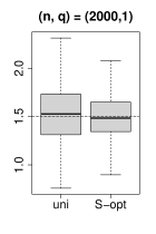
(a)

(b)

(c)

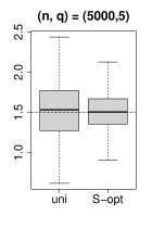
(d)

Figure 1: Boxplots for the ATE estimation with different combinations of $n$ and $q$; dashed lines are the true values.

Figure 1 shows that the efficiency of the ATE estimator is improved under $\tilde{\rho}_{\rm S}$ compared to the uniform rule. The improvement is consistently observed across different combinations of $n$ and $p$. We compute the relative efficiency (RE) under $\tilde{\rho}_{\rm S}$ with respect to the uniform rule. The RE of a sampling rule is the variance ratio of the estimator under the uniform rule to that under the considered sampling rule. Higher RE indicates greater improvement than the uniform rule. The REs are $1.6995$, $2.1835$, $1.8907$ and $2.3239$ for $(n,q)=(2000,1),(2000,5),(5000,1)$, and $(5000,5)$, respectively, which indicates significant efficiency improvements across different scenarios.

In practice, there may be multiple treatments. In this case, the ATEs of different treatments compared to the control are of interest. Next, we consider the ATE estimation with two different treatments (denoted by “$1$”, and “$2$”) and a control group (denoted by “$0$”). Define $Z$ in the same way as in the scalar case. Suppose $X$ follows the model

$$X=\zeta_{q}^{{\mathrm{\scriptscriptstyle T}}}Z+\epsilon_{x},$$

where $\epsilon_{x}$ follows a normal distribution with mean zero and variance $0.25$. The potential outcomes are generated from

$$Y_{0}=0.5\zeta_{q}^{{\mathrm{\scriptscriptstyle T}}}Z+X+\{0.5+\nu_{2}(Z)\}\epsilon_{y},$$

$$Y_{1}=\theta_{01}+0.5\zeta_{q}^{{\mathrm{\scriptscriptstyle T}}}Z-X+\{\nu_{1}(Z)+\nu_{2}(Z)\}\epsilon_{y},$$

$$Y_{2}=\theta_{02}-0.5\zeta_{q}^{{\mathrm{\scriptscriptstyle T}}}Z-0.5X+\nu_{2}(Z)\epsilon_{y},$$

where $\theta_{01}=1$, $\theta_{02}=0.5$, $\epsilon_{y}$ follows a standard normal distribution, $\nu_{1}(z)=\sqrt{0.1+(2\zeta_{q}^{{\mathrm{\scriptscriptstyle T}}}z)^{4}}$, and $\nu_{2}(z)=\exp(2\zeta_{q}^{{\mathrm{\scriptscriptstyle T}}}z)$. It is easy to verify that the ATEs $E[Y_{1}-Y_{0}]$ and $E[Y_{2}-Y_{0}]$ equal to $\theta_{01}$ and $\theta_{02}$, respectively. Suppose the treatment indicator $T$ equals to $0$, $1$, and $2$ with probabilities $1-p_{1}(X,Z)-p_{2}(X,Z)$, $p_{1}(X,Z)$ and $p_{2}(X,Z)$, where

$$p_{1}(X,Z) =\frac{\exp(-0.1\zeta_{q}^{{\mathrm{\scriptscriptstyle T}}}Z+0.25X)}{1+\exp(-0.1\zeta_{q}^{{\mathrm{\scriptscriptstyle T}}}Z+0.25X)+\exp(0.1\zeta_{q}^{{\mathrm{\scriptscriptstyle T}}}Z-0.25X)},$$

$$p_{2}(X,Z) =\frac{\exp(0.1\zeta_{q}^{{\mathrm{\scriptscriptstyle T}}}Z-0.25X)}{1+\exp(-0.1\zeta_{q}^{{\mathrm{\scriptscriptstyle T}}}Z+0.25X)+\exp(0.1\zeta_{q}^{{\mathrm{\scriptscriptstyle T}}}Z-0.25X)}.$$

The observed outcome $Y$ equals to $Y_{t}$ if $T=t$ for $t=0,1,$ and $2$.

Table 1 presents the bias, standard error (SE) of the estimator, and the RE compared to the uniform rule based on $500$ simulations.

Table 1: Bias, SE, and RE in two-dimensional ATE estimation

$(n,q)$	Rule	Estimate of $\theta_{01}$			Estimate of $\theta_{02}$
		Bias	SE	RE	Bias	SE	RE
$(2000,1)$	uni	-0.0047	0.5621	1.0000	0.0159	0.4742	1.0000
	C-opt	0.0050	0.4639	1.4680	0.0150	0.3609	1.7270
	G-opt	0.0103	0.4626	1.4765	0.0227	0.3502	1.8337
$(2000,5)$	uni	-0.0089	0.9309	1.0000	-0.0579	0.8495	1.0000
	C-opt	-0.0178	0.7629	1.4891	-0.0444	0.6420	1.7507
	G-opt	-0.0164	0.7385	1.5890	-0.0312	0.6161	1.9013
$(5000,1)$	uni	0.0208	0.3358	1.0000	-0.0006	0.2755	1.0000
	C-opt	0.0247	0.2585	1.6872	0.0027	0.2074	1.7652
	G-opt	0.0217	0.2482	1.8297	0.0010	0.2013	1.8732
$(5000,5)$	uni	-0.0117	0.5022	1.0000	-0.0013	0.4376	1.0000
	C-opt	-0.0181	0.4052	1.5359	-0.0218	0.3362	1.6945
	G-opt	0.0086	0.3942	1.6227	-0.0191	0.3055	2.0526

Table 1 shows that the standard errors are smaller under the sampling rules $\tilde{\rho}_{\rm C}$ and $\tilde{\rho}_{\rm G}$ than under the uniform rule. Moreover, the improvement is consistent and significant across different parameter components and values of $(n,q)$. In some cases, the RE is close to or even larger than two. The improvement of $\tilde{\rho}_{\rm G}$ tends to be greater than $\tilde{\rho}_{\rm C}$ in most cases, probably because $\tilde{\rho}_{\rm G}$ estimates the optimal solution over the full space, while $\tilde{\rho}_{\rm C}$ estimates the optimal solution over only a subspace. In addition, the simulation results in this section indicate that the proposed method’s performance remains stable even as the dimension of the first-phase variable increases. This suggests that the proposed method is not highly sensitive to the dimensionality of the first-phase variable despite the involvement of nonparametric methods in the estimation procedure.

6 Real Data Analysis

In this section, we illustrate the proposed approach using AIDS Clinical Trials Group (ACTG) 175 data (Hammer et al., 1996). The data used in this section can be found in the R package speff2trial. The ACTG175 clinical trial evaluates four therapies for treating human immunodeficiency virus infection. The four treatments are: $1$, zidovudine; $2$, zidovudine and didanosine; $3$, zidovudine and zalcitabine; and $4$, didanosine. In the trial, $2139$ subjects were assigned randomly to the four treatment groups. Covariates such as age, gender, weight, medication history, and symptom indicator were recorded before the treatment, and CD4 and CD8 cell counts were measured after $20$ weeks of the treatment. The CD4/CD8 ratio describes the overall immune function of an individual. A low value of CD4/CD8 ratio indicates a severe immune dysfunction. We use the CD4/CD8 ratio as the outcome variable and consider the ATE of the three zidovudine-treated groups (groups $1$, $2$, and $3$) compared to the non-zidovudine-treated group (group $4$). Let $\theta_{0j}$ be the ATE of the treatment $j$ compared to the treatment $4$ for $j=1,\dots,3$.

The original experiment measured CD4 and CD8 cell counts for all $2139$ subjects after $20$ weeks of the treatment. However, it can be costly to measure the CD4 and CD8 cell counts for more than two thousand people. The cost of the trials would be drastically reduced if a two-phase design were adopted and the CD4 and CD8 cell counts were measured for only a subset of patients. We applied the proposed method to design the second-phase sampling rule and obtained results as if the experiment was conducted under the two-phase design. We use six variables as the first-phase variables $V$, including age, gender, weight, medication history, symptom indicator, and treatment assignment. The outcome is considered as the second-phase variable $U$. In the implementation, we take $\varpi=0.3$ and $\kappa_{n}=\varpi/[1+\log(0.1n\varpi)]$. A pilot sample is randomly drawn with inclusion probability $\kappa_{n}$. The sampling rules $\tilde{\rho}_{\rm C}$ and $\tilde{\rho}_{\rm G}$ are constructed based on the pilot sample and the full data efficient influence function in Example 1 in Section A.1 of the Appendix. Then, a sample is drawn according to the resulting sampling rule. The full data efficient influence function involves the propensity score and the outcome regression function of each group. The propensity score for each group is $1/4$ because subjects were randomly assigned to each group with equal probability. We adopt a linear model for the outcome regression function.

We employ the one-step estimation method to estimate the ATEs using data drawn in the two phases. In line with the simulation, we use ”uni,” ”C-opt,” and ”G-opt” to represent the uniform rule, the sampling rule $\tilde{\rho}_{\rm C}$, and the sampling rule $\tilde{\rho}_{\rm G}$, respectively. Table 2 provides the estimates for $\theta_{01}$, $\theta_{02}$, and $\theta_{03}$ under different sampling rules. Additionally, it includes the estimated SEs based on the asymptotic variance of the estimator and p-values associated with the Wald tests for testing whether each ATE equals to zero.

Table 2: Point estimates (Est), estimated SEs, and p-values associated with the estimation of $\theta_{01}$, $\theta_{02}$, and $\theta_{03}$ in the ACTG175 trial under different sampling rules

Rule	Estimation of $\theta_{01}$			Estimation of $\theta_{02}$			Estimation of $\theta_{03}$
	Est	SE	p-value	Est	SE	p-value	Est	SE	p-value
uni	-0.0489	0.0223	0.0283	0.0166	0.0247	0.5013	-0.0034	0.0228	0.8805
C-opt	-0.0592	0.0212	0.0052	0.0191	0.0234	0.4151	-0.0010	0.0216	0.9640
G-opt	-0.0649	0.0210	0.0020	0.0169	0.0232	0.4661	0.0000	0.0215	0.9999

Table 2 shows that the estimators for $\theta_{01}$, $\theta_{02}$, and $\theta_{03}$ all have smaller estimated SEs under $\tilde{\rho}_{\rm C}$ and $\tilde{\rho}_{\rm G}$ compared to the uniform rule. The p-values under $\tilde{\rho}_{\rm C}$ and $\tilde{\rho}_{\rm G}$ suggest that, at the $0.01$ significance level, treatment $1$ performs differently than treatment $4$ in increasing the CD4/CD8 ratio, while there is no significant difference between treatments $2$, $3$, and treatment $4$. In contrast, the results under the uniform rule discover no significant difference among treatments $1$, $2$, $3$, and treatment $4$ under the significance level $0.01$. For comparison, we calculate the augmented inverse probability weighted (AIPW) estimator for $\theta_{01}$, $\theta_{02}$, and $\theta_{03}$ based on the first-phase variables and the outcome of all subjects. It is worth noting that the AIPW estimator requires measuring the outcome of all $2139$ subjects, while it only needs to measure the outcome of approximately $30\%$ of the subjects to obtain the estimates in Table 2. The all data-based estimates are $-0.0500$, $0.0166$, and $0.0054$ for $\theta_{01}$, $\theta_{02}$ and $\theta_{03}$, respectively, with p-values $0.0005$, $0.2851$, and $0.7140$. These p-values support the same conclusions as those suggested by the estimators under $\tilde{\rho}_{\rm C}$ and $\tilde{\rho}_{\rm G}$.

7 Discussion

This paper introduces a unified framework for designing sampling rules in two-phase studies. The proposed method offers promising guarantees in terms of estimation efficiency and budget control. It exhibits broad applicability across diverse research domains, such as the electronic health record data analysis (Lotspeich et al., 2021; Zhang et al., 2020), genetic association analysis (Lin et al., 2013), causal inference (Lin and Chen, 2014; Yang and Ding, 2019), and measurement error problems. Our framework accommodates multi-dimensional parameters, making it well-suited for association studies involving multiple traits and the estimation of causal effects with multiple treatments. However, the current framework relies on the semiparametric efficiency bound for a parameter vector of a fixed dimension. Therefore, an important direction for future research is the development of suitable criteria for high-dimensional problems and the corresponding optimal designs.

Appendix

Appendix A Examples

A.1 Examples of full data efficient influence function

Example 2.

Let $Y$ be a vector of outcomes which is hard to obtain. Suppose the parameter of interest is the outcome mean $\theta_{0}=E[Y]$. Let $Z$ be a vector of inexpensive covariates that is predictive to $Y$ and hence useful in estimating $\theta_{0}$. In two-phase studies, one can collect $V=Z$ in the first phase and measure $U=Y$ for a subset of subjects in the second phase. In this example, the full data efficient influence function is $\psi=Y-\theta_{0}$.

Example 3.

Let $Y$ be a scalar outcome which is easy to obtain, $Z$ a vector of inexpensive covariates, and $X$ a vector of expensive covariates. Suppose the parameter of interest is the least squares regression coefficient $\theta_{0}$ of $X$ in the regression of $Y$ on $Z,X$, which is determined by the estimating equation $E[(X^{{\mathrm{\scriptscriptstyle T}}},Z^{{\mathrm{\scriptscriptstyle T}}})^{{\mathrm{\scriptscriptstyle T}}}(Y-X^{{\mathrm{\scriptscriptstyle T}}}\theta_{0}-Z^{{\mathrm{\scriptscriptstyle T}}}\beta_{0})]=0$ where $\beta_{0}$ is the nuisance parameter. In two-phase studies, $V=(Y,Z)$ is collected in the first phase and $U=X$ is measured for a subset of subjects in the second phase. In this case, the full data efficient influence function is $\psi=(E[(X-\alpha_{0}Z)(X-\alpha_{0}Z)^{{\mathrm{\scriptscriptstyle T}}}])^{-1}(X-\alpha_{0}Z)(Y-X^{{\mathrm{\scriptscriptstyle T}}}\theta_{0}-Z^{{\mathrm{\scriptscriptstyle T}}}\beta_{0})$ where $\alpha_{0}=E[XZ^{{\mathrm{\scriptscriptstyle T}}}](E[ZZ^{{\mathrm{\scriptscriptstyle T}}}])^{-1}$ is the population linear regression coefficient of $X$ on $Z$.

The outcome mean estimation in Example 2 is an important problem in survey sampling (Cochran, 2007) and epidemiological studies (McNamee, 2002; Gilbert et al., 2014). Regression problems with expensive covariates in Example 3 are of great interest in modern epidemiological and clinical studies (Zeng and Lin, 2014; Zhou et al., 2014; Tao et al., 2017), because the determination of a disease’s risk factor can often boil down to such a regression problem.

A.2 Example for the Issue with a Multi-dimensional Parameter

Example 4.

Suppose $Y\in\{0,1\}$ is an indicator of some disease status and $X\in\{0,1\}$ is the test result of some fallible test for disease status. Suppose $V=X$ and $U=Y$. The prevalence of the disease $\theta_{01}=P(Y=1)$, sensitivity $\theta_{02}=P(X=1\mid Y=1)$ and specificity $\theta_{03}=P(X=0\mid Y=0)$ of the test are often of primary interest in epidemiological studies. Let $\theta_{0}=(\theta_{01},\theta_{02},\theta_{03})^{{\mathrm{\scriptscriptstyle T}}}$ be the parameter of interest. It is not hard to show the efficient influence functions of $\theta_{01}$, $\theta_{02}$ and $\theta_{03}$ are $Y-\theta_{01}$, $\theta_{01}^{-1}(X-\theta_{02})Y$ and $(1-\theta_{01})^{-1}(1-X-\theta_{03})(1-Y)$, respectively. Let $P(X)=P(Y=1\mid X)$. The conditional variances $\sigma_{1}^{2}(V)$, $\sigma_{2}^{2}(V)$ and $\sigma_{3}^{2}(V)$ are $P(X)(1-P(X))$, $\theta_{01}^{-2}P(X)(1-P(X))(X-\theta_{02})^{2}$ and $(1-\theta_{01})^{-2}P(X)(1-P(X))(1-X-\theta_{03})^{2}$, which are different from each other. According to Theorem 1, the optimal sampling rule for $\theta_{0j}$ is determined by $\sigma_{j}^{2}(\cdot)$. This implies that the optimal sampling rules for different parameters are different from each other. Hence, there is no sampling rule that minimizes the semiparametric efficiency bound for different parameters simultaneously in general.

Suppose $\theta_{01}=0.2$, $\theta_{02}=0.8$, $\theta_{03}=0.6$ and $\varpi=0.3$. Then some numerical calculations can show that the semiparametric efficiency bound for $\theta_{03}$ under $\rho_{\rm sum}(\cdot;\tau_{\rm sum})$ and the optimal sampling rule for $\theta_{01}$ are approximately $0.35$ and $0.43$, which are both larger than that under the uniform rule ($\approx 0.30$).

Appendix B Technical Details

B.1 Regularity Conditions

Let $F_{0}$ be the distribution of $(V,U)$. We consider the case where the parameter of interest is a general functional of $F_{0}$. Throughout this paper, we assume $\rho(\cdot)$ is bounded away from zero and $E[\|\psi\|^{2}]<\infty$ where $\|\cdot\|$ denotes the Euclidean norm.

As in Newey (1994), we consider inference of a pathwise differentiable parameter within a locally nonparametric distribution class. Here we briefly review the definitions of “pathwise differentiable” and “locally nonparametric”. See Bickel (1982); van der Laan and Robins (2012); Tsiatis (2007) for more background on semiparametric theory. Let $\mathcal{F}$ be a set of joint distributions of $(V,U)$ whose specific definition depends on the problem we consider. Suppose $F_{0}\in\mathcal{F}$. A class of distributions $\{F_{\lambda}:\lambda\in[-1,1]\}$ is called a submodel of $\mathcal{F}$ if it is contained in $\mathcal{F}$ and the distribution $F_{\lambda}$ equals to $F_{0}$ when $\lambda=0$. Suppose $F_{\lambda}$ has a density $f_{\lambda}(v,u)$ and let $S(v,u)=d\log f_{\lambda}(v,u)/d\lambda\big{|}_{\lambda=0}$ be the score function under the submodel. Suppose the parameter $\theta_{0}=\theta(F_{0})$ is a functional of $F_{0}$ where $\theta(\cdot)$ is a functional defined on $\mathcal{F}$. Then the parameter is pathwise differentiable if there is some function $\phi(V,U)$ with zero mean and finite variance such that $d\theta(F_{\lambda})/d\lambda\big{|}_{\lambda=0}=E[\phi(V,U)S(V,U)]$ for any regular submodel.

Pathwise differentiability is a commonly used regularity condition in semiparametric theory (Bickel, 1982). Here, a regular submodel is a submodel that satisfies certain regularity conditions. See Bickel (1982) for more discussions and the formal definition of a regular submodel. Typical examples of pathwise differentiable parameters including the mean or quantile of a variable, the solution of many commonly used estimating equations among lots of other parameters.

“Locally nonparametric” is a property of the distribution class $\mathcal{F}$. Because all the submodels are required to belong to $\mathcal{F}$, the fewer the restrictions on $\mathcal{F}$, the more submodels, and hence the larger the set of score functions. Here, “locally nonparametric” requires $\mathcal{F}$ to be “general” or “unrestricted” in the sense that the set of score functions can approximate any function of $(V,U)$ with zero mean and finite variance. In a locally nonparametric distribution class, general misspecification is allowed and few restrictions are imposed except for regularity conditions (Newey, 1994). For example, the distribution class which consists of all the distributions with a finite second moment is a locally nonparametric distribution class. For a missing data problem, all the observation distributions with response missing at random also consists of a locally nonparametric class.

B.2 Proof of Lemma 1

This lemma can be obtained from the results in Tsiatis (2007) and Li and Luedtke (2021). To be self-contained, we provide its proof here.

Proof.

We show the efficient influence function is

$$h=\frac{R\psi}{\rho(V)}-\left(\frac{R}{\rho(V)}-1\right)\Pi(V)$$

and the semiparametric efficiency bound follows by straightforward calculation. The observed likelihood of $(U,V,R)$ is

$$f(u\mid v)^{r}f(v)\rho(v)^{r}(1-\rho(v))^{1-r},$$

where $f(v)$ is the density of $V$ and $f(u\mid v)$ is the distribution of $U$ conditional on $V=v$. For any regular submodel $f_{\lambda}(u\mid v)f_{\lambda}(v)\rho(v)^{r}(1-\rho(v))^{1-r}$ whose distribution is denoted by $F_{\lambda}$, the score function is

$$rS(u\mid v)+S(v),$$ (10)

where

$$S(u\mid v)=\frac{d}{d\lambda}\log f_{\lambda}(u\mid v),$$

and

$$S(v)=\frac{d}{d\lambda}\log f_{\lambda}(v).$$

We do not consider a submodel for $\rho(v)$ since the sampling rule is determined by the researcher and hence is known in this problem. Because $\psi$ is the full data influence function and $E[S(U\mid V)\mid V]=0$, we have

$$\frac{d\theta(\lambda)}{d\lambda} =E[\psi S(U\mid V)]+E[\psi S(V))]$$ (11)

$$=E\left[hRS(U\mid V)\right]+E\left[hS(V)\right]$$

$$=E\left[h\{RS(U\mid V)+S(V)\}\right].$$

According to (10), the tangent space under the two-phase design consists of all functions of the form $rS(u\mid v)+S(v)$, where $S(u\mid v)$ and $S(v)$ are the score function of $f(u\mid v)$ and $f(v)$ under some full data submodel. Since the full data model is locally nonparametric, the closure of the tangent space under the two-phase design consists of all score functions of the form (10), which is

$$\mathcal{T}=\{rs(u,v)+s(v)\ :\ E[s(U,V)\mid V]=0,\ E[s(V)]=0\}.$$

It is easy to verify that $h$ belongs to $\mathcal{T}$. This and (11) implies $h$ is the efficient influence function according to the characterization of the efficient influence function which can be found behind Lemma 25.14 in van der Vaart (1998). ∎

B.3 Proof of Theorem 1

Proof.

Recall that $\rho_{\rm S}(\cdot)=\rho(\cdot;\sigma,\tau_{\rm S})$. By the definition of $\tau_{\rm S}$, the sampling rule $\rho_{\rm S}(\cdot)$ satisfies the constraint $E[\rho_{\rm S}(V)]=E[\rho(V;\sigma,\tau_{\rm S})]\leq\varpi$. Because the second term in the efficiency bound (2) is irrelevant to the sampling rule, to show $\rho(\cdot;\sigma,\tau_{\rm S})$ is the optimal sampling rule, it suffices to prove

$$E\left[\frac{\sigma^{2}(V)}{\rho^{\star}(V)}\right]\geq E\left[\frac{\sigma^{2}(V)}{\rho(V;\sigma,\tau_{\rm S})}\right]$$

for any sampling rule $\rho^{\star}(\cdot)$ satisfying $E[\rho^{\star}(V)]\leq\varpi$. Note that

$$E\left[\frac{\sigma^{2}(V)}{\rho^{\star}(V)}\right]-E\left[\frac{\sigma^{2}(V)}{\rho(V;\sigma,\tau_{\rm S})}\right] \geq E\left[\frac{\sigma^{2}(V)}{\rho^{2}(V;\sigma,\tau_{\rm S})}\left(\rho(V;\sigma,\tau_{\rm S})-\rho^{\star}(V)\right)\right]$$

$$=E\left[\sigma^{2}(V)\left(\rho(V;\sigma,\tau_{\rm S})-\rho^{\star}(V)\right)1\{\sigma(V)>\tau_{\rm S}\}\right]$$

$$\quad+\tau_{\rm S}^{2}E\left[\left(\rho(V;\sigma,\tau_{\rm S})-\rho^{\star}(V)\right)1\{\sigma(V)\leq\tau_{\rm S}\}\right]$$

$$\geq\tau_{\rm S}^{2}E\left[\rho(V;\sigma,\tau_{\rm S})-\rho^{\star}(V)\right]$$

$$=\tau_{\rm S}^{2}(\varpi-E\left[\rho^{\star}(V)\right])\geq 0,$$

where the first inequality is because $1/z_{1}-1/z_{2}\geq(z_{2}-z_{1})/z_{2}^{2}$ for any $z_{1}$, $z_{2}>0$. This completes the proof. ∎

B.4 Proof of Proposition 1

Proof.

Recall that $\mathcal{P}_{\rm G}\colonequals\{\rho(\cdot):0\leq\rho(\cdot)\leq 1,\ E[\rho(V)]\leq\varpi\}$ and $\mathcal{W}^{{\dagger}}=\{w=(w_{1},\dots,w_{d}):\sum_{j=1}^{d}w_{j}=1,\ 0\leq w_{j}\leq 1,\ \text{for}\ j=1,\dots,d\}$. Let

$$h(\rho,w)=\sum_{j=1}^{d}w_{j}\xi_{j}-E\left[\frac{\sum_{j=1}^{d}w_{j}\sigma_{j}^{2}(V)}{\rho(V)}\right].$$

Take the $L_{2}$ norm and the Euclidean norm as the norm in $\mathcal{P}$ and $\mathcal{W}^{{\dagger}}$, respectively. Then $\mathcal{P}$, $\mathcal{W}$ are compact and $h(\rho,w)$ is continuous with respect to $\rho$ and $q$. Moreover, $h(\rho,w)$ is convex with respect to $\rho$ and linear (hence concave) w.r.t. $w$. Thus the solution of the optimization problem does not change if we change the order of $\max$ and $\min$ in (6) according to Theorem 3.4 in Sion (1958). ∎

B.5 Proof of Theorem 2

Theorem 2 is obtained from Proposition 1 and the arguments before Theorem 2.

B.6 Proof of Theorem 3

Proof.

We prove the result for $\tilde{\rho}_{j}(\cdot)$ for $j=1,\dots,d$. The result for $\tilde{\rho}_{\rm C}(\cdot)$ and $\tilde{\rho}_{\rm G}(\cdot)$ can be established similarly. For $i=1,\dots,n$, the expectation of $R_{2i}$ is $(1-R_{1i})\tilde{\rho}_{j}(V_{i})$ conditional on $(R_{11},V_{1}),\dots,$ $(R_{1n},V_{n})$ and $U_{j}$ for $j$ with $R_{1j}=1$. Thus conditional on the same variables, the expectation of $\sum_{i=1}^{n}(R_{1i}+R_{2i})$ is $\sum_{i=1}^{n}R_{1i}+\sum_{i=1}^{n}(1-R_{1i})\tilde{\rho}_{j}(V_{i})$. Because $\tilde{\tau}_{j}$ is the solution of (9), we have $\sum_{i=1}^{n}(1-R_{1i})\tilde{\rho}_{j}(V_{i})=(\varpi-\kappa_{n})n$. According to the law of iterated conditional expectation, we have $E\left[\sum_{i=1}^{n}(R_{1i}+R_{2i})\right]=\kappa_{n}n+(\varpi-\kappa_{n})n=\varpi n$ which proves Theorem 3. ∎

B.7 Proof of Theorem 4

In this and the following proofs, we use $M$ to denote generic positive constants whose values may be different in different places. We first get down to the required regularity conditions.

Condition 2.

There is some constants $r_{j},L_{j}>0$ such that $\tau_{j}-r_{j}>0$ and $|E[\rho(V;\sigma_{j},\tau_{1})]-E[\rho(V;\sigma_{j},\tau_{2})]|>L_{j}|\tau_{1}-\tau_{2}|$ for any $\tau_{1},\tau_{2}\in[\tau_{j}-r_{j},\tau_{j}+r_{j}]$ and $j=1,\dots,d$, where $\rho(\cdot;\sigma_{j},\tau)=1\{\sigma_{j}(V)>\tau\}+\sigma_{j}(V)/\tau 1\{\sigma_{j}(V)\leq\tau\}$.

Condition 3.

$0<\inf_{v}\sigma_{j}(v)\leq\sup_{v}\sigma_{j}(v)<\infty$ for $j=1,\dots,d$.

Condition 2 requires that the budgets under different thresholds are different in a neighborhood of $\tau_{j}$. Condition 3 is a mild regularity condition. Next, we give the proof of Theorem 4.

Proof.

We prove the results for $\tilde{\rho}_{j}(\cdot)$ for $j=1,\dots,d$. The result for $\tilde{\rho}_{\rm S}(\cdot)$ is a special case of $d=1$.

We first show $\tilde{\tau}_{j}$ converges to $\tau_{j}$ for $j=1,\dots,d$, where $\tilde{\tau}_{j}$ is the solution of Equation (9) in the main text. Let $\tau_{{j},n}$ be the solution of $E[\rho(V;\sigma_{j},\tau)]=(\varpi-\kappa_{n})/(1-\kappa_{n})$. Note that $(\varpi-\kappa_{n})/(1-\kappa_{n})-\varpi=O(\kappa_{n})$. Under Condition 2, we have $|\tau_{{j},n}-\tau_{j}|=O(\kappa_{n})$. Next, we show that $|\tilde{\tau}_{j}-\tau_{{j},n}|$ converges to zero. For $\tau\in[\tau_{j}-r_{j},\tau_{j}+r_{j}]$, define

$$h_{{j},n}(\tau)=\frac{1}{n}\sum_{i=1}^{n}(1-R_{1i})\left(1\{\sigma(V_{i})\geq\tau\}+\frac{\sigma_{j}(V_{i})}{\tau}1\{\sigma_{j}(V_{i})<\tau\}\right)$$

and

$$\tilde{h}_{{j},n}(\tau)=\frac{1}{n}\sum_{i=1}^{n}(1-R_{1i})\left(1\{\tilde{\sigma}_{j}(V_{i})\geq\tau\}+\frac{\tilde{\sigma}_{j}(V_{i})}{\tau}1\{\tilde{\sigma}_{j}(V_{i})<\tau\}\right).$$

By calculating the mean and variance, we have

$$|h_{{j},n}(\tau)-E[h_{{j},n}(\tau)]|=O_{P}\left(\frac{1}{\sqrt{n}}\right)$$ (12)

uniformly in $\tau\in[\tau_{j}-r_{j},\tau_{j}+r_{j}]$. Moreover, we have $E[h_{{j},n}(\tau)]=(1-\kappa_{n})E[\rho(V;\sigma_{j},\tau)]$ which implies $E[h_{{j},n}(\tau)]=\varpi-\kappa_{n}$. By Condition 1, it is not hard to verify

$$|\tilde{h}_{{j},n}(\tau)-h_{{j},n}(\tau)|\leq\frac{1}{\tau_{j}-r}\|\tilde{\sigma}-\sigma\|_{\infty}=O_{P}\left\{(n\kappa_{n})^{-\delta}\right\}$$ (13)

uniformly in $\tau\in[\tau_{j}-r_{j},\tau_{j}+r_{j}]$, where $\delta$ is a constant determined by the convergence rate of $\|\tilde{\sigma}_{j}-\sigma_{j}\|_{\infty}$ which appears in Condition 1 . Combining (12) and (13), we have

$$|\tilde{h}_{{j},n}(\tau)-E[h_{{j},n}(\tau)]|=O_{P}\left\{(n\kappa_{n})^{-\delta}\right\}.$$

Thus for any $\epsilon>0$, there is some constant $M>0$ such that

$$P\left(|\tilde{h}_{{j},n}(\tau)-E[h_{j,n}(\tau)]|\geq M(n\kappa_{n})^{-\delta}\right)\leq\frac{\epsilon}{2}$$

for any $\tau\in[\tau_{j}-r_{j},\tau_{j}+r_{j}]$. Define $\tau_{{j},n,1}=\tau_{{j},n}-M(n\kappa_{n})^{-\delta}/(L_{j}(1-\kappa_{n}))$ and $\tau_{{j},n,2}=\tau_{{j},n}+M(n\kappa_{n})^{-\delta}/(L_{j}(1-\kappa_{n}))$. Because $|\tau_{{j},n}-\tau_{j}|=O(\kappa_{n})$, $\kappa_{n}\to 0$ and $n\kappa_{n}\to\infty$, we have $\tau_{{j},n}$, $\tau_{{j},n,1}$, $\tau_{{j},n,2}\in[\tau_{j}-r_{j},\tau_{j}+r_{j}]$ for sufficiently large $n$. Hence

$$P\Big{(}\tilde{h}_{{j},n}(\tau_{{j},n,1})-E[h_{{j},n}(\tau_{{j},n,1})]<M(n\kappa_{n})^{-\delta},\tilde{h}_{{j},n}(\tau_{{j},n,2})-E[h_{{j},n}(\tau_{{j},n,2})]>-M(n\kappa_{n})^{-\delta}\Big{)}$$ (14)

$$\geq 1-P\left(\tilde{h}_{{j},n}(\tau_{{j},n,1})-E[h_{{j},n}(\tau_{{j},n,1})]\geq M(n\kappa_{n})^{-\delta}\right)$$

$$\quad-P\left(\tilde{h}_{{j},n}(\tau_{{j},n,2})-E[h_{{j},n}(\tau_{{j},n,2})]\leq-M(n\kappa_{n})^{-\delta}\right)$$

$$\geq 1-\epsilon$$

for sufficiently large $n$. According to Condition 2 and the monotonicity of $E[h_{{j},n}(\tau)]=(1-\kappa_{n})E[\rho(V;\sigma_{j},\tau)]$, we have

$$E[h_{{j},n}(\tau_{{j},n,1})]\leq\varpi-\kappa_{n}-M(n\kappa_{n})^{-\delta}$$

and

$$E[h_{{j},n}(\tau_{{j},n,2})]\geq\varpi-\kappa_{n}+M(n\kappa_{n})^{-\delta}.$$

Combining this with (14), we have

$$P\left(\tilde{h}_{{j},n}(\tau_{{j},n,1})<\varpi-\kappa_{n}<\tilde{h}_{{j},n}(\tau_{{j},n,2})\right)\geq 1-\epsilon.$$

Recall that $\tilde{\tau}_{j}$ is the solution of $\tilde{h}_{j,n}(\tau)=\varpi-\kappa_{n}$. By the monotonicity of $\tilde{h}_{{j},n}(\tau)$, we have $P\left(\tilde{\tau}_{j}\in[\tau_{{j},n,1},\tau_{{j},n,2}]\right)\geq 1-\epsilon$. This implies $|\tilde{\tau}_{j}-\tau_{{j},n}|=O_{P}\{(n\kappa_{n})^{-\delta}\}$ and hence

$$|\tilde{\tau}_{j}-\tau_{j}|=O_{P}\{(n\kappa_{n})^{-\delta}+\kappa_{n}\}.$$ (15)

Under Condition 3, we have

$$|\tilde{\rho}_{j}(v)-\rho_{j}(v)|$$

$$=\left|1\{\tilde{\sigma}_{j}(v)>\tilde{\tau}_{j}\}+\frac{\tilde{\sigma}_{j}(v)}{\tilde{\tau}_{j}}1\{\tilde{\sigma}_{j}(v)\leq\tilde{\tau}_{j}\}-1\{\sigma_{j}(v)>\tau_{j}\}-\frac{\sigma_{j}(v)}{\tau_{j}}1\{\sigma_{j}(v)\leq\tau_{j}\}\right|$$

$$\leq\left|1\{\tilde{\sigma}_{j}(v)>\tilde{\tau}_{j}\}+\frac{\tilde{\sigma}_{j}(v)}{\tilde{\tau}_{j}}1\{\tilde{\sigma}_{j}(v)\leq\tilde{\tau}_{j}\}-1\{\sigma_{j}(v)>\tilde{\tau}_{j}\}-\frac{\sigma_{j}(v)}{\tilde{\tau}_{j}}1\{\sigma_{j}(v)\leq\tilde{\tau}_{j}\}\right|$$

$$+\left|1\{\sigma_{j}(v)>\tilde{\tau}_{j}\}+\frac{\sigma_{j}(v)}{\tilde{\tau}_{j}}1\{\sigma_{j}(v)\leq\tilde{\tau}_{j}\}-1\{\sigma_{j}(v)>\tau_{j}\}-\frac{\sigma_{j}(v)}{\tau_{j}}1\{\sigma_{j}(v)\leq\tau_{j}\}\right|$$

$$\leq M(\|\tilde{\sigma}_{j}-\sigma_{j}\|_{\infty}+|\tilde{\tau}_{j}-\tau_{j}|)$$

for some constant $M$ with probability approaching one. Combining this with Condition 1 and Equation (15), we have

$$\|\tilde{\rho}_{j}-\rho_{j}\|_{\infty}=O_{P}\left\{(n\kappa_{n})^{-\delta}+\kappa_{n}\right\},$$

which completes the proof. ∎

B.8 Proof of Theorem 5

In this subsection, we turn to the convergence result of the estimated sampling rule in the multi-dimensional parameter case. For $w\in\mathcal{W}$, define

$$H_{j}(w)=-\xi_{j}+E\left[\frac{\sigma_{j}^{2}(V)}{\rho_{0}(V)+\sum_{j=1}^{d}w_{j}(\rho_{j}(V)-\rho_{0}(V_{i}))}\right]$$

and

$$H_{\rm C}(w)=\max_{j=1,\dots,d}H_{j}(w),$$

where $\xi_{j}=E[\sigma_{j}^{2}(V)/\rho_{0}(V)]$ for $j=1,\dots,d$. Similarly, for $w\in\mathcal{W}^{\star}$, let

$$H_{\rm G}(w)=\sum_{j=1}^{d}w_{j}\xi_{j}-E\left[\sigma_{w}(V)\max\{\sigma_{w}(V),\tau_{w}\}\right].$$

Then $w_{\rm C}=\mathop{\arg\min}_{w\in\mathcal{W}}H_{\rm C}(w)$ and $w_{\rm G}=\mathop{\arg\min}_{w\in\mathcal{W}^{{\dagger}}}H_{\rm G}(w)$. The following condition is required to establish the convergence rate of $\tilde{\rho}_{\rm C}(\cdot)$ and $\tilde{\rho}_{\rm G}(\cdot)$.

Condition 4.

The benchmark sampling rule $\rho_{0}(\cdot)$ is bounded away from zero and satisfies $E[\rho_{0}(V)]=\varpi$.

Condition 5.

(i) $H_{\rm C}(w)$ has the unique minimum point $w_{\rm C}$; (ii) for some constants $r_{\rm C},L_{\rm C}>0$ and any $w\in\mathcal{W}$ such that $\|w-w_{\rm C}\|\leq r_{\rm C}$, we have $H_{\rm C}(w)-H_{\rm C}(w_{\rm C})\geq L_{\rm C}\|w-w_{\rm C}\|^{2}$.

Condition 6.

(i) $H_{\rm G}(w)$ has the unique minimum point $w_{\rm G}$; (ii) for some constants $r_{\rm G},L_{\rm G}>0$ and any $w\in\mathcal{W}^{{\dagger}}$ such that $\|w-w_{\rm G}\|\leq r_{\rm G}$, we have $H_{\rm G}(w)-H_{\rm G}(w_{\rm G})\geq L_{\rm G}\|w-w_{\rm G}\|^{2}$.

Condition 4 is a regularity condition on the benchmark sampling rule $\rho_{0}(\cdot)$. Condition 5 is a mild regularity condition, which can be satisfied if $H_{\rm C}(w)$ has a continuous Hessian matrix in a neighborhood of $r_{\rm C}$ and the Hessian matrix at $r_{\rm C}$ is positive definite. Condition 6 is similar to Condition 5 with $H_{\rm C}(w)$ replaced by $H_{\rm G}(w)$. Now, we are ready to prove Theorem 5.

Proof.

We only prove the result for $\tilde{\rho}_{\rm C}(\cdot)$. The result for $\tilde{\rho}_{\rm G}(\cdot)$ can be established similarly.

Recall that $\rho_{\rm C}(\cdot)=\rho_{0}(\cdot)+\sum_{j=1}^{d}w_{{\rm C},j}\{\rho_{j}(\cdot)-\rho_{0}(\cdot)\}$ and $\tilde{\rho}_{\rm C}(\cdot)=\rho_{0}(\cdot)+\sum_{j=1}^{d}\widetilde{w}_{{\rm C},j}(\tilde{\rho}_{j}(\cdot)-\rho_{0}(\cdot))$, where $w_{{\rm C},j}$ and $\widetilde{w}_{{\rm C},j}$ are the $j$th component of $w_{\rm C}$ and $\widetilde{w}_{\rm C}$, respectively, for $j=1,\dots,d$. Recall that $\rho_{j}(v)=1\{\sigma_{j}(v)>\tau_{j}\}+\sigma_{j}(v)1\{\sigma_{j}(v)\leq\tau_{j}\}/\tau_{j}$ for $j=1,\dots,d$. By Condition 3, we have

$$\frac{1}{M}\leq\inf_{v}\rho_{j}(v)\leq\sup_{v}\rho_{j}(v)\leq M$$ (16)

for some $M>1$. Hence

$$\|\tilde{\rho}_{\rm C}-\rho_{\rm C}\|_{\infty}\leq\sum_{j=1}^{d}\|\tilde{\rho}_{j}-\rho_{j}\|_{\infty}+M\|\tilde{w}_{\rm C}-w_{\rm C}\|.$$

Theorem 4 has established the convergence rate of $\|\tilde{\rho}_{j}-\rho_{j}\|_{\infty}$. Thus, in order to establish the convergence rate of $\|\tilde{\rho}_{\rm C}-\rho_{\rm C}\|_{\infty}$, it suffices to establish the convergence rate of $\|\widetilde{w}_{\rm C}-w_{\rm C}\|$ . Define

$$\widetilde{H}_{j}(w)=-\tilde{\xi}_{j}+\frac{1}{n}\sum_{i=1}^{n}\frac{\tilde{\sigma}_{j}^{2}(V)}{\rho_{0}(V)+\sum_{j=1}^{d}w_{j}(\tilde{\rho}_{j}(V)-\rho_{0}(V_{i}))}$$

and

$$\widetilde{H}_{\rm C}(w)=\max_{j=1,\dots,d}\widetilde{H}_{j}(w),$$

where $\tilde{\xi}_{j}=n^{-1}\sum_{i=1}^{n}\tilde{\sigma}_{j}^{2}(V_{i})/\rho_{0}(V_{i})$ for $j=1,\dots,d$. Then $\widetilde{w}_{\rm C}=\mathop{\arg\min}_{w\in\mathcal{W}}\widetilde{H}_{\rm C}(w)$. Define $\bar{H}_{j}(w)$ similarly to $\widetilde{H}_{j}(w)$ with $\tilde{\sigma}_{j}(\cdot)$ and $\tilde{\rho}_{j}(\cdot)$ in $\widetilde{H}_{j}(w)$ replaced by $\sigma_{j}(\cdot)$ and $\rho_{j}(\cdot)$. Let $\bar{H}_{\rm C}(w)=\max_{j=1,\dots,d}\bar{H}_{j}(w)$. According to Condition 1, Theorem 4, and inequality (16), there is some constant $M>1$ such that $1/M\leq\inf_{v}\tilde{\rho}_{j}(v)\leq\sup_{v}\tilde{\rho}_{j}(v)\leq M$ with probability approaching one. Then, Condition 4 and the mean value theorem implies that there is some constant $M$ such that

$$\sup_{w\in\mathcal{W}}|\widetilde{H}_{j}(w)-\bar{H}_{j}(w)|\leq M(\|\tilde{\sigma}_{j}-\sigma_{j}\|_{\infty}+\|\tilde{\rho}_{j}-\rho_{j}\|_{\infty})$$

with probability approaching one. This implies

$$\sup_{w\in\mathcal{W}}|\widetilde{H}_{\rm C}(w)-\bar{H}_{\rm C}(w)|\leq M\left(\max_{j=1,\dots,d}\|\tilde{\sigma}_{j}-\sigma_{j}\|_{\infty}+\max_{j=1,\dots,d}\|\tilde{\rho}_{j}-\rho_{j}\|_{\infty}\right)$$

with probability approaching one. Then, according to Condition 1 and Theorem 4, we have

$$\sup_{w\in\mathcal{W}}|\widetilde{H}_{\rm C}(w)-\bar{H}_{\rm C}(w)|=O_{P}\left\{(n\kappa_{n})^{-\delta}+\kappa_{n}\right\}.$$ (17)

Recall that

$$\bar{H}_{j}(w)=\frac{1}{n}\sum_{i=1}^{n}\left\{-\frac{\sigma_{j}^{2}(V_{i})}{\rho_{0}(V_{i})}+\frac{\sigma_{j}^{2}(V_{i})}{\rho_{0}(V_{i})+\sum_{j=1}^{d}w_{j}(\rho_{j}(V_{i})-\rho_{0}(V_{i}))}\right\}$$

for any $w\in\mathcal{W}$. Straightforward calculation can show that $E[\bar{H}_{j}(w)]=H_{j}(w)$. Notice that the function $\sigma_{j}(v)/\rho_{0}(v)+\sigma_{j}(v)/[\rho_{0}(v)+\sum_{j=1}^{d}w_{j}(\rho_{j}(v)-\rho_{0}(v))]$ is bounded and Lipschitz continuous with respect to $w$ due to (16), Condition 3, and Condition 4. Then, similar arguments as in the proof of Lemma C.1 in He et al. (2021) can show that

$$\sup_{w\in\mathcal{W}}|\bar{H}_{j}(w)-H_{j}(w)|=O_{P}\left(\frac{1}{\sqrt{n}}\right).$$ (18)

Combining (17) with (18), we have

$$\sup_{w\in\mathcal{W}}|\widetilde{H}_{j}(w)-H_{j}(w)|=O_{P}\left\{(n\kappa_{n})^{-\delta}+\kappa_{n}\right\}.$$

Thus, for any $\epsilon>0$, there is some $M>0$ such that $P(\sup_{w\in\mathcal{W}}|\widetilde{H}_{j}(w)-H_{j}(w)|\geq M\{(n\kappa_{n})^{-\delta}+\kappa_{n}\})\leq\epsilon$. Because $\widetilde{w}_{\rm C}$ is the minimum point of $\widetilde{H}_{\rm C}(w)$, we have $\widetilde{H}_{\rm C}(\widetilde{w}_{\rm C})\leq\widetilde{H}_{\rm C}(w_{\rm C})$ and hence

$$H_{\rm C}(\widetilde{w}_{\rm C})-H_{\rm C}(w_{\rm C}) \leq\widetilde{H}_{\rm C}(\widetilde{w}_{\rm C})-\widetilde{H}_{\rm C}(w_{\rm C})+2\sup_{w\in\mathcal{W}}|\widetilde{H}_{j}(w)-H_{j}(w)|$$

$$\leq 2\sup_{w\in\mathcal{W}}|\widetilde{H}_{j}(w)-H_{j}(w)|.$$

Thus

$$H_{\rm C}(\widetilde{w}_{\rm C})-H_{\rm C}(w_{\rm C})\leq 2M\{(n\kappa_{n})^{-\delta}+\kappa_{n}\}$$ (19)

with probability at least $1-\epsilon$. Because $H_{\rm C}(w)$ is continuous with respect to $w$, $\mathcal{W}$ is a compact set and $w_{\rm C}$ is the unique minimum point of $H_{\rm C}(w)$, we have $\inf_{w\in\mathcal{W},\|w-w_{\rm C}\|\geq r_{\rm C}}\{H_{\rm C}(w)-H_{\rm C}(w_{\rm C})\}>0$ for $r_{\rm C}$ in Condition 5. For sufficiently large $n$ such that $2M\{(n\kappa_{n})^{-\delta}+\kappa_{n}\}<\inf_{w\in\mathcal{W},\|w-w_{\rm C}\|\geq r_{\rm C}}\{H_{\rm C}(w)-H_{\rm C}(w_{\rm C})\}$, we have $\|\widetilde{w}_{\rm C}-w_{\rm C}\|\leq r_{\rm C}$ with probability at least $1-\epsilon$ according to (19). Then inequality (19) and Condition 5 imply $\|\widetilde{w}_{\rm C}-w_{\rm C}\|\leq\sqrt{2M\{(n\kappa_{n})^{-\delta}+\kappa_{n}\}/L_{\rm C}}$ with probability at least $1-\epsilon$. Because $\epsilon$ is arbitrary, we have $\|\widetilde{w}_{\rm C}-w_{\rm C}\|=O_{P}(\sqrt{(n\kappa_{n})^{-\delta}+\kappa_{n}})$. Combining this with Condition 3 and the fact that $\|\tilde{\rho}_{j}-\rho_{j}\|_{\infty}=O_{P}\{(n\kappa_{n})^{-\delta}+\kappa_{n}\}$, we conclude that $\|\tilde{\rho}_{\rm C}-\rho_{\rm C}\|_{\infty}=O_{P}(\sqrt{(n\kappa_{n})^{-\delta}+\kappa_{n}})$. ∎

Appendix C Estimation

C.1 Estimate the Conditional Mean and Variance of the Efficient Influence Function

The full data efficient influence function depends on $\theta_{0}$ and may also depend on some unknown nuisance parameters, e.g., $\alpha_{0}$ and $\beta_{0}$ in Example 3 and $m_{1}(\cdot)$, $m_{0}(\cdot)$ and $\pi(\cdot)$ in Example 1. Thus, we need to estimate these unknown quantities. We write the efficient influence function as $\psi(V,U;\theta_{0},\eta_{0})$ where $\eta_{0}$ is the nuisance parameter. The nuisance parameter $\eta_{0}$ can be estimated using the pilot sample. Denote the resulting estimator by $\tilde{\eta}$. Then $\theta_{0}$ can be estimated by $\tilde{\theta}$ which is the solution of the estimating equation

$$\sum_{i=1}^{n}R_{1i}\psi(V_{i},U_{i};\theta,\tilde{\eta})=0,$$

where $R_{1i}$ is the inclusion indicator for the pilot sample. Then we obtain the estimates $\tilde{\psi}_{i}=\psi(V_{i},U_{i};\tilde{\theta},\tilde{\eta})$ ($i:R_{1i}=1$) for the full data efficient influence function of observations in the pilot sample.

In order to estimate the optimal sampling rule and construct efficient estimator according to the efficient influence function in Lemma 1, one needs to estimate the conditional mean $\Pi_{j}(\cdot)$ and the standard deviation $\sigma_{j}(\cdot)$ for $j=1,\dots,d$. These quantities can be estimated by fitting a heteroscedastic parametric regression model using the pilot sample and the estimated $\tilde{\psi}_{i}$’s. In practice, it may be hard to model $\Pi_{j}(\cdot)$ and $\sigma_{j}(\cdot)$ for $j=1,\dots,d$. If plausible parametric models are not available, we recommend to estimate them nonparametrically. Many methods are available for this task, including kernel smoothing (Fan and Yao, 1998; Fan and Gijbels, 2018), sieve methods (Huang, 1998, 2001; Chen, 2007) and kernel ridge regression (Mendelson, 2002). A sieve method that can estimate the conditional mean and standard deviation simultaneously is proposed in the next section. The proposed method is computationally efficient and performs well even when the dimension of the first-phase variable is moderately high.

C.2 New Nonparametric Estimators for the Conditional Mean and Variance

If a plausible model for the conditional mean function $\Pi_{j}(v)$ is unavailable for $j=1,\dots,d$, we can approximate it with a linear combination of some basis functions such as polynomials, wavelets, or splines. Let $p(v)=(p_{1}(v),\dots,p_{K}(v))^{{\mathrm{\scriptscriptstyle T}}}$ be a vector of basis functions which changes with $n$. In particular, we let $K$ increase with $n$ to make the approximation more and more accurate as the sample size increases. Then we approximate $\Pi_{j}(v)$ by $\gamma_{1}^{{\mathrm{\scriptscriptstyle T}}}p(v)$ for some $\gamma_{1}$. The conditional standard deviation $\sigma_{j}(v)$ can be approximate similarly by $\gamma_{2}^{{\mathrm{\scriptscriptstyle T}}}p(v)$ for some $\gamma_{2}$. However, this approximation is not guaranteed to be non-negative. An infeasible negative sampling rule is obtained if we plug the negative approximation into the expression of the optimal sampling rule in Theorem 1. Using the truncated version $\max\{\gamma_{2}^{{\mathrm{\scriptscriptstyle T}}}p(v),0\}$ can avoid this problem but leads the function not differentiable with respect to $\gamma_{2}$ which makes optimization difficult. Hence we propose to use a transformation function $\Lambda(v)=\log(1+\exp(v))$ and use $\Lambda(\gamma_{2}^{{\mathrm{\scriptscriptstyle T}}}p(v))$ to approximate $\sigma_{j}(v)$. The function $\Lambda(v)$ is a smooth approximation of the truncation function $\max\{v,0\}$. Moreover, it is convex, Lipchitz continuous, differentiable, and non-negative. These nice properties benefit the optimization.

Then, the remaining problem is to determine $\gamma_{1}$ and $\gamma_{2}$. The discussion behind Theorem 1 can show that $\sigma_{j}(\cdot)$ minimizes $E[(\psi_{j}-\Pi_{j}(V))^{2}/f_{2}(V)]$ over all positive $f_{2}(\cdot)$ such that $E[f_{2}(V)]\leq E[\sigma_{j}(V)]$. This motivates us to consider the penalized objective formulation of the constrained optimization problem $E[(\psi_{j}-\Pi_{j}(V))^{2}/f_{2}(V)]+E[f_{2}(V)]$. One can verify that this objective function is minimized if $f_{2}(\cdot)=\sigma_{j}(\cdot)$. On the other hand, it is straightforward to show, for any given positive function $f_{2}(\cdot)$, the conditional mean function $\Pi_{j}(\cdot)$ minimizes the weighted least squares objective function $E[(\psi_{j}-f_{1}(V))^{2}/f_{2}(V)]+E[f_{2}(V)]$ over all $f_{1}(\cdot)$. This inspires us to recover the conditional mean and variance simultaneously by minimizing $E[(\psi_{j}-f_{1}(V))^{2}/f_{2}(V)]+E[f_{2}(V)]$ with respect to $f_{1}(\cdot)$ and $f_{2}(\cdot)$. By replacing the expectation with sample mean and plugging in the estimates and approximations, we obtain the objective function

$$\mathcal{L}_{nj}(\gamma_{1},\gamma_{2})=\frac{1}{n\kappa_{n}}\sum_{i=1}^{n}R_{1i}\left\{\frac{(\tilde{\psi}_{ij}-\gamma_{1}^{{\mathrm{\scriptscriptstyle T}}}p(V_{i}))^{2}}{\Lambda(\gamma_{2}^{{\mathrm{\scriptscriptstyle T}}}p(V_{i}))}+\Lambda(\gamma_{2}^{{\mathrm{\scriptscriptstyle T}}}p(V_{i}))\right\},$$ (20)

where $\tilde{\psi}_{ij}$ is the $j$th component of $\tilde{\psi}_{i}$ for $j=1,\dots,d$ and $i=1,\dots,n$. Let $\tilde{\gamma}_{1j},$ $\tilde{\gamma}_{2j}$ be the minimum point of (20). Then $\Pi_{j}(V)$ and $\sigma_{j}(V)$ can be estimated by $\widetilde{\Pi}_{j}(V)=\tilde{\gamma}_{1j}^{{\mathrm{\scriptscriptstyle T}}}p(V)$ and $\tilde{\sigma}_{j}(V)=\Lambda(\tilde{\gamma}_{2j}^{{\mathrm{\scriptscriptstyle T}}}p(V))$, respectively. The proposed objective function has the following block-wise convex property.

Proposition 2.

For $j=1,\dots,d$ and any give $\gamma_{1}$, $\mathcal{L}_{nj}(\gamma_{1},\gamma_{2})$ is convex with respect to $\gamma_{2}$; for $j=1,\dots,d$ and any give $\gamma_{2}$, $\mathcal{L}_{nj}(\gamma_{1},\gamma_{2})$ is convex with respect to $\gamma_{1}$.

Proof.

For any given $\gamma_{1}$, the Hessian of $\mathcal{L}_{nj}(\gamma_{1},\gamma_{2})$ with respect to $\gamma_{2}$ is

$$\frac{1}{n\kappa_{n}}\sum_{i=1}^{n}R_{1i}p(V_{i})p(V_{i})^{{\mathrm{\scriptscriptstyle T}}}\Big{\{}(\tilde{\psi}_{i}-\gamma_{1}^{{\mathrm{\scriptscriptstyle T}}}p(V_{i}))^{2}\left[2\Lambda(\gamma_{2}^{{\mathrm{\scriptscriptstyle T}}}p(V_{i}))^{-3}\Lambda^{(1)}(V_{i})^{2}-\Lambda(\gamma_{2}^{{\mathrm{\scriptscriptstyle T}}}p(V_{i}))^{-2}\Lambda^{(2)}(V_{i})^{2}\right]$$

$$\qquad\qquad+\Lambda^{(2)}(\gamma_{2}^{{\mathrm{\scriptscriptstyle T}}}p(V_{i}))\Big{\}}$$

where $\Lambda^{(1)}(v)=\exp(v)/\{1+\exp(v)\}$ and $\Lambda^{(2)}(v)=\exp(v)/\{1+\exp(v)\}^{2}$. This matrix is positive semi-definite because $\Lambda^{(2)}(v)>0$ and $2\Lambda(v)^{-3}\Lambda^{(1)}(v)^{2}-\Lambda(v)^{-2}\Lambda^{(2)}(v)>0$. Thus $\mathcal{L}_{nj}(\gamma_{1},\gamma_{2})$ is convex with respect to $\gamma_{2}$. For any given $\gamma_{2}$, the Hessian of $\mathcal{L}_{nj}(\gamma_{1},\gamma_{2})$ with respect to $\gamma_{1}$ is

$$\frac{1}{n\kappa_{n}}\sum_{i=1}^{n}R_{1i}p(V_{i})p(V_{i})^{{\mathrm{\scriptscriptstyle T}}}\frac{2}{\Lambda(\gamma_{2}^{{\mathrm{\scriptscriptstyle T}}}p(V_{i}))},$$

which is also positive semi-definite. This completes the proof. ∎

Proposition 2 shows $\mathcal{L}_{nj}(\gamma_{1},\gamma_{2})$ is block-wise convex with respect to $\gamma_{1}$ and $\gamma_{2}$ for $j=1,\dots,d$ and hence the optimization problem (20) can be solved efficiently by routine optimization algorithms. So far we have defined a nonparametric estimator for $\Pi_{j}(V)$, $\sigma_{j}(V)$ based on the sieve method (Chen, 2007). For our numerical experiments, the estimators $\widetilde{\Pi}_{j}$ and $\tilde{\sigma}_{j}$ are employed. During the simulation, we introduce a small regularization $0.1(d_{V}+1)(\|\gamma_{1}\|^{2}+\|\gamma_{2}\|^{2})$ into the loss function (20) to further enhance the stability of the solution, where $d_{V}$ is the dimension of the first-phase variable $V$.

The idea to recover the mean and variance simultaneously also appears in parametric heterogeneous regression literature and is shown to perform well in finite sample (Daye et al., 2012; Spady and Stouli, 2018). Our estimator is an extension of the idea to the nonparametric literature. The proposed method has several nice properties compared to other nonparametric conditional mean and variance estimators, such as kernel smoothing, sieve least squares, and kernel ridge regression. First, it is computationally efficient as the conditional mean and variance can be estimated simultaneously by solving the optimization problem (20). Second, heteroscedasticity is considered in fitting the conditional mean model, which can deliver efficiency gains when fitting a model with many parameters and limited observations (Daye et al., 2012). Third, the conditional variance estimator is always positive. This is also a desirable property (Yu and Jones, 2004) which is not possessed by some classic existing methods, e.g., local linear kernel smoothing, sieve least squares, and kernel ridge regression.

C.3 Estimate the Parameters of Interest

Define $R_{2i}=0$ for subjects with $R_{1i}=1$. With some abuse of notation, let $R_{i}=R_{1i}+R_{2i}$ be the overall sampling indicator for the second phase sampling. Under the sampling procedure proposed in Section C, $V_{i}$ is measured for all the $n$ subjects, and $U_{i}$ is measured for subjects with $R_{i}=1$. If a nonrandom sampling rule $\rho(\cdot)$ is used to select the subsequent sample in the second phase, we have the inclusion probability $P(R_{i}=1\mid V_{i})=\kappa_{n}+(1-\kappa_{n})\rho(V_{i})$ for $i=1,\dots,n$. Denote the sampling rule adopted in the second phase by $\tilde{\rho}(\cdot)$, where $\tilde{\rho}(\cdot)$ depends on the pilot sample and hence is random. However, it converges to some nonrandom sampling rule according to Theorem 5. Thus the inclusion probability can be approximated by $\rho_{n}(V_{i})=\kappa_{n}+(1-\kappa_{n})\tilde{\rho}(V_{i})$. Let the inverse probability weighted estimator $\hat{\theta}_{\rm ipw}$ be the solution of the estimating equation

$$\sum_{i=1}^{n}\frac{R_{i}\psi(V_{i},U_{i};\theta,\tilde{\eta})}{\rho_{n}(V_{i})}=0.$$

The inverse probability weighted estimator $\hat{\theta}_{\rm ipw}$ is $\sqrt{n}$-consistent under certain regularity conditions but may not be efficient (Tsiatis, 2007). Based on $\hat{\theta}_{\rm ipw}$, an efficient estimator can be obtained through one-step estimation (Bickel, 1982). Let $\widetilde{\Pi}(\cdot)$ be an estimate of $\Pi(\cdot)$ based on the pilot sample. According to the efficient influence function given in Lemma 1, the one-step estimator is defined by

$$\hat{\theta} =\hat{\theta}_{\rm ipw}+\sum_{i=1}^{n}\frac{R_{i}\psi(V_{i},U_{i};\hat{\theta}_{\rm ipw},\tilde{\eta})}{\rho_{n}(V_{i})}-\sum_{i=1}^{n}\left(\frac{R_{i}}{\rho_{n}(V_{i})}-1\right)\widetilde{\Pi}(V_{i})$$

$$=\hat{\theta}_{\rm ipw}-\sum_{i=1}^{n}\left(\frac{R_{i}}{\rho_{n}(V_{i})}-1\right)\widetilde{\Pi}(V_{i}),$$

The one-step estimator $\hat{\theta}$ is asymptotically normal and efficient under appropriate empirical process conditions (van der Laan and Robins, 2012; van der Vaart and Wellner, 1996).

Appendix D Additional Simulations

D.1 Response Mean

In this section, we consider the response mean estimation problem where covariates are inexpensive and the response is hard to obtain. As in the main text, we set $n=5000$. Let $Z$ be a $q$-dimensional covariate vector with independent $U[-2.5,2.5]$ components, where $U[-2.5,2.5]$ is the uniform distribution on $[-2.5,2.5]$. Suppose the response

$$Y=\theta_{0}+\zeta_{q}^{{\mathrm{\scriptscriptstyle T}}}Z+\nu_{1}(Z)\epsilon,$$

where $\theta_{0}=1$, $\zeta_{q}=(0.5/\sqrt{q},\dots,0.5/\sqrt{q})^{{\mathrm{\scriptscriptstyle T}}}$, $\nu_{1}(z)=\sqrt{0.1+(2\zeta_{q}^{{\mathrm{\scriptscriptstyle T}}}z)^{4}}$, $\epsilon$ is the standard normal error. In this example, we let $V=Z$ be the vector of first-phase variables and $U=Y$ be the second-phase variable. The parameter of interest is the response mean $\theta_{0}=E[Y]$. Figure 2 is the boxplot based on the results of $500$ simulations.

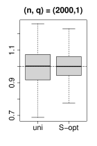
(a)

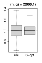
(b)

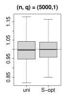
(c)

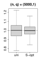
(d)

Figure 2: Boxplots for the mean estimation with different combinations of $n$ and $q$; dashed lines are the true values.

As can be seen in Fig. 2, the estimation efficiency is improved under $\tilde{\rho}_{\rm S}$ compared to the uniform rule. The improvement is observed for different combinations of $n$ and $q$, and is particularly pronounced when $q=5$. The REs are $1.5038$, $1.7409$, $1.5103$, and $2.1777$ when $(n,q)=(2000,1),(2000,5),(5000,1)$, and $(5000,5)$, which indicates that the efficiency is significantly improved under the proposed optimal sampling rule compared to that under the uniform rule.

In the following, we consider the problem of multi-dimensional parameter estimation and evaluate the effectiveness of the sampling rule $\tilde{\rho}_{\rm C}$ and $\tilde{\rho}_{\rm G}$. We consider a two-dimensional response variable $Y=(Y_{1},Y_{2})^{{\mathrm{\scriptscriptstyle T}}}$. Suppose

$$Y_{1}=\theta_{01}-\zeta_{q}^{{\mathrm{\scriptscriptstyle T}}}Z+\nu_{1}(Z)\epsilon_{1},$$

$$Y_{2}=\theta_{02}+\sin(\zeta_{q}^{{\mathrm{\scriptscriptstyle T}}}Z)+\nu_{2}(Z)\epsilon_{2},$$

where $\theta_{01}=1$, $\theta_{02}=0$, $\nu_{1}(z)$ is introduced in the scalar case, $\nu_{2}(z)=\exp(2\zeta_{q}^{{\mathrm{\scriptscriptstyle T}}}z)$, $\epsilon_{1}$ and $\epsilon_{2}$ are independent standard normal errors, and $Z$ is defined in the same way as in the scalar case. We consider the estimation of the two-dimensional response mean $\theta_{0}=(\theta_{01},\theta_{02})^{{\mathrm{\scriptscriptstyle T}}}=(E[Y_{1}],E[Y_{2}])^{{\mathrm{\scriptscriptstyle T}}}$ under two-phase designs. Table 3 reports the bias and standard error (SE) of the one-step estimator with different sampling rules based on $500$ simulations, and the RE compared to the uniform rule.

Table 3: Bias, SE, and RE in two-dimensional mean estimation

$(n,q)$	Rule	Estimate of $\theta_{01}$			Estimate of $\theta_{02}$
		Bias	SE	RE	Bias	SE	RE
$(2000,1)$	uni	0.0017	0.1224	1.0000	-0.0012	0.1601	1.0000
	C-opt	-0.0021	0.0922	1.7634	-0.0007	0.1225	1.7075
	G-opt	-0.0017	0.0950	1.6586	0.0058	0.1254	1.6291
$(2000,5)$	uni	-0.0001	0.1541	1.0000	0.0216	0.2494	1.0000
	C-opt	0.0037	0.1023	2.2714	0.0026	0.1549	2.5923
	G-opt	0.0093	0.1024	2.2674	0.0108	0.1549	2.5913
$(5000,1)$	uni	0.0008	0.0719	1.0000	0.0047	0.0981	1.0000
	C-opt	-0.0024	0.0584	1.5171	0.0018	0.0762	1.6581
	G-opt	0.0001	0.0578	1.5487	-0.0011	0.0749	1.7150
$(5000,5)$	uni	-0.0012	0.0854	1.0000	-0.0032	0.1591	1.0000
	C-opt	-0.0004	0.0632	1.8246	-0.0023	0.1004	2.5122
	G-opt	-0.0009	0.0587	2.1213	0.0015	0.1031	2.3824

In all cases, the SEs under the sampling rules $\tilde{\rho}_{\rm C}$ and $\tilde{\rho}_{\rm G}$ are smaller than that under the uniform rule. In some cases, the improvement is very significant with a RE larger than $2.5$.

D.2 Linear Regression Coefficient

In this subsection, we consider the problem of estimating linear regression coefficients when response variables and a part of covariates are measured in the first phase and other covariates are measured in the second phase. Define $Z$ in the same way as in Section D.1. Suppose

$$X=\sin(\zeta_{q}^{{\mathrm{\scriptscriptstyle T}}}Z)+\nu_{2}(Z)\epsilon_{x},$$

$$Y=\zeta_{q}^{{\mathrm{\scriptscriptstyle T}}}Z+\theta_{0}X+\epsilon_{y},$$

where $\theta_{0}=1$, $\nu_{2}(z)$ is defined in the last Section D.1, and $\epsilon_{x}$ and $\epsilon_{y}$ are independent and follow a standard normal distribution. Let $V=(Y,Z^{{\mathrm{\scriptscriptstyle T}}})^{{\mathrm{\scriptscriptstyle T}}}$ be the first-phase variable vector and $U=X$ be the second-phase variable. The estimation of the regression coefficient $\theta_{0}$ is considered in this simulation. Figure 3 contains boxplots of the estimator in $500$ simulations across different combinations of $n$ and $q$.

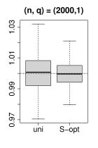
(a)

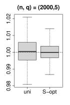
(b)

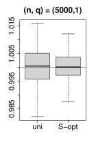
(c)

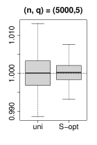
(d)

Figure 3: Boxplots for linear regression coefficient estimation with different combinations of $n$ and $q$; dashed lines are the true values.

As can be seen in Fig. 3, the accuracy of the estimator is improved under $\tilde{\rho}_{\rm S}$ compared to that under the uniform rule. The improvements are observed across different combinations of $n$ and $q$, and is particularly pronounced when $(n,q)=(5000,5)$. The REs are $2.1276$, $2.1387$, $2.1728$, and $2.493$ when $(n,q)=(2000,1),(2000,5),(5000,1)$, and $(5000,5)$.

Next, we consider the case with a two-dimensional regression coefficient of interest. The covariate vector $Z$ is defined in the same way as in Section D.1. Let $X=(X_{1},X_{2})^{{\mathrm{\scriptscriptstyle T}}}$ be a two-dimensional covariate vector which satisfies

$$X_{1}=\zeta_{q}^{{\mathrm{\scriptscriptstyle T}}}Z+\nu_{1}(Z)\epsilon_{x1},$$

$$X_{2}=-\zeta_{q}^{{\mathrm{\scriptscriptstyle T}}}Z+\nu_{2}(Z)\epsilon_{x2},$$

where $\nu_{1}(z)$ and $\nu_{2}(z)$ are defined in Section D.1, $\epsilon_{x1}$, $\epsilon_{x2}$ are independent standard normal variables. The response variable $Y$ satisfies

$$Y=\zeta_{q}^{{\mathrm{\scriptscriptstyle T}}}Z+\theta_{0}^{{\mathrm{\scriptscriptstyle T}}}X+\epsilon_{y},$$

where $\theta_{0}^{T}=(\theta_{01},\theta_{02})=(0,1)$ and $\epsilon_{y}$ follows a standard normal distribution.

Table 4 reports the bias, SE of the one-step estimator, and the RE compared to the uniform rule.

Table 4: Bias, SE, and RE in two-dimension regression coefficient estimation

$(n,q)$	Rule	Estimate of $\theta_{01}$			Estimate of $\theta_{02}$
		Bias	SE	RE	Bias	SE	RE
$(2000,1)$	uni	-0.0006	0.0151	1.0000	0.0015	0.0116	1.0000
	C-opt	-0.0013	0.0127	1.4164	0.0006	0.0092	1.5768
	G-opt	-0.0006	0.0128	1.4004	0.0006	0.0091	1.6201
$(2000,5)$	uni	-0.0003	0.0131	1.0000	0.0004	0.0076	1.0000
	C-opt	0.0003	0.0107	1.4995	0.0003	0.0059	1.6976
	G-opt	0.0004	0.0103	1.6332	0.0002	0.0054	1.9744
$(5000,1)$	uni	-0.0003	0.0095	1.0000	0.0003	0.0068	1.0000
	C-opt	-0.0002	0.0079	1.4777	0.0004	0.0054	1.6131
	G-opt	-0.0003	0.0082	1.3486	0.0001	0.0052	1.7338
$(5000,5)$	uni	0.0007	0.0080	1.0000	0.0002	0.0047	1.0000
	C-opt	-0.0001	0.0067	1.4297	0.0000	0.0030	2.4054
	G-opt	0.0004	0.0069	1.3486	-0.0001	0.0030	2.4564

As seen in Table 4, the SEs under under the sampling rules $\tilde{\rho}_{\rm C}$ and $\tilde{\rho}_{\rm G}$ are smaller than those under the uniform rule in all cases. The REs are larger than two in some cases.

References

- Bickel (1982) Bickel, P. J. (1982), “On adaptive estimation,” The Annals of Statistics, 647–671.
- Chen and Lumley (2020) Chen, T. and Lumley, T. (2020), “Optimal multiwave sampling for regression modeling in two-phase designs,” Statistics in Medicine, 39, 4912–4921.
- Chen and Lumley (2022) — (2022), “Optimal sampling for design-based estimators of regression models,” Statistics in Medicine, 41, 1482–1497.
- Chen (2007) Chen, X. (2007), “Large sample sieve estimation of semi-nonparametric models,” Handbook of Econometrics, 6, 5549–5632.
- Chen and Christensen (2015) Chen, X. and Christensen, T. M. (2015), “Optimal uniform convergence rates and asymptotic normality for series estimators under weak dependence and weak conditions,” Journal of Econometrics, 188, 447–465.
- Cochran (2007) Cochran, W. G. (2007), Sampling Techniques, John Wiley & Sons, 3rd ed.
- Daye et al. (2012) Daye, Z. J., Chen, J., and Li, H. (2012), “High-dimensional heteroscedastic regression with an application to eQTL data analysis,” Biometrics, 68, 316–326.
- Fan and Gijbels (2018) Fan, J. and Gijbels, I. (2018), Local polynomial modelling and its applications, Routledge.
- Fan and Yao (1998) Fan, J. and Yao, Q. (1998), “Efficient estimation of conditional variance functions in stochastic regression,” Biometrika, 85, 645–660.
- Gilbert et al. (2014) Gilbert, P. B., Yu, X., and Rotnitzky, A. (2014), “Optimal auxiliary-covariate-based two-phase sampling design for semiparametric efficient estimation of a mean or mean difference, with application to clinical trials,” Statistics in Medicine, 33, 901–917.
- Green et al. (1998) Green, D. M., Breslow, N. E., Beckwith, J. B., Finklestein, J. Z., Grundy, P. E., Thomas, P. R., Kim, T., Shochat, S. J., Haase, G. M., Ritchey, M. L., Kelalis, P. P., and D’Angio, G. J. (1998), “Comparison between single-dose and divided-dose administration of dactinomycin and doxorubicin for patients with Wilms’ tumor: a report from the National Wilms’ Tumor Study Group.” Journal of Clinical Oncology, 16, 237–245.
- Hammer et al. (1996) Hammer, S. M., Katzenstein, D. A., Hughes, M. D., Gundacker, H., Schooley, R. T., Haubrich, R. H., Henry, W. K., Lederman, M. M., Phair, J. P., Niu, M., Hirsch, M. S., and Merigan, T. C. (1996), “A trial comparing nucleoside monotherapy with combination therapy in hiv-infected adults with cd4 cell counts from 200 to 500 per cubic millimeter,” The New England Journal of Medicine, 335, 1081 – 1090.
- Hardle et al. (1988) Hardle, W., Janssen, P., and Serfling, R. (1988), “Strong uniform consistency rates for estimators of conditional functionals,” The Annals of Statistics, 1428–1449.
- He et al. (2021) He, X., Pan, X., Tan, K. M., and Zhou, W.-X. (2021), “Smoothed quantile regression with large-scale inference,” Journal of Econometrics.
- Huang (1998) Huang, J. Z. (1998), “Projection estimation in multiple regression with application to functional ANOVA models,” The Annals of Statistics, 26, 242–272.
- Huang (2001) — (2001), “Concave extended linear modeling: a theoretical synthesis,” Statistica Sinica, 173–197.
- Kiefer (1959) Kiefer, J. (1959), “Optimum experimental designs,” Journal of the Royal Statistical Society: Series B (Statistical Methodology), 21, 272–304.
- Li and Luedtke (2021) Li, S. and Luedtke, A. (2021), “Efficient estimation under data fusion,” arXiv:2111.14945.
- Lin et al. (2013) Lin, D.-Y., Zeng, D., and Tang, Z.-Z. (2013), “Quantitative trait analysis in sequencing studies under trait-dependent sampling,” Proceedings of the National Academy of Sciences, 110, 12247–12252.
- Lin and Chen (2014) Lin, H.-W. and Chen, Y.-H. (2014), “Adjustment for missing confounders in studies based on observational databases: 2-stage calibration combining propensity scores from primary and validation data,” American Journal of Epidemiology, 180, 308–317.
- Lotspeich et al. (2021) Lotspeich, S. C., Shepherd, B. E., Amorim, G. G., Shaw, P. A., and Tao, R. (2021), “Efficient odds ratio estimation under two-phase sampling using error-prone data from a multi-national HIV research cohort,” Biometrics.
- McGowan et al. (2007) McGowan, C. C., Cahn, P., Gotuzzo, E., Padgett, D., Pape, J. W., Wolff, M., Schechter, M., and Masys, D. R. (2007), “Cohort profile: Caribbean, Central and South America Network for HIV research (CCASAnet) collaboration within the international Epidemiologic databases to evaluate AIDS (IeDEA) programme,” International Journal of Epidemiology, 36, 969–976.
- McIsaac and Cook (2014) McIsaac, M. A. and Cook, R. J. (2014), “Response-dependent two-phase sampling designs for biomarker studies,” Canadian Journal of Statistics, 42, 268–284.
- McIsaac and Cook (2015) — (2015), “Adaptive sampling in two-phase designs: A biomarker study for progression in arthritis,” Statistics in Medicine, 34, 2899–2912.
- McNamee (2002) McNamee, R. (2002), “Optimal designs of two-stage studies for estimation of sensitivity, specificity and positive predictive value,” Statistics in Medicine, 21, 3609–3625.
- Mendelson (2002) Mendelson, S. (2002), “Geometric parameters of kernel machines,” in In Proceedings of the Fifteenth Annual Conference on Computational Learning Theory,, pp. 29–43.
- Newey (1994) Newey, W. K. (1994), “The asymptotic variance of semiparametric estimators,” Econometrica, 1349–1382.
- Reilly and Pepe (1995) Reilly, M. and Pepe, M. S. (1995), “A mean score method for missing and auxiliary covariate data in regression models,” Biometrika, 82, 299–314.
- Rigollet and Hütter (2015) Rigollet, P. and Hütter, J.-C. (2015), “High Dimensional Statistics,” Lecture Notes for Course 18S997, 813, 46.
- Sion (1958) Sion, M. (1958), “On general minimax theorems.” Pacific Journal of Mathematics, 8, 171–176.
- Spady and Stouli (2018) Spady, R. and Stouli, S. (2018), “Simultaneous mean-variance regression,” arXiv:1804.01631.
- Tao et al. (2017) Tao, R., Zeng, D., and Lin, D.-Y. (2017), “Efficient semiparametric inference under two-phase sampling, with applications to genetic association studies,” Journal of the American Statistical Association, 112, 1468–1476.
- Tao et al. (2020) — (2020), “Optimal designs of two-phase studies,” Journal of the American Statistical Association, 115, 1946–1959.
- Tsiatis (2007) Tsiatis, A. (2007), Semiparametric theory and missing data, Springer Science & Business Media.
- van der Laan and Robins (2012) van der Laan, M. J. and Robins, J. M. (2012), Unified Methods for Censored Longitudinal Data and Causality, Springer Science & Business Media.
- van der Laan and Rubin (2006) van der Laan, M. J. and Rubin, D. (2006), “Targeted maximum likelihood learning,” The International Journal of Biostatistics, 2.
- van der Vaart (1998) van der Vaart, A. W. (1998), Asymptotic Statistics, New York, NY: Cambridge University Press.
- van der Vaart and Wellner (1996) van der Vaart, A. W. and Wellner, J. A. (1996), Weak Convergence and Empirical Processes With Applications to Statistics, Springer, New York.
- White (1982) White, J. E. (1982), “A two stage design for the study of the relationship between a rare exposure and a rare disease,” American Journal of Epidemiology, 115, 119–128.
- Yang and Ding (2019) Yang, S. and Ding, P. (2019), “Combining multiple observational data sources to estimate causal effects,” Journal of the American Statistical Association.
- Yu and Jones (2004) Yu, K. and Jones, M. (2004), “Likelihood-based local linear estimation of the conditional variance function,” Journal of the American Statistical Association, 99, 139–144.
- Zeng and Lin (2014) Zeng, D. and Lin, D. (2014), “Efficient estimation of semiparametric transformation models for two-phase cohort studies,” Journal of the American Statistical Association, 109, 371–383.
- Zhang et al. (2020) Zhang, G., Beesley, L. J., Mukherjee, B., and Shi, X. (2020), “Patient Recruitment Using Electronic Health Records Under Selection Bias: a Two-phase Sampling Framework,” arXiv preprint arXiv:2011.06663.
- Zhou et al. (2014) Zhou, H., Xu, W., Zeng, D., and Cai, J. (2014), “Semiparametric inference for data with a continuous outcome from a two-phase probability-dependent sampling scheme,” Journal of the Royal Statistical Society: Series B (Statistical Methodology), 1, 197–215.