A fractional block-centered finite difference method for two-sided space-fractional diffusion equations on general nonuniform grids and its fast implementation

Abstract

In this paper, a two-sided variable-coefficient space-fractional diffusion equation with fractional Neumann boundary condition is considered. To conquer the weak singularity caused by the nonlocal space-fractional differential operators, by introducing an auxiliary fractional flux variable and using piecewise linear interpolations, a fractional block-centered finite difference (BCFD) method on general nonuniform grids is proposed. However, like other numerical methods, the proposed method still produces linear algebraic systems with unstructured dense coefficient matrices under the general nonuniform grids. Consequently, traditional direct solvers such as Gaussian elimination method shall require $\mathcal{O}(M^{2})$ memory and $\mathcal{O}(M^{3})$ computational work per time level, where $M$ is the number of spatial unknowns in the numerical discretization. To address this issue, we combine the well-known sum-of-exponentials (SOE) approximation technique with the fractional BCFD method to propose a fast version fractional BCFD algorithm. Based upon the Krylov subspace iterative methods, fast matrix-vector multiplications of the resulting coefficient matrices with any vector are developed, in which they can be implemented in only $\mathcal{O}(MN_{exp})$ operations per iteration, where $N_{exp}\ll M$ is the number of exponentials in the SOE approximation. Moreover, the coefficient matrices do not necessarily need to be generated explicitly, while they can be stored in $\mathcal{O}(MN_{exp})$ memory by only storing some coefficient vectors. Numerical experiments are provided to demonstrate the efficiency and accuracy of the method.

1 Introduction

Fractional partial differential equations provide a very adequate and competitive tool to model challenging phenomena involving anomalous diffusion or long-range memory and spatial interactions. For example, the space-fractional diffusion equations (SFDEs) can be used to describe the anomalous diffusion occurred in many transport processes [25, 3, 4, 34]. Extensive research has been conducted in the development of numerical methods for various fractional differential equations [35, 9, 24, 22, 14, 12, 27, 5, 11, 42, 21, 45, 33, 19, 6, 7, 32, 43]. However, due to the nonlocal nature of the fractional differential operators, numerical methods for SFDEs tend to generate dense and full stiffness matrices. Traditionally, these methods are solved via the direct solvers such as Gaussian elimination (GE) method, which requires a computational complexity of order $\mathcal{O}(M^{3})$ per time level and memory of order $\mathcal{O}(M^{2})$, where $M$ is the total number of spatial unknowns in the numerical discretization. Consequently, numerical simulations of SFDEs would lead to significantly increased memory requirement and computational complexity as $M$ increases. However, in the case of uniform spatial partitions, Toeplitz-like structure of the resulting stiffness matrices was discovered in [39] for space-fractional diffusion model, and thus based upon the special matrix structures, fast Krylov subspace iterative solvers are developed for different numerical methods of various SFDEs, in which both memory requirement and computational complexity have been largely reduced [36, 38, 10, 26, 47, 20, 12, 37].

On the other hand, it is shown that the solutions to SFDEs usually exhibit power function singularities near the boundary even under assumptions that the coefficients and right-hand side source term are sufficiently smooth [8, 18]. This motivates the usage of nonuniform grids to better capture the singular behavior of the solutions. Simmons [31] derived a first-order finite volume method on nonuniform grids for two-sided fractional diffusion equations. However, because the dense coefficient matrices do not have Toeplitz-like structure as the case of uniform grids, the previous developed fast algorithms will no longer be applicable. It makes sense to construct novel fast algorithms discretized on arbitrary nonuniform grids. Recently, finite volume methods based on special composite structured grids that consist of a uniform spatial partition far away the boundary and a locally refinement near the boundary were studied to address this issue [15, 5, 16], where Toeplitz-like structures of the coefficient matrices can be still found, and the Toeplitz structure of the diagonal blocks of the resulting block coefficient matrix was employed for efficient evaluate matrix-vector multiplications and the off-diagonal blocks were properly approximated by low-rank decompositions. As is known, fast approximations to the time-fractional diffusion equations have been extensively investigated [17, 46, 44]. However, there are still lack of fast numerical methods for SPDEs on general nonuniform grids. Recently, Jiang et al. [17] developed a novel sum-of-exponentials (SOE) technique for fast evaluation of the Caputo time-fractional derivative and applied to time-fractional diffusion equations. Then, by adopting the SOE technique on graded spatial grids, Fang et al. [11] proposed a fast first-order finite volume method for the one-dimensional SFDEs with homogeneous Dirichlet boundary condition. However, to our best knowledge, there seems currently few papers on construction of highly efficient numerical methods on general nonuniform spatial grids, which is still a major challenge for the modeling of SFDEs.

Block-centered finite difference (BCFD) method, sometimes called cell-centered finite difference method, can be thought of as the lowest-order Raviart-Thomas mixed element method, by employing a proper numerical quadrature formula [29]. One of the most important merits of the BCFD method is that it can simultaneously approximate the primal variable and its flux to a same order of accuracy on nonuniform grids, without any accuracy lost compared to the standard finite difference method. Besides, the BCFD method can very easily deal with model problems with Neumann or periodic boundary condition. In recent years, BCFD method has been widely used to simulate integer-order partial differential equations and time-fractional partial differential equations [30, 41, 23]. However, due to the complexity of the nonlocal space-fractional differential operators, we do not see any report of BCFD method for space-fractional partial differential equations. Therefore, we aim to present a fractional type BCFD method for model (1.1) with fractional Neumann boundary condition, in which nonuniform spatial grids are utilized to capture, for example, the boundary singularity of the solution and thus to improve the computational accuracy. Moreover, another main goal of this paper is to present a fast version fractional BCFD algorithm to accelerate the computational efficiency of modeling the SFDEs, in which a fast Krylov subspace iterative solver based upon efficient matrix-vector multiplications is developed.

The present paper focuses on efficient and accurate numerical approximation of the following two-sided variable-coefficient space-fractional diffusion equation with anomalous diffusion orders $1<\alpha,\beta<2$:

$$\partial_{t}u-\partial_{x}\,\mathcal{D}_{\gamma}^{x,\alpha}u(x,y,t) -\partial_{y}\,\mathcal{D}_{\theta}^{y,\beta}u(x,y,t)=f(x,y,t),$$ (1.1)

$$\qquad\quad(x,y)\in\Omega:=(a,b)\times(c,d),\quad 0<t\leq T,$$

where, $\mathcal{D}_{\gamma}^{x,\alpha}$ and $\mathcal{D}_{\theta}^{y,\beta}$ respectively represent the weighted fractional-order differential operators along $x$ and $y$ directions:

$$\mathcal{D}_{\gamma}^{x,\alpha} :=\gamma K^{x,L}\partial_{x}\,{}_{a}\mathcal{J}_{x}^{2-\alpha}+(1-\gamma)K^{x,R}\partial_{x}\,{}_{x}\mathcal{J}_{b}^{2-\alpha},$$

$$\mathcal{D}_{\theta}^{y,\beta} :=\theta K^{y,L}\partial_{y}\,{}_{c}\mathcal{J}_{y}^{2-\beta}+(1-\theta)K^{y,R}\partial_{y}\,{}_{y}\mathcal{J}_{d}^{2-\beta},$$

for weighted parameters $0\leq\gamma,\theta\leq 1$. The positive diffusion coefficients $K^{x,L}=K^{x,L}(x,y,t)$, $K^{x,R}=K^{x,R}(x,y,t)$, $K^{y,L}=K^{y,L}(x,y,t)$ and $K^{y,R}=K^{y,R}(x,y,t)$. Moreover, ${}_{a}\mathcal{J}_{x}^{2-\alpha}$, ${}_{x}\mathcal{J}_{b}^{2-\alpha}$, ${}_{c}\mathcal{J}_{y}^{2-\beta}$, and ${}_{y}\mathcal{J}_{d}^{2-\beta}$ respectively denote the following left-sided and right-sided Riemann-Liouville fractional integrals, defined by [28]

$${}_{a}\mathcal{J}_{x}^{\alpha}g(x,y):=\frac{1}{\Gamma(\alpha)}\int_{a}^{x}(x-s)^{\alpha-1}g(s,y)ds,\quad{}_{x}\mathcal{J}_{b}^{\alpha}g(x,y):=\frac{1}{\Gamma(\alpha)}\int_{x}^{b}(s-x)^{\alpha-1}g(s,y)ds,$$

$${}_{c}\mathcal{J}_{y}^{\beta}g(x,y):=\frac{1}{\Gamma(\beta)}\int_{c}^{y}(y-s)^{\beta-1}g(x,s)ds,\quad{}_{y}\mathcal{J}_{d}^{\beta}g(x,y):=\frac{1}{\Gamma(\beta)}\int_{y}^{d}(s-y)^{\beta-1}g(x,s)ds.$$

We assume that problem (1.1) is subjected to the following initial condition

$$u(x,y,0)=u^{o}(x,y),\quad\text{for}\quad(x,y)\in\bar{\Omega},$$ (1.2)

and fractional Neumann boundary conditions [40, 1]

$$\mathcal{D}_{\gamma}^{x,\alpha}u(x,y,t)\mid_{x=a}=\phi^{x}(y,t),\quad\mathcal{D}_{\gamma}^{x,\alpha}u(x,y,t)\mid_{x=b}=\varphi^{x}(y,t),$$ (1.3)

$$\mathcal{D}_{\theta}^{y,\beta}u(x,y,t)\mid_{y=c}=\phi^{y}(x,t),\quad\mathcal{D}_{\theta}^{y,\beta}u(x,y,t)\mid_{y=d}=\varphi^{y}(x,t).$$

In this paper, we first develop a fractional CN-BCFD method on general nonuniform grids for SFDEs (1.1)–(1.3) in one space dimension, in which a Crank-Nicolson (CN) temporal discretization combined with a fractional BCFD method in spatial discretization is developed by introducing an auxiliary fractional flux variable. Then, we develop fast approximation techniques to the left/right-sided Riemann-Liouville fractional integrals, using efficient SOE approximations to the kernels $x^{1-\alpha}$, $y^{1-\beta}$ ($\alpha,\beta\in(1,2)$) and piecewise linear interpolations of the primal variable $u$. Based upon these approximations, fast Krylov subspace iterative solvers for the fractional BCFD method is then proposed with fast matrix-vector multiplications of the resulting coefficient matrices with any vector. It is shown that the solver requires only $\mathcal{O}(MN_{exp})$ operations per iteration with efficient matrix storage mechanism, where $N_{exp}\ll M$ is the number of exponentials in the SOE approximation. Finally, ample numerical experiments are provided to demonstrate the efficiency and accuracy of the method. As far as we know, this seems to be the first time a fractional BCFD method and its efficient implementation are developed for the SFDEs, where fractional Neumann boundary condition is considered and general nonuniform spatial grids are adopted.

The rest of the paper is organized as follows. In Section 2, we present the fractional CN-BCFD method on nonuniform spatial grids for the SFDEs. In Section 3, a fast version fractional CN-BCFD method is proposed to further accelerate the computational efficiency. Then, we give some numerical experiments to investigate accuracy of the methods as well as performance of the fast method in Section 4. Some concluding remarks are given in the last section.

2 A fractional CN-BCFD method on general nonuniform grids

For simplicity of presentation, in this paper we pay our attention to the one-dimensional version of (1.1):

$$\left\{\begin{aligned} {}&\partial_{t}u-\partial_{x}\left(\gamma K^{x,L}\partial_{x}\,{}_{a}\mathcal{J}_{x}^{2-\alpha}u+(1-\gamma)K^{x,R}\partial_{x}\,{}_{x}\mathcal{J}_{b}^{2-\alpha}u\right)=f(x,t),~{}~{}a<x<b,\ 0<t\leq T,\\ &\left(\gamma K^{x,L}(x,t)\,\partial_{x}\,{}_{a}\mathcal{J}_{x}^{2-\alpha}u(x,t)+(1-\gamma)K^{x,R}(x,t)\,\partial_{x}\,{}_{x}\mathcal{J}_{b}^{2-\alpha}u(x,t)\right)\big{|}_{x=a}=\phi^{x}(t),~{}~{}0\leq t\leq T,\\ &\left(\gamma K^{x,L}(x,t)\,\partial_{x}\,{}_{a}\mathcal{J}_{x}^{2-\alpha}u(x,t)+(1-\gamma)K^{x,R}(x,t)\,\partial_{x}\,{}_{x}\mathcal{J}_{b}^{2-\alpha}u(x,t)\right)\big{|}_{x=b}=\varphi^{x}(t),~{}~{}0\leq t\leq T,\\ &u(x,0)=u^{o}(x),\quad a\leq x\leq b.\end{aligned}\right.$$ (2.1)

While, the extension to the two-dimensional case is straightforward but more complicated.

In the following, we introduce some notations. First, for a positive integer $N$, let $0=t_{0}<t_{1}<\cdots<t_{N}=T$ be a given sequence with uniform temporal stepsize $\tau:=T/N$. For temporal grid function $\left\{\Phi^{n}\right\}_{n=0}^{N}$, define

$$\Phi^{n-1/2}:=\frac{\Phi^{n}+\Phi^{n-1}}{2},\quad\delta_{t}\Phi^{n}:=\frac{\Phi^{n}-\Phi^{n-1}}{\tau}.$$

Next, for a positive integer $M$, define a set of nonuniform spatial grids by

$$a=x_{1/2}<x_{3/2}<\cdots<x_{M-1/2}<x_{M+1/2}=b,$$

with grid size $h_{i}=x_{i+1/2}-x_{i-1/2}$ for $i=1,2,\dots,M$ and $h:=\max_{1\leq i\leq M}h_{i}$. Besides, set $x_{i}:=\left(x_{i+1/2}+x_{i-1/2}\right)/2$ for $i=1,2,\ldots,M$, we thus define another set of nonuniform staggered spatial grids. Denote $h_{1/2}:=x_{1}-a=h_{1}/2$, $h_{i+1/2}:=x_{i+1}-x_{i}=(h_{i+1}+h_{i})/2$, $1\leq i\leq M-1$, $h_{M+1/2}:=b-x_{M}=h_{M}/2$. Furthermore, for spatial grid functions $\left\{\psi_{i}\right\}_{i=1}^{M}$ and $\left\{\psi_{i+1/2}\right\}_{i=0}^{M}$, define

$$d_{x}\psi_{i+1/2}:=\frac{\psi_{i+1}-\psi_{i}}{h_{i+1/2}},\quad D_{x}\psi_{i}:=\frac{\psi_{i+1/2}-\psi_{i-1/2}}{h_{i}}.$$

To propose a second-order fractional BCFD method for the SFDE model (2.1), we introduce the following piecewise linear interpolation function $\mathcal{L}_{h}[v](x)$ for $v(x)$:

$$\mathcal{L}_{h}[v](x):=\left\{\begin{aligned} &\frac{x_{1}-x}{h_{1/2}}\bar{v}(a)+\frac{x-a}{h_{1/2}}v_{1},&x\in\left[a,x_{1}\right],\\ &\frac{x_{i+1}-x}{h_{i+1/2}}v_{i}+\frac{x-x_{i}}{h_{i+1/2}}v_{i+1},&x\in\left[x_{i},x_{i+1}\right],\ 1\leq i\leq M-1,\\ &\frac{b-x}{h_{M+1/2}}v_{M}+\frac{x-x_{M}}{h_{M+1/2}}\bar{v}(b),&x\in\left[x_{M},b\right],\end{aligned}\right.$$ (2.2)

where $v_{i}=v(x_{i})$ and $\bar{v}(a)$ and $\bar{v}(b)$ are defined by two-point extrapolations respectively as

$$\bar{v}(a)=\frac{\left(2h_{1}+h_{2}\right)v_{1}-h_{1}v_{2}}{h_{1}+h_{2}},\quad\bar{v}(b)=\frac{\left(2h_{M}+h_{M-1}\right)v_{M}-h_{M}v_{M-1}}{h_{M-1}+h_{M}}.$$

By Taylor’s expansion, we can easily prove that for smooth $v$

$$\left|\left(\bar{v}-v\right)(a)\right|=O(h^{2}),\quad\left|\left(\bar{v}-v\right)(b)\right|=O(h^{2}).$$

In this section, we aim to develop a direct fractional BCFD method on general nonuniform spatial grids for the one-dimensional SFDE (2.1). To this aim, we introduce an auxiliary fractional flux variable

$$p(x,t)=\gamma K^{x,L}(x,t)\,\partial_{x}\,g^{L}(x,t)+(1-\gamma)K^{x,R}(x,t)\,\partial_{x}\,g^{R}(x,t),$$ (2.3)

with

$$g^{L}(x,t)={}_{a}\mathcal{J}_{x}^{2-\alpha}u(x,t),\quad g^{R}(x,t)={}_{x}\mathcal{J}_{b}^{2-\alpha}u(x,t).$$ (2.4)

Then, the original two-sided variable-coefficient SFDE model (2.1) is equivalent to

$$\left\{\begin{aligned} {}&\partial_{t}u-\partial_{x}p(x,t)=f(x,t),\quad a<x<b,\ 0<t\leq T,\\ &p(a,t)=\phi^{x}(t),\quad p(b,t)=\varphi^{x}(t),\quad 0<t\leq T,\\ &u(x,0)=u^{o}(x),\quad a\leq x\leq b,\end{aligned}\right.$$ (2.5)

where $p$ are given by (2.3)–(2.4).

The BCFD method can be thought of as a special mixed element method, in which on each element $[x_{i-1/2},x_{i+1/2}]$, the flux variable $p$ is approximated at the endpoint of each element, i.e., $\{x_{i+1/2}\}$, while the primal variable $u$ is approximated at the midpoint of each element, i.e., $\{x_{i}\}$. Denote the finite difference approximations $u_{i}^{n}\approx u(x_{i},t_{n})$ for $1\leq i\leq M$, $1\leq n\leq N$ and $p_{i+1/2}^{n}\approx p(x_{i+1/2},t_{n})$ for $0\leq i\leq M$, $1\leq n\leq N$. Then, a second-order Crank-Nicolson semi-discretization scheme for (2.5) reads as

$$\left\{\begin{aligned} {}&\delta_{t}u^{n}(x)-\frac{1}{2}\partial_{x}p(x,t_{n})=\frac{1}{2}\partial_{x}p(x,t_{n-1})+f(x,t_{n-1/2}),\quad a<x<b,\\ &p(a,t_{n})=\phi^{x}(t_{n}),\quad p(b,t_{n})=\varphi^{x}(t_{n}),\\ &u(x,0)=u^{o}(x),\quad a\leq x\leq b.\end{aligned}\right.$$ (2.6)

for $1<n\leq N$, where

$$p(x,t_{n})=\gamma K^{x,L}(x,t_{n})\,\partial_{x}\,g^{L}(x,t_{n})+(1-\gamma)K^{x,R}(x,t_{n})\,\partial_{x}\,g^{R}(x,t_{n}),$$ (2.7)

with $g^{L}(x,t_{n})={}_{a}\mathcal{J}_{x}^{2-\alpha}u(x,t_{n})$ and $g^{R}(x,t_{n})={}_{x}\mathcal{J}_{b}^{2-\alpha}u(x,t_{n})$ for $a<x<b$.

We next consider the spatial discretization of (2.6)–(2.7) using the BCFD method on staggered grids $\{x_{i}\}$ and $\{x_{i+1/2}\}$. The crucial step is the approximations to the fractional integrals $g^{L}$ and $g^{R}$ at each grid point $x_{i}$. To this aim, we split the left/right-sided Riemann-Liouville fractional integral operators into two parts, where the first/end part is an integral on half a grid interval, i.e.,

$$g^{L}(x_{i},t_{n})=\int_{a}^{x_{1}}\frac{(x_{i}-\xi)^{1-\alpha}}{\Gamma(2-\alpha)}u(\xi,t_{n})d\xi+\sum_{j=1}^{i-1}\int_{x_{j}}^{x_{j+1}}\frac{(x_{i}-\xi)^{1-\alpha}}{\Gamma(2-\alpha)}u(\xi,t_{n})d\xi,\quad 1\leq i\leq M,$$ (2.8)

$$g^{R}(x_{i},t_{n})=\sum_{j=i}^{M-1}\int_{x_{j}}^{x_{j+1}}\frac{(\xi-x_{i})^{1-\alpha}}{\Gamma(2-\alpha)}u(\xi,t_{n})d\xi+\int_{x_{M}}^{b}\frac{(\xi-x_{i})^{1-\alpha}}{\Gamma(2-\alpha)}u(\xi,t_{n})d\xi,\quad 1\leq i\leq M.$$ (2.9)

In the following, we first construct an approximation to the left-sided Riemann-Liouville fractional integral $g^{L}$. For $2\leq i\leq M$, it can be approximated using the linear interpolation (2.2) via

$$g^{L}(x_{i},t_{n}) \approx\int_{a}^{x_{1}}\frac{(x_{i}-\xi)^{1-\alpha}}{\Gamma(2-\alpha)}\mathcal{L}_{h}[u^{n}](\xi)d\xi+\sum_{j=1}^{i-1}\int_{x_{j}}^{x_{j+1}}\frac{(x_{i}-\xi)^{1-\alpha}}{\Gamma(2-\alpha)}\mathcal{L}_{h}[u^{n}](\xi)d\xi$$ (2.10)

$$=\int_{a}^{x_{1}}\frac{(x_{i}-\xi)^{1-\alpha}}{\Gamma(2-\alpha)}\left[\frac{x_{1}-\xi}{h_{1/2}}\bar{u}^{n}(a)+\frac{\xi-a}{h_{1/2}}u_{1}^{n}\right]d\xi$$

$$\qquad+\sum_{j=1}^{i-1}\int_{x_{j}}^{x_{j+1}}\frac{(x_{i}-\xi)^{1-\alpha}}{\Gamma(2-\alpha)}\left[\frac{x_{j+1}-\xi}{h_{j+1/2}}u_{j}^{n}+\frac{\xi-x_{j}}{h_{j+1/2}}u_{j+1}^{n}\right]d\xi$$

$$=\sum_{j=1}^{i}q_{i,j}^{L}u_{j}^{n}=:g_{i}^{L,n},$$

and, in particular, for $i=1$:

$$g^{L}(x_{1},t_{n})\approx\int_{a}^{x_{1}}\frac{(x_{1}-\xi)^{1-\alpha}}{\Gamma(2-\alpha)}\mathcal{L}_{h}[u^{n}](\xi)d\xi=q_{1,1}^{L}u_{1}^{n}+q_{1,2}^{L}u_{2}^{n}=:g_{1}^{L,n}.$$ (2.11)

A simple calculation shows that the coefficients in (2.10)–(2.11) can be expressed as

$$\left\{\begin{aligned} q^{L}_{i,1}&=\frac{2h_{1}+h_{2}}{h_{1}+h_{2}}\frac{(x_{i}-a)^{2-\alpha}}{\Gamma(3-\alpha)}+\frac{h_{1}}{h_{1}+h_{2}}\omega_{i,1}^{L}+\omega_{i,2}^{L},\quad 1\leq i\leq M,\\ q^{L}_{i,2}&=-\frac{h_{1}}{h_{1}+h_{2}}\frac{(x_{i}-a)^{2-\alpha}}{\Gamma(3-\alpha)}-\frac{h_{1}}{h_{1}+h_{2}}\omega_{i,1}^{L}-\omega_{i,2}^{L}+\omega_{i,3}^{L},\quad 1\leq i\leq M,\\ q^{L}_{i,j}&=\omega_{i,j+1}^{L}-\omega_{i,j}^{L},\quad 3\leq i\leq M,\,3\leq j\leq i,\end{aligned}\right.$$ (2.12)

with

$$\left\{\begin{aligned} &\omega_{i,1}^{L}=\frac{(x_{i}-x_{1})^{3-\alpha}-(x_{i}-a)^{3-\alpha}}{\Gamma(4-\alpha)h_{1/2}},\quad 1\leq i\leq M,\\ &\omega_{i,j}^{L}=\frac{(x_{i}-x_{j})^{3-\alpha}-(x_{i}-x_{j-1})^{3-\alpha}}{\Gamma(4-\alpha)h_{j-1/2}},\quad 1\leq i\leq M,\,2\leq j\leq i,\\ &\omega_{i,j}^{L}=0,\quad 1\leq i\leq M,\,j>i.\end{aligned}\right.$$ (2.13)

Next, we pay attention to the approximation to the right-sided Riemann-Liouville fractional integral $g^{R}$. Similarly, for $1\leq i\leq M-1$, it can be approximated using the linear interpolation (2.2) by

$$g^{R}(x_{i},t_{n}) \approx\sum_{j=i}^{M-1}\int_{x_{j}}^{x_{j+1}}\frac{(\xi-x_{i})^{1-\alpha}}{\Gamma(2-\alpha)}\mathcal{L}_{h}[u^{n}](\xi)d\xi+\int_{x_{M}}^{b}\frac{(\xi-x_{i})^{1-\alpha}}{\Gamma(2-\alpha)}\mathcal{L}_{h}[u^{n}](\xi)d\xi$$ (2.14)

$$=\sum_{j=i}^{M-1}\int_{x_{j}}^{x_{j+1}}\frac{(\xi-x_{i})^{1-\alpha}}{\Gamma(2-\alpha)}\left[\frac{x_{j+1}-\xi}{h_{j+1/2}}u_{j}^{n}+\frac{\xi-x_{j}}{h_{j+1/2}}u_{j+1}^{n}\right]d\xi$$

$$\qquad+\int_{x_{M}}^{b}\frac{(\xi-x_{i})^{1-\alpha}}{\Gamma(2-\alpha)}\left[\frac{b-\xi}{h_{M+1/2}}u_{M}^{n}+\frac{\xi-x_{M}}{h_{M+1/2}}\bar{u}^{n}(b)\right]d\xi$$

$$=\sum_{j=i}^{M}q^{R}_{i,j}u_{j}^{n}=:g_{i}^{R,n},$$

and, in particular, for $i=M$:

$$g^{R}(x_{M},t_{n})\approx\int_{x_{M}}^{b}\frac{(\xi-x_{M})^{1-\alpha}}{\Gamma(2-\alpha)}\mathcal{L}_{h}[u^{n}](\xi)d\xi=q^{R}_{M-1,M}u_{M-1}^{n}+q^{R}_{M,M}u_{M}^{n}=:g_{M}^{R,n}.$$ (2.15)

Similarly, the coefficients in (2.14)–(2.15) are expressed as

$$\left\{\begin{aligned} &q^{R}_{i,j}=\omega_{i,j}^{R}-\omega_{i,j-1}^{R},\quad 1\leq i\leq M-2,\ i\leq j\leq M-2,\\ &q^{R}_{i,M-1}=\frac{-h_{M}}{h_{M-1}+h_{M}}\frac{(b-x_{i})^{2-\alpha}}{\Gamma(3-\alpha)}-\omega_{i,M-2}^{R}+\omega_{i,M-1}^{R}+\frac{h_{M}}{h_{M-1}+h_{M}}\omega_{i,M}^{R},\quad 1\leq i\leq M,\\ &q_{i,M}^{R}=\frac{2h_{M}+h_{M-1}}{h_{M}+h_{M-1}}\frac{(b-x_{i})^{2-\alpha}}{\Gamma(3-\alpha)}-\omega_{i,M-1}^{R}-\frac{h_{M}}{h_{M-1}+h_{M}}\omega_{i,M}^{R},\quad 1\leq i\leq M,\end{aligned}\right.$$ (2.16)

with

$$\left\{\begin{aligned} &\omega_{i,j}^{R}=\frac{(x_{j+1}-x_{i})^{3-\alpha}-(x_{j}-x_{i})^{3-\alpha}}{\Gamma(4-\alpha)h_{j+1/2}},\quad 1\leq i\leq M,\ i\leq j\leq M-1,\\ &\omega_{i,M}^{R}=\frac{(b-x_{i})^{3-\alpha}-(x_{M}-x_{i})^{3-\alpha}}{\Gamma(4-\alpha)h_{M+1/2}},\quad 1\leq i\leq M,\\ &\omega_{i,j}^{R}=0,\quad 1\leq i\leq M,\,i>j.\end{aligned}\right.$$ (2.17)

Now, by combining (2.10)–(2.11) and (2.14)–(2.15) with (2.6)–(2.7), a fully discrete fractional CN-BCFD scheme is proposed as follows:

$$\left\{\begin{aligned} {}&\delta_{t}u_{i}^{n}-\frac{1}{2}D_{x}p_{i}^{n}=\frac{1}{2}D_{x}p_{i}^{n-1}+f_{i}^{n-1/2},\quad 1\leq i\leq M,\\ &p_{i+1/2}^{n}=\gamma K^{x,L,n}_{i+1/2}\ d_{x}g^{L,n}_{i+1/2}+(1-\gamma)K^{x,R,n}_{i+1/2}\ d_{x}g^{R,n}_{i+1/2},\quad 1\leq i\leq M-1,\\ &p^{n}_{1/2}=\phi^{x,n},\quad p^{n}_{M+1/2}=\varphi^{x,n},\\ &u_{i}^{0}=u^{o}(x_{i}),\quad 1\leq i\leq M,\end{aligned}\right.$$ (2.18)

where $K^{x,L,n}_{i+1/2}:=K^{x,L}(x_{i+1/2},t_{n})$, $K^{x,R,n}_{i+1/2}:=K^{x,R}(x_{i+1/2},t_{n})$, $\phi^{x,n}:=\phi^{x}(t_{n})$, and $\varphi^{x,n}:=\varphi^{x}(t_{n})$. Moreover, let

$$\bm{u}^{n} =\left[u_{1}^{n},u_{2}^{n},\dots,u_{M}^{n}\right]^{\top},$$ (2.19)

$$\bm{F}^{n-1/2} =\left[f_{1}^{n-1/2}-\frac{\phi^{x,n}+\phi^{x,n-1}}{2h_{1}},f_{2}^{n-1/2},\dots,f_{M-1}^{n-1/2},f_{M}^{n-1/2}+\frac{\varphi^{x,n}+\varphi^{x,n-1}}{2h_{M}}\right]^{\top},$$

where $\top$ refers to the transpose of the vector. Then, by canceling the flux variable $p^{n}$, we can present the fractional CN-BCFD scheme (2.18) in a more compact matrix form with respect to $\bm{u}^{n}$:

$$\left(\bm{I}_{M}-\frac{\tau}{2}\bm{A}^{n}\right)\bm{u}^{n}=\left(\bm{I}_{M}+\frac{\tau}{2}\bm{A}^{n-1}\right)\bm{u}^{n-1}+\tau\bm{F}^{n-1/2},$$ (2.20)

where $\bm{I}_{M}$ represents the identity matrix of order $M$, and $\bm{A}^{n}$ is a stiffness matrix of order $M$ with entries correspond to $D_{x}p_{i}^{n}$. In fact, the entries of the matrix-vector multiplication $\bm{A}^{n}\bm{u}^{n}$ are given by

$$\left(\bm{A}^{n}\bm{u}^{n}\right)_{1} =\frac{p_{3/2}^{n}}{h_{1}}=\frac{\gamma}{h_{1}}\left[\frac{K^{x,L,n}_{3/2}}{h_{3/2}}\left(g_{2}^{L,n}-g_{1}^{L,n}\right)\right]+\frac{(1-\gamma)}{h_{1}}\left[\frac{K^{x,R,n}_{3/2}}{h_{3/2}}\left(g_{2}^{R,n}-g_{1}^{R,n}\right)\right],$$ (2.21)

$$\left(\bm{A}^{n}\bm{u}^{n}\right)_{i} =\frac{p_{i+1/2}^{n}-p_{i-1/2}^{n}}{h_{i}}$$ (2.22)

$$=\frac{\gamma}{h_{i}}\left[\frac{K^{x,L,n}_{i+1/2}}{h_{i+1/2}}\left(g_{i+1}^{L,n}-g_{i}^{L,n}\right)-\frac{K^{x,L,n}_{i-1/2}}{h_{i-1/2}}\left(g_{i}^{L,n}-g_{i-1}^{L,n}\right)\right]$$

$$\qquad+\frac{(1-\gamma)}{h_{i}}\left[\frac{K^{x,R,n}_{i+1/2}}{h_{i+1/2}}\left(g_{i+1}^{R,n}-g_{i}^{R,n}\right)-\frac{K^{x,R,n}_{i-1/2}}{h_{i-1/2}}\left(g_{i}^{R,n}-g_{i-1}^{R,n}\right)\right],\quad 2\leq i\leq M-1,$$

and

$$\left(\bm{A}^{n}\bm{u}^{n}\right)_{M} =-\frac{p_{M-1/2}^{n}}{h_{M}}=-\frac{\gamma}{h_{M}}\left[\frac{K^{x,L,n}_{M-1/2}}{h_{M-1/2}}\left(g_{M}^{L,n}-g_{M-1}^{L,n}\right)\right]-\frac{(1-\gamma)}{h_{M}}\left[\frac{K^{x,R,n}_{M-1/2}}{h_{M-1/2}}\left(g_{M}^{R,n}-g_{M-1}^{R,n}\right)\right].$$ (2.23)

Therefore, inserting equations (2.10)–(2.11) and (2.14)–(2.15) into (2.21)–(2.23), the stiffness matrix $\bm{A}^{n}$ can be presented as

$$\bm{A}^{n}=\gamma\left[\textrm{diag}\left(\bm{D}_{+}^{L,n}\right)\bm{A}_{+}^{L}-\textrm{diag}\left(\bm{D}_{-}^{L,n}\right)\bm{A}_{-}^{L}\right]+\left(1-\gamma\right)\left[\textrm{diag}\left(\bm{D}_{+}^{R,n}\right)\bm{A}_{+}^{R}-\textrm{diag}\left(\bm{D}_{-}^{R,n}\right)\bm{A}_{-}^{R}\right],$$ (2.24)

where

$$\bm{D}_{+}^{L,n}=\left[\frac{K^{x,L,n}_{3/2}}{h_{1}h_{3/2}},\cdots,\frac{K^{x,L,n}_{M-1/2}}{h_{M-1}h_{M-1/2}},0\right]^{\top},\quad\bm{D}_{-}^{L,n}=\left[0,\frac{K^{x,L,n}_{3/2}}{h_{2}h_{3/2}},\cdots,\frac{K^{x,L,n}_{M-1/2}}{h_{M}h_{M-1/2}}\right]^{\top},$$ (2.25)

$$\bm{D}_{+}^{R,n}=\left[\frac{K^{x,R,n}_{3/2}}{h_{1}h_{3/2}},\cdots,\frac{K^{x,R,n}_{M-1/2}}{h_{M-1}h_{M-1/2}},0\right]^{\top},\quad\bm{D}_{-}^{R,n}=\left[0,\frac{K^{x,R,n}_{3/2}}{h_{2}h_{3/2}},\cdots,\frac{K^{x,R,n}_{M-1/2}}{h_{M}h_{M-1/2}}\right]^{\top},$$ (2.26)

and

$$\bm{A}_{+}^{L}=\begin{bmatrix}q_{2,1}^{L}-q_{1,1}^{L}&q_{2,2}^{L}-q_{1,2}^{L}&0&\cdots&0&0\\ q_{3,1}^{L}-q_{2,1}^{L}&q_{3,2}^{L}-q_{2,2}^{L}&q_{3,3}^{L}&\ddots&\ddots&0\\ q_{4,1}^{L}-q_{3,1}^{L}&q_{4,2}^{L}-q_{3,2}^{L}&q_{4,3}^{L}-q_{3,3}^{L}&\ddots&\ddots&\vdots\\ \vdots&\ddots&\ddots&\ddots&\ddots&0\\ q_{M,1}^{L}-q_{M-1,1}^{L}&q_{M,2}^{L}-q_{M-1,2}^{L}&q_{M,3}^{L}-q_{M-1,3}^{L}&\cdots&q_{M,M-1}^{L}-q_{M-1,M-1}^{L}&q_{M,M}^{L}\\ 0&0&0&\cdots&0&0\\ \end{bmatrix},$$ (2.27)

$$\bm{A}_{-}^{L}=\begin{bmatrix}0&0&0&\cdots&0&0\\ q_{2,1}^{L}-q_{1,1}^{L}&q_{2,2}^{L}-q_{1,2}^{L}&0&\cdots&0&0\\ q_{3,1}^{L}-q_{2,1}^{L}&q_{3,2}^{L}-q_{2,2}^{L}&q_{3,3}^{L}&\ddots&\ddots&\vdots\\ \vdots&\ddots&\ddots&\ddots&\ddots&0\\ q_{M,1}^{L}-q_{M-1,1}^{L}&q_{M,2}^{L}-q_{M-1,2}^{L}&q_{M,3}^{L}-q_{M-1,3}^{L}&\cdots&q_{M,M-1}^{L}-q_{M-1,M-1}^{L}&q_{M,M}^{L}\\ \end{bmatrix},$$ (2.28)

$$\bm{A}_{+}^{R}=\begin{bmatrix}-q^{R}_{1,1}&q^{R}_{2,2}-q^{R}_{1,2}&\cdots&q^{R}_{2,M-1}-q^{R}_{1,M-1}&q^{R}_{2,M}-q^{R}_{1,M}\\ 0&-q^{R}_{2,2}&\cdots&q^{R}_{3,M-1}-q^{R}_{2,M-1}&q^{R}_{3,M}-q^{R}_{2,M}\\ \vdots&\ddots&\ddots&\vdots&\vdots\\ 0&0&\cdots&q_{M,M-1}^{R}-q^{R}_{M-1,M-1}&q^{R}_{M,M}-q^{R}_{M-1,M}\\ 0&0&\cdots&0&0\\ \end{bmatrix},$$ (2.29)

$$\bm{A}_{-}^{R}=\begin{bmatrix}0&0&\cdots&0&0\\ -q^{R}_{1,1}&q^{R}_{2,2}-q^{R}_{1,2}&\cdots&q^{R}_{2,M-1}-q^{R}_{1,M-1}&q^{R}_{2,M}-q^{R}_{1,M}\\ 0&-q^{R}_{2,2}&\cdots&q^{R}_{3,M-1}-q^{R}_{2,M-1}&q^{R}_{3,M}-q^{R}_{2,M}\\ \vdots&\ddots&\ddots&\vdots&\vdots\\ 0&0&\cdots&q_{M,M-1}^{R}-q^{R}_{M-1,M-1}&q^{R}_{M,M}-q^{R}_{M-1,M}\\ \end{bmatrix}.$$ (2.30)

Remark 2.1.

It can be observed that the resulting stiffness matrix $\bm{A}^{n}$ is actually a full and dense matrix with a complicated structure, which requires $\mathcal{O}(M^{2})$ memory for storage. Furthermore, at each time level, traditional Gaussian type direct solvers require $\mathcal{O}(M^{3})$ computational complexity, and Krylov subspace iterative solvers also require $\mathcal{O}(M^{2})$ computational complexity per iteration. Therefore, the implementation of (2.20) is indeed computationally expensive, especially for large-scale modeling and simulation. And thus, an efficient solution method for (2.20) is of course highly demanded. We shall discuss this issue in the next section.

Remark 2.2.

In the case of uniform spatial partition, i.e., $h_{i}\equiv h$, the stiffness matrix $\bm{A}^{n}$ in (2.24) can be presented as

$$\bm{A}^{n}=\gamma\bm{D}^{L,n}\bm{A}^{L}+(1-\gamma)\bm{D}^{R,n}\bm{A}^{R},$$ (2.31)

where

$$\begin{split}\bm{D}^{L,n}=\frac{1}{h^{2}}\begin{bmatrix}0&K^{L,n}_{3/2}&&&\\ &-K^{L,n}_{3/2}&K_{5/2}^{L,n}&&\\ &&\ddots&\ddots&\\ &&&-K_{M-3/2}^{L,n}&K_{M-1/2}^{L,n}\\ &&&&-K_{M-1/2}^{L,n}\end{bmatrix},\end{split}$$

$$\begin{split}\bm{D}^{R,n}=\frac{1}{h^{2}}\begin{bmatrix}K^{R,n}_{3/2}&&&\\ -K^{R,n}_{3/2}&K^{R,n}_{5/2}&&&\\ &\ddots&\ddots&&\\ &&-K_{M-3/2}^{R,n}&K_{M-1/2}^{R,n}&\\ &&&-K_{M-1/2}^{R,n}&0\end{bmatrix},\end{split}$$

and the matrices $\bm{A}^{L}$ and $\bm{A}^{R}$ can be expressed into the following $2\times 2$ blocks

$$\begin{split}\bm{A}^{L}=\begin{bmatrix}\bm{A}_{2,2}^{L}&\bm{0}\\ \bm{A}_{M-2,2}^{L}&\bm{A}_{M-2,M-2}^{L}\end{bmatrix},\quad\bm{A}^{R}=\begin{bmatrix}\bm{A}_{M-2,M-2}^{R}&\bm{A}_{2,M-2}^{R}\\ \bm{0}&\bm{A}_{2,2}^{R}\end{bmatrix}.\end{split}$$

The submatrices $\bm{A}^{L}_{2,2}$ and $\bm{A}^{R}_{2,2}$ of order $2$ represent the stiffness matrices corresponding to the nodes $\left\{x_{1},x_{2}\right\}$ and $\left\{x_{M-1},x_{M}\right\}$, respectively. The submatrix $\bm{A}^{L}_{M-2,2}$ of order $(M-2)$-by-$2$ represent the coupling between the nodes $\left\{x_{3},\dots,x_{M}\right\}$ and the nodes $\left\{x_{1},x_{2}\right\}$, while $\bm{A}^{R}_{2,M-2}$ of order $2$-by-$(M-2)$ represent the coupling between the nodes $\left\{x_{1},\dots,x_{M-2}\right\}$ and the nodes $\left\{x_{M-1},x_{M}\right\}$. Finally, the submatrices $\bm{A}^{L}_{M-2,M-2}$ and $\bm{A}^{R}_{M-2,M-2}$ of order $M-2$ represent the stiffness matrices corresponding to the nodes $\left\{x_{3},\dots,x_{M}\right\}$ and $\left\{x_{1},\dots,x_{M-2}\right\}$, respectively, and both of them have special Toeplitz structures that

$$\begin{split}\bm{A}^{L}_{M-2,M-2}=\begin{bmatrix}q_{1}&&&&\\ q_{2}&q_{1}&&&\\ q_{3}&q_{2}&q_{1}&&\\ \vdots&\ddots&\ddots&\ddots&\\ q_{M-2}&q_{M-3}&\cdots&q_{2}&q_{1}\end{bmatrix},\quad\bm{A}^{R}_{M-2,M-2}=\left(\bm{A}^{L}_{M-2,M-2}\right)^{\top},\end{split}$$

where

$$q_{i}=\left\{\begin{aligned} &\frac{h^{2-\alpha}}{\Gamma(4-\alpha)},\quad i=1\\ &\frac{\left(2^{3-\alpha}-3\right)h^{2-\alpha}}{\Gamma(4-\alpha)},\quad i=2,\\ &\frac{\left[i^{3-\alpha}-3(i-1)^{3-\alpha}+3(i-2)^{3-\alpha}-(i-3)^{3-\alpha}\right]h^{2-\alpha}}{\Gamma(4-\alpha)},\quad 3\leq i\leq M-2.\end{aligned}\right.$$

Thus, it can be seen that the stiffness matrix $\bm{A}^{n}$ has Toeplitz-like structure. Therefore, the resulting linear algebraic system (2.20) can be solved via the fast Fourier transform (FFT) approach [15, 22, 47, 20, 36, 12]. However, due to the singularity caused by the fractional operators, it is preferred to use nonuniform spatial grids to better capture the singular behavior, and that would destroy the special matrix structure and prevent the use of previous developed fast algorithms.

3 A fast fractional CN-BCFD method on general nonuniform grids

In this section, we present a fast version fractional CN-BCFD method based on Krylov subspace iterative methods for the SFDEs (1.1). For ease of exposition, we prefer to utilize the biconjugate gradient stabilized (BiCGSTAB) method, which has faster and smoother convergence than other Krylov subspace methods such as the biconjugate gradient (BiCG) method and the conjugate gradient squared (CGS) method.

We first revisit the standard BiCGSTAB method [2] for general linear algebraic system $\bm{A}\bm{v}=\bm{f}$ in Algorithm 1, in which we see that as the stiffness matrix is full, the evaluations of matrix-vector multiplications $\bm{A}\bm{u}^{(0)}$, $\bm{A}\bm{p}^{(i)}$ and $\bm{A}\bm{s}$ all require $\mathcal{O}(M^{2})$ computational complexity per iteration and $\mathcal{O}(M^{2})$ memory, while all other computations in the BiCGSTAB formulation require only $\mathcal{O}(M)$ computational complexity and $\mathcal{O}(M)$ memory. Therefore, it is essential to develop a fast fractional CN-BCFD method based on the BiCGSTAB solver. As we shall see below, the fast developed method is nothing but the standard BiCGSTAB method with a fast matrix-vector multiplication mechanism of $\bm{A}\bm{w}$ for any vector $\bm{w}$, but the coefficient matrix does not necessarily need to be directly generated and stored, instead it only needs to store $\mathcal{O}(MN_{exp})$ entries, where $N_{exp}$ is given by Lemma 3.3.

Algorithm 1 The standard BiCGSTAB method for $\bm{Av}=\bm{f}$

1:Compute $\bm{r}^{(0)}=\bm{f}-\bm{Av}^{(0)}$ for some initial guess $\bm{v}^{(0)}$

2:Choose $\tilde{\bm{r}}$ (for example, $\tilde{\bm{r}}=\bm{r}^{(0)}$)

3:for $i=1,2,\cdots$ do

4:     $\rho_{i-1}=\tilde{\bm{r}}^{\top}\bm{r}^{(i-1)}$

5:     if $\rho_{i-1}=0$ method fails

6:     if $i=1$ then

7:         $\bm{p}^{(i)}=\bm{r}^{(i-1)}$

8:     else

9:         $\beta_{i-1}=\left(\rho_{i-1}/\rho_{i-2}\right)(\alpha_{i-1}/\omega_{i-1})$

10:         $\bm{p}^{(i)}=\bm{r}^{(i-1)}+\beta_{i-1}(\bm{p}^{(i-1)}-\omega_{i-1}\bm{\mu}^{(i-1)})$

11:     end if

12:     solve $\bm{\mu}^{(i)}=\bm{Ap}^{(i)}$

13:     $\alpha_{i}=\rho_{i-1}/\tilde{\bm{r}}^{\top}\bm{\mu}^{(i)}$

14:     $\bm{s}=\bm{r}^{(i-1)}-\alpha_{i}\bm{\mu}^{(i)}$

15:     check norm of $\bm{s}$; if small enough: set $\bm{v}^{(i)}=\bm{v}^{(i-1)}+\alpha_{i}\bm{p}^{(i)}$ and stop

16:     solve $\bm{t}=\bm{As}$

17:     $\omega_{i}=\bm{t}^{\top}\bm{s}/\bm{t}^{\top}\bm{t}$

18:     $\bm{v}^{(i)}=\bm{v}^{(i-1)}+\alpha_{i}\bm{p}^{(i)}+\omega_{i}\bm{s}$

19:     $\bm{r}^{(i)}=\bm{s}-\omega_{i}\bm{t}$

20:     check convergence; continue if necessary

21:     for continuation it is necessary that $\omega_{i}\neq 0$

22:end for

In this section, the SOE technique [17], which was originally proposed to fast evaluation of the time-fractional derivative, combined with the developed fractional BCFD method will be applied to approximate the space-fractional diffusion equations. To develop a mechanism for efficient storage of the matrix $\bm{A}$ and fast matrix-vector multiplications $\bm{A}\bm{w}$, we split the left/right-sided Riemann-Liouville fractional integrals into two parts – a local part and a history part, i.e.,

$$g^{L}\left(x_{i},t_{n}\right) =\int_{a}^{x_{i-1}}\frac{\left(x_{i}-\xi\right)^{1-\alpha}}{\Gamma(2-\alpha)}u(\xi,t_{n})d\xi+\int_{x_{i-1}}^{x_{i}}\frac{\left(x_{i}-\xi\right)^{1-\alpha}}{\Gamma(2-\alpha)}u(\xi,t_{n})d\xi$$ (3.1)

$$=:\mathcal{J}_{his,i}^{L}[u^{n}]+\mathcal{J}_{loc,i}^{L}[u^{n}],\quad 1\leq i\leq M,$$

$$g^{R}\left(x_{i},t_{n}\right) =\int_{x_{i}}^{x_{i+1}}\frac{\left(\xi-x_{i}\right)^{1-\alpha}}{\Gamma(2-\alpha)}u(\xi,t_{n})d\xi+\int_{x_{i+1}}^{b}\frac{\left(\xi-x_{i}\right)^{1-\alpha}}{\Gamma(2-\alpha)}u(\xi,t_{n})d\xi$$ (3.2)

$$=:\mathcal{J}_{loc,i}^{R}[u^{n}]+\mathcal{J}_{his,i}^{R}[u^{n}],\quad 1\leq i\leq M.$$

Without loss of generality, below we only pay attention to the derivation of the approximation formula for the left-sided Riemann-Liouville fractional integral by the SOE technique, while it is analogous for the right-sided Riemann-Liouville fractional integral. First, for the case $i=1$, the left-sided Riemann-Liouville fractional integral can be calculated directly as in Section 2 since it only has local part

$$g^{L}\left(x_{1},t_{n}\right)\approx q^{L}_{1,1}u_{1}^{n}+q_{1,2}^{L}u_{2}^{n}=:\mu_{1}^{L}u_{1}^{n}+\nu_{1}^{L}u_{2}^{n}.$$ (3.3)

For $2\leq i\leq M$, as the local part $\mathcal{J}_{loc,i}^{L}[u^{n}]$ contributes few memory and computational cost compared with the history part $\mathcal{J}_{his,i}^{L}[u^{n}]$, we calculate the local part directly using (2.2) as

$$\mathcal{J}_{loc,i}^{L}[u^{n}]\approx\int_{x_{i-1}}^{x_{i}}\frac{\left(x_{i}-\xi\right)^{1-\alpha}}{\Gamma(2-\alpha)}\mathcal{L}_{h}[u^{n}](\xi)d\xi=\mu_{i}^{L}u_{i-1}^{n}+\nu_{i}^{L}u_{i}^{n},\quad 2\leq i\leq M,$$ (3.4)

where

$$\mu_{i}^{L}=\left[\frac{1}{\Gamma(3-\alpha)}-\frac{1}{\Gamma(4-\alpha)}\right]h_{i-1/2}^{2-\alpha},\quad\nu_{i}^{L}=\frac{h_{i-1/2}^{2-\alpha}}{\Gamma(4-\alpha)},\quad 2\leq i\leq M.$$ (3.5)

Then, all the remains are to approximate the integral on the interval $\left[a,x_{i-1}\right]$ in (3.1) efficiently and accurately. Here, we consider applying the SOE approximation which is presented below for the weak singularity kernel function $x^{1-\alpha}$ in (3.1), to reduce the computational complexity and memory requirement.

Lemma 3.3 ([17]).

For given $\alpha\in(1,2)$, an absolute tolerance error $\epsilon$, a cut-off restriction $\Delta x>0$ and a given position $X>0$, there exists a positive integer $N_{exp}$, positive quadrature points $\left\{\lambda_{s}\right\}_{s=1}^{N_{exp}}$ and corresponding positive weights $\left\{\theta_{s}\right\}_{s=1}^{N_{exp}}$ satisfying

$$\left|x^{1-\alpha}-\sum_{s=1}^{N_{exp}}\theta_{s}e^{-\lambda_{s}x}\right|\leqslant\epsilon,\quad\forall x\in[\Delta x,X],$$ (3.6)

where the number of exponentials satisfies

$$N_{exp}=\mathcal{O}\left(\log\frac{1}{\epsilon}\left(\log\log\frac{1}{\epsilon}+\log\frac{X}{\Delta x}\right)+\log\frac{1}{\epsilon}\left(\log\log\frac{1}{\epsilon}+\log\frac{1}{\Delta x}\right)\right).$$

Motivated by the above lemma, we replace the convolution kernel $x^{1-\alpha}$ by its SOE approximation in (3.6) and $u(\xi,t_{n})$ by its linear interpolation $\mathcal{L}_{h}[u^{n}](\xi)$ in (2.2), then the history part in (3.1) is approximated as follows:

$$\mathcal{J}_{his,i}^{L}[u^{n}]\approx\frac{1}{\Gamma(2-\alpha)}\int_{a}^{x_{i-1}}\mathcal{L}_{h}[u^{n}](\xi)\sum_{s=1}^{N_{exp}}\theta_{s}e^{-\lambda_{s}\left(x_{i}-\xi\right)}d\xi=\frac{1}{\Gamma(2-\alpha)}\sum_{s=1}^{N_{exp}}\theta_{s}\mathcal{S}_{i,s}^{L,n},$$ (3.7)

for $2\leq i\leq M$, where

$$\mathcal{S}_{i,s}^{L,n}:=\int_{a}^{x_{i-1}}\mathcal{L}_{h}[u^{n}](\xi)e^{-\lambda_{s}\left(x_{i}-\xi\right)}d\xi,\quad 2\leq i\leq M.$$ (3.8)

A simple calculation shows that the integral $\left\{\mathcal{S}_{i,s}^{L,n}\right\}$ in (3.8) can be computed recursively as

$$\mathcal{S}_{2,s}^{L,n}=\int_{a}^{x_{1}}e^{-\lambda_{s}\left(x_{2}-\xi\right)}\mathcal{L}_{h}[u^{n}]\left(\xi\right)d\xi=\rho^{L}_{2,s}u_{1}^{n}+\sigma^{L}_{2,s}u_{2}^{n},\\$$ (3.9)

$$\mathcal{S}_{i,s}^{L,n} =\int_{a}^{x_{i-2}}\mathcal{L}_{h}[u^{n}](\xi)e^{-\lambda_{s}\left(x_{i}-\xi\right)}d\xi+\int_{x_{i-2}}^{x_{i-1}}\mathcal{L}_{h}[u^{n}](\xi)e^{-\lambda_{s}\left(x_{i}-\xi\right)}d\xi$$ (3.10)

$$=e^{-\lambda_{s}h_{i-1/2}}\mathcal{S}_{i-1,s}^{L,n}+\int_{x_{i-2}}^{x_{i-1}}\mathcal{L}_{h}[u^{n}](\xi)e^{-\lambda_{s}\left(x_{i}-\xi\right)}d\xi$$

$$=e^{-\lambda_{s}h_{i-1/2}}\mathcal{S}_{i-1,s}^{L,n}+\rho^{L}_{i,s}u_{i-2}^{n}+\sigma^{L}_{i,s}u_{i-1}^{n},\quad 3\leq i\leq M,$$

where

$$\left\{\begin{aligned} &\rho_{2,s}^{L}=\frac{2h_{1}+h_{2}}{h_{1}+h_{2}}\eta_{2,s}^{L}+\zeta_{2,s}^{L},\quad\sigma_{2,s}^{L}=-\frac{h_{1}}{h_{1}+h_{2}}\eta_{2,s}^{L},\\ &\rho_{i,s}^{L}=\eta_{i,s}^{L},\quad\sigma_{i,s}^{L}=\zeta_{i,s}^{L},\quad 3\leq i\leq M,\end{aligned}\right.$$ (3.11)

with

$$\left\{\begin{aligned} \eta_{i,s}^{L}&=\frac{e^{-\lambda_{s}h_{i-1/2}}}{\lambda_{s}}\left(-e^{-\lambda_{s}h_{i-3/2}}+\frac{1-e^{-\lambda_{s}h_{i-3/2}}}{\lambda_{s}h_{i-3/2}}\right),\quad 2\leq i\leq M,\\ \zeta_{i,s}^{L}&=\frac{e^{-\lambda_{s}h_{i-1/2}}}{\lambda_{s}}\left(1-\frac{1-e^{-\lambda_{s}h_{i-3/2}}}{\lambda_{s}h_{i-3/2}}\right),\quad 2\leq i\leq M.\end{aligned}\right.$$

Remark 3.4.

Note that at each step, we only need $\mathcal{O}(1)$ work to compute $\mathcal{S}_{i,s}^{L,n}$, as $\mathcal{S}_{i-1,s}^{L,n}$ is already known at that point. Therefore, (3.10) can be used to accelerate the evaluation of the convolution (3.8) via the standard recurrence relation.

Let $g_{i}^{f,L,n}$ be the fast numerical approximation to left-sided Riemann-Liouville fractional integral for $1\leq i\leq M$. Therefore, combining (3.1), (3.3), (3.4) and (3.7) together, we obtain a fast evaluation formula for the left-sided Riemann-Liouville fractional integral as

$$\left\{\begin{aligned} {g}_{1}^{f,L,n}&=\mu_{1}^{L}u_{1}^{n}+\nu_{1}^{L}u_{2}^{n},\\ {g}_{i}^{f,L,n}&=\frac{1}{\Gamma(2-\alpha)}\sum_{s=1}^{N_{exp}}\theta_{s}\mathcal{S}_{i,s}^{L,n}+\mu^{L}_{i}u_{i-1}^{n}+\nu^{L}_{i}u_{i}^{n},\quad 2\leq i\leq M,\end{aligned}\right.$$ (3.12)

with $\mathcal{S}_{i,s}^{L,n}$, $2\leq i\leq M$ computed recursively by (3.10) for each index $s$.

Analogously, let $g_{i}^{f,R,n}$ be the fast numerical approximation to right-sided Riemann-Liouville fractional integral for $1\leq i\leq M$. By using the same approach as above, the fast approximation for the right-sided Riemann-Liouville fractional integral is proposed as follows

$$\left\{\begin{aligned} {g}_{M}^{f,R,n}&=\nu^{R}_{M}u_{M-1}^{n}+\mu^{R}_{M}u_{M}^{n},\\ {g}_{i}^{f,R,n}&=\frac{1}{\Gamma(2-\alpha)}\sum_{s=1}^{N_{exp}}\theta_{s}\mathcal{S}_{i,s}^{R,n}+\nu^{R}_{i}u_{i}^{n}+\mu^{R}_{i}u_{i+1}^{n},\quad 1\leq i\leq M-1,\end{aligned}\right.$$ (3.13)

where

$$\mu^{R}_{M}=q^{R}_{M,M},\quad\nu^{R}_{M}=q^{R}_{M,M-1},$$ (3.14)

$$\mu_{i}^{R}=\left[\frac{1}{\Gamma(3-\alpha)}-\frac{1}{\Gamma(4-\alpha)}\right]h_{i+1/2}^{2-\alpha},~{}\nu_{i}^{R}=\frac{h_{i+1/2}^{2-\alpha}}{\Gamma(4-\alpha)},\quad 1\leq i\leq M-1,$$

and the integral $\left\{\mathcal{S}_{i,s}^{R,n}\right\}$ satisfies the following recursive formula

$$\mathcal{S}_{M-1,s}^{R,n} =\rho^{R}_{M-1,s}u_{M-1}^{n}+\sigma^{R}_{M-1,s}u_{M}^{n},$$ (3.15)

$$\mathcal{S}_{i,s}^{R,n} =e^{-\lambda_{s}h_{i+1/2}}\mathcal{S}_{i+1,s}^{R,n}+\rho^{R}_{i,s}u_{i+2}^{n}+\sigma^{R}_{i,s}u_{i+1}^{n},\quad M-2\geq i\geq 1.$$ (3.16)

The coefficients in (3.15) are defined by

$$\left\{\begin{aligned} &\rho_{M-1,s}^{R}=-\frac{h_{M}}{h_{M-1}+h_{M}}\eta_{M-1,s}^{R},\quad\sigma_{M-1,s}^{R}=\frac{2h_{M-1}+h_{M}}{h_{M-1}+h_{M}}\eta_{M-1,s}^{R}+\zeta_{M-1,s}^{R},\\ &\rho_{i,s}^{R}=\eta_{i,s}^{R},\quad\sigma_{i,s}^{R}=\zeta_{i,s}^{R},\quad 1\leq i\leq M-2,\end{aligned}\right.$$

with

$$\left\{\begin{aligned} \eta_{i,s}^{R}&=\frac{e^{-\lambda_{s}h_{i+1/2}}}{\lambda_{s}}\left(-e^{-\lambda_{s}h_{i+3/2}}-\frac{e^{-\lambda_{s}h_{i+3/2}}-1}{\lambda_{s}h_{i+3/2}}\right),\quad 1\leq i\leq M-1,\\ \zeta_{i,s}^{R}&=\frac{e^{-\lambda_{s}h_{i+1/2}}}{\lambda_{s}}\left(1+\frac{e^{-\lambda_{s}h_{i+3/2}}-1}{\lambda_{s}h_{i+3/2}}\right),\quad 1\leq i\leq M-1.\end{aligned}\right.$$

Now, by combining the above approximations together with (2.6)–(2.7), we get the following fast version fractional CN-BCFD scheme:

$$\left\{\begin{aligned} {}&\delta_{t}u_{i}^{n}-\frac{1}{2}D_{x}p_{i}^{n}=\frac{1}{2}D_{x}p_{i}^{n-1}+f_{i}^{n-1/2},\quad 1\leq i\leq M,\\ &p^{n}_{i+1/2}=\gamma K^{x,L,n}_{i+1/2}\,d_{x}g^{f,L,n}_{i+1/2}+(1-\gamma)K^{x,R,n}_{i+1/2}\,d_{x}g^{f,R,n}_{i+1/2},\quad 1\leq i\leq M-1,\\ &p^{n}_{1/2}=\phi^{x,n},\quad p^{n}_{M+1/2}=\varphi^{x,n},\\ &u_{i}^{0}=u^{o}(x_{i}),\quad 1\leq i\leq M,\end{aligned}\right.$$ (3.17)

with $g_{i}^{f,L}$ and $g_{i}^{f,R}$ defined by (3.12) and (3.13), respectively.

Again, let $\bm{u}^{n}$ and $\bm{F}^{n-1/2}$ be defined as in Section 2, we can rewrite the fast version fractional CN-BCFD scheme (3.17) into the following matrix form:

$$\left(\bm{I}_{M}-\frac{\tau}{2}\bm{B}^{n}\right)\bm{u}^{n}=\left(\bm{I}_{M}+\frac{\tau}{2}\bm{B}^{n-1}\right)\bm{u}^{n-1}+\tau\bm{F}^{n-1/2},$$ (3.18)

where the stiffness matrix $\bm{B}^{n}$ of order $M$ has a special matrix representation

$$\bm{B}^{n}=\gamma\bm{B}^{L,n}+(1-\gamma)\bm{B}^{R,n},$$ (3.19)

with $\bm{B}^{n}\bm{u}^{n}$ correspond to the fast discretization of $\partial_{x}\,p(x,t_{n})$. Similar as Section 2, the entries of the matrix-vector multiplication $\bm{B}^{n}\bm{u}^{n}$ are given by

$$\left\{\begin{aligned} \left(\bm{B}^{n}\bm{u}^{n}\right)_{1}&=\frac{p_{3/2}^{n}}{h_{1}}=\frac{\gamma}{h_{1}}\left[\frac{K^{x,L,n}_{3/2}}{h_{3/2}}\left({g}_{2}^{f,L,n}-{g}_{1}^{f,L,n}\right)\right]+\frac{(1-\gamma)}{h_{1}}\left[\frac{K^{x,R,n}_{3/2}}{h_{3/2}}\left({g}_{2}^{f,R,n}-{g}_{1}^{f,R,n}\right)\right],\\ \left(\bm{B}^{n}\bm{u}^{n}\right)_{i}&=\frac{p^{n}_{i+1/2}-p_{i-1/2}^{n}}{h_{i}}\\ &=\frac{\gamma}{h_{i}}\left[\frac{K^{x,L,n}_{i+1/2}}{h_{i+1/2}}\left({g}_{i+1}^{f,L,n}-{g}_{i}^{f,L,n}\right)-\frac{K^{x,L,n}_{i-1/2}}{h_{i-1/2}}\left({g}_{i}^{f,L,n}-{g}_{i-1}^{f,L,n}\right)\right]\\ &\quad+\frac{(1-\gamma)}{h_{i}}\left[\frac{K^{x,L,n}_{i+1/2}}{h_{i+1/2}}\left({g}_{i+1}^{f,R,n}-{g}_{i}^{f,R,n}\right)-\frac{K^{x,R,n}_{i-1/2}}{h_{i-1/2}}\left({g}_{i}^{f,R,n}-{g}_{i-1}^{f,R,n}\right)\right],\quad 2\leq i\leq M-1,\\ \left(\bm{B}^{n}\bm{u}^{n}\right)_{M}&=-\frac{p_{M-1/2}^{n}}{h_{M}}=-\frac{\gamma}{h_{M}}\left[\frac{K^{x,L,n}_{M-1/2}}{h_{M-1/2}}\left({g}_{M}^{f,L,n}-{g}_{M-1}^{f,L,n}\right)\right]-\frac{(1-\gamma)}{h_{M}}\left[\frac{K^{x,R,n}_{M-1/2}}{h_{M-1/2}}\left({g}_{M}^{f,R,n}-{g}_{M-1}^{f,R,n}\right)\right],\end{aligned}\right.$$ (3.20)

Based upon the above discussions, we develop a fast version BiCGSTAB iterative method for (3.18), where matrix-vector multiplications like $\bm{B}^{n}\bm{v}$ for any $\bm{v}\in\mathbb{R}^{M}$ in Algorithm 1 can be computed in an efficient way. Basically, we have the following conclusions.

Lemma 3.5.

The matrix-vector multiplication $\bm{B}^{L,n}\bm{v}$ for any $\bm{v}\in\mathbb{R}^{M}$ can be carried out in $\mathcal{O}\left(MN_{exp}\right)$ operations, where $N_{exp}\ll M$.

Proof.

Let $\bm{v}=\left[v_{1},v_{2},\dots,v_{M}\right]^{\top}$ denote the $M$-dimensional column vector. Then, according to equation (3.20), the matrix-vector multiplication $\bm{B}^{L,n}\bm{v}$ is of the form

$$\bm{B}^{L,n}\bm{v} =\bm{D}_{+}^{L,n}\circ\left[\tilde{g}_{2}^{f,L}-\tilde{g}_{1}^{f,L},\cdots,\tilde{g}_{M}^{f,L}-\tilde{g}_{M-1}^{f,L},0\right]^{\top}$$ (3.21)

$$\qquad+\bm{D}_{-}^{L,n}\circ\left[0,\tilde{g}_{2}^{f,L}-\tilde{g}_{1}^{f,L},\cdots,\tilde{g}_{M}^{f,L}-\tilde{g}_{M-1}^{f,L}\right]^{\top},$$

where $\circ$ denotes the Hadamard (element by element) product of two vectors, and $\tilde{g}_{i}^{f,L}$ has the same structure expression as $g_{i}^{f,L}$ defined by (3.12) just with $u_{i}^{n}$ replaced by $v_{i}$. Note that this step only needs $\mathcal{O}(M)$ operations. While, the computations of $\left\{\tilde{g}_{i}^{f,L}\right\}$ in (3.21), see that of $\left\{g_{i}^{f,L}\right\}$ in (3.12) require $\mathcal{O}\left(MN_{exp}\right)$ operations in total. This is due to that in the fast version fractional CN-BCFD scheme (3.17), $\mathcal{S}_{i,s}^{L}$ can be computed by the standard recurrence relation (3.10) in only $\mathcal{O}(1)$ work for each $i$, and thus each $g_{i}^{f,L}$ costs only $\mathcal{O}(N_{exp})$ operations. In summary, the matrix-vector multiplication $\bm{B}^{L,n}\bm{v}$ can be evaluated in $\mathcal{O}\left(MN_{exp}\right)$ operations. ∎

Lemma 3.6.

The matrix-vector multiplication $\bm{B}^{R,n}\bm{v}$ for any $\bm{v}\in\mathbb{R}^{M}$ can be carried out in $\mathcal{O}\left(MN_{exp}\right)$ operations, where $N_{exp}\ll M$.

Proof.

Let $\bm{v}=\left[v_{1},v_{2},\dots,v_{M}\right]^{\top}$ denote the $M$-dimensional column vector. It is easy to show that the matrix-vector multiplication $\bm{B}^{R,n}\bm{v}$ is of the form

$$\bm{B}^{R,n}\bm{v} =\bm{D}_{+}^{R,n}\circ\left[\tilde{g}_{2}^{f,R}-\tilde{g}_{1}^{f,R},\cdots,\tilde{g}_{M}^{f,R}-\tilde{g}_{M-1}^{f,R},0\right]^{\top}$$ (3.22)

$$\qquad+\bm{D}_{-}^{R,n}\circ\left[0,\tilde{g}_{2}^{f,R}-\tilde{g}_{1}^{f,R},\cdots,\tilde{g}_{M}^{f,R}-\tilde{g}_{M-1}^{f,R}\right]^{\top},$$

where $\tilde{g}_{i}^{f,R}$ has the same structure expression as $g_{i}^{f,R}$ defined by (3.13) just with $u_{i}^{n}$ replaced by $v_{i}$. Therefore, similar to the proof of Lemma 3.5, we can easily conclude that the matrix-vector multiplication $\bm{B}^{R,n}\bm{v}$ can be evaluated in $\mathcal{O}\left(MN_{exp}\right)$ operations. ∎

Theorem 3.7.

The matrix-vector multiplication $\bm{B}^{n}\bm{v}$ for any $\bm{v}\in\mathbb{R}^{M}$ can be carried out in $\mathcal{O}\left(MN_{exp}\right)$ operations, where $N_{exp}\ll M$. Moreover, the stiffness matrix $\bm{B}^{n}$ can be stored in $\mathcal{O}\left(MN_{exp}\right)$ memory.

Proof.

The first conclusion can be easily obtained by using (3.19), Lemmas 3.5–3.6 that the matrix-vector multiplication $\bm{B}^{n}\bm{v}$ can be performed in $\mathcal{O}\left(MN_{exp}\right)$ operations.

Furthermore, like the stiffness matrix $\bm{A}^{n}$ of the fractional CN-BCFD scheme (2.20) which is presented in (2.24), the matrix $\bm{B}^{n}$ also has a complicated structure. However, through the analysis of Lemmas 3.5–3.6, we do not need to generate it explicitly. Instead, we need only to store the vectors $\bm{D}_{+}^{L,n}$, $\bm{D}_{-}^{L,n}$, $\bm{D}_{+}^{R,n}$ and $\bm{D}_{-}^{R,n}$ defined by (2.25)–(2.26), and $\left\{\mu_{i}^{L}\right\}$, $\left\{\nu_{i}^{L}\right\}$, $\left\{\mu_{i}^{R}\right\}$ and $\left\{\nu_{i}^{R}\right\}$ defined by (3.3), (3.5) and (3.14). These all require $\mathcal{O}\left(M\right)$ memory. In addition, $\theta_{s}$ and $\lambda_{s}$ for $1\leq s\leq N_{exp}$ needs only $\mathcal{O}\left(N_{exp}\right)$ memory. Finally, the coefficients $\rho_{i,s}^{L}$, $\sigma_{i,s}^{L}$, $\rho_{i,s}^{R}$, $\sigma_{i,s}^{R}$ for $1\leq i\leq M$, $1\leq s\leq N_{exp}$ require $\mathcal{O}\left(MN_{exp}\right)$ memory. Therefore, the total memory requirement for the stiffness matrix $\bm{B}^{n}$ is of order $\mathcal{O}\left(M\right)+\mathcal{O}\left(N_{exp}\right)+\mathcal{O}\left(MN_{exp}\right)=\mathcal{O}\left(MN_{exp}\right)$. ∎

Remark 3.8.

It is worth noting that in the fast version fractional CN-BCFD method, we do not need to form the matrix $\bm{B}^{n}$ explicitly, but rather calculate the matrix-vector multiplication $\bm{B}^{n}\bm{v}$, which is different from that of Section 2. The following Algorithm 2 is developed to fast carry out the matrix-vector multiplication $\bm{B}^{n}\bm{v}$ which appears in the BiCGSTAB method (see Algorithm 1) for given vector $\bm{v}$, this yields the fast version BiCGSTAB algorithm (fBiCGSTAB) for the fractional CN-BCFD method (3.17). Note that $N_{exp}$ is usually of order $\mathcal{O}(\log^{2}M)$ as described in Lemma 3.3. Consequently, the total work is reduced from $\mathcal{O}(M^{2})$ to $\mathcal{O}(M\log^{2}M)$ for each iteration of the BiCGSTAB method per time level. Meanwhile, the total memory requirement is also reduced from $\mathcal{O}(M^{2})$ to $\mathcal{O}(M\log^{2}M)$. Thus, the fast version fractional CN-BCFD method would significantly improve the computational efficiency. Moreover, the nonuniform spatial grids shall also improve the computational accuracy of the method.

Algorithm 2 The fast matrix-vector multiplication $\bm{B}^{n}\bm{v}$ for any vector $\bm{v}$

1:Compute the weights and nodes $\{\theta_{s},\lambda_{s}\}$ of the SOE approximation using [17]

2:for $i=2:length(\bm{v})$ do

3:     Compute $\mathcal{S}_{i,s}^{L}$ by the recursive formula (3.9)–(3.10)

4:end for

5:Compute the fast approximation $\{{g}_{i}^{f,L}\}$ by formula (3.12)

6:Realize the matrix-vector multiplication $\bm{B}^{L,n}\bm{v}$ via formula (3.21)

7:for $i=length(\bm{v})-1:-1:1$ do

8:     Compute $\mathcal{S}_{i,s}^{R}$ by the recursive formula (3.15)

9:end for

10:Compute the fast approximation ${g}_{i}^{f,R}$ by formula (3.13)

11:Realize matrix-vector multiplication $\bm{B}^{R,n}\bm{v}$ via formula (3.22)

12:Compute $\bm{B}^{n}\bm{v}$ via (3.19) that $\bm{B}^{n}\bm{v}=\gamma\bm{B}^{L,n}\bm{v}+(1-\gamma)\bm{B}^{R,n}\bm{v}$.

4 Numerical experiments

In this section, we present some numerical examples to illustrate the convergence of the newly developed fractional CN-BCFD method (2.18) and the fast fractional CN-BCFD method (3.17) on nonuniform spatial grids. In addition, We also investigate the performance of the fast version fractional BCFD scheme using the fast BiCGSTAB iterative algorithm, in which the fast matrix-vector multiplication is carried out via Algorithm 2. Experiments will be terminated once either the relative residual error is less than $10^{-10}$ or the number of iterations exceeds the maximum number of outer iterations (Here, the maximum number of outer iterations is set to be the number of spatial grids $M$). Moreover, the tolerance error in the SOE approximation is set as $\epsilon=10^{-10}$.

All the numerical experiments are performed in Matlab R2019b on a laptop with the configuration: 11th Gen Intel(R) Core (TM) i7-11700 @ 2.50GHz 2.50 GHz and 16.00 GB RAM.

4.1 Numerical results for one-dimensional SFDEs

Example 4.9.

For the first example, we aim to test the convergence orders of the fractional CN-BCFD scheme (2.18) and the fast fractional CN-BCFD scheme (3.17) for enough smooth solutions. We take the spatial interval as $[a,b]=[0,2]$ and the time interval as $[0,T]=[0,1]$. Let $K^{x,L}=tx^{\alpha}$ and $K^{x,R}=t(2-x)^{\alpha}$ such that the true solution and its flux of model (2.1) are given by

$$u(x,t) =e^{t}x^{4}(2-x)^{4},$$

$$p(x,t) =\gamma te^{t}\left(\frac{384x^{5}}{\Gamma(6-\alpha)}-\frac{3840x^{6}}{\Gamma(7-\alpha)}+\frac{17280x^{7}}{\Gamma(8-\alpha)}-\frac{40320x^{8}}{\Gamma(9-\alpha)}+\frac{40320x^{9}}{\Gamma(10-\alpha)}\right)$$

$$\quad+(1-\gamma)te^{t}\left(-\frac{384(2-x)^{5}}{\Gamma(6-\alpha)}+\frac{3840(2-x)^{6}}{\Gamma(7-\alpha)}-\frac{17280(2-x)^{7}}{\Gamma(8-\alpha)}+\frac{40320(2-x)^{8}}{\Gamma(9-\alpha)}\right.$$

$$\left.\qquad\qquad\qquad-\frac{40320(2-x)^{9}}{\Gamma(10-\alpha)}\right).$$

The nonuniform spatial grids used in this example are generated as follows. First, we construct a uniform partition of $[0,2]$ by $\tilde{x}_{i+1/2}=ih$, $0\leq i\leq M$ with equal grid size $h=2/M$. Then, by a small random perturbation of the grid size using the Matlab inline code, we define the nonuniform grid points as follows:

$$x_{i+1/2}=\begin{cases}0,&i=0,\\ \tilde{x}_{i+1/2}+h\xi(\lambda_{i}-1/2),&i=1,\cdots,M-1,\\ 2,&i=M,\end{cases}$$ (4.1)

where $\lambda_{i}$ represents a random number between $0$ and $1$, and $0\leq\xi\leq 1$ is a grid parameter used to adjust the nonuniform grids. Obviously, when $\xi=0$, the grids generated by the above procedure (4.1) are uniform. With the increasing of $\xi$, the nonuniformity of the spatial grids gradually increases and reaches its maximum at $\xi=1$. It is worth noting that, for each different $M$, the nonuniform grids are generated randomly.

Table 1: Errors and convergence orders for Example 4.9 solved by the fractional CN-BCFD scheme and its fast version with fixed $\alpha=1.8$, $\gamma=0.5$

Method	$M$	Error-u	Cov.	Error-p	Cov.
	$2^{5}$	1.8523e-02	—	7.8121e-03	—
fractional	$2^{6}$	4.5784e-03	2.0164	1.9189e-03	2.0255
CN-BCFD	$2^{7}$	1.3785e-03	1.7317	4.9696e-04	1.9491
	$2^{8}$	3.5203e-04	1.9694	1.1973e-04	2.0533
	$2^{9}$	1.0726e-04	1.7146	2.9218e-05	2.0349
	$2^{5}$	1.8523e-02	—	7.8121e-03	—
fast fractional	$2^{6}$	4.5784e-03	2.0164	1.9189e-03	2.0255
CN-BCFD	$2^{7}$	1.3785e-03	1.7317	4.9696e-04	1.9491
	$2^{8}$	3.5203e-04	1.9694	1.1973e-04	2.0533
	$2^{9}$	1.0726e-04	1.7146	2.9214e-05	2.0350

(a) fractional CN-BCFD

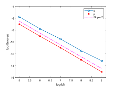
(b) fast fractional CN-BCFD

Figure 1: Errors and convergence orders for Example 4.9 solved by the fractional CN-BCFD scheme and its fast version with fixed $\alpha=1.8$, $\gamma=0.5$

In this simulation, we always take $N=M$ to test the errors of the primal variable $u$ (denoted as ’Error-u’) and its flux $p$ (denoted as ’Error-p’) as well as their convergence orders (Cov.). In Table 1, we list the discrete maximum-norm errors and convergence orders with the chosen parameter $\xi=1/3$, and we also depict the convergence orders of the developed fractional CN-BCFD scheme (2.18) and its fast version (3.17) in Figure 1. We can observe that the fast version fractional CN-BCFD scheme (3.17) generates numerical solutions with the same accuracy as the fractional CN-BCFD scheme (2.18), and the primal variable $u$ and its flux $p$ all have second-order convergence with respect to the discrete maximum-norm for $\alpha=1.8$ and $\gamma=0.5$ (i.e., the fractional operator is symmetric). Therefore, we conclude that, when the true solution has sufficient smoothness, the newly developed schemes can achieve second-order accuracy on nonuniform grids.

Example 4.10.

In this example, we take the spatial interval as $[a,b]=[0,2]$ and the time interval as $[0,T]=[0,1]$. Let $K^{x,L}=t\,(5+x^{\alpha})$ and $K^{x,R}=t\left(5+(2-x)^{\alpha}\right)$ such that the true solution and its flux of model (2.1) are given by

$$u(x,t) =e^{-t}x^{2}(2-x)^{2},$$

$$p(x,t) =\gamma te^{-t}\left[\frac{40x^{3-\alpha}}{\Gamma(4-\alpha)}-\frac{120x^{4-\alpha}}{\Gamma(5-\alpha)}+\frac{120x^{5-\alpha}}{\Gamma(6-\alpha)}+\frac{8x^{3}}{\Gamma(4-\alpha)}-\frac{24x^{4}}{\Gamma(5-\alpha)}+\frac{24x^{5}}{\Gamma(6-\alpha)}\right]$$

$$\qquad+(1-\gamma)te^{-t}\left[-\frac{40(2-x)^{3-\alpha}}{\Gamma(4-\alpha)}+\frac{120(2-x)^{4-\alpha}}{\Gamma(5-\alpha)}-\frac{120(2-x)^{5-\alpha}}{\Gamma(6-\alpha)}\right.$$

$$\left.\qquad\qquad\qquad\qquad-\frac{8(2-x)^{3}}{\Gamma(4-\alpha)}+\frac{24(2-x)^{4}}{\Gamma(5-\alpha)}-\frac{24(2-x)^{5}}{\Gamma(6-\alpha)}\right].$$

First, we choose $M=2^{8}$, $N=2^{12}$ and $\alpha=1.5$, $\gamma=0.5$ to test the errors between the analytical solutions and their numerical approximations under uniform grids (i.e., $\kappa=1$ in (4.2)). The pointwise errors of $u$ at final time $T=1$ are shown in Figure 2 (a) and (c) respectively for the fractional CN-BCFD scheme (2.18) and its fast version (3.17). It reveals that the error mainly comes from the neighbor of boundary points. Thus, when weak singularity occurs in model (2.1), the developed fractional BCFD methods with or without the fast SOE approximation may not work very well as expected and may also lose accuracy. To improve the convergence, one can employ the locally refined grids in the spatial discretization instead of uniform grids to reduce the computational errors. For example, we consider the following graded grids generated as below:

$$x_{i}=\left\{\begin{aligned} &a+\gamma^{1-\kappa}(b-a)\left(\frac{i}{M}\right)^{\kappa},&0\leqslant i\leqslant\lfloor\gamma M\rfloor,\\ &b-(1-\gamma)^{1-\kappa}(b-a)\left(\frac{M-i}{M}\right)^{\kappa},&\lfloor\gamma M\rfloor<i\leqslant M,\end{aligned}\right.$$ (4.2)

where $\lfloor\gamma M\rfloor$ means the largest integer that less than or equal to $\gamma M$, and $\kappa$ is a user-defined graded parameter. It can be seen from Figure 2 (b) and (d) that the errors are significantly reduced when using the graded grids (i.e., $\kappa=1.5$) compared with the uniform case (i.e., $\kappa=1$) .

(a) $\kappa=1$

(b) $\kappa=1.5$

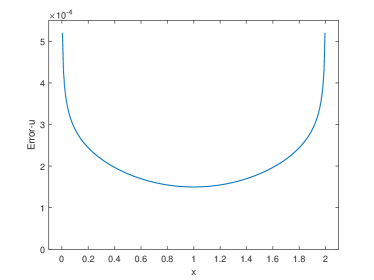
(c) $\kappa=1$

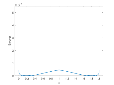
(d) $\kappa=1.5$

Figure 2: Error profiles for Example 4.10 at final time $T=1$ solved by the fractional CN-BCFD scheme (the first row) and the fast fractional CN-BCFD scheme (the second row) with fixed $\alpha=1.5$, $\gamma=0.5$

Table 2: Errors and convergence orders of $u$ for Example 4.10 solved by the fractional CN-BCFD scheme and its fast version with fixed $\alpha=1.5$, $\gamma=0.5$

Method	$M$	$\kappa=1$		$\kappa=1.5$		$\kappa=2$
		Error-u	Cov.	Error-u	Cov.	Error-u	Cov.
	$2^{5}$	5.4058e-03	—	3.0553e-03	—	6.5626e-03	—
fractional	$2^{6}$	2.6623e-03	1.0218	7.5680e-04	2.0134	2.0684e-03	1.6658
CN-BCFD	$2^{7}$	1.2029e-03	1.1462	1.8648e-04	2.0209	6.5705e-04	1.6544
	$2^{8}$	5.2022e-04	1.2093	4.5861e-05	2.0237	2.0973e-04	1.6474
	$2^{9}$	2.1933e-04	1.2460	1.1889e-05	1.9477	6.7128e-05	1.6436
	$2^{5}$	5.4058e-03	—	3.0553e-03	—	6.5626e-03	—
fast fractional	$2^{6}$	2.6623e-03	1.0218	7.5679e-04	2.0134	2.0684e-03	1.6658
CN-BCFD	$2^{7}$	1.2029e-03	1.1462	1.8647e-04	2.0209	6.5700e-04	1.6545
	$2^{8}$	5.2022e-04	1.2093	4.5852e-05	2.0239	2.0963e-04	1.6481
	$2^{9}$	2.1933e-04	1.2460	1.1792e-05	1.9591	6.6807e-05	1.6497

Table 3: Errors and convergence orders of $p$ for Example 4.10 solved by the fractional CN-BCFD scheme and its fast version with fixed $\alpha=1.5$, $\gamma=0.5$

Method	$M$	$\kappa=1$		$\kappa=1.5$		$\kappa=2$
		Error-p	Cov.	Error-p	Cov.	Error-p	Cov.
	$2^{5}$	5.4501e-03	–	2.3359e-03	–	2.7983e-03	–
fractional	$2^{6}$	2.0828e-03	1.3878	6.3144e-04	1.8873	7.1462e-04	1.9693
CN-BCFD	$2^{7}$	7.8032e-04	1.4164	1.6775e-04	1.9123	1.8041e-04	1.9859
	$2^{8}$	2.8837e-04	1.4362	4.4015e-05	1.9303	4.5367e-05	1.9916
	$2^{9}$	1.0562e-04	1.4490	1.1442e-05	1.9436	1.1381e-05	1.9951
	$2^{5}$	5.4501e-03	–	2.3359e-03	–	2.7983e-03	–
fast fractional	$2^{6}$	2.0828e-03	1.3878	6.3144e-04	1.8872	7.1462e-04	1.9693
CN-BCFD	$2^{7}$	7.8032e-04	1.4164	1.6776e-04	1.9123	1.8042e-04	1.9858
	$2^{8}$	2.8836e-04	1.4362	4.4024e-05	1.9300	4.5371e-05	1.9915
	$2^{9}$	1.0561e-04	1.4492	1.1456e-05	1.9422	1.1374e-05	1.9961

Next, we proceed to investigate the influence of the graded parameter $\kappa$ on convergence. We choose $N=2^{12}$ large enough to observe the spatial convergence order for Example 4.10. Numerical results are list in Tables 2–3 with respect to different choices of grid parameters $\kappa$ for fixed $\alpha=1.5$, $\gamma=0.5$. We can observe that the fast version fractional CN-BCFD scheme (3.17) still generates the similar accurate numerical solutions as the fractional CN-BCFD scheme (2.18). Furthermore, it can be seen that for the solution that not smooth enough, the primal variable $u$ and its flux $p$ both have a poor accuracy compared with Example 4.9 on the uniform grids, see Tables 1 and 2–3 with $\kappa=1$. In contrast, these two schemes can achieve second-order accuracy by properly adopting suitable nonuniform spatial grids, such as the grid parameters $\kappa=1.5$. However, it is worth noting that the large grid parameter may also increase the errors. For instance, Table 2 shows that the errors generated via $\kappa=2$ is larger than that of $\kappa=1.5$. Therefore, how to select appropriate grid parameter to achieve optimal error results is still a challenging and interesting work. Finally, we depict the errors of primal variable $u$ and its flux $p$ with different fractional order $\alpha$, weighted parameter $\gamma$ and grid parameter $\kappa$ in Figures 3–4. It indicates that the usage of graded grids (the weighted parameter $\kappa$) for given $\alpha$ and $\gamma$ can significantly improve the accuracy. In addition, the results obtained for the case that the fractional operator is symmetric (i.e., $\gamma=0.5$) are usually better than other cases. In a word, when low regularity or even weak singularity occurs in the solution, it is better to use nonuniform grids to obtain numerical results with much better accuracy, and our developed fast CN-BCFD method is well suited for general nonuniform grids. However, the reasonable choice of nonuniform grids (e.g., (4.2)) usually depends on some a priori regularity information of the solution to (2.1), and as pointed out in Ref. [8] that the solution to the space-fractional diffusion equations even with smooth coefficients and source terms exhibits nonphysical singularities on the spatial boundaries.

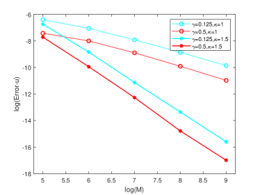
(a) $\alpha=1.8$

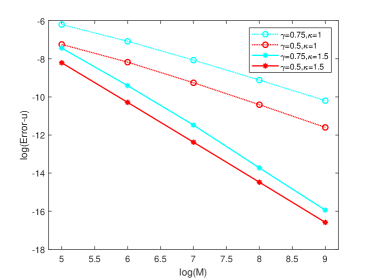
(b) $\alpha=1.6$

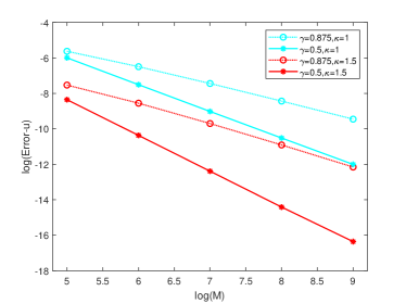
(c) $\alpha=1.5$

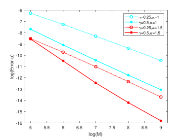
(d) $\alpha=1.3$

Figure 3: Errors of $u$ for Example 4.10 solved by the fast fractional CN-BCFD scheme with different fractional order $\alpha$, weighted parameter $\gamma$ and grid parameter $\kappa$

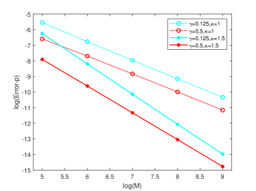
(a) $\alpha=1.8$

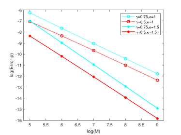
(b) $\alpha=1.6$

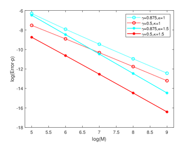
(c) $\alpha=1.5$

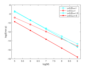
(d) $\alpha=1.3$

Figure 4: Errors of $p$ for Example 4.10 solved by the fast fractional CN-BCFD scheme with different fractional order $\alpha$, weighted parameter $\gamma$ and grid parameter $\kappa$

Example 4.11.

For the third example, we proceed to investigate the performance of the proposed fractional CN-BCFD scheme (2.18) and the fast fractional CN-BCFD scheme (3.17) with a low regularity solution

$$u(x,t)=4e^{t}x^{\frac{\alpha}{2}}(1-x)^{\frac{\alpha}{2}},\quad x\in[0,1],\ t\in[0,1].$$

Here we choose $K^{x,L}=K^{x,R}=t\left(1+x(1-x)\right)$, and the flux $p$ is

$$p(x,t)=4te^{t}\Gamma(\alpha+1)\cos(\alpha\pi/2)\left(1+x(1-x)\right)(x-1/2).$$

(a) $\kappa=1$

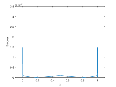
(b) $\kappa=1.5$

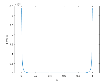
(c) $\kappa=1$

(d) $\kappa=1.5$

Figure 5: Error profiles for Example 4.11 at final time $T$ solved by the fractional CN-BCFD scheme (the first row) and the fast fractional CN-BCFD scheme (the second row) with fixed $\alpha=1.4$, $\gamma=0.5$

To start with, we choose $M=2^{8}$ and $N=2^{12}$ to test the pointwise errors between exact solutions and numerical solutions at final time $T=1$ with fixed $\alpha=1.4$ and $\gamma=0.5$. Similar as Example 4.10, we conclude from Figure 5 that the errors are mainly from the neighbor of boundary points, and the usage of graded grids (i.e. $\kappa=1.5$) clearly improves the accuracy. Then, we present the discrete maximum-norm errors and corresponding convergence orders in Tables 4–5, respectively, for the primal variable $u$ and its flux $p$. It can be seen that the usage of graded grids results in significantly smaller errors than that of uniform grid (i.e. $\kappa=1$) near the boundary. Nevertheless, the convergence orders cannot reach two for the variable $u$ despite the usage of graded grids, while the flux $p$ can achieve second-order accuracy on the graded grids. Meanwhile, the larger grid parameter $\kappa$ will yield a reduction of accuracy. For example, the errors of $\kappa=2$ is obviously bigger than that of $\kappa=1.5$.

Table 4: Errors and convergence orders of $u$ for Example 4.11 solved by the fractional CN-BCFD scheme and and its fast version with fixed $\alpha=1.4$, $\gamma=0.5$

Method	$M$	$\kappa=1$		$\kappa=1.5$		$\kappa=2$
		Error-u	Cov.	Error-u	Cov.	Error-u	Cov.
	$2^{6}$	9.6150e-03	–	1.0497e-02	–	1.7792e-02	–
fractional	$2^{7}$	5.6731e-03	0.7611	3.9111e-03	1.4243	6.7802e-03	1.3918
CN-BCFD	$2^{8}$	3.3787e-03	0.7477	1.4545e-03	1.4271	2.5782e-03	1.3950
	$2^{9}$	2.0309e-03	0.7343	5.4477e-04	1.4168	9.7900e-04	1.3970
	$2^{10}$	1.2299e-03	0.7236	2.0697e-04	1.3962	3.7130e-04	1.3987
	$2^{6}$	9.6152e-03	–	1.0497e-02	–	1.7792e-02	–
fast fractional	$2^{7}$	5.6733e-03	0.7611	3.9113e-03	1.4243	6.7805e-03	1.3917
CN-BCFD	$2^{8}$	3.3789e-03	0.7476	1.4547e-03	1.4269	2.5796e-03	1.3943
	$2^{9}$	2.0315e-03	0.7340	5.4524e-04	1.4157	9.8528e-04	1.3885
	$2^{10}$	1.2360e-03	0.7232	2.0791e-04	1.3909	3.5591e-04	1.4690

Table 5: Errors and convergence orders of $p$ for Example 4.11 solved by the fractional CN-BCFD scheme and its fast version with fixed $\alpha=1.4$, $\gamma=0.5$

Method	$M$	$\kappa=1$		$\kappa=1.5$		$\kappa=2$
		Error-p	Cov.	Error-p	Cov.	Error-p	Cov.
	$2^{6}$	1.4694e-04	–	1.2299e-04	–	3.2002e-04	–
fractional	$2^{7}$	4.3279e-05	1.7635	2.8846e-05	2.0910	8.0726e-05	1.9871
CN-BCFD	$2^{8}$	1.2946e-05	1.7412	6.8784e-06	2.0682	2.0309e-05	1.9909
	$2^{9}$	3.9117e-06	1.7266	1.6597e-06	2.0512	5.0978e-06	1.9942
	$2^{10}$	1.3650e-06	1.5189	4.0339e-07	2.0407	1.2767e-06	1.9974
	$2^{6}$	1.4691e-04	–	1.2288e-04	–	3.2002e-04	–
fast fractional	$2^{7}$	4.3275e-05	1.7633	2.8830e-05	2.0916	8.0724e-05	1.9871
CN-BCFD	$2^{8}$	1.2943e-05	1.7414	6.8699e-06	2.0692	2.0322e-05	1.9900
	$2^{9}$	3.9051e-06	1.7287	1.6487e-06	2.0589	5.1767e-06	1.9729
	$2^{10}$	1.4492e-06	1.4301	3.9197e-07	2.0725	9.8745e-07	2.3903

Example 4.12.

Through this example, we mainly aim to verify the efficiency of the proposed fast fractional CN-BCFD method for the approximation of the SFDE (2.1) with different fractional order $\alpha$ and grid parameter $\kappa$. In this example, the diffusivity coefficients $K^{x,L}=K^{x,R}=x(2-x)$, and the true solution is given by

$$u(x,t)=4tx(2-x),\quad x\in[0,2],\ t\in[0,1].$$

In Tables 6–7, we present the errors and CPU times for the fractional CN-BCFD scheme (2.18) solved by the Gauss elimination solver (denoted as CN-BCFD-GE), the fractional CN-BCFD scheme (2.18) solved by the BiCGSTAB iterative solver (denoted as CN-BCFD-BiCGSTAB) and the fast fractional CN-BCFD scheme (3.17) solved by the fast version BiCGSTAB iterative solver (denoted as CN-BCFD-fBiCGSTAB) via Algorithm 2. Meanwhile, the average number of iterations (Itr.) are also shown for the iterative solver. We can reach the following observations: (i) All these methods generate almost the identical numerical solutions; (ii) The fast version CN-BCFD-fBiCGSTAB algorithm takes significantly less CPU time than the other two algorithms, especially for large-scale modeling. For example, in the case of $\alpha=1.8$, $\kappa=1$, $M=2^{11}$, the CPU time consumed by the CN-BCFD-GE algorithm is more than $46$ hours. In contrast, the fast version CN-BCFD-fBiCGSTAB algorithm only costs no more than 3 minutes; (iii) The use of nonuniform grids does not affect the computational accuracy of the CN-BCFD-fBiCGSTAB algorithm, while compared to the other two algorithms, it is still the most efficient one. In summary, all these results show the superiority of the CN-BCFD-fBiCGSTAB algorithm.

Table 6: Performance of the fractional CN-BCFD schemes solved by different solvers for Example 4.12 with fixed $N=2^{12},\alpha=1.8,\ \kappa=1$

Algorithm	M	Error-u	CPU	Itr.
	$2^{7}$	1.1985e-02	4.63s
	$2^{8}$	6.7979e-03	39s
CN-BCFD-GE	$2^{9}$	3.7886e-03	692s=11m 32s
	$2^{10}$	2.0818e-03	5189s=1h 26m 29s
	$2^{11}$	1.1304e-03	166821s= 46h 20m 21s
	$2^{7}$	1.1985e-02	0.64s	2.00
	$2^{8}$	6.7979e-03	2.86s	2.65
CN-BCFD-BiCGSTAB	$2^{9}$	3.7886e-03	20.15s	5.06
	$2^{10}$	2.0818e-03	171s	9.67
	$2^{11}$	1.1304e-03	4626s=1h 17m 6s	18.97
	$2^{7}$	1.1985e-02	1.10s	2.00
	$2^{8}$	6.7979e-03	2.56s	2.64
CN-BCFD-fBiCGSTAB	$2^{9}$	3.7886e-03	8.71s	5.06
	$2^{10}$	2.0818e-03	31.83s	9.68
	$2^{11}$	1.1304e-03	157s=2m 37s	18.94

Table 7: Performance of the fractional CN-BCFD schemes solved by different solvers for Example 4.12 with fixed $N=2^{12}$, $\alpha=1.6$, $\kappa=1.5$

Algorithm	M	Error-u	CPU	Itr.
	$2^{7}$	2.9450e-03	4.49s
	$2^{8}$	1.1803e-03	40s
CN-BCFD-GE	$2^{9}$	4.7160e-04	693s=11m 33s
	$2^{10}$	1.8695e-04	5180s=1h 26m 20s
	$2^{11}$	7.3360e-05	197474s=54h 51m 14s
	$2^{7}$	2.9450e-03	0.46s	2.00
	$2^{8}$	1.1803e-03	2.21s	2.00
CN-BCFD-BiCGSTAB	$2^{9}$	4.7158e-04	9s	2.00
	$2^{10}$	1.8695e-04	56s	3.51
	$2^{11}$	7.3333e-05	2540s=42m 20s	5.50
	$2^{7}$	2.9450e-03	3.15s	2.00
	$2^{8}$	1.1803e-03	5.98s	2.00
CN-BCFD-fBiCGSTAB	$2^{9}$	4.7158e-04	12s	2.00
	$2^{10}$	1.8695e-04	35s	3.53
	$2^{11}$	7.3329e-05	93s=1m 33s	5.31

4.2 Numerical results for two-dimensional SFDEs

Example 4.13.

In this example, we extend our discussion to the two-dimensional case (1.1). Let $K^{x,L}=K^{x,R}=K^{y,L}=K^{y,R}=1$, and $f(x,y,t)$ is properly chosen such that the true solution of model (1.1) is given by

$$u(x,y,t)=e^{t}x^{2}(2-x)^{2}y^{2}(2-y)^{2},\quad x\in[0,2]^{2},\ t\in[0,1].$$

Table 8: Performance of the fractional CN-BCFD schemes solved by different solvers for the two-dimension SFDE with different $\alpha$, $\beta$ and fixed $N=2^{10},\kappa=1$

$(\alpha,\beta)$	$M_{x}=M_{y}$	CN-BCFD-GE		CN-BCFD-fBiCGSTAB
		Error-u	CPU	Error-u	CPU	Itr.
	$2^{5}$	2.7164e-02	2055s = 34m 15s	2.2680e-02	72s=1m 12s	3.00
$(1.5,1.5)$	$2^{6}$	1.1978e-02	574261s$\approx$7d	1.1884e-02	270s=4m 30s	4.00
	$2^{7}$	—	—	6.0684e-03	755s=12m 35s	5.00
	$2^{8}$	—	—	3.0603e-03	2819s=46m 59s	8.01
	$2^{5}$	2.1504e-02	1811s=30m 11s	2.0971e-02	80s=1m 20s	3.00
$(1.4,1.7)$	$2^{6}$	—	—	1.1402e-02	258s=4m 18s	5.00
	$2^{7}$	—	—	6.0605e-03	1092s=18m 12s	8.00
	$2^{8}$	—	—	3.1988e-03	4969s=1h 22m 49s	14.00
	$2^{5}$	1.6065e-02	1285s=21m 25s	1.6006e-02	100s=1m 40s	4.00
$(1.6,1.9)$	$2^{6}$	—	—	8.4224e-03	361s=6m 1s	7.00
	$2^{7}$	—	—	4.3937e-03	2773s=46m 13s	14.00
	$2^{8}$	—	—	2.2723e-03	9434s=2h 37m 14s	27.14

In this simulation, we fix $N=2^{10}$ and test different combinations of $(\alpha,\beta)$ and $\kappa$ for the comparisons of the developed BCFD schemes for the two-dimensional model (1.1). In Tables 8–9, we present the errors and CPU times for the CN-BCFD-GE algorithm and the fast version CN-BCFD-fBiCGSTAB algorithm. Meanwhile, the average numbers of iterations per time level for the latter one are also list. As the one-dimensional case, it is seen that both algorithms generate the same accurate numerical solutions whether on uniform or nonuniform grids. Besides, it also shows that the usage of graded grids evidently improves the computational accuracy, see comparisons of the results in Tables 8–9. In addition, the fast version CN-BCFD-fBiCGSTAB algorithm shows an efficient and effective capability for solving the two-dimensional model. For example, with $(\alpha,\beta)=(1.5,1.5)$, $\kappa=1$, and $M_{x}=M_{y}=2^{6}$, the CN-BCFD-GE algorithm spends around 7 days to reach the error of magnitude $10^{-2}$ , while the CN-BCFD-fBiCGSTAB algorithm consumes only no more than 5 minutes for the nearly same error. However, for larger-scale modeling, for example, $(\alpha,\beta)=(1.5,1.5)$, $M_{x}=M_{y}=2^{8}$ and $\kappa=1.5$, the CN-BCFD-GE algorithm can hardly run on the computer, but the CN-BCFD-fBiCGSTAB algorithm can still achieve the error of magnitude $10^{-4}$ in only three and a half hours. It is believed that the comparisons shall be more obvious for even larger $M_{x}$ and $M_{y}$. Finally, we would like to point out that with the increasing number of grids, the average number of iterations becomes larger and larger especially on the nonuniform grids, see Table 9. This in turn increases the overall computational cost. Therefore, it is of great importance to develop an efficient preconditioning technique for the resulting linear algebraic system [15, 13, 5, 22, 12, 42, 10, 26, 37]. To sum up, numerical results for the two-dimensional model further demonstrate the strong superiority of the CN-BCFD-fBiCGSTAB algorithm in large-scale modeling and simulation.

Table 9: Performance of the fractional CN-BCFD schemes solved by different solvers for the two-dimension SFDE with different $\alpha$, $\beta$ and fixed $N=2^{10},\kappa=1.5$

$(\alpha,\beta)$	$M_{x}=M_{y}$	CN-BCFD-GE		CN-BCFD-fBiCGSTAB
		Error-u	CPU	Error-u	CPU	Itr.
	$2^{5}$	1.8287e-02	2809s=46m 49s	1.8302e-02	123s=2m 3s	4.66
$(1.5,1.5)$	$2^{6}$	—	—	4.9508e-03	548s=9m 8s	7.06
	$2^{7}$	—	—	2.1587e-03	2263s=37m 43s	13.90
	$2^{8}$	—	—	9.9896e-04	12818s=3h 33m 38s	31.20
	$2^{5}$	1.7733e-02	1286s=21m26s	1.7752e-02	140s=2m 20s	5.00
$(1.4,1.7)$	$2^{6}$	—	—	4.7589e-03	753s=12m 33s	10.00
	$2^{7}$	—	—	1.6591e-03	3856s=1h 4m 16s	23.41
	$2^{8}$	—	—	7.9748e-04	26447s=7h 20m 47s	58.49
	$2^{5}$	1.7347e-02	1284s=21m 24s	1.7359e-02	189s=3m 9s	7.01
$(1.6,1.9)$	$2^{6}$	—	—	4.4954e-03	1152s=19m 12s	17.67
	$2^{7}$	—	—	1.1314e-03	8287s=2h 18m 7s	47.62
	$2^{8}$	—	—	2.7873e-04	59480s=16h 31m 20s	139.67

5 Conclusions

This paper seems to be the first attempt to discuss fractional BCFD method and its efficient implementation for both one and two-dimensional SFDEs with fractional Neumann boundary condition on general nonuniform grids. Totally different from the case of uniform spatial partitions, where Toeplitz-like matrix structure can be discovered for the widely used numerical methods such as finite difference and finite volume methods, and that would lead to significantly reduced memory requirement and computational complexity. The developed fractional BCFD method is well suitable for the nonuniform grids, and based upon the SOE approximation technique, a fast version fractional BCFD algorithm is further constructed, in which fast matrix-vector multiplications of the resulting coefficient matrices with any vector in only $\mathcal{O}(MN_{exp})$ operations are developed. Numerical experiments show that the usage of locally refined grids greatly improves the accuracy of the developed method, and most importantly, the fast version CN-BCFD-fBiCGSTAB algorithm has greatly reduced the CPU times without any accuracy being lost. The method shows strong potential in large-scale modeling and simulation of high-dimensional SFDEs. It is still a challenging work to study the preconditioning strategy to further reduce the computational complexity in the near future.

Declarations

• Funding  This work is supported in part by funds from the National Natural Science Foundation of China Nos. 11971482 and 12131014, the Fundamental Research Funds for the Central Universities No. 202264006, the OUC Scientific Research Program for Young Talented Professionals.

• Data availability  Enquiries about data availability should be directed to the authors.

• Conflict of interest  The authors declare that they have no competing interests.

• Author contributions  Meijie Kong: Formal analysis, Investigation, Methodology, Visualization, Writing–original draft. Hongfei Fu: Conceptualization, Funding acquisition, Methodology, Supervision, Writing–review editing.

References

- [1] B. Baeumer, M. Kovcs, M. M. Meerschaert, R. L. Schilling, and P. Straka. Reflected spectrally negative stable processes and their governing equations. Trans. Am. Math. Soc., 368(1):227–248, 2015.
- [2] R. Barrett, M. Berry, T. F. Chan, J. Demmel, J. M. Donato, J. Dongarra, V. Eijkhout, R. Pozo, C. Romine, and H. V. der Vorst. Templates for the solution of linear systems: building blocks for iterative methods. SIAM, 1994.
- [3] D. Benson, S. W. Wheatcraft, and M. M. Meerschaert. The fractional-order governing equation of lévy motion. Water Resour Res., 36(6):1413–1423, 2000.
- [4] W. Chen, Y. Liang, S. Hu, and H. Sun. Fractional derivative anomalous diffusion equation modeling prime number distribution. Fract. Calc. Appl. Anal., 18(3):789–798, 2015.
- [5] P. Dai, J. Jia, H. Wang, Q. Wu, and X. Zheng. An efficient positive-definite block-preconditioned finite volume solver for two-sided fractional diffusion equations on composite mesh. Numer. Linear Algebra Appl., 28(5):e2372, 2021.
- [6] K. Diethelm, N. J. Ford, and A. D. Freed. A predictor-corrector approach for the numerical solution of fractional differential equations. Nonlinear Dynamics, 29(1-4):3–22, 2002.
- [7] K. Diethelm, N. J. Ford, and A. D. Freed. Detailed error analysis for a fractional Adams method. Numerical algorithms, 36(1):31–52, 2004.
- [8] V. J. Ervin, N. Heuer, and J. P. Roop. Regularity of the solution to 1-D fractional order diffusion equations. Math. Comput., 87(313):2273–2294, 2018.
- [9] V. J. Ervin and J. P. Roop. Variational formulation for the stationary fractional advection dispersion equation. Numer. Methods Partial Differential Equ., 22(3):558–576, 2006.
- [10] Z. Fang, H. Sun, and H. Wei. An approximate inverse preconditioner for spatial fractional diffusion equations with piecewise continuous coefficients. Int. J. Comput. Math., 97(3):523–545, 2020.
- [11] Z. Fang, J. Zhang, and H. Sun. A fast finite volume method for spatial fractional diffusion equations on nonuniform meshes. Comput. Math. Appl., 108:175–184, 2022.
- [12] H. Fu, H. Liu, and H. Wang. A finite volume method for two-dimensional Riemann-Liouville space-fractional diffusion equation and its efficient implementation. J. Comput. Phys., 388:316–334, 2019.
- [13] H. Fu and H. Wang. A preconsitioned fast finite difference method for space-time fractional partial differential equations. Fract. Calc. Appl. Anal., 20(1):88–116, 2017.
- [14] Z. Hao, M. Park, G. Lin, and Z. Cai. Finite element method for two-sided fractional differential equations with variable coefficients: Galerkin approach. J. Sci. Comput., 79(2):700–717, 2019.
- [15] J. Jia and H. Wang. A preconditioned fast finite volume scheme for a fractional differential equation discretized on a locally refined composite mesh. J. Comput. Phys., 299:842–862, 2015.
- [16] J. Jia and H. Wang. A fast finite volume method for conservative space-time fractional diffusion equations discretized on space-time locally refined meshes. Comput. Math. Appl., 78(5):1345–1356, 2019.
- [17] S. Jiang, J. Zhang, Q. Zhang, and Z. Zhang. Fast evaluation of the Caputo fractional derivative and its applications to fractional diffusion equations. Commun. Comput. Phys., 21(3):650–678, 2017.
- [18] B. Jin, R. Lazarov, J. Pasciak, and W. Rundell. Variational formulation of problems involving fractional order differential operators. Math. Comput., 84(296):2665–2700, 2015.
- [19] B. Jin, R. Lazarov, and Z. Zhou. An analysis of the L1 scheme for the subdiffusion equation with nonsmooth data. IMA J. Numer. Anal., 36(1):197–221, 2015.
- [20] H. Liu, X. Zheng, H. Fu, and H. Wang. Analysis and efficient implementation of alternating direction implicit finite volume method for Riesz space-fractional diffusion equations in two space dimensions. Numer. Methods Partial Differ. Equ., 37(1):818–835, 2021.
- [21] H. Liu, X. Zheng, H. Wang, and H. Fu. Error estimate of finite element approximation for two-sided space-fractional evolution equation with variable coefficient. J. Sci. Comput., 90(1):1–19, 2022.
- [22] J. Liu, H. Fu, H. Wang, and X. Chai. A preconditioned fast quadratic spline collocation method for two-sided space-fractional partial differential equations. J. Comput. Appl. Math., 360:138–156, 2019.
- [23] Z. Liu and X. Li. A parallel CGS block-centered finite difference method for a nonlinear time-fractional parabolic equation. Comput. Methods Appl. Mech. Engrg., 308:330–348, 2016.
- [24] Z. Mao and J. Shen. Efficient spectral-Galerkin methods for fractional partial differential equations with variable coefficients. J. Comput. Phys., 307:243–261, 2016.
- [25] R. Metzler and J. Klafter. The random walk’s guide to anomalous diffusion: a fractional dynamics approach. Phys. Rep., 339(1):1–77, 2000.
- [26] J. Pan, R. Ke, M. K. Ng, and H. Sun. Preconditioning techniques for diagonal-times-Toeplitz matrices in fractional diffusion equations. SIAM J. Sci. Comput., 36(6):A2698–A2719, 2014.
- [27] K. Pan, H. Sun, Y. Xu, and Y. Xu. An efficient multigrid solver for two-dimensional spatial fractional diffusion equations with variable coefficients. Appl. Math. Comput., 402:126091, 2021.
- [28] I. Podlubny. Fractional Differential Equations. Academic Press, New York, 1999.
- [29] P. A. Raviart and J. M. Thomas. A mixed finite element method for 2nd order elliptic problems. In Lecture Notes in Mathematics, pages 292–315. Springer, New York, 1977.
- [30] H. Rui and H. Pan. A block-centered finite difference method for the Darcy-Forchheimer model. SIAM J. Numer. Anal., 50(5):2612–2631, 2012.
- [31] A. Simmons, Q. Yang, and T. Moroney. A finite volume method for two-sided fractional diffusion equations on non-uniform meshes. J. Comput. Phys., 335:747–759, 2017.
- [32] M. Stynes, E. O’Riordan, and J. L. Gracia. Error analysis of a finite difference method on graded meshes for a time-fractional diffusion equation. SIAM J. Numer. Anal., 55(2):1057–1079, 2017.
- [33] H. Sun, A. Chang, Y. Zhang, and W. Chen. A review on variable-order fractional differential equations: mathematical foundations, physical models, and its applications. Fract. Calc. Appl. Anal., 22(1):27–59, 2018.
- [34] H. Sun, Y. Zhang, W. Chen, and D. M. Reeves. Use of a variable-index fractional-derivative model to capture transient dispersion in heterogeneous media. J. Contaminant Hydrology, 157:47–58, 2014.
- [35] W. Tian, H. Zhou, and W. Deng. A class of second order difference approximations for solving space fractional diffusion equations. Math. Comput., 84(294):1703–1727, 2015.
- [36] H. Wang and T. S. Basu. A fast finite difference method for two-dimensional space-fractional diffusion equations. SIAM J. Sci. Cumput., 34(5):A2444–A2458, 2012.
- [37] H. Wang and N. Du. A superfast-preconditioned iterative method for steady-state space-fractional diffusion equations. J. Comput. Phys., 240:49–57, 2013.
- [38] H. Wang and K. Wang. An alternating-direction finite difference method for two-dimensional fractional diffusion equations. J. Comput. Phys., 230(21):7830–7839, 2011.
- [39] H. Wang, K. Wang, and T. Sircar. A direct finite difference method for fractional diffusion equations. J. Comput. Phys., 229(21):8095–8104, 2010.
- [40] M. Wang, H. Wang, and A. Cheng. A fast finite difference method for three-dimensional time-dependent space-fractional diffusion equations with fractional derivative boundary conditions. J. Sci. Comput., 74(2):1009–1033, 2018.
- [41] J. Xu, S. Xie, and H. Fu. A two-grid block-centered finite difference method for the nonlinear regularized long wave equation. Appl. Numer. Math., 171:128–148, 2022.
- [42] Y. Xu, S. Lei, and H. Sun. An efficient multigrid method with preconditioned smoother for two-dimensional anisotropic space-fractional diffusion equations. Comput. Math. Appl., 124:218–226, 2022.
- [43] Y. Yan, M. Khan, and N. J. Ford. An analysis of the modified L1 scheme for time-fractional partial differential equations with nonsmooth data. SIAM J. Numer.Anal., 56(1):210–227, 20178.
- [44] Y. Yan, Z. Sun, and J. Zhang. Fast evaluation of the Caputo fractional derivative and its applications to fractional diffusion equations: a second-order scheme. Commun. Comput. Phys., 22(4):1028–1048, 2017.
- [45] F. Zeng, F. Liu, C. Li, K. Burrage, I. Turner, and V. Anh. A Crank-Nicolson ADI spectral method for a two-dimensional Riesz space fractional nonlinear reaction-diffusion equation. SIAM J. Numer. Anal., 52(6):2599–2622, 2014.
- [46] F. Zeng, I. Turner, and K. Burrage. A stable fast time-stepping method for fractional integral and derivative operators. J. Sci. Comput., 77(1):283–307, 2018.
- [47] C. Zhu, B. Zhang, H. Fu, and J. Liu. Efficient second-order ADI difference schemes for three-dimensional Riesz space-fractional diffusion equations. Comput. Math. Appl., 98:24–39, 2021.