Minimal Pole Representation and Controlled Analytic Continuation of Matsubara Response Functions

Abstract

Analytic continuation is a central step in the simulation of finite-temperature field theories in which numerically obtained Matsubara data is continued to the real frequency axis for physical interpretation. Numerical analytic continuation is considered to be an ill-posed problem where uncertainties on the Matsubara axis are amplified exponentially. Here, we present a systematic and controlled procedure that approximates any Matsubara function by a minimal pole representation to within a predefined precision. We then show systematic convergence to the exact spectral function on the real axis as a function of our control parameter for a range of physically relevant setups. Our methodology is robust to noise and paves the way towards reliable analytic continuation in many-body theory and, by providing access to the analytic structure of the functions, direct theoretical interpretation of physical properties.

Quantum field theory simulations at finite temperature are typically performed on the Matsubara axis [1]. In a post-processing step, real-frequency information is obtained via analytic continuation for physical interpretation. Simulations that require continuation range from perturbative calculations [2, 3, 4] to lattice [5] and continuous-time [6] quantum Monte Carlo and lattice QCD [7, 8, 9] simulations, as well as algorithms for the simulation of bosonic systems [10] including He [11, 12], supersolids [13], and warm dense matter [14].

Due to the ill-conditioned nature of the analytic continuation step [15], a variety of numerical continuation methods have been developed. Among these are Padé [16] continued fraction fits of Matsubara data [17, 18, 19, 20, 21, 22], an interpolation with Nevanlinna functions [23, 24], the Maximum Entropy (MaxEnt) method [25, 26, 15, 27, 28, 29, 30, 31, 32, 33, 34], sparse modeling [35, 36], stochastic analytic continuation (SAC) and variants [37, 38, 39, 40, 41, 42, 36, 43], genetic algorithms and machine learning [12, 44, 45], causal projections [46] and Prony fits [47, 48]. In all of these methods, it is difficult in practice to systematically converge the spectral function, even given high-precision Matsubara data.

In this Letter, we revisit the continuation problem from the perspective of a compact low-rank representation of response functions in terms of a pole expansion that approximates Matsubara data within a predetermined precision $\varepsilon$. Remarkably, as we show below, the spectral function systematically converges to the exact answer as the precision of the Matsubara fit is increased. Even ‘difficult’ spectral functions containing both sharp and smooth features at low and at high energies are well approximated.

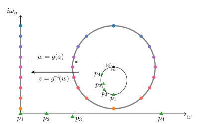
Figure 1: Holomorphic functions $g(z)$ and $g^{-1}(w)$ mapping the complex plane to the unit disk and an interval on the imaginary axis to the unit circle. Also shown are points on and near the real axis as triangles, along with their image under $g$.

The method is generally applicable to all response functions, including diagonal and off-diagonal fermionic and bosonic response functions of continuous and discrete systems. Examining the application of the methodology to data polluted with stochastic noise we find, similarly, that a fit to within the known precision of the input data results in physically reasonable spectral functions that are systematically improved as the uncertainty on the Matsubara axis is reduced.

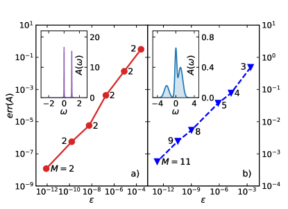
Figure 2: Integrated real axis error $err(A)=\int_{\mathbb{R}}d\omega|A-A_{\text{cont}}|$ for the discrete (left) and continuous (right) case as a function of control parameter $\varepsilon$. Also indicated is the number of poles $M$. Inset: spectrum $A(\omega)$. Other parameters are $\beta=200$, $n_{0}=30\text{ (left)}\text{ and }0\text{ (right)}$, $\Delta n=1$ and $N_{\omega}=2001$.

Theory and Method. We construct an approximation of Matsubara data of the form

$$G(z)=\sum_{l=1}^{M}\frac{A_{l}}{z-\xi_{l}},$$ (1)

where the $\xi_{l}\in\mathbb{C}$ denote $M$ pole locations and $A_{l}\in\mathbb{C}$ the corresponding complex weights, in four steps. First, we approximate Matsubara data on a finite interval of the imaginary axis using Prony’s approximation method [49, 50]. Second, we map this interval onto the unit circle using a holomorphic mapping. We then evaluate the moments of the interpolated function numerically and use Prony’s approximation for a second time to extract a compact representation in terms of pole weights and locations. Finally, we map the poles back onto the original domain and evaluate the spectral function.

Our input data consists of an odd number $N_{\omega}=2N+1$ of Matsubara points $G(i\omega_{n})$ that are uniformly spaced, starting from a minimal non-negative frequency $\omega_{n_{0}}$ with spacing $\Delta n$, i.e., $\{i\omega_{n_{0}},i\omega_{n_{0}+\Delta n},\cdots,i\omega_{n_{0}+(N_{\omega}-1)\Delta n}\}$.

Prony’s interpolation method [49] interpolates $G_{k}$ as $G_{k}=\sum_{i=0}^{N}w_{i}\gamma_{i}^{k}$, where $G_{k}=G(i\omega_{n_{0}+k\Delta n})$, $0\leq k\leq 2N$, $w_{i}$ denote complex weights and $\gamma_{i}$ corresponding nodes.

Prony’s interpolation method is unstable [51]. We therefore employ a Prony approximation [50], rather than an interpolation, of $G$ between $i\omega_{n_{0}}$ and $i\omega_{n_{0}+(N_{\omega}-1)\Delta n}$. For physical Matsubara functions, which decay in magnitude to zero for $i\omega_{n}\rightarrow i\infty$, only $K\propto\log(1/\varepsilon)$ nodes of the Prony interpolation have weight $|w_{i}|>\varepsilon$ [50]. More importantly, $K$ significant nodes can be predetermined [50] such that the solution of the overdetermined $(2N+1)\times K$ problem is stable and yields an accurate solution of the Prony approximation problem

$$\left|G_{k}-\sum_{i=0}^{K-1}w_{i}\gamma_{i}^{k}\right|\leq\varepsilon\text{ for all }0\leq k\leq 2N$$ (2)

for a predefined tolerance $\varepsilon>0$ via singular value decomposition. By varying $k$ continuously over the interval $[0,2N]$, we obtain an approximation of Matsubara data on the continuous interval $[i\omega_{n_{0}},i\omega_{n_{0}+(N_{\omega}-1)\Delta n}]$.

We then apply a holomorphic transform $g(z)$, which is a combination of linear transform and an inverse Joukowsky transform [52] and is illustrated in Fig. 1, to map the complex plane to the closed unit disk.

$$\left\{\begin{array}[]{lll}w\!\!&=g(z)&=z_{\rm s}-\sqrt{z_{\rm s}^{2}+1}\text{ with }z_{\rm s}=\frac{z-i\omega_{\rm m}}{\Delta\omega_{\rm h}}\\ z\!\!&=g^{-1}(w)\!\!&=\frac{\Delta\omega_{\rm h}}{2}(w-\frac{1}{w})+i\omega_{\rm m}\end{array}\right.\;,$$ (5)

where $\omega_{\rm m}=(\omega_{n_{0}}+\omega_{n_{0}+(N_{\omega}-1)\Delta n})/2$ is the frequency in the middle of the approximated interval, $\Delta\omega_{\rm h}=(\omega_{n_{0}+(N_{\omega}-1)\Delta n}-\omega_{n_{0}})/2$ is half of the segment length, and the branch of the square root in the first equation is chosen such that $|w|\leq 1$. The interpolated Matsubara interval forms the unit circle, with $g(i\omega_{n_{0}})=-i$, $g(i\omega_{n_{0}+(N_{\omega}-1)\Delta n})=+i$, and any other point splits into two copies with identical $y$ values. The real axis is mapped onto a closed contour contained in the unit disk with $\infty$ mapped to the origin.

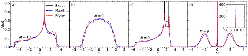
Figure 3: Continuation of continuous spectral functions. From left to right: tight binding density of states of 2d square lattice with nearest- and next-nearest neighbor hopping. Semicircular density of states. Tight-binding density of states of the anisotropic triangular lattice. ‘Kondo’-like spectral function. Shown are the exact input $A(\omega)$ in black, a continuation with Maximum Entropy (blue), and a Prony fit (this method) in red. Maximum Entropy parameters fine-tuned to yield best spectra possible.

Since the transformed response function $\tilde{G}(w)$ corresponds to Eq. 1 as $\tilde{G}(w)=G(z)$ and takes the form

$$\tilde{G}(w)=\sum_{l}\frac{\tilde{A}_{l}}{w-\tilde{\xi}_{l}}+\text{ analytic part}\;,$$ (6)

the integrals over the unit circle

$$h_{k} =\frac{1}{2\pi i}\int_{\partial\bar{D}}\tilde{G}(w)w^{k}dw=\sum_{l}\tilde{A}_{l}\tilde{\xi}_{l}^{k}\;,k\geq 0$$ (7)

yield its moments and, via the residue theorem, pole information [48, 47]. Additional simplification yields

$$h_{k}\!=\!\left\{\begin{array}[]{lll}\!\!\!\!\!&\frac{i}{\pi}\int_{-\frac{\pi}{2}}^{\frac{\pi}{2}}G(i(\omega_{\rm m}+\Delta\omega_{\rm h}\sin\theta))\sin(k+1)\theta d\theta\\ \!\!\!\!\!&\frac{1}{\pi}\int_{-\frac{\pi}{2}}^{\frac{\pi}{2}}G(i(\omega_{\rm m}+\Delta\omega_{\rm h}\sin\theta))\cos(k+1)\theta d\theta\end{array}\right.\;,$$ (10)

for $k$ even and odd, respectively. Using the continuous representation of $G$ obtained in the last step and numerical quadrature, these moments are obtained to high precision. Note that since all $\tilde{\xi}_{l}$ lie within the unit circle, the moments $h_{k}$ decay quickly as a function of $k$ and can be truncated for $h_{k}\ll\varepsilon$.

Eq. 7 forms a second Prony problem. With Eq. 2, $M$ significant $\tilde{A_{l}}$ and $\tilde{\xi}_{l}$ are extracted and the resulting poles and weights are recovered as

$$\xi_{l} =g^{-1}(\tilde{\xi}_{l})=\frac{\Delta\omega_{\rm h}}{2}(\tilde{\xi}_{l}-\frac{1}{\tilde{\xi}_{l}})+i\omega_{\rm m}\;,$$ (11)

$$A_{l} ={\rm Res}[G(z),\xi_{l}]=\frac{\Delta\omega_{\rm h}}{2}(1+\frac{1}{\tilde{\xi}_{l}^{2}})\tilde{A_{l}}\;.$$ (12)

Eqs. 11 and 12 yield a minimal pole approximation of the form of Eq. 1 that is accurate to within $\varepsilon$ and reveals the analytic structure of the function. To evaluate the corresponding spectral function $A(\omega)=-\frac{1}{\pi}\text{Im}G(\omega+i0^{+}),$ we evaluate Eq. 1 for $\omega$ along $\mathbb{R}+i0^{+}$. By lowering $\varepsilon$, the precision can be systematically increased, at the cost of adding additional poles. For the cases examined, this pole representation is much more compact than comparable schemes [53, 54, 55, 56, 57, 58, 59] which typically do not yield a systematically improvable representation of the spectral function and may violate the analytic properties of the response function.

Prony’s method has previously been used to study the analytic continuation problem [48, 47]. The major differences to this work are that Ref. [48] employs a different approximation procedure, either a causal projection onto a finite real-axis grid or a spline interpolation, and different grids and maps, as well as a different solution method of the Prony problem. These steps preclude generality and systematic error control in Ref. [48].

The supplement to this paper contains a pedagogical implementation of this procedure that, given a set of Matsubara points and a tolerance $\varepsilon$, produces a compact representation of the response function and its corresponding spectral function. An open source implementation will also be available as part of the Green software package [60].

Results. We start our discussion with an examination of the convergence of the spectrum as a function of the error control parameter $\varepsilon.$ For a discrete (Fig. 2a) and continuous (Fig. 2b) case we define a spectral function $A(\omega)$ on the real axis, transform it to the Matsubara axis, and continue it back to the real axis within precision $\varepsilon$ as $A_{\text{cont}}$. We then show $err(A)=\int d\omega|A-A_{\text{cont}}|$ as a function of $\varepsilon$. In striking difference to the ‘ill-conditioned’ nature of a direct analytic continuation, we observe that $A_{\text{cont}}$ rapidly converges to $A$ as $\varepsilon$ is decreased. The approximation is indeed compact: in the discrete case, only two poles are needed irrespective of the precision. In the continuum case, increasing the precision of the difference of the integral to $10^{-3}$ requires an increase of the number of poles from $M=3$ to $M=11.$ The supplement contains the precise analytical form of the functions examined along a list of the poles.

In Fig. 3, we analyze the performance of the method for four continuous noiseless scenarios: A continuous spectral function with sharp band edges and a van Hove singularity, as it is encountered in a 2d tight binding calculation of the square lattice with nearest- and next-nearest-neighbor hopping (left panel); a ‘semicircular’ density of states with square-root singularities as encountered in the non-interacting infinite coordination number Bethe lattice with nearest neighbor hopping (middle panel); a tight-binding band structure of an anisotropic triangular lattice [61], and a simulated ‘Kondo’ setup with a sharp peak and two side bands (right panel).

We proceed as in Fig. 2 by back-continuing the known function $A(\omega)$ to the Matsubara axis, interpolating it with $\varepsilon$ chosen close to machine precision (resulting in $M=10$, $9$, $9$, and $9$), and plotting both $A(\omega)$ and $A_{\text{cont}}(\omega)$ as a function of frequency $\omega$ together with a maximum entropy [15, 30] result.

All four functions are difficult to analytically continue with standard methods, since they contain both broad and sharp features. The standard methodology of finding the ‘smoothest’ function consistent with input data within some error is not appropriate and introduces artificial ‘ringing’. While precise knowledge of the location of the band edges and singularities could be used in a Nevanlinna function interpolation [24] followed by a Hardy function optimization [24] to pick the ‘correct’ function out of a Hardy function space, this knowledge is often not available.

The low-rank representation of the Green’s function produced by the Prony method provides an unbiased alternative selection criterion that, in this case, is substantially more precise than a smoothness criterion.

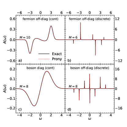
Figure 4: Analytic continuation of non-positive spectral functions. Black: Exact input. Red: Continuation. Panel (a/b): off-diagonal continuous (a) and discrete (b) fermion case. (c) diagonal boson case. (d) discrete off-diagonal boson case.

While a fermion Green’s function of an operator and its corresponding adjoint corresponds to a positive spectral function [62] whose poles lie in the lower half of the complex plane [24], response functions of interest also include bosonic, anomalous, and off-diagonal cases which have different analytical properties. Importantly, they may not correspond to a probability distribution, ruling out the straightforward application of Maximum Entropy and related methods. While the issue can be circumvented by continuing related quantities [63, 64, 65, 66, 67], the procedure often amplifies errors [15].

The method presented here does not explicitly enforce an analytic structure. It can therefore be applied directly to bosonic, off-diagonal, and anomalous Green’s functions as well as to self-energies. As an example we show the off-diagonal part of a continuous fermion spectral function in Fig. 4a; a discrete off-diagonal fermion system in Fig. 4b; a continuous diagonal boson system in Fig. 4c; and a discrete off-diagonal boson system in Fig. 4d. Note that the method for continuous and discrete systems is identical; it is the low-rank representation that places a minimum number of poles very close to the real axis to distinguish sharp (discrete) features from smooth (continuous) ones.

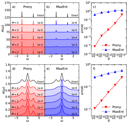
Figure 5: Spectral functions for different levels of Gaussian noise $\delta$ on the imaginary axis. Upper panel: discrete case. Lower panel: continuous case. Also indicated is the number of poles $M$.

Analytic continuation is commonly used on noisy Monte Carlo data, where a response function is known only within a given precision. The precision achievable depends very much on the Monte Carlo algorithm and the estimator used but is rarely better than $10^{-5}$, and errors are often (but not always [68]) Gaussian distributed. In that case, we substitute $\varepsilon$ as a proxy for the Monte Carlo error bar.

For a discrete and a continuous scenario, the left panels of Fig. 5 shows the convergence of the spectral function in our method and in Maximum Entropy [15] for simulated Gaussian errors with varying magnitude. The right panel shows the integrated error $err(A).$ It is evident that already very loose error tolerance reproduces the main features of the spectrum. As the simulated Monte Carlo errors are decreased, our method rapidly converges to the exact result whereas the spectrum is not recovered in Maximum Entropy.

In conclusion, we have shown a method to systematically construct low-rank pole approximations to Matsubara response functions of quantum systems and used it to analytically continue spectral functions. We have demonstrated the control of the method in the sense that the error in the real-frequency response functions can be systematically reduced by improving the corresponding Matsubara fit.

We have also demonstrated the wide applicability of the method, including its suitability for diagonal, off-diagonal, fermionic, bosonic, continuous, and discrete response functions and we have examined the convergence in the presence of noise. We note that the same approximation scheme can also be used to model real-frequency response functions a short distance above the real axis, which may be useful in cases where a Matsubara representation is to be avoided entirely.

Apart from analytic continuation, the compact representations introduced here offer a path towards faster numerical and analytical manipulation of response functions, and they offer physical insight by revealing the locations of poles and zeros in the complex plane.

I Details of numerical simulations

The input of our simulations is an odd number of Matsubara points $G(i\omega_{n})$ sampled on a uniform grid

$$\{i\omega_{n_{0}},i\omega_{n_{0}+\Delta n},\cdots,i\omega_{n_{0}+(N_{\omega}-1)\Delta n}\},$$ (13)

where $\omega_{n}=\frac{(2n+1)\pi}{\beta}$ for fermions and $\frac{2n\pi}{\beta}$ for bosons, $n_{0}\geq 0$ is an integer controlling the number of the first few points we decide to discard (if any), $\Delta n\geq 1$ is an integer controlling the distance of successive sampling points, $N_{\omega}$ is the total number of sampling points and should be an odd number. We find that it is sometimes advantageous to choose $n_{0}$ different from $0$ (for fermions) or $1$ (for bosons). In this case, the final interpolant has to be validated at the discarded points to ensure that they are consistent with the interpolant to within $\varepsilon$.

To achieve best performance, we choose the following heuristic criteria: $n_{0}$ should be chosen as the smallest value so that $\min|i\omega_{n_{0}}-\xi_{l}|$ and $\max|i\omega_{n_{0}}-\xi_{l}|$ are of the same order and function values between first two sampling points, i.e., $G(i\omega_{n_{0}})$ and $G(i\omega_{n_{0}+\Delta n})$, do not change dramatically; $N_{\omega}$ should be chosen to the value making $\{\tilde{\xi_{l}}\}$ separated as far as possible; it is sufficient to set $\Delta n=\max\{1,\frac{\beta}{200}\}$ for the 64-bit machine precision. Spectra should be robust to whatever choice of $n_{0}$ and $N_{\omega}$ is taken. For concreteness, in our simulations we choose $\beta=200$, $N_{\omega}=2001$ and $\Delta n=1$ for all cases; other choices show similar results.

For this paper, unless specified, the Matsubara data is always obtained from a known spectral function $A(\omega)$ via

$$G(i\omega_{n})=\int_{-\infty}^{+\infty}d\omega\frac{A(\omega)}{i\omega_{n}-\omega}\;.$$ (14)

After obtaining pole information by our method, the recovered spectral function is obtained from

$$A_{\rm cont}(\omega)=-\frac{1}{\pi}\imaginary\lim_{\eta\rightarrow 0^{+}}\sum_{l=1}^{M}\frac{A_{l}}{\omega+i\eta-\xi_{l}}\;.$$ (15)

And the quality of the analytic continuation is characterized by the $\ell^{1}$ norm of the discrepancy:

$$err(A)=\int_{-\infty}^{+\infty}d\omega|A(\omega)-A_{\rm cont}(\omega)|\;.$$ (16)

For broadened peaks, since poles are away from the real axis, we take $\eta\equiv 0$. For delta peaks, $\eta$ is always chosen to be 0.01 for both visualization and evaluation of $err(A)$, unless otherwise specified.

To facilitate later discussions, two functions, the Gaussian function and the Lorentzian function, are defined here:

$$g(\omega,\mu,\sigma)=\frac{1}{\sqrt{2\pi}\sigma}\exp\left\{-\frac{(x-\mu)^{2}}{2\sigma^{2}}\right\}\;,$$ (17)

$$l(\omega,\mu,\gamma)=\frac{1}{\pi}\frac{\gamma}{(\omega-\mu)^{2}+\gamma^{2}}\;.$$ (18)

I.1 A. FIG 2

For fig 2, we simulate two models, one for the discrete case with both centered and off-centered delta peaks, the other for the continuous case with multiple-featured broadened peaks. For the former, the spectral function takes the form:

$$A(\omega)=0.52\delta(\omega)+0.48\delta(\omega-1)\;,$$ (19)

where $\delta(w)$ is the Dirac delta function and the parameter $n_{0}$ is chosen to be 30 because of the singularity on the origin. For the later, we choose

$$A(\omega)=0.2g(\omega,-2,0.5)+0.3g(\omega,0,0.2)+0.5g(\omega,1,0.5)$$ (20)

with parameter $n_{0}=0$.

Recovered results are listed in Table 1 and 2, where the negligible imaginary part for the discrete case has been discarded for readability. Distinguishing delta peaks and broadened peaks can be easily achieved by examining the imaginary part of $\xi_{l}$. Poles with negligible weights have also been discarded. Besides, there are some subtlety for the predetermined error tolerance $\varepsilon$. When $\varepsilon$ is given, the program looks for the first singular value from SVD which satisfies $\sigma\leq\varepsilon$. Because we do not distinguish $\varepsilon$ and $\sigma$ in the content of our paper and $\sigma$ is discrete, $\varepsilon$ is also discrete in this sense. That is the reason why $\varepsilon$ has several digits.

$\varepsilon$	$M$	$A_{l}$	$\xi_{l}$
$2.55\times 10^{-4}$	2	$0.511333354898343$	$-0.005233280979342$
		$0.489020327225432$	$0.995141438211015$
$7.98\times 10^{-6}$	2	$0.519686962815029$	$-0.000294257935939$
		$0.480312064764053$	$1.000123355664247$
$1.83\times 10^{-7}$	2	$0.519996253000921$	$-0.000005670340152$
		$0.480003446182263$	$1.000008012212157$
$5.75\times 10^{-9}$	2	$0.520000036501130$	$-0.000000005157088$
		$0.479999958687507$	$1.000000183105766$
$1.60\times 10^{-10}$	2	$0.520000015775204$	$0.000000013352668$
		$0.479999984193619$	$0.999999995909646$
$8.26\times 10^{-13}$	2	$0.520000000194287$	$0.000000000223985$
		$0.479999999801583$	$0.999999999848198$

Table 1: Recovered results for fig 2(a).

$\varepsilon$	$M$	$A_{l}$	$\xi_{l}$
$2.36\times 10^{-3}$	3	$0.118058903808435+0.182403162681001i$	$-1.204450173782112-0.156711479499872i$
		$0.623126378429802-0.167121980005347i$	$-0.030090705376894-0.293343960793297i$
		$0.315285665426528-0.002154502881458i$	$1.048877531307533-0.111010313119802i$
$1.89\times 10^{-5}$	4	$0.294789142930615-0.030683407576160i$	$-1.946519611154891-0.483902193898281i$
		$0.195404650709736-0.620495075034599i$	$-0.146585427014933-0.335878950110814i$
		$-0.029769767413130+0.374041799008952i$	$0.177981280484458-0.295491343144327i$
		$0.534054140868870+0.274005525859195i$	$1.206305940667271-0.475472509411325i$
$7.70\times 10^{-7}$	5	$0.235930048552452-0.078646824324015i$	$-2.136509145947329-0.415697321174864i$
		$-0.246758054089975-0.960556415150371i$	$-0.174493698730584-0.399719372355751i$
		$0.137210004779730+1.154077808958321i$	$0.138510559424034-0.403564765336938i$
		$0.958566688287725-0.395613126648794i$	$0.786369292495720-0.692579926695643i$
		$-0.085315624707392+0.281372452486608i$	$1.734960150099575-0.630973836857521i$
$1.04\times 10^{-9}$	8	$-0.000869254038466-0.066370182984203i$	$-2.784179904883692-0.471055373757732i$
		$0.251842355381606-0.000121368742237i$	$-1.943630489721618-0.571923148208484i$
		$-0.173694882612084-0.087756520613306i$	$-0.806323900759767-0.637092057687596i$
		$-1.852955505830634+0.578497739787043i$	$-0.262523270780438-0.514116078156992i$
		$4.632053629971353-0.456112255262277i$	$-0.006147361455948-0.525774338640829i$
		$-2.337119090834560-0.482155607092420i$	$0.253151690147532-0.523458691783798i$
		$0.601579319546361+0.449531659601334i$	$1.204948811727744-0.733105192605620i$
		$-0.120836019433872+0.064484991851313i$	$1.946971017902517-0.674348076546615i$
$3.54\times 10^{-11}$	9	$-0.035616516363429-0.085123955396923i$	$-2.771552714415409-0.603953536741066i$
		$0.347803557080295+0.027535918871576i$	$-1.928181641845855-0.700395552874667i$
		$-0.799529779639230+0.045638491582258i$	$-0.640111461899102-0.956402202375529i$
		$-1.544146981258659+1.760650223719916i$	$-0.292521122921537-0.540703723620048i$
		$5.654018960196657-2.147975691168267i$	$-0.027662643155237-0.544480942308326i$
		$-3.050137945302188-0.175769757941538i$	$0.234638870973690-0.533138493156489i$
		$-0.000037772920485+0.000069877726134i$	$0.548923094314165-0.031530914939886i$
		$0.539369205783499+0.546534384372247i$	$1.254717651072944-0.746514675519833i$
		$-0.111722512793357+0.028440919741972i$	$2.007471710919555-0.696705820338941i$
$2.14\times 10^{-13}$	11	$-0.024837926566027-0.004366347509901i$	$-3.118069119689864-0.643167785434883i$
		$0.098395494318060-0.219620264536520i$	$-2.365185683165514-0.716876112030249i$
		$0.185967844930931+0.252384802247341i$	$-1.674049451686480-0.785786582368154i$
		$0.924104691602651+0.664403394148004i$	$-0.397811568145370-0.560220818702668i$
		$-4.265344958424443-4.603656276549160i$	$-0.157425734776960-0.577214844399315i$
		$5.440160882854892+6.435022023450554i$	$0.059136250873121-0.581043116187629i$
		$-1.677223757359942-2.886437519921194i$	$0.288553682833324-0.574535166568495i$
		$0.034681571989394-0.069689910633521i$	$0.814058514940610-0.481768187664549i$
		$0.346643348885711+0.325386507633010i$	$1.261498342766544-0.664043673218963i$
		$-0.050313356223844+0.105058861667653i$	$1.793090553825032-0.586679051877780i$
		$-0.012233839679708+0.001514730029528i$	$2.364554990881565-0.552750542706448i$

Table 2: Recovered results for fig 2(b).

I.2 B. FIG 3

In this part, we examine density of states in $2d$ tight-binding models, as well as a ‘Kondo’-like spectral function with both smooth and sharp features.

In (a), we study the model on the square lattice with nearest-neighbor interaction $t=1$ and next-nearest-neighbor interaction $t^{\prime}=0.2$. Following the convention from Ref. [61], the spectral function can be expressed as

$$A(\omega)=\frac{1}{\pi^{2}|t^{\prime}|\sqrt{z_{0}(u^{2}-4)}}K\left(\frac{z_{1}}{z_{0}}\right)\;,$$ (21)

where $K(m)=\int_{0}^{\frac{\pi}{2}}d\phi[1-m\sin^{2}\phi]^{-1/2}$ is the complete elliptic integral of the first kind, and

$$z_{0}=\left\{\begin{array}[]{lll}&q,\hskip 20.0pt0<&p\leq q\\ &p,\hskip 20.0pt0<&q<p\\ &p-q,&q<0\end{array}\right.\;,$$ (22)

$$z_{1}=\left\{\begin{array}[]{lll}&q-p,\hskip 10.0pt0<&p\leq q\\ &p-q,\hskip 10.0pt0<&q<p\\ &p,&q<0\end{array}\right.\;.$$ (23)

Here, $p$ and $q$ are defined by two dimensionless parameters $u=t/t^{\prime}$ and $E=\omega/t$:

$$p =\frac{4u(u-E)}{u^{2}-4}\;,$$ (24)

$$q =\frac{(Eu-4)^{2}}{4(u^{2}-4)}\;.$$ (25)

And finally, the non-zero range is determined by

$$-4-\frac{4}{u}\leq E\leq 4-\frac{4}{u},\hskip 30.0pt|u|\geq 2.$$ (26)

Because of the sharp feature in the spectral function, we find that calculating Matsubara data from Eq. 14 loses lots of accuracy. So instead, we obtain the input data from

$$G(i\omega_{n})=\frac{1}{(2\pi)^{2}}\int_{-\pi}^{\pi}dk_{1}\int_{-\pi}^{\pi}dk_{2}\frac{1}{i\omega_{n}-\epsilon_{k}}\;,$$ (27)

where the tight-binding Hamiltonian has the expression

$$\epsilon_{k}=-2t\cos k_{1}-2t\cos k_{2}-4t^{\prime}\cos k_{1}\cos k_{2}\;.$$ (28)

The simulation is performed at $n_{0}=0$.

In (b), we study the model on the Bethe lattice with interaction $t=1$. The spectral function in this case is a semicircle

$$A(\omega)=\frac{1}{2\pi t^{2}}\sqrt{4t^{2}-\omega^{2}}\;.$$ (29)

And the Matsubara Green’s function has the analytic expression

$$G(i\omega_{n})=\frac{i}{2t^{2}}(\omega_{n}-\sqrt{\omega_{n}^{2}+4t^{2}})\text{ for }\omega_{n}>0\;.$$ (30)

This is also simulated at $n_{0}=0$.

In (c), we study the model on an anisotropic triangular lattice with interaction $t=1$ for two of the three directions and $t^{\prime}=0.75$ for the third direction. As shown in Ref. [61], the spectral function has the analytic form

$$A(\omega)=\frac{1}{\pi^{2}t^{\prime}\sqrt{z_{0}}}K\left(\frac{z_{1}}{z_{0}}\right)\;,$$ (31)

where

$$z_{0}=\left\{\begin{array}[]{lll}&q,\hskip 20.0pt0<&p\leq q\\ &p,\hskip 20.0pt0<&q<p\\ &p-q,&q<0\end{array}\right.\;,$$ (32)

.

$$z_{1}=\left\{\begin{array}[]{lll}&q-p,\hskip 10.0pt0<&p\leq q\\ &p-q,\hskip 10.0pt0<&q<p\\ &p,&q<0\end{array}\right.\;.$$ (33)

After the definition of two dimensionless parameters $u=t/t^{\prime}$ and $E=\omega/t$, $p$ and $q$ can be expressed as

$$r =u\sqrt{u^{2}-Eu+2}\;,$$ (34)

$$p =4r\;,$$ (35)

$$q =\frac{(r-u^{2})^{2}(r^{2}-4u^{2}+2ru^{2}+u^{4})}{4u^{4}}\;.$$ (36)

The non-zero range is

$$-4-\frac{2}{u}\leq E\leq u+\frac{2}{u},\hskip 30.0pt0<u\leq 2\;,$$ (37)

$$-4-\frac{2}{u}\leq E\leq 4-\frac{2}{u},\hskip 50.0ptu>2\;.$$ (38)

Similarly, we find the Matsubara data calculated from Eq. 14 is also inaccurate. So instead, we obtained the input data from Eq. 27 with the Hamiltonian

$$\epsilon_{k}=-2t\cos k_{1}-2t^{\prime}\cos k_{2}-2t\cos(k_{1}-k_{2})\;.$$ (39)

Simulation is performed at $n_{0}=0$.

Finally, the spectral function in (d) has the form

$$A(\omega)=0.2g(\omega,-2,0.5)+0.6\delta(\omega)+0.2g(\omega,2,0.5)\;,$$ (40)

with $n_{0}=10$ is chosen for the simulation. For the inset, $\eta$ is chosen to be a different value 0.001 to give a better visualization of the comparison.

As for the maximum entropy results, simulations are performed using the program in Ref. [30]. Parameters $\sigma_{n}$ are fine-tuned to yield best possible spectra, which correspond to $10^{-5}$, $10^{-4}$, $10^{-5}$ and $10^{-3}$, respectively.

I.3 C. FIG 4

In (a) and (b), we perform simulations on fermionic grids and choose $n_{0}=0$ for both cases. For the former, the spectral function reads

$$A(\omega)=-0.5g(\omega,-3,0.5)+0.1g(\omega,-1,1)-0.1g(\omega,1,1)+0.5g(\omega,3,0.5)\;.$$ (41)

And for the later, the spectral function is

$$A(\omega)=\sum_{l}A_{l}\delta(\omega-\xi_{l})$$ (42)

with

$$A_{l} =\{-0.06842167,0.30803739,0.09215373,-0.28216683,-0.09213708,0.04253446\}\;,$$ (43)

$$\xi_{l} =\{-4.63614978,-2.60745562,0.86189661,1.61810008,3.33810339,4.02550532\}\;,$$ (44)

which comes from the exact-diagonalization of a hubbard dimer system.

For (c) and (d), simulations are performed on bosonic grids with $n_{0}=0$ and $10$, respectively. The spectral function of (c) is

$$A(\omega)=-0.5g(\omega,-1,1)+0.5g(\omega,1,1)$$ (45)

and of (d) is

$$A(\omega)=\sum_{l}A_{l}\delta(\omega-\xi_{l})\;$$ (46)

with

$$A_{l} =\{-0.1,-0.3,0.2,0.4,-0.4,-0.2,0.3,0.1\}\;,$$ (47)

$$\xi_{l} =\{-3,-2,-1,-0.02,0.02,1,2,3\}\;.$$ (48)

I.4 D. FIG 5

We test the noise resistance of our method for both discrete and continuous cases. The discrete case is simulated at $n_{0}=0$ for

$$A(\omega)=0.6\delta(\omega+1)+0.4\delta(\omega-1)\;,$$ (49)

and the continuous case is simulated at $n_{0}=10$ for

$$A(\omega)=0.3l(\omega,-2.5,0.8)+0.5l(\omega,0,0.5)+0.2g(\omega,2.5,0.8)\;.$$ (50)

Noise is added to the clean data by

$$G_{\rm noisy}(i\omega_{n})=G_{\rm exact}(i\omega_{n})(1+\delta\times N_{\mathbb{C}}(0,1))\;,$$ (51)

where $\delta\in\{10^{-6},10^{-5},10^{-4},10^{-3},10^{-2}\}$ and $N_{\mathbb{C}}(0,1)$ is the complex-valued normal Gaussian distribution. The input data we used is also included in the folder.

Parameters $\sigma_{n}$ for performing maximum entropy method are $10^{-4}$, $5\times 10^{-4}$, $10^{-3}$, $5\times 10^{-3}$ and $10^{-2}$ for the discrete case, and $5\times 10^{-3}$, $9\times 10^{-3}$, $1.6\times 10^{-2}$, $2.8\times 10^{-2}$ and $5\times 10^{-2}$ for the continuous case (from the noise level of $10^{-6}$ to $10^{-2}$).

II acknowledgments

L.Z. thanks Yang Yu for the help with the tight-binding model.