Material Point Methods on Unstructured Tessellations: A Stable Kernel Approach With Continuous Gradient Reconstruction

Abstract

The Material Point Method (MPM) is a hybrid Eulerian-Lagrangian simulation technique for solid mechanics with significant deformation. Structured background grids are commonly employed in the standard MPM, but they may give rise to several accuracy problems in handling complex geometries. When using (2D) unstructured triangular or (3D) tetrahedral background elements, however, significant challenges arise (e.g., cell-crossing error). Substantial numerical errors develop due to the inherent $\mathcal{C}^{0}$ continuity property of the interpolation function, which causes discontinuous gradients across element boundaries. Prior efforts in constructing $\mathcal{C}^{1}$ continuous interpolation functions have either not been adapted for unstructured grids or have only been applied to 2D triangular meshes. In this study, an Unstructured Moving Least Squares MPM (UMLS-MPM) is introduced to accommodate 2D and 3D simplex tessellation. The central idea is to incorporate a diminishing function into the sample weights of the MLS kernel, ensuring an analytically continuous velocity gradient estimation. Numerical analyses confirm the method’s capability in mitigating cell crossing inaccuracies and realizing expected convergence.

1 Introduction

The Material Point Method (MPM) [1] was introduced to solid mechanics as an extension of both the Fluid-Implicit Particle (FLIP) method [2] and the Particle-in-Cell (PIC) method [3]. The MPM is a hybrid Eulerian-Lagrangian method, often referred to as a particle-grid method that retains and monitors all physical attributes on a collection of particles. A background grid serves in solving the governing equations. Both Eulerian and Lagrangian descriptions are incorporated in the MPM to overcome the numerical challenges stemming from nonlinear convective terms inherent in a strictly Eulerian approach, while avoiding significant grid distortions typically found in purely Lagrangian methods. The efficacy of the method has been demonstrated in problems concerning extreme deformation of solid materials, such as biological soft tissues [4, 5], explosive materials [6, 7], sand [8, 9, 10], and snow [11, 12, 13].

Based on the specific Lagrangian formulations, the MPM is categorized into total Lagrangian [14, 15, 16, 17] and updated Lagrangian [18] variants, in which equations are formulated in different reference configurations. In the total Lagrangian MPM, numerical dissipation errors or artificial fractures are not observed; however, challenges arise due to mesh distortions as the connectivity is preserved in a manner similar to the Finite Element Method (FEM). Conversely, the updated Lagrangian MPM has been found to exhibit greater robustness, particularly in dealing with demanding scenarios such as impacts and shocks [19, 20, 8, 21], failures and cracks in both single-phase and multi-phase materials [22, 23, 10], and contact mechanics [24, 25, 26, 27, 28, 15, 29, 30].

Despite its numerous successes, the updated Lagrangian MPM mainly adopts a uniformly-structured background grid that aligns with the axes of the global Cartesian coordinate system, using (2D) quadrilaterals or (3D) hexahedra for spatial discretization. When boundaries involve complex geometry, however, the aforementioned approach may introduce significant challenges in conformally discretizing the space. Remarkably, many engineering problems, such as those in mechanical and geotechnical engineering [31], involve complex boundary geometry. Hence, some researchers [32, 33, 34, 35] have proposed using unstructured (2D) triangles or (3D) tetrahedra for discretization, which provides substantial flexibility in the presence of geometrically complex boundaries.

Unfortunately, most of the existing approaches using unstructured triangular or tetrahedral elements adopt a piecewise linear (${\mathcal{C}}^{0}$) basis function [32, 33, 34, 35] whose gradient is discontinuous along element boundaries. In this case, when particles move from one element to another (i.e., crossing element boundaries), a significant error arises—the so-called cell-crossing error [36]. Because the function gradient becomes discontinuous along element boundaries, the cell-crossing error leads to severe stress oscillations, causing significant numerical errors.

Several approaches have been proposed for circumventing the cell-crossing error, including the generalized interpolation material point (GIMP) method [36, 37], the dual domain MPM (DDMPM) [38], the use of high-order basis functions such as B-splines [39, 40], and approaches based on moving least squares (MLS) basis functions [41, 42]. Unfortunately, they are either limited to structured quadrilaterals/hexahedra or are only applicable to 2D cases using triangles [43]. This leaves the cell-crossing error as an unsolved challenge when using unstructured tessellations in both the 2D and 3D MPM.

The objective of this study is to address the aforementioned cell-crossing challenge for general unstructured meshes in both 2D and 3D. The proposed approach is built upon a new MLS reconstruction process that is suitable for general unstructured discretization. By incorporating a diminishing function into the sample weights of the MLS kernel, an analytically continuous function gradient is achieved, which efficiently eliminates the cell-crossing error. A new MLS kernel function is derived that can be straightforwardly implemented into an existing MPM framework.

The remainder of this paper is structured as follows: Section 2.1 introduces the general governing equations of the MPM and the details of a typical explicit MPM process. The Moving Least Squares (MLS) approximation and the MLS-MPM method are discussed in Section 2.3.1. A seemingly straightforward yet inherently flawed extension of the MLS-MPM to unstructured meshes, along with the associated cell-crossing challenge, is presented in Section 2.3.2. Section 2.3.4 develops a solution to this challenge, accompanied by an in-depth analysis and kernel reconstruction for representative unstructured meshes. Numerical results affirming the efficacy of the proposed method are reported in Section 3. The paper concludes in Section 4 with reflections and recommendations for future work.

2 Methodology

2.1 Governing Equations

Following standard continuum mechanics [44], consider the mapping ${\bm{x}}=\bm{\phi}({\bm{X}},t)$, which maps points from the (reference) material configuration, represented by ${\bm{X}}$, to their corresponding locations in the (current) spatial configuration, represented by ${\bm{x}}$. In this framework, velocity is defined in two different but equivalent manners. On the one hand, ${\bm{V}}({\bm{X}},t)=\frac{\partial{\bm{x}}}{\partial t}({\bm{X}},t)$ defines the Lagrangian velocity in the material configuration. On the other hand, the Eulerian velocity in the spatial configuration, is denoted by ${\bm{v}}({\bm{x}},t)={\bm{V}}(\bm{\phi}^{-1}({\bm{x}},t),t)$. Furthermore, the deformation experienced by the material points is quantified using the deformation gradient, given by ${\bm{F}}({\bm{X}},t)=\frac{\partial{\bm{x}}}{\partial{\bm{X}}}({\bm{X}},t)$. The determinant of this gradient, represented by $J$, is also crucial as it provides insights into volumetric changes associated with the deformation process.

Given these definitions, the conservation equations for mass and momentum (neglecting external forces) are [45, 44]

$$\rho J =\rho_{0},$$ (1)

$$\rho\frac{D\bm{v}}{Dt} =\nabla\cdot\bm{\sigma},$$

where $\rho$ represents the density, $D/Dt$ is the material derivative, and

$$\bm{\sigma}=\frac{1}{J}\bm{P}\bm{F}^{T}.$$ (2)

is the Cauchy stress tensor, which is related to the first Piola-Kirchhoff stress $\bm{P}=\frac{\partial\Psi}{\partial\bm{F}}$, where $\Psi$ denotes the strain energy density. The evolution of the deformation gradient is given by

$$\dot{{\bm{F}}}=(\nabla\bm{v}){\bm{F}}.$$ (3)

Consider a domain represented by $\Omega$. Boundaries on which the displacement is known, represented as $\partial\Omega_{u}$, are governed by the Dirichlet boundary condition

$$x_{k}({\bm{x}},t)=\bar{x}_{k}({\bm{x}},t),\quad\forall{\bm{x}}\in\partial\Omega_{u},$$ (4)

where $\bar{x}_{k}$ denotes the predetermined displacement for component $k$. Boundaries on which the tractions (forces per unit area) are predefined, represented as $\partial\Omega_{\tau}$, adhere to the Neumann boundary condition

$$\sigma_{kl}({\bm{x}},t)n_{l}=\bar{\tau}_{k}({\bm{x}},t),\quad\forall{\bm{x}}\in\partial\Omega_{\tau},$$ (5)

where $\bar{\tau}_{k}$ is the prescribed traction for component $k$, and $\sigma_{kl}({\bm{x}},t)n_{l}$ represents the traction inferred from the stress tensor $\sigma_{kl}$ acting in the direction of the outward unit normal vector $n_{l}$. For ease of reference and notational clarity in our framework, the subscripts $k$ and $l$ refer to components $k$ and $l$ of any given vector or tensor.

To solve the conservation equations for mass and momentum within the MPM framework, one often turns to the weak form. Specifically, a continuous test function $\phi$, which vanishes on $\partial\Omega_{u}$, is employed. Then, both sides of the equation are multiplied by $\phi$ and integrated over the domain $\Omega$:

$$\int_{\Omega}\phi\rho\ddot{x}_{k}d\Omega=\int_{\partial\Omega_{\tau}}\phi\tau_{k}dA-\int_{\Omega}\frac{\partial\phi}{\partial{\bm{x}}_{l}}\sigma_{kl}d\Omega.$$ (6)

At this juncture, integration by parts and the Gauss integration theorem are utilized, nullifying the contributions on $\partial\Omega_{u}$ due to the vanishing of the test function on this boundary subset.

In the standard implementation of the MPM, physical quantities are retained at material points and then projected onto background grids for further computation. Equation (6) is discretized within the grid space by leveraging the Finite Element Method (FEM) and then solved using either implicit or explicit time integration schemes. This article focuses on the explicit symplectic Euler time integration method. While the extension to implicit methods is possible and indeed straightforward, that would be orthogonal to the contribution of the article.

2.2 Explicit MPM Pipeline

The explicit MPM pipeline in each time step is delineated into four main stages: (1) the transfer of material point quantities to the background grid, commonly known as Particle-To-Grid (P2G), (2) the computation of the system’s evolution on this background grid, (3) the back-transfer of the evolved grid quantities to the material points, designated as Grid-To-Particle (G2P), and (4) the execution of supplementary processing tasks, specifically on strain and/or stress to incorporate effects such as elastoplasticity return mapping and material hardening. Finally, the hypothetical deformation incurred on the background grid is reset for the next computational cycle. Algorithm 1 presents an overview of the MPM pipeline, and the main stages are elaborated below.

Algorithm 1 Explicit MPM

1:Determine material point-grid connectivity, calculate kernel functions $w_{ip}$

2:P2G:

3:          Nodal mass: $m_{i}=\sum_{p}\rho_{p}V_{p}w_{ip}$

4:          Nodal momentum: ${\bm{p}}_{i}=\sum_{p}{\bm{v}}_{p}\rho_{p}V_{p}w_{ip}$

5:          Nodal velocity: ${\bm{v}}_{i}={\bm{p}}_{i}/m_{i}$

6:          Internal force: ${\bm{f}}_{i}^{\text{int}}=-\sum_{p}V_{p}\bm{\sigma}_{p}\nabla w_{ip}$

7:          Gravity: ${\bm{f}}_{i}^{\text{ext}}=\sum_{p}w_{ip}m_{p}\mathbf{g}_{p}$

8:          Nodal force: ${\bm{f}}_{i}={\bm{f}}_{i}^{\text{ext}}+{\bm{f}}_{i}^{\text{int}}$

9:Deformation of grid:

10:          Updated nodal accelerations: $\ddot{{\bm{x}}}_{i}={\bm{f}}_{i}/m_{i}$

11:          Update nodal velocities: $\tilde{{\bm{v}}}_{i}={\bm{v}}_{i}+\Delta t\ddot{{\bm{x}}}_{i}$

12:          Enforce Dirichlet conditions: $\ddot{{\bm{x}}}_{i}=0\text{ and }{\bm{f}}_{i}=0$

13:G2P:

14:          Update point velocities: ${\bm{v}}_{p}^{\Delta t}={\bm{v}}_{p}+\Delta t\sum_{i}w_{ip}\ddot{{\bm{x}}}_{i}$

15:          Update point positions: ${\bm{x}}_{p}^{\Delta t}=\sum_{i}w_{ip}\tilde{{\bm{x}}}_{i}$

16:Update deformation gradient: ${\bm{F}}_{p}^{\Delta t}=\left({\bm{I}}+\sum_{i}(\tilde{{\bm{x}}}_{i}-{\bm{x}}_{i})(\nabla w_{ip})^{T}\right){\bm{F}}_{p}$

17:Update point volume: $V^{\Delta t}_{p}=\text{det}({\bm{F}}^{\Delta t}_{p})V^{0}_{p}$

18:Update point stresses: $\bm{\sigma}_{p}=C({\bm{F}}_{p})$

19:Enforce plasticity, reset grid deformation, advance to next timestep

Stage 1: P2G

In the MPM, discrete material points represent physical attributes such as mass, position, and velocity. For a given particle, labeled $p$, and a grid node, labeled $i$, the interpolation function’s value associated with node $i$, evaluated at the spatial position ${\bm{x}}_{p}$ of particle $p$, is represented as $w_{ip}$. Similarly, the gradient of this interpolation function, evaluated at the same location, is denoted as $\nabla w_{ip}$. In the explicit MPM framework, the lumped grid mass is defined as $m_{i}=\sum_{p}\rho_{p}V_{p}w_{ip}$, where $\rho_{p}$ represents the density and $V_{p}$ the volume of each material point. This definition facilitates the momentum calculation on the grid, expressed as

$$m_{i}\ddot{{\bm{x}}}_{i}={\bm{f}}^{\text{int}}_{i}+{\bm{f}}^{\text{ext}}_{i},$$ (7)

where $\ddot{{\bm{x}}}_{i}$ is the acceleration of grid node $i$. The internal forces ${\bm{f}}^{\text{int}}_{i}$ and external forces ${\bm{f}}^{\text{ext}}_{i}$ acting on the grid nodes are as follows:

$${\bm{f}}^{\text{int}}_{i} =-\sum_{p}V_{p}\bm{\sigma}_{p}\nabla w_{ip},$$ (8)

$${\bm{f}}^{\text{ext}}_{i} =\sum_{p}m_{p}w_{ip}{\bm{b}}_{p}+\sum_{p}m_{p}w_{ip}{\bm{g}}_{p}.$$ (9)

The stress tensor $\bm{\sigma}$ is linked to the deformation gradient ${\bm{F}}$ through the constitutive relation

$$\bm{\sigma}=C({\bm{F}}),$$ (10)

which defines how material deformation influences internal force.

Stage 2: Evolution on the Background Grids

Nodal accelerations are computed using (7). To update the velocities and positions of the grid nodes, a symplectic Euler time integrator is employed:

$$\tilde{{\bm{v}}}_{i} ={\bm{v}}_{i}+\Delta t\ddot{{\bm{x}}}_{i}\quad\text{(Velocity Update)},$$ (11)

$$\tilde{{\bm{x}}}_{i} ={\bm{x}}_{i}+\Delta t\tilde{{\bm{v}}}_{i}\quad\text{(Position Update)}.$$ (12)

These equations ensure a time-stepped progression of the grid nodes where the time step size $\Delta t$ is chosen based on the CFL condition.

Stage 3: G2P

The FLIP scheme [2] is utilized for all the experiments discussed in Section 3. In FLIP, the material point positions and velocities are updated as

$$x_{p}^{\Delta t} =\sum_{i}w_{ip}\tilde{{\bm{x}}}_{i},$$ (13)

$$v_{p}^{\Delta t} =v_{p}+\Delta t\sum_{i}w_{ip}\ddot{{\bm{x}}}_{i}.$$ (14)

Subsequently, the evolution of the deformation gradient ${\bm{F}}$ in (3) is discretized as

$${\bm{F}}_{p}^{\Delta t}=\left({\bm{I}}+\sum_{i}(\tilde{{\bm{x}}}_{i}-{\bm{x}}_{i})(\nabla w_{ip})^{T}\right){\bm{F}}_{p}.$$ (15)

With an initial ${\bm{F}}^{0}={\bm{I}}$, material point volumes are updated as

$$V^{\Delta t}_{p}=\text{det}({\bm{F}}^{\Delta t}_{p})V^{0}_{p}.$$ (16)

Stage 4: Post-Processing and Resetting the Background Grid

This stage encompasses all post-processing tasks such as plasticity return mapping and hardening [46]. In the updated Lagrangian MPM, the grid is reset to a non-deformed state. This can be done by not updating grid positions while discarding other grid information such as velocity and acceleration.

2.3 Transfer Kernel

In the MPM, the transfer kernel is vital for relaying particle information to adjacent grid nodes. Techniques such as the B-spline MPM [39] and GIMP [36] use a specific compact support function to smoothly influence nearby grid nodes, whereas methods like Moving Least Squares MPM (MLS-MPM) [41] determine the kernel implicitly, based on the proximity of nodes. However, both strategies follow a similar workflow: (1) identifying the set of nearby nodes, and (2) calculating the weights (transfer kernel) for each node in relation to a particle in its influence zone.

This section first introduces the general MLS reconstruction process and the application of MLS-MPM with a comprehensive linear polynomial basis. This is followed by a discussion on a superficially straightforward extension of MLS-MPM to unstructured meshes, highlighting the aforementioned steps of identifying nearby nodes and computing the transfer weights. We then delve into the desirable properties of the kernel, emphasizing why the naive extension fails to yield continuous gradient reconstructions when particles cross cell boundaries. Finally, we offer a solution addressing the issue of discontinuous gradient reconstructions and propose UMLS-MPM.

2.3.1 Introduction to General MLS and MLS-MPM

The essential concept of Moving Least Squares (MLS) is to approximate a function $u$ at a point ${\bm{z}}$ within the continuous domain surrounding ${\bm{x}}$. This approximation is achieved by employing a polynomial least-squares fit of $u$ based on its sampled values at specific points ${\bm{x}}_{i}$, where each $u_{i}$ denotes the value of $u$ at ${\bm{x}}_{i}$. The functional reconstruction is given by

$$u({\bm{z}})={\bm{P}}^{T}({\bm{z}}-{\bm{x}}){\bm{w}}({\bm{x}}),$$ (17)

where ${\bm{P}}({\bm{z}}-{\bm{x}})=[p_{0}({\bm{z}}-{\bm{x}}),p_{1}({\bm{z}}-{\bm{x}}),\ldots,p_{l}({\bm{z}}-{\bm{x}})]^{T}$ represents the polynomial basis, while ${\bm{w}}({\bm{x}})=[w_{0}({\bm{x}}),w_{1}({\bm{x}}),\ldots,w_{l}({\bm{x}})]$ comprises the corresponding coefficients, and $l$ indicates the number of polynomial basis functions. The coefficients ${\bm{w}}({\bm{x}})$ are determined by minimizing the cumulative weighted reconstruction errors at the sampled points. This is done by substituting ${\bm{z}}\leftarrow{\bm{x}}_{i}$ into (17) for each sample:

$${\bm{w}}({\bm{x}})=\mathop{\rm argmin}\sum_{i\in{\mathcal{B}}_{{\bm{x}}}}d({\bm{x}}_{i}-{\bm{x}})\,||u_{i}-{\bm{P}}^{T}({\bm{x}}_{i}-{\bm{x}}){\bm{w}}({\bm{x}})||^{2}.$$ (18)

Here $d$ represents the inverse of a separation function, which is typically a positive value that decreases with increasing separation distance. It acts as the weight for the reconstruction error at each sample. The set ${\mathcal{B}}_{{\bm{x}}}$ encompasses the local region around ${\bm{x}}$ where this weighting function is non-zero; i.e., $d({\bm{x}}_{i}-{\bm{x}})>0$.

This minimization leads to the following solution for ${\bm{w}}$:

$${\bm{w}}({\bm{x}})={\bm{M}}^{-1}({\bm{x}}){\bm{b}}({\bm{x}}),$$ (19)

where ${\bm{M}}({\bm{x}})=\sum_{i\in{\mathcal{B}}_{{\bm{x}}}}d({\bm{x}}_{i}-{\bm{x}}){\bm{P}}({\bm{x}}_{i}-{\bm{x}}){\bm{P}}^{T}({\bm{x}}_{i}-{\bm{x}})$ and ${\bm{b}}=\sum_{i\in{\mathcal{B}}_{{\bm{x}}}}d({\bm{x}}_{i}-{\bm{x}}){\bm{P}}({\bm{x}}_{i}-{\bm{x}})u_{i}$. Substituting (19) into (17), we obtain the reconstruction

$$u({\bm{x}})=\sum_{i\in{\mathcal{B}}_{{\bm{x}}}}d({\bm{x}}_{i}-{\bm{x}}){\bm{P}}^{T}({\bm{z}}-{\bm{x}}){\bm{M}}^{-1}({\bm{x}}){\bm{P}}({\bm{x}}_{i}-{\bm{x}})u_{i}.$$ (20)

The Linear Polynomial Basis Case

A special case involves using a complete linear polynomial basis, as is done in MLS-MPM [41], where ${\bm{P}}({\bm{x}}_{i}-{\bm{x}})=[1,({\bm{x}}_{i}-{\bm{x}})^{T}]^{T}$. Then (20) can reconstruct the function value $\hat{u}$ and provide an estimation of the gradient $\nabla\hat{u}$ at ${\bm{x}}$ as follows:

$$\begin{bmatrix}\hat{u}\\ \nabla\hat{u}\\ \end{bmatrix}={\bm{M}}^{-1}({\bm{x}}){\bm{Q}}^{T}({\bm{x}}){\bm{D}}({\bm{x}}){\bm{u}},$$ (21)

where ${\bm{u}}=[u_{1},\ldots,u_{N}]^{T}$ is the stacked sampled values, ${\bm{Q}}({\bm{x}})=[{\bm{P}}({\bm{x}}_{1}-{\bm{x}}),\ldots,{\bm{P}}({\bm{x}}_{N}-{\bm{x}})]^{T}$ is the stacked basis for every sample, ${\bm{D}}({\bm{x}})$ is the diagonal sample weighting matrix with ${\bm{D}}_{i,i}({\bm{x}})=d({\bm{x}}_{i}-{\bm{x}})$, and ${\bm{M}}({\bm{x}})={\bm{Q}}({\bm{x}})^{T}{\bm{D}}({\bm{x}}){\bm{Q}}({\bm{x}})$. We adopt the linear basis.

Figure 1: Schematic plot of the zeroth and first ring of neighbors.

2.3.2 Extending MLS-MPM Onto Unstructured Meshes

We select MLS-MPM as the foundational approach due to the inherent versatility of MLS, which enables application to adjacent nodes without reliance on specific topological or positional constraints. Our implementation and experimental work have focused on triangular and tetrahedral meshes. Nonetheless, it is worth noting that our method can easily be extended to other kinds of unstructured grid tessellations by designing a smooth and locally diminishing function $\eta_{v}$ compatible with the tessellation, such as the one we design below in (23) for simplex cells.

Identifying Nearby Nodes Around a Particle

To determine the nearby vertices for a given particle $p$, we first locate the cell that encompasses $p$ and refer to its vertices as ${\mathcal{N}}_{p}^{0}$, representing the 0-ring neighbors of $p$. Then, we define ${\mathcal{N}}_{p}^{1}$ as the 1-ring neighbors, which comprise all nodes connected to ${\mathcal{N}}_{p}^{0}$. Note that ${\mathcal{N}}_{p}^{0}$ is a subset of ${\mathcal{N}}_{p}^{1}$. Similarly, we can define ${\mathcal{N}}_{p}^{2},\dots$ in an analogous manner, as illustrated in Figure 1.

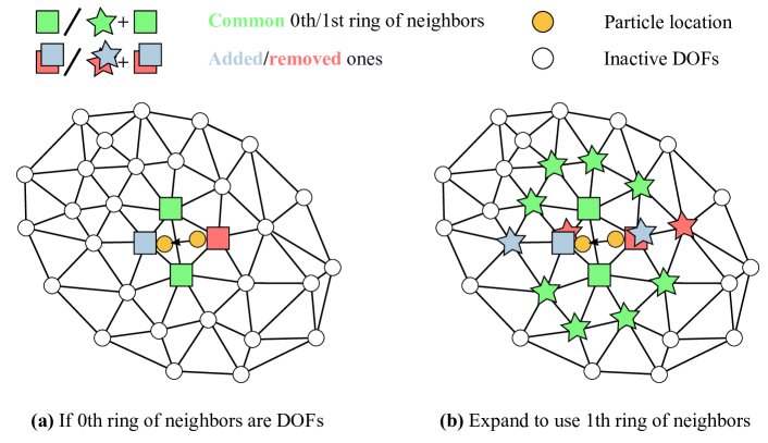
Figure 2: (a) When ${\mathcal{N}}_{p}^{0}$ alone is selected as the active Degrees of Freedom (DOFs), as a particle crosses the cell edge, the DOFs indicated by the blue and red boxes are added or removed, respectively. Consequently, the weights on these DOFs must approach zero to ensure ${\mathcal{C}}^{0}$ continuity, resulting in kernel degeneration along the edge. (b) Advancing to ${\mathcal{C}}^{1}$ addresses this issue by incorporating a sufficient number of DOFs to fully encompass the particles.

Ring Level Selection for Nearby Nodes

When a specific level of ring neighbors is chosen as the nearby nodal degrees of freedom, a natural question arises: What is the minimum number of rings required to satisfy the desired properties of the MPM kernel? Assume ${\mathcal{N}}_{p}^{0}$ is selected, meaning the particle only affects the vertices in the cell where it currently resides, and at least ${\mathcal{C}}^{0}$ continuity is required for the kernel. This scenario leads to the kernel degenerating, which is characterized by the kernel affecting merely the shared edge in 2D or the shared face in 3D when the particle transitions across cell boundaries, as depicted in Figure 2a. Conversely, opting for 1-ring neighbors, ${\mathcal{N}}_{p}^{1}$, effectively circumvents this issue, ensuring a non-degenerate kernel interaction as illustrated in Figure 2b.

Computing the Weights

For conciseness and consistency, we will omit the function arguments and subscripts, such as ${\bm{x}}$ and $i$ in (21). Instead, since we project onto the mesh vertex $v$, we will hereafter use the subscript $v$ and obtain the following rewritten form of (21):

$$\begin{bmatrix}\hat{u}_{p}\\ \nabla\hat{u}_{p}\\ \end{bmatrix}={\bm{M}}_{vp}^{-1}{\bm{Q}}_{vp}^{T}{\bm{D}}_{vp}{\bm{u}}_{vp},$$ (22)

where ${\bm{u}}_{vp}=\left[u_{v_{1}},\dots,u_{v_{n}}\right]^{T}$ is the stacked vertex values with $v_{i}\in{\mathcal{N}}_{p}^{1}$, $i\in[1,~{}n]$ and the matrix ${\bm{M}}_{vp}={\bm{Q}}_{vp}^{T}{\bm{D}}_{vp}{\bm{Q}}_{vp}$ with stacked vertex basis ${\bm{Q}}_{vp}=\left[{\bm{P}}({\bm{x}}_{v_{1}}-{\bm{x}}_{p}),\dots,{\bm{P}}({\bm{x}}_{v_{n}}-{\bm{x}}_{p})\right]^{T}$ and diagonal sample weighting matrix ${\bm{D}}_{vp}$ such that ${\bm{D}}_{pv,i,i}=d_{vp}=d({\bm{x}}_{v_{1}}-{\bm{x}}_{p})$, where $d$ is chosen to be a B-spline function.

2.3.3 Required Properties for the Transfer Kernel

Despite implementing a broader interpolation kernel, the reconstruction method described in Section 2.3.2 is not directly applicable as it still suffers from cell crossing errors. To grasp this problem, consider the essential desirable properties for an MPM kernel:

1. The kernel must be a non-negative partition of unity. This means that the sum of the kernel weights for all nearby vertices to a particle should equal 1; i.e., $\sum_{v\in{\mathcal{N}}_{p}^{1}}w_{v}=1$, with each individual weight $w_{v}\geq 0,\forall v\in{\mathcal{N}}_{p}^{1}$.

2. There should be a continuous reconstruction of both the function value and gradient as the particle transitions across the cell boundary.

Methods such as B-spline MPM and GIMP are specifically designed to fulfill these requirements. With MLS-MPM, the partition of unity is inherently assured by the characteristics of MLS [47]. The non-negativity of this partition additionally depends on preventing sample degeneration, a requirement met in MLS-MPM due to its use of uniform background nodes. Furthermore, MLS-MPM ensures continuous reconstruction by utilizing a B-spline for sample weighting, which provides ${\mathcal{C}}^{1}$ continuity.

A key insight from MLS-MPM is that whenever a grid node is added or removed from the nearby node set, its B-spline weighting function also smoothly approaches zero, ensuring its influence on the assembly of ${\bm{M}}$ and ${\bm{Q}}$ in (21) is infinitesimal and, hence, the continuity of the reconstruction. However, since our method determines nearby vertices based on the ring of neighbors rather than proximity, a uniform sample weighting function cannot guarantee diminishing influence for the added or removed vertices. Consequently, the abrupt changes in influence of these vertices during the MLS assembly yield discontinuous reconstruction. This issue will be addressed in the next section.

2.3.4 Remedying Discontinuous Reconstruction Across the Cell Boundary

To mitigate the abrupt influence changes from vertices being added or removed during cell crossings, an intuitive solution is to diminish their impact on the MLS assembly. This can be accomplished by adjusting the kernel to predominantly rely on vertices that remain common before and after crossing the cell boundary. To achieve this, we modify any initial sample weighting function $d_{vp}$ by incorporating a smooth diminishing function $\eta_{vp}$; i.e., $d_{vp}\leftarrow\eta_{vp}d_{vp}$. Here, $\eta_{vp}$ approaches zero for vertices that are added or removed from ${\mathcal{N}}_{p}^{1}$ during the cell crossing. A detailed proof of the efficacy of this approach is provided in A.1.

For simplex elements, we design the following $\eta_{vp}$:

$$\eta_{vp}=\sum_{n\in{\mathcal{N}}_{p}^{0}}B_{np}{\bm{A}}_{v,n},$$ (23)

where, for particle $p$, $B_{np}$ represents the barycentric weight for $n\in{\mathcal{N}}_{p}^{0}$, and ${\bm{A}}$ is the mesh’s adjacency matrix. Geometrically, for a nearby vertex $v\in{\mathcal{N}}_{p}^{1}$, $\eta_{vp}$ denotes the sum of the barycentric weights for all vertices $n\in{\mathcal{N}}_{p}^{0}$ that are directly connected to $v$. Note that $\eta_{vp}=1,~{}\forall v\in{\mathcal{N}}_{p}^{0}$. A.1 proves the claimed diminishing property for this design in the simplex cell.

2.3.5 Verification of the Proposed Kernel

To verify that the proposed method can produce continuous reconstruction, analytical and numerical solutions of the kernels are produced on 1D and 2D meshes, respectively.

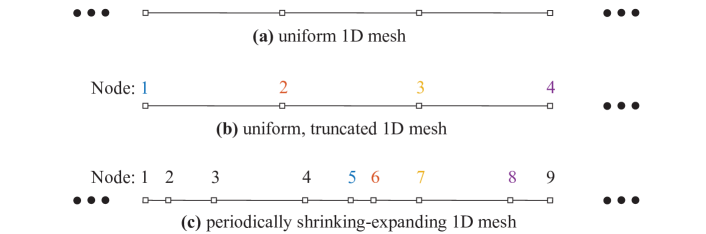
Figure 3: 1D meshes: (a) Uniform. (b) Uniform but truncated. (c) Periodically shrinking/expanding.

For the 1D case, the first basic verification is conducted on a uniform mesh, as the setup in Figure 3a. Figure 4a shows the correct kernel reconstruction with the diminishing function $\eta$, while Figure 4b, as an ablation, shows that the reconstruction can downgrade to being discontinuous even for the simplest uniform mesh, proving the necessity of $\eta$. The detailed setup for this analytical solution is provided in B.

Figure 4: Comparison of kernel values and gradient estimations on a uniform 1D mesh (a) with and (b) without applying the diminishing function.

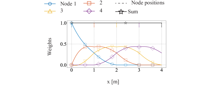
Figure 5: The negative weight for Node 3 (yellow) when the particle is in the boundary cell and there is no extra layer.

Note that the presence of a particle within a boundary element, as depicted in Figure 3b, can lead to a negative weight value for the most interior node. This phenomenon is exemplified by Node 3 in Figure 5, where the kernel degenerates due to the absence of a first ring of neighboring elements on the boundary side during MLS sampling. To remedy the problem of negative kernel values, which can potentially lead to numerical instabilities [48], the introduction of an additional layer of elements beyond the original boundary is recommended as a practical solution.

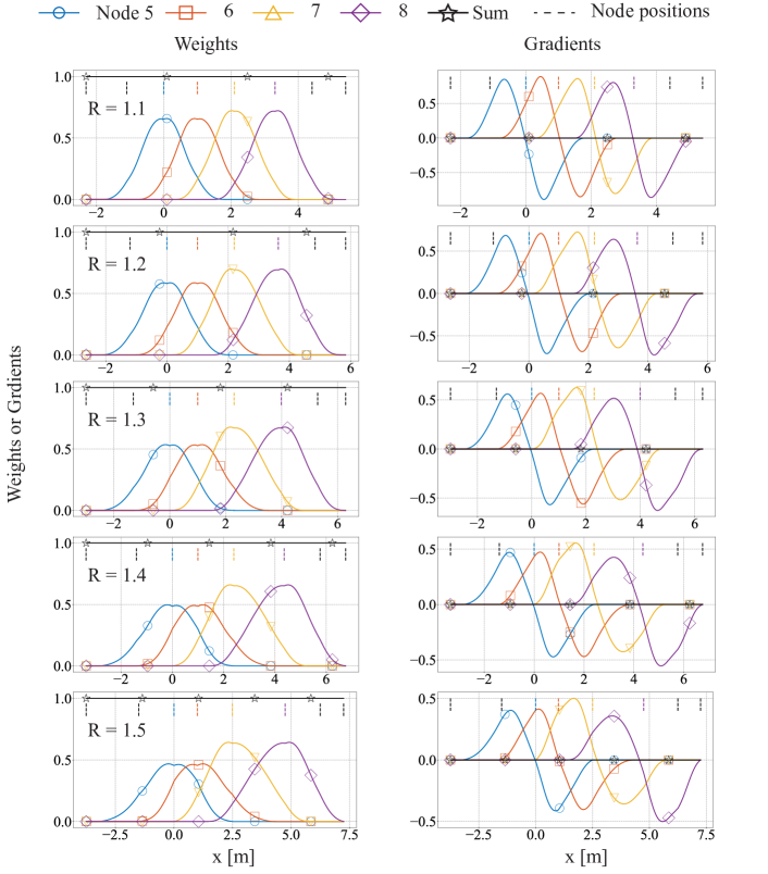
Figure 6: Kernel values (left column) and gradient estimations (right column) on a periodically shrinking/expanding 1D mesh with varying size transition rate $R$.

The next verification is on a periodically shrinking and expanding 1D mesh (Figure 3c). The mesh contains cyclic cell sizes of $[\dots,1,R,R^{2},R,1,\dots]$ designed to mimic the transition between varying resolutions. The size transition ratios tested range from $1.1$ to $1.5$ so as to correspond with the typical transition ratios in FEM analysis. Kernel reconstructions are conducted on Nodes 5, 6, 7, and 8 as they can present a full cycle. As shown in Figure 6, both the kernel and the gradient estimations are piece-wise ${\mathcal{C}}^{1}$.

The final verification and ablation tests were performed on a 2D unstructured mesh featuring “&” shapes. The comparison between scenarios with and without the use of $\eta$, as shown in Figure 7a and Figure 7b respectively, validates the importance of $\eta$ and the effectiveness of the proposed method in managing unstructured meshes.

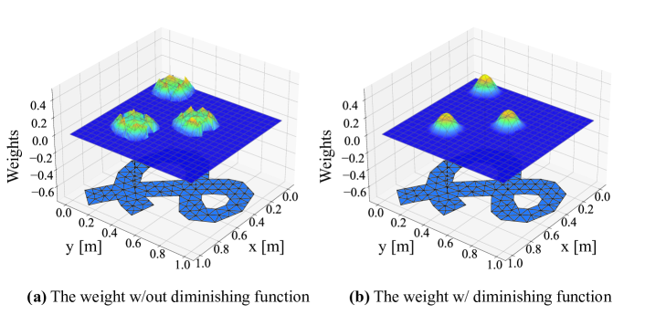
Figure 7: Comparison of the kernel on an unstructured mesh (a) without and (b) with the application of the diminishing function.

3 Experiments and Results

To demonstrate and assess the effectiveness of our approach, particularly its reduced cross-cell error owing to the continuous gradient reconstruction, we have chosen representative test cases from prior related studies. Our benchmarking relies on analytical solutions when feasible, or alternatively, on the standard B-spline MPM at a sufficiently high resolution. All experiments were carried out on a single PC equipped with an Intel^® Core™ i9-10920X CPU.

3.1 1D Vibrating Bar

Figure 8: Setup of the 1D bar vibration test.

Consider the 1D vibration bar problem shown in Figure 8a [49]. The left end of the bar is fixed and the right has a sliding condition in the $x$ direction. The physical properties of the bar are: $E=100$ Pa, $\nu=0$, $L=25$ m, and $\rho=1$ kg/m³. The initial velocity conditions are $\dot{u}(x,t=0)=v_{0}\sin\left(\beta_{1}x\right)$ with $\beta_{1}=\frac{\pi}{2L}$.

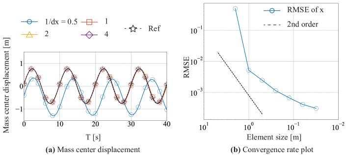
Figure 9: Plots of (a) the center of mass displacement of the bar and (b) convergence rate of the RMSE of particle displacements.

The analytical expression of the center of mass in this problem is

$$x(t)_{CM}=\frac{L}{2}+\frac{v_{0}}{\beta_{1}L\omega_{1}}\sin\left(\omega_{1}t\right),$$ (24)

and

$$\dot{u}(t)_{CM}=\frac{v_{0}}{\beta_{1}L}\cos\left(\omega_{1}t\right),$$ (25)

with $\omega_{1}=\beta_{1}\sqrt{E/\rho}$.

The original experiments in [49] included two velocity settings: $v_{0}=0.1$ m/s and $v_{0}=0.75$ m/s. The lower velocity setting, $v_{0}=0.1$ m/s, was utilized solely for validation against the linear kernel MPM, as it does not involve cell crossings. Here, we focus on the higher-velocity setting to assess the effectiveness of UMLS-MPM in addressing cell-crossing errors.

Figure 9 presents the convergence rate of UMLS-MPM with grid refinement. Specifically, Figure 9a shows that, with the exception of the coarsest resolution $dx=2$ m, UMLS-MPM consistently achieves high accuracy, with a maximum root mean square error (RMSE) of $0.554\%$ in particle displacements. Figure 9b indicates that the convergence rate is approximately second order on coarser grids, but it starts to level off on finer grids due to mounting temporal errors, aligning with established MPM theory [50].

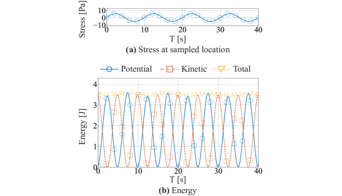
Figure 10: Plots of (a) the stress at the sampled particle closest to $[17.5,0.5]$ and (b) the system energy.

Figure 10a displays the stress profile for a particle located at $x_{0}=12.75$ m, which undergoes the most frequent cell crossings during its vibrational motion. The outcomes achieved with UMLS-MPM showcase a remarkable level of smoothness and precision. Figure 10b illustrates the energy dynamics for the entire system, revealing that the system’s energy is largely conserved throughout the simulation, with only slight fluctuations. These findings collectively underscore the robustness and precision of UMLS-MPM in managing intense cell crossings by particles.

3.2 2D Collision Disks

Figure 11: 2D collision disks: (a) Problem setup. (b)–(d) Snapshots of the simulation at 1.5s, 2.0s, and 2.5s.

Next, we considered the problem of two colliding elastic disks shown in Figure 11a [49]. The physical properties of the disks are: $E=1000$ Pa, $\nu=0.3$, $\rho=1000$ kg/m³, and ${\bm{v}}=\pm(0.1,0.1)$ m/s for the left and right disks, respectively. Each disk was discretized with $462$ material points using the triangle mesh of a disk. The background mesh was generated using Delaunay triangulation with a target element size of $0.025$ m. We plot key snapshots of the simulation in Figure 11b–d, with the impact at $1.5$ s, total retardation right before $2.0$ s, and rebounding separation right before $2.5$ s.

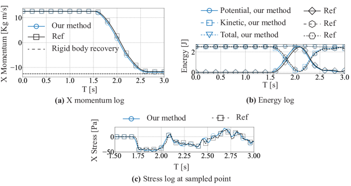
Figure 12: Plots of (a) the momentum in the $x$-direction of the left disk, (b) the energies of the system, and (c) the stress at the sampled particle closest to the center of the left disk.

Quantitative results for the collision disks are presented in Figure 12. In Figure 12a, a comparison of momentum recovery during collision between UMLS-MPM and the B-spline MPM with sufficiently high resolution is shown. While a perfect momentum recovery, such as that in the rigid collision (dashed gray line in Figure 12a), is not expected, UMLS-MPM approaches this limit effectively. Similarly, Figure 12b displays the kinetic energy recovery during the collision. The results indicate that UMLS-MPM effectively preserves the system energy. Figure 12c illustrates the stress log at the center particle of the left disk. The results align perfectly with the reference, but only for negligible fluctuations, showing that UMLS-MPM does not generate spurious stress oscillations either from the collision or cell crossings.

3.3 2D Cantilever With Rotations

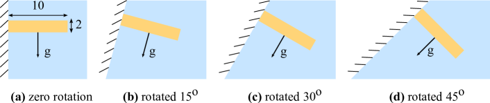
Figure 13: 2D cantilever problem under different rotation angles: (a) $0\text{\,}\mathrm{\SIUnitSymbolDegree}$, (b) $15\text{\,}\mathrm{\SIUnitSymbolDegree}$, (c) $30\text{\,}\mathrm{\SIUnitSymbolDegree}$, and (d) $45\text{\,}\mathrm{\SIUnitSymbolDegree}$.

Although an unstructured mesh offers the adaptability to match any boundary shape, the cell orientation, or a different tessellation, can potentially affect accuracy. To illustrate the precision of our method under various rotation angles, we examined the case of a cantilever under its own weight, as shown in Figure 13a [49]. The cantilever’s physical characteristics are as follows: length $l=10$ m, height $h=2$ m, gravitational acceleration $g=9.81$ m/s², Young’s modulus $E=100000$ Pa, Poisson’s ratio $\nu=0.29$, and density $\rho=2$ kg/m³. The cantilever was discretized with uniformly spaced particles in both directions. We created the background mesh using Delaunay triangulation, aiming for an element size of $0.5$ m. Additionally, we rotated the mesh of the cantilever by angles of $15^{\circ}$, $30^{\circ}$, and $45^{\circ}$ to showcase the resilience of our method to rotation, as depicted in Figure 13b–d.

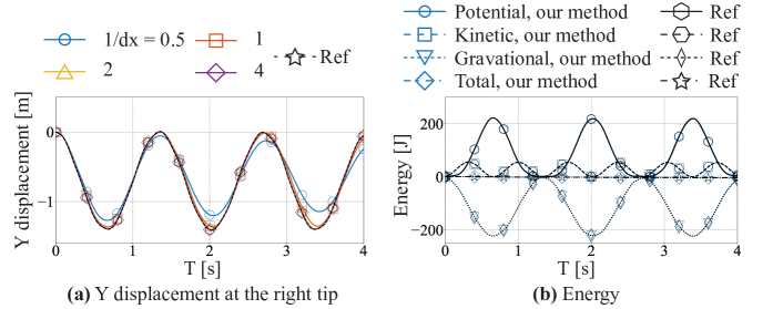
Figure 14: Plots of (a) the displacement in the $y$-direction at the right tip of the cantilever and (b) the energies of the system.

Figure 14a illustrates the spatial convergence of the $y$-displacement at the right tip of the cantilever beam under grid refinement. Notably, except for the coarse resolutions of $dx=2$ m and $dx=1$ m, errors for all finer resolutions are negligible. Therefore, a resolution of $dx=0.5$ m was employed to ensure sufficient accuracy for all subsequent plots in this experiment. Figure 14b demonstrates that UMLS-MPM effectively conserves energy, aligning with the reference B-spline MPM.

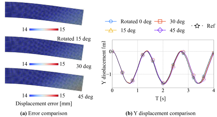
Figure 15: (a) Snapshots of the cantilever with different initial rotating angles. (b) Comparison of the displacement in the $y$-direction at the right tip of the cantilever.

Figure 15a shows snapshots of the cantilever with different initial mesh rotation angles. The results indicate that UMLS-MPM is robust under mesh rotation with only minor visible errors. Figure 15b quantitatively compares the $y$-displacement at the right tip. The results align well overall with both zero rotation and the reference, with errors of $1.27\%$, $2.18\%$, and $4.72\%$ for $15^{\circ}$, $30^{\circ}$, and $45^{\circ}$ rotation, respectively.

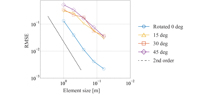
Figure 16: Convergence plot of the RMSE of particle displacements.

The convergence rate of UMLS-MPM is demonstrated in Figure 16. The results indicate that for cases with zero rotation, the convergence rate is second order. While the RMSE increases slightly for cases with mesh rotation, it still remains in the magnitude of $1E-2$, and the convergence rate remains near second order. These combined results demonstrate the robustness and accuracy of UMLS-MPM under mesh rotation.

3.4 3D Slope Failure

Next, the performance of the proposed approach was investigated when dealing with material behavior involving plasticity. To this end, we simulated failure of a 3D slope comprosed of sensitive clay. The problem geometry was adopted from [51] and is illustrated in Figure 17. Here, the bottom boundary of the slope is fixed and the three lateral sides are supported with rollers. To model the elastoplastic behavior of the sensitive clay in an undrained condition, a combination of Hencky elasticity and J2 plasticity with softening was used. The softening behavior is governed by the following exponential form: $\kappa=(\kappa_{p}-\kappa_{r})e^{-\eta\varepsilon_{q}^{p}}+\kappa_{r}$, where $\kappa$, $\kappa_{p}$, and $\kappa_{r}$ denote the yield strength, the peak strength, and the residual strength, respectively, $\varepsilon_{q}^{p}$ denotes the equivalent plastic strain, and $\eta$ is a softening parameter. The specific parameters were adopted from [51]. They are a Young’s modulus of $E=25$ MPa, a Poisson’s ratio of $\nu=0.499$, a peak strength of $\kappa_{p}=40.82$ kPa, a residual strength of $\kappa_{r}=2.45$ kPa, and a softening parameter of $\eta=5$. The assigned soil density is $\rho=2.15$ t/m³.

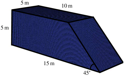
Figure 17: Problem geometry of the 3D slope failure (adapted from [51]).

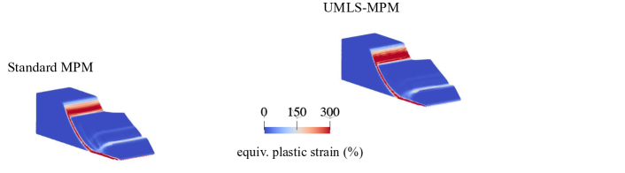
(a) $t=1.5$ s

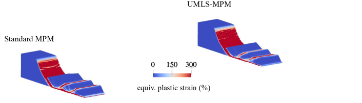
(b) $t=2.5$ s

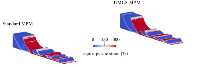
(c) $t=3.5$ s

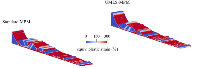
(d) $t=5.5$ s

Figure 18: Snapshots of the solutions from the UMLS-MPM and the standard MPM with quadratic B-splines basis functions in Zhao et al. [51]. Particles are colored based on the equivalent plastic strain.

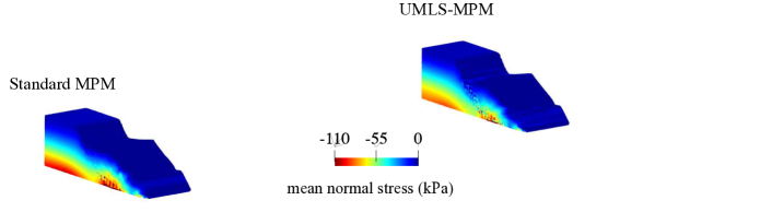
(a) $t=1.5$ s

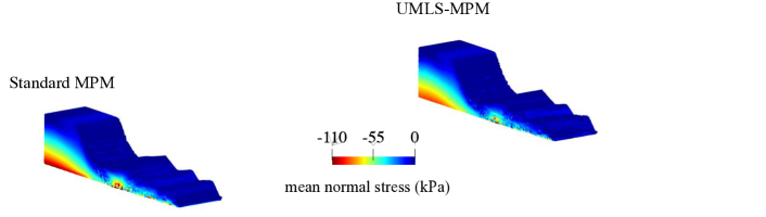
(b) $t=2.5$ s

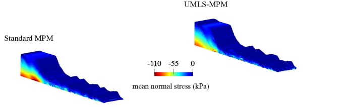
(c) $t=3.5$ s

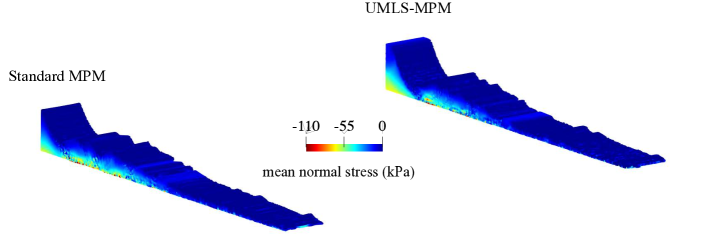
(d) $t=5.5$ s

Figure 19: Snapshots of the solutions from the UMLS-MPM and the standard MPM with quadratic B-splines basis functions in Zhao et al. [51]. Particles are colored based on the mean normal stress.

The space was discretized using Delaunay triangulation with the shortest edge length of 0.2 m. The material points were initialized with a spacing of 0.1 m in each direction, amounting to 311,250 material points in the initial slope region. Note that the spatial discretization aligns with the one used in [51] in terms of both the shortest edge length of the background element and the number of material points. Also, the $\bar{\bm{F}}$ approach proposed in [51] was utilized to circumvent volumetric locking that UMLS-MPM solutions encounter when simulating a large number of particles of incompressible materials. As a reference to verify the correctness of the proposed formulation, the $\bar{\bm{F}}$ solution in [51] was used.

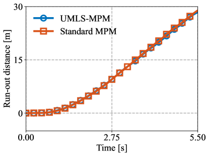
Figure 20: Time evolutions of the run-out distance from UMLS-MPM and the standard MPM.

Figures 18 and 19 show the snapshots of the slope simulated by the standard and UMLS-MPM, where particles are colored by the equivalent plastic strain and mean normal stress, respectively. We can see that UMLS-MPM effectively captures the retrogressive failure pattern of slopes made of sensitive clay. Also, in terms of equivalent plastic strain fields and mean normal stress fields, we observe a strong similarity between the UMLS-MPM solution and the reference solution from [51].

For a further quantitative comparison, Figure 20 presents the time evolutions of the run-out distance—a measure of the farthest movement of the sliding mass. Observe that the distances in the standard and UMLS-MPM solutions are remarkably similar. Taken together, these findings confirm that the proposed method performs similarly to the standard MPM.

3.5 3D Elastic Object Expansion in a Spherical Container

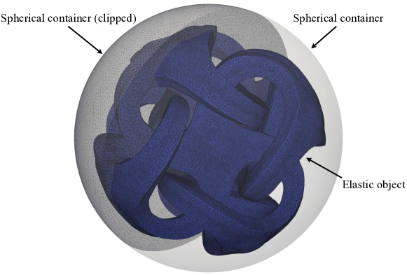
Figure 21: Problem setting of the 3D elastic object expansion in a spherical container.

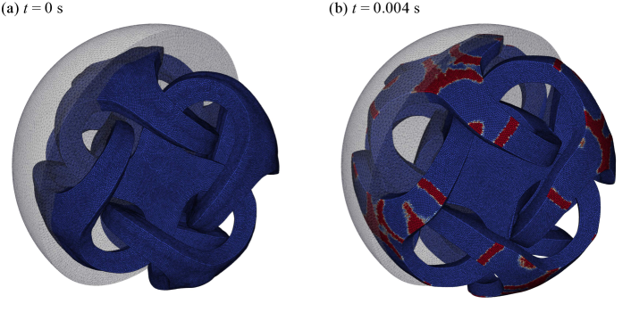
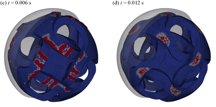
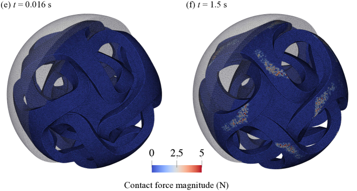
Figure 22: Snapshots from the UMLS-MPM solutions in which particles are colored based on the magnitude of the contact force.

Finally, we examined the performance of UMLS-MPM in problems involving complex boundary geometry. In this problem, the standard MPM with a structured grid may be challenged to impose conforming boundary conditions. Hence, a collision between an elastic body with a spherical container was considered and simulated.

The geometry of the problem, as demonstrated in Figure 21, involves an elastic object in the shape of a Metatron, which is located at the center of a spherical container (with a radius of 0.5 m). The object is initially compressed isotropically (with an initial deformation gradient of $\bm{F}=0.75\bm{I}$), storing non-zero elastic potential energy. At the onset of the simulation, the stored elastic energy is released, causing the object to expand and collide with the spherical container’s boundary. To capture the elastic behavior of the object, a Neohooken elasticity was adopted with a Young’s modulus of 3.3 MPa and a Poisson’s ratio of $\nu=0.49$. The elastic object was discretized using a significant number of material points (2,392,177) for high-fidelity simulation. Also, the spherical container was discretized using 2,178,129 tetrahedral elements, each with an average edge length of $h=0.025$ m. Note that to avoid negative kernel values at boundary nodes, an extra layer of elements was added outside the original boundary, as discussed in Section 2.3.5.

To consider the frictional collision between the elastic object and the container boundary, a barrier approach [52] was adopted, ensuring that the elastic object does not penetrate the boundary. Contact forces are applied when the distance between a material point and the boundary is below a specific value $\hat{d}$, which was chosen to be a quarter of $h$ for sufficient accuracy. Also, a friction coefficient of $\mu=0.5$ was introduced to stop the sliding of the elastic object in the later stages. The simulation ran with a time increment of $\Delta t=6.16\times 10^{-5}$ s until $t=1.5$ s.

Figure 22 presents six snapshots simulated with UMLS-MPM, where the particles are colored based on the magnitude of the contact force. The dynamic behavior of the object at various stages is well captured, including the initial expansion stage (a), the first collision stage (b–d), the rebounding stage (e), and the final static stage (f). Overall, the UMLS-MPM effectively handles complex geometry with a conformal discretization, which is critical for simulating a wide range of interactions between deformable objects and complex boundaries.

4 Conclusion, Limitations, and Future Work

This study has extended the Moving Least Square Material Point Method (UMLS-MPM) to encompass general tessellations within both 2D and 3D meshes. This advance has been achieved through the multiplication of a diminishing function to the MLS sample weights. Analytically proved, the approach ensures continuous kernel reconstruction and provides a sound foundation for high-order MPM on any unstructured mesh types. Several numerical experiments in both 2D and 3D domains have shown the method’s effectiveness in high-order convergence and the elimination of cell-crossing errors.

However, the proposed method still has limitations. To ensure the MLS solution does not degenerate, there are quality requirements on the surrounding vertices of the particle, which pose challenges, especially in meshes with sharp resolution transitions or poor quality. Another trigger for degeneracy is the lack of surrounding samples on one side; for example, when the particle is near the domain boundary. While this issue was mitigated in our last experiment by drawing an extra layer of vertices, their automatic creation via an algorithm would be an improvement. Additionally, the selection of sample weights also poses a challenge. We used a B-spline function with a fixed unit support length equaling the maximum element size to ensure that the first ring of neighbors is reserved even in the coarsest area. However, this strategy leads to more uniform sample weights in finer regions, blurring the kernel. A potential solution can be to incorporate a sizing field within the mesh to dynamically adjust the sample weight function.

From an application standpoint, exploring the integration between the Material Point Method (MPM) and gas or fluid simulations via the Finite Volume Method (FVM) presents significant potential [21, 53]. Furthermore, recent advances have seen learning MPM or other mesh-based simulations using graph neural networks, accelerating the inferences [54, 55, 56]. Our kernel construction suggests a potentially novel learning paradigm for MPM on unstructured meshes, which is similar to embedding both kernel and mesh information into the network’s channel [57, 58].

Appendix A Proofs for the Continuous Reconstructions

A.1 Proofs

For conciseness, we drop the subscripts _vp in the following proofs. We start by assuming there exists a smooth, diminishing function $\eta$ for the nodes added or removed from the set of nearby nodes ${\mathcal{N}}^{1}$ when a particle crosses the boundary of a cell. Under this assumption, we can prove that our kernel value and gradient estimation is continuous across the boundary. We present the proof in 2D when a particle crosses an edge; the extension to 3D and other crossing cases is straightforward. Then, we prove that the proposed function in (23) is locally diminishing for ${\mathcal{N}}_{a,r}^{1}$ when the particle crosses the edge.

Proposition 1.

Our kernel value and gradient estimation is continuous across cell boundaries.

Proof.

Let ${\mathcal{N}}_{o,n}^{1}$ be the sets of nearby nodes before/after the particle $p$ crosses the common edge between the old/new cells ${\mathcal{N}}_{o,n}^{0}$. Here, the subscripts ${o,n}$ denote the old/new cell, respectively, and the superscripts ${0,1}$ indicate the ring-0/1 neighbors of the cell, respectively. Let ${\bm{x}}_{p}^{o,n}$ be the position of particle $p$ before/after the crossing and $||{\bm{x}}_{p}^{n}-{\bm{x}}_{p}^{o}||={\mathcal{O}}(\epsilon)$. Define the common node set ${\mathcal{N}}_{c}^{1}={\mathcal{N}}_{o}^{1}\cap{\mathcal{N}}_{n}^{1}$, the added node set ${\mathcal{N}}_{a}^{1}={\mathcal{N}}_{n}^{1}\setminus{\mathcal{N}}_{c}^{1}$, and the removed node set ${\mathcal{N}}_{r}^{1}={\mathcal{N}}_{o}^{1}\setminus{\mathcal{N}}_{c}^{1}$. Since $\eta$ is locally diminishing for $v\in{\mathcal{N}}_{a,r}^{1}$, we have a positive value $K_{1}$ such that $\eta={\mathcal{O}}(K_{1}\epsilon)={\mathcal{O}}(\epsilon)$. The pertubation for the assembled matrix ${\bm{M}}$ before/after the particle $p$ crosses an edge is

$$\delta{\bm{M}}=\sum_{v\in{\mathcal{N}}_{c}^{1}}\delta(\eta d{\bm{P}}{\bm{P}}^{T})+\sum_{v\in{\mathcal{N}}_{a}^{1}}\eta d{\bm{P}}{\bm{P}}^{T}-\sum_{v\in{\mathcal{N}}_{r}^{1}}\eta d{\bm{P}}{\bm{P}}^{T},$$ (26)

where the first term is continuous by construction since every factor is smooth; i.e., $||\delta(\eta d{\bm{P}}{\bm{P}}^{T})||={\mathcal{O}}(\epsilon)$. For the second and third terms, since $\eta={\mathcal{O}}(\epsilon)$, we have

$$||\delta{\bm{M}}|| \leq\sum_{v\in{\mathcal{N}}_{c}^{1}}||\delta(\eta d{\bm{P}}{\bm{P}}^{T})||+\sum_{v\in{\mathcal{N}}_{a}^{1}}||\eta d{\bm{P}}{\bm{P}}^{T}||+\sum_{v\in{\mathcal{N}}_{r}^{1}}||\eta d{\bm{P}}{\bm{P}}^{T}||$$ (27)

$$\leq\biggl{[}|{\mathcal{N}}_{c}^{1}|+\left(|{\mathcal{N}}_{a}^{1}|+|{\mathcal{N}}_{r}^{1}|\right)\max_{v\in{\mathcal{N}}^{1}_{a,r}}||d{\bm{P}}{\bm{P}}^{T}||\biggr{]}{\mathcal{O}}(\epsilon)$$

$$={\mathcal{O}}(|{\mathcal{N}}^{1}|h^{2}\epsilon)$$

$$={\mathcal{O}}(\epsilon).$$

Here, as long as the mesh has a reasonably good quality, $|{\mathcal{N}}^{1}|$ is finite and small; i.e., there is a finite and small amount of ring-1 neighbors. Also, $h$, a constant, is the support radius of the kernel, outside of which the weight is zero. In all, both $|{\mathcal{N}}^{1}|$ and $h$ can be omitted in the analysis.

The perturbation of the inverse matrix is given by

$$||\delta{\bm{M}}^{-1}|| =||({\bm{M}}+\delta{\bm{M}})^{-1}-{\bm{M}}^{-1}||$$ (28)

$$=||{\bm{M}}^{-1}-{\bm{M}}^{-1}\delta{\bm{M}}{\bm{M}}^{-1}+{\mathcal{O}}(||\delta{\bm{M}}||^{2})-{\bm{M}}^{-1}||$$

$$=||{\bm{M}}^{-1}\delta{\bm{M}}{\bm{M}}^{-1}+{\mathcal{O}}(\epsilon^{2})||$$

$$\leq||{\bm{M}}^{-1}\delta{\bm{M}}{\bm{M}}^{-1}||+{\mathcal{O}}(\epsilon^{2})$$

$$\leq||{\bm{M}}^{-1}||^{2}\cdot||\delta{\bm{M}}||+{\mathcal{O}}(\epsilon^{2})$$

$$=\frac{||\delta{\bm{M}}||}{\sigma({\bm{M}})^{2}_{\min}}+{\mathcal{O}}(\epsilon^{2})$$

$$={\mathcal{O}}\left(\frac{\epsilon}{\sigma({\bm{M}})^{2}_{\min}}\right)+{\mathcal{O}}(\epsilon^{2})$$

$$={\mathcal{O}}\left(\frac{\epsilon}{\sigma({\bm{M}})^{2}_{\min}}\right),$$

where $\sigma({\bm{M}})_{\min}$ is the minimum singular value of ${\bm{M}}$.

Similarly, for the perturbation in the assembled vector ${\bm{Q}}^{T}{\bm{D}}{\bm{u}}$ before/after the particle crossing is

$$||\delta\left({\bm{Q}}^{T}{\bm{D}}{\bm{u}}\right)|| =||\sum_{v\in{\mathcal{N}}_{c}^{1}}\delta(\eta du{\bm{P}})+\sum_{v\in{\mathcal{N}}_{a}^{1}}\eta du{\bm{P}}-\sum_{v\in{\mathcal{N}}_{r}^{1}}\eta du{\bm{P}}||$$ (29)

$$\leq\sum_{v\in{\mathcal{N}}_{c}^{1}}||\delta(\eta du{\bm{P}})||+\sum_{v\in{\mathcal{N}}_{a}^{1}}||\eta du{\bm{P}}||+\sum_{v\in{\mathcal{N}}_{r}^{1}}||\eta du{\bm{P}}||$$

$$\leq\left[|{\mathcal{N}}_{c}^{1}|+\left(|{\mathcal{N}}_{a}^{1}|+|{\mathcal{N}}_{r}^{1}|\right)\max_{v\in{\mathcal{N}}^{1}_{a,r}}||du{\bm{P}}||\right]{\mathcal{O}}(\epsilon)$$

$$={\mathcal{O}}(|{\mathcal{N}}^{1}|h\epsilon)$$

$$={\mathcal{O}}(\epsilon).$$

Furthermore, we can establish the following bound for the assembled vector ${\bm{Q}}^{T}{\bm{D}}{\bm{u}}$:

$$||{\bm{Q}}^{T}{\bm{D}}{\bm{u}}|| =||\sum_{v\in{\mathcal{N}}^{1}}\eta du{\bm{P}}||$$ (30)

$$\leq|{\mathcal{N}}^{1}|\cdot\max_{v\in{\mathcal{N}}^{1}}||\eta du{\bm{P}}||$$

$$={\mathcal{O}}(|{\mathcal{N}}^{1}|h)$$

$$={\mathcal{O}}(1).$$

Finally, the perturbation for $\left[\hat{u}_{p},\nabla\hat{u}_{p}^{T}\right]^{T}$ from (22) is

$$\left[\hat{u}_{p},\nabla\hat{u}_{p}^{T}\right]^{T} =||\delta({\bm{M}}^{-1}{\bm{Q}}^{T}{\bm{D}}{\bm{u}})||$$ (31)

$$=||\delta{\bm{M}}^{-1}{\bm{Q}}^{T}{\bm{D}}{\bm{u}}+{\bm{M}}^{-1}\delta\left({\bm{Q}}^{T}{\bm{D}}{\bm{u}}\right)||$$

$$\leq||\delta{\bm{M}}^{-1}{\bm{Q}}^{T}{\bm{D}}{\bm{u}}||+||{\bm{M}}^{-1}\delta\left({\bm{Q}}^{T}{\bm{D}}{\bm{u}}\right)||$$

$$\leq||\delta{\bm{M}}^{-1}||\cdot||{\bm{Q}}^{T}{\bm{D}}{\bm{u}}||+||{\bm{M}}^{-1}||\cdot||\delta\left({\bm{Q}}^{T}{\bm{D}}{\bm{u}}\right)||$$

$$={\mathcal{O}}\left(\left(\frac{1}{\sigma({\bm{M}})^{2}_{\min}}+\frac{1}{\sigma({\bm{M}})_{\min}}\right)\epsilon\right).$$

In the incomplete singular value decomposition of ${\bm{M}}$, the singular values will always be non-negative. And if the surrounding nodes are not degenerate, the minimum singular value $\sigma({\bm{M}})_{\min}$ will always be positive and the condition number of ${\bm{M}}$ is bounded. Therefore, as long as the mesh is of reasonably good quality, both the function value and gradient estimation is ${\mathcal{C}}^{0}$ across the boundary. ∎

Proposition 2.

The function $\eta$ in (23) is locally diminishing for $\forall v\in{\mathcal{N}}_{a,r}^{1}$.

Proof.

Formally, we need to prove that for any $v\in{\mathcal{N}}_{a,r}^{1}$, when ${\bm{x}}_{p}$ is crossing the edge of a triangle and $||{\bm{x}}_{p}^{n}-{\bm{x}}_{p}^{o}||={\mathcal{O}}(\epsilon)$, the smoothing function $\eta={\mathcal{O}}(\epsilon)$.

Denote the edge that the particle is crossing as $e$ and the portion of $||{\bm{x}}_{p}^{n}-{\bm{x}}_{p}^{o}||$ in the new/old cell as $L^{n,o}$. Trivially,

$$L^{n,o} \leq L^{n}+L^{o}$$ (32)

$$=||{\bm{x}}_{p}^{n}-{\bm{x}}_{p}^{o}||$$

$$={\mathcal{O}}(\epsilon).$$

Then, let the far-away node not on the edge but in the new/old cell be $v_{far}$ (i.e., $v_{far}^{n,o}\notin e\,\land\,v_{far}^{n,o}\in{\mathcal{N}}_{o,n}^{0}$) and the height from a node $v$ to an edge $e$ be $H(v,e)$. Since the height is orthogonal to the edge, we have $H({\bm{x}}_{p}^{n,o},e)\leq L^{n,o}={\mathcal{O}}(\epsilon)$. Consider the barycentric coordinate contributed by the far-away node, in the new/old cell respectively, for ${\bm{x}}_{p}$:

$$B^{n,o}_{v_{far}} =\frac{H({\bm{x}}_{p}^{n,o},e)\cdot||e||}{H(v_{far}^{n,o},e)\cdot||e||}$$ (33)

$$=\frac{H({\bm{x}}_{p}^{n,o},e)}{H(v_{far}^{n,o},e)}$$

$$={\mathcal{O}}(\frac{\epsilon}{H(v_{far}^{n,o},e)})$$

$$={\mathcal{O}}(\epsilon).$$

Figure 23: A visual representation of the notations used to prove that $\eta$ diminishes locally, as described in (33), for every vertex $v$ within the first ring of neighbors, ${\mathcal{N}}^{1}_{a,r}$. The dashed line denotes the perpendicular height from a given position to the shared edge. Dotted lines are drawn to construct a triangle between the point ${\bm{x}}_{p}$ and the edge, facilitating the computation of the barycentric coordinates.

Finally, if a node is added/removed during the particle crossing (i.e., $v\in{\mathcal{N}}_{a,r}^{1}$), this means that $v$ is only connected to the far-away nodes $v_{far}^{n,o}$ but not to the edge $e$; i.e., ${A}_{v,v_{far}^{n,o}}=1,\forall v\in{\mathcal{N}}^{1}_{a,r}$, otherwise ${A}_{v,n}=0,\forall n\in e\land\forall v\in{\mathcal{N}}^{1}_{a,r}$. Hence,

$$\eta =\sum_{n\in{\mathcal{N}}^{0}}B_{n}{A}_{v,n}$$ (34)

$$=B^{n,o}_{v_{far}}{A}_{v,v_{far}^{n,o}}+\sum_{n\in e}B_{n}{A}_{v,n}$$

$$=B^{n,o}_{v_{far}}\cdot 1+\sum_{n\in e}B_{n}\cdot 0$$

$$=B^{n,o}_{v_{far}}$$

$$={\mathcal{O}}(\epsilon),\quad\forall v\in{\mathcal{N}}^{1}_{a,r}.$$

This concludes the proof. ∎

Appendix B Settings and Analytical Solutions for the Verification Experiments of the Continuous Reconstructions

This section presents the detailed setup and analytical solutions for the 1D verification experiments on a uniform 1D mesh in Section 2.3.5. The kernel value is denoted as $f$ and the gradient estimation is denoted as $g$, respectively. For the uniform 1D mesh, each cell has a length of $1$, and the unit support length for the B-spline used for the sample weights is also $1$. The analytical solution for the uniform 1D mesh, obtained using Mathematica 2023, is as follows:

$$\begin{array}[]{cc}f=&\begin{cases}\frac{0.25(0.5\,-x)^{2}x}{x^{5}-6x^{4}+13.5x^{3}-13.75x^{2}+6.3125x-0.5625},&0.5<x\leq 1\\ \frac{-x^{6}+5x^{5}-9.5x^{4}+8.5x^{3}-3.3125x^{2}+0.3125x+0.0625}{-x^{5}+4x^{4}-5.5x^{3}+3.25x^{2}-1.3125x+1.0625},&1<x\leq 1.5\\ \frac{x^{6}-12x^{5}+58.5x^{4}-148.25x^{3}+205.563x^{2}-147.063x+42.25}{x^{5}-11x^{4}+47.5x^{3}-100.25x^{2}+103.313x-41.125},&1.5<x\leq 2\\ \frac{x^{6}-12x^{5}+58.5x^{4}-147.75x^{3}+202.563x^{2}-141.438x+39}{-x^{5}+9x^{4}-31.5x^{3}+53.75x^{2}-45.3125x+16.125},&2<x\leq 2.5\\ \frac{x^{6}-19x^{5}+149.5x^{4}-623.5x^{3}+1453.31x^{2}-1794.19x+915.687}{-x^{5}+16x^{4}-101.5x^{3}+318.75x^{2}-495.313x+304.188},&2.5<x\leq 3\\ \frac{-0.25x^{3}+2.75x^{2}-10.0625x+12.25}{-x^{5}+14x^{4}-77.5x^{3}+212.25x^{2}-288.313x+156.688},&3<x\leq 3.5\\ 0,&\text{Otherwise}\end{cases}\\ \end{array}$$ (35)

$$\begin{array}[]{cc}g=&\begin{cases}-\frac{1(0.5\,-x)^{2}x(x-2)}{x^{5}-6x^{4}+13.5x^{3}-13.75x^{2}+6.3125x-0.5625},&0.5<x\leq 1\\ \frac{-x^{5}+5x^{4}-10.5x^{3}+11.5x^{2}-5.8125x+1.0625}{-x^{5}+4x^{4}-5.5x^{3}+3.25x^{2}-1.3125x+1.0625},&1<x\leq 1.5\\ \frac{-x^{5}+9x^{4}-33.5x^{3}+65.75x^{2}-67.3125x+27.625}{-x^{5}+11x^{4}-47.5x^{3}+100.25x^{2}-103.313x+41.125},&1.5<x\leq 2\\ \frac{-x^{5}+11x^{4}-49.5x^{3}+112.25x^{2}-125.313x+53.625}{x^{5}-9x^{4}+31.5x^{3}-53.75x^{2}+45.3125x-16.125},&2<x\leq 2.5\\ \frac{-x^{5}+15x^{4}-90.5x^{3}+274.5x^{2}-417.813x+254.188}{x^{5}-16x^{4}+101.5x^{3}-318.75x^{2}+495.313x-304.188},&2.5<x\leq 3\\ \frac{x^{4}-13x^{3}+62.25x^{2}-129.5x+98}{-x^{5}+14x^{4}-77.5x^{3}+212.25x^{2}-288.313x+156.688},&3<x\leq 3.5\\ 0,&\text{Otherwise}\end{cases}\\ \end{array}$$ (36)

Appendix C Conservation of the Linear and Affine Momentum When Combined With Affine Particle-in-Cell

Since UMLS-MPM by construction generates a kernel that is the partition of unity and conserves the linear basis [47], i.e.,

$$\sum_{i}w_{ip}^{n} =1,$$

$$\sum_{i}w_{ip}^{n}{\bm{x}}_{i}^{n} ={\bm{x}}_{p}^{n},$$

$$\sum_{i}w_{ip}^{n}({\bm{x}}_{i}^{n}-{\bm{x}}_{p}^{n}) =0,$$

then the system’s total linear and angular momentum will be conserved when combined with the Affine Particle in Cell (APIC) scheme [59, 60]. A simple introduction to APIC is given here for the sake of completeness, while the detailed proof can found in the supplementary document of the original APIC paper [59].

In APIC, mass $m_{p}$, position ${\bm{x}}_{p}$, velocity ${\bm{v}}_{p}$, and an affine matrix ${\bm{B}}_{p}=\sum_{i}w_{ip}v_{i}({\bm{x}}_{i}-{\bm{x}}_{p})^{T}$ are stored and tracked on particles. Then,

Definition 1.

The total linear momentum on grids is

$${\bm{P}}^{tot}_{i}=\sum_{i}m_{i}{\bm{v}}_{i}.$$

Definition 2.

The total linear momentum on particles is

$${\bm{P}}^{tot}_{p}=\sum_{p}m_{p}{\bm{v}}_{p}.$$

Definition 3.

The total angular momentum on grids is

$${\bm{I}}^{tot}_{i}=\sum_{i}{\bm{x}}_{i}\times m_{i}{\bm{v}}_{i}.$$

Definition 4.

The total angular momentum on particles is

$${\bm{I}}^{tot}_{p}=\sum_{p}{\bm{x}}_{p}\times m_{p}{\bm{v}}_{p}+\sum_{p}m_{p}({\bm{B}}_{p})^{T}:\mathbb{\epsilon},$$

where $\mathbb{\epsilon}$ is the Levi-Civita permutation tensor, and for any matrix ${\bm{A}}$, the contraction ${\bm{A}}:\mathbb{\epsilon}=\sum_{\alpha\beta}A_{\alpha\beta}\mathbb{\epsilon}_{\alpha\beta\gamma}$, which is usually used to transition from a cross product into the tensor product ${\bm{u}}\times{\bm{v}}=({\bm{v}}{\bm{u}}^{T})^{T}:\mathbb{\epsilon}$. Also note that for the total angular momentum of the particles: 1) the grid node locations can be perceived as the sample points of a rotating mass centered at the material particle location, and 2) the total angular momentum comprises both that of the center and that of the affine-rotation of the grids around the center.

APIC P2G is given by

$$\begin{split}m_{i}^{n}&=\sum_{p}w_{ip}^{n}m_{p}\\ {\bm{D}}_{p}^{n}&=\sum_{i}w_{ip}^{n}({\bm{x}}_{i}^{n}-{\bm{x}}_{p}^{n})({\bm{x}}_{i}^{n}-{\bm{x}}_{p}^{n})^{T}\\ m_{i}^{n}{\bm{v}}_{i}^{n}&=\sum_{p}w_{ip}^{n}m_{p}({\bm{v}}_{p}^{n}+{\bm{B}}_{p}^{n}({\bm{D}}_{p}^{n})^{-1}({\bm{x}}_{i}^{n}-{\bm{x}}_{p}^{n}))\end{split}$$ (37)

with G2P given by

$$\begin{split}{\bm{v}}_{p}^{n+1}&=\sum_{i}w_{ip}^{n}\tilde{v}_{i}^{n+1}\\ {\bm{B}}_{p}^{n+1}&=\sum_{i}w_{ip}^{n}\tilde{v}_{i}^{n+1}({\bm{x}}_{i}^{n}-{\bm{x}}_{p}^{n})^{T},\end{split}$$ (38)

where the superscript $\tilde{}$ means the intermediate value after the update on grids but before the G2P process.

C.1 Numerical Validation

Figure 24: Setup and snapshots of a rotating elastic square.

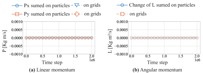
Figure 25: Logs of (a) linear and (b) angular momentum of the rotating cube experiment after $10^{6}$ time steps.

A numerical validation as in [59] is also conducted here to verify these conservations. A square with a side length of $l=0.2$ is discretized with $20\times 20$ particles. The physical properties of the square are as follows: $E=1\times 10^{4}$ Pa, $\nu=0.3$, and $\rho=1.0$ kg/m³. Initially, the square is divided into two halves by a hypothetical vertical line through the middle. The left half is initialized with an upward velocity $\mathbf{v}=(1,0)$ m/s, while the right half is initialized with a downward velocity $\mathbf{v}=(-1,0)$ m/s. The background mesh is generated using Delaunay triangulation with a target element size of $0.01$ m in a $1\times 1$ m² box. The simulation is run for $1\times 10^{6}$ time steps with a time step size of $1\times 10^{-5}$ s.

The proposed conservation is accurately illustrated in Figure 25b–c, with only round-off errors on the order of $1\times 10^{-15}$ and $1\times 10^{-7}$ for the total linear and affine momentum of the system, respectively.

References

- [1] D. Sulsky, S. Zhou, H. L. Schreyer, Application of a particle-in-cell method to solid mechanics, Computer physics communications 87 (1-2) (1995) 236–252.
- [2] J. U. Brackbill, D. B. Kothe, H. M. Ruppel, FLIP: a low-dissipation, particle-in-cell method for fluid flow, Computer Physics Communications 48 (1) (1988) 25–38.
- [3] F. H. Harlow, The particle-in-cell method for numerical solution of problems in fluid dynamics, Tech. rep., Los Alamos Scientific Lab., N. Mex. (1962).
- [4] I. Ionescu, J. E. Guilkey, M. Berzins, R. M. Kirby, J. A. Weiss, Simulation of soft tissue failure using the material point method, Journal of Biomechanical Engineering 128 (2006) 917–924.
- [5] J. E. Guilkey, J. B. Hoying, J. A. Weiss, Computational modeling of multicellular constructs with the material point method, Journal of biomechanics 39 (11) (2006) 2074–2086.
- [6] J. Guilkey, T. Harman, B. Banerjee, An Eulerian–Lagrangian approach for simulating explosions of energetic devices, Computers & structures 85 (11-14) (2007) 660–674.
- [7] S. Ma, X. Zhang, Y. Lian, X. Zhou, Simulation of high explosive explosion using adaptive material point method, Computer Modeling in Engineering and Sciences (CMES) 39 (2) (2009) 101.
- [8] M. A. Homel, R. M. Brannon, J. E. Guilkey, Simulation of shaped-charge jet penetration into drained and undrained sandstone using the material point method with new approaches for constitutive modeling, CIMNE, Barcelona (2014) 676–687.
- [9] G. Klár, T. Gast, A. Pradhana, C. Fu, C. Schroeder, C. Jiang, J. Teran, Drucker-prager elastoplasticity for sand animation, ACM Transactions on Graphics (TOG) 35 (4) (2016) 103.
- [10] A. P. Tampubolon, T. Gast, G. Klár, C. Fu, J. Teran, C. Jiang, K. Museth, Multi-species simulation of porous sand and water mixtures, ACM Transactions on Graphics (TOG) 36 (4) (2017) 105.
- [11] A. Stomakhin, C. Schroeder, L. Chai, J. Teran, A. Selle, A material point method for snow simulation, ACM Transactions on Graphics (TOG) 32 (4) (2013) 102.
- [12] J. Gaume, T. Gast, J. Teran, A. Herwijnen, C. Jiang, Dynamic anticrack propagation in snow, Nature communications 9 (1) (2018) 1–10.
- [13] J. Gaume, A. Herwijnen, T. Gast, J. Teran, C. Jiang, Investigating the release and flow of snow avalanches at the slope-scale using a unified model based on the material point method, Cold Regions Science and Technology 168 (2019) 102847.
- [14] A. Vaucorbeil, V. P. Nguyen, C. R. Hutchinson, A total-lagrangian material point method for solid mechanics problems involving large deformations, Computer Methods in Applied Mechanics and Engineering 360 (2020) 112783.
- [15] A. Vaucorbeil, V. P. Nguyen, Modelling contacts with a total lagrangian material point method, Computer Methods in Applied Mechanics and Engineering 373 (2021) 113503.
- [16] A. de Vaucorbeil, V. P. Nguyen, C. R. Hutchinson, M. R. Barnett, Total lagrangian material point method simulation of the scratching of high purity coppers, International Journal of Solids and Structures 239 (2022) 111432.
- [17] A. de Vaucorbeil, V. P. Nguyen, T. K. Mandal, Mesh objective simulations of large strain ductile fracture: A new nonlocal johnson-cook damage formulation for the total lagrangian material point method, Computer Methods in Applied Mechanics and Engineering 389 (2022) 114388.
- [18] G. Pretti, W. M. Coombs, C. E. Augarde, B. Sims, M. M. Puigvert, J. A. R. Gutiérrez, A conservation law consistent updated lagrangian material point method for dynamic analysis, Journal of Computational Physics 485 (2023) 112075.
- [19] X. Zhang, K. Sze, S. Ma, An explicit material point finite element method for hyper-velocity impact, International Journal for Numerical Methods in Engineering 66 (4) (2006) 689–706.
- [20] P. Huang, X. Zhang, S. Ma, X. Huang, Contact algorithms for the material point method in impact and penetration simulation, International Journal for Numerical Methods in Engineering 85 (4) (2010) 498–517.
- [21] Y. Cao, Y. Chen, M. Li, Y. Yang, X. Zhang, M. Aanjaneya, C. Jiang, An efficient b-spline lagrangian/eulerian method for compressible flow, shock waves, and fracturing solids, ACM Transactions on Graphics (TOG) 41 (5) (2022) 1–13.
- [22] Z. Chen, W. Hu, L. Shen, X. Xin, R. Brannon, An evaluation of the MPM for simulating dynamic failure with damage diffusion, Engineering Fracture Mechanics 69 (17) (2002) 1873–1890.
- [23] H. Zhang, K. Wang, Z. Chen, Material point method for dynamic analysis of saturated porous media under external contact/impact of solid bodies, Computer methods in applied mechanics and engineering 198 (17-20) (2009) 1456–1472.
- [24] Y. Lian, X. Zhang, Y. Liu, Coupling of finite element method with material point method by local multi-mesh contact method, Computer Methods in Applied Mechanics and Engineering 200 (47-48) (2011) 3482–3494.
- [25] Z. Chen, X. Qiu, X. Zhang, Y. Lian, Improved coupling of finite element method with material point method based on a particle-to-surface contact algorithm, Computer Methods in Applied Mechanics and Engineering 293 (2015) 1–19.
- [26] M. A. Homel, E. B. Herbold, Field-gradient partitioning for fracture and frictional contact in the material point method, International Journal for Numerical Methods in Engineering 109 (7) (2017) 1013–1044.
- [27] M. Homel, E. Herbold, Fracture and contact in the material point method: New approaches and applications, in: Advances in Computational Coupling and Contact Mechanics, World Scientific, 2018, pp. 289–326.
- [28] Y. Cheon, H. Kim, An efficient contact algorithm for the interaction of material particles with finite elements, Computer Methods in Applied Mechanics and Engineering 335 (2018) 631–659.
- [29] J. Guilkey, R. Lander, L. Bonnell, A hybrid penalty and grid based contact method for the material point method, Computer Methods in Applied Mechanics and Engineering 379 (2021) 113739.
- [30] K. Nakamura, S. Matsumura, T. Mizutani, Particle-to-surface frictional contact algorithm for material point method using weighted least squares, Computers and Geotechnics 134 (2021) 104069.
- [31] J. Fern, A. Rohe, K. Soga, E. Alonso, The material point method for geotechnical engineering: a practical guide, CRC Press, 2019.
- [32] Z. Więckowski, The material point method in large strain engineering problems, Computer Methods in Applied Mechanics and Engineering 193 (39-41) (2004) 4417–4438.
- [33] L. Beuth, Z. Więckowski, P. Vermeer, Solution of quasi-static large-strain problems by the material point method, International Journal for Numerical and Analytical Methods in Geomechanics 35 (13) (2011) 1451–1465.
- [34] I. Jassim, D. Stolle, P. Vermeer, Two-phase dynamic analysis by material point method, International Journal for Numerical and Analytical Methods in Geomechanics 37 (15) (2013) 2502–2522.
- [35] L. Wang, W. M. Coombs, C. E. Augarde, M. Cortis, M. J. Brown, A. J. Brennan, J. A. Knappett, C. Davidson, D. Richards, D. J. White, et al., An efficient and locking-free material point method for three-dimensional analysis with simplex elements, International Journal for Numerical Methods in Engineering 122 (15) (2021) 3876–3899.
- [36] S. G. Bardenhagen, E. M. Kober, The generalized interpolation material point method, Computer Modeling in Engineering and Sciences 5 (6) (2004) 477–496.
- [37] T. Charlton, W. Coombs, C. Augarde, igimp: An implicit generalised interpolation material point method for large deformations, Computers & Structures 190 (2017) 108–125.
- [38] D. Z. Zhang, X. Ma, P. T. Giguere, Material point method enhanced by modified gradient of shape function, Journal of Computational Physics 230 (16) (2011) 6379–6398.
- [39] M. Steffen, R. M. Kirby, M. Berzins, Analysis and reduction of quadrature errors in the material point method (MPM), International Journal for Numerical Methods in Engineering 76 (6) (2008) 922–948.
- [40] Y. Gan, Z. Sun, Z. Chen, X. Zhang, Y. Liu, Enhancement of the material point method using b-spline basis functions, International Journal for numerical methods in engineering 113 (3) (2018) 411–431.
- [41] Y. Hu, Y. Fang, Z. Ge, Z. Qu, Y. Zhu, A. Pradhana, C. Jiang, A moving least squares material point method with displacement discontinuity and two-way rigid body coupling, ACM Transactions on Graphics (TOG) 37 (4) (2018) 1–14.
- [42] Q. Tran, E. Wobbes, W. T. Sołowski, M. Möller, C. Vuik, Moving least squares reconstruction for b-spline material point method, in: International Conference on the Material Point Method for Modelling Soil-Water-Structure Interaction, 2019, pp. mpm2019–07.
- [43] P. Koster, R. Tielen, E. Wobbes, M. Möller, Extension of b-spline material point method for unstructured triangular grids using powell–sabin splines, Computational Particle Mechanics 8 (2) (2021) 273–288.
- [44] J. Bonet, R. D. Wood, Nonlinear Continuum Mechanics for Finite Element Analysis, Cambridge University Press, 2008.
- [45] X. Zhang, Z. Chen, Y. Liu, The material point method: a continuum-based particle method for extreme loading cases, Academic Press, 2016.
- [46] J. C. Simo, T. J. Hughes, Computational inelasticity, Vol. 7, Springer Science & Business Media, 2006.
- [47] D. Levin, The approximation power of moving least-squares, Mathematics of computation 67 (224) (1998) 1517–1531.
- [48] S. Andersen, L. Andersen, Analysis of spatial interpolation in the material-point method, Computers & Structures 88 (7-8) (2010) 506–518.
- [49] P. Wilson, R. Wüchner, D. Fernando, Distillation of the material point method cell crossing error leading to a novel quadrature-based c 0 remedy, International Journal for Numerical Methods in Engineering 122 (6) (2021) 1513–1537.
- [50] C. Jiang, C. Schroeder, J. Teran, A. Stomakhin, A. Selle, The material point method for simulating continuum materials, in: ACM SIGGRAPH 2016 Courses, ACM, 2016, p. 24.
- [51] Y. Zhao, C. Jiang, J. Choo, Circumventing volumetric locking in explicit material point methods: A simple, efficient, and general approach, International Journal for Numerical Methods in Engineering 124 (23) (2023) 5334–5355.
- [52] Y. Zhao, J. Choo, Y. Jiang, L. Li, Coupled material point and level set methods for simulating soils interacting with rigid objects with complex geometry, Computers and Geotechnics 163 (2023) 105708.
- [53] A. S. Baumgarten, B. L. Couchman, K. Kamrin, A coupled finite volume and material point method for two-phase simulation of liquid–sediment and gas–sediment flows, Computer Methods in Applied Mechanics and Engineering 384 (2021) 113940.
- [54] T. Pfaff, M. Fortunato, A. Sanchez-Gonzalez, P. W. Battaglia, Learning mesh-based simulation with graph networks, arXiv preprint arXiv:2010.03409 (2020).
- [55] J. Li, Y. Gao, J. Dai, S. Li, A. Hao, H. Qin, MPMNet: A data-driven MPM framework for dynamic fluid-solid interaction, IEEE Transactions on Visualization and Computer Graphics (2023).
- [56] Y. Cao, M. Chai, M. Li, C. Jiang, Efficient learning of mesh-based physical simulation with bi-stride multi-scale graph neural network, in: International Conference on Machine Learning, 2023, pp. 3541–3558.
- [57] R. Gao, I. K. Deo, R. K. Jaiman, A finite element-inspired hypergraph neural network: Application to fluid dynamics simulations, Available at SSRN 4462715 (2022).
- [58] T. Li, S. Zhou, X. Chang, L. Zhang, X. Deng, Finite volume graph network (fvgn): Predicting unsteady incompressible fluid dynamics with finite volume informed neural network, arXiv preprint arXiv:2309.10050 (2023).
- [59] C. Jiang, C. Schroeder, A. Selle, J. Teran, A. Stomakhin, The affine particle-in-cell method, ACM Transactions on Graphics (TOG) 34 (4) (2015) 1–10.
- [60] C. Jiang, C. Schroeder, J. Teran, An angular momentum conserving affine-particle-in-cell method, Journal of Computational Physics 338 (2017) 137–164.