Predicted Multiple Walker Breakdowns for Current-Driven Domain-Wall Motion in Antiferromagnets

Abstract

We theoretically discover possible emergence of reentrant Walker breakdowns for current-driven domain walls in layered antiferromagnets in striking contrast to the unique Walker breakdown in ferromagnets. We reveal that the Lorentz contraction of domain-wall width in antiferromagnets gives rise to nonlinear current-dependence of the wall velocity and the predicted multiple Walker breakdowns. The dominant efficiency of the current-induced staggered spin-orbit torque over the spin-transfer torque to drive the domain-wall motion is also demonstrated. These findings are expected to be observed in synthetic antiferromagnets experimentally and provide an important contribution to the growing research field of antiferromagnetic spintronics.

Introduction.—Spintronics based on antiferromagnets has attracted significant attention in recent decades. Compared with ferromagnets, antiferromagnets possess several advantages for spintronics application, including the absence of stray fields and high-speed operation in terahertz domains Jungwirth ; Gomonay0 . Methods for manipulating and detecting spin textures in antiferromagnets including domain walls (DWs), skyrmions, bimerons, etc., have been proposed Wadley ; Zelezny ; Parkin ; Parkin02 ; Moriyama ; Dohi ; Akosa ; Zhang ; Salimath ; Shen . It is known that a moving ferromagnetic DW suffers from Walker breakdown when driven by large current or strong magnetic field, beyond which the DW oscillates between the Bloch and Néel types and its velocity is suppressed Mougin ; Yang . Recently, it has been proposed that the antiferromagnetic DW is immune to Walker breakdown and the maximal DW speed is limited by the magnon velocity, which is, however, much higher than the breakdown threshold velocity in ferromagnets WB_AF01 ; WB_AF02 ; Shiino ; Baltz ; WB_AF03 .

In this work, we theoretically study the current-driven motion of DWs in layered antiferromagnets with antiferromagnetically stacked ferromagnetic layers. We cosnider effects of both the spin-transfer torque (STT) and the staggered field-like spin-orbit torque (SOT) exerted by electric currents. We first demonstrate overwhelming efficiency of SOT over STT to drive the DW motion by numerical simulations. Then we construct an analytical theory to explain this nontrivial result and reveal the Lorentz contraction of DW as its physical origin. We further find that this DW contraction gives rise to reentrant emergence of Walker breakdowns separated by multiple Walker regimes in which the rigid DW motion is supported. It is found that the upper limit of DW speed is still governed by magnon velocity when the Lorentz invariance manifests. Averaged DW velocities in the breakdown regimes are calculated as another prediction for future experiments. Our findings are expected to be observed in synthetic antiferromagnets Parkin ; Parkin02 .

Domain wall velocity.—We consider antiferromagnetically stacked one-dimensional Néel DWs shown in Fig. 1(a). The Hamiltonian for this system is given by,

$$\mathcal{H}=\sum_{i}\Big{[} -J_{\rm F}\bm{m}_{i}\cdot\bm{m}_{i+\hat{x}}+J_{\rm AF}\bm{m}_{i}\cdot\bm{m}_{i+\hat{y}}$$

$$+K_{\rm h}m_{iy}^{2}-K_{\rm e}m_{iz}^{2}\Big{]},$$ (1)

where $\bm{m}_{i}(=\bm{M}_{i}/M)$ is the normalized magnetization vector at the $i$th site, $\bm{M}_{i}$ is the magnetization, and $M$ is its norm. Here $J_{\rm F}$ ($J_{\rm AF}$) is the (anti)ferromagnetic exchange coupling, and $K_{\rm e}$ ($K_{\rm h}$) is the easy (hard) magnetization anisotropy along the $z$ ($y$) axis. This Hamiltonian is a simplified model of Mn₂Au Zelezny ; Ruben2020 ; Roy , CuMnAs Wadley and NiO NiO ; NiO2 .

We simulate the current-induced DW motion by using the Landau-Lifshitz-Gilbert-Slonczewski (LLGS) equation LLGS01 ; LLGS02 ; LLGS03 ; LLGS04 , $\partial_{t}\bm{M}_{i}=-\gamma\bm{M}_{i}\times[\bm{B}^{\rm eff}_{i}+(-1)^{i_{y}}B_{\rm SO}\hat{\bm{z}}]+\frac{\alpha}{M}\bm{M}_{i}\times\partial_{t}\bm{M}_{i}-(\bm{u}\cdot\bm{\nabla})\bm{M}_{i}+\frac{\beta}{M}\bm{M}_{i}\times(\bm{u}\cdot\bm{\nabla})\bm{M}_{i}$. Here $\alpha(=0.001)$ is the Gilbert-damping coefficient, and $\beta$ is the strength of nonadiabatic torque. We introduce the current vairable $\bm{u}\equiv p\gamma\hbar a_{0}^{3}\bm{j}_{\rm e}/(2eM)$ where $\bm{j}_{\rm e}=j_{\rm e}\hat{\bm{x}}$ is the electric current density vector, $p(=0.5)$ is the spin polarization of the current, $a_{0}$ is the lattice constant, $\gamma(=g\mu_{\rm B}/\hbar)$ is the gyromagnetic ratio. The effective local magnetic field is calculated by $\bm{B}^{\rm eff}_{i}=-\partial\mathcal{H}/\partial\bm{M}_{i}$. The current-induced SO-field $\bm{B}_{\rm SO}$ alternates between the layers stacked in the $y$ direction Zelezny ; Ruben2020 . The parameter values are set to be those of Mn₂Au (see Supplementary Information (SI) Section (Sec.) I and II).

The injected electric current exerts both SOT and STT simultaneously to magnetizations constituting DW in each layer. Strength of the field-like SOT $B_{\rm SO}$ is proportional to the current density as $B_{\rm SO}=f_{\rm SO}j_{\rm e}$. The density-functional calculations evaluated the coefficient as $f_{\rm SO}\approx 2\times 10^{-10}$ T cm²/A for Mn₂Au Wadley . Here, we assume a constant $f_{\rm SO}$ for all the current-density ranges. A previous study examined the DW motion driven by SOT only Ruben2020 . On the contrary, we investigate the current-density dependence of DW velocity in the presence of (i) only STT, (ii) only SOT, and (iii) both STT and SOT to compare the effects of SOT and STT on equal footing [Fig. 1(b)]. In the simulations, we take a rather unphysically large value of $\beta$ as $\beta=10\alpha$ on purpose, with which the effect of STT should be prominent. Even in this extreme condition, the contribution of STT to DW motion is still much smaller than that of SOT. For instance, when $j_{\rm e}=1.3\times 10^{12}$ A/m², the velocity driven solely by STT ($v_{\rm STT}\approx 0.75$ km/s) is only approximately 7% of that by SOT ($v_{\rm SOT}\approx 10.4$ km/s). This result demonstrates an overwhelming efficiency of SOT for driving the DW motion. Intriguingly, when both torques coexist, the DW velocity ($v_{\rm both}\approx 10.5$ km/s) is not given by a simple addition of these two velocities ($v_{\rm STT}+v_{\rm SOT}\approx 11.12$ km/s), although both torques should work additively Mougin .

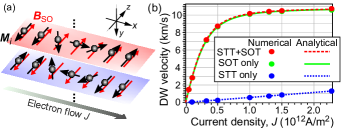
Figure 1: (a) Schematics of the system. (b) Numerical and analytical results of the DW velocities.

To explain this phenomenon, we analytically derive the formula of DW velocity [plotted with lines in Fig. 1(b)] by employing a simple two-layer model with presumed rigid DW profiles during the motion Parkin ; Mougin . The DW profiles are obtained from the saddle-point equation of the Hamiltonian as $\bm{M}_{l}=M(\sin\theta_{l}\cos\phi_{l},\sin\theta_{l}\sin\phi_{l},\cos\theta_{l})$ with $\theta_{\rm L}=-2\tan^{-1}[\exp\frac{x-q(t)}{\Delta}]$ and $\theta_{\rm U}=\theta_{\rm L}+\pi$, where $l$(=U, L) is an index of the upper and lower layers. Here $q(t)$ and $\Delta$ are the center coordinate and the width of the DW, respectively, and the tilt angle $\phi_{l}(t)$ is assumed to be spatially uniform Parkin ; Mougin . We plugged this formula into LLGS equation and confirmed that the DWs in the upper and lower layers have common $q(t)$ and $\Delta$ when the antiferromagnetic coupling $J_{\rm AF}$ is sufficiently strong.

After some algebra, we obtain a condtion for terminally static $\phi_{l}$ as $0=\dot{\phi}_{\rm U}(1+\alpha^{2})=u(\alpha-\beta)/\Delta-\gamma B_{\rm SO}-\alpha\gamma(J_{\rm AF}+K_{\rm h})\sin(2\phi_{\rm U})/M$, which leads to

$$\sin(2\phi_{\rm U}) = -\frac{M}{\alpha\gamma(J_{\rm AF}+K_{\rm h})}\Big{[}\frac{u(\beta-\alpha)}{\Delta}+\gamma B_{\rm SO}\Big{]},~{}$$ (2)

where $\phi_{\rm L}=-\phi_{\rm U}$. Note that this formula has the same form as that in a ferromagnetic thin film lying on the $xy$ plane Mougin , where $J_{\rm AF}+K_{\rm h}$ plays the same role as the demagnetization factor $N_{y}-N_{x}$ in the latter case. Therefore, we expect Walker breakdown also in the layered antiferromagnets Ruben2020 ; Mougin . Using Eq. (2), the DW velocity is derived as

$$v\equiv\dot{q} = u\frac{\beta}{\alpha}+\frac{\gamma B_{\rm SO}\Delta}{\alpha}.~{}$$ (3)

The right-hand side is a sum of two contributions from STT (the first term as in Thiaville ) and SOT (the second term). We, therefore, naively expect that the DW velocity $v$ in the presence of both STT and SOT is given by a simple sum as $v_{\rm both}=v_{\rm STT}+v_{\rm SOT}$ where $v_{\rm STT}$ ($v_{\rm SOT}$) is the velocity in the presence of STT (SOT) only. We also expect that $v$ is proportional to $u$ or the current density $j_{\rm e}$ because $B_{\rm SO}\propto u$. However, the normalized staggered magnetization $\bm{l}\equiv(\bm{M}_{\rm U}-\bm{M}_{\rm L})/2M$ in antiferromagnets follows the Lorentz-invariant equation of motion when the damping and the current-induced torques are compensated, and thus the DW width $\Delta$ suffers from a relativistic contraction Tatara01 ; WB_AF01 ; Shiino as $\Delta(v)\approx\Delta_{0}\sqrt{1-v^{2}/v^{2}_{g}}$, where $\Delta_{0}(=a_{0}\sqrt{J_{\rm F}/2K_{\rm e}})$ is the DW width in the static case and $v_{g}(=a_{0}\sqrt{J_{\rm F}J_{\rm AF}}/\hbar)$ is the magnon velocity in the exchange limit ($|\bm{m}|\equiv|(\bm{M}_{\rm U}+\bm{M}_{\rm L})/2M|\ll|\bm{l}|$, see SI Sec. X). Therefore, $v_{\rm both}$ should depend nonlinearly on the current density $u$ and the SO-field $B_{\rm SO}$, and the velocity is no longer given by a simple addition of $v_{\rm STT}+v_{\rm SOT}$.

With the formula of the Lorentz-contracted width $\Delta(v)$, Eq. (3) becomes a quadratic equation for $v$. One solution of this equation is negative and, thus, is unphysical because $\bm{j}_{\rm e}\propto+\hat{\bm{x}}$ gives rise to a net torque that should drive DW motion in the $+\hat{\bm{x}}$ direction (SI Sec. IX). The other solution is positive and thus is physical, which can be simplified as $v=u/(a\sqrt{c+du^{2}}-b)$ with constants $a=\gamma f_{\rm SO}/(FJ_{\rm AF})$, $b=2K_{\rm e}\alpha\beta/F$, $c=2J_{\rm AF}^{2}J_{\rm F}K_{\rm e}(a_{0}\alpha)^{2}$, $\ d=J_{\rm AF}\hbar^{2}F$, and $F=J_{\rm F}(\gamma f_{\rm SO}a_{0})^{2}-2K_{\rm e}\beta^{2}$. This simple analytical solution is the first major result of this study, which is shown by lines in Fig. 1(b) and coincides well with the numerical results. We show an alternative derivation based on the Thiele equation Thiele in SI Sec. VIII, which turns out to give the same formula for the DW velocity.

When $B_{\rm SO}=0$, $v$ is independent of $J_{\rm AF}$, which can be understood intuitively. A finite $B_{\rm SO}$ efficiently tilts $\bm{M}_{l}$ on both layers along the hard axis $-\hat{\bm{y}}$ direction (SI Sec. IX). Subsequently, the $J_{\rm AF}$ coupling induces a strong exchange torque owing to this tilt to drive DW motion Roy . This scenario is the same as that in the synthetic antiferromagnets Parkin , where the damping-like SOT is the dominant mechanism for the high DW speed. Note that Eq. (2) indicates that there is still a finite tilt angle even when $B_{\rm SO}=0$ owing to the STT. The DW velocity in this case is proportional to $(J_{\rm AF}+K_{\rm h})\Delta\sin(2\phi_{\rm U})$ (see SI Sec. II), and thus, the dependence on $J_{\rm AF}$ is cancelled, resulting in effectively uncoupled ferromagnetic DWs. In addition, in the limit of $u\rightarrow\infty$, we obtain $v\rightarrow v_{g}\sqrt{1-n}$, with $n=\frac{2K_{\rm e}}{J_{\rm F}}(\frac{\beta}{\gamma f_{\rm SO}a_{0}})^{2}\approx 4\times 10^{-4}$ using $\beta=10\alpha$. Therefore, we find that the DW velocity cannot exceed the magnon velocity $v_{g}$ as expected and can reach $v_{g}$ only in the adiabatic limit of $\beta=0$.

Magnon velocity and tilt angle.—We use a saddle-point solution of $\theta_{\rm U,L}$ to fit the simulated DW widths and evaluate $v_{g}$ numerically, which is close to the analytical value (SI Sec. IV). For $j_{\rm e}=1.5\times 10^{12}$ A/m², Eq. (2) leads to $\sin(2\phi_{\rm U})\approx-0.16$, and the DWs are within Walker regime to maintain the rigid moving profiles, which self-consistently justifies our initial substitution of the rigid DW profiles into the LLGS equation. This corresponds to $M_{\text{U/L},y}\approx-0.08M\text{sech}(\frac{x-vt}{\Delta(v)})$ with the same sign for both layers. This analytical result coincides well with the simulation results (SI Sec. IV). The minor discrepancy in the peak height is attributable to nonzero spin-wave emissions behind the moving DW indeed observed in the simulations.

Prediction of multiple Walker regimes.— The Walker breakdown is defined as a regime in which rigid DW profiles are no longer stable when driven by large current or strong field exceeding a threshold, with which $\dot{\phi}_{\rm U,L}$ becomes finite. In the breakdown regime, the right-hand side of Eq. (2) is greater than $1$ or less than $-1$, and thus the threshold current $u_{\rm c}$ is determined by the condition $\sin(2\phi_{\rm U}(u_{\rm c}))=\pm 1$. It has been widely believed that the Walker breakdown should not occur for DWs in antiferromagnets WB_AF01 ; WB_AF02 ; Shiino ; Baltz ; WB_AF03 . However, we find that it can occur in layered antiferromagnets with exchange coupling $J_{\rm AF}$ because Eqs. (2) and (3) have the same form as that for DWs in ferromagnetic thin films Mougin . Substituting the analytical solution of $v$ into Eq. (2), we obtain its $u$-dependence as $\sin(2\phi_{\rm U})=-c_{0}u\Big{[}1+\frac{(\beta-\alpha)(c_{1}+c_{2}u^{2})}{x_{1}\sqrt{1+c_{5}u^{2}}-x_{2}u^{2}}\Big{]}$ with coefficients specified in SI Sec. V. This indicates nonlinear $u$ dependence of $\sin(2\phi_{\rm U})$ and possible emergence of multiple Walker regimes separated by breakdown regimes with boundaries defined by $\sin(2\phi_{\rm U}(u_{\rm c}))=\pm 1$. This is in striking contrast to the case of ferromagnets, in which $\sin(2\phi)$ shows a monotonic behavior against $u$ and, thus, only a unique threshold current density appears Mougin ; Yang .

Figure 2 shows the current-density dependence of $\sin(2\phi_{\rm U})$ when $\beta=2\alpha$, in which we find multiple Walker regimes in (i) $0<u<u_{\rm c1}$ with $u_{\rm c1}\approx 10u_{0}$ and (ii) $u_{\rm c2}<u<u_{\rm c3}$ with $u_{\rm c2}\approx 178u_{0}$ and $u_{\rm c3}\approx 200u_{0}$, where $u_{0}\equiv(p\gamma\hbar a_{0}^{3}/2eM)\times 10^{12}$ A/m². There is also a singular point of $\sin(2\phi_{\rm U})$ at $u_{\rm s}=v_{g}\alpha/\beta\approx 93u_{0}$, at which the denominator vanishes as $x_{1}\sqrt{1+c_{5}u^{2}}-x_{2}u^{2}=0$. The equation for the threshold current, $\sin(2\phi_{\rm U}(u_{\rm c}))=\pm 1$, has no analytical solutions since it has a form $\sum^{6}_{n=1}\gamma_{n}u^{n}_{\rm c}=0$ with the sixth-order polynomial of $u_{\rm c}$ and coefficients $\gamma_{n}$. Nevertheless, it evidently implies that more than one Walker regimes can exist. This is another central result of this work. Note that the emergence of multiple Walker breakdowns can be expected also when $\beta<\alpha$ (see SI Sec. V), whereas only a single breakdown regime appears similar to the ferromagnetic case in the special condition of $\beta=\alpha$, which leads to $\sin(2\phi_{\rm U})=-c_{0}u$ and a unique threshold current density of $u_{\rm c}=1/c_{0}$.

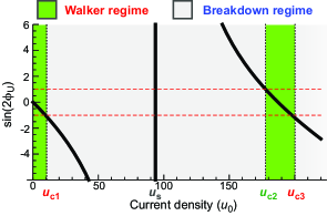
Figure 2: Thick solid (black) curves show $\sin(2\phi_{\rm U})$ when $\beta=2\alpha$. Horizontal dotted lines label the values $\pm 1$. Grey areas indicate the Walker breakdown regimes.

Averaged velocity in breakdown regimes.—In the Walker breakdown regimes, $\phi_{\rm U,L}(t)$ depends on time such that both $\sin(2\phi_{\rm U,L}(t))$ and $v(t)$ oscillate in time, and it is no longer permissible to use Eq. (2) to obtain Eq. (3). However, we can evaluate the time-averaged DW velocity $v_{\rm avg}$ by assuming that $\Delta(v(t))$ has reached a terminal value and it depends roughly on the averaged velocity as $\Delta(v(t))\approx\Delta(v_{\rm avg})$ via the Lorentz contraction. By solving the differential equation $\dot{\phi}_{\rm U}=A\sin(2\phi_{\rm U})+B$ with constants $A=\frac{-\alpha\gamma(J_{\rm AF}+K_{\rm h})}{M(1+\alpha^{2})}$ and $B=\frac{-u}{1+\alpha^{2}}(\frac{\beta-\alpha}{\Delta}+\gamma f_{\rm SO})$, we obtain the solution $\phi_{\rm U}(t)=\arctan[\frac{-A}{B}+\frac{\sqrt{B^{2}-A^{2}}}{B}\tan[\sqrt{B^{2}-A^{2}}(t+c)]]$ where $c$ is the integration constant. Real solutions require $B^{2}\geq A^{2}$, which leads to $u\geq u_{\rm th}=\frac{\alpha\gamma(J_{\rm AF}+K_{\rm h})\Delta(u_{\rm th})}{M[\gamma f_{\rm SO}\Delta(u_{\rm th})+(\beta-\alpha)]}$. This equation is exactly the same as that for $u_{\rm c1}$, i.e., $\sin(2\phi_{\rm U}(u_{\rm c1}))=-1$, and thus the relation $u_{\rm th}=u_{\rm c1}$ holds, which allows us to draw $v_{\rm avg}(u)$ in the first breakdown regime starting almost from $u_{\rm c1}$. By averaging over the period $\pi/\sqrt{B^{2}-A^{2}}$, we obtain $\langle\sin(2\phi_{U})\rangle=(-B-\sqrt{B^{2}-A^{2}})/A$ Yang .

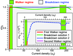
Figure 3: Theoretical DW velocities. Inset shows the enlarged graph. In the Walker (breakdown) regimes, the curves represent the terminal (time-averaged) velocity. Dotted curves are guides to the eyes.

Using this formula, we derive an equation for $v_{\rm avg}$, which is quartic in $v_{\rm avg}$ as $\sum^{4}_{n=0}d_{n}v^{n}_{\rm avg}=0$ (For concrete expressions of constants $d_{n}$, see SI Sec. VI). We solve this equation numerically and obtain four solutions. Two of them are negative or complex and thus unphysical (SI Sec. IX), whereas the other two are real and positive, which are plotted by solid (green) and dotted (blue) curves in Fig. 3. We find several significant differences from the case of DWs in ferromagnets Mougin ; Yang . First, the DW velocity in the Walker regimes given by Eq. (3) is not linear in $u$ because of the relativistic effect on the DW width, in contrast to the linear behavior in ferromagnets. Second, there are two solutions of $v_{\rm avg}$ in the breakdown regimes, one is smaller (solid green line) and the other is larger (dotted blue line) than the velocity before the breakdown (solid red line), in contrast to the unique velocity drop in ferromagnets Yang . Note that both solutions of $v_{\rm avg}$ are smaller than the magnon velocity $v_{g}$, indicating that the Lorentz invariance is still preserved in the breakdown regimes with high current density in our assumption of the contracted form of $\Delta(v_{\rm avg})$. Third, multiple Walker regimes appear, which is fundamentally distinct from the unique breakdown in ferromagnets.

In the presence of STT and staggered SOT, we can extend the consideration in Dasgupta ; Belashchenko ; Saarikoski to write the Lagrangian density for our layered antiferromagnet as,

$$\mathcal{L}=-\mathcal{J}\bm{m}\cdot[\bm{l}\times(\partial_{t}+u\partial_{x})\bm{l}]-4J_{\rm AF}\bm{m}^{2}/a_{0}-\mathcal{U}(\bm{l}),~{}$$ (4)

where $\mathcal{J}=M/\gamma a_{0}$ and $\mathcal{U}=J_{\rm F}a_{0}(\partial_{x}\bm{l})^{2}-K_{\rm e}l^{2}_{z}/a_{0}+K_{\rm h}l^{2}_{y}/a_{0}-(M/a_{0})\bm{l}\cdot\bm{B}_{\rm SO}$ is the energy density of $\bm{l}$. The $\mathcal{J}$ term is the spin Berry phase in a gauge with opposite Dirac strings $\bm{n}_{0,l}$ for the two sublattices in the monopole representation $\sum_{l}\mathcal{L}_{\text{B},l}=\frac{1}{\gamma a_{0}}\sum_{l}[\bm{n}_{0,l}\cdot\bm{M}_{l}\times(\partial_{t}+u\partial_{x})\bm{M}_{l}]/(1-\bm{n}_{0,l}\cdot\bm{M}_{l})$ and is expanded up to the second order of $\bm{m}$. (The next finite order of $\bm{m}$ is the third order which can be proved by choosing, e.g., $\bm{n}_{0}=\pm\hat{\bm{z}}$ for the two sublattices, respectively.) Dasgupta ; Belashchenko . The adiabatic STT contributes to the second term of the convective derivative $(\partial_{t}+u\partial_{x})$ Tatara2008 . Neglecting the nonadiabatic STT and Rayleigh dissipation ($\propto\alpha\dot{\bm{m}}^{2}$), we obtain $\bm{m}=-\mathcal{J}a_{0}\bm{l}\times(\partial_{t}+u\partial_{x})\bm{l}/(8J_{\rm AF})$ from the Lagrange equation. Using the saddle-point DW profile of $\bm{l}$, the $\bm{m}$-dependent terms after integrating over $x$ become $\frac{M_{0}}{2}(v-u)^{2}+\frac{I}{2}\dot{\phi}_{\rm U}^{2}$, which are the translational and rotational kinetic energies of a soliton with mass $M_{0}=M^{2}/(4\gamma^{2}a_{0}\Delta J_{\rm AF})$ and moment of inertia $I=M_{0}\Delta^{2}$. In this derivation, we assume a time-independent terminal $\Delta$.

Now we discuss which of the two positive solutions for $v_{\rm avg}$ is of more physical sense from this Lagrangian formalism. We note that near $u_{\rm c1}\approx 0.55$ km/s, the DW velocity $v$ is very close to the magnon velocity of $v_{g}\approx 10.77$ km/s, and thus $v(u_{\rm c1})$ is greater than $u_{\rm c1}$. When the system crosses the threshold $u_{\rm c1}$ and enters the breakdown regime, the soliton angular frequency $\dot{\phi}_{\rm U}$ changes abruptly from zero to finite, which causes a nonzero rotational energy. To preserve the kinetic energy of the soliton in a narrow current-density range near $u_{\rm c1}$, the DW velocity should decrease. Therefore, the solution 1 (solid green curve) in Fig. 3 can be a unique physical solution. From the experimental point of view, however, it should be mentioned that with extremely large current beyond $u_{\rm c1}$, several other instabilities and effects may appear such as spin-wave emissions Tatara_SWemit and DW proliferations Ruben2020 . Indeed, it was theoretically argued that an effective gyrofield induced by the kinetic energies of DW can cause the DW proliferation together with the transient Lorentz-invariance breaking with DW speeds exceeding $v_{g}$ Ruben2020 ; Guslienko .

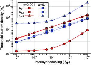
Figure 4: Threshold current density as functions of the interlayer antiferromagnetic coupling for weaker and stronger Gilbert damping, i.e., $\alpha$=0.001 and $\alpha$=0.1. The units of the vertical and horizontal axes are $u_{0}$ and $J_{\rm AF}$(=4.58$\times$10^-2 eV), respectively.

Proposal for experimental observations.—Since the values of $u_{\text{c}j}$ ($j=1,2,3$) in Fig. 2 are quite large ($u_{0}$ corresponds to $10^{12}$ A/m²), experimental feasibility and possible materials to observe our predictions should be argued. In synthetic antiferromagnets Parkin ; Parkin02 , an underlying Pt layer induces a damping-like SOT $\propto\bm{M}\times\bm{M}\times\hat{\bm{z}}$ (using our coordinate convention) in the same direction but with different strengths for the two magnetic layers on top of it (stacked along $-\hat{\bm{y}}$) Parkin . One can fabricate another Pt layer above the upper magnetic layer which, by symmetry, generates an opposite SOT when applying the current. In this situation, each layer is driven by opposite damping-like SOT. After taking a curl product of the LLGS equation with $\bm{M}$ to cancel time derivatives on its right-hand side, it induces a staggered field-like SOT $\propto\pm\bm{M}\times(\bm{M}\times\bm{M}\times\hat{\bm{z}})\propto\mp\bm{M}\times\hat{\bm{z}}$, which mimics the staggered SO-field $\bm{B}_{\rm SO}$ in our case. Therefore, we expect similar results of multiple Walker breakdowns to occur in synthetic antiferromagnets with both top and bottom Pt layers.

Because the interlayer coupling $J_{\rm AF}$ can be tuned in synthetic antiferromagnets by changing the thickness of metallic layer sandwiched by two magnetic layers, we investigate the dependence of $u_{\text{c}j}$ on $J_{\rm AF}$ as well as the Gilbert damping $\alpha$ when $\beta=2\alpha$ with other parameters following that of Mn₂Au. The results plotted in Fig. 4 show monotonic decrease of $u_{\text{c}j}$ as $J_{\rm AF}$ decreases, with $u_{\rm c2}$ down to an experimentally feasible value of $\sim 10^{12}$ A/m² when $J_{\rm AF}$ is as small as $\approx 4.58\times 10^{-6}$ eV. Moreover, the results indicate that for a larger damping of $\alpha=0.1$, the upper Walker regime between $u_{\rm c2}$ and $u_{\rm c3}$ appears in a wider range, which is appropriate for experimental observations.

Conclusion.—We have theoretically studied the DW motion in layered antiferromagnets driven by electric current, which exerts both STT and staggered SOT. We have discovered possible reentrant emergence of multiple Walker breakdowns, which is in sharp contrast to the unique Walker breakdown for the current-driven DW motion in ferromagnets. We have revealed that the Lorentz contraction of DW width in antiferromagnets gives rise to nonlinear current-dependence of the DW velocity and the predicted multiple Walker breakdowns. The dominant efficiency of SOT over STT and their non-additive effects in driving the DW motion have been also demonstrated. It should be mentioned that the present theory can be generalized in the straightforward way for intrinsic antiferromagnetic systems in which STT is not applicable or for the cases in which other torques due to additional effects are present (e.g., Dzyaloshinskii-Moriya interaction, Rashba spin-orbit interaction, spin Hall effect). Our findings are expected to be observed in synthetic antiferromagnets experimentally and provide siginificant contributions to development of the antiferromagnetic spintronics.

This work is supported by Japan Society for the Promotion of Science KAKENHI (Grant No. 20H00337 and No. 23H04522), CREST, the Japan Science and Technology Agency (Grant No. JPMJCR20T1) , and the Waseda University Grant for Special Research Project (Project No. 2023C-140). M.K.L. is grateful for illuminating discussions with Rintaro Eto, Collins A. Akosa, and Xichao Zhang.

References

- (1) T. Jungwirth, X. Marti, P. Wadley, and J. Wunderlich, Nat. Nanotech. 11, 231 (2016).
- (2) E. V. Gomonay and V. M. Loktev, Low Temp. Phys. 40, 17 (2014).
- (3) P. Wadley, B. Howells, J. Zlezný, C. Andrews, V. Hills, R. P. Campion, V. Novák, K. Olejník, F. Maccherozzi, S. S. Dhesi, S. Y. Martin, T. Wagner, J. Wunderlich, F. Freimuth, Y. Mokrousov, J. Kuneš, J. S. Chauhan, M. J. Grzybowski, A. W. Rushforth, K. W. Edmonds, B. L. Gallagher, T. Jungwirth, Science 351, 587 (2016).
- (4) J. Železný, H. Gao, K. Výborný, J. Zemen, J. Mašek, A. Manchon, J. Wunderlich, J. Sinova, and T. Jungwirth, Phys. Rev. Lett. 113, 157201 (2014).
- (5) S. H. Yang, K. S. Ryu, and S. Parkin, Nat. Nanotech. 10, 221 (2015).
- (6) R. A. Duine, K.-J. Lee, S. S. P. Parkin, and M. D. Stiles, Nat. Phys. 14, 217 (2018).
- (7) T. Moriyama, W. Zhou, T. Seki, K. Takanashi, and T. Ono, Phys. Rev. Lett. 121 167202 (2018).
- (8) T. Dohi, S. DuttaGupta, S. Fukami, and H. Ohno, Nat. Comm. 10 5153 (2019).
- (9) C. A. Akosa, O. A. Tretiakov, G. Tatara, A. Manchon, Phys. Rev. Lett. 121 097204 (2018).
- (10) X. Zhang, Y. Zhou, and M. Ezawa, Sci. Rep. 6, 24795 (2016).
- (11) A. Salimath, Fengjun Zhuo, R. Tomasello, G. Finocchio, and A. Manchon, Phys. Rev. B 101, 024429 (2020).
- (12) L. Shen, J. Xia, X. Zhang, M. Ezawa, O. A. Tretiakov, X. Liu, G. Zhao, and Y. Zhou, Phys. Rev. Lett. 124, 037202 (2020).
- (13) A. Mougin, M. Cormier, J. P. Adam, P. J. Metaxas, and J. Ferré, Europhys. Lett. 78, 57007 (2007).
- (14) J. Yang, C. Nistor, G. S. D. Beach, and J. L. Erskine, Phys. Rev. B 77, 014413 (2008).
- (15) O. Gomonay, T. Jungwirth, and J. Sinova, Phys. Rev. Lett. 117, 017202 (2016).
- (16) S. Selzer, U. Atxitia, U. Ritzmann, D. Hinzke, and U. Nowak, Phys. Rev. Lett. 117, 107201 (2016).
- (17) T. Shiino, S.-H. Oh, P. M. Haney, S.-W. Lee, G. Go, B.-G. Park, and K.-J. Lee, Phys. Rev. Lett. 117, 087203 (2016).
- (18) V. Baltz, A. Manchon, M. Tsoi, T. Moriyama, T. Ono, and Y. Tserkovnyak, Rev. Mod. Phys. 90, 015005 (2018).
- (19) O. Gomonay, T. Jungwirth, and J. Sinova, physica status solidi (RRL), Rapid Research Letters 11, 1700022 (2017).
- (20) R. M. Otxoa, P. E. Roy, R. Rama-Eiroa, J. Godinho, K. Y. Guslienko, and J. Wunderlich, Commun. Phys. 3, 190 (2020).
- (21) P. E. Roy, R. M. Otxoa, and J. Wunderlich, Phys. Rev. B 94, 014439 (2016).
- (22) N. B. Weber, H. Ohldag, H. Gomonaj, and F. U. Hillebrecht, Phys. Rev. Lett. 91, 237205 (2003).
- (23) T. Kampfrath, A. Sell, G. Klatt, A. Pashkin, S. M’́ahrlein, T. Dekorsy, M. Wolf, M. Fiebig, A. Leitenstorfer, and R. Huber, Nat. Photonics 5, 31 (2011).
- (24) L. D. Landau and E. M. Lifshitz, Phys. Z. Sowjetunion 8 153 (1935).
- (25) T. L. Gilbert, Phys. Rev. 100 1243 (1955).
- (26) S. Zhang and Z. Li, Phys. Rev. Lett. 93 127204 (2004).
- (27) G. Tatara and H. Kohno, Phys. Rev. Lett. 92 086601 (2004).
- (28) A. Thiaville, Y. Nakatani, J. Miltat, and Y. Suzuki, Europhys. Lett. 69, 990 (2005).
- (29) G. Tatara, C. A. Akosa, and R. M. Otxoa de Zuazola, Phys. Rev. Research 2, 043226 (2020).
- (30) A. A. Thiele, Phys. Rev. Lett. 30, 230 (1973).
- (31) S. Dasgupta, S. K. Kim, and O. Tchernyshyov, Physical Review B 95, 220407 (2017).
- (32) K. D. Belashchenko, O. Tchernyshyov, A. A. Kovalev, and O. A. Tretiakov, Applied Physics Letters 108, 132403 (2016).
- (33) H. Saarikoski, H. Kohno, C. H. Marrows, G. Tatara, Phys. Rev. B 90, 094411 (2014).
- (34) G. Tatara, H. Kohno, J. Shibata, Phys. Rep. 468, 213 (2008).
- (35) G. Tatara and R. M. Otxoa de Zuazola, Phys. Rev. B 101, 224425 (2020).
- (36) K. Y. Guslienko, K. S. Lee, and S. K. Kim, Phys. Rev. Lett. 100, 027203 (2008).