Fast Algorithms for Finite Element nonlinear Discrete Systems to Solve the PNP Equations

Abstract The Poisson-Nernst-Planck (PNP) equations are one of the most effective model for describing electrostatic interactions and diffusion processes in ion solution systems, and have been widely used in the numerical simulations of biological ion channels, semiconductor devices, and nanopore systems. Due to the characteristics of strong coupling, convection dominance, nonlinearity and multiscale, the classic Gummel iteration for the nonlinear discrete system of PNP equations converges slowly or even diverges. We focus on fast algorithms of nonlinear discrete system for the general PNP equations, which have better adaptability, friendliness and efficiency than the Gummel iteration. First, a geometric full approximation storage (FAS) algorithm is proposed to improve the slow convergence speed of the Gummel iteration. Second, an algebraic FAS algorithm is designed, which does not require multi-level geometric information and is more suitable for practical computation compared with the geometric one. Finally, improved algorithms based on the acceleration technique and adaptive method are proposed to solve the problems of excessive coarse grid iterations and insufficient adaptability to the size of computational domain in the algebraic FAS algorithm. The numerical experiments are shown for the geometric, algebraic FAS and improved algorithms respectively to illustrate the effiency of the algorithms.

Keywords: Poisson-Nernst-Planck equations, Gummel iteration, full approximation storage; adaptive and acceleration technology

AMS(2000)subject classifications 65N30, 65N55

1 Introduction

The Poisson-Nernst-Planck (PNP) equations are a coupled nonlinear partial differential equations, which describe electrostatic interactions and diffusion processes in ion solution systems. They were first proposed by Nernst ^[1] and Planck^[2] and have been widely used in the numerical simulations of biological ion channel^{[3, 4, 5]}, semiconductor devices^{[6, 7, 8]}, and nanopore systems^{[9, 10].} Due to the strong coupling, convection dominance, nonlinearity, and multiscale characteristics of PNP practical problems, it is difficult to construct numerical methods with good approximation, stability and efficiency. Many numerical methods have been applied to solve the PNP equations, such as finite element (FE) ^{[11, 12, 13, 14]}, finite difference ^{[15, 16, 17, 18]}, and finite volume ^{[19, 20, 21, 22]} methods, etc. Since there exist problems such as the poor stability or the bad approximation when using standard FE, finite difference or finite volume methods to discretize pratical PNP equations, some improved methods have emerged. The inverse average FE method was constructed for a class of steady-state PNP equations in nanopore systems in [23], which effectively solves the problems of non physical pseudo oscillations caused by convection dominance. A new stable FE method called SUPG-IP was proposed in [24] for the steady-state PNP equations in biological ion channel. Numerical experiments showed that the method has better performance than the standard FE and SUPG methods in positive conservation and robustness. The robustness and stability of the FE algorithm in channel numerical simulation were improved in [25] for the modified PNP equations considering ion size effects by using the SUPG method and pseudo residual free bubble function technique. In [26], the Slotboom variable was used to transform the continuity equation into an equivalent equation for a class of steady-state PNP equations in semiconductor, and then four FE methods with averaging techniques were introduced to discretize the nonlinear system. Numerical experiments have shown that the new methods can ensure the conservation of the calculated terminal current and are as stable as the SUPG method.

The above nonlinear discrete systems are usually linearized by iterative methods such as Gummel or Newton, and then fast algorithms are designed for these linear systems. In [27], the Newton linearization was used for the adaptive finite volume discrete system of PNP equation on unstructured grid, and algebraic multigrid (AMG) method was applied to solve the linearized system. In [28], a fast FGMRES algorithm was designed based on a block upper triangular preconditioner for the edge average finite element (EAFE) scheme of the Newton linearized PDEs of the PNP and Navier-Stokes coupled system, in which the PNP subsystem was solved using the PGMRES based on the UA-AMG preconditioner. Xie and Lu ^[12] used Slotboom transformation to transform the PNP equations with periodic boundary conditions into equivalent equations, and gave an acceleration method for the Gummel iteration, in which the nonlinear potential equation was solved by the modified Newton iterative method. Since the discrete system of the practical PNP problem has the characteristics of strong asymmetry, coupling between physical quantities, multi-scale, large scale and condition number, the above iterative algorithms may have slow convergence (even divergence) and low computational efficiency. There is another kind of method at present, whose basic idea is based on the two-grid method ^[29], which essentially transforms the nonlinear discrete system on the fine grid to the nonlinear system on the coarse grid. Shen et. al. ^[30] proposed a two-grid FE method for a class of time-dependent PNP equations. Based on the optimal $L^{2}$ norm error estimates of the derived discrete scheme, the $H^{1}$ norm error estimates are presented. Comparative experiments with Gummel iteration show that the new method has higher computational efficiency. Ying et. al. ^[13] aimed at the two-grid FE method of the SUPG scheme for the steady-state PNP equations in biological ion channel, in which the Krylov iterative method based on the block Gauss-Seidel preconditioner was designed for the Newton linearized system on the coarse grid, and it was proved that the condition number of the preconditioned system is independent of the mesh size under certain assumptions. It should be pointed out that although the above geometric two-grid method has higher computational efficiency than Gummel or Newton iterative method for some discrete systems of PNP equations, it may encounter many difficulties when the method is applied to solve complex practical PNP problems. For example, the approximate accuracy depends on the coarsening rate. Due to factors such as low smoothness of the solution, the coarsening rate cannot be too large, which affects the acceleration effect. In addition, complex meshes generated by professional/commercial softwares are usually difficult to meet the requirements of geometric two-grid method for nested meshes. Therefore, further research is needed on fast algorithms for PNP large-scale discrete systems. The FAS algorithm proposed by Brandt ^[31] is a nonlinear geometric multigrid method. It has been applied to direct solutions of many nonlinear systems ^{[32, 33, 34, 35]}, the detailed descriptions of which refer to e.g. [36, 37, 38]. The FAS algorithm requires multi-level grid information, and at present coarse grids are mainly generated through aggregation methods ^{[39, 40]}. However, for complex domains and unstructured grids, aggregation algorithms lead to poor quality of coarse grids, which in turn affects the performance of the FAS algorithm ^[39]. Therefore, it is important to study the algebraic FAS algorithm directly from the discretized nonlinear algebraic system of the PNP equations. In addition, due to the drawbacks of existing linearized methods for solving PNP discrete systems, such as insufficient adaptability to the size of domain and excessive iterations for solving corresponding nonlinear algebraic systems on coarse grid ^{[41, 23]}, further improvements on them will be worthwhile.

In this paper, we mainly study the fast algorithms of the finite element nonlinear discrete system to solve the PNP equations. First, for nonlinear discrete systems of general PNP equations, in order to overcome the drawbacks of slow convergence speed and weak adaptability to size of computational domain in the classical Gummel iteration, a geometric FAS algorithm is designed. Compared with the Gummel iteration, it not only has higher efficiency but also enhances the adaptability to convective intensity. Second, considering the limitations of the geometric FAS algorithm, such as the requirement of nested coarse grids, an algebraic FAS algorithm is presented. This algorithm does not require multi-level geometric information, which is more suitable for practical PNP problems. The numerical experiments including a practical problem in ion channel show that the algebraic FAS algorithm can not only improve the efficiency of decoupling external iterations, but also expand the domain of the problem that can be solved compared with the Gummel iteration, which indicates the effectiveness of this algorithm in solving the strong coupling and convection dominated PNP equations. Finally, some improved algorithms based on acceleration technique and adaptive method are designed to deal with the problems of excessive coarse grid iterations and insufficient adaptability to the size of computational domain in the algebraic FAS algorithm when the convective intensity is high. Numerical experiments show that the improved algorithms converge faster and significantly enhances the adaptability of convective intensity. The rest of paper is organized as follows. In Section 2, we introduce some standard notations and PNP equations. The continuous and discrete forms are also given in this section. In Section 3, we show the geometric and algebraic FAS algorithms. The improved algrithms based on the acceleration technique and adaptive method are also presented in this section. The conclusion is presented in Section 4.

2 The continuous and discrete problems

Let $\Omega\subset\mathbb{R}^{d}$ $(d=2,3)$ be a bounded Lipschitz domain. We clarify the standard notations for Sobolev spaces $W^{s,p}(\Omega)$ and their associated norms and seminorms. For $p=2$, we denote $H^{s}(\Omega)=W^{s,2}(\Omega)$ and $H_{0}^{1}(\Omega)=\{v\in H^{1}(\Omega):v|_{\partial\Omega}=0\}$. For simplicity, let $\|\cdot\|_{s}=\|\cdot\|_{W^{s,2}(\Omega)}$ and $\|\cdot\|=\|\cdot\|_{L^{2}(\Omega)}$ and $(\cdot,\cdot)$ denote the standard $L^{2}$-inner product.

2.1 PNP equations

We consider the following time-dependent PNP equations (cf. [30])

$$\left\{\begin{array}[]{lr}-\Delta\phi-\sum\limits^{2}_{i=1}q^{i}p^{i}=f,&\text{ in }\Omega,~{}\text{for}~{}t\in(0,T],\vspace{1mm}\\ {\partial_{t}p^{i}}-\nabla\cdot(\nabla{p^{i}}+q^{i}p^{i}\nabla\phi)=F^{i},&\text{ in }\Omega,~{}\text{for}~{}t\in(0,T],i=1,2,\vspace{1mm}\end{array}\right.$$ (2.1)

where $p^{i},~{}i=1,2$ is the concentration of the $i$-th ionic species with charge $q^{i}$, $p_{t}^{i}=\frac{\partial p^{i}}{\partial t}$, $\phi$ denotes the electrostatic potential, $f$ and $F^{i}$ are the reaction source terms, The homogeneous Dirichlet boundary conditions are employed

$$\left\{\begin{array}[]{c}\;\phi=0,\;\text{on}\;\partial\Omega,~{}\text{for}~{}t\in(0,T],\vspace{0.5mm}\\ \;p^{i}=0,\;\text{on}\;\partial\Omega,~{}\text{for}~{}t\in(0,T].\end{array}\right.$$ (2.2)

The corresponding steady-state PNP equations are as follows (cf. [42])

$$\left\{\begin{array}[]{lr}-\Delta\phi-\sum\limits^{2}_{i=1}q^{i}p^{i}=f,&\text{ in }\Omega,~{}\text{for}~{}t\in(0,T],\vspace{1mm}\\ -\nabla\cdot(\nabla{p^{i}}+q^{i}p^{i}\nabla\phi)=F^{i},&\text{ in }\Omega,~{}\text{for}~{}t\in(0,T],i=1,2,\vspace{1mm}\end{array}\right.$$ (2.3)

The weak formulations of (2.1)-(2.2) and (2.3)-(2.2) are that: find $p^{i}\in L^{2}(0,T;H_{0}^{1}(\Omega))$ $\cap L^{\infty}(0,T;L^{\infty}(\Omega))$, $i=1,2$, and $\phi(t)\in H_{0}^{1}(\Omega)$ such that

$$(\nabla\phi,\nabla w)-\sum\limits^{2}_{i=1}q^{i}(p^{i},w)=(f,w),~{}~{}\forall w\in H_{0}^{1}(\Omega),$$ (2.4)

$$(\partial_{t}p^{i},v)+(\nabla{p^{i}},\nabla v)+(q^{i}p^{i}\nabla\phi,\nabla v)=(F^{i},v),~{}~{}\forall v\in H_{0}^{1}(\Omega),~{}i=1,2.$$ (2.5)

and find $p^{i}\in H_{0}^{1}(\Omega),~{}i=1,2$ and $\phi\in H_{0}^{1}(\Omega)$ such that

$$(\nabla\phi,\nabla w)-\sum\limits^{2}_{i=1}q^{i}(p^{i},w)=(f,w),~{}~{}\forall w\in H_{0}^{1}(\Omega),$$ (2.6)

$$(\nabla{p^{i}},\nabla v)+(q^{i}p^{i}\nabla\phi,\nabla v)=(F^{i},v),~{}~{}\forall v\in H_{0}^{1}(\Omega),~{}i=1,2,$$ (2.7)

respectively.

The existence and uniqueness of the solutious to (2.4)-(2.5) and (2.6)-(2.7) have been presented in [43] for $F^{i}=r(p^{1},p^{2})(1-p^{1}p^{2})$. Here $p^{1},~{}p^{2}$ represent the densities of mobile holes and electrons respectively in a semiconductor device. The function $r:R_{+}^{2}\rightarrow R_{+}$ are required to be Lipschitzian and $p^{1},~{}p^{2}\in W^{0,\infty}(\Omega)$.

2.2 The discrete scheme

Suppose $\mathcal{T}_{h}=\{K\}$ is a partition of $\Omega$, where $K$ is the element and $h=\max\limits_{K\in\mathcal{T}_{h}}\{\mbox{diam}~{}K\}$. We define the first order finite element subspace of $H_{0}^{1}(\Omega)$ as follows

$$V_{h}=\{v\in H^{1}(\Omega):v|_{\partial\Omega}=0~{}\mbox{and}~{}v|_{K}\in\mathcal{P}_{1}(K),~{}~{}\forall K\in\mathcal{T}_{h}\},$$ (2.8)

where $\mathcal{P}_{1}(K)$ is the set of linear polynomials on the element $K$.

The semi-discretization to (2.4)-(2.5) is defined as follows: find $p^{i}_{h},~{}i=1,2$ and $\phi_{h}\in V_{h}$ such that

$$(\nabla\phi_{h},\nabla w_{h})-\sum\limits^{2}_{i=1}q^{i}(p^{i}_{h},w_{h})=(f,w_{h}),~{}~{}\forall w_{h}\in V_{h},$$ (2.9)

$$(\partial_{t}p^{i}_{h},v_{h})+(\nabla{p^{i}_{h}},\nabla v_{h})+(q^{i}p^{i}_{h}\nabla\phi_{h},\nabla v_{h})=(F^{i},v_{h}),~{}~{}\forall v_{h}\in V_{h},~{}i=1,2.$$ (2.10)

In order to present the full discrete approximation to (2.1)-(2.2), let $0=t^{0}<t^{1}<\cdots<t^{N}=T$ denote the partition of $[0,T]$ into subintervals $(t^{n-1},t^{n})$ such that $\tau=\max\{t^{n}-t^{n-1},n=1,2,\cdots N\}$. For any function $u$, denote by

$$u^{n}(x)=u(x,t^{n})$$

and

$$D_{\tau}u^{n+1}=\frac{u^{n+1}-u^{n}}{\tau},~{}\mbox{for}~{}n=0,1,2,\cdots,N-1.$$

The backward Euler full discretization based on FE method for (2.1)-(2.2) is: Find $p_{h}^{i,n+1}\in V_{h},~{}i=1,2$ and $\phi_{h}^{n+1}\in V_{h}$, such that

$$(\nabla\phi_{h}^{n+1},\nabla w_{h})-\sum\limits_{i=1}^{2}q^{i}(p_{h}^{i,n+1},w_{h}) =(f^{n+1},w_{h}),\forall w_{h}\in V_{h},$$ (2.11)

$$(D_{\tau}p_{h}^{i,n+1},v_{h})+(\nabla p_{h}^{i,n+1},\nabla v_{h})+(q^{i}p_{h}^{i,n+1}\nabla\phi^{n+1}_{h},\nabla v_{h}) =(F^{i,n+1},v_{h}),\forall v_{h}\in V_{h},$$ (2.12)

where $f^{n+1}=f(t^{n+1},\cdot)$, $F^{i,n+1}=F^{i}(t^{n+1},\cdot),~{}i=1,2$.

There exist some convection dominated PNP equations in semiconductor area, for which the standard FE method does not work well. The EAFE method has shown advantages in solving convection dominated equations. In order to present the EAFE scheme for PNP equations, suppose $K$ denotes the element with the number $k$, and $E$ is the edge with the endpoints $x_{k_{\nu}}$ and $x_{k_{\mu}}$, where ${k_{\nu}}$ is the whole number corresponding to the local number $\nu$. Let $\tau_{E}=x_{k_{\nu}}-x_{k_{\mu}},~{}{k_{\nu}}<{k_{\mu}}$ for any $E$ in $\mathcal{T}_{h}$.

The EAFE fully discrete scheme for PNP equations is: find $p^{i,n+1}_{h}\in V_{h},~{}i=1,2$ and $\phi_{h}^{n+1}\in V_{h}$, satisfying

$$(\nabla\phi_{h}^{n+1},\nabla w_{h}) -\sum\limits_{i=1}^{2}q^{i}(p_{h}^{i,n+1},w_{h})=(f^{n+1},w_{h}),~{}\forall w_{h}\in V_{h},$$ (2.13)

$$(D_{\tau}p_{h}^{i,n+1},v_{h}) +\sum\limits_{K\in\mathcal{T}_{h}}[\sum\limits_{E\subset K}\omega_{E}^{K}\tilde{\alpha}^{K,i}_{E}(\phi_{h}^{n+1})\delta_{E}(e^{q^{i}\phi_{h}^{n+1}}p_{h}^{i,n+1})\delta_{E}v_{h}]=\sum\limits_{K\in\mathcal{T}_{h}}(F^{i,n+1},v_{h})_{K},~{}\forall v_{h}\in V_{h},$$ (2.14)

where

$$\tilde{\alpha}^{K,i}_{E}(\phi_{h}^{i,n+1})=\left(\frac{1}{|\tau_{E}|}\int_{E}e^{q^{i}\phi^{n+1}_{h}}\mathrm{d}s\right)^{-1},~{}\omega_{E}^{K}:=\omega_{E_{\nu\mu}}^{K}=-(\nabla\psi_{k_{\mu}},\nabla\psi_{k_{\nu}})_{K},~{}\delta_{E}(u)=u_{k_{\nu}}-u_{k_{\mu}},~{}u=e^{q^{i}\phi_{h}}p_{h}^{i}.$$ (2.15)

To present the corresponding discrete algebraic system, we define some notations. Let

$$\Psi=(\psi_{1},\ldots,\psi_{{n_{h}}}),~{}{n_{h}}=\dim(V_{h})$$ (2.16)

be a set of basis function vectors of $V_{h}$. Note that $\forall v_{h}\in V_{h}$, we have

$$v_{h}|_{K}=\sum_{m=1}^{4}V_{k_{m}}\lambda^{K}_{m}=\lambda^{K}V_{K},$$ (2.17)

where $\lambda^{K}=(\lambda^{K}_{1},\lambda^{K}_{2},\lambda^{K}_{3},\lambda^{K}_{4})$ and $V_{K}=(V_{k_{1}},V_{k_{2}},V_{k_{3}},V_{k_{4}})^{T}$ are the volume coordinate vector and degree of freedom vector of element K, respectively. Assume $n_{h}$ dimensional vectors

$$\Phi^{n+1}=(\Phi^{n+1}_{1},\ldots,\Phi^{n+1}_{n_{h}})^{T},\quad G_{\Phi}^{n+1}=((f^{n+1},\psi_{1}),\ldots,(f^{n+1},\psi_{n_{h}}))^{T},$$ (2.18)

and $2n_{h}$ dimensional vectors

$$P^{\mu}=\begin{pmatrix}P^{1,\mu}\\ P^{2,\mu}\end{pmatrix},~{}~{}P^{i,\mu}=(p^{i,\mu}_{1},\ldots,p^{i,\mu}_{n_{h}})^{T},~{}\mu=n,n+1,~{}i=1,2,$$ (2.19)

$$G^{n+1}=\begin{pmatrix}G^{1,n+1}\\ G^{2,n+1}\end{pmatrix},~{}G^{i,n+1}=(g^{i,n+1}_{1},\ldots,g^{i,n+1}_{n_{h}})=((F^{i,n+1},\psi_{1}),\ldots,(F^{i,n+1},\psi_{n_{h}}))^{T},~{}i=1,2,$$ (2.20)

$n_{h}\times 2n_{h}$ lumped mass matrix

$$\bar{M}=-(q^{1}M,q^{2}M),~{}M=\frac{1}{4}\textrm{diag}(|\Omega_{1}|,\cdots,|\Omega_{n_{h}}|),~{}\Omega_{k}=supp(\psi_{k}),~{}k=1,\ldots,{n_{h}},$$ (2.21)

and $n_{h}\times n_{h}$ stiffness matrix

$$A_{L}=(\nabla\Psi^{T},\nabla\Psi).$$ (2.22)

It is easy to know the nonlinear algebraic equation for the EAFE discrete system  (2.13)-(2.14) is as follows:

$$A_{1}(U_{1})U_{1}=F_{1}.$$ (2.23)

Here

$$A_{1}(U_{1}):=\left(\begin{array}[]{cc}A_{1}^{\Phi}&\bar{M}_{1}\\ \bf 0&A_{1}^{P}(\Phi_{1})\\ \end{array}\right),~{}U_{1}=\left(\begin{array}[]{c}\Phi_{1}\\ P_{1}\end{array}\right),~{}F_{1}=\left(\begin{array}[]{c}F_{1}^{\Phi}\\ F_{1}^{P}\end{array}\right),$$ (2.24)

where

$$A_{1}^{\Phi}=A_{L},~{}\bar{M}_{1}=\begin{pmatrix}-q^{1}M_{1}&-q^{2}M_{1}\end{pmatrix},~{}M_{1}=M,~{}A_{1}^{P}(\Phi_{1}):={\bf M}+\tau\bar{A}(\Phi^{n+1}),$$ (2.25)

$$\Phi_{1}=\Phi^{n+1},~{}P_{1}=P^{n+1},~{}F^{\Phi}=G_{\Phi}^{n+1},~{}F^{P}=F^{n}.$$ (2.26)

matrix ${\bf M}=diag(M,M)$, $\bar{M}$ and $A_{L}$ are defined by (2.21) and (2.22), respectively, $2n_{h}\times 2n_{h}$ stiffness matrix

$$\bar{A}(\Phi^{n+1})=diag(\bar{A}^{1}(\Phi^{n+1}),\bar{A}^{2}(\Phi^{n+1})),$$ (2.27)

the general element of the element stiffness matrix  $\bar{A}^{i,K}(\Phi^{n+1})$ on tetrahedron element $K$ for $\bar{A}^{i}(\Phi^{n+1})$ is as follows:

$$\bar{a}_{\nu\mu}^{i,K}(\Phi^{n+1})=\left\{\begin{array}[]{ll}&-\omega^{K}_{E_{\nu\mu}}\tilde{\alpha}_{E_{\nu\mu}}^{K,i}(\Phi^{n+1})e^{q^{i}\lambda^{K}(q_{\mu})\Phi^{n+1}_{K}},{\nu>\mu},\\ &-\omega^{K}_{E_{\mu\nu}}\tilde{\alpha}_{E_{\mu\nu}}^{K,i}(\Phi^{n+1})e^{q^{i}\lambda^{K}(q_{\mu})\Phi^{n+1}_{K}},{\nu<\mu},\\ &\sum\limits_{k>\mu}\omega^{K}_{E_{\mu k}}\tilde{\alpha}_{E_{\mu k}}^{K,i}(\Phi^{n+1})e^{q^{i}\lambda^{K}(q_{\mu})\Phi^{n+1}_{K}}\\ &+\sum\limits_{k<\mu}\omega^{K}_{E_{k\mu}}\tilde{\alpha}_{E_{k\nu_{2}}}^{K,i}(\Phi^{n+1})e^{q^{i}\lambda^{K}(q_{\mu})\Phi^{n+1}_{K}},{\nu=k},\end{array}\right.~{}\nu,\mu=1,2,3,4,~{}i=1,2,$$ (2.28)

where $\omega^{K}_{E_{\nu\mu}}$ is defined by (2.15), $q_{1},q_{2},q_{3},q_{4}$ are four vertices of element $K$, and

$$\tilde{\alpha}^{K,i}_{E_{\nu\mu}}(\Phi^{n+1})=\left[\frac{1}{|\tau_{E}|}\int_{E}e^{q^{i}\lambda^{K}\Phi^{n+1}_{K}}\mathrm{d}s\right]^{-1}.$$ (2.29)

3 Fast algorithms for PNP equations

In this section, first a geometric FAS algorithm is proposed, which can overcome the slow convergence speed of the classical Gummel algorithm for the nonlinear discrete systems of general PNP equations. Then due to the limitation of the geometric FAS algorithm, such as the requirement for nested coarse grids, an algebraic FAS algorithm is designed. However, the algebraic FAS algorithm still has drawbacks such as too many coarse grid iterations when encountering the problem of strong convection dominance. Hence, we design some improved algorithms based on the acceleration technique and adaptive method.

3.1 Geometric and algebraic FAS algorithms

In this subsection, we first present the geometric FAS algorithm, then design algebraic FAS algorithm. Numerical examples show the FAS algorithm improves the efficiency of the decoupling iterations and expands the computational domain of PNP equations.

3.1.1 Geometric FAS algorithm

The geometric FAS algorithm for PNP equations is as shown in Algorithm 3.1, which can be constructed by following [31, 44] and using the Gummel iteration for PNP equations ^[42].

Algorithm 3.1 Geometric FAS Algorithm

Setup:

S1.

Generate two nested grids $\mathcal{T}_{h_{l}},~{}l=1,2,~{}h_{1}<h_{2}$. Let $V_{h_{l}}$ be the corresponding linear FE function space, $n_{l}=\dim(V_{h_{l}})$; Take prolongation operator $P_{2}^{1}$ as the linear FE interpolantion function from $V_{h_{2}}$ to $V_{h_{1}}$.

S2.

Generate restriction operator $R_{1}^{2,u}:V_{h_{1}}\rightarrow V_{h_{2}}$. The general element of the corresponding matrix $R_{1}^{2,u}\in R^{n_{2}\times n_{1}}$ is defined by

$$R_{1}^{2,u}(i,j)=\left\{\begin{array}[]{ll}\frac{R_{1}^{2}(i,j)}{\sum\limits_{j=1}^{n_{1}}R_{1}^{2}(i,j)},&\hbox{$R_{1}^{2}(i,j)\neq 0$;}\\ 0,&\hbox{else,}\end{array}\right.,$$ (3.1)

where $R_{1}^{2}=(P_{2}^{1})^{T}$ (see Remark 3.1 for the reason why two sets of restriction operators are needed.)

S3.

Obtain the submatrix $A^{\Phi}_{l}$ and $\bar{M}_{l}$ of the stiffness matrix $A_{l}(\cdot)$ corresponding to (2.13)-(2.14) on grids $\mathcal{T}_{h_{l}},l=1,2$, and load vector $F_{l}$, and give the intial value $U_{1}^{(0)}$, the stopping tolerance $\epsilon$ and $\epsilon_{c}$, and the maximum number $M_{iter}$ of iterations on the coarse and fine grids.

Solve:

For any $l\geq 0$, The FAS iteration from $U_{1}^{(l)}\rightarrow U_{1}^{(l+1)}$ is as follows.

S1.

Pre-smoothing: Take $U_{1}^{(l)}$ as the initial value, and then perform $\nu_{1}\geq 0$ iterations by using Gummel iteration.

S2.

Solving coarse grid system: Solve the following nonlinear system on the coarse grid using Gummel iteration

$$A_{2}\left(U_{2}\right)U_{2}=\tilde{\tau}_{2}.$$ (3.2)

Here

$$\tilde{\tau}_{2}:=A_{2}\left(y_{2}\right)y_{2}+\vec{R}_{1}^{2}r_{1},~{}y_{2}=\vec{R}_{1}^{2,u}U_{1}^{(fs)},~{}r_{1}=F_{1}-A_{1}\left(U_{1}^{(fs)}\right)U_{1}^{(fs)},$$ (3.3)

where

$$\vec{R}_{1}^{2}=diag(R_{1}^{2},R_{1}^{2},R_{1}^{2}),~{}\vec{R}_{1}^{2,u}=diag(R_{1}^{2,u},R_{1}^{2,u},R_{1}^{2,u}).$$ (3.4)

S3.

Correction:

$$U_{1}^{(bs)}=U_{1}^{(fs)}+(\vec{R}_{1}^{2})^{T}(U_{2}-y_{2}).$$ (3.5)

S4.

Post-smoothing: Choosing $U_{1}^{(bs)}$ as the initial value, perform $\nu_{2}\geq 0$ iterations for (2.23) by using Gummel iteration and get $U_{1}^{(l+1)}$.

Remark 3.1.

The matrix $R_{1}^{2,u}$ is the transfer matrix between degrees of freedom from $V_{h_{1}}$ to $V_{h_{2}}$. The matrix $R_{1}^{2}$ is the transfer matrix between the basis funcitons from $V_{h_{1}}$ to $V_{h_{2}}$. Since the row sum of $R_{1}^{2}$ may not be $1$, e.g. it may not satisfies the constant approximation, it can not be the trasfer operator between degrees of freedom and it needs to generate $R_{1}^{2,u}$ to transfer degrees of freedom which satisfies constant approximation.

For given tolerance $\epsilon$, the exit criterion for Algorithm 3.1 is $l+1\geq$ $M_{iter}$ or

$$\|F_{1}-A_{1}(U_{1}^{(l+1)})U_{1}^{(l+1)}\|_{R^{3n_{1}}}\leq\epsilon.$$ (3.6)

If take $U_{1}^{(0)}=\bf 0$, $\nu_{1}=0$ in the geometric FAS algorthm (Algorithm 3.1), then from $r_{1}=F_{1}=((f_{3},\Psi_{1}),(f_{1},\Psi_{1}),(f_{2},\Psi_{1}))^{T}$ and $\Psi_{2}=R_{1}^{2}\Psi_{1}$, where $\Psi_{i},~{}i=1,2$ is the FE basis function vector on grid $\mathcal{T}_{h_{i}}$, we have

$$\tilde{\tau}_{2}=\vec{R}_{1}^{2}r_{1}=((f_{3},R_{1}^{2}\Psi_{1}),(f_{1},R_{1}^{2}\Psi_{1}),(f_{2},R_{1}^{2}\Psi_{1}))^{T}=((f_{3},\Psi_{2}),(f_{1},\Psi_{2}),(f_{2},\Psi_{2}))^{T}=F_{2},$$

where $F_{2}$ is right hand of the coarse grid equation in the two-grid (TG) algorithm provided in [30, 13]. Hence, the TG algorithm can be viewed as a degradation of Algorithm 3.1 in the case when $U_{1}^{(0)}=\bf 0$, $\nu_{1}=0$, $\nu_{2}=1$.

Next we present a numerical example to observe the efficiency of geometric FAS algorithm and compare it with the Gummer iteration [14] and TG algorithm [30, 13]. First, we study the approximation effect of the Gummel iteration and TG algorithm under different convection intensity. Then we present the results of the geometric FAS algorithm and compare it with the Gummel and TG algorithms.

Example 3.1.

Consider the following steady-state PNP equations

$$\left\{\begin{array}[]{llll}&-\Delta u-(p-n)=f,&&\text{ in }\Omega,\\ &-\nabla\cdot\left(\nabla p+c_{\lambda}p\nabla u\right)=F^{p},&&\text{ in }\Omega,\\ &-\nabla\cdot\left(\nabla n-c_{\lambda}n\nabla u\right)=F^{n},&&\text{ in }\Omega,\end{array}\right.$$ (3.7)

with boundary conditions

$$\left\{\begin{array}[]{l}u=g_{u},\text{on}\;\partial\Omega,\vspace{0.5mm}\\ p=g_{p},\;\text{on}\;\partial\Omega,~{}i=1,2,\\ n=g_{n},\;\text{on}\;\partial\Omega,~{}i=1,2.\end{array}\right.$$ (3.8)

Here $\Omega=[-0.5,0.5]^{3}$, $c_{\lambda}=0.179L^{2}=1.79$, the right hand function and the boundary value are given by the following exact solution

$$\left\{\begin{array}[]{ll}u=\cos(\pi x)\cos(\pi y)\cos(\pi z),&\\ p=3\pi^{2}(1+\frac{1}{2}\cos(\pi x)\cos(\pi y)\cos(\pi z)),&\\ n=3\pi^{2}(1-\frac{1}{2}\cos(\pi x)\cos(\pi y)\cos(\pi z)).&\end{array}\right.$$ (3.9)

The meshes used are uniform tetrahedral meshes, the tolerance $\epsilon=1E-6$, the maximum iteration number $M_{iter}$=1000, linear systems are solved by the direct method solver Pardiso. For similicity, denote by $e_{\zeta}=u_{h}-u$ and $\zeta=u,p,n$.

Due to the fact that $c_{\lambda}=0.179L^{2}$ in (3.7) represents the convection coefficient, we show the errors of the Gummel iteration (see Tables 1-3) and the number of iteration (see Table 4) with different $L$ to observe the impact of convection intensity on the Gummel iteration. It is shown on Tables 1-3 show the $L^{2}$ and $H^{1}$ norm errors with different $L$, which indicates that the Gummel iteration is effective to solve PNP equations on uniform tetrahedral meshes when $L$ is not large. Howevever, if $L$ gets larger, which means strong convection dominance appears, the Gummel iterations converges very slowly even diverges, see Table 4.

Table 1: Error of Gummel iteration when $h=\frac{1}{8}$

$L$	$\|e_{u}\|_{0}$	$\|e_{p}\|_{0}$	$\|e_{n}\|_{0}$	$\|e_{u}\|_{1}$	$\|e_{p}\|_{1}$	$\|e_{n}\|_{1}$
$1$	2.32E-02	4.00E-01	4.06E-01	4.80E-01	7.10	7.10
$\sqrt{2.6}$	2.43E-02	4.08E-01	4.32E-01	4.80E-01	7.11	7.11
$\sqrt{2.7}$	2.43E-02	4.08E-01	4.33E-01	4.80E-01	7.11	7.11

Table 2: Error of Gummel iteration when $h=\frac{1}{16}$

$L$	$\|e_{u}\|_{0}$	$\|e_{p}\|_{0}$	$\|e_{n}\|_{0}$	$\|e_{u}\|_{1}$	$\|e_{p}\|_{1}$	$\|e_{n}\|_{1}$
$1$	6.04E-03	1.03E-01	1.05E-01	2.43E-01	3.60	3.60
$\sqrt{2.6}$	6.12E-03	1.08E-01	1.14E-01	2.43E-01	3.60	3.60
$\sqrt{2.7}$	6.36E-03	1.04E-01	1.11E-01	2.43E-01	3.60	3.60

Table 3: Error of Gummel iteration when $h=\frac{1}{32}$

$L$	$\|e_{u}\|_{0}$	$\|e_{p}\|_{0}$	$\|e_{n}\|_{0}$	$\|e_{u}\|_{1}$	$\|e_{p}\|_{1}$	$\|e_{n}\|_{1}$
$1$	2.16E-03	2.25E-02	2.34E-02	1.22E-01	1.80	1.80
$\sqrt{2.6}$	2.46E-03	1.65E-02	1.72E-02	1.22E-01	1.80	1.80
$\sqrt{2.7}$	8.65E-04	3.98E-02	4.16E-02	1.22E-01	1.81	1.81

Table 4: The number of iterations of Gummel iteration

	1	$\sqrt{2.6}$	$\sqrt{2.7}$	$\sqrt{2.8}$
$\frac{1}{8}$	11	175	557	*
$\frac{1}{16}$	9	118	273	*
$\frac{1}{32}$	7	85	188	*

where $*$ means the algorithm diverges.

Next, we compare the result of Gummel iteration with that of TG algorithm. Tables 5-6 display the results of the two algorithms on uniform tetrahedral meshes, where the coarsening rates are 1:8 and 1:64 respectively when the sizes of the coarse and fine grid are $\frac{1}{16}(\frac{1}{8})$ and $\frac{1}{16}(\frac{1}{4})$, respectively.

Table 5: Errors for Gummel and TG algorithms with $L=1$

$h(H)$	$\|e_{u}\|_{0}$	$\|e_{p}\|_{0}$	$\|e_{n}\|_{0}$	$\|e_{u}\|_{1}$	$\|e_{p}\|_{1}$	$\|e_{n}\|_{1}$
Gummel-$\frac{1}{16}$	1.03E-02	7.49E-02	8.03E-02	2.44E-01	3.60	3.60
TG-$\frac{1}{16}(\frac{1}{8})$	2.34E-02	4.59E-02	4.47E-02	2.63E-01	3.64	3.62
TG-$\frac{1}{16}(\frac{1}{4})$	1.16E-02	2.97E-01	2.16E-01	4.43E-01	4.18	3.97

Table 6: Errors for Gummel and TG algorithms with $L=\sqrt{2.7}$

$h(H)$	$\|e_{u}\|_{0}$	$\|e_{p}\|_{0}$	$\|e_{n}\|_{0}$	$\|e_{u}\|_{1}$	$\|e_{p}\|_{1}$	$\|e_{n}\|_{1}$
Gummel-$\frac{1}{16}$	9.09E-03	5.47E-02	7.49E-02	2.43E-01	3.61	3.60
TG-$\frac{1}{16}(\frac{1}{8})$	1.79E-02	9.67E-02	8.40E-02	2.52E-01	3.73	3.71
TG-$\frac{1}{16}(\frac{1}{4})$	5.34E-02	6.13E-01	5.69E-01	3.67E-01	5.40	5.20

It is seen from Tables 5-6 that the $H^{1}$ and $L^{2}$ norm errors of the two algorithms are similar when the size $L$ of the computational domain is small. However, the errors of the TG algorithm is larger than that of the Gummul algorithm when $L$ is larger. For example, the errors $\|e_{p}\|_{0}$ of the TG algorithm with coarsening rates 1:8 and 1:64 are about 2 and 10 times that of the Gummel algorithm, respectively when $L=\sqrt{2.7}$.

Next, we investigate the adaptability of the geometric FAS algorithm to the size $L$. Tables 7-8 show the number of iterations and errors of algorithm 3.1 on uniform tetrahedral meshes with a coarsening rate of 1:8, i.e., a mesh size of $\frac{1}{16}(\frac{1}{8})$ . In the computation, the number of pre-smoothing and post-smoothing times is $\nu_{1}=\nu_{2}=1$, stop tolerances $\epsilon=1E-6$ and $\epsilon_{c}=1E-7$, iter and iter-c respectively represent the number of iterations and the average number of coarse grid iterations of the geometric FAS algorithm.

Table 7: Errors of geometric FAS algorithm when $h(H)=\frac{1}{16}(\frac{1}{8})$

$L$	iter(iter-c)	$\|e_{u}\|_{0}$	$\|e_{p}\|_{0}$	$\|e_{n}\|_{0}$	$\|e_{u}\|_{1}$	$\|e_{p}\|_{1}$	$\|e_{n}\|_{1}$
${1}$	3(7)	1.03E-02	7.49E-02	8.03E-02	2.44E-01	3.60	3.60
$\sqrt{1.5}$	3(10)	9.80E-03	6.96E-02	7.56E-02	2.44E-01	3.60	3.60
$\sqrt{2.7}$	5(24)	9.19E-03	6.08E-02	6.58E-02	2.43E-01	3.60	3.60
$\sqrt{2.8}$	5(27)	9.14E-03	6.05E-02	6.54E-02	2.43E-01	3.60	3.60
$\sqrt{2.9}$	5(27)	9.14E-03	6.05E-02	6.54E-02	2.43E-01	3.60	3.60
$\sqrt{3.0}$	5(34)	9.02E-03	6.01E-02	6.47E-02	2.43E-01	3.60	3.60
$\sqrt{3.8}$	7(426)	8.79E-03	5.72E-02	6.01E-02	2.43E-01	3.60	3.60

Table 8: Errors of geometric FAS algorithm when $h(H)=\frac{1}{32}(\frac{1}{16})$

$L$	iter(iter-c)	$\|e_{u}\|_{0}$	$\|e_{p}\|_{0}$	$\|e_{n}\|_{0}$	$\|e_{u}\|_{1}$	$\|e_{p}\|_{1}$	$\|e_{n}\|_{1}$
${1}$	2(7)	2.46E-03	1.96E-02	2.09E-02	1.22E-01	1.80	1.80
$\sqrt{1.5}$	2(11)	2.05E-03	2.05E-02	2.20E-02	1.22E-01	1.80	1.80
$\sqrt{2.7}$	3(42)	2.18E-03	1.68E-02	1.84E-02	1.22E-01	1.80	1.80
$\sqrt{2.8}$	3(53)	2.14E-03	1.70E-02	1.87E-02	1.22E-01	1.80	1.80
$\sqrt{3.1}$	3(183)	2.04E-03	1.77E-02	1.98E-02	1.22E-01	1.80	1.80

Combining the two tables above with Tables 4, 2, 3 and 6, we can see

(1)

Compared with the Gummel algorithm, the geometric FAS algorithm can calculate larger size of computational domain. For example, the Gummel algorithm does not converge such as when $h=\frac{1}{16}$, $L=\sqrt{2.8}$, but the geometric FAS algorithm can be applied to the cases with larger $L$, such as $L=\sqrt{3.8}$. When the size $L$ is the same, the FAS algorithm can achieve the same accuracy as the Gummel algorithm and converge faster than it, such as the number of iterations of the Gummel algorithm is about 18 times that of the FAS algorithm when $h=\frac{1}{16}$, $L=\sqrt{2.7}$.

(2)

Compared with the TG algorithm, the geometric FAS algorithm has higher accuracy when $L$ is larger. In addition, since TG needs to call linearized methods such as the Gummel algorithm on the coarse grid level, it can be seen from (1) that the geometric FAS algorithm can calculate a larger computational size than the TG algorithm. For example, the approximate upper limit of the size that the TG algorithm can calculate is about $L=\sqrt{2.7}$ when $h=\frac{1}{32}$, while that is more than $L=\sqrt{3.1}$ for the FAS algorithm.

Due to the fact that the geometric FAS algorithm usually requires users to provide geometric information of multiple layers of grids and nested grids, it is difficult to apply the geometric FAS algorithm to complex problems. Designing a reasonable algebraic FAS algorithm is an effective way to make up this defect. At present, there have been some preliminary research works in this area, e.g. a coarse grid construction method based on element aggregations is provided in [39, 40] . Next an effective algebraic FAS algorithm is presented for the PNP equation (2.23).

3.1.2 Algebraic FAS algorithm

In this subsection, we first introduce some notations used in the abgebraic FAS algorithm, then present the algebraic FAS algorithm and apply it to solve PNP equations including a practical problem in ion channel.

For any real matrix $A=(a_{ij})_{n\times n}$, denote by

• The dependency set of node $i$

  $$N_{i}=\{j\neq i~{}|~{}a_{ij}\neq 0\}.$$

• The influence set of node $i$

  $$N_{i}^{T}=\{j~{}|~{}i\in N_{j}\}.$$

• For the given strong and weak threshold $\theta_{1}$ and row sum parameter $\theta_{2}$, the strong dependency set $S_{i}$ of node $i$ is defined as follows:

  • If $\theta_{2}=1$, or $\theta_{2}\in(0,1)$ and $\bigg{|}\frac{\sum\limits_{j=1}^{n}a_{ij}}{a_{ii}}\bigg{|}\leq\theta_{2}$, then

    $$S_{i}=\{j\in N_{i}~{}\big{|}~{}a_{ij}\left\{\begin{array}[]{l}\geq\theta_{1}\max\limits_{k\neq i}\{a_{ik}\},~{}~{}a_{ii}<0\\ \leq\theta_{1}\min\limits_{k\neq i}\{a_{ik}\},~{}~{}a_{ii}\geq 0\end{array}\right.\}.$$

  • If $\theta_{2}\in(0,1)$ and  $\bigg{|}\frac{\sum\limits_{j=1}^{n}a_{ij}}{a_{ii}}\bigg{|}>\theta_{2}$, then $S_{i}=\emptyset.$

• Condition C1 of C/F splitting ^[45]:

  • Setting $i\in F$, $\exists~{}k\in C$, such that $k\in S_{i}$;

  • Setting $i,j\in F$, and if $j\in S_{i}$, then $\exists~{}k\in S_{i}\cap C$, such that $k\in S_{j}$.

• C/F splitting satisfies condition C2: $C$ is a certain maximal independent set of $V$, that is, there is no strong dependency or influence relationship between any two elements in $C$.

Next, the algebraic type FAS algorithm is presented by combining the coarsening algorithm, interpolation matrix generation algorithm, and geometric FAS algorithm of AMG method.

Algorithm 3.2 Algebraic type FAS algorithm

Setup:

S1.

Generate single level grid $\mathcal{T}_{h_{1}}$ and submatrix  $A^{\Phi}_{1}$ of stiffness matrix  $A_{1}(\cdot)$ corresponding to the discrete system  (2.13)-(2.14) on $\mathcal{T}_{h_{1}}$, $\bar{M}_{1}$ and right hand vector $F_{1}$.

S2.

Get the transfer operator between coarse and fine level.

S2.1

Generate CF array by Algorithm 3.3, denote the number of $C$ points by $n_{2}^{a}$, and interpolation matrix  $P_{1}^{2,a}$ from coase level to fine level.

S2.2

Get degrees of freedom transfer matrix $R_{1}^{2,u,a}\in R^{n_{2}^{a}\times n_{1}}$, the general element of which is defined by

$$R_{1}^{2,u,a}(i,j)=\left\{\begin{array}[]{ll}\frac{R_{1}^{2,a}(i,j)}{\sum\limits_{j=1}^{n_{1}}R_{1}^{2,a}(i,j)},&\hbox{if $R_{1}^{2,a}(i,j)\neq 0$;}\\ 0,&\hbox{else,}\end{array}\right.,$$ (3.11)

where $R_{1}^{2,a}=(P_{2}^{1,a})^{T}$.

S3.

Generate the following submatrix of the coarse grid operator $A_{2}(\cdot)$

$$A^{\Phi}_{2}=R_{1}^{2,a}A^{\Phi}_{1}P_{2}^{1,a},~{}M_{2}=R_{1}^{2,a}M_{1}P_{2}^{1,a},$$ (3.12)

and give the initial value  $U_{1}^{(0)}$, stopping tolerance $\epsilon$ and $\epsilon_{c}$ between coarse and fine level, and maximum times $M_{iter}$ of iteration .

Solve:

For any $l\geq 0$, the algorithm procedure from  $U_{1}^{(l)}\rightarrow U_{1}^{(l+1)}$ is as follows:

S1.

Pre-smoothing: Given initial value $U_{1}^{(l)}$, perform $\nu_{1}\geq 0$ times Gummel iteration to get $U_{1}^{(fs)}$.

S2.

Soving the following nonlinear system on the coarse grid by Algorithm 3.4

$$A_{2}\left(U_{2}\right)U_{2}=\tilde{\tau}_{2}.$$ (3.13)

Here

$$A_{2}(\cdot)=\vec{R}_{1}^{2,a}A_{1}((\vec{R}_{1}^{2,a})^{T}(\cdot))(\vec{R}_{1}^{2,a})^{T},~{}\tilde{\tau}_{2}:=\vec{R}_{1}^{2,a}A_{1}((\vec{R}_{1}^{2,a})^{T}y_{2})y_{2}+\vec{R}_{1}^{2,a}r_{1},$$ (3.14)

where $r_{1}$ is given by (3.3),

$$\vec{R}_{1}^{2,a}=diag(R_{1}^{2,a},R_{1}^{2,a},R_{1}^{2,a}),~{}y_{2}=\vec{R}_{1}^{2,u,a}U_{1}^{(fs)},~{}\vec{R}_{1}^{2,u,a}=diag(R_{1}^{2,u,a},R_{1}^{2,u,a},R_{1}^{2,u,a}).$$ (3.15)

S3.

Correction on coarse grid:

$$U_{1}^{(bs)}=U_{h_{1}}^{(fs)}+(\vec{R}_{1}^{2,a})^{T}(U_{2}-y_{2}).$$ (3.16)

S4.

Post-smoothing : Taking $U_{1}^{(bs)}$ as the initial value, perform $\nu_{2}\geq 0$ times Gummel iteration to get $U_{1}^{(l+1)}$.

Algorithms  3.3 and  3.4 used above are descripted as follows.

Algorithm 3.3 Generate CFmarker array and interpolate matrix $P_{1}^{2,a}$

S1

Given coarsing times $k$, strong and weak threshold $\theta_{1}$, row sum parameter $\theta_{2}$, the finest grid matrix $A_{1}$, generate array CF_marker_l on each level and interpolant matrix $P_{l}$ between coarse and fine level. For $l=1,\ldots,k$, perform

S1.1

Get strong connectivity matrix $S_{l}\in R^{n_{l}\times n_{l}}$, the general element of which is

$$S_{l}(i,j)=\left\{\begin{array}[]{l}1,~{}~{}j\in S_{i}^{l};\\ 0,~{}~{}otherwise.\end{array}\right.$$

S1.2

Let the set of numbers of the degrees of freedoms on level $l$ be $V_{l}=\{1,2,\cdots,n_{l}\}$. Perform C/F splitting for $V_{l}$ by using $S_{l}$, and get the C/F property array ^[45],

$$\text{ CF\_marker\_l}(i)=\begin{cases}-1,&\mbox{if}~{}i\in F_{l}\\ 1,&\mbox{if}~{}i\in C_{l}\end{cases},~{}C_{l}\cup F_{l}=V_{l},~{}C_{l}\cap F_{l}=\emptyset,$$

which strictly satisfies C1 condition, and tries to satisfy C2 condition ^[45].

S1.3

Get interpolant matrix $P_{l}\in R^{n_{l}\times n_{l+1}}$ from the grid $(l+1)$ to grid $l$, the general element pf which satisfies

$$P_{l}(i,j)=-\frac{1}{a^{l}_{ii}+\sum\limits_{k\in D_{i}^{w,l}\cup F^{l}_{i}}a^{l}_{ik}}\left(a^{l}_{ij}+\sum\limits_{k\in D_{i}^{s,l}\backslash F^{l}_{i}}\frac{a^{l}_{ik}\hat{a}^{l}_{kj}}{\sum\limits_{m\in C^{l}_{i}}\hat{a}^{l}_{km}}\right),$$

where

$$\hat{a}^{l}_{ij}=\left\{\begin{array}[]{ll}0,&\text{if sign}(a^{l}_{ij})=\text{sign}(a^{l}_{ii}),\\ a^{l}_{ij},&\text{otherwise}.\end{array}\right.$$

S1.4

Generate the coefficient matrix on grid $(l+1)$

$$A_{l+1}=P_{l}^{T}A_{l}P_{l}=(a_{ij}^{l+1})_{n_{l+1}\times n_{l+1}}.$$ (3.17)

S2

Merge layer by layer for  CF_marker_l to get two-level CFmarker needed and corresponding $n_{2}^{a}\times n_{1}$ prolongation matrix $P_{1}^{2,a}=\Pi_{l=1}^{k}P_{l}$, where $n_{2}^{a}=n_{k+1}$.

Algorithm 3.4 Gummel algorithm on coarse system (3.13)

Setup:

Generate matrix $A_{2}^{\Phi}$, $\bar{M}_{2}$ and $\tilde{\tau}_{2}$ from (3.12) and (3.14), and give the initial value $U_{2}^{(0)}$, stopping tolerance $\epsilon_{c}$ and maximum number $M_{iter}$ of iterations.

Solve:

For $l\geq 0$, Gummel iteration from $U_{2}^{(l)}\rightarrow U_{2}^{(l+1)}$ is as follow

S1.

Solve the following linear system

$$A_{2}^{\Phi}\Phi_{2}^{(l+1)}=\tilde{\tau}_{2}^{\Phi}-\bar{M}_{2}P_{2}^{(l)};$$ (3.18)

S2.

Generate $A_{2}^{P}(\Phi_{2}^{(l+1)})=R_{1}^{2,a}A_{1}^{P}(P_{2}^{1,a}\Phi_{2}^{(l+1)})P_{2}^{1,a}.$

S3.

Solve the linear system

$$A_{2}^{P}(\Phi_{2}^{(l+1)})P_{2}^{(l+1)}=\tilde{\tau}_{2}^{P};$$ (3.19)

S4.

If

$$\|\tilde{\tau}_{2}-A_{2}(U_{2}^{(l+1)})U_{2}^{(l+1)}\|_{R^{3n_{2}^{a}}}\leq\epsilon_{c},$$ (3.20)

or $l+1\geq M_{iter}$, then set $U_{1}=U_{1}^{(l+1)}$. Otherwise let $l\leftarrow l+1$, return  S1 and continue.

Next, we compare the geometric FAS algorithm, a coarsening rate which is 1:8, with the algebraic FAS algorithm on two non-uniform grids.

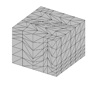
Figure 1: $\mathcal{T}_{h}^{1}$: Diagram of Kershaw grid with s=0.3

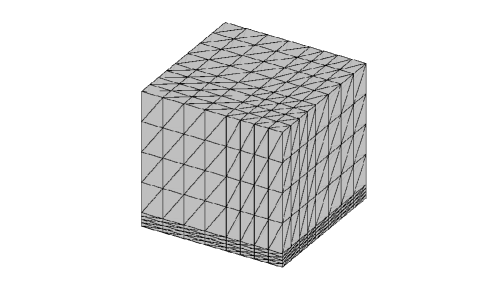
Figure 2: $\mathcal{T}_{h}^{2}$: Diagram of perturbation Kershaw grid with s=0.2

Figure 2 shows the Kershaw grid ^[46], where $s=(0,0.5]$ represents the degree of mesh distortion (The worse the quality of mesh becomes as the smaller $s$ is. It is a uniform mesh when $s=0.5$). Figure 2 shows a perturbation grid, which is obtained from a uniform grid by perturbing internal nodes as follows

$$x=\left\{\begin{array}[]{ll}a+(b-a)(1-s)(i-1)/nx,&\hbox{$2\leq i\leq\frac{nx}{2}+1$ ;}\\ \tilde{a}_{2}+(b-\tilde{a}_{2})\frac{i-\frac{nx}{2}+1}{nx/2},&\hbox{$\frac{nx}{2}+1<i\leq nx$ ;}\end{array}\right.$$

$$y=\left\{\begin{array}[]{ll}a+(b-a)(1-s)(j-1)/ny,&\hbox{$2\leq j\leq\frac{ny}{2}+1$ ;}\\ \tilde{a}_{2}+(b-\tilde{a}_{2})\frac{j-\frac{ny}{2}+1}{ny/2},&\hbox{$\frac{ny}{2}+1<j\leq ny$ ;}\end{array}\right.$$

$$z=\left\{\begin{array}[]{ll}a+(b-a)s(k-1)/nz,&\hbox{$2\leq k\leq\frac{nz}{2}+1$ ;}\\ \tilde{a}_{1}+(b-\tilde{a}_{1})\frac{k-\frac{nz}{2}+1}{nz/2},&\hbox{$\frac{nz}{2}+1<k\leq nz$ ;}\end{array}\right.$$

where $\tilde{a}_{1}=a+\frac{(b-a)s}{2}$, $\tilde{a}_{2}=a+\frac{(b-a)(1-s)}{2}$, the left and right endpoints $a=-0.5,~{}b=0.5$ of the interval, $nx=ny=nz$ are the numbers of partitions in the $x$, $y$, $z$ directions, respectively.

The following two tables display the number of iterations and errors of the corresponding discrete system of the geometric FAS and algebraic FAS algorithms for Example 3.1 on two sets of grids $\mathcal{T}_{h}^{1}$ and $\mathcal{T}_{h}^{2}$, where $s$ represents the degree of perturbation of grid, iter and iter-c are the iteration times of FAS and the average iteration times of coarse grid, respectively.

Table 9: Errors on $\mathcal{T}_{h}^{1}$ with $h=\frac{1}{12}$ and $L=\sqrt{3.5}$

	s	iter(iter-c)	$\|e_{u}\|_{0}$	$\|e_{p}\|_{0}$	$\|e_{n}\|_{0}$	$\|e_{u}\|_{1}$	$\|e_{p}\|_{1}$	$\|e_{n}\|_{1}$
geometric FAS	0.4	13(30)	2.10E-02	1.20E-01	1.66E-01	3.77E-01	5.60	5.57
algebraic FAS	0.4	7(41)	2.10E-02	1.20E-01	1.66E-01	3.77E-01	5.60	5.57
geometric FAS	0.3	12(30)	5.10E-02	3.04E-01	3.97E-01	5.98E-01	8.94	8.82
algebraic FAS	0.3	7(19)	5.10E-02	3.04E-01	3.97E-01	5.98E-01	8.94	8.82

Table 10: Errors on $\mathcal{T}_{h}^{2}$ with $h=\frac{1}{16}$ and $L=\sqrt{3.0}$

	s	iter(iter-c)	$\|e_{u}\|_{0}$	$\|e_{p}\|_{0}$	$\|e_{n}\|_{0}$	$\|e_{u}\|_{1}$	$\|e_{p}\|_{1}$	$\|e_{n}\|_{1}$
geometric FAS	0.3	8(31)	1.41E-02	9.58E-02	1.02E-01	3.01E-01	4.46	4.46
algebraic FAS	0.3	7(22)	1.41E-02	9.58E-02	1.02E-01	3.01E-01	4.46	4.46
geometric FAS	0.2	14(29)	1.47E-02	9.87E-02	1.05E-01	3.10E-01	4.59	4.59
algebraic FAS	0.2	6(27)	1.47E-02	9.88E-02	1.05E-01	3.10E-01	4.59	4.59

From the above two tables, it can be seen that the geomeric FAS algorithm needs more iterations than algebraic one when $L$ is large, the errors of both under the same $h$ are almost the same, and there are too many iterations on coarse grid for both of them. For instance, the number of iterations of the geometric FAS algorithm with $s=0.4$ is about twice that of the algebraic one, and numbers of the iteration on the coarse grid of both algorithms are greater than or equal to 30.

Next we present an example of practical PNP equations in ion channel. Since the mesh used in ion channel is unstructured grid, it is difficult to get natrual coarse grid. Hence the geometric FAS algorithm is not suitable and we use algebraic FAS algorithm 3.2 to solve the practical PNP problem and compare the result with that of Gummel iteration from the error, convergence speed and CPU time.

Example 3.2.

Consider the following PNP equations for simulating Gramicidin A(gA) ion channel in 1:1 CsCl solution with valence $+1$ and $-1$ ^[41]:

$$\left\{\begin{array}[]{ll}-\nabla\cdot\Big{(}-D_{i}\left(\nabla p^{i}+\frac{e}{K_{B}T}q^{i}p^{i}\nabla\phi\right)\Big{)}=0,\text{in}~{}\Omega_{s},~{}i=1,2,\\ -\nabla\cdot(\epsilon\nabla\phi)=\lambda\sum\limits_{i=1}^{2}q^{i}p^{i}+\rho^{f},~{}\text{ in}~{}\Omega=\Omega_{s}\cup\bar{\Omega}_{m},\end{array}\right.$$ (3.21)

where the unknown function $\phi$ is electrostatic potential and $p^{1}$ and $p^{2}$ are the concentrations of positive and negative ion, respectively. Here $\Omega=[-15,15]\times[-15,15]\times[-30,30]{\AA}$, $\Omega_{s}$ represents the bulk regions, $\Omega_{m}$ represents the membrane and protein region, the diffusion coefficient  $D_{1}=2.0561\times 10^{-9}\mathrm{~{}m}^{2}/\mathrm{s}$, $D_{2}=2.0321\times 10^{-9}\mathrm{~{}m}^{2}/\mathrm{s}$, charges $q^{1}=1$ and $q^{2}=-1$, elementary charge $e=1.6\times 10^{-19}\mathrm{C}$, Boltzmann constant $K_{B}=4.14\times 10^{-21}\mathrm{J}$, the dielectric coefficient $\epsilon(x)=\left\{\begin{array}[]{ll}2\epsilon_{0}\ ,~{}\mbox{in}~{}\Omega_{m}\\ 80\epsilon_{0},~{}\mbox{in}~{}\Omega_{s}\end{array}\right.$, with permittivity of vacuum $\varepsilon_{0}=8.85\times 10^{-12}\mathrm{C}^{2}/\left(\mathrm{N}\mathrm{m}^{2}\right)$, $\lambda=\left\{\begin{array}[]{ll}0,~{}\mbox{in}~{}\Omega_{m}\\ 1,~{}\mbox{in}~{}\Omega_{s}\end{array}\right.$, $\rho^{f}({\bf x})=\sum\limits_{j}^{N_{m}}q_{j}\delta({\bf x}-{\bf x_{j}})$ is an ensemble of singular atomic charges $q_{j}$ located at $x_{j}$ inside the protein.

Let $\Gamma=\partial\Omega_{s}\cap\partial\Omega_{m}$ be the interface that intersect the membrane and the bulk region, see the red curve in Figure 3, $\partial\Omega_{1}$ is the part of boundary of $\Omega$ that perpendicular to $z$ axis (suppose the channel is along the $z$ axis), $\partial\Omega_{2}$ is the part of boundary of $\Omega$ that is along the channel, $\partial\Omega_{3}=\partial\Omega\setminus\Gamma$ is the surface of the bulk region from which the interface of membrane $\Gamma$ is removed.

The interface and boundary conditions are

$$[\phi]=0,~{}[\epsilon\frac{\partial\phi}{\partial\upsilon^{m}}]=0,~{}~{}\mbox{on}~{}~{}\Gamma$$ (3.22)

and

$$\left\{\begin{array}[]{ll}\phi=V_{applied},~{}\mbox{on}~{}\partial\Omega_{1},\\ \frac{\partial\phi}{\partial\upsilon}=0,~{}\mbox{on}~{}\partial\Omega_{2},\\ D_{i}\left(\nabla p^{i}+\frac{e}{K_{B}T}q^{i}p^{i}\nabla\phi\right)\cdot\upsilon=0,~{}\mbox{on}~{}\Gamma,~{}i=1,2,\\ p^{i}=p_{\infty},~{}\mbox{on}~{}\partial\Omega_{3},~{}i=1,2,\end{array}\right.$$ (3.23)

where $V_{applied}$ is the applied potential, $\upsilon^{m}$ and $\upsilon$ are the unit outer normal vectors of $\Omega_{m}$ and the boundary, respectively, and $p_{\infty}$ is the initial concentration.

In the simulation, $\mathcal{T}_{h}$ is a tetrahedral mesh generated using TMSmesh ^[47], including 224650 tetrahedral elements and 37343 nodes. The number $N_{m}$ of atoms , charge number $q_{j}$, and the position $x_{j}$ of the $j$th atom in proteins are obtained from the protein data bank.

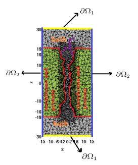
Figure 3: 2D cut plane y=0 for the mesh of gramicidin A single channel, where the green and grey parts shows the solute $\Omega_{m}$ and solvent domain $\Omega_{s}$ resepectively

Since it is difficult to find the analytical solution of (3.21)-(3.23), the result of simulation is compared with the experiment result via the current to observe the accuracy of the algorithms. The electric current is as follows ^{[3, 48]}

$$I=e\int_{\Omega_{I}}(J_{1}-J_{2})dS,$$ (3.24)

where ${\Omega_{I}}$ is any cross section of the channel, and the fluxes of positive and negative ions are defined by

$$J_{i}=-\nabla\cdot D_{i}\left(\nabla p^{i}+\frac{e}{K_{B}T}q^{i}p^{i}\nabla\phi\right),i=1,2.$$ (3.25)

The following two tables show the currents, and number of iterations and CPU time respectively by using Gummel iteration and algebraic FAS algorithm under different voltages. The experimental data was provided by Andersen ^[49].

Table 11: The current from the numerical simulation and experimental data at CsCl concentration 0.02M and different voltage(mV)

Voltage (mV)	Experimental data(pA)	Gummel results (pA)	FAS results (pA)
25	0.13	0.14	0.14
50	0.24	0.26	0.26
75	0.34	0.34	0.34
100	0.40	0.40	0.40
150	0.47	0.50	0.50
200	0.53	0.57	0.57
250	0.56	0.65	0.65
300	0.60	0.73	0.73
350	0.62	0.81	0.81
400	0.65	0.89	0.89

Table 12: Number of external iterations and the CPU time(s) for Gummel and FAS algorithms at CsCl concentration 0.02M and different voltage(mV)

Voltage(mV)	Gummel iteration number	FAS iteration number	Gummel CPU time	FAS CPU time
25	139	1	690	29
50	139	1	688	29
75	139	1	688	29
100	139	1	679	29
150	145	1	717	28
200	145	1	722	28
250	145	1	717	28
300	145	1	725	28
350	145	1	721	29
400	145	1	718	28

Remark 3.2.

One FAS iteration includes two rounds of pre-smoothing and post-smoothing respectively, and solving a coarse grid system once. Therefore, the time required to perform a FAS iteration is approximately six times that of a Gummel iteration.

From Tables 11 and 12, we can see FAS iteration runs much faster than Gummel iteration and the accuracy of them are similar.

Although the algebraic FAS method has better adaptability on unstructured or non-uniform grids, there are still defects such as insufficient adaptability to $L$ and excessive iteration for solving corresponding coarse grid nonlinear algebraic systems. Next, further improvements will be made based on the acceleration technique and adaptive method.

3.2 Improved algorithms based on the acceleration techniques and adaptive methods

First, we discuss some improved techniques for Gummel iteration. A natural idea is to use the under-relaxation technique ^{[50, 41]},

$$u^{new}=\alpha u^{new}+(1-\alpha)u^{old},$$ (3.26)

where the relaxation parameter $\alpha\in(0,1)$ is a preset constant. The corresponding Gummel iteration is described as follows.

Algorithm 3.5 Gummel iteration based on under-relaxation technique

S1.

Initialization. Given initial values $\phi_{h}^{(0)}=0,~{}p_{h}^{1,(0)}=0,~{}p_{h}^{2,(0)}=0$, iteration time $k=0$, parameter $\alpha$, tolerance $tol=1E-6$, maximum iteration number $M_{iter}=1000$.

S2.

Solve the linear equation

$$(\nabla\phi_{h}^{(k+1)},\nabla v_{h})=(f+p_{h}^{1,(k)}-p_{h}^{2,(k)},v_{h}),~{}\forall v_{h}\in V_{h}$$ (3.27)

to get $\phi_{h}^{(k+1)}$, and then let $\phi_{h}^{(k+1)}=\alpha\phi_{h}^{(k+1)}+(1-\alpha)\phi_{h}^{(k)}$.

S3.

Solve the linear equations

$$\left\{\begin{array}[]{ll}(\nabla p_{h}^{1,(k+1)},\nabla v_{h})+(p_{h}^{1,(k+1)}\nabla\phi_{h}^{(k+1)},\nabla v_{h})=(F^{1},v_{h}),&\forall v_{h}\in V_{h}\\ (\nabla p_{h}^{2,(k+1)},\nabla v_{h})-(p_{h}^{2,(k+1)}\nabla\phi_{h}^{(k+1)},\nabla v_{h})=(F^{2},v_{h}),&\forall v_{h}\in V_{h}\end{array}\right.$$ (3.28)

to get $p_{h}^{1,(k+1)}$ and $p_{h}^{2,(k+1)}$, and set $p_{h}^{1,(k+1)}=\alpha p_{h}^{1,(k+1)}+(1-\alpha)p_{h}^{1,(k)}$, $p_{h}^{2,(k+1)}=\alpha p_{h}^{2,(k+1)}+(1-\alpha)p_{h}^{2,(k)}$.

S4.

If $\|\phi_{h}^{(k+1)}-\phi_{h}^{(k)}\|_{L^{2}}\geq tol$ and $k\leq M_{iter}$, then $k=k+1$, and return to S2; otherwise output the numerical solution

$$\phi_{h}=\phi_{h}^{(k+1)},~{}p_{h}^{1}=p_{h}^{1,(k+1)},~{}p_{h}^{2}=p_{h}^{2,(k+1)}.$$

Next, we consider Example 3.1 to investigate the adaptability to convective intensity and convergence speed of the above algorithm. Set $\alpha=0.5$, $tol=1E-6$. Table 13 shows the numbers of iteration on uniform grids.

Table 13: Numbers of iterations

	$\sqrt{2.6}$	$\sqrt{2.7}$	$\sqrt{14.0}$	$\sqrt{15.0}$
$\frac{1}{16}$	20	20	21	*
$\frac{1}{32}$	19	19	19	*

where * represents divergence.

Comparing Table 13 with Table 4, it can be seen that Algorithm 3.5 indeed enhances its adaptability to $L$ (i.e. convective intensity), and the number of iterations does not change significantly with the scale, but there may be sudden instances of divergence. It may due to the fixation of values of $\alpha$. Hence, the following accelerated Gummel algorithm is provided to solve this problem.

3.2.1 Acceleration algorithms

Consider the following nonlinear algebraic system:

$$A(U)U=F,$$ (3.29)

where $A(U)$ and $F$ are order $n$ square matrix and vector, respectively.

Let $\hat{U}^{k}$ be the present iteration vector by using Gummel iteration to solve (3.29) and define the corresponding minimum problem

$$\min_{\alpha\in[0,1]}\|\alpha\hat{r}^{k}+(1-\alpha)r^{k-1}\|^{2}_{R^{n}},$$ (3.30)

where

$$\hat{r}^{k}=F-A(\hat{U}^{k})\hat{U}^{k},~{}~{}r^{k-1}=F-A(U^{k-1})U^{k-1}.$$ (3.31)

It is easy to know the minimum point is

$$\alpha^{*}=-\frac{b}{2a},~{}a=((\hat{r}^{k})^{T},\hat{r}^{k})+((r^{k-1})^{T},r^{k-1})-2((\hat{r}^{k})^{T},r^{k-1})\geq 0,$$ (3.32)

$$~{}b=2\big{(}((\hat{r}^{k})^{T},r^{k-1})-((r^{k-1})^{T},r^{k-1})\big{)}.$$ (3.33)

Updating $\hat{U}^{k}$ with $U^{k}$ using the parameter $\alpha^{*}$, we have

$$U^{k}=\hat{U}^{k}+(1-\alpha^{*})\hat{U}^{k-1}.$$ (3.34)

From the minimum problem (3.30) and (3.34), we get the following accelerated Gummel iteration.

Algorithm 3.6 Accelerated Gummel iteration-I

S1.

Initialization. Given initial value $\phi_{h}^{(0)}=0,~{}p_{h}^{1,(0)}=0,~{}p_{h}^{2,(0)}=0$, number of iterations $k=0$, stopping tolerance $tol=1E-6$, maximum iteration number $M_{iter}$=1000.

S2.

Solve linear equations

$$(\nabla\phi_{h}^{(k+1)},\nabla v_{h})=(f+p_{h}^{1,(k)}-p_{h}^{2,(k)},v_{h}),~{}~{}\forall v_{h}\in V_{h}$$ (3.35)

to get $\phi_{h}^{(k+1)}$.

S3.

Solve the following linear equations

$$\left\{\begin{array}[]{ll}(\nabla p_{h}^{1,(k+1)},\nabla v_{h})+(p_{h}^{1,(k+1)}\nabla\phi_{h}^{(k+1)},\nabla v_{h})=(F^{1},v_{h}),&\forall v_{h}\in V_{h}\\ (\nabla p_{h}^{2,(k+1)},\nabla v_{h})-(p_{h}^{2,(k+1)}\nabla\phi_{h}^{(k+1)},\nabla v_{h})=(F^{2},v_{h}),&\forall v_{h}\in V_{h}\end{array}\right.$$ (3.36)

to obtain $p_{h}^{1,(k+1)}$ and $p_{h}^{2,(k+1)}$.

S4.

If $k\geq 2$, then compute

$$r_{\phi}^{(k+1)}=(f+p_{h}^{1,(k+1)}-p_{h}^{2,(k+1)},\Psi)-(\nabla\phi_{h}^{(k+1)},\nabla\Psi).$$

From the minimum problem (3.30), we get $\alpha^{*}$, and then let $\phi_{h}^{(k+1)}=\alpha^{*}\phi_{h}^{(k+1)}+(1-\alpha^{*})\phi_{h}^{(k)}$, $p_{h}^{1,(k+1)}=\alpha^{*}p_{h}^{1,(k+1)}+(1-\alpha^{*})p_{h}^{1,(k)}$, $p_{h}^{2,(k+1)}=\alpha^{*}p_{h}^{2,(k+1)}+(1-\alpha^{*})p_{h}^{2,(k)}$.

S5.

If $|\phi_{h}^{(k+1)}-\phi_{h}^{(k)}\|_{L^{2}}\geq tol$ and $k\leq M_{iter}$ then set $k=k+1$ and return to S2, otherwise output the numerical solution

$$\phi_{h}=\phi_{h}^{(k+1)},~{}p_{h}^{1}=p_{h}^{1,(k+1)},~{}p_{h}^{2}=p_{h}^{2,(k+1)}.$$

Next, we investigate the adaptability to convective intensity and convergence speed of Algorithm 3.6 by taking Example 3.1 as an example. Let $tol=1E-6$. The following Table 14 shows the numbers of iterations on uniform meshes.

Table 14: Numbers of iteration of Algorithm 3.6

	$\sqrt{2.6}$	$\sqrt{2.7}$	$\sqrt{7.4}$	$\sqrt{7.5}$	$\sqrt{7.6}$	$\sqrt{7.7}$
$\frac{1}{16}$	9	9	16	18	21	–
$\frac{1}{32}$	9	9	18	–	–	–

Comparing Table 14 with Table 13, we can see that the number of itertion of Algorithm 3.6 is less than than that of Algorithm 3.5 in the convergent cases, but the adaptability to $L$ of it is worse than that of Algorithm 3.6.

Note that $\alpha^{*}$ is obtained by solving the minimum problem with respect to the residue of the Poisson equation. Hence, it may not be a good parameter for $p_{h}^{1}$ and $p_{h}^{2}$. To solve this problem, the combined $\phi_{h}^{(k+1)}$ is used to update $p_{h}^{1,(k+1)}$ and $p_{h}^{2,(k+1)}$. The detailed algorithm is as follows.

Algorithm 3.7 Accelerated Gummel iteration-II

S1.

Initialization. Given initial value $\phi_{h}^{(0)}=0,~{}p_{h}^{1,(0)}=0,~{}p_{h}^{2,(0)}=0$, number of iteration $k=0$, stopping tolerace $tol=1E-6$, maximum itertion number $M_{iter}$=1000.

S2.

Solve the linear equation

$$(\nabla\phi_{h}^{(k+1)},\nabla v_{h})=(f+p_{h}^{1,(k)}-p_{h}^{2,(k)},v_{h}),~{}~{}\forall v_{h}\in V_{h}$$ (3.37)

to get $\phi_{h}^{(k+1)}$.

S3.

Solve the linear equations

$$\left\{\begin{array}[]{ll}(\nabla p_{h}^{1,(k+1)},\nabla v_{h})+(p_{h}^{1,(k+1)}\nabla\phi_{h}^{(k+1)},\nabla v_{h})=(F^{1},v_{h}),&\forall v_{h}\in V_{h},\\ (\nabla p_{h}^{2,(k+1)},\nabla v_{h})-(p_{h}^{2,(k+1)}\nabla\phi_{h}^{(k+1)},\nabla v_{h})=(F^{2},v_{h}),&\forall v_{h}\in V_{h}\end{array}\right.$$ (3.38)

to obtain $p_{h}^{1,(k+1)}$ and $p_{h}^{2,(k+1)}$.

S4.

If $k\geq 2$, then compute

$$r_{\phi}^{(k+1)}=(f+p_{h}^{1,(k+1)}-p_{h}^{2,(k+1)},\Psi)-(\nabla\phi_{h}^{(k+1)},\nabla\Psi),$$

and solve the minimum problem (3.30) to get $\alpha^{*}$. Set $\phi_{h}^{(k+1)}=\alpha^{*}\phi_{h}^{(k+1)}+(1-\alpha^{*})\phi_{h}^{(k)}$, and repeat Step S3 to obtain $n_{h}^{(k+1)},p_{h}^{(k+1)}$.

S5.

If $\|\phi_{h}^{(k+1)}-\phi_{h}^{(k)}\|_{L^{2}}\geq tol$ and $k\leq M_{iter}$, then set $k=k+1$, return to S2, otherwise output the following solution

$$\phi_{h}=\phi_{h}^{(k+1)},~{}p_{h}^{1}=p_{h}^{1,(k+1)},~{}p_{h}^{2}=p_{h}^{2,(k+1)}.$$

Now, we still use Example 3.1 to investigate the adaptability to convective intensity and convergence speed of Algorithm 3.7. Table 15 shows the numbers of iterations on uniform meshes.

Table 15: Numbers of iteration of Algorithm 3.7

	$\sqrt{2.6}$	$\sqrt{2.7}$	$\sqrt{10}$	$\sqrt{11}$	$\sqrt{12}$	$\sqrt{13}$	$\sqrt{14}$
$\frac{1}{16}$	3	3	19	39	110	398	$>$1000
$\frac{1}{32}$	3	3	19	43	132	523	$>$1000

Comparing Table 15 with Table 4, we know that Algorithm 3.7 indeed accelerates convergence speed and can calculate larger $L$. For example, the approximate upper limit of $L$ that the Gummel iteration can calculate is about $L=\sqrt{2.7}$ when $h=\frac{1}{16}$, while that is more than $L=\sqrt{13}$ for Algorithm 3.7, and the number of iteration of Gummel algorithm is about $39$ times that of Algorithm 3.7 when $L=\sqrt{2.6}$.

The above acceleration techniques have improved the adaptability to size $L$ in a certain extent, but when $L$ increases to a certain value, there are also a rapid increase in iteration numbers and slow convergence speed. It is observed that $\alpha^{*}$ is very small at the first iteration and becomes larger as the decline of the residual. For instance, in the case of $L=\sqrt{11}$, the magnitude of $\alpha^{*}$ is $1E-3$ when the number of iteration is smaller, while it is $1E-1$ at the last few steps. Considering this phenomenon, we present a adaptive Gummel iteration as follows.

3.2.2 An adaptive algorithm

Algorithm 3.8 Adaptive Gummel iteration

S1.

Setting $M_{iter}=2$, and given $\theta_{\alpha}$ and $\alpha$ , call Algorithm 3.7 to get $\alpha^{*}$.

S2.

If $\alpha^{*}\geq\theta_{\alpha}$, then use Algorithm 3.7 directly to solve the algebraic system, otherwise go to S3.

S3.-S4.

Same as Steps S1-S2 in Algorithm 3.7.

S5.

If $k=1$, then set $\phi_{h}^{(k+1)}=\alpha\phi_{h}^{(k+1)}+(1-\alpha)\phi_{h}^{(k)}$, and solve linear equation  (3.38) to get $p_{h}^{1,(k+1)}$ and $p_{h}^{2,(k+1)}$, otherwise compute

$$r_{\phi}^{(k+1)}=(p_{h}^{1,(k+1)}-p_{h}^{2,(k+1)},\nabla\Psi)-(\nabla\phi_{h}^{(k+1)},\nabla\Psi),$$ (3.39)

$$uc=\frac{\|\phi_{h}^{(k+1)}-\phi_{h}^{(k)}\|_{L^{2}}}{\|\phi_{h}^{(k)}\|_{L^{2}}},$$ (3.40)

and obtain $\alpha^{*}$ from the minimum problem (3.30). Then given $(\theta_{1}^{i},\theta_{2}^{i}),i=1,\dots,m$, call Algorithm 3.9 to update $\phi_{h}^{(k+1)}$, $p_{h}^{1,(k+1)}$ and $p_{h}^{2,(k+1)}$.

S6.

Compute

$$r^{(k+1)}=(r_{\phi}^{(k+1)},r_{p^{1}}^{(k+1)},r_{p^{2}}^{(k+1)}),$$

where

$$r_{p_{h}^{i}}^{(k+1)}=(F^{i},v_{h})-(\nabla p_{h}^{i,(k+1)},\nabla v_{h})+(p_{h}^{i,(k+1)}\nabla\phi_{h}^{(k+1)},\nabla v_{h}),~{}i={1},{2}.$$

If $\|r^{(k+1)}\|_{L^{2}}\geq tol$ and $k\leq M_{iter}$, then $k=k+1$ and return to S3, otherwise

$$\phi_{h}=\phi_{h}^{(k+1)},~{}p_{h}^{2}=p_{h}^{2,(k+1)},~{}p_{h}^{1}=p_{h}^{1,(k+1)}.$$

Algorithm 3.9 Algorithm of updating $\phi_{h}^{(k+1)},~{}p_{h}^{1,(k+1)},~{}p_{h}^{2,(k+1)}$

S1. Update $\phi_{h}^{(k+1)}$

.

S1.1

If $\|r^{(k)}\|_{L^{2}}\in(r_{1},+\infty)$ and $uc\in[\theta_{1}^{1},\theta_{2}^{1}]$, goto S2, otherwise

S1.1

Setting $\hat{\phi}_{h}^{(k+1)}=\alpha^{*}\phi_{h}^{(k+1)}+(1-\alpha^{*})\phi_{h}^{(k)}$, compute $\hat{uc}=\frac{\|\hat{\phi}_{h}^{(k+1)}-\phi_{h}^{(k)}\|_{L^{2}}}{\|\phi_{h}^{(k)}\|_{L^{2}}}$.

S1.2

If $\hat{uc}<1e-10$, then take $\alpha^{*}=0.5$ and return to S1.1.

If $1e-10\leq\hat{uc}<\theta_{1}^{1}$, then $\alpha^{*}=2{\alpha}^{*}$ and return to S1.1.

If $\hat{uc}\in[\theta_{1}^{1},\theta_{2}^{1}]$, then set $\phi_{h}^{(k+1)}=\hat{\phi}_{h}^{(k+1)}$, goto S2.

If $\hat{uc}>\theta_{2}^{1}$, then set $\alpha^{*}={\alpha^{*}}/{2}$, and return to S1.1.

$\cdot$

$\cdot$

$\cdot$

S1.m

If $\|r^{(k)}\|_{L^{2}}\in(r_{m},r_{m-1}]$ and $uc\in[\theta_{1}^{m},\theta_{2}^{m}]$, then goto S2, otherwise repeat steps S1.1-S1.2, in which $\theta_{1}^{1}$ and $\theta_{2}^{1}$ are considered as $\theta_{1}^{m}$ and $\theta_{2}^{m}$, respectively.

S2. (Update $p_{h}^{1,(k+1)},p_{h}^{2,(k+1)}$)

Solve (3.38) to get $p_{h}^{1,(k+1)}$ and $p_{h}^{2,(k+1)}$.

Next we use Example 3.1 as an example to observe the adaptability to convective intensity and convergence speed of algorithm 3.8. The parameters in Algorithm 3.8 are taken as follows:

$$tol=1E-6,~{}\alpha=0.1,~{}\theta_{\alpha}=1e-3,~{}m=3,~{}r_{1}=1e-3,~{}r_{2}=1e-4,~{}r_{3}=1e-6,$$ (3.41)

$$(\theta_{1}^{1},\theta_{2}^{1})=(1e-1,5e-1),~{}(\theta_{1}^{2},\theta_{2}^{2})=(1e-2,1e-1),~{}(\theta_{1}^{3},\theta_{2}^{3})=(0,100).$$

Table 16 shows the numbers of iteration of Algorithm 3.8 on uniform meshes.

Table 16: numbers of iteration of Algorithm 3.8

	$\sqrt{2.7}$	$\sqrt{2.8}$	$\sqrt{10}$	$\sqrt{11}$	$\sqrt{12}$	$\sqrt{13}$	$\sqrt{14}$	$\sqrt{15}$	$\sqrt{18}$	$\sqrt{19}$	$\sqrt{20}$	$\sqrt{25}$
$\frac{1}{16}$	3	3	10	12	12	13	14	16	17	–	–	–
$\frac{1}{32}$	3	3	17	16	13	17	24	30	29	27	26	–

It can be seen by comparing the results of Tables 15-16 that the adaptability to $L$ of Algorithm 3.8 is better than that of Algorithm 3.7. For example, the approximate upper limit of $L$ that Algorithm 3.7 can calculate is about $L=\sqrt{14}$ when $h=\frac{1}{16}$, while that is more than $L=\sqrt{18}$ for Algorithm 3.8, and the number of iterations of it is not more than that of Algorithm 3.7. In order to further improve the adaptability to $L$, we adjust the values of parameters as follows:

$$tol=1E-6,~{}\alpha=0.1,~{}\theta_{\alpha}=1e-3,$$ (3.42)

$$~{}m=3,~{}r_{1}=1e-2,~{}r_{2}=1e-3,~{}r_{3}=1e-5,~{}r_{4}=1e-6,$$

$$(\theta_{1}^{1},\theta_{2}^{1})=(1e-1,5e-1),~{}(\theta_{1}^{2},\theta_{2}^{2})=(1e-2,1e-1),~{}(\theta_{1}^{3},\theta_{2}^{3})=(1e-4,1e-3)$$

$$(\theta_{1}^{4},\theta_{2}^{4})=(1e-5,1e-4),$$

and show the results on Table 17.

Table 17: Numbers of iterations of Algorithm 3.8 after parameter adjustment

	$\sqrt{18}$	$\sqrt{19}$	$\sqrt{20}$	$\sqrt{25}$	$\sqrt{30}$	$\sqrt{35}$	$\sqrt{40}$
$\frac{1}{16}$	116	113	108	47	151	153	–

It is seen from Tables 16 and 17 that the size $L$ that Algorithm 3.8 can calculate can be larger if $m$ is increased and $\theta_{1}^{\eta},\theta_{2}^{\eta}$ is decreased.

It should be pointed out that the improved algorithms based on the acceleration technique and the adaptive method in this section are designed for the Gummel iterations an example. However, these algorithms essentially do not require modifications and can be directly applied to the FAS algorithm.

4 Conclusion

In this paper, we study several fast algorithms for EAFE nonlinear discrete systems to solve a class of general time-dependent PNP equations. To overcome the drawbacks such as slow convergence speed of the Gummel iteration, a geometric FAS algorithm is proposed to improve the solving efficiency. Then, an algebraic FAS algorithm is designed to improve the limitations such as the requirement of nested coarse grids of the geometric FAS algorithm. The numerical experiments including practical PNP equations in ion channel show that algebraic FAS can improve the efficiency of decoupling external iterations and expand the size of domain can solved compared with the classical Gummel iteration. Finally, the improved algorithms based on the acceleration technique and adaptive method to solve the problem of excessive coarse grid iterations in FAS algorithms when convective intensity is high. Numerical experiments have shown that the improved algorithms converge faster and significantly enhance the adaptability of convective intensity. These fast algorithms presented in this paper is easy to extend to other FE nonlinear discrete systems, such as classical FE and SUPG method etc. It is promising to apply them to more complex PNP models, such as PNP equations in more complex ion channels and semiconductor devices.

Acknowledgement S. Shu was supported by the China NSF (NSFC 12371373). Y. Yang was supported by the China NSF (NSFC 12161026).

References

- [1] Walther Nernst. Die elektromotorische wirksamkeit der jonen. Zeitschrift für physikalische Chemie, 4(1):129–181, 1889.
- [2] Max Planck. Ueber die erregung von electricität und wärme in electrolyten. Annalen Der Physik, 275(2):161–186, 1890.
- [3] Bin Tu, Minxin Chen, Yan Xie, Linbo Zhang, Bob Eisenberg, and Benzhuo Lu. A parallel finite element simulator for ion transport through three-dimensional ion channel systems. Journal of Computational Chemistry, 34(24):2065–2078, 2013.
- [4] Bob Eisenberg. Ionic channels in biological membranes-electrostatic analysis of a natural nanotube. Contemporary Physics, 39(6):447–466, 1998.
- [5] Amit Singer and John Norbury. A Poisson-Nernst-Planck model for biological ion channels-An asymptotic analysis in a three-dimensional narrow funnel. SIAM Journal on Applied Mathematics, 70(3):949–968, 2009.
- [6] Peter A. Markowich. The stationary semiconductor device equations. Springer Science & Business Media, 1985.
- [7] France Brezzi, Luisa Donatella Marini, Stefano Micheletti, Paola Pietra, Riccardo Sacco, and Song Wang. Discretization of semiconductor device problems (I). Handbook of Numerical Analysis, 13:317–441, 2005.
- [8] John James Henry Miller, Wil Schilders, and Song Wang. Application of finite element methods to the simulation of semiconductor devices. Reports on Progress in Physics, 62(3):277, 1999.
- [9] Jingjie Xu, Benzhuo Lu, and Linbo Zhang. A time-dependent finite element algorithm for simulations of ion current rectification and hysteresis properties of 3D nanopore system. IEEE Transactions on Nanotechnology, 17(3):513–519, 2018.
- [10] Hirofumi Daiguji, Peidong Yang, and Arun Majumdar. Ion transport in nanofluidic channels. Nano Letters, 4(1):137–142, 2004.
- [11] Benzhuo Lu, Michael J. Holst, J. Andrew McCammon, and YongCheng Zhou. Poisson-Nernst-Planck equations for simulating biomolecular diffusion-reaction processes I: Finite element solutions. Journal of Computational Physics, 229(19):6979–6994, 2010.
- [12] Dexuan Xie and Benzhuo Lu. An effective finite element iterative solver for a Poisson-Nernst-Planck ion channel model with periodic boundary conditions. SIAM Journal on Scientific Computing, 42(6):B1490–B1516, 2020.
- [13] Jinyong Ying, Ronghong Fan, Jiao Li, and Benzhuo Lu. A new block preconditioner and improved finite element solver of Poisson-Nernst-Planck equation. Journal of Computational Physics, 430:110098, 2021.
- [14] Ying Yang, Ming Tang, Chun Liu, Benzhuo Lu, and Liuqiang Zhong. Superconvergent gradient recovery for nonlinear Poisson-Nernst-Planck equations with applications to the ion channel problem. Advances in Computational Mathematics, 46:1–35, 2020.
- [15] Alfredo E Cardenas, Rob D Coalson, and Maria G Kurnikova. Three-dimensional Poisson-Nernst-Planck theory studies: Influence of membrane electrostatics on gramicidin A channel conductance. Biophysical Journal, 79(1):80–93, 2000.
- [16] Hailiang Liu and Zhongming Wang. A free energy satisfying finite difference method for Poisson-Nernst-Planck equations. Journal of Computational Physics, 268:363–376, 2014.
- [17] Allen Flavell, Michael Machen, Bob Eisenberg, Julienne Kabre, Chun Liu, and Xiaofan Li. A conservative finite difference scheme for Poisson-Nernst-Planck equations. Journal of Computational Electronics, 13:235–249, 2014.
- [18] Dongdong He and Kejia Pan. An energy preserving finite difference scheme for the Poisson-Nernst-Planck system. Applied Mathematics and Computation, 287:214–223, 2016.
- [19] Claire Chainais-Hillairet and Yue-Jun Peng. Finite volume approximation for degenerate drift-diffusion system in several space dimensions. Mathematical Models and Methods in Applied Sciences, 14(03):461–481, 2004.
- [20] Claire Chainais-Hillairet and Yue-Jun Peng. Convergence of a finite-volume scheme for the drift-diffusion equations in 1D. IMA Journal of Numerical Analysis, 23(1):81–108, 2003.
- [21] Claire Chainais-Hillairet, Jian-Guo Liu, and Yue-Jun Peng. Finite volume scheme for multi-dimensional drift-diffusion equations and convergence analysis. ESAIM: Mathematical Modelling and Numerical Analysis, 37(2):319–338, 2003.
- [22] Marianne Bessemoulin-Chatard, Claire Chainais-Hillairet, and Marie Helene Vignal. Study of a finite volume scheme for the drift-diffusion system. Asymptotic behavior in the quasi-neutral limit. SIAM Journal on Numerical Analysis, 52(4):1666–1691, 2014.
- [23] Qianru Zhang, Qin Wang, Linbo Zhang, and Benzhuo Lu. An inverse averaging finite element method for solving three-dimensional Poisson-Nernst-Planck equations in nanopore system simulations. The Journal of Chemical Physics, 155(19), 2021.
- [24] Linbo Zhang Qin Wang, Hongliang Li and Benzhuo Lu. A stabilized finite element method for the Poisson-Nernst-Planck equation in three-dimensional ion channel simulations. Applied Mathematics Letters, 111:106652, 2021.
- [25] Bin Tu, Yan Xie, Linbo Zhang, and Benzhuo Lu. Stabilized finite element methods to simulate the conductances of ion channels. Computer Physics Communications, 188:131–139, 2015.
- [26] Qianru Zhang, Qin Wang, Linbo Zhang, and Benzhuo Lu. A class of finite element methods with averaging techniques for solving the three-dimensional drift-diffusion model in semiconductor device simulations. Journal of Computational Physics, 458:111086, 2022.
- [27] Sanjay R. Mathur and Jayathi Y. Murthy. A multigrid method for the Poisson-Nernst-Planck equations. International Journal of Heat and Mass Transfer, 52(17-18):4031–4039, 2009.
- [28] Arthur Bousquet, Xiaozhe Hu, Maximilian S. Metti, and Jinchao Xu. Newton solvers for drift-diffusion and electrokinetic equations. SIAM Journal on Scientific Computing, 40(3):B982–B1006, 2018.
- [29] Jicheng Jin, Shi Shu, and Jinchao Xu. A two-grid discretization method for decoupling systems of partial differential equations. Mathematics of Computation, 75(256):1617–1626, 2006.
- [30] Ruigang Shen, Shi Shu, Ying Yang, and Benzhuo Lu. A decoupling two-grid method for the time-dependent Poisson-Nernst-Planck equations. Numerical Algorithms, 83:1613–1651, 2020.
- [31] Achi Brandt. Multi-level adaptive solutions to boundary-value problems. Mathematics of Computation, 31(138):333–390, 1977.
- [32] Haim Waisman and Jacob Fish. A heterogeneous space–time full approximation storage multilevel method for molecular dynamics simulations. International Journal for Numerical Methods in Engineering, 73(3):407–426, 2008.
- [33] Jun Liu, Brittany D. Froese, Adam M. Oberman, and Mingqing Xiao. A multigrid scheme for 3D Monge-Ampère equations. International Journal of Computer Mathematics, 94(9):1850–1866, 2017.
- [34] Wenqiang Feng, Zhenlin Guo, John S. Lowengrub, and Steven M. Wise. A mass-conservative adaptive FAS multigrid solver for cell-centered finite difference methods on block-structured, locally-cartesian grids. Journal of Computational Physics, 352:463–497, 2018.
- [35] Mark F. Adams, Ravi Samtaney, and Achi Brandt. Toward textbook multigrid efficiency for fully implicit resistive magnetohydrodynamics. Journal of Computational Physics, 229(18):6208–6219, 2010.
- [36] Achi Brandt and Oren E. Livne. Multigrid Techniques: 1984 Guide with Applications to Fluid Dynamics, Revised Edition. SIAM, 2011.
- [37] William L. Briggs, Van Emden Henson, and Steve F. McCormick. A multigrid tutorial. SIAM, 2000.
- [38] Achi Brandt and Oren E. Livne. Full approximation scheme (FAS) and applications. In Multigrid Techniques: 1984 Guide With Applications To Fluid Dynamics, pages 87–97. SIAM, 2011.
- [39] Mhamad Mahdi Alloush, Marwan Darwish, Fadl Moukalled, and Luca Mangani. The development of preliminary modifications for an improved full approximation storage method in pressure-based flow solvers. In AIP Conference Proceedings, volume 2425. AIP Publishing, 2022.
- [40] Philipp Birken, Jonathan Bull, and Antony Jameson. Preconditioned smoothers for the full approximation scheme for the RANS equations. Journal of Scientific Computing, 78:995–1022, 2019.
- [41] Benzhuo Lu, YongCheng Zhou, Gary A Huber, Stephen D Bond, Michael Holst, and J. Andrew McCammon. Electrodiffusion: A continuum modeling framework for biomolecular systems with realistic spatiotemporal resolution. The Journal of chemical physics, 127(13), 2007.
- [42] Yang Liu, Shi Shu, Huayi Wei, and Ying Yang. A virtual element method for the steady-state Poisson-Nernst-Planck equations on polygonal meshes. Computers & Mathematics with Applications, 102:95–112, 2021.
- [43] Herbert Gajewski and Konrad Gröger. On the basic equations for carrier transport in semiconductors. Journal of Mathematical Analysis and Applications, 113(1):12–35, 1986.
- [44] Ed Bueler. The full approximation storage multigrid scheme: A 1D finite element example. arXiv preprint arXiv:2101.05408, 2021.
- [45] John W. Ruge and Klaus Stüben. Algebraic multigrid. pages 73–130, 1987.
- [46] David S. Kershaw. Differencing of the diffusion equation in Lagrangian hydrodynamic codes. Journal of Computational Physics, 39(2):375–395, 1981.
- [47] Minxin Chen and Benzhuo Lu. TMSmesh: A robust method for molecular surface mesh generation using a trace technique. Journal of Chemical Theory and Computation, 7(1):203–212, 2011.
- [48] Benzhuo Lu and Yongcheng Zhou. Poisson-Nernst-Planck equations for simulating biomolecular diffusion-reaction processes II: Size effects on ionic distributions and diffusion-reaction rates. Biophysical Journal, 100(10):2475–2485, 2011.
- [49] Olaf S. Andersen. Ion movement through gramicidin A channels. interfacial polarization effects on single-channel current measurements. Biophysical Journal, 41(2):135–146, 1983.
- [50] Wolfgang Nonner, Dirk Gillespie, Douglas Henderson, and Bob Eisenberg. Ion accumulation in a biological calcium channel: effects of solvent and confining pressure. The Journal of Physical Chemistry B, 105(27):6427–6436, 2001.