An Attentive Inductive Bias for Sequential Recommendation
Beyond the Self-Attention

Abstract

Sequential recommendation (SR) models based on Transformers have achieved remarkable successes. The self-attention mechanism of Transformers for computer vision and natural language processing suffers from the oversmoothing problem, i.e., hidden representations becoming similar to tokens. In the SR domain, we, for the first time, show that the same problem occurs. We present pioneering investigations that reveal the low-pass filtering nature of self-attention in the SR, which causes oversmoothing. To this end, we propose a novel method called Beyond Self-Attention for Sequential Recommendation (BSARec), which leverages the Fourier transform to i) inject an inductive bias by considering fine-grained sequential patterns and ii) integrate low and high-frequency information to mitigate oversmoothing. Our discovery shows significant advancements in the SR domain and is expected to bridge the gap for existing Transformer-based SR models. We test our proposed approach through extensive experiments on 6 benchmark datasets. The experimental results demonstrate that our model outperforms 7 baseline methods in terms of recommendation performance.

1 Introduction

Recommender systems play a vital role in web applications, delivering personalized item recommendations by analyzing user-item interactions (He et al. 2020; Choi, Jeon, and Park 2021; Kong et al. 2022; Hong et al. 2022; Choi et al. 2023a; Gao et al. 2023). As users’ preferences evolve over time, capturing the temporal user behavior becomes essential. This is where SR steps in, attracting substantial research attention (Hidasi et al. 2016; Wu et al. 2022; Gao et al. 2023; Tang and Wang 2018; Kang and McAuley 2018; Chen et al. 2019; Schedl et al. 2018; Hansen et al. 2020; Jiang et al. 2016; Huang et al. 2018).

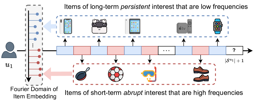
Figure 1: Illustration of high and low-frequency signals in SR. A user $u_{1}$’s long-term persisting interests and tastes constitute low frequencies in the Fourier domain of embedding, and abrupt short-term changes in $u_{1}$’s interests correspond to high frequencies.

Method	Inductive Bias	Self-Attention	High-pass Filter
SASRec	✗	✓	✗
BERT4Rec	✗	✓	✗
FMLPRec	✓	✗	✗
DuoRec	✗	✓	✗
BSARec	✓	✓	✓

Table 1: Comparison of existing Transformer-based methods that differ at three points: i) using inductive bias, ii) using self-attentions, and iii) using high-pass filters

With the increasing popularity of sequential recommendation (SR) systems, Transformer-based models, especially those utilizing self-attention (Vaswani et al. 2017), have emerged as dominant approaches for providing accurate and personalized recommendations to users (Kang and McAuley 2018; Sun et al. 2019; Li, Wang, and McAuley 2020; Wu et al. 2020; Wu, Cai, and Wang 2020). However, despite their successes in the SR, Transformer-based models possess inherent limitations that confine themselves to the learned self-attention matrix. The following two key limitations need to be addressed: i) First, the models may still suffer from suboptimal performance due to the insufficient inductive bias inherent in processing sequences with self-attention (Dosovitskiy et al. 2020). While the self-attention mechanism captures long-range dependencies, it may not only adequately consider certain fine-grained sequential patterns but also be overfitted to training data, leading to potential weak generalization capabilities. As Table 1 shows, SASRec (Kang and McAuley 2018), BERT4Rec (Sun et al. 2019), and DuoRec (Qiu et al. 2022) rely on training the self-attention layer and lack inductive bias. ii) The second limitation pertains to the low-pass filtering nature of self-attention. By focusing on the entire range of data, self-attention may unintentionally smoothen out important and detailed patterns in embedding, resulting the oversmoothing problem. The oversmoothing issue poses a significant challenge in the SR domain, as it may hinder the ability of model to capture crucial temporal dynamics and provide accurate predictions. In Table 1, most Transformer-based models are limited to low-pass filters. These models do not consider high-pass filters. Note that FMLPRec (Zhou et al. 2022) attempts to learn a filter, but it tends to gravitate towards the low-pass filter (cf. Fig. 2 (b)). As shown in Fig. 1, the low-pass filter only captures the ongoing preferences of the user i.e. an Apple fanatic, and it may be difficult to capture preferences based on new interests or trends (e.g., snorkel mask to buy for vacation). When recommending items for the next time ($|\mathcal{S}^{u_{1}}|+1$), it is undemanding to recommend long-term interests, but recommending short-term interests is a challenging task.

In this paper, we address these two limitations and present Beyond Self-Attention for Sequential Recommendation (BSARec), a novel model that uses inductive bias via Fourier transform with self-attention. By using the Fourier transform, BSARec gains access to the inductive bias of frequency information, enabling the capture of essential patterns and periodicity that may be overlooked by self-attention alone. This enhances the inductive bias and has the potential to improve recommendation performance.

To tackle the oversmoothing issue, we introduce our own designed frequency rescaler to apply high-pass filters into BSARec’s architecture. Our frequency rescaler can capture high-frequency behavioral patterns, such as interests driven by short-term trends, as well as low-frequency patterns, such as long-term interests, in a user’s behavioral patterns (cf. Fig. 1). Additionally, our method provides a perspective to improve the performance of SR models and solve the problem of oversmoothing.

To evaluate the efficacy of BSARec, we conduct extensive experiments on 6 benchmark datasets. Our experimental results demonstrate that BSARec consistently outperforms 7 baseline methods regarding recommendation performance. Additionally, we conduct a series of experiments that underscore the necessity of our approach and verify its effectiveness in mitigating the oversmoothing problem, leading to improved recommendation accuracy and enhanced generalization capabilities. The contributions of this work are as follows:

• We unveil the low-pass filtering nature of the self-attention of Transformer-based SR models, resulting in the problem of oversmoothing.

• We propose a novel model, Beyond Self-Attention for Sequential Recommendation (BSARec), that leverages the Fourier transform to balance between our inductive bias and self-attention. Further, we design the rescaler for high-pass filters to mitigate the oversmoothing issue.

• Extensive evaluation on 6 benchmark datasets demonstrates BSARec’s outperformance over 7 baseline methods, validating its effectiveness in improving recommendation performance.

2 Preliminaries

2.1 Problem Formulation

The goal of SR is to predict the user’s next interaction with an item given their historical interaction sequences. Given a set of users $\mathcal{U}$ and items $\mathcal{V}$, we can sort the interacted items of each user $u\in\mathcal{U}$ chronologically in a sequence as $\mathcal{S}^{u}=[v^{u}_{1},v^{u}_{2},\ldots v^{u}_{|\mathcal{S}^{u}|}]$, where $v^{u}_{i}$ denotes the $i$-th interacted item in the sequence. The aim is to recommend a Top-$k$ list of items as potential next items in a sequence. Formally, we predict $p(v^{u}_{|\mathcal{S}^{u}|+1}=v|\mathcal{S}^{u})$.

2.2 Self-Attention for Sequential Recommendation

The basic idea behind the self-attention mechanism is that elements within sequences are correlated but hold varying levels of significance concerning their positions in the sequence. Self-attention uses dot-products between items in the sequence to infer their correlations, which are defined as follows:

$$\mathbf{A}=\textrm{softmax}\left(\frac{\mathbf{Q}\mathbf{K}^{\mathtt{T}}}{\sqrt{d}}\right),$$ (1)

where $\mathbf{Q}=\mathbf{E}_{\mathcal{S}^{u}}\mathbf{W}_{Q}$, $\mathbf{K}=\mathbf{E}_{\mathcal{S}^{u}}\mathbf{W}_{K}$, and $d$ is the scale factor. The scaled dot-product component learn the latent correlation between items. Other components in Transformer are utilized in SASRec, including the point-wise feed-forward network, residual connection, and layer normalization. Our method uses this self-attention matrix and adds an inductive bias to find the trade-off between the two methods.

2.3 Discrete vs. Graph Fourier Transform

This subsection introduces the concept of the frequency domain and the Fourier transform, providing a cohesive foundation for the proposed method.

The Discrete Fourier Transform (DFT) is a linchpin in digital signal processing (DSP), projecting a sequence of values into the frequency domain (or the Fourier domain). We typically use $\mathcal{F}:\mathbb{R}^{N}\rightarrow\mathbb{C}^{N}$ to denote the Discrete Fourier Transform (DFT) with the Inverse DFT (IDFT) $\mathcal{F}^{-1}:\mathbb{C}^{N}\rightarrow\mathbb{R}^{N}$. Applying $\mathcal{F}$ to a signal is equal to multiplying it from the left by a DFT matrix. The rows of this matrix consist of the Fourier basis $\bm{f}_{j}=[e^{2\pi i(j-1)\cdot 0}\ldots e^{2\pi i(j-1)(N-1)}]^{\mathtt{T}}/\sqrt{N}\in\mathbb{R}^{N}$, where $i$ is the imaginary unit and $j$ denotes the $j$-th row. For the spectrum of $\bm{x}$, let it be represented as $\widetilde{\bm{x}}=\mathcal{F}\bm{x}$. We can define $\widetilde{\bm{x}}_{\text{lfc}}\in\mathbb{C}^{c}$ containing the $c$ lowest elements of $\widetilde{\bm{x}}$, and $\widetilde{\bm{x}}_{\text{hfc}}\in\mathbb{C}^{N-c}$ as the vector containing the remaining elements. The low-frequency components (LFC) of the sequence signal $\bm{x}$ are defined as:

$$\text{LFC}[\bm{x}]=\left[\bm{f}_{1},\bm{f}_{2},\ldots,\bm{f}_{c}\right]\widetilde{\bm{x}}_{\text{lfc}}\in\mathbb{R}^{N}.$$ (2)

Conversely, the high-frequency components (HFC) are:

$$\text{HFC}[\bm{x}]=\left[\bm{f}_{c+1},\bm{f}_{c+2},\ldots,\bm{f}_{N}\right]\widetilde{\bm{x}}_{\text{hfc}}\in\mathbb{R}^{N}.$$ (3)

Note that we use real-valued DFT and multiplying with the Fourier bases in Eqs. 2 and 3 means IDFT. For more descriptions, interested readers should refer to Appendix.

The Graph Fourier Transform (GFT) can be considered as a generalization of DFT toward graphs. In other words, DFT is a special case of GFT, where a ring graph of $N$ nodes is used (see Fig. 2 (a)) (Sandryhaila and Moura 2014). In fact, DFT is a method to project a sequence of values onto the eigenspace of the Laplacian matrix of the ring graph (which is the same as the Fourier domain).

The frequency concept can also be described with the ring graph. The number of neighboring nodes with different signs on their signals corresponds to the frequency. Therefore, low-frequency information means a series of signals over $N$ nodes whose signs do not change often. In the case of the SR in our work, where $N$ nodes mean $N$ item embeddings, such low-frequency information means a long-standing interest of a user (see. Fig. 1).

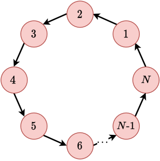
(a) A ring graph

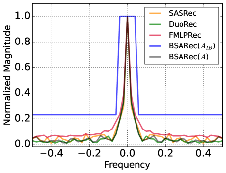
(b) Spectral responses

Figure 2: (a) A ring graph with $N$ nodes, and (b) visualization of the filter of the self-attentions in LastFM.

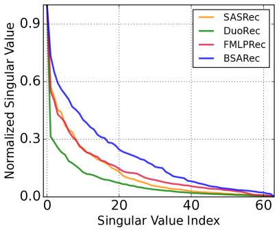
(a) Singular value

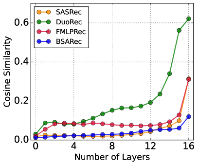
(b) Cosine similarity

Figure 3: Visualization of oversmoothing in LastFM. The singular values and cosine similarity of user sequence output embedding.

3 Motivation

In this section, we show that self-attention in the spectral domain is a low-pass filter that continuously erases high-frequency information. We visualize the spectrum of self-attention of the Transformer-based sequantial model as shown in the Fig. 2 (b). It shows the spectrum is concentrated in the low frequency region, and reveals that self-attention is a low-pass filter. We further make theoretical justifications for the low-pass filter of self-attention.

Theorem 3.1 (Self-Attention is a low-pass filter).

Let $\mathbf{A}=\textrm{softmax}(\mathbf{Q}\mathbf{K}^{\mathtt{T}}/\sqrt{d})$. Then $\mathbf{A}$ inherently acts as a low-pass filter. For all $\bm{x}\in\mathbb{R}^{N}$, in other words, $\lim_{t\rightarrow\infty}||\text{HFC}[\mathbf{A}^{t}(\bm{x})]||_{2}/||\text{LFC}[\mathbf{A}^{t}(\bm{x})]||_{2}=0$ (See Appendix for the formal definition of the low-pass filter).

Theorem 3.1 is ensured by the Perron-Frobenius theorem (Meyer and Stewart 2023; He and Wai 2021) and it reveals that the attention matrix is always a low pass filter independent of the input key and query matrices. A proof is provided in Appendix. If the self-attention matrix is applied successively, the final output loses all feature expressiveness as the number of layers increases to infinity.

Therefore, the self-attention causes the oversmoothing problem that Tranformer-based sequential models lose feature representation in deep layers (see Fig. 3). As can be seen from the empirical analysis of Fig. 3, as the number of layers of these models increases, the cosine similarity increases and the singular value tends to decay rapidly  (Fan et al. 2023). This inevitably causes the model to fail to capture the user’s detailed preferences, and performance degradation is a natural result.

We not only alleviate oversmoothing using a high-pass filter as motivation against this background, but also try to capture short-term preferences of user behavior patterns through inductive bias.

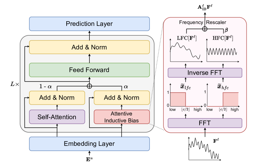
Figure 4: Architecture of the proposed BSARec. We propose a BSA encoder that uses both an inductive bias with a frequency rescaler and original self-attention.

4 Proposed Method

Here, we introduce the overview of BSARec, the method behind our BSARec, and the relation to previous models.

4.1 Embedding Layer

Given a user’s action sequence $\mathcal{S}^{u}$ and the maximum sequence length $N$, the sequence is first truncated by removing earliest item if $|\mathcal{S}^{u}|>N$ or padded with 0s to get a fixed length sequence $\bm{s}=(s_{1},s_{2},\ldots,s_{N})$. With an item embedding matrix $\mathbf{M}\in\mathbb{R}^{|\mathcal{V}|\times D}$, we define the embedding representation of the sequence $\mathbf{E}^{u}$, where D is the latent dimension size and $\mathbf{E}^{u}_{i}=\mathbf{M}_{s_{i}}$. To make our model sensitive to the positions of items, we adopt positional embedding to inject additional positional information while maintaining the same embedding dimensions of the item embedding. A trainable positional embedding $\mathbf{P}\in\mathbb{R}^{N\times D}$ is added to the sequentially ordered item embedding matrix $\mathbf{E}^{u}$. Moreover, dropout and layer normalization operations are also implemented:

$$\mathbf{E}^{u}=\text{Dropout}(\text{LayerNorm}(\mathbf{E}^{u}+\mathbf{P})).$$ (4)

4.2 Beyond Self-Attention Encoder

We develop item encoders by stacking beyond self-attention (BSA) blocks based on the embedding layer. It generally consists of three modules: BSA layer, attentive inductive bias with frequency rescaler, and point-wise feed forward network.

Beyond Self-Attention Layer

Let $\widetilde{\mathbf{A}}^{\ell}$ be a beyond self-attention (BSA), $\mathbf{A}_{\textrm{IB}}^{\ell}$ be a rescaled filter matrix for the $l$-th layer, and $\mathbf{F}^{\ell}$ is the input for the $l$-th layer. When $l=0$, we set $\mathbf{F}^{0}=\mathbf{E}^{u}$. We use the following BSA layer:

$$\mathbf{S}^{\ell}=\widetilde{\mathbf{A}}^{\ell}\mathbf{F}^{\ell}=\alpha\mathbf{A}_{\textrm{IB}}^{\ell}\mathbf{F}^{\ell}+(1-\alpha)\mathbf{A}^{\ell}\mathbf{F}^{\ell},$$ (5)

where the first term corresponds to DSP, where the discrete Fourier transform is utilized, $\alpha\leq 1$ is a coefficient to (de-)emphasize the inductive bias. Therefore, our main design point is to trade off between the verified inductive bias and the trainable self-attention.

For the multi-head version used in BSARec, the multi-head self-attention (MSA) is defined as:

$$\widehat{\mathbf{F}}^{\ell}=\textrm{MSA}(\mathbf{F}^{\ell})=[\mathbf{S}^{1},\mathbf{S}^{2},\ldots\mathbf{S}^{h}]\mathbf{W}^{O},$$ (6)

where $h$ is the number of heads and the projection matrix $\mathbf{W}^{O}\in\mathbb{R}^{D\times D}$ is the learnable parameter.

Attentive Inductive Bias with Frequency Rescaler

We propose a filter that injects the attentive inductive bias and at the same time adjusts the scale of the frequency by dividing it into low and high frequency components:

$$\mathbf{A}_{\textrm{IB}}^{\ell}\mathbf{F}^{\ell} =\text{LFC}[{\mathbf{F}^{\ell}}]+\bm{\beta}\text{HFC}[\mathbf{F}^{\ell}],$$ (7)

where $\bm{\beta}$ is a trainable parameters to scale the high-pass filter. In particular, $\bm{\beta}$ can be either a vector with $D$ dimension or a scalar parameter.

Meaning of our Attentive Inductive Bias

We note that DFT is used in Eq. (7), which assumes the ring graph in Fig. 2 (a) — in the perspective of self-attention, this inductive bias says that an item to purchase is influenced by its previous item. This attentive inductive bias does not need to be trained since we know that it presents universally for SR.

However, we do not stop at utilizing the inductive bias in a naïve way but extract its low and high-frequency information to learn how to optimally mix them in Eq. (7). To be more specific, suppose a ring graph of $N$ item embeddings. $\text{LFC}[\cdot]$ on them extracts their common signals that do not greatly change following the ring graph topology whereas $\text{HFC}[\cdot]$ extracts locally fluctuating signals (see Fig. 1). By selectively utilzing the high-pass information, we can prevent the oversmoothing problem (see Fig. 3). If relying on $\text{LFC}[\cdot]$ only, we cannot prevent the oversmoothing problem.

In addition, we also learn the self-attention matrix $\mathbf{A}^{\ell}$ in Eq. (5) and combine it with our attentive inductive bias $\mathbf{A}_{\textrm{IB}}^{\ell}$. By separating $\mathbf{A}^{\ell}$ from $\widetilde{\mathbf{A}}^{\ell}$, the self-attention mechanism focuses on capturing non-obvious attentions in $\mathbf{A}^{\ell}$.

Point-wise Feed-Forward Network and Layer Outputs

The multi-head attention function is primarily based on linear projection. A point-wise feed-forward network is applied to import nonlinearity to the self-attention block. The process is defined as follows:

$$\widetilde{\mathbf{F}}^{\ell}=(\textrm{GELU}(\widehat{\mathbf{F}}^{\ell}\mathbf{W}^{\ell}_{1}+\mathbf{b}^{\ell}_{1}))\mathbf{W}^{\ell}_{2}+\mathbf{b}^{\ell}_{2},$$ (8)

where $\mathbf{W}^{\ell}_{1},\mathbf{W}^{\ell}_{2}\in\mathbb{R}^{D\times D}$ and $\mathbf{b}^{\ell}_{1},\mathbf{b}^{\ell}_{2}\in\mathbb{R}^{D\times D}$ are learnable parameters. The dropout layer, residual connection structure, and layer normalization operations are applied as follows:

$$\mathbf{F}^{{\ell}+1}=\textrm{LayerNorm}(\mathbf{F}^{\ell}+\widehat{\mathbf{F}}^{\ell}+\textrm{Dropout}(\widetilde{\mathbf{F}}^{\ell})).$$ (9)

4.3 Prediction Layer and Training

In the final layer of BSARec, we calculate the user’s preference score for the item $i$ derived from user’s historical interactions. This score is given by:

$$\hat{y}_{i}=p(v^{u}_{|\mathcal{S}^{u}|+1}=v|\mathcal{S}^{u})=\mathbf{e}_{v}^{\mathtt{T}}{\mathbf{F}^{L}_{|\mathcal{S}^{u}|+1}},$$ (10)

where $\mathbf{e}_{v}$ is the representation of item $v$ from item embedding matrix $\mathbf{M}$, and $\mathbf{F}^{L}_{|\mathcal{S}^{u}|+1}$ is the output of the $L$-layer blocks at step $|\mathcal{S}^{u}|+1$. This dot product computes the similarity between these two vectors to give us the preference score $\hat{y}_{i}$.

The cross-entropy (CE) loss function is usually used in SR since the next item prediction task is treated as a classification task over the whole item set (Zhang et al. 2019; Qiu et al. 2022; Du et al. 2023). We adopt the CE loss to optimize the model parameter as:

$$\mathcal{L}=-log\frac{\exp(\hat{y}_{g})}{\sum_{i\in|\mathcal{V}|}{\exp(\hat{y}_{i})}},$$ (11)

where $g\in|\mathcal{V}|$ is the ground truth item.

Datasets	Metric	Caser	GRU4Rec	SASRec	BERT4Rec	FMLPRec	DuoRec	FEARec	BSARec	Improv.
Beauty	HR@5	0.0125	0.0169	0.0340	0.0469	0.0346	0.0707	0.0706	0.0736	4.10%
	HR@10	0.0225	0.0304	0.0531	0.0705	0.0559	0.0965	0.0982	0.1008	2.65%
	HR@20	0.0403	0.0527	0.0823	0.1073	0.0869	0.1313	0.1352	0.1373	1.55%
	NDCG@5	0.0076	0.0104	0.0221	0.0311	0.0222	0.0501	0.0512	0.0523	2.15%
	NDCG@10	0.0108	0.0147	0.0283	0.0387	0.0291	0.0584	0.0601	0.0611	1.66%
	NDCG@20	0.0153	0.0203	0.0356	0.0480	0.0369	0.0671	0.0694	0.0703	1.30%
Sports	HR@5	0.0091	0.0118	0.0188	0.0275	0.0220	0.0396	0.0411	0.0426	3.65%
	HR@10	0.0163	0.0187	0.0298	0.0428	0.0336	0.0569	0.0589	0.0612	3.90%
	HR@20	0.0260	0.0303	0.0459	0.0649	0.0525	0.0791	0.0836	0.0858	2.63%
	NDCG@5	0.0056	0.0079	0.0124	0.0180	0.0146	0.0276	0.0286	0.0300	4.90%
	NDCG@10	0.0080	0.0101	0.0159	0.0229	0.0183	0.0331	0.0343	0.0360	4.96%
	NDCG@20	0.0104	0.0131	0.0200	0.0284	0.0231	0.0387	0.0405	0.0422	4.20%
Toys	HR@5	0.0095	0.0121	0.0440	0.0412	0.0432	0.0770	0.0783	0.0805	2.81%
	HR@10	0.0161	0.0211	0.0652	0.0635	0.0671	0.1034	0.1054	0.1081	2.56%
	HR@20	0.0268	0.0348	0.0929	0.0939	0.0974	0.1369	0.1397	0.1435	2.72%
	NDCG@5	0.0058	0.0077	0.0297	0.0282	0.0288	0.0568	0.0574	0.0589	2.61%
	NDCG@10	0.0079	0.0106	0.0366	0.0353	0.0365	0.0653	0.0661	0.0679	2.72%
	NDCG@20	0.0106	0.0140	0.0435	0.0430	0.0441	0.0737	0.0747	0.0768	2.81%
Yelp	HR@5	0.0117	0.0130	0.0149	0.0256	0.0159	0.0271	0.0262	0.0275	1.48%
	HR@10	0.0197	0.0221	0.0249	0.0433	0.0287	0.0442	0.0437	0.0465	5.20%
	HR@20	0.0337	0.0383	0.0424	0.0717	0.0490	0.0717	0.0691	0.0746	4.04%
	NDCG@5	0.0070	0.0080	0.0091	0.0159	0.0100	0.0170	0.0165	0.0170	0.00%
	NDCG@10	0.0096	0.0109	0.0123	0.0216	0.0142	0.0225	0.0221	0.0231	2.67%
	NDCG@20	0.0131	0.0150	0.0167	0.0287	0.0192	0.0294	0.0285	0.0302	2.72%
LastFM	HR@5	0.0303	0.0312	0.0413	0.0294	0.0367	0.0431	0.0431	0.0523	21.35%
	HR@10	0.0431	0.0404	0.0633	0.0459	0.0560	0.0624	0.0587	0.0807	27.49%
	HR@20	0.0642	0.0541	0.0927	0.0596	0.0826	0.0963	0.0826	0.1174	21.91%
	NDCG@5	0.0227	0.0217	0.0284	0.0198	0.0243	0.0300	0.0304	0.0344	13.16%
	NDCG@10	0.0268	0.0245	0.0355	0.0252	0.0306	0.0361	0.0354	0.0435	20.50%
	NDCG@20	0.0321	0.0280	0.0429	0.0286	0.0372	0.0446	0.0414	0.0526	17.94%
ML-1M	HR@5	0.0927	0.1005	0.1374	0.1512	0.1316	0.1838	0.1834	0.1944	5.77%
	HR@10	0.1556	0.1657	0.2137	0.2346	0.2065	0.2704	0.2705	0.2757	1.92%
	HR@20	0.2488	0.2664	0.3245	0.3440	0.3137	0.3738	0.3714	0.3884	3.91%
	NDCG@5	0.0592	0.0619	0.0873	0.1021	0.0846	0.1252	0.1236	0.1306	4.31%
	NDCG@10	0.0795	0.0828	0.1116	0.1289	0.1087	0.1530	0.1516	0.1568	2.48%
	NDCG@20	0.1028	0.1081	0.1395	0.1564	0.1356	0.1790	0.1771	0.1851	3.41%

Table 2: Performance comparison of different methods on 6 datasets. The best results are in boldface and the second-best results are underlined.‘Improv.’ indicates the relative improvement against the best baseline performance.

4.4 Relation to Previous Models

Several Transformer-based SR models can be a special case of BSARec, and the comparison with existing models is as follows: i) When $\alpha$ is 0 in BSARec, our model is reduced to SASRec. This is because pure self-attention is used as it is. However, one difference is that their loss functions are different. BSARec uses the CE loss, while SASRec uses the BPR loss. Even in the case of DuoRec, which extends SASRec with contrastive learning, it can be a BSARec with $\alpha=0$ except for contrastive learning. ii) In the case of the FMLPRec, it uses DFT only without self-attention. Nevertheless, the biggest difference is that the filter matrix itself in FMLPRec is a learnable matrix. Because of this, FMLPRec’s filter is inevitably learned as a low-pass filter, while BSARec uses a filter rescaler to simultaneously use a high-pass filter. iii) Similar to BSARec, FEARec separates low-frequency and high-frequency information in the frequency domain. However, FEARec allows the frequency domain to be learned separately before entering its Transformer’s encoder. BSARec adaptively uses low and high-frequency information by using a frequency rescaler in a step to inject an inductive bias. FEARec is designed with a complex model structure using contrast learning and frequency normalization. However, our model shows better performance with a much simpler architecture.

5 Experiments

5.1 Experimental Setup

Datasets

We evaluate our model on 6 SR datasets where the sparsity and domain varies: i,ii,iii) Amazon Beauty, Sports, Toys (McAuley et al. 2015), iv) Yelp, v) ML-1M (Harper and Konstan 2015), and vi) LastFM. We followed the data pre-processing procedure from Zhou et al. (2020, 2022), where all reviews and ratings are regarded as implicit feedback. The detailed dataset statistics are presented in Appendix.

Baselines

To verify the effectiveness of our model, we compare our method with well-known SR baselines with three categories:

• RNN or CNN-based sequential models: GRU4Rec (Hidasi et al. 2016) and Caser (Tang and Wang 2018).

• Transformer-based sequential models: SASRec (Kang and McAuley 2018), BERT4Rec (Sun et al. 2019), and FMLPRec (Zhou et al. 2022).

• Transformer-based sequential models with contrsastive learning: DuoRec (Qiu et al. 2022) and FEARec (Du et al. 2023).

Implementation Details

Our method is implemented in PyTorch on a NVIDIA RTX 3090 with 16 GB memory. We search the best hyperparameters for baselines based on their recommended hyperparameters. We conduct experiments under the following hyperparameters: the coefficient $\alpha$ is in $\{0.1,0.3,0.5,0.7,0.9\}$, and $c$ is chosen from $\{1,3,5,7,9\}$. The number of BSA blocks $L$ is set to 2 and the number of heads in Transformer $h$ is in $\{1,2,4\}$. The dimension of $D$ is set to 64, and the maximum sequence length $N$ is set to 50. For training, the Adam optimizer is optimized with learning rate in {$5\text{\times}{10}^{-4}$, $1\text{\times}{10}^{-3}$}, and the batch size is set to 256. The best hyperparameters are in Appendix for reproducibility.

Metrics

To measure the recommendation accuracy, we commonly use widely used Top-$k$ metrics, HR@$k$ (Hit Rate) and NDCG@$k$ (Normalized Discounted Cumulative Gain) to evaluate the recommended list, where $k$ is set to 5, 10, and 20. To ensure a fair and comprehensive comparison, we analyze the ranking results across the full item set without negative sampling (Krichene and Rendle 2020).

5.2 Experimental Results

Table 2 presents the detailed recommendation performance. Overall, our proposed method, BSARec, clearly marks the best accuracy. First, compared to existing RNN-based and CNN-based methods, Transformer-based methods show better performance in modeling interaction sequences in SR. Second, Transformer-based methods show better performance of BERT4Rec or FMLPRec models than SASRec. In particular, FMLPRec redesigned the self-attention of the existing Transformer only with MLP, but it still does not perform well in all datasets. Third, there is no doubt that models using contrastive learning show higher results than models that do not. DuoRec and FEARec greatly outperform SASRec, BERT4Rec and FMLPRec.

Surprisingly, however, BSARec records the best performance across all datasets and all metrics. The most surprising thing is that it can show better performance than DuoRec and FEARec without using contrastive learning. In LastFM, BSARec shows a performance improvement of 27.49% based on HR@10. Thus, our model leaves a message that it can show good performance without going to complex model design by adding contrastive learning.

Methods		Beauty			Toys
		HR@20	NDCG@20		HR@20	NDCG@20
BSARec		0.1373	0.0703		0.1435	0.0768
Only $\mathbf{A}$		0.1265	0.0657		0.1320	0.0720
Only $\mathbf{A}_{\textrm{IB}}$		0.1338	0.0677		0.1402	0.0744
Scalar $\beta$		0.1333	0.0685		0.1435	0.0756

Table 3: Ablation studies on $\widetilde{\mathbf{A}}$ and $\bm{\beta}$. More results in other datasets are in Appendix.

5.3 Ablation, Sensitivity, and Additional Studies

Ablation Studies

As ablation study models, we define the following models: i) the first ablation model has only the self-attention term i.e., $\mathbf{A}$, ii) the second ablation model has only the attentive inductive bias term, i.e., $\mathbf{A}_{\textrm{IB}}$ in Eq. 5, and iii) the third ablation model uses $\beta$ as a single parameter. For Beauty and Toys, the ablation study model with only $\mathbf{A}_{\textrm{IB}}$ outperforms the case with only $\mathbf{A}$ (e.g., HR@20 in Beauty by $\mathbf{A}_{\textrm{IB}}$ of 0.1338 versus 0.1265 by $\mathbf{A}$). However, BSARec, which utilizes them all, outperforms them. This shows that both are required to achieve the best accuracy.

Sensitivity to $\alpha$

Fig. 5 shows the NDCG@20 and HR@20 by varying the $\alpha$. For Beauty, we find our BSARec, a larger value of $\alpha$ is preferred. For ML-1M, with $\alpha=0.3$, we can achieve the best accuracy. The trade-off between the self-attention matrix and the inductive bias differs for each dataset from these results.

Sensitivity to $c$

Fig. 6 shows the NDCG@20 and HR@20 by varying the $c$. For Beauty, the best accuracy is achieved when $c$ is 5. For ML-1M, the larger the value of $c$, the better performance is reached.

Visualization of Learned $\bm{\beta}$

In Fig. 7 (a), we show learned $\bm{\beta}$ at each layer for all datasets. We can see that a higher weight in the first layer is learned than in the second layer, which confirms that putting more weight on high-frequency in the first layer is effective. In particular, LastFM and Beauty show higher $\bm{\beta}$ weights than other datasets.

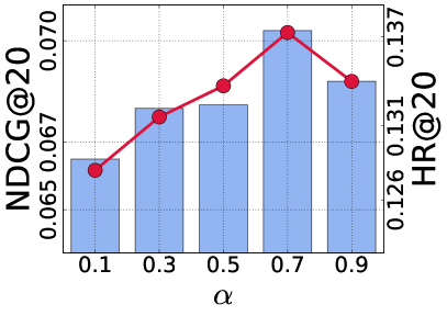
(a) Beauty

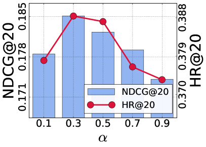
(b) ML-1M

Figure 5: Sensitivity to $\alpha$. More results in other datasets are in Appendix.

(a) Beauty

(b) ML-1M

Figure 6: Sensitivity to $c$. More results in other datasets are in Appendix.

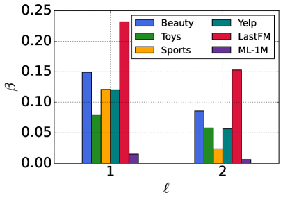
(a) Visualization of learned $\bm{\beta}$

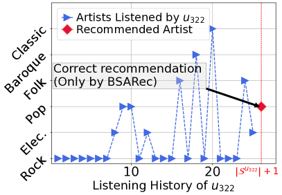
(b) Case study

Figure 7: (a) Visualization of learned $\bm{\beta}$, and (b) an example recommendation in LastFM. The y-axis represents the genre of the artist the user listened to.

Case Study

We introduce case study obtained from our experiment. In Fig. 7 (b), we analyze one of the heavy users in LastFM. The user $u_{322}$ constantly listens to artists, mainly in the rock genre. In other models, $u_{322}$ cannot capture sudden interaction changes in the next step. Only BSARec recommends an artist from the pop genre as the next artist $u_{322}$ will listen to. This shows that BSARec can capture high-frequency signals that are abrupt changes in user preference.

5.4 Model Complexity and Runtime Analyses

To evaluate the overhead of BSARec, we evaluate the number of parameters and runtime per epoch during training. The results are shown in Table 4. Overall, BSARec increases total parameters marginally. BSARec is actually faster to train than FEARec and DuoRec using contastive learning. For ML-1M, BSARec is 7.02% slower than SASRec, but considering the performance difference, it is a big deal.

Methods		Beauty			ML-1M
		# params	s/epoch		# params	s/epoch
BSARec		878,208	12.75		322,368	20.73
SASRec		877,824	10.41		321,984	19.37
DuoRec		877,824	19.26		321,984	32.33
FEARec		877,824	156.83		321,984	278.24

Table 4: The number of parameters and training time (runtime per epoch) on Beauty and ML-1M. More results in other datasets are in Appendix.

6 Related Work

6.1 Sequential Recommendation

In the domain of SR, the primary objective is to recommend the next item based on the sequential patterns inherent in the user’s historical interactions. FPMC (Rendle, Freudenthaler, and Schmidt-Thieme 2010) in SR incorporates Markov Chains to capture item-item transitions. Fossil (He and McAuley 2016) extends the approach to consider higher-order item transitions, improving its predictive capabilities.

Several notable works have been conducted in this area, each presenting distinct approaches. Early approaches (Rendle, Freudenthaler, and Schmidt-Thieme 2010; He and McAuley 2016) tried to improve prediction by utilizing Markov Chains to transition between items in the SR. Another avenue of SR leverages convolutional neural networks for sequence modeling, as seen in Caser (Tang and Wang 2018). Caser treats the embedding matrix of items in the sequence as an image and applies convolution operators to capture local item-item interactions effectively.

The advancements in deep neural network-based SR methods have also made a profound impact on SR, leading to the adoption of RNNs and the self-attention mechanisms. For instance, GRU4Rec (Hidasi et al. 2016) proposes the utilization of GRUs. The success of Transformer-based models, exemplified by Transformer, has further motivated researchers to explore the potential of self-attention in SR. Notably, SASRec (Kang and McAuley 2018) and BERT4Rec (Sun et al. 2019) have demonstrated the efficacy of self-attention. These works signify the continued pursuit of enhanced SR methods by integrating self-attention.

With their success, sequential recommendations are actively studied (Qiu et al. 2022; Zhou et al. 2022; Du et al. 2023; Lin et al. 2023; Zhou et al. 2023; Yue et al. 2023; Liu et al. 2023; Jiang et al. 2023). Recently, contrastive learning has been used as an aid to improve SR performance. DuoRec (Qiu et al. 2022) uses unsupervised model-level augmentation and supervised semantic positive samples for contrastive learning. FMLPRec (Zhou et al. 2022) proposes a filter-enhanced MLP. This approach utilizes a global filter to eliminate frequency domain noise. However, the global filter tends to assign more significance to lower frequencies while undervaluing relatively higher frequencies. FEARec (Du et al. 2023) is a contrastive learning-based model that uses time domain attention and autocorrelation. AdaMCT (Jiang et al. 2023), which appears at the same time as our work, incorporates locality-induced bias into the Transformer using a local convolutional filter.

6.2 Oversmoothing and Transformers

The concept of oversmoothing was first presented by Li, Han, and Wu (2018) in the field of graph research. Intuitively, the expression converges to a constant after repeatedly exchanging messages with neighbors as the layer of graph neural networks goes to infinity, and research is active to solve this problem (Rusch et al. 2022; Choi et al. 2023b). Coincidentally, a parallel occurrence to oversmoothing is observed in Transformers. Early work empirically attributes this to attention collapse or patch or token uniformity (Zhou et al. 2021; Gong et al. 2021). Dong, Cordonnier, and Loukas (2021) also reveals that the pure Transformer output converges to a rank 1 matrix. There have been several attempts in computer vision to solve this problem (Wang et al. 2022; Guo et al. 2023; Choi et al. 2023c), but in SR, there is only one study that solves fast singular value decay (Fan et al. 2023).

7 Conclusion

This paper delves into the realm of sequential recommendation (SR) built upon Transformers, an avenue that has garnered substantial success and popularity. The self-attention within Transformers encounters limitations stemming from insufficient inductive bias and its low-pass filtering properties. We also reveal the oversmoothing due to this low-pass filter in SR. To address this, we introduce BSARec, which uses a combination of attentive inductive bias and vanilla self-attention and integrates low and high-frequencies to mitigate oversmoothing. By understanding and addressing the limitations of self-attention, BSARec significantly advances SR. Our model surpasses 7 baseline methods across 6 datasets in recommendation performance. In future work, we aim to delve deeper into the frequency dynamics of the self-attention for SR.

Appendix A More Preliminaries on Fourier Transform

We provide the detailed background of Fourier transform. Here, we only consider discrete Fourier transform (DFT) on real-value domain $\mathcal{F}:\mathbb{R}^{N}\rightarrow\mathbb{C}^{N}$. DFT is a transformation used to convert a discrete time-domain signal into a discrete frequency-domain representation. This transformation is particularly useful in signal processing and many other fields. In this paper, we use the following expression of the Fourier basis, which is the row of this matrix: $\bm{f}_{j}=[e^{2\pi i(j-1)\cdot 0}\ldots e^{2\pi i(j-1)(N-1)}]^{\mathtt{T}}/\sqrt{N}\in\mathbb{R}^{N}$, where $i$ is the imaginary unit and $j$ denotes the $j$-th row. The DFT is often used in its matrix form as a transformation matrix, which can be applied to a signal through matrix multiplication. We can define the DFT matrix as follows:

$$\mathbf{F}=\frac{1}{\sqrt{N}}\begin{bmatrix}1&1&\ldots&1\\ 1&e^{2\pi i}&\ldots&e^{2\pi i(N-1)}\\ \vdots&\vdots&\ddots&\vdots\\ 1&e^{2\pi i(j-1)\cdot 1}&\ldots&e^{2\pi i(j-1)\cdot(N-1)}\\ \vdots&\vdots&\ddots&\vdots\\ 1&e^{2\pi i(N-1)}&\ldots&e^{2\pi i(N-1)^{2}}\end{bmatrix},$$ (12)

and its inverse Fourier transform is DFT. Specifically, when the matrix representation of the IDFT is the conjugate transpose (Hermitian) of the DFT matrix, scaled by a factor of $1/\sqrt{N}$, the transformation becomes unitary. The IDFT matrix can be expressed as:

$$\mathbf{F}^{-1}=\frac{1}{\sqrt{N}}\mathbf{F}^{H},$$ (13)

where $\mathbf{F}^{H}$ denotes the conjugate transpose of $\mathbf{F}$. The factor $1/\sqrt{N}$ ensures that the transformation is norm-preserving, meaning that the energy of the signal remains invariant under both the DFT and IDFT. This normalization underpins the unitary nature of the transformation and emphasizes the duality between the time and frequency domains in discrete signal processing.

This relationship emphasizes that the IDFT is not an isolated operation, but rather intimately linked with the DFT through the conjugate transpose operation and a normalization factor. By utilizing the DFT matrix $\mathbf{F}$ in this manner, we are able to conduct the IDFT without resorting to a separate transformation matrix.

Appendix B Definition of a Low-Pass Filter

In this paper, a specific type of filter that preserves only the low-frequency components while reducing the remaining high-frequency components is called a low-pass filter. More precisely, we define a low-pass filter.

Definition B.1.

Given a transformation $f:\mathbb{R}^{N}\rightarrow\mathbb{R}^{N}$, with indicating the application of $f$ for $t$ times, the $f$ is a low-pass filter if and only if, for all $\bm{x}\in\mathbb{R}^{N}$:

$$\lim_{t\rightarrow\infty}\frac{||HFC(f^{t}(\bm{x}))||_{2}}{||LFC(f^{t}(\bm{x}))||_{2}}=0.$$ (14)

Definition B.1 provides a criterion to evaluate the frequency behavior of a transformation. In essence, if after recurrently applying the transformation $f$ to a $\bm{x}$, and then taking its DFT, the high-frequency components are diminished compared to the low-frequency components as time advances, then $f$ can be described as exhibiting a low-pass behavior.

Appendix C Proof of Theorem 3.1

Theorem 3.1.

Let $\mathbf{A}=\textrm{softmax}(\mathbf{Q}\mathbf{K}^{\mathtt{T}}/\sqrt{d})$. Then $\mathbf{A}$ inherently acts as a low-pass filter. For all $\bm{x}\in\mathbb{R}^{N}$, in other words,

$$\lim_{t\rightarrow\infty}\frac{||HFC(f^{t}(\bm{x}))||_{2}}{||LFC(f^{t}(\bm{x}))||_{2}}=0.$$ (15)

Proof.

Given the matrix $\mathbf{A}$ defined by the softmax function, it has non-negative entries, and the sum of each row is unity. We aim to describe the evolution of the $\bm{x}$ under repeated application of $\mathbf{A}$.

Let’s denote the Jordan Canonical Form of $\mathbf{A}$ as $\mathbf{J}$, with the similarity transformation represented by the matrix $\mathbf{P}$, such that:

$$\mathbf{A}=\mathbf{P}\mathbf{J}\mathbf{P}^{-1},$$ (16)

where $\mathbf{J}$ is block-diagonal, with each block corresponding to an eigenvalue and its associated Jordan chains. The largest eigenvalue, by the Perron-Frobenius theorem, is real, non-negative, and dominant. Let’s denote this eigenvalue by $\lambda_{1}$.

Now, consider the repeated application of $\mathbf{A}$:

$$f^{t}(\bm{x})=\mathbf{A}^{t}\bm{x}=(\mathbf{P}\mathbf{J}\mathbf{P}^{-1})^{t}\bm{x}.$$ (17)

Expanding using the binomial theorem and taking into account the structure of the Jordan blocks, we can see that the dominant behavior for large $t$ will be $\lambda^{t}_{1}$. Other terms involving smaller eigenvalues or higher powers of $t$ in the Jordan blocks will become negligible over time, compared to the term with $\lambda^{t}_{1}$.

Expressing the transformation in the frequency domain, high-frequency components attenuate faster than the primary low-frequency component. This is due to the term $\lambda^{t}_{1}$ becoming overwhelmingly dominant as $t$ grows, causing other components to diminish in comparison.

Thus, in the context of our filter definitions, it becomes evident that:

$$\lim_{t\rightarrow\infty}\frac{||HFC[f^{t}(\bm{x})-\lambda^{t}_{1}\mathbf{v}_{1}]||_{2}}{||LFC[\lambda^{t}_{1}\mathbf{v}_{1}]||_{2}}=0$$ (18)

Here, $\mathbf{v}_{1}$ is the generalized eigenvector corresponding to $\lambda_{1}$.

This behavior is emblematic of a low-pass filter, reaffirming the low-pass nature of $\mathbf{A}$. Importantly, this is irrespective of the specific configurations of the input matrices $\mathbf{Q}$ and $\mathbf{K}$. ∎

Appendix D Additional Details for Experiments

D.1 Details of Datasets

We provide 6 benchmark datasets used for our experiments. Table 5 summarizes the statistical information of the processed datasets.

	# Users	# Items	# Interactions	Avg. Length	Sparsity
Beauty	22,363	12,101	198,502	8.9	99.93%
Sports	25,598	18,357	296,337	8.3	99.95%
Toys	19,412	11,924	167,597	8.6	99.93%
Yelp	30,431	20,033	316,354	10.4	99.95%
LastFM	1,090	3,646	52,551	48.2	98.68%
ML-1M	6,041	3,417	999,611	165.5	95.16%

Table 5: Statistics of the processed datasets

• Amazon Beauty, Sports, Toys are three sub-categories of Amazon dataset (McAuley et al. 2015) which contains series of product reviews crawled from the Amazon.com. These datasets are known for its high sparsity and short sequence lengths, and widely used for SR.

• Yelp is a popular business recommendation dataset. We only treat the transaction records after January 1st, 2019 since it is very large.

• ML-1M (Harper and Konstan 2015) is the popular movie recommendation dataset provided by MovieLens. It has the longest average interaction length among our datasets.

• LastFM contains user interaction with music, such as artist listening records. It is used to recommend musicians to users in SR with long sequence lengths.

D.2 Details of Baselines

We compare our method with well-known SR baselines with 3 categories. The detailed information of baselines are follows:

• RNN or CNN-based sequential models: GRU4Rec (Hidasi et al. 2016) is a model that incorporate GRU for SR. Caser (Tang and Wang 2018) is a CNN-based method capturing high-order patterns by applying horizontal and vertical convolutional operations for SR.

• Transformer-based sequential models: SASRec (Kang and McAuley 2018) is the first sequential recommender based on the self-attention. It is a popular baseline in SR. BERT4Rec (Sun et al. 2019) uses a masked item training scheme similar to the masked language model sequential in NLP. The backbone is the bi-directional self-attention mechanism. FMLPRec (Zhou et al. 2022) is an all-MLP model with learnable filters for SR.

• Transformer-based sequential models with contrsastive learning: DuoRec (Qiu et al. 2022) uses unsupervised model-level augmentation and supervised semantic positive samples for contrastive learning. FEARec (Du et al. 2023) is a SR model based on contrastive learning using time domain attention and autocorrelation.

D.3 Experimental Settings & Hyperparameters

The following software and hardware environments were used for all experiments: Ubuntu 18.04 LTS, Python 3.9.7, PyTorch 1.8.1, Numpy 1.24.3, Scipy 1.11.1, CUDA 11.1, and NVIDIA Driver 465.19, and i9 CPU, and NVIDIA RTX 3090.

For reproducibility, we introduce the best hyperparameter configurations for each dataset in Table 6. We conducted experiments under the following hyperparameters: the $\alpha$ is in $\{0.1,0.3,0.5,0.7,0.9\}$, $c$ is in $\{1,3,5,7,9\}$, and the number of heads in Transformer $h$ is chosen from $\{1,2,4\}$. For training, the Adam optimizer is optimized with learning rate in {$5\text{\times}{10}^{-4}$, $1\text{\times}{10}^{-3}$}.

	Beauty	Sports	Toys	Yelp	LastFM	ML-1M
$\alpha$	0.7	0.3	0.7	0.7	0.9	0.3
$c$	5	5	3	3	3	9
$h$	1	4	1	4	1	4
lr	$5\text{\times}{10}^{-4}$	$1\text{\times}{10}^{-3}$	$1\text{\times}{10}^{-3}$	$1\text{\times}{10}^{-3}$	$1\text{\times}{10}^{-3}$	$5\text{\times}{10}^{-4}$

Table 6: Best hyperparameters of BSARec on all datasets

Appendix E Ablation Studies

Table 7 shows the results of the ablation study on all datasets. For all datasets, BSARec, which utilizes $\mathbf{A}$ and $\mathbf{A}_{\textrm{IB}}$, outperforms “Only $\mathbf{A}$” and “Only $\mathbf{A}_{\textrm{IB}}$”. This results show that both are required to achieve the best accuracy. We also conduct an ablation study on $\bm{\beta}$. We check the effect of the learnable vector $\bm{\beta}$ and the learnable scalar parameter $\beta$. Rescaling high frequencies by the learnable vector $\beta$ has better recommendation performance than using the scalar $\beta$.

Methods		Beauty			Sports			Toys			Yelp			LastFM			ML-1M
		HR@20	NDCG@20		HR@20	NDCG@20		HR@20	NDCG@20		HR@20	NDCG@20		HR@20	NDCG@20		HR@20	NDCG@20
BSARec		0.1373	0.0703		0.0858	0.0422		0.1435	0.0768		0.0746	0.0302		0.1174	0.0526		0.3884	0.1851
Only $\mathbf{A}$		0.1265	0.0657		0.0779	0.0382		0.1320	0.0720		0.0618	0.0248		0.0899	0.0430		0.3826	0.1846
Only $\mathbf{A}_{\textrm{IB}}$		0.1338	0.0677		0.0857	0.0416		0.1402	0.0744		0.0705	0.0287		0.1009	0.0455		0.3780	0.1807
Scalar $\beta$		0.1333	0.0685		0.0838	0.0405		0.1435	0.0756		0.0707	0.0291		0.1092	0.0497		0.3762	0.1794

Table 7: Ablation on all datasets

Appendix F Sensitivity Analyses

Fig. 8 shows the HR@20 and NDCG@20 by varying the $\alpha$ on all datasets. For Beauty, Toys, Yelp and LastFM, a larger value of $\alpha$ is preferred. For Sports and ML-1M, the best accuracy is achieve when $\alpha$. The balance between the self-attention matrix and the inductive bias varies across datasets to these results.

Fig. 9 shows the HR@20 and NDCG@20 by varying the $c$ on all datasets. For Beauty and Sports, the best accuracy is achieve when $c$ is 5. For Toys, Yelp and LastFM, with $c$ = 3, we can achieve the best accuracy. For ML-1M, a larger value of $c$ is preferred. The number of lowest frequency components varies across datasets according to these results.

(a) Beauty

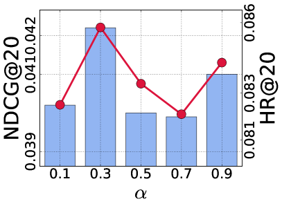
(b) Sports

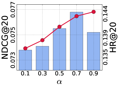
(c) Toys

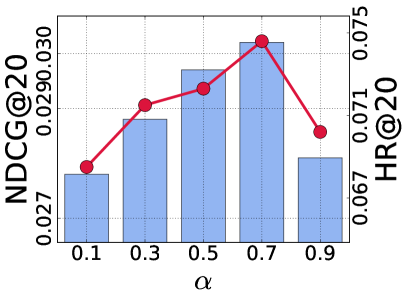
(d) Yelp

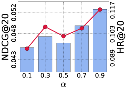
(e) LastFM

(f) ML-1M

Figure 8: Sensitivity to $\alpha$ on all datasets

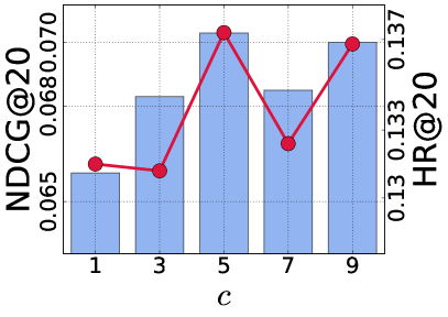
(a) Beauty

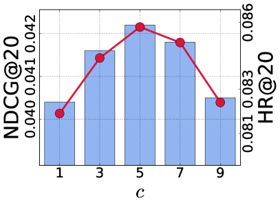
(b) Sports

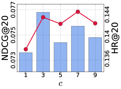
(c) Toys

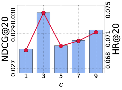
(d) Yelp

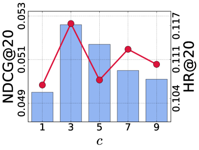
(e) LastFM

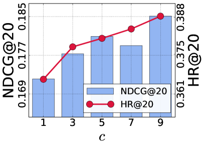
(f) ML-1M

Figure 9: Sensitivity to $c$ on all datasets

Appendix G Model Complexity and Runtime Analyses

To evaluate the complexity and efficiency of BSARec, we evaluate the number of parameters and runtime per epoch. Results for all datasets are shown in Table 8. Overall, BSARec slightly increases the total parameters. However, if we use $\bm{\beta}$ as one scalar parameter $\beta$ in our model, the number of parameters may not make much difference. It only increases by 258 parameters compared to SASRec, DuoRec and FEARec. We show that BSARec has faster runtime times per epoch than FEARec and DuoRec across all datasets.

Methods		Beauty			Sports			Toys			Yelp			LastFM			ML-1M
		# params	s/epoch		# params	s/epoch		# params	s/epoch		# params	s/epoch		# params	s/epoch		# params	s/epoch
BSARec		878,208	12.75		1,278,592	18.58		866,880	11.63		1,385,856	21.20		337,088	3.11		322,368	20.73
SASRec		877,824	10.41		1,278,208	15.32		866,496	9.96		1,385,472	18.25		336,704	2.80		321,984	19.37
DuoRec		877,824	19.26		1,278,208	27.99		866,496	18.79		1,385,472	31.08		336,704	4.24		321,984	32.33
FEARec		877,824	156.83		1,278,208	233.42		866,496	132.43		1,385,472	257.56		336,704	27.82		321,984	278.24

Table 8: The number of parameters and training time (runtime per epoch) on all datasets

Appendix H Performance under Different Setting

In our main text, we use the evaluation strategy of DuoRec and FEARec, which employ all the items in the dataset. To further verify the effectiveness of our BSARec, we also conduct experiments under another strategy that SASRec and FMLP-Rec used. For evaluation, SASRec and FMLPRec pair the ground-truth item with 99 randomly sampled negative items that the user has not interacted with.

We select Transformer-based SASRec as the representative baseline model and FMLP-Rec as one of the SOTA baselines. Table 9 shows the results on Beauty, Sports, Toys, Yelp, LastFM, and ML-1M datasets. From the table, we can see similar tendencies as in Table 2. BSARec performs much better than the other two methods. In most of the cases, BSARec outperforms SASRec and FMLP-Rec. These findings indicate that our beyond self-attention layer and attentive inductive bias with frequency rescaler are exactly effective for the SR task.

Dataset	Metric	SASRec	FMLPRec	BSARec
Beauty	HR@5	0.3512	0.3922	0.4312
	HR@10	0.4434	0.4914	0.5225
	NDCG@5	0.2628	0.2964	0.3379
	NDCG@10	0.2926	0.3284	0.3673
	MRR	0.2637	0.2949	0.3350
Sports	HR@5	0.3480	0.3781	0.4133
	HR@10	0.4717	0.4997	0.5303
	NDCG@5	0.2492	0.2739	0.3102
	NDCG@10	0.2891	0.3131	0.3479
	MRR	0.2520	0.2742	0.3089
Toys	HR@5	0.3594	0.3867	0.4224
	HR@10	0.4566	0.4852	0.5180
	NDCG@5	0.2726	0.2926	0.3351
	NDCG@10	0.3040	0.3244	0.3659
	MRR	0.2746	0.2917	0.3349
Yelp	HR@5	0.5553	0.6058	0.6447
	HR@10	0.7406	0.7707	0.7848
	NDCG@5	0.3902	0.4337	0.4824
	NDCG@10	0.4504	0.4873	0.5280
	MRR	0.3748	0.4114	0.4587
LastFM	HR@5	0.2716	0.2853	0.3752
	HR@10	0.3972	0.4138	0.5028
	NDCG@5	0.1871	0.1975	0.2634
	NDCG@10	0.2276	0.2394	0.3045
	MRR	0.1976	0.2081	0.2636
ML-1M	HR@5	0.6874	0.6763	0.7023
	HR@10	0.7904	0.7858	0.7978
	NDCG@5	0.5308	0.5212	0.5646
	NDCG@10	0.5642	0.5568	0.5955
	MRR	0.5020	0.4941	0.5406

Table 9: Performance comparison on 99 negative sampling

References

- Chen et al. (2019) Chen, Q.; Zhao, H.; Li, W.; Huang, P.; and Ou, W. 2019. Behavior sequence transformer for e-commerce recommendation in alibaba. In Proceedings of the 1st International Workshop on Deep Learning Practice for High-dimensional Sparse Data, 1–4.
- Choi et al. (2023a) Choi, J.; Hong, S.; Park, N.; and Cho, S.-B. 2023a. Blurring-Sharpening Process Models for Collaborative Filtering. In SIGIR.
- Choi et al. (2023b) Choi, J.; Hong, S.; Park, N.; and Cho, S.-B. 2023b. GREAD: Graph Neural Reaction-Diffusion Networks. In ICML.
- Choi, Jeon, and Park (2021) Choi, J.; Jeon, J.; and Park, N. 2021. LT-OCF: Learnable-Time ODE-based Collaborative Filtering. In CIKM.
- Choi et al. (2023c) Choi, J.; Wi, H.; Kim, J.; Shin, Y.; Lee, K.; Trask, N.; and Park, N. 2023c. Graph Convolutions Enrich the Self-Attention in Transformers! arXiv preprint arXiv:2312.04234.
- Dong, Cordonnier, and Loukas (2021) Dong, Y.; Cordonnier, J.-B.; and Loukas, A. 2021. Attention is not all you need: Pure attention loses rank doubly exponentially with depth. In ICML, 2793–2803. PMLR.
- Dosovitskiy et al. (2020) Dosovitskiy, A.; Beyer, L.; Kolesnikov, A.; Weissenborn, D.; Zhai, X.; Unterthiner, T.; Dehghani, M.; Minderer, M.; Heigold, G.; Gelly, S.; et al. 2020. An image is worth 16x16 words: Transformers for image recognition at scale. ICLR.
- Du et al. (2023) Du, X.; Yuan, H.; Zhao, P.; Qu, J.; Zhuang, F.; Liu, G.; Liu, Y.; and Sheng, V. S. 2023. Frequency Enhanced Hybrid Attention Network for Sequential Recommendation. In SIGIR, 78–88.
- Fan et al. (2023) Fan, Z.; Liu, Z.; Peng, H.; and Yu, P. S. 2023. Addressing the Rank Degeneration in Sequential Recommendation via Singular Spectrum Smoothing. arXiv preprint arXiv:2306.11986.
- Gao et al. (2023) Gao, C.; Zheng, Y.; Li, N.; Li, Y.; Qin, Y.; Piao, J.; Quan, Y.; Chang, J.; Jin, D.; He, X.; et al. 2023. A survey of graph neural networks for recommender systems: Challenges, methods, and directions. ACM Transactions on Recommender Systems, 1(1): 1–51.
- Gong et al. (2021) Gong, C.; Wang, D.; Li, M.; Chandra, V.; and Liu, Q. 2021. Vision transformers with patch diversification. arXiv preprint arXiv:2104.12753.
- Guo et al. (2023) Guo, X.; Wang, Y.; Du, T.; and Wang, Y. 2023. Contranorm: A contrastive learning perspective on oversmoothing and beyond. In ICLR.
- Hansen et al. (2020) Hansen, C.; Hansen, C.; Maystre, L.; Mehrotra, R.; Brost, B.; Tomasi, F.; and Lalmas, M. 2020. Contextual and sequential user embeddings for large-scale music recommendation. In RecSys, 53–62.
- Harper and Konstan (2015) Harper, F. M.; and Konstan, J. A. 2015. The movielens datasets: History and context. Acm transactions on interactive intelligent systems (tiis), 5(4): 1–19.
- He and McAuley (2016) He, R.; and McAuley, J. 2016. Fusing similarity models with markov chains for sparse sequential recommendation. In ICDM, 191–200. IEEE.
- He et al. (2020) He, X.; Deng, K.; Wang, X.; Li, Y.; Zhang, Y.; and Wang, M. 2020. LightGCN: Simplifying and Powering Graph Convolution Network for Recommendation. In SIGIR.
- He and Wai (2021) He, Y.; and Wai, H.-T. 2021. Identifying first-order lowpass graph signals using perron frobenius theorem. In ICASSP 2021-2021 IEEE International Conference on Acoustics, Speech and Signal Processing (ICASSP), 5285–5289. IEEE.
- Hidasi et al. (2016) Hidasi, B.; Karatzoglou, A.; Baltrunas, L.; and Tikk, D. 2016. Session-based recommendations with recurrent neural networks. In ICLR.
- Hong et al. (2022) Hong, S.; Jo, M.; Kook, S.; Jung, J.; Wi, H.; Park, N.; and Cho, S.-B. 2022. TimeKit: A Time-series Forecasting-based Upgrade Kit for Collaborative Filtering. In 2022 IEEE International Conference on Big Data (Big Data), 565–574. IEEE.
- Huang et al. (2018) Huang, X.; Qian, S.; Fang, Q.; Sang, J.; and Xu, C. 2018. CSAN: Contextual self-attention network for user sequential recommendation. In ACM MM, 447–455.
- Jiang et al. (2023) Jiang, J.; Zhang, P.; Luo, Y.; Li, C.; Kim, J. B.; Zhang, K.; Wang, S.; Xie, X.; and Kim, S. 2023. AdaMCT: adaptive mixture of CNN-transformer for sequential recommendation. In CIKM.
- Jiang et al. (2016) Jiang, S.; Qian, X.; Mei, T.; and Fu, Y. 2016. Personalized travel sequence recommendation on multi-source big social media. IEEE Transactions on Big Data, 2(1): 43–56.
- Kang and McAuley (2018) Kang, W.-C.; and McAuley, J. 2018. Self-attentive sequential recommendation. In ICDM, 197–206. IEEE.
- Kong et al. (2022) Kong, T.; Kim, T.; Jeon, J.; Choi, J.; Lee, Y.-C.; Park, N.; and Kim, S.-W. 2022. Linear, or Non-Linear, That is the Question! In WSDM, 517–525.
- Krichene and Rendle (2020) Krichene, W.; and Rendle, S. 2020. On sampled metrics for item recommendation. In Proceedings of the 26th ACM SIGKDD international conference on knowledge discovery & data mining, 1748–1757.
- Li, Wang, and McAuley (2020) Li, J.; Wang, Y.; and McAuley, J. 2020. Time interval aware self-attention for sequential recommendation. In WSDM, 322–330.
- Li, Han, and Wu (2018) Li, Q.; Han, Z.; and Wu, X.-M. 2018. Deeper insights into graph convolutional networks for semi-supervised learning. In AAAI.
- Lin et al. (2023) Lin, G.; Gao, C.; Zheng, Y.; Chang, J.; Niu, Y.; Song, Y.; Gai, K.; Li, Z.; Jin, D.; Li, Y.; et al. 2023. Mixed Attention Network for Cross-domain Sequential Recommendation. arXiv preprint arXiv:2311.08272.
- Liu et al. (2023) Liu, Q.; Yan, F.; Zhao, X.; Du, Z.; Guo, H.; Tang, R.; and Tian, F. 2023. Diffusion Augmentation for Sequential Recommendation. In CIKM, 1576–1586.
- McAuley et al. (2015) McAuley, J.; Targett, C.; Shi, Q.; and Van Den Hengel, A. 2015. Image-based recommendations on styles and substitutes. In Proceedings of the 38th international ACM SIGIR conference on research and development in information retrieval, 43–52.
- Meyer and Stewart (2023) Meyer, C. D.; and Stewart, I. 2023. Matrix analysis and applied linear algebra. SIAM.
- Qiu et al. (2022) Qiu, R.; Huang, Z.; Yin, H.; and Wang, Z. 2022. Contrastive learning for representation degeneration problem in sequential recommendation. In WSDM, 813–823.
- Rendle, Freudenthaler, and Schmidt-Thieme (2010) Rendle, S.; Freudenthaler, C.; and Schmidt-Thieme, L. 2010. Factorizing personalized markov chains for next-basket recommendation. In TheWebConf (former WWW), 811–820.
- Rusch et al. (2022) Rusch, T. K.; Chamberlain, B.; Rowbottom, J.; Mishra, S.; and Bronstein, M. 2022. Graph-Coupled Oscillator Networks. In ICML, volume 162, 18888–18909.
- Sandryhaila and Moura (2014) Sandryhaila, A.; and Moura, J. M. 2014. Discrete signal processing on graphs: Frequency analysis. IEEE Transactions on Signal Processing, 62(12): 3042–3054.
- Schedl et al. (2018) Schedl, M.; Zamani, H.; Chen, C.-W.; Deldjoo, Y.; and Elahi, M. 2018. Current challenges and visions in music recommender systems research. International Journal of Multimedia Information Retrieval, 7: 95–116.
- Sun et al. (2019) Sun, F.; Liu, J.; Wu, J.; Pei, C.; Lin, X.; Ou, W.; and Jiang, P. 2019. BERT4Rec: Sequential recommendation with bidirectional encoder representations from transformer. In CIKM, 1441–1450.
- Tang and Wang (2018) Tang, J.; and Wang, K. 2018. Personalized top-n sequential recommendation via convolutional sequence embedding. In WSDM, 565–573.
- Vaswani et al. (2017) Vaswani, A.; Shazeer, N.; Parmar, N.; Uszkoreit, J.; Jones, L.; Gomez, A. N.; Kaiser, Ł.; and Polosukhin, I. 2017. Attention is all you need. In NeurIPS.
- Wang et al. (2022) Wang, P.; Zheng, W.; Chen, T.; and Wang, Z. 2022. Anti-Oversmoothing in Deep Vision Transformers via the Fourier Domain Analysis: From Theory to Practice. In ICLR.
- Wu, Cai, and Wang (2020) Wu, J.; Cai, R.; and Wang, H. 2020. Déjà vu: A contextualized temporal attention mechanism for sequential recommendation. In TheWebConf (former WWW), 2199–2209.
- Wu et al. (2020) Wu, L.; Li, S.; Hsieh, C.-J.; and Sharpnack, J. 2020. SSE-PT: Sequential recommendation via personalized transformer. In RecSys, 328–337.
- Wu et al. (2022) Wu, S.; Sun, F.; Zhang, W.; Xie, X.; and Cui, B. 2022. Graph neural networks in recommender systems: a survey. ACM Computing Surveys, 55(5): 1–37.
- Yue et al. (2023) Yue, Z.; Wang, Y.; He, Z.; Zeng, H.; McAuley, J.; and Wang, D. 2023. Linear Recurrent Units for Sequential Recommendation. arXiv preprint arXiv:2310.02367.
- Zhang et al. (2019) Zhang, T.; Zhao, P.; Liu, Y.; Sheng, V. S.; Xu, J.; Wang, D.; Liu, G.; Zhou, X.; et al. 2019. Feature-level Deeper Self-Attention Network for Sequential Recommendation. In IJCAI, 4320–4326.
- Zhou et al. (2021) Zhou, D.; Kang, B.; Jin, X.; Yang, L.; Lian, X.; Jiang, Z.; Hou, Q.; and Feng, J. 2021. Deepvit: Towards deeper vision transformer. arXiv preprint arXiv:2103.11886.
- Zhou et al. (2020) Zhou, K.; Wang, H.; Zhao, W. X.; Zhu, Y.; Wang, S.; Zhang, F.; Wang, Z.; and Wen, J.-R. 2020. S3-rec: Self-supervised learning for sequential recommendation with mutual information maximization. In CIKM, 1893–1902.
- Zhou et al. (2022) Zhou, K.; Yu, H.; Zhao, W. X.; and Wen, J.-R. 2022. Filter-enhanced MLP is all you need for sequential recommendation. In TheWebConf (former WWW), 2388–2399.
- Zhou et al. (2023) Zhou, P.; Ye, Q.; Xie, Y.; Gao, J.; Wang, S.; Kim, J. B.; You, C.; and Kim, S. 2023. Attention Calibration for Transformer-based Sequential Recommendation. In CIKM, 3595–3605.