Image Restoration Through Generalized Ornstein-Uhlenbeck Bridge

Abstract

Diffusion models possess powerful generative capabilities enabling the mapping of noise to data using reverse stochastic differential equations. However, in image restoration tasks, the focus is on the mapping relationship from low-quality images to high-quality images. To address this, we introduced the Generalized Ornstein-Uhlenbeck Bridge (GOUB) model. By leveraging the natural mean-reverting property of the generalized OU process and further adjusting the variance of its steady-state distribution through the Doob’s h–transform, we achieve diffusion mappings from point to point with minimal cost. This allows for end-to-end training, enabling the recovery of high-quality images from low-quality ones. Additionally, we uncovered the mathematical essence of some bridge models, all of which are special cases of the GOUB and empirically demonstrated the optimality of our proposed models. Furthermore, benefiting from our distinctive parameterization mechanism, we proposed the Mean-ODE model that is better at capturing pixel-level information and structural perceptions. Experimental results show that both models achieved state-of-the-art results in various tasks, including inpainting, deraining, and super-resolution. Code is available at https://github.com/Hammour-steak/GOUB.

1 Introduction

Image restoration is the process of transforming low-quality images into their high-quality counterparts in the field of computer vision, boasts a long and rich history (Banham and Katsaggelos, 1997; Zhou et al., 1988; Liang et al., 2021; Luo et al., 2023a). It encompasses a suite of classical tasks, including deraining (Zhang and Patel, 2017; Yang et al., 2020; Xiao et al., 2022), denoising (Zhang et al., 2018a; Li et al., 2022; Soh and Cho, 2022; Zhang et al., 2023a), deblurring (Yuan et al., 2007; Kong et al., 2023), inpainting (Jain et al., 2023; Zhang et al., 2023b), and super-resolution (Dong et al., 2015; Zamfir et al., 2023), among others. Owing to the diminution of critical information during the degradation from high-quality to low-quality images, image restoration is also characterized as an ill-posed inverse problem: it is not feasible to losslessly reconstruct high-dimensional information from low-dimensional data.

In recent years, diffusion models (Sohl-Dickstein et al., 2015; Ho et al., 2020; Song and Ermon, 2019; Song et al., 2020; Karras et al., 2022) have garnered significant attention for their remarkable performance in generative tasks. Essentially, they utilize neural networks to learn the reverse-time Stochastic Differential Equation (SDE) (Anderson, 1982) corresponding to a given forward SDE. More precisely, they are oriented towards learning the scores (Song et al., 2020), i.e., the gradients of the logarithm of probability densities.

Consequently, leveraging the significant advantages of diffusion models in generative tasks, several studies have applied them to image restoration and have achieved favorable results. A majority of these studies utilize the concept of conditional diffusion models, including classifier-guidance (Dhariwal and Nichol, 2021) or classifier-free (Ho and Salimans, 2022) approaches, by taking low-quality images as conditions (Kawar et al., 2021; Saharia et al., 2022; Kawar et al., 2022; Chung et al., 2022a, b; Wang et al., 2023). This strategy effectively guides the generation process, thus facilitating the restoration of high-quality images. Nevertheless, these approaches require the integration of substantial prior knowledge specific to each task such as degradation matrices, limiting their universality.

Additionally, some studies have attempted to establish a point-to-point mapping from low-quality to high-quality images, thereby learning the general degradation and restoration process of images and circumventing the need for modeling specific tasks. In the terms of diffusion models, such a mapping can be actualized through the ’bridge’—a stochastic process with fixed starting and ending points. However, some bridge models face challenges in learning likelihoods (Liu et al., 2022a), necessitating reliance on cumbersome iterative approximation methods (De Bortoli et al., 2021; Su et al., 2022; Shi et al., 2023), which pose significant constraints in practical applications; others do not take into account the optimal diffusion approach (Liu et al., 2023; Li et al., 2023; Zhou et al., 2023), thus introducing unnecessary costs and limiting the performance of the model.

To address the aforementioned issues, we leverage the natural mean-reverting characteristic of the Generalized Ornstein-Uhlenbeck (GOU) process and propose an image restoration bridge model—GOUB (Generalized Ornstein-Uhlenbeck Bridge), based on the GOU process Doob’s h-transform. The overview of the proposed image restoration GOUB can be seen in Figure 1. The forward process of the model initiates a point-to-point diffusion from high-quality images to their corresponding low-quality counterparts, readily facilitates the learning of its reverse process through maximum likelihood estimation. Therefore, it is able to restore low-quality images to corresponding high-quality images, without being limited by a specific task. Our main contributions can be summarized as follows:

• We introduce a novel image restoration model GOUB, which connects the degradation and restoration of high and low-quality images through a diffusion process. This process can be approximated by neural networks and optimized efficiently via maximum likelihood estimation.

• Benefiting from the distinctive features of parameterization mechanism, we introduced Mean-ODE model, which demonstrates a strong ability in capturing both pixel-level information and structural perceptions.

• We uncovered the mathematical essence of some bridge models, all of which are special cases of the GOUB and empirically demonstrated the optimality of our proposed models.

• Our model has achieved state-of-the-art results on numerous image restoration tasks, such as inpainting, deraining, denoising and dehazing, among others.

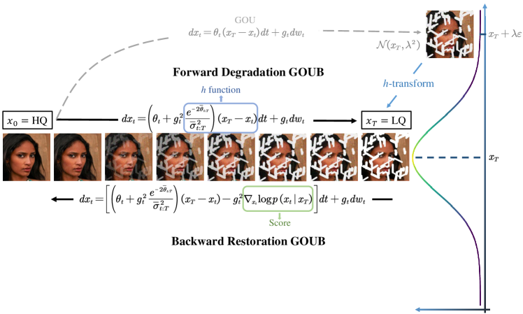
Figure 1: The overview of the proposed image restoration GOUB. It can be observed that the GOU process is capable of transferring High Quality (HQ) into noisy Low Quality (LQ). Additionally, through the application of h-transform, minor adjustments can be made to the entire process, enabling the GOUB model to precisely bridge the gap between HQ and LQ.

2 Preliminaries

2.1 Score-based Diffusion Model

The score-based diffusion model(Sohl-Dickstein et al., 2015; Ho et al., 2020; Song et al., 2020) is a category of generative model that seamlessly transitions data into noise via a diffusion process and generates samples by learning and adapting the reverse process(Anderson, 1982). Let $p(\mathbf{x_{0}})$ denote the unknown distribution of a dataset consisting of $n$-dimensional i.i.d. samples. The time-dependent forward process of the diffusion model can be described by the following SDE:

$$\mathrm{d}\mathbf{x}_{t}=\mathbf{f}\left(\mathbf{x}_{t},t\right)\mathrm{d}t+g_{t}\mathrm{d}\mathbf{w}_{t},\qquad\mathbf{x}_{0}\sim p\left(\mathbf{x}_{0}\right),$$ (1)

where $\mathbf{f}:\mathbb{R}^{n}\rightarrow\mathbb{R}^{n}$ is the drift coefficient, $g_{t}:\mathbb{R}\rightarrow\mathbb{R}$ is the scalar diffusion coefficient and $\mathbf{w}_{t}$ denotes the standard Brownian motion. Typically, $p(\mathbf{x}_{0})$ evolves over time $t$ from 0 to a sufficiently large $T$ into $p(\mathbf{x}_{T})$ through the SDE, such that $p(\mathbf{x}_{T})$ will approximate an tractable prior distribution $p_{\text{prior}}(\mathbf{x})$. Meanwhile, the forward SDE has a corresponding reverse time SDE whose closed form is given by:

$$\mathrm{d}\mathbf{x}_{t}=\left[\mathbf{f}\left(\mathbf{x}_{t},t\right)-g^{2}_{t}\nabla_{\mathbf{x}_{t}}\log p(\mathbf{x}_{t})\right]\mathrm{d}t+g_{t}\mathrm{d}\mathbf{w}_{t},\qquad\mathbf{x}_{T}\sim p\left(\mathbf{x}_{T}\right).$$ (2)

Starting from time $T$, $p(\mathbf{x}_{T})$ can progressively transform to $p(\mathbf{x}_{0})$ by traversing the trajectory of the reverse SDE. Specifically and practically, one can sample $\mathbf{x}_{T}$ from the prior distribution $p(\mathbf{x}_{T})\approx p_{\text{prior}}(\mathbf{x})$ and obtain the sample $\mathbf{x}_{0}$ through the discretized reverse SDE, thereby completing the image generation process. The remaining crucial task is the estimation of the score $\nabla_{\mathbf{x}_{t}}\log p(\mathbf{x}_{t})$ which can typically parameterize as $\mathbf{s}_{\bm{\theta}}(\mathbf{x}_{t},t)$ and employ conditional score matching(Vincent, 2011) as the loss function for training:

$$\mathcal{L} =\frac{1}{2}\int_{0}^{T}{\mathbb{E}_{p\left(\mathbf{x}_{t}\right)}\left[\lambda\left(t\right)\left\|\nabla_{\mathbf{x}_{t}}\log p\left(\mathbf{x}_{t}\right)-\mathbf{s}_{\bm{\theta}}\left(\mathbf{x}_{t},t\right)\right\|\right]\mathrm{d}t}$$ (3)

$$=\frac{1}{2}\int_{0}^{T}{\mathbb{E}_{p\left(\mathbf{x}_{0},\mathbf{x}_{t}\right)}\left[\lambda\left(t\right)\left\|\nabla_{\mathbf{x}_{t}}\log p\left(\mathbf{x}_{t}\mid\mathbf{x}_{0}\right)-\mathbf{s}_{\bm{\theta}}\left(\mathbf{x}_{t},t\right)\right\|\right]\mathrm{d}t}+C,$$

where $\lambda(t)$ serves as a weighting function. The study(Song et al., 2021) mentions that selecting $g^{2}_{t}$ yields a more optimal upper bound on the negative log-likelihood. The second line of the aforementioned formula is actually the most commonly used, as the conditional probability $p(\mathbf{x}_{t}\mid\mathbf{x}_{0})$ is generally accessible. Ultimately, utilizing the trained score $\mathbf{s}_{\bm{\theta}}(\mathbf{x}_{t},t)$, samples can be generated through the numerical solution (Euler–Maruyama, Runge-Kutta, Heun, etc.) of Equation (2) via iterative steps.

2.2 Generalized Ornstein-Uhlenbeck process

The generalized Ornstein-Uhlenbeck process is the time-varying OU process (Ahmad, 1988). It is a stationary Gaussian-Markov process, whose marginal distribution gradually tends towards a stable mean over time and exhibits mean-reverting characteristics, and is generally defined as follows:

$$\mathrm{d}\mathbf{x}_{t}=\theta_{t}\left(\bm{\mu}-\mathbf{x}_{t}\right)\mathrm{d}t+g_{t}\mathrm{d}\mathbf{w}_{t},$$ (4)

where $\bm{\mu}$ is a given state vector, $\theta_{t}$ denotes a scalar drift coefficient and $g_{t}$ represents the diffusion coefficient. In general, we are more concerned with the relationship: $2\lambda^{2}=g^{2}_{t}/\theta_{t}$, and can readily select appropriate $\theta_{t}$ and $g_{t}$ to satisfy it, where $\lambda^{2}$ is a given constant scalar. As a result, it’s transition probability possesses a closed-form analytical solution:

$$p\left(\mathbf{x}_{t}\mid\mathbf{x}_{s}\right) =N(\mathbf{\bar{m}}_{s:t},\bar{\sigma}_{s:t}^{2}\bm{I})$$ (5)

$$=N\left(\bm{\mu}+\left(\mathbf{x}_{s}-\bm{\mu}\right)e^{-\bar{\theta}_{s:t}},\frac{g^{2}_{t}}{2\theta_{t}}\left(1-e^{-2\bar{\theta}_{s:t}}\right)\bm{I}\right),\qquad\bar{\theta}_{s:t}=\int_{s}^{t}{\theta_{z}dz}.$$

A simple proof can be found in Appendix C. For the sake of simplicity in subsequent representations, we denote $\bar{\theta}_{0:t}$ and $\bar{\sigma}_{0:t}$ as $\bar{\theta}_{t}$ and $\bar{\sigma}_{t}$ respectively. Consequently, $p(\mathbf{x}_{t})$ will steadily converge towards a Gaussian distribution with the mean of $\bm{\mu}$ and the variance of $\lambda^{2}$ as time $t$ progresses.

2.3 Doob’s h-transform

Doob’s h-transform (Särkkä and Solin, 2019) is a mathematical technique applied to stochastic processes. It involves transforming the original process by incorporating a specific h-function into the drift term of the SDE, modifying the process to pass through a predetermined terminal point. More precisely, given the SDE (1), if it is desired to pass through the given fixed point $\mathbf{x}_{T}$ at $t=T$, an additional drift term must be incorporated into the original SDE:

$$\mathrm{d}\mathbf{x}_{t}=\left[\mathbf{f}(\mathbf{x}_{t},t)+g^{2}_{t}\mathbf{h}(\mathbf{x}_{t},t,\mathbf{x}_{T},T)\right]\mathrm{d}t+g_{t}\mathrm{d}\mathbf{w}_{t},\qquad\mathbf{x}_{0}\sim p\left(\mathbf{x}_{0}\mid\mathbf{x}_{T}\right),$$ (6)

where $\mathbf{h}(\mathbf{x}_{t},t,\mathbf{x}_{T},T)=\nabla_{\mathbf{x}_{t}}\log p(\mathbf{x}_{T}\mid\mathbf{x}_{t})$. A simple proof can be found in Appendix D. In comparison to (1), the marginal distribution of (6) is conditioned on $\mathbf{x}_{T}$, with its forward conditional probability density given by $p(\mathbf{x}_{t}\mid\mathbf{x}_{0},\mathbf{x}_{T})$ satisfying the forward Kolmogorov equation that is defined by (6). Intuitively, $p(\mathbf{x}_{T}\mid\mathbf{x}_{0},\mathbf{x}_{T})=1$ at $t=T$, ensuring that the SDE invariably passes through the specified point $\mathbf{x}_{T}$ for any initial state $\mathbf{x}_{0}$.

3 Model

The GOU process (4) exhibits mean-reverting properties that if we consider the initial state $\mathbf{x}_{0}$ to represent a high-quality image and the corresponding low-quality image $\mathbf{x}_{T}=\bm{\mu}$ as the final condition, then the high-quality image will gradually converge to a Gaussian distribution with the low-quality image as its mean and a stable variance. This naturally connects some information between high and low-quality images, offering an inherent advantage in image restoration. However, the initial state necessitates the artificial addition of noise to low-quality images during the reverse process, resulting in certain information loss (Luo et al., 2023b). Therefore, we are more focused on the connections between points (Liu et al., 2022a; De Bortoli et al., 2021; Su et al., 2022; Li et al., 2023; Zhou et al., 2023) in image restoration.

Coincidentally, the Doob’s h-transform technique can modify a SDE such that it passes through a specified $\mathbf{x}_{T}$ at terminal time $T$. From an alternative perspective, by applying the h-transform to the GOU process, we can mitigate the impact of terminal noise, bridging a point-to-point relationship between high-quality and low-quality images.

3.1 Forward and backward GOUB

Applying the h-transform, we can readily derive the forward process of the GOUB , leading to the following proposition:

Proposition 1.

Let $\mathbf{x}_{t}$ be a finite random variable describing by the given generalized Ornstein-Uhlenbeck process (4), suppose $\mathbf{x}_{T}=\bm{\mu}$, the evolution of its marginal distribution $p(\mathbf{x}_{t}\mid\mathbf{x}_{T})$ satisfies the following SDE:

$$\mathrm{d}\mathbf{x}_{t}=\left(\theta_{t}+g^{2}_{t}\frac{e^{-2\bar{\theta}_{t:T}}}{\bar{\sigma}_{t:T}^{2}}\right)(\mathbf{x}_{T}-\mathbf{x}_{t})\mathrm{d}t+g_{t}\mathrm{d}\mathbf{w}_{t},$$ (7)

additionally, the forward transition $p(\mathbf{x}_{t}\mid\mathbf{x}_{0},\mathbf{x}_{T})$ is given by:

$$p(\mathbf{x}_{t}\mid\mathbf{x}_{0},\mathbf{x}_{T}) =N(\mathbf{\bar{m}^{\prime}}_{t},\bar{\sigma}^{\prime 2}_{t}\mathbf{I})$$ (8)

$$=N\left(e^{-\bar{\theta}_{t}}\frac{\bar{\sigma}_{t:T}^{2}}{\bar{\sigma}_{T}^{2}}\mathbf{x}_{0}+\left[\left(1-e^{-\bar{\theta}_{t}}\right)\frac{\bar{\sigma}_{t:T}^{2}}{\bar{\sigma}_{T}^{2}}+e^{-2\bar{\theta}_{t:T}}\frac{\bar{\sigma}_{t}^{2}}{\bar{\sigma}_{T}^{2}}\right]\mathbf{x}_{T},\frac{\bar{\sigma}_{t}^{2}\bar{\sigma}_{t:T}^{2}}{\bar{\sigma}_{T}^{2}}\bm{I}\right)$$

The derivation of the proposition is provided in the Appendix A.1. With Proposition 1, there is no need to employ multi-step forward iteration using the SDE; instead, we can directly utilize its closed-form solution for one-step forward sampling.

Similarly, applying the previously SDE theory enables us to easily derive the reverse process, which leads to the following Proposition 2:

Proposition 2.

The reverse SDE of equation (7) has a marginal distribution $p(\mathbf{x}_{t}\mid\mathbf{x}_{T})$, and is given by:

$$\mathrm{d}\mathbf{x}_{t}=\left[\left(\theta_{t}+g^{2}_{t}\frac{e^{-2\bar{\theta}_{t:T}}}{\bar{\sigma}_{t:T}^{2}}\right)(\mathbf{x}_{T}-\mathbf{x}_{t})-g^{2}_{t}\nabla_{\mathbf{x}_{t}}\log p(\mathbf{x}_{t}\mid\mathbf{x}_{T})\right]\mathrm{d}t+g_{t}\mathrm{d}\mathbf{w}_{t},$$ (9)

and exists an probability flow ODE:

$$\mathrm{d}\mathbf{x}_{t}=\left[\left(\theta_{t}+g^{2}_{t}\frac{e^{-2\bar{\theta}_{t:T}}}{\bar{\sigma}_{t:T}^{2}}\right)(\mathbf{x}_{T}-\mathbf{x}_{t})-\frac{1}{2}g^{2}_{t}\nabla_{\mathbf{x}_{t}}\log p(\mathbf{x}_{t}\mid\mathbf{x}_{T})\right]\mathrm{d}t$$ (10)

We are capable of initiating from a low-quality image $\mathbf{x}_{T}$ and proceeding to solve the reverse SDE or ODE for restoration purposes.

3.2 Training object

The score term $\nabla_{\mathbf{x}_{t}}\log p(\mathbf{x}_{t}\mid\mathbf{x}_{T})$ can be parameterized by a neural network $\mathbf{s}_{\bm{\theta}}(\mathbf{x}_{t},\mathbf{x}_{T},t)$, as in equation (3), and can be estimated using the following loss function:

$$\mathcal{L} =\frac{1}{2}\int_{0}^{T}{\mathbb{E}_{p\left(\mathbf{x}_{0},\mathbf{x}_{t},\mathbf{x}_{T}\right)}\left[g_{t}^{2}\left\|\nabla_{\mathbf{x}_{t}}\log p\left(\mathbf{x}_{t}\mid\mathbf{x}_{0},\mathbf{x}_{T}\right)-\mathbf{s}_{\bm{\theta}}\left(\mathbf{x}_{t},\mathbf{x}_{T},t\right)\right\|\right]\mathrm{d}t}$$ (11)

Unfortunately, training the score function for SDEs generally presents a significant challenge. Nevertheless, since the analytical form of GOUB being directly obtainable, we will introduce the use of maximum likelihood for training, which yields a more stable loss function.

We first discretize the continuous time interval $[0,T]$ into $N$ sufficiently fine-grained intervals in a reasonable manner, denoted as $\{\mathbf{x}_{t}\}_{t\in[0,N]},\mathbf{x}_{N}=\mathbf{x}_{T}$. We are concerned in maximizing the log-likelihood, which leads us to the following proposition:

Proposition 3.

Let $\mathbf{x}_{t}$ be a finite random variable describing by the given generalized Ornstein-Uhlenbeck process (4), for a fixed $\mathbf{x}_{T}$, the expectation of log-likelihood $\mathbb{E}_{p(\mathbf{x}_{0})}[\log p_{\bm{\theta}}(\mathbf{x}_{0}\mid\mathbf{x}_{T})]$ possesses an Evidence Lower Bound (ELBO):

$$ELBO=\mathbb{E}_{p(\mathbf{x}_{0})}\left[\mathbb{E}_{p\left(\mathbf{x}_{1}\mid\mathbf{x}_{0}\right)}\left[\log p_{\bm{\theta}}\left(\mathbf{x}_{0}\mid\mathbf{x}_{1},\mathbf{x}_{T}\right)\right]-\sum_{t=2}^{T}{KL\left(p\left(\mathbf{x}_{t-1}\mid\mathbf{x}_{0},\mathbf{x}_{t},\mathbf{x}_{T}\right)||p_{\bm{\theta}}\left(\mathbf{x}_{t-1}\mid\mathbf{x}_{t},\mathbf{x}_{T}\right)\right)}\right]$$ (12)

Assuming $p_{\bm{\theta}}\left(\mathbf{x}_{t-1}\mid\mathbf{x}_{t},\mathbf{x}_{T}\right)$ is a Gaussian distribution with a constant variance $N(\bm{\mu}_{\bm{\theta},t-1},\sigma_{\bm{\theta},t-1}^{2}\bm{I})$, maximizing the ELBO is equivalent to minimizing:

$$\mathcal{L}=\mathbb{E}_{t,\mathbf{x}_{0},\mathbf{x}_{t},\mathbf{x}_{T}}\left[\frac{1}{2\sigma_{\bm{\theta},t-1}^{2}}\|\bm{\mu}_{t-1}-\bm{\mu}_{\bm{\theta},t-1}\|^{2}\right],$$ (13)

where $\bm{\mu}_{t-1}$ represents the mean of $p\left(\mathbf{x}_{t-1}\mid\mathbf{x}_{0},\mathbf{x}_{t},\mathbf{x}_{T}\right)$:

$$\bm{\mu}_{t-1}=\frac{1}{\bar{\sigma}^{\prime 2}_{t}}\left[\bar{\sigma}^{\prime 2}_{t-1}(\mathbf{x}_{t}-b\mathbf{x}_{T})a+(\bar{\sigma}^{\prime 2}_{t}-\bar{\sigma}^{\prime 2}_{t-1}a^{2})\mathbf{\bar{m}^{\prime}}_{t}\right],$$ (14)

where

$$a=\frac{e^{-\bar{\theta}_{t-1:t}}\bar{\sigma}_{t:T}^{2}}{\bar{\sigma}_{t-1:T}^{2}},$$

$$b=\frac{1}{\bar{\sigma}_{T}^{2}}\left\{(1-e^{-\bar{\theta}_{t}})\bar{\sigma}^{2}_{t:T}+e^{-2\bar{\theta}_{t:T}}\bar{\sigma}_{t}^{2}-\left[(1-e^{-\bar{\theta}_{t-1}})\bar{\sigma}^{2}_{t-1:T}+e^{-2\bar{\theta}_{t-1:T}}\bar{\sigma}_{t-1}^{2}\right]a\right\}$$

The derivation of the proposition is provided in the Appendix A.2. With Proposition 3, we can easily construct the training objective. In this work, we try to parameterized $\bm{\mu}_{\bm{\theta},t-1}$ from differential of SDE which can be derived from equation (9):

$$\mathbf{x}_{t-1}=\mathbf{x}_{t}-\left(\theta_{t}+g^{2}_{t}\frac{e^{-2\bar{\theta}_{t:T}}}{\bar{\sigma}_{t:T}^{2}}\right)(\mathbf{x}_{T}-\mathbf{x}_{t})+g^{2}_{t}\nabla_{\mathbf{x}_{t}}\log p(\mathbf{x}_{t}\mid\mathbf{x}_{T})-g_{t}\bm{\epsilon}_{t},$$ (15)

where $\bm{\epsilon}_{t}\sim N(\mathbf{0},\mathrm{d}t\bm{I})$, therefore:

$$\bm{\mu}_{\bm{\theta},t-1}=\mathbf{x}_{t}-\left(\theta_{t}+g^{2}_{t}\frac{e^{-2\bar{\theta}_{t:T}}}{\bar{\sigma}_{t:T}^{2}}\right)(\mathbf{x}_{T}-\mathbf{x}_{t})+g^{2}_{t}\nabla_{\mathbf{x}_{t}}\log p_{\theta}(\mathbf{x}_{t}\mid\mathbf{x}_{T}),$$ (16)

and ${\sigma_{\bm{\theta},t-1}}=g_{t}$. Inspired by conditional score matching, we can parameterize noise as $\bm{\epsilon}_{\bm{\theta}}(\mathbf{x}_{t},\mathbf{x}_{T},t)$, thus the score $\nabla_{\mathbf{x}_{t}}\log p_{\theta}(\mathbf{x}_{t}\mid\mathbf{x}_{T})$ can be represented as $-\bm{\epsilon}_{\bm{\theta}}(\mathbf{x}_{t},\mathbf{x}_{T},t)/\bar{\sigma}^{\prime}_{t}$. In addition, during our empirical research, we found that utilizing L1 loss yields enhanced image reconstruction outcomes (Boyd and Vandenberghe, 2004; Hastie et al., 2009). This approach enables the model to more accessibly learn pixel-level details, resulting in markedly improved visual quality. Therefore, the final training object is:

$$\mathcal{L}=\mathbb{E}_{t,\mathbf{x}_{0},\mathbf{x}_{t},\mathbf{x}_{T}} \left[\frac{1}{2g_{t}^{2}}\Bigg{\|}\frac{1}{\bar{\sigma}^{\prime 2}_{t}}\left[\bar{\sigma}^{\prime 2}_{t-1}(\mathbf{x}_{t}-b\mathbf{x}_{T})a+(\bar{\sigma}^{\prime 2}_{t}-\bar{\sigma}^{\prime 2}_{t-1}a^{2})\mathbf{\bar{m}^{\prime}}_{t}\right]\right.\Bigg{.}$$ (17)

$$\left.\Bigg{.}-\mathbf{x}_{t}+\left(\theta_{t}+g^{2}_{t}\frac{e^{-2\bar{\theta}_{t:T}}}{\bar{\sigma}_{t:T}^{2}}\right)(\mathbf{x}_{T}-\mathbf{x}_{t})+\frac{g^{2}_{t}}{\bar{\sigma}^{\prime}_{t}}\bm{\epsilon}_{\bm{\theta}}(\mathbf{x}_{t},\mathbf{x}_{T},t)\Bigg{\|}\right]$$

Ultimately, if we obtain the optimal $\bm{\epsilon}_{\bm{\theta}}^{*}(\mathbf{x}_{t},\mathbf{x}_{T},t)$, we can compute the score $\nabla_{\mathbf{x}_{t}}\log p(\mathbf{x}_{t}\mid\mathbf{x}_{T})\approx-\bm{\epsilon}_{\bm{\theta}}^{*}(\mathbf{x}_{t},\mathbf{x}_{T},t)/\bar{\sigma}^{\prime}_{t}$ for reverse process. Starting from low-quality image $\mathbf{x}_{T}$, we can recover $\mathbf{x}_{0}$ by utilizing Equation (9) to perform reverse iteration.

3.3 Mean-ODE

Unlike other diffusion models, our parameterization of the mean is derived from the differential of SDE which effectively combines the characteristics of discrete diffusion models and continuous score-based generative models. Therefore, we propose a Mean-ODE model, which omits the Brownian drift term:

$$\mathrm{d}\mathbf{x}_{t}=\left[\left(\theta_{t}+g^{2}_{t}\frac{e^{-2\bar{\theta}_{t:T}}}{\bar{\sigma}_{t:T}^{2}}\right)(\mathbf{x}_{T}-\mathbf{x}_{t})-g^{2}_{t}\nabla_{\mathbf{x}_{t}}\log p(\mathbf{x}_{t}\mid\mathbf{x}_{T})\right]\mathrm{d}t,$$ (18)

Our experiments have demonstrated that the Mean-ODE is particularly effective in capturing the pixel information and structural perceptions of images, playing a pivotal role in image restoration tasks. Concurrently, the SDE model (9) is more focused on deep visual features and diversity.

4 Experiments

We apply both models in a variety of different tasks to further explore their capabilities. Similar to other image restoration tasks, we employ a comprehensive set of metrics to evaluate our model: Peak Signal-to-Noise Ratio (PSNR) for assessing reconstruction quality, Structural Similarity Index (SSIM) (Wang et al., 2004) for gauging structural perception, Learned Perceptual Image Patch Similarity (LPIPS) (Zhang et al., 2018b) for evaluating the depth and quality of features, and Fréchet Inception Distance (FID) (Heusel et al., 2017) to measure the diversity in generated images. These metrics together provide a holistic understanding of the model’s performance in image restoration tasks. We leave further experiment details to Appendix E.

Image Inpainting.

Image inpainting involves filling in missing or damaged parts of an image, with the aim of restoring or enhancing the overall visual effect of the image. We have selected the CelebA-HQ $256\times 256$ datasets (Karras et al., 2017) for both training and testing with 100 thin masks. The relevant experimental results can be viewed in the Table 1 and Figure 2. As can be seen, the two models we proposed achieved state-of-the-art results in their respective areas of strength, and also delivered highly competitive outcomes on other metrics. From a visual perspective, our model excels in capturing details such as eyebrows, eyes, and image backgrounds.

Table 1: Image Inpainting. Qualitative comparison with the relevant baselines on CelebA-HQ.

METHOD	PSNR$\uparrow$	SSIM$\uparrow$	LPIPS$\downarrow$	FID$\downarrow$
PromptIR(Potlapalli et al., 2023)	30.22	0.9180	0.068	32.69
DDRM(Kawar et al., 2022)	27.16	0.8993	0.089	37.02
IR-SDE(Luo et al., 2023b)	28.37	0.9166	0.046	25.13
GOUB	28.98	0.9067	0.037	4.30
GOUB(Mean-ODE)	31.39	0.9392	0.052	12.24

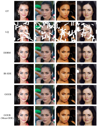
Figure 2: Qualitative comparison of the visual results of different inpainting methods on the CelebA-HQ datasets.

Image Deraining.

We have selected the Rain100H datasets (Yang et al., 2017) for our training and testing, which includes 1800 pairs of training data and 100 images for testing. It is important to note that in this task, similar to other deraining models, we present the PSNR and SSIM scores specifically on the Y channel (YCbCr space). The relevant experimental results can be viewed in the Table 2 and Figure 3. Similarly, in the deraining task, both models achieved SOTA results respectively. Visually, it can also be observed that our model excels in capturing details such as the moon, the sun and tree branches.

Table 2: Image Deraining. Qualitative comparison with the relevant baselines on Rain100H.

METHOD	PSNR$\uparrow$	SSIM$\uparrow$	LPIPS$\downarrow$	FID$\downarrow$
MPRNet(Zamir et al., 2021)	30.41	0.8906	0.158	61.59
M3SNet-32(Gao et al., 2023)	30.64	0.8920	0.154	60.26
MAXIM(Tu et al., 2022)	30.81	0.9027	0.133	58.72
MHNet(Gao and Dang, 2023)	31.08	0.8990	0.126	57.93
IR-SDE(Luo et al., 2023b)	31.65	0.9041	0.047	18.64
GOUB	31.96	0.9028	0.046	18.14
GOUB(Mean-ODE)	34.56	0.9414	0.077	32.83

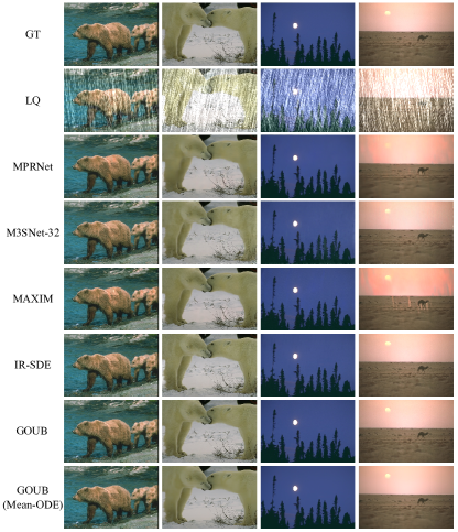
Figure 3: Qualitative comparison of the visual results of different deraining methods on the Rain100H dataset.

Image 4$\times$ Super-Resolution.

Single image super-resolution aims to recover a higher resolution and clearer version from a low-resolution image. We conducted training and evaluation on the DIV2K validation set for 4$\times$ upscaling (Agustsson and Timofte, 2017) and all low-resolution images were bicubically rescaled to the same size as their corresponding high-resolution images. The relevant experimental results can be viewed in the Table 3 and Figure 4.

Table 3: Image 4$\times$ Super-Resolution. Qualitative comparison with the relevant baselines on DIV2K.

METHOD	PSNR$\uparrow$	SSIM$\uparrow$	LPIPS$\downarrow$	FID$\downarrow$
DDRM(Kawar et al., 2022)	24.35	0.5927	0.364	78.71
IR-SDE(Luo et al., 2023b)	25.90	0.6570	0.231	45.36
GOUB	26.89	0.7478	0.220	20.85
GOUB(Mean-ODE)	28.50	0.8070	0.328	22.14

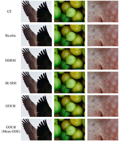
Figure 4: Qualitative comparison of the visual results of different super-resolution methods on the DIV2K dataset.

5 Related Works

Conditional Generation.

As previously highlighted, in the work of image restoration using diffusion models, the focus of some research has predominantly been on using low-quality images as conditional inputs $y$ to guide the generation process. They (Kawar et al., 2021; Saharia et al., 2022; Kawar et al., 2022; Chung et al., 2022b, a, 2023; Zhao et al., 2023; Murata et al., 2023; Feng et al., 2023) all endeavor to solve for the classifier $\log\nabla_{\mathbf{x}_{t}}p(\mathbf{y}\mid\mathbf{x}_{t})$, necessitating the incorporation of additional prior knowledge to model specific degradation processes which both complex and lacking in universality.

Diffusion Bridge.

This segment of work obviates the need for prior knowledge, constructing a diffusion bridge model from high-quality to low-quality images, thereby learning the degradation process. The previously mentioned approach (Liu et al., 2022a; De Bortoli et al., 2021; Su et al., 2022; Liu et al., 2023; Shi et al., 2023; Li et al., 2023; Zhou et al., 2023) falls into this classes and are characterized by the issues of significant computational expense in solution seeking and also not the optimal model architecture. Additionally, some models of flow category (Lipman et al., 2022; Liu et al., 2022b; Tong et al., 2023) also belong to the diffusion bridge models and similarly face the issue of substantial training overhead.

6 Discussion

The Doob’s h–transform of the generalized Ornstein-Uhlenbeck process, or the conditional GOU process has been an intriguing topic in previous applied mathematical research (Salminen, 1984; Cheridito et al., 2003; Heng et al., 2021). On account of the mean-reverting property of the GOU process, applying the h–transform makes it most straightforward to drive it towards a Dirac distribution in its steady state which is highly advantageous for its applications in the field of image restoration. In previous research on diffusion models, there has been limited focus on the cases of $\mathbf{f}$ or $g$, and used the VE process (Song et al., 2020) represented by NCSN (Song and Ermon, 2019) or the VP process (Song et al., 2020) represented by DDPM (Ho et al., 2020) typically.

In the subsequent discussions and experiments, we first demonstrate that the mathematical essence of several recent meaningful diffusion bridge models is the same (Li et al., 2023; Zhou et al., 2023; Liu et al., 2023) and they all represent Brownian bridge (Chow, 2009) models, details are provided in the Appendix B.1. We also found that the VE and VP processes are special cases of GOU, details are provided in the Appendix B.2. Therefore, we conduct experiments on VE Bridge (VEB) and VP Bridge (VPB) to demonstrate the optimality of our proposed GOUB model in the filed of image restoration. For $\mathbf{f}$ and $g$, we mainly refer to the settings in the original paper, while the model parameters remain consistent. The main results are shown in the Table 4, 5, 6 and Figure 5:

Table 4: Qualitative comparison with the different bridge model in inpainting task on CelebA-HQ datasets.

METHOD	PSNR$\uparrow$	SSIM$\uparrow$	LPIPS$\downarrow$	FID$\downarrow$
VEB (Li et al., 2023; Zhou et al., 2023; Liu et al., 2023)	27.75	0.8943	0.056	22.70
VPB (Zhou et al., 2023)	27.32	0.8841	0.049	19.87
GOUB	28.98	0.9067	0.037	4.30

Table 5: Qualitative comparison with the different bridge model in deraining task on Rain100H datasets.

METHOD	PSNR$\uparrow$	SSIM$\uparrow$	LPIPS$\downarrow$	FID$\downarrow$
VEB (Li et al., 2023; Zhou et al., 2023; Liu et al., 2023)	30.39	0.8975	0.059	28.54
VPB (Zhou et al., 2023)	30.89	0.8847	0.051	23.36
GOUB	31.96	0.9028	0.046	18.14

Table 6: Qualitative comparison with the different bridge model in 4$\times$ Super-Resolution task on DIV2K datasets.

METHOD	PSNR$\uparrow$	SSIM$\uparrow$	LPIPS$\downarrow$	FID$\downarrow$
VEB (Li et al., 2023; Zhou et al., 2023; Liu et al., 2023)	24.21	0.5808	0.384	36.55
VPB (Zhou et al., 2023)	25.40	0.6041	0.342	29.17
GOUB	26.89	0.7478	0.220	20.85

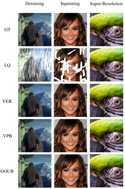
Figure 5: Qualitative comparison with the different bridge model in many tasks.

It can be seen that under the same configuration of model parameters, the performance of the GOUB is notably superior to the other two types of bridge models, which also highlights the importance of the choice of diffusion equation in diffusion models.

7 Conclusion

In this paper, we introduce Generalized Ornstein-Uhlenbeck Bridge (GOUB) model, a diffusion bridge model that applies the Doob’s h-transform to the GOU process. This model can address general image restoration tasks without the need for specific prior knowledge. Furthermore, we have uncovered the mathematical essence of many bridge models and empirically demonstrated the optimality of our proposed model. In addition, considering our unique mean parameterization mechanism, we proposed the Mean-ODE model. Experimental results indicate that both models achieve high competitive results in various tasks, including inpainting, deraining, and super-resolution. We believe that the exploration of diffusion equations and bridge models hold significant importance not only in the field of image restoration but also in advancing the study of generative diffusion models.

Appendix A Proof

A.1 Proof of Proposition 1

Proposition 1. Let $\mathbf{x}_{t}$ be a finite random variable describing by the given generalized Ornstein-Uhlenbeck process (4), suppose $\mathbf{x}_{T}=\bm{\mu}$, the evolution of its marginal distribution $p(\mathbf{x}_{t}\mid\mathbf{x}_{T})$ satisfies the following SDE:

$$\mathrm{d}\mathbf{x}_{t}=\left(\theta_{t}+g^{2}_{t}\frac{e^{-2\bar{\theta}_{t:T}}}{\bar{\sigma}_{t:T}^{2}}\right)(\mathbf{x}_{T}-\mathbf{x}_{t})\mathrm{d}t+g_{t}\mathrm{d}\mathbf{w}_{t},$$ (7)

additionally, the forward transition $p(\mathbf{x}_{t}\mid\mathbf{x}_{0},\mathbf{x}_{T})$ is given by:

$$p(\mathbf{x}_{t}\mid\mathbf{x}_{0},\mathbf{x}_{T}) =N(\mathbf{\bar{m}^{\prime}}_{t},\bar{\sigma}^{\prime 2}_{t}\mathbf{I})$$ (8)

$$=N\left(e^{-\bar{\theta}_{t}}\frac{\bar{\sigma}_{t:T}^{2}}{\bar{\sigma}_{T}^{2}}\mathbf{x}_{0}+\left[\left(1-e^{-\bar{\theta}_{t}}\right)\frac{\bar{\sigma}_{t:T}^{2}}{\bar{\sigma}_{T}^{2}}+e^{-2\bar{\theta}_{t:T}}\frac{\bar{\sigma}_{t}^{2}}{\bar{\sigma}_{T}^{2}}\right]\mathbf{x}_{T},\frac{\bar{\sigma}_{t}^{2}\bar{\sigma}_{t:T}^{2}}{\bar{\sigma}_{T}^{2}}\bm{I}\right)$$

Proof: Based on (5), we have:

$$p\left(\mathbf{x}_{t}\mid\mathbf{x}_{0}\right)=N\left(\mathbf{x}_{T}+\left(\mathbf{x}_{0}-\mathbf{x}_{T}\right)e^{-\bar{\theta}_{t}},\bar{\sigma}_{t}^{2}\bm{I}\right)$$ (19)

$$p\left(\mathbf{x}_{T}\mid\mathbf{x}_{t}\right)=N\left(\mathbf{x}_{T}+\left(\mathbf{x}_{t}-\mathbf{x}_{T}\right)e^{-\bar{\theta}_{t:T}},\bar{\sigma}_{t:T}^{2}\bm{I}\right)$$ (20)

$$p\left(\mathbf{x}_{T}\mid\mathbf{x}_{0}\right)=N\left(\mathbf{x}_{T}+\left(\mathbf{x}_{0}-\mathbf{x}_{T}\right)e^{-\bar{\theta}_{T}},\bar{\sigma}_{T}^{2}\bm{I}\right)$$ (21)

Firstly, the h function can be directly compute:

$$\mathbf{h}(\mathbf{x}_{t},t,\mathbf{x}_{T},T) =\nabla_{\mathbf{x}_{t}}\log p(\mathbf{x}_{T}\mid\mathbf{x}_{t})$$ (22)

$$=-\nabla_{\mathbf{x}_{t}}\frac{\left(\mathbf{x}_{t}-\mathbf{x}_{T}\right)^{2}e^{-2\bar{\theta}_{t:T}}}{2\sigma_{t:T}^{2}}$$

$$=(\mathbf{x}_{T}-\mathbf{x}_{t})\frac{e^{-2\bar{\theta}_{t:T}}}{\bar{\sigma}_{t:T}^{2}}$$

Therefore, followed by Doob’s h–transform (6), the SDE of marginal distribution $p(\mathbf{x}_{t}\mid\mathbf{x}_{T})$ satisfied is :

$$\mathrm{d}\mathbf{x}_{t} =\left[\mathbf{f}(\mathbf{x}_{t},t)+g^{2}_{t}\mathbf{h}(\mathbf{x}_{t},t,\mathbf{x}_{T},T)\right]\mathrm{d}t+g_{t}\mathrm{d}\mathbf{w}_{t}$$ (23)

$$=\left(\theta_{t}+g^{2}_{t}\frac{e^{-2\bar{\theta}_{t:T}}}{\bar{\sigma}_{t:T}^{2}}\right)(\mathbf{x}_{T}-\mathbf{x}_{t})\mathrm{d}t+g_{t}\mathrm{d}\mathbf{w}_{t}$$

Furthermore, we can derive the following transition probability of $\mathbf{x}_{t}$ using Bayes’ formula:

$$p(\mathbf{x}_{t}\mid\mathbf{x}_{0},\mathbf{x}_{T}) =\frac{p(\mathbf{x}_{T}\mid\mathbf{x}_{t},\mathbf{x}_{0})p(\mathbf{x}_{t}\mid\mathbf{x}_{0})}{p(\mathbf{x}_{T}\mid\mathbf{x}_{0})}$$ (24)

$$=\frac{p(\mathbf{x}_{T}\mid\mathbf{x}_{t})p(\mathbf{x}_{t}\mid\mathbf{x}_{0})}{p(\mathbf{x}_{T}\mid\mathbf{x}_{0})}$$

Since each component is independently and identically distributed (i.i.d), by considering a single dimension, we have:

$$p(\mathbf{x}_{t}\mid\mathbf{x}_{0},\mathbf{x}_{T}) \propto\frac{1}{\sqrt{2\pi}\bar{\sigma}_{t}\bar{\sigma}_{t:T}/\bar{\sigma}_{T}}\exp{-\left\{\frac{(\mathbf{x}_{t}-[\mathbf{x}_{T}+\left(\mathbf{x}_{0}-\mathbf{x}_{T}\right)e^{-\bar{\theta}_{t}}])^{2}}{2\bar{\sigma}_{t}^{2}}+\frac{(\mathbf{x}_{T}-[\mathbf{x}_{T}+\left(\mathbf{x}_{t}-\mathbf{x}_{T}\right)e^{-\bar{\theta}_{t:T}}])^{2}}{2\bar{\sigma}_{t:T}^{2}}\right\}}$$ (25)

$$=\frac{1}{\sqrt{2\pi}\bar{\sigma}_{t}\bar{\sigma}_{t:T}/\bar{\sigma}_{T}}\exp{-\left\{\frac{(\mathbf{x}_{t}-[\mathbf{x}_{T}+\left(\mathbf{x}_{0}-\mathbf{x}_{T}\right)e^{-\bar{\theta}_{t}}])^{2}}{2\bar{\sigma}_{t}^{2}}+\frac{\left(\mathbf{x}_{t}-\mathbf{x}_{T}\right)^{2}e^{-2\bar{\theta}_{t:T}}}{2\bar{\sigma}_{t:T}^{2}}\right\}}$$

$$\propto\frac{1}{\sqrt{2\pi}\bar{\sigma}_{t}\bar{\sigma}_{t:T}/\bar{\sigma}_{T}}\exp{-\left\{\left(\frac{1}{2\bar{\sigma}_{t}^{2}}+\frac{e^{-2\bar{\theta}_{t:T}}}{2\bar{\sigma}_{t:T}^{2}}\right)\mathbf{x}_{t}^{2}-\left(\frac{\mathbf{x}_{T}-\left(\mathbf{x}_{0}-\mathbf{x}_{T}\right)e^{-\bar{\theta}_{t}}}{\bar{\sigma}_{t}^{2}}+\frac{\mathbf{x}_{T}e^{-2\bar{\theta}_{t:T}}}{\bar{\sigma}_{t:T}^{2}}\right)\mathbf{x}_{t}\right\}}$$

Notice that:

$$\frac{1}{2\bar{\sigma}_{t}^{2}}+\frac{e^{-2\bar{\theta}_{t:T}}}{2\bar{\sigma}_{t:T}^{2}} =\frac{\sigma_{t:T}^{2}+\bar{\sigma}_{t}^{2}e^{-2\bar{\theta}_{t:T}}}{2\bar{\sigma}_{t}^{2}\bar{\sigma}_{t:T}^{2}}$$ (26)

$$=\frac{\lambda^{2}\left[(1-e^{-2\bar{\theta}_{t:T}})+(1-e^{-2\bar{\theta}_{t}})e^{-2\bar{\theta}_{t:T}}\right]}{2\bar{\sigma}_{t}^{2}\bar{\sigma}_{t:T}^{2}}$$

$$=\frac{\lambda^{2}\left[(1-e^{-2\bar{\theta}_{t:T}})+(e^{-2\bar{\theta}_{t:T}}-e^{-2\bar{\theta}_{T}})\right]}{2\bar{\sigma}_{t}^{2}\bar{\sigma}_{t:T}^{2}}$$

$$=\frac{\bar{\sigma}_{T}^{2}}{2\bar{\sigma}_{t}^{2}\bar{\sigma}_{t:T}^{2}}$$

Bringing it back to (25), squaring the terms and reorganizing the equation, we obtain:

$$p(\mathbf{x}_{t}\mid\mathbf{x}_{0},\mathbf{x}_{T}) \propto\frac{1}{\sqrt{2\pi}\bar{\sigma}_{t}\bar{\sigma}_{t:T}/\bar{\sigma}_{T}}\exp{-\left\{\frac{\bar{\sigma}_{T}^{2}}{2\bar{\sigma}_{t}^{2}\bar{\sigma}_{t:T}^{2}}\mathbf{x}_{t}^{2}-\left(\frac{\mathbf{x}_{T}-\left(\mathbf{x}_{0}-\mathbf{x}_{T}\right)e^{-\bar{\theta}_{t}}}{\bar{\sigma}_{t}^{2}}+\frac{\mathbf{x}_{T}e^{-2\bar{\theta}_{t:T}}}{\bar{\sigma}_{t:T}^{2}}\right)\mathbf{x}_{t}\right\}}$$ (27)

$$=\frac{1}{\sqrt{2\pi}\bar{\sigma}_{t}\bar{\sigma}_{t:T}/\bar{\sigma}_{T}}\exp{-\left\{\frac{\mathbf{x}_{t}^{2}-\left(\left[\mathbf{x}_{T}-\left(\mathbf{x}_{0}-\mathbf{x}_{T}\right)e^{-\bar{\theta}_{t}}\right]\frac{2\bar{\sigma}_{t:T}^{2}}{\bar{\sigma}_{T}^{2}}+e^{-2\bar{\theta}_{t:T}}\frac{2\bar{\sigma}_{t}^{2}}{\bar{\sigma}_{T}^{2}}\mathbf{x}_{T}\right)\mathbf{x}_{t}}{2(\bar{\sigma}_{t}\bar{\sigma}_{t:T}/\bar{\sigma}_{T})^{2}}\right\}}$$

$$\propto\frac{1}{\sqrt{2\pi}\bar{\sigma}_{t}\bar{\sigma}_{t:T}/\bar{\sigma}_{T}}\exp-\frac{\left\{\mathbf{x}_{t}-e^{-\bar{\theta}_{t}}\frac{\bar{\sigma}_{t:T}^{2}}{\bar{\sigma}_{T}^{2}}\mathbf{x}_{0}-\left[\left(1-e^{-\bar{\theta}_{t}}\right)\frac{\bar{\sigma}_{t:T}^{2}}{\bar{\sigma}_{T}^{2}}+e^{-2\bar{\theta}_{t:T}}\frac{\bar{\sigma}_{t}^{2}}{\bar{\sigma}_{T}^{2}}\right]\mathbf{x}_{T}\right\}^{2}}{2(\bar{\sigma}_{t}\bar{\sigma}_{t:T}/\bar{\sigma}_{T})^{2}}$$

$$=N\left(e^{-\bar{\theta}_{t}}\frac{\bar{\sigma}_{t:T}^{2}}{\bar{\sigma}_{T}^{2}}\mathbf{x}_{0}+\left[\left(1-e^{-\bar{\theta}_{t}}\right)\frac{\bar{\sigma}_{t:T}^{2}}{\bar{\sigma}_{T}^{2}}+e^{-2\bar{\theta}_{t:T}}\frac{\bar{\sigma}_{t}^{2}}{\bar{\sigma}_{T}^{2}}\right]\mathbf{x}_{T},\frac{\bar{\sigma}_{t}^{2}\bar{\sigma}_{t:T}^{2}}{\bar{\sigma}_{T}^{2}}\bm{I}\right)$$

This concludes the proof of the Proposition 1.

A.2 Proof of Proposition 3

Proposition 3. Let $\mathbf{x}_{t}$ be a finite random variable describing by the given generalized Ornstein-Uhlenbeck process (4), for a fixed $\mathbf{x}_{T}$, the expectation of log-likelihood $\mathbb{E}_{p(\mathbf{x}_{0})}[\log p_{\bm{\theta}}(\mathbf{x}_{0}\mid\mathbf{x}_{T})]$ possesses an Evidence Lower Bound (ELBO):

$$ELBO=\mathbb{E}_{p(\mathbf{x}_{0})}\left[\mathbb{E}_{p\left(\mathbf{x}_{1}\mid\mathbf{x}_{0}\right)}\left[\log p_{\bm{\theta}}\left(\mathbf{x}_{0}\mid\mathbf{x}_{1},\mathbf{x}_{T}\right)\right]-\sum_{t=2}^{T}{KL\left(p\left(\mathbf{x}_{t-1}\mid\mathbf{x}_{0},\mathbf{x}_{t},\mathbf{x}_{T}\right)||p_{\bm{\theta}}\left(\mathbf{x}_{t-1}\mid\mathbf{x}_{t},\mathbf{x}_{T}\right)\right)}\right]$$ (12)

Assuming $p_{\bm{\theta}}\left(\mathbf{x}_{t-1}\mid\mathbf{x}_{t},\mathbf{x}_{T}\right)$ is a Gaussian distribution with a constant variance $N(\bm{\mu}_{\bm{\theta},t-1},\sigma_{\bm{\theta},t-1}^{2}\bm{I})$, maximizing the ELBO is equivalent to minimizing:

$$\mathcal{L}=\mathbb{E}_{t,\mathbf{x}_{0},\mathbf{x}_{t},\mathbf{x}_{T}}\left[\frac{1}{2\sigma_{\bm{\theta},t-1}^{2}}\|\bm{\mu}_{t-1}-\bm{\mu}_{\bm{\theta},t-1}\|^{2}\right],$$ (13)

where $\bm{\mu}_{t-1}$ represents the mean of $p\left(\mathbf{x}_{t-1}\mid\mathbf{x}_{0},\mathbf{x}_{t},\mathbf{x}_{T}\right)$:

$$\bm{\mu}_{t-1}=\frac{1}{\bar{\sigma}^{\prime 2}_{t}}\left[\bar{\sigma}^{\prime 2}_{t-1}(\mathbf{x}_{t}-b\mathbf{x}_{T})a+(\bar{\sigma}^{\prime 2}_{t}-\bar{\sigma}^{\prime 2}_{t-1}a^{2})\mathbf{\bar{m}^{\prime}}_{t}\right],$$ (14)

where,

$$a=\frac{e^{-\bar{\theta}_{t-1:t}}\bar{\sigma}_{t:T}^{2}}{\bar{\sigma}_{t-1:T}^{2}},$$

$$b=\frac{1}{\bar{\sigma}_{T}^{2}}\left\{(1-e^{-\bar{\theta}_{t}})\bar{\sigma}^{2}_{t:T}+e^{-2\bar{\theta}_{t:T}}\bar{\sigma}_{t}^{2}-\left[(1-e^{-\bar{\theta}_{t-1}})\bar{\sigma}^{2}_{t-1:T}+e^{-2\bar{\theta}_{t-1:T}}\bar{\sigma}_{t-1}^{2}\right]a\right\}$$

Proof: Firstly, followed by the theorem in DDPM (Ho et al., 2020):

$$\mathbb{E}_{p(\mathbf{x}_{0})}\left[\log p(\mathbf{x}_{0})\right]\geq \mathbb{E}_{p(\mathbf{x}_{0})}\Bigg{[}-KL(p(\mathbf{x}_{T}\mid\mathbf{x}_{0})||p(\mathbf{x}_{T}))+\mathbb{E}_{p\left(\mathbf{x}_{1}\mid\mathbf{x}_{0}\right)}\left[\log p_{\bm{\theta}}\left(\mathbf{x}_{0}\mid\mathbf{x}_{1}\right)\right]-\Bigg{.}$$ (28)

$$\Bigg{.}\sum_{t=2}^{T}{KL\left(p\left(\mathbf{x}_{t-1}\mid\mathbf{x}_{0},\mathbf{x}_{t}\right)||p_{\bm{\theta}}\left(\mathbf{x}_{t-1}\mid\mathbf{x}_{t}\right)\right)}\Bigg{]}$$

Similarly, we have:

$$\mathbb{E}_{p(\mathbf{x}_{0})}[\log p_{\bm{\theta}}(\mathbf{x}_{0}\mid\mathbf{x}_{T})] \geq\mathbb{E}_{p(\mathbf{x}_{0})}\Bigg{[}-KL(p(\mathbf{x}_{T}\mid\mathbf{x}_{0},\mathbf{x}_{T})||p(\mathbf{x}_{T}\mid\mathbf{x}_{T}))+\mathbb{E}_{p\left(\mathbf{x}_{1}\mid\mathbf{x}_{0}\right)}\left[\log p_{\bm{\theta}}\left(\mathbf{x}_{0}\mid\mathbf{x}_{1},\mathbf{x}_{T}\right)\right]\Bigg{.}$$ (29)

$$\Bigg{.}\quad-\sum_{t=2}^{T}{KL\left(p\left(\mathbf{x}_{t-1}\mid\mathbf{x}_{0},\mathbf{x}_{t},\mathbf{x}_{T}\right)||p_{\bm{\theta}}\left(\mathbf{x}_{t-1}\mid\mathbf{x}_{t},\mathbf{x}_{T}\right)\right)}\Bigg{]}$$

$$=\mathbb{E}_{p(\mathbf{x}_{0})}\left[\mathbb{E}_{p\left(\mathbf{x}_{1}\mid\mathbf{x}_{0}\right)}\left[\log p_{\bm{\theta}}\left(\mathbf{x}_{0}\mid\mathbf{x}_{1},\mathbf{x}_{T}\right)\right]-\sum_{t=2}^{T}{KL\left(p\left(\mathbf{x}_{t-1}\mid\mathbf{x}_{0},\mathbf{x}_{t},\mathbf{x}_{T}\right)||p_{\bm{\theta}}\left(\mathbf{x}_{t-1}\mid\mathbf{x}_{t},\mathbf{x}_{T}\right)\right)}\right]$$

$$=ELBO$$

From Bayes’ formula, we can infer that:

$$p\left(\mathbf{x}_{t-1}\mid\mathbf{x}_{0},\mathbf{x}_{t},\mathbf{x}_{T}\right) =\frac{p(\mathbf{x}_{t}\mid\mathbf{x}_{0},\mathbf{x}_{t-1},\mathbf{x}_{T})p(\mathbf{x}_{t-1}\mid\mathbf{x}_{0},\mathbf{x}_{T})}{p(\mathbf{x}_{t}\mid\mathbf{x}_{0},\mathbf{x}_{T})}$$ (30)

$$=\frac{p(\mathbf{x}_{t}\mid\mathbf{x}_{t-1},\mathbf{x}_{T})p(\mathbf{x}_{t-1}\mid\mathbf{x}_{0},\mathbf{x}_{T})}{p(\mathbf{x}_{t}\mid\mathbf{x}_{0},\mathbf{x}_{T})}$$

Since $p(\mathbf{x}_{t-1}\mid\mathbf{x}_{0},\mathbf{x}_{T})$ and $p(\mathbf{x}_{t}\mid\mathbf{x}_{0},\mathbf{x}_{T})$ are Gaussian distributions (8), by employing the reparameterization technique:

$$\mathbf{x}_{t-1} =e^{-\bar{\theta}_{t-1}}\frac{\bar{\sigma}_{t-1:T}^{2}}{\bar{\sigma}_{T}^{2}}\mathbf{x}_{0}+\left[\left(1-e^{-\bar{\theta}_{t-1}}\right)\frac{\bar{\sigma}_{t-1:T}^{2}}{\bar{\sigma}_{T}^{2}}+e^{-2\bar{\theta}_{t-1:T}}\frac{\bar{\sigma}_{t-1}^{2}}{\bar{\sigma}_{T}^{2}}\right]\mathbf{x}_{T}+\bar{\sigma}^{\prime}_{t-1}\bm{\epsilon}_{t-1}$$ (31)

$$=m(t-1)\mathbf{x}_{0}+n(t-1)\mathbf{x}_{T}+\bar{\sigma}^{\prime}_{t-1}\bm{\epsilon}_{t-1}$$

$$\mathbf{x}_{t} =e^{-\bar{\theta}_{t}}\frac{\bar{\sigma}_{t:T}^{2}}{\bar{\sigma}_{T}^{2}}\mathbf{x}_{0}+\left[\left(1-e^{-\bar{\theta}_{t}}\right)\frac{\bar{\sigma}_{t:T}^{2}}{\bar{\sigma}_{T}^{2}}+e^{-2\bar{\theta}_{t:T}}\frac{\bar{\sigma}_{t}^{2}}{\bar{\sigma}_{T}^{2}}\right]\mathbf{x}_{T}+\bar{\sigma}^{\prime}_{t}\bm{\epsilon}_{t}$$

$$=m(t)\mathbf{x}_{0}+n(t)\mathbf{x}_{T}+\bar{\sigma}^{\prime}_{t}\bm{\epsilon}_{t}$$

Therefore,

$$\mathbf{x}_{t} =\frac{m(t)}{m(t-1)}\mathbf{x}_{t-1}+\left[n(t)-\frac{m(t)}{m(t-1)}n(t-1)\right]\mathbf{x}_{T}+\sqrt{\bar{\sigma}^{\prime 2}_{t}-\frac{m(t)^{2}}{m(t-1)^{2}}\bar{\sigma}^{\prime 2}_{t-1}}\bm{\epsilon}$$ (32)

$$=a\mathbf{x}_{t-1}+\left[n(t)-an(t-1)\right]\mathbf{x}_{T}+\sqrt{\bar{\sigma}^{\prime 2}_{t}-a^{2}\bar{\sigma}^{\prime 2}_{t-1}}\bm{\epsilon}$$

$$=a\mathbf{x}_{t-1}+b\mathbf{x}_{T}+\sqrt{\bar{\sigma}^{\prime 2}_{t}-a^{2}\bar{\sigma}^{\prime 2}_{t-1}}\bm{\epsilon}$$

Thus, $p(\mathbf{x}_{t}\mid\mathbf{x}_{t-1},\mathbf{x}_{T})=N(a\mathbf{x}_{t-1}+b\mathbf{x}_{T},\left(\bar{\sigma}^{\prime 2}_{t}-a^{2}\bar{\sigma}^{\prime 2}_{t-1}\right)\bm{I})$ is also a Gaussian distribution. Bring it back to equation (30) we can easily obtain :

$$\bm{\mu}_{t-1}=\frac{1}{\bar{\sigma}^{\prime 2}_{t}}\left[\bar{\sigma}^{\prime 2}_{t-1}(\mathbf{x}_{t}-b\mathbf{x}_{T})a+(\bar{\sigma}^{\prime 2}_{t}-\bar{\sigma}^{\prime 2}_{t-1}a^{2})\mathbf{\bar{m}^{\prime}}_{t}\right],$$ (14)

Accordingly,

$$KL\left(p\left(\mathbf{x}_{t-1}\mid\mathbf{x}_{0},\mathbf{x}_{t},\mathbf{x}_{T}\right)||p_{\bm{\theta}}\left(\mathbf{x}_{t-1}\mid\mathbf{x}_{t},\mathbf{x}_{T}\right)\right)$$ (33)

$$= \mathbb{E}_{p\left(\mathbf{x}_{t-1}\mid\mathbf{x}_{0},\mathbf{x}_{t},\mathbf{x}_{T}\right)}\left[\log\frac{\frac{1}{\sqrt{2\pi}\sigma_{t-1}}e^{-(\mathbf{x}_{t-1}-\bm{\mu}_{t-1})^{2}/{2\sigma_{t-1}^{2}}}}{\frac{1}{\sqrt{2\pi}\sigma_{\bm{\theta},t-1}}e^{-(\mathbf{x}_{t-1}-\bm{\mu}_{\bm{\theta},t-1})^{2}/{2\sigma_{\bm{\theta},t-1}^{2}}}}\right]$$

$$= \mathbb{E}_{p\left(\mathbf{x}_{t-1}\mid\mathbf{x}_{0},\mathbf{x}_{t},\mathbf{x}_{T}\right)}\left[\log\sigma_{\bm{\theta},t-1}-\log\sigma_{t-1}-(\mathbf{x}_{t-1}-\bm{\mu}_{t-1})^{2}/{2\sigma^{2}_{t-1}}+(\mathbf{x}_{t-1}-\bm{\mu}_{\bm{\theta},t-1})^{2}/{2\sigma_{\bm{\theta},t-1}^{2}}\right]$$

$$= \log\sigma_{\bm{\theta},t-1}-\log\sigma_{t-1}-\frac{1}{2}+\frac{\sigma_{t-1}^{2}}{2\sigma_{\bm{\theta},t-1}^{2}}+\frac{(\bm{\mu}_{t-1}-\bm{\mu}_{\bm{\theta},t-1})^{2}}{2\sigma_{\bm{\theta},t-1}^{2}}$$

Ignoring unlearnable constant, the training object that involves minimizing the negative ELBO is :

$$\mathcal{L}=\mathbb{E}_{t,\mathbf{x}_{0},\mathbf{x}_{t},\mathbf{x}_{T}}\left[\frac{1}{2\sigma_{\bm{\theta},t-1}^{2}}\|\bm{\mu}_{t-1}-\bm{\mu}_{\bm{\theta},t-1}\|^{2}\right],$$ (34)

This concludes the proof of the Proposition 3.

Appendix B Theoretical Results

B.1 Brownian Bridge

In this section, we will show the mathematical essence of some other bridge models, some of which are all equivalent.

Proposition 4.

The mathematical essence of BBDM (Li et al., 2023), DDBM (VE) (Zhou et al., 2023) and $I^{2}$SB (Liu et al., 2023) are all equivalent to Brownian bridge.

Proof: Firstly, it is easy to understand that BBDM uses the Brownian bridge as its fundamental model architecture.

The DDBM (VE) model is derived as the Doob’s h–transform of VE-SDE, and we begin by specifying the SDE:

$$\mathrm{d}\mathbf{x}_{t}=g_{t}\mathrm{d}\mathbf{w}_{t}$$ (35)

Its transition probability is given by:

$$p\left(\mathbf{x}_{t}\mid\mathbf{x}_{s}\right)=N(\mathbf{x}_{s},g_{t}^{2}(t-s))$$ (36)

Since, the h–function of SDE (35) is:

$$\mathbf{h}(\mathbf{x}_{t},t,\mathbf{x}_{T},T) =\nabla_{\mathbf{x}_{t}}\log p(\mathbf{x}_{T}\mid\mathbf{x}_{t})$$ (37)

$$=\frac{\mathbf{x}_{T}-\mathbf{x}_{t}}{g_{t}^{2}(T-t)}$$

Therefore, the Doob’s h–transform of (35) is:

$$\mathrm{d}\mathbf{x}_{t}=\frac{\mathbf{x}_{T}-\mathbf{x}_{t}}{(T-t)}\mathrm{d}t+g_{t}\mathrm{d}\mathbf{w}_{t}$$ (38)

That is the definition of Brownian bridge. Hence, DDBM (VE) is a Brownian bridge model.

Furthermore, the transition kernel of (38) is:

$$p(\mathbf{x}_{t}\mid\mathbf{x}_{0},\mathbf{x}_{T}) =\frac{p(\mathbf{x}_{T}\mid\mathbf{x}_{t},\mathbf{x}_{0})p(\mathbf{x}_{t}\mid\mathbf{x}_{0})}{p(\mathbf{x}_{T}\mid\mathbf{x}_{0})}$$ (39)

$$=\frac{p(\mathbf{x}_{T}\mid\mathbf{x}_{t})p(\mathbf{x}_{t}\mid\mathbf{x}_{0})}{p(\mathbf{x}_{T}\mid\mathbf{x}_{0})}$$

$$=\frac{N(\mathbf{x}_{t},g_{t}^{2}(T-t))N(\mathbf{x}_{0},g_{t}^{2}t)}{N(\mathbf{x}_{0},g_{T}^{2}T)}$$

$$=N\left(\left(1-\frac{t}{T}\right)\mathbf{x}_{0}+\frac{t}{T}\mathbf{x}_{T},\frac{t(T-t)}{T}g_{t}^{2}\bm{I}\right)$$

This precisely corresponds to the sampling process of $\mathrm{I}^{2}$SB , thus confirming that $\mathrm{I}^{2}$SB also represents a Brownian bridge.

This concludes the proof of the Proposition 4.

B.2 Connections Between GOU, VE and VP

The following proposition will show us that both VE and VP process are special cases of GOU process:

Proposition 5.

For a given GOU process (4), there exists relationships:

$$\lim_{\theta_{t}\rightarrow 0}\text{GOU}=\text{VE}$$ (40)

$$\lim_{\bm{\mu}\rightarrow 0,\lambda\rightarrow 1}\text{GOU}=\text{VP}$$

Proof: It’s easy to know:

$$\lim_{\theta_{t}\rightarrow 0}\text{GOU} =\lim_{\theta_{t}\rightarrow 0}\left\{\mathrm{d}\mathbf{x}_{t}=\theta_{t}\left(\bm{\mu}-\mathbf{x}_{t}\right)\mathrm{d}t+g_{t}\mathrm{d}\mathbf{w}_{t}\right\}$$ (41)

$$=\lim_{\theta_{t}\rightarrow 0}\left\{\mathrm{d}\mathbf{x}_{t}=g_{t}\mathrm{d}\mathbf{w}_{t}\right\}$$

$$=\text{VE}$$

Where $g_{t}$ will be controlled by $\lambda^{2}$.

Besides, we have:

$$\lim_{\bm{\mu}\rightarrow 0,\lambda\rightarrow 1}\text{GOU} =\lim_{\bm{\mu}\rightarrow 0,\lambda\rightarrow 1}\left\{\mathrm{d}\mathbf{x}_{t}=\theta_{t}\left(\bm{\mu}-\mathbf{x}_{t}\right)\mathrm{d}t+g_{t}\mathrm{d}\mathbf{w}_{t}\right\}$$ (42)

$$=\lim_{\bm{\mu}\rightarrow 0,\lambda\rightarrow 1}\left\{\mathrm{d}\mathbf{x}_{t}=\theta_{t}\bm{\mu}\mathrm{d}t-\theta_{t}\mathbf{x}_{t}\mathrm{d}t+g_{t}\mathrm{d}\mathbf{w}_{t}\right\}$$

$$=\lim_{\bm{\mu}\rightarrow 0,\lambda\rightarrow 1}\left\{\mathrm{d}\mathbf{x}_{t}=-\frac{1}{2}g_{t}^{2}\mathbf{x}_{t}\mathrm{d}t+g_{t}\mathrm{d}\mathbf{w}_{t}\right\}$$

$$=\text{VP}$$

Where $g_{t}$ will be controlled by $\theta_{t}$.

This concludes the proof of the Proposition 5.

Appendix C GOU Process

Theorem 1.

For a given GOU process:

$$\mathrm{d}\mathbf{x}_{t}=\theta_{t}\left(\bm{\mu}-\mathbf{x}_{t}\right)\mathrm{d}t+g_{t}\mathrm{d}\mathbf{w}_{t}$$ (4)

where $\bm{\mu}$ is a given state vector, $\theta_{t}$ denotes a scalar drift coefficient and $g_{t}$ represents the diffusion coefficient. It possesses a closed-form analytical solution:

$$p\left(\mathbf{x}_{t}\mid\mathbf{x}_{s}\right)=N\left(\bm{\mu}+\left(\mathbf{x}_{s}-\bm{\mu}\right)e^{-\bar{\theta}_{s:t}},\frac{g^{2}_{t}}{2\theta_{t}}\left(1-e^{-2\bar{\theta}_{s:t}}\right)\bm{I}\right),\qquad\bar{\theta}_{s:t}=\int_{s}^{t}{\theta_{z}dz}$$ (5)

Proof: Writing:

$$\mathbf{f}(\mathbf{x}_{t},t)=\mathbf{x}_{t}e^{\bar{\theta}_{t}}$$ (43)

Using Ito differential formula, we get:

$$\mathrm{d}\mathbf{f}(\mathbf{x}_{t},t) =\mathbf{x}_{t}\theta_{t}e^{\bar{\theta}_{t}}\mathrm{d}t+e^{\bar{\theta}_{t}}\mathrm{d}\mathbf{x}_{t}$$ (44)

$$=\mathbf{x}_{t}\theta_{t}e^{\bar{\theta}_{t}}\mathrm{d}t+e^{\bar{\theta}_{t}}\left[\theta_{t}\left(\bm{\mu}-\mathbf{x}_{t}\right)\mathrm{d}t+g_{t}\mathrm{d}\mathbf{w}_{t}\right]$$

$$=e^{\bar{\theta}_{t}}\theta_{t}\bm{\mu}+e^{\bar{\theta}_{t}}g_{t}\mathrm{d}\mathbf{w}_{t}$$

Integrating from $s$ to $t$ we get:

$$\mathbf{x}_{t}e^{\bar{\theta}_{t}}-\mathbf{x}_{s}e^{\bar{\theta}_{s}} =\int_{s}^{t}e^{\bar{\theta}_{z}}\theta_{z}\bm{\mu}\mathrm{d}z+\int_{s}^{t}e^{\bar{\theta}_{z}}g_{z}\mathrm{d}\mathbf{w}_{z}$$ (45)

$$=\left(e^{\bar{\theta}_{t}}-e^{\bar{\theta}_{s}}\right)\bm{\mu}+\int_{s}^{t}e^{\bar{\theta}_{z}}g_{z}\mathrm{d}\mathbf{w}_{z}$$

It’s obviously that the transition kernel is a Gaussian distribution. Since $\mathrm{d}\mathbf{w}_{z}\sim N(\mathbf{0},\mathrm{d}z\bm{I})$, we have:

$$\int_{s}^{t}e^{\bar{\theta}_{z}}g_{z}\mathrm{d}\mathbf{w}_{z} =N\left(\mathbf{0},\int_{s}^{t}e^{2\bar{\theta}_{z}}g^{2}_{z}\mathrm{d}z\bm{I}\right)$$ (46)

$$=N\left(\mathbf{0},\lambda^{2}\int_{s}^{t}e^{2\bar{\theta}_{z}}2\theta_{t}\mathrm{d}z\bm{I}\right)$$

$$=N\left(\mathbf{0},\lambda^{2}\left(e^{2\bar{\theta}_{t}}-e^{2\bar{\theta}_{s}}\right)\bm{I}\right)$$

Therefore:

$$\mathbf{x}_{t}e^{\bar{\theta}_{t}}-\mathbf{x}_{s}e^{\bar{\theta}_{s}}=\left(e^{\bar{\theta}_{t}}-e^{\bar{\theta}_{s}}\right)\bm{\mu}+N\left(\mathbf{0},\lambda^{2}\left(e^{2\bar{\theta}_{t}}-e^{2\bar{\theta}_{s}}\right)\bm{I}\right)$$ (47)

$$\mathbf{x}_{t}=\bm{\mu}+\left(\mathbf{x}_{s}-\bm{\mu}\right)e^{-\bar{\theta}_{s:t}}+\left(\mathbf{0},\frac{g^{2}_{t}}{2\theta_{t}}\left(1-e^{-2\bar{\theta}_{s:t}}\right)\bm{I}\right)$$

This concludes the proof of the Theorem 1.

Appendix D Doob’s h–transform

Theorem 2.

For a given SDE:

$$\mathrm{d}\mathbf{x}_{t}=\mathbf{f}\left(\mathbf{x}_{t},t\right)\mathrm{d}t+g_{t}\mathrm{d}\mathbf{w}_{t},\qquad\mathbf{x}_{0}\sim p\left(\mathbf{x}_{0}\right),$$ (1)

For a fixed $\mathbf{x}_{T}$, the evolution of conditional probability $p(\mathbf{x}_{t}\mid\mathbf{x}_{T})$ follows:

$$\mathrm{d}\mathbf{x}_{t}=\left[\mathbf{f}(\mathbf{x}_{t},t)+g^{2}_{t}\mathbf{h}(\mathbf{x}_{t},t,\mathbf{x}_{T},T)\right]\mathrm{d}t+g_{t}\mathrm{d}\mathbf{w}_{t},\qquad\mathbf{x}_{0}\sim p\left(\mathbf{x}_{0}\mid\mathbf{x}_{T}\right),$$ (6)

where $\mathbf{h}(\mathbf{x}_{t},t,\mathbf{x}_{T},T)=\nabla_{\mathbf{x}_{t}}\log p(\mathbf{x}_{T}\mid\mathbf{x}_{t})$.

Proof: $p(\mathbf{x}_{t}\mid\mathbf{x}_{0})$ satisfies Kolmogorov Forward Equation (KFE) also called Fokker-Planck equation (Risken and Risken, 1996):

$$\frac{\partial}{\partial t}p(\mathbf{x}_{t}\mid\mathbf{x}_{0})=-\nabla_{\mathbf{x}_{t}}\cdot\left[\mathbf{f}(\mathbf{x}_{t},t)p(\mathbf{x}_{t}\mid\mathbf{x}_{0})\right]+\frac{1}{2}g^{2}_{t}\nabla_{\mathbf{x}_{t}}\cdot\nabla_{\mathbf{x}_{t}}p(\mathbf{x}_{t}\mid\mathbf{x}_{0})$$ (48)

Similarly, $p(\mathbf{x}_{T}\mid\mathbf{x}_{t})$ satisfies Kolmogorov Backward Equation (KBE) (Risken and Risken, 1996):

$$-\frac{\partial}{\partial t}p(\mathbf{x}_{T}\mid\mathbf{x}_{t})=\mathbf{f}(\mathbf{x}_{t},t)\cdot\nabla_{\mathbf{x}_{t}}p(\mathbf{x}_{T}\mid\mathbf{x}_{t})+\frac{1}{2}g^{2}_{t}\nabla_{\mathbf{x}_{t}}\cdot\nabla_{\mathbf{x}_{t}}p(\mathbf{x}_{T}\mid\mathbf{x}_{t})$$ (49)

Using Bayes’ rule, we have:

$$p(\mathbf{x}_{t}\mid\mathbf{x}_{0},\mathbf{x}_{T}) =\frac{p(\mathbf{x}_{T}\mid\mathbf{x}_{t},\mathbf{x}_{0})p(\mathbf{x}_{t}\mid\mathbf{x}_{0})}{p(\mathbf{x}_{T}\mid\mathbf{x}_{0})}$$ (50)

$$=\frac{p(\mathbf{x}_{T}\mid\mathbf{x}_{t})p(\mathbf{x}_{t}\mid\mathbf{x}_{0})}{p(\mathbf{x}_{T}\mid\mathbf{x}_{0})}$$

Therefore, the derivative of conditional transition probability $p(\mathbf{x}_{t}\mid\mathbf{x}_{0},\mathbf{x}_{T})$ with time follows:

$$\frac{\partial}{\partial t}p(\mathbf{x}_{t}\mid\mathbf{x}_{0},\mathbf{x}_{T}) =\frac{p(\mathbf{x}_{t}\mid\mathbf{x}_{0})}{p(\mathbf{x}_{T}\mid\mathbf{x}_{0})}\frac{\partial}{\partial t}p(\mathbf{x}_{T}\mid\mathbf{x}_{t})+\frac{p(\mathbf{x}_{T}\mid\mathbf{x}_{t})}{p(\mathbf{x}_{T}\mid\mathbf{x}_{0})}\frac{\partial}{\partial t}p(\mathbf{x}_{t}\mid\mathbf{x}_{0})$$ (51)

$$=\frac{p(\mathbf{x}_{t}\mid\mathbf{x}_{0})}{p(\mathbf{x}_{T}\mid\mathbf{x}_{0})}\left[-\mathbf{f}(\mathbf{x}_{t},t)\cdot\nabla_{\mathbf{x}_{t}}p(\mathbf{x}_{T}\mid\mathbf{x}_{t})-\frac{1}{2}g^{2}_{t}\nabla_{\mathbf{x}_{t}}\cdot\nabla_{\mathbf{x}_{t}}p(\mathbf{x}_{T}\mid\mathbf{x}_{t})\right]$$

$$\quad+\frac{p(\mathbf{x}_{T}\mid\mathbf{x}_{t})}{p(\mathbf{x}_{T}\mid\mathbf{x}_{0})}\left\{-\nabla_{\mathbf{x}_{t}}\cdot\left[\mathbf{f}(\mathbf{x}_{t},t)p(\mathbf{x}_{t}\mid\mathbf{x}_{0})\right]+\frac{1}{2}g^{2}_{t}\nabla_{\mathbf{x}_{t}}\cdot\nabla_{\mathbf{x}_{t}}p(\mathbf{x}_{t}\mid\mathbf{x}_{0})\right\}$$

$$=-\left[\frac{p(\mathbf{x}_{t}\mid\mathbf{x}_{0})}{p(\mathbf{x}_{T}\mid\mathbf{x}_{0})}\mathbf{f}(\mathbf{x}_{t},t)\cdot\nabla_{\mathbf{x}_{t}}p(\mathbf{x}_{T}\mid\mathbf{x}_{t})+\frac{p(\mathbf{x}_{T}\mid\mathbf{x}_{t})}{p(\mathbf{x}_{T}\mid\mathbf{x}_{0})}\mathbf{f}(\mathbf{x}_{t},t)\nabla_{\mathbf{x}_{t}}p(\mathbf{x}_{t}\mid\mathbf{x}_{0})\right.$$

$$\quad\left.+\frac{p(\mathbf{x}_{T}\mid\mathbf{x}_{t})}{p(\mathbf{x}_{T}\mid\mathbf{x}_{0})}p(\mathbf{x}_{t}\mid\mathbf{x}_{0})\nabla_{\mathbf{x}_{t}}\cdot\mathbf{f}(\mathbf{x}_{t},t)\right]$$

$$\quad+\frac{1}{2}g_{t}^{2}\left[\frac{p(\mathbf{x}_{T}\mid\mathbf{x}_{t})}{p(\mathbf{x}_{T}\mid\mathbf{x}_{0})}\nabla_{\mathbf{x}_{t}}\cdot\nabla_{\mathbf{x}_{t}}p(\mathbf{x}_{t}\mid\mathbf{x}_{0})-\frac{p(\mathbf{x}_{t}\mid\mathbf{x}_{0})}{p(\mathbf{x}_{T}\mid\mathbf{x}_{0})}\nabla_{\mathbf{x}_{t}}\cdot\nabla_{\mathbf{x}_{t}}p(\mathbf{x}_{T}\mid\mathbf{x}_{t})\right]$$

$$=-\left[\mathbf{f}(\mathbf{x}_{t},t)\cdot\nabla_{\mathbf{x}_{t}}p(\mathbf{x}_{t}\mid\mathbf{x}_{0},\mathbf{x}_{T})+p(\mathbf{x}_{t}\mid\mathbf{x}_{0},\mathbf{x}_{T})\cdot\nabla_{\mathbf{x}_{t}}\mathbf{f}(\mathbf{x}_{t},t)\right]$$

$$\quad+\frac{1}{2}g_{t}^{2}\left[\frac{p(\mathbf{x}_{T}\mid\mathbf{x}_{t})}{p(\mathbf{x}_{T}\mid\mathbf{x}_{0})}\nabla_{\mathbf{x}_{t}}\cdot\nabla_{\mathbf{x}_{t}}p(\mathbf{x}_{t}\mid\mathbf{x}_{0})-\frac{p(\mathbf{x}_{t}\mid\mathbf{x}_{0})}{p(\mathbf{x}_{T}\mid\mathbf{x}_{0})}\nabla_{\mathbf{x}_{t}}\cdot\nabla_{\mathbf{x}_{t}}p(\mathbf{x}_{T}\mid\mathbf{x}_{t})\right]$$

$$=-\nabla_{\mathbf{x}_{t}}\cdot\left[\mathbf{f}(\mathbf{x}_{t},t)p(\mathbf{x}_{t}\mid\mathbf{x}_{0},\mathbf{x}_{T})\right]$$

$$\quad+\frac{1}{2}g_{t}^{2}\left[\frac{p(\mathbf{x}_{T}\mid\mathbf{x}_{t})}{p(\mathbf{x}_{T}\mid\mathbf{x}_{0})}\nabla_{\mathbf{x}_{t}}\cdot\nabla_{\mathbf{x}_{t}}p(\mathbf{x}_{t}\mid\mathbf{x}_{0})-\frac{p(\mathbf{x}_{t}\mid\mathbf{x}_{0})}{p(\mathbf{x}_{T}\mid\mathbf{x}_{0})}\nabla_{\mathbf{x}_{t}}\cdot\nabla_{\mathbf{x}_{t}}p(\mathbf{x}_{T}\mid\mathbf{x}_{t})\right]$$

For the second term, we have:

$$\frac{1}{2}g_{t}^{2}\left[\frac{p(\mathbf{x}_{T}\mid\mathbf{x}_{t})}{p(\mathbf{x}_{T}\mid\mathbf{x}_{0})}\nabla_{\mathbf{x}_{t}}\cdot\nabla_{\mathbf{x}_{t}}p(\mathbf{x}_{t}\mid\mathbf{x}_{0})-\frac{p(\mathbf{x}_{t}\mid\mathbf{x}_{0})}{p(\mathbf{x}_{T}\mid\mathbf{x}_{0})}\nabla_{\mathbf{x}_{t}}\cdot\nabla_{\mathbf{x}_{t}}p(\mathbf{x}_{T}\mid\mathbf{x}_{t})\right]$$ (52)

$$= \frac{1}{2}g_{t}^{2}\left[\frac{p(\mathbf{x}_{T}\mid\mathbf{x}_{t})}{p(\mathbf{x}_{T}\mid\mathbf{x}_{0})}\nabla_{\mathbf{x}_{t}}\cdot\nabla_{\mathbf{x}_{t}}p(\mathbf{x}_{t}\mid\mathbf{x}_{0})+\frac{1}{p(\mathbf{x}_{T}\mid\mathbf{x}_{0})}\nabla_{\mathbf{x}_{t}}p(\mathbf{x}_{T}\mid\mathbf{x}_{t})\cdot\nabla_{\mathbf{x}_{t}}\ p(\mathbf{x}_{t}\mid\mathbf{x}_{0})\right.$$

$$\left.+\frac{1}{p(\mathbf{x}_{T}\mid\mathbf{x}_{0})}\nabla_{\mathbf{x}_{t}}p(\mathbf{x}_{T}\mid\mathbf{x}_{t})\cdot\nabla_{\mathbf{x}_{t}}\ p(\mathbf{x}_{t}\mid\mathbf{x}_{0})+\frac{p(\mathbf{x}_{t}\mid\mathbf{x}_{0})}{p(\mathbf{x}_{T}\mid\mathbf{x}_{0})}\nabla_{\mathbf{x}_{t}}\cdot\nabla_{\mathbf{x}_{t}}p(\mathbf{x}_{T}\mid\mathbf{x}_{t})\right]$$

$$-g_{t}^{2}\left[\frac{1}{p(\mathbf{x}_{T}\mid\mathbf{x}_{0})}\nabla_{\mathbf{x}_{t}}p(\mathbf{x}_{T}\mid\mathbf{x}_{t})\cdot\nabla_{\mathbf{x}_{t}}\ p(\mathbf{x}_{t}\mid\mathbf{x}_{0})+\frac{p(\mathbf{x}_{t}\mid\mathbf{x}_{0})}{p(\mathbf{x}_{T}\mid\mathbf{x}_{0})}\nabla_{\mathbf{x}_{t}}\cdot\nabla_{\mathbf{x}_{t}}p(\mathbf{x}_{T}\mid\mathbf{x}_{t})\right]$$

$$= \frac{1}{2}g_{t}^{2}\left[\frac{1}{p(\mathbf{x}_{T}\mid\mathbf{x}_{0})}\nabla_{\mathbf{x}_{t}}\cdot\left[p(\mathbf{x}_{T}\mid\mathbf{x}_{t})\nabla_{\mathbf{x}_{t}}p(\mathbf{x}_{t}\mid\mathbf{x}_{0})\right]+\frac{1}{p(\mathbf{x}_{T}\mid\mathbf{x}_{0})}\nabla_{\mathbf{x}_{t}}\cdot\left[p(\mathbf{x}_{t}\mid\mathbf{x}_{0})\nabla_{\mathbf{x}_{t}}p(\mathbf{x}_{T}\mid\mathbf{x}_{t})\right]\right]$$

$$-g_{t}^{2}\frac{1}{p(\mathbf{x}_{T}\mid\mathbf{x}_{0})}\nabla_{\mathbf{x}_{t}}\cdot\left[p(\mathbf{x}_{t}\mid\mathbf{x}_{0})\nabla_{\mathbf{x}_{t}}p(\mathbf{x}_{T}\mid\mathbf{x}_{t})\right]$$

$$= \frac{1}{2}g_{t}^{2}\left[\nabla_{\mathbf{x}_{t}}\cdot\left[p(\mathbf{x}_{t}\mid\mathbf{x}_{0},\mathbf{x}_{T})\nabla_{\mathbf{x}_{t}}\log p(\mathbf{x}_{t}\mid\mathbf{x}_{0})\right]+\nabla_{\mathbf{x}_{t}}\cdot\left[p(\mathbf{x}_{t}\mid\mathbf{x}_{0},\mathbf{x}_{T})\nabla_{\mathbf{x}_{t}}\log p(\mathbf{x}_{T}\mid\mathbf{x}_{t})\right]\right]$$

$$-g_{t}^{2}\nabla_{\mathbf{x}_{t}}\cdot\left[p(\mathbf{x}_{t}\mid\mathbf{x}_{0},\mathbf{x}_{T})\nabla_{\mathbf{x}_{t}}\log p(\mathbf{x}_{T}\mid\mathbf{x}_{t})\right]$$

$$= \frac{1}{2}g_{t}^{2}\left[\nabla_{\mathbf{x}_{t}}\cdot\left[p(\mathbf{x}_{t}\mid\mathbf{x}_{0},\mathbf{x}_{T})\nabla_{\mathbf{x}_{t}}\log p(\mathbf{x}_{t}\mid\mathbf{x}_{0},\mathbf{x}_{T})\right]\right]-g_{t}^{2}\nabla_{\mathbf{x}_{t}}\cdot\left[p(\mathbf{x}_{t}\mid\mathbf{x}_{0},\mathbf{x}_{T})\nabla_{\mathbf{x}_{t}}\log p(\mathbf{x}_{T}\mid\mathbf{x}_{t})\right]$$

$$= \frac{1}{2}g_{t}^{2}\nabla_{\mathbf{x}_{t}}\cdot\nabla_{\mathbf{x}_{t}}p(\mathbf{x}_{t}\mid\mathbf{x}_{0},\mathbf{x}_{T})-g_{t}^{2}\nabla_{\mathbf{x}_{t}}\cdot\left[p(\mathbf{x}_{t}\mid\mathbf{x}_{0},\mathbf{x}_{T})\nabla_{\mathbf{x}_{t}}\log p(\mathbf{x}_{T}\mid\mathbf{x}_{t})\right]$$

Bring it back to (51):

$$\frac{\partial}{\partial t}p(\mathbf{x}_{t}\mid\mathbf{x}_{0},\mathbf{x}_{T}) =-\nabla_{\mathbf{x}_{t}}\cdot\left[\mathbf{f}(\mathbf{x}_{t},t)p(\mathbf{x}_{t}\mid\mathbf{x}_{0},\mathbf{x}_{T})\right]+\frac{1}{2}g_{t}^{2}\nabla_{\mathbf{x}_{t}}\cdot\nabla_{\mathbf{x}_{t}}p(\mathbf{x}_{t}\mid\mathbf{x}_{0},\mathbf{x}_{T})$$ (53)

$$\quad-g_{t}^{2}\nabla_{\mathbf{x}_{t}}\cdot\left[p(\mathbf{x}_{t}\mid\mathbf{x}_{0},\mathbf{x}_{T})\nabla_{\mathbf{x}_{t}}\log p(\mathbf{x}_{T}\mid\mathbf{x}_{t})\right]$$

$$=-\nabla_{\mathbf{x}_{t}}\cdot\left[[\mathbf{f}(\mathbf{x}_{t},t)+g_{t}^{2}\nabla_{\mathbf{x}_{t}}\log p(\mathbf{x}_{T}\mid\mathbf{x}_{t})]p(\mathbf{x}_{t}\mid\mathbf{x}_{0},\mathbf{x}_{T})\right]+\frac{1}{2}g_{t}^{2}\nabla_{\mathbf{x}_{t}}\cdot\nabla_{\mathbf{x}_{t}}p(\mathbf{x}_{t}\mid\mathbf{x}_{0},\mathbf{x}_{T})$$

This is the definition of FP equation of conditional transition probability $p(\mathbf{x}_{t}\mid\mathbf{x}_{0},\mathbf{x}_{T})$, which represents the evolution follows the SDE:

$$\mathrm{d}\mathbf{x}_{t}=\left[\mathbf{f}(\mathbf{x}_{t},t)+g^{2}_{t}\nabla_{\mathbf{x}_{t}}\log p(\mathbf{x}_{T}\mid\mathbf{x}_{t})\right]\mathrm{d}t+g_{t}\mathrm{d}\mathbf{w}_{t}$$ (54)

This concludes the proof of the Theorem 2.

Appendix E Experimental Details

For all experiments, we use the same noise network, with the network architecture and mainly training parameters consistent with the paper (Luo et al., 2023b). This network is similar to a U-Net structure, but without group normalization layers and self-attention layers. The steady variance $\lambda^{2}$ was set to 30 (over 255), and the sampling step number T was set to 100. In training process, we set the patch size = 128 with batch size = 8 and use Adam (Kingma and Ba, 2014) optimizer with parameters $\beta_{1}=0.9$ and $\beta_{2}=0.9$. The total training steps are 900 thousand with the initial learning rate set to $10^{-4}$, and it decays by half at iterations 300, 500, 600 and 700 thousand. For the setting of $\theta_{t}$, we employ a flipped version of cosine noise schedule (Nichol and Dhariwal, 2021), enabling $\theta_{t}$ change from 0 to 1 over time. Our models are trained on a single 3090 GPU with 24GB memory for about 2.5 day.

Appendix F Additional Visual Results

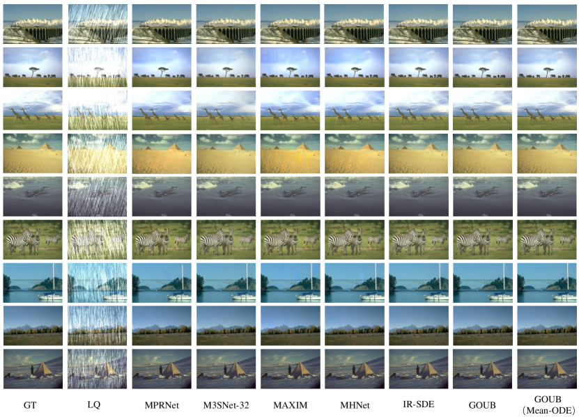
Figure 6: Additional visual results on Rain100H datasets.

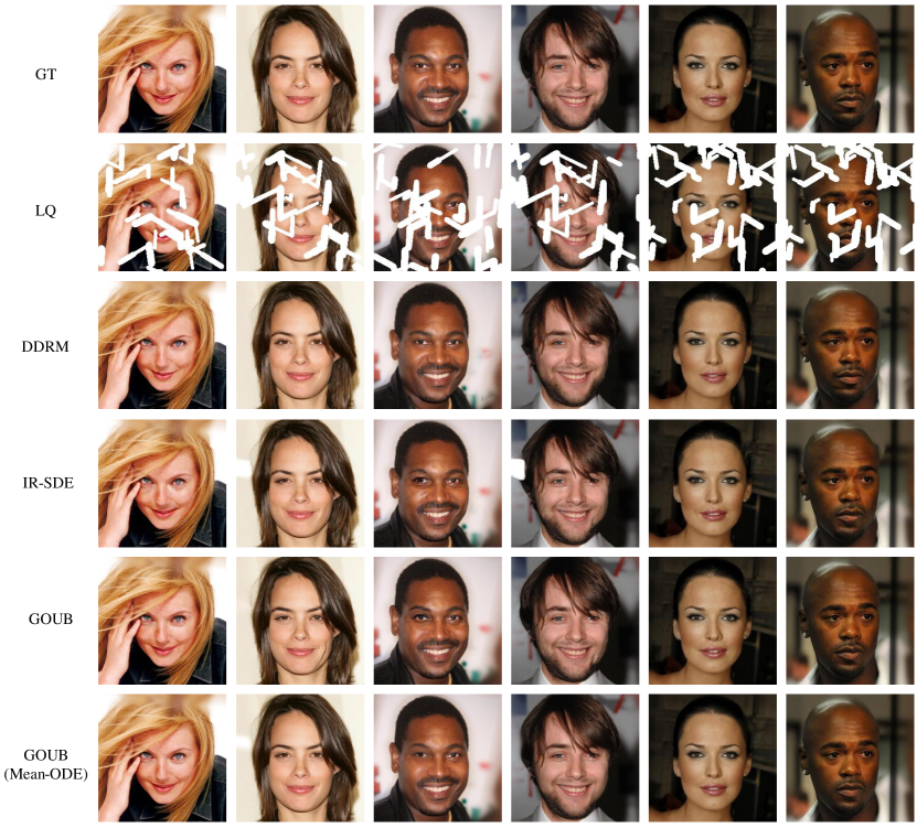
Figure 7: Additional visual results on CelebA-HQ datasets.

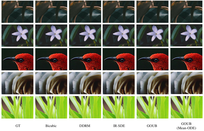
Figure 8: Additional visual results on DIV2K datasets.

References

- Banham and Katsaggelos (1997) Mark R Banham and Aggelos K Katsaggelos. Digital image restoration. IEEE signal processing magazine, 14(2):24–41, 1997.
- Zhou et al. (1988) Y-T Zhou, Rama Chellappa, Aseem Vaid, and B Keith Jenkins. Image restoration using a neural network. IEEE transactions on acoustics, speech, and signal processing, 36(7):1141–1151, 1988.
- Liang et al. (2021) Jingyun Liang, Jiezhang Cao, Guolei Sun, Kai Zhang, Luc Van Gool, and Radu Timofte. Swinir: Image restoration using swin transformer. In Proceedings of the IEEE/CVF international conference on computer vision, pages 1833–1844, 2021.
- Luo et al. (2023a) Ziwei Luo, Fredrik K Gustafsson, Zheng Zhao, Jens Sjölund, and Thomas B Schön. Refusion: Enabling large-size realistic image restoration with latent-space diffusion models. In Proceedings of the IEEE/CVF Conference on Computer Vision and Pattern Recognition, pages 1680–1691, 2023a.
- Zhang and Patel (2017) He Zhang and Vishal M Patel. Convolutional sparse and low-rank coding-based rain streak removal. In 2017 IEEE Winter conference on applications of computer vision (WACV), pages 1259–1267. IEEE, 2017.
- Yang et al. (2020) Wenhan Yang, Robby T Tan, Shiqi Wang, Yuming Fang, and Jiaying Liu. Single image deraining: From model-based to data-driven and beyond. IEEE Transactions on pattern analysis and machine intelligence, 43(11):4059–4077, 2020.
- Xiao et al. (2022) Jie Xiao, Xueyang Fu, Aiping Liu, Feng Wu, and Zheng-Jun Zha. Image de-raining transformer. IEEE Transactions on Pattern Analysis and Machine Intelligence, 2022.
- Zhang et al. (2018a) Kai Zhang, Wangmeng Zuo, and Lei Zhang. Ffdnet: Toward a fast and flexible solution for cnn-based image denoising. IEEE Transactions on Image Processing, 27(9):4608–4622, 2018a.
- Li et al. (2022) Boyun Li, Xiao Liu, Peng Hu, Zhongqin Wu, Jiancheng Lv, and Xi Peng. All-in-one image restoration for unknown corruption. In Proceedings of the IEEE/CVF Conference on Computer Vision and Pattern Recognition, pages 17452–17462, 2022.
- Soh and Cho (2022) Jae Woong Soh and Nam Ik Cho. Variational deep image restoration. IEEE Transactions on Image Processing, 31:4363–4376, 2022.
- Zhang et al. (2023a) Dan Zhang, Fangfang Zhou, Yuwen Jiang, and Zhengming Fu. Mm-bsn: Self-supervised image denoising for real-world with multi-mask based on blind-spot network. In Proceedings of the IEEE/CVF Conference on Computer Vision and Pattern Recognition, pages 4188–4197, 2023a.
- Yuan et al. (2007) Lu Yuan, Jian Sun, Long Quan, and Heung-Yeung Shum. Image deblurring with blurred/noisy image pairs. In ACM SIGGRAPH 2007 papers, pages 1–es. 2007.
- Kong et al. (2023) Lingshun Kong, Jiangxin Dong, Jianjun Ge, Mingqiang Li, and Jinshan Pan. Efficient frequency domain-based transformers for high-quality image deblurring. In Proceedings of the IEEE/CVF Conference on Computer Vision and Pattern Recognition, pages 5886–5895, 2023.
- Jain et al. (2023) Jitesh Jain, Yuqian Zhou, Ning Yu, and Humphrey Shi. Keys to better image inpainting: Structure and texture go hand in hand. In Proceedings of the IEEE/CVF Winter Conference on Applications of Computer Vision, pages 208–217, 2023.
- Zhang et al. (2023b) Guanhua Zhang, Jiabao Ji, Yang Zhang, Mo Yu, Tommi S Jaakkola, and Shiyu Chang. Towards coherent image inpainting using denoising diffusion implicit models. 2023b.
- Dong et al. (2015) Chao Dong, Chen Change Loy, Kaiming He, and Xiaoou Tang. Image super-resolution using deep convolutional networks. IEEE transactions on pattern analysis and machine intelligence, 38(2):295–307, 2015.
- Zamfir et al. (2023) Eduard Zamfir, Marcos V Conde, and Radu Timofte. Towards real-time 4k image super-resolution. In Proceedings of the IEEE/CVF Conference on Computer Vision and Pattern Recognition, pages 1522–1532, 2023.
- Sohl-Dickstein et al. (2015) Jascha Sohl-Dickstein, Eric Weiss, Niru Maheswaranathan, and Surya Ganguli. Deep unsupervised learning using nonequilibrium thermodynamics. In International conference on machine learning, pages 2256–2265. PMLR, 2015.
- Ho et al. (2020) Jonathan Ho, Ajay Jain, and Pieter Abbeel. Denoising diffusion probabilistic models. Advances in neural information processing systems, 33:6840–6851, 2020.
- Song and Ermon (2019) Yang Song and Stefano Ermon. Generative modeling by estimating gradients of the data distribution. Advances in neural information processing systems, 32, 2019.
- Song et al. (2020) Yang Song, Jascha Sohl-Dickstein, Diederik P Kingma, Abhishek Kumar, Stefano Ermon, and Ben Poole. Score-based generative modeling through stochastic differential equations. arXiv preprint arXiv:2011.13456, 2020.
- Karras et al. (2022) Tero Karras, Miika Aittala, Timo Aila, and Samuli Laine. Elucidating the design space of diffusion-based generative models. Advances in Neural Information Processing Systems, 35:26565–26577, 2022.
- Anderson (1982) Brian DO Anderson. Reverse-time diffusion equation models. Stochastic Processes and their Applications, 12(3):313–326, 1982.
- Dhariwal and Nichol (2021) Prafulla Dhariwal and Alexander Nichol. Diffusion models beat gans on image synthesis. Advances in neural information processing systems, 34:8780–8794, 2021.
- Ho and Salimans (2022) Jonathan Ho and Tim Salimans. Classifier-free diffusion guidance. arXiv preprint arXiv:2207.12598, 2022.
- Kawar et al. (2021) Bahjat Kawar, Gregory Vaksman, and Michael Elad. Snips: Solving noisy inverse problems stochastically. Advances in Neural Information Processing Systems, 34:21757–21769, 2021.
- Saharia et al. (2022) Chitwan Saharia, Jonathan Ho, William Chan, Tim Salimans, David J Fleet, and Mohammad Norouzi. Image super-resolution via iterative refinement. IEEE Transactions on Pattern Analysis and Machine Intelligence, 45(4):4713–4726, 2022.
- Kawar et al. (2022) Bahjat Kawar, Michael Elad, Stefano Ermon, and Jiaming Song. Denoising diffusion restoration models. Advances in Neural Information Processing Systems, 35:23593–23606, 2022.
- Chung et al. (2022a) Hyungjin Chung, Byeongsu Sim, Dohoon Ryu, and Jong Chul Ye. Improving diffusion models for inverse problems using manifold constraints. Advances in Neural Information Processing Systems, 35:25683–25696, 2022a.
- Chung et al. (2022b) Hyungjin Chung, Jeongsol Kim, Michael T Mccann, Marc L Klasky, and Jong Chul Ye. Diffusion posterior sampling for general noisy inverse problems. arXiv preprint arXiv:2209.14687, 2022b.
- Wang et al. (2023) Yinhuai Wang, Jiwen Yu, Runyi Yu, and Jian Zhang. Unlimited-size diffusion restoration. In Proceedings of the IEEE/CVF Conference on Computer Vision and Pattern Recognition, pages 1160–1167, 2023.
- Liu et al. (2022a) Guan-Horng Liu, Tianrong Chen, Oswin So, and Evangelos Theodorou. Deep generalized schrödinger bridge. Advances in Neural Information Processing Systems, 35:9374–9388, 2022a.
- De Bortoli et al. (2021) Valentin De Bortoli, James Thornton, Jeremy Heng, and Arnaud Doucet. Diffusion schrödinger bridge with applications to score-based generative modeling. Advances in Neural Information Processing Systems, 34:17695–17709, 2021.
- Su et al. (2022) Xuan Su, Jiaming Song, Chenlin Meng, and Stefano Ermon. Dual diffusion implicit bridges for image-to-image translation. arXiv preprint arXiv:2203.08382, 2022.
- Shi et al. (2023) Yuyang Shi, Valentin De Bortoli, Andrew Campbell, and Arnaud Doucet. Diffusion schrödinger bridge matching. arXiv preprint arXiv:2303.16852, 2023.
- Liu et al. (2023) Guan-Horng Liu, Arash Vahdat, De-An Huang, Evangelos A Theodorou, Weili Nie, and Anima Anandkumar. SB: Image-to-image schrödinger bridge. arXiv preprint arXiv:2302.05872, 2023.
- Li et al. (2023) Bo Li, Kaitao Xue, Bin Liu, and Yu-Kun Lai. Bbdm: Image-to-image translation with brownian bridge diffusion models. In Proceedings of the IEEE/CVF Conference on Computer Vision and Pattern Recognition, pages 1952–1961, 2023.
- Zhou et al. (2023) Linqi Zhou, Aaron Lou, Samar Khanna, and Stefano Ermon. Denoising diffusion bridge models. arXiv preprint arXiv:2309.16948, 2023.
- Vincent (2011) Pascal Vincent. A connection between score matching and denoising autoencoders. Neural computation, 23(7):1661–1674, 2011.
- Song et al. (2021) Yang Song, Conor Durkan, Iain Murray, and Stefano Ermon. Maximum likelihood training of score-based diffusion models. Advances in Neural Information Processing Systems, 34:1415–1428, 2021.
- Ahmad (1988) R Ahmad. Introduction to stochastic differential equations, 1988.
- Särkkä and Solin (2019) Simo Särkkä and Arno Solin. Applied stochastic differential equations, volume 10. Cambridge University Press, 2019.
- Luo et al. (2023b) Ziwei Luo, Fredrik K Gustafsson, Zheng Zhao, Jens Sjölund, and Thomas B Schön. Image restoration with mean-reverting stochastic differential equations. arXiv preprint arXiv:2301.11699, 2023b.
- Boyd and Vandenberghe (2004) Stephen P Boyd and Lieven Vandenberghe. Convex optimization. Cambridge university press, 2004.
- Hastie et al. (2009) Trevor Hastie, Robert Tibshirani, Jerome H Friedman, and Jerome H Friedman. The elements of statistical learning: data mining, inference, and prediction, volume 2. Springer, 2009.
- Wang et al. (2004) Zhou Wang, Alan C Bovik, Hamid R Sheikh, and Eero P Simoncelli. Image quality assessment: from error visibility to structural similarity. IEEE transactions on image processing, 13(4):600–612, 2004.
- Zhang et al. (2018b) Richard Zhang, Phillip Isola, Alexei A Efros, Eli Shechtman, and Oliver Wang. The unreasonable effectiveness of deep features as a perceptual metric. In Proceedings of the IEEE conference on computer vision and pattern recognition, pages 586–595, 2018b.
- Heusel et al. (2017) Martin Heusel, Hubert Ramsauer, Thomas Unterthiner, Bernhard Nessler, and Sepp Hochreiter. Gans trained by a two time-scale update rule converge to a local nash equilibrium. Advances in neural information processing systems, 30, 2017.
- Karras et al. (2017) Tero Karras, Timo Aila, Samuli Laine, and Jaakko Lehtinen. Progressive growing of gans for improved quality, stability, and variation. arXiv preprint arXiv:1710.10196, 2017.
- Potlapalli et al. (2023) Vaishnav Potlapalli, Syed Waqas Zamir, Salman Khan, and Fahad Shahbaz Khan. Promptir: Prompting for all-in-one blind image restoration. arXiv preprint arXiv:2306.13090, 2023.
- Yang et al. (2017) Wenhan Yang, Robby T Tan, Jiashi Feng, Jiaying Liu, Zongming Guo, and Shuicheng Yan. Deep joint rain detection and removal from a single image. In Proceedings of the IEEE conference on computer vision and pattern recognition, pages 1357–1366, 2017.
- Zamir et al. (2021) Syed Waqas Zamir, Aditya Arora, Salman Khan, Munawar Hayat, Fahad Shahbaz Khan, Ming-Hsuan Yang, and Ling Shao. Multi-stage progressive image restoration. In Proceedings of the IEEE/CVF conference on computer vision and pattern recognition, pages 14821–14831, 2021.
- Gao et al. (2023) Hu Gao, Jing Yang, Ying Zhang, Ning Wang, Jingfan Yang, and Depeng Dang. A mountain-shaped single-stage network for accurate image restoration. arXiv preprint arXiv:2305.05146, 2023.
- Tu et al. (2022) Zhengzhong Tu, Hossein Talebi, Han Zhang, Feng Yang, Peyman Milanfar, Alan Bovik, and Yinxiao Li. Maxim: Multi-axis mlp for image processing. In Proceedings of the IEEE/CVF Conference on Computer Vision and Pattern Recognition, pages 5769–5780, 2022.
- Gao and Dang (2023) Hu Gao and Depeng Dang. Mixed hierarchy network for image restoration. arXiv preprint arXiv:2302.09554, 2023.
- Agustsson and Timofte (2017) Eirikur Agustsson and Radu Timofte. Ntire 2017 challenge on single image super-resolution: Dataset and study. In Proceedings of the IEEE conference on computer vision and pattern recognition workshops, pages 126–135, 2017.
- Chung et al. (2023) Hyungjin Chung, Jeongsol Kim, Sehui Kim, and Jong Chul Ye. Parallel diffusion models of operator and image for blind inverse problems. In Proceedings of the IEEE/CVF Conference on Computer Vision and Pattern Recognition, pages 6059–6069, 2023.
- Zhao et al. (2023) Zixiang Zhao, Haowen Bai, Yuanzhi Zhu, Jiangshe Zhang, Shuang Xu, Yulun Zhang, Kai Zhang, Deyu Meng, Radu Timofte, and Luc Van Gool. Ddfm: denoising diffusion model for multi-modality image fusion. arXiv preprint arXiv:2303.06840, 2023.
- Murata et al. (2023) Naoki Murata, Koichi Saito, Chieh-Hsin Lai, Yuhta Takida, Toshimitsu Uesaka, Yuki Mitsufuji, and Stefano Ermon. Gibbsddrm: A partially collapsed gibbs sampler for solving blind inverse problems with denoising diffusion restoration. arXiv preprint arXiv:2301.12686, 2023.
- Feng et al. (2023) Berthy T Feng, Jamie Smith, Michael Rubinstein, Huiwen Chang, Katherine L Bouman, and William T Freeman. Score-based diffusion models as principled priors for inverse imaging. arXiv preprint arXiv:2304.11751, 2023.
- Lipman et al. (2022) Yaron Lipman, Ricky TQ Chen, Heli Ben-Hamu, Maximilian Nickel, and Matt Le. Flow matching for generative modeling. arXiv preprint arXiv:2210.02747, 2022.
- Liu et al. (2022b) Xingchao Liu, Chengyue Gong, and Qiang Liu. Flow straight and fast: Learning to generate and transfer data with rectified flow. arXiv preprint arXiv:2209.03003, 2022b.
- Tong et al. (2023) Alexander Tong, Nikolay Malkin, Kilian Fatras, Lazar Atanackovic, Yanlei Zhang, Guillaume Huguet, Guy Wolf, and Yoshua Bengio. Simulation-free schrödinger bridges via score and flow matching. arXiv preprint arXiv:2307.03672, 2023.
- Salminen (1984) P. Salminen. On conditional ornstein-uhlenbeck processes. Advances in Applied Probability, 16(4):920–922, 1984. ISSN 00018678. URL http://www.jstor.org/stable/1427347.
- Cheridito et al. (2003) Patrick Cheridito, Hideyuki Kawaguchi, and Makoto Maejima. Fractional ornstein-uhlenbeck processes. 2003.
- Heng et al. (2021) Jeremy Heng, Valentin De Bortoli, Arnaud Doucet, and James Thornton. Simulating diffusion bridges with score matching. arXiv preprint arXiv:2111.07243, 2021.
- Chow (2009) Winston C Chow. Brownian bridge. Wiley interdisciplinary reviews: computational statistics, 1(3):325–332, 2009.
- Risken and Risken (1996) Hannes Risken and Hannes Risken. Fokker-planck equation. Springer, 1996.
- Kingma and Ba (2014) Diederik P Kingma and Jimmy Ba. Adam: A method for stochastic optimization. arXiv preprint arXiv:1412.6980, 2014.
- Nichol and Dhariwal (2021) Alexander Quinn Nichol and Prafulla Dhariwal. Improved denoising diffusion probabilistic models. In International Conference on Machine Learning, pages 8162–8171. PMLR, 2021.