Integrated Qubit Reuse and Circuit Cutting for Large Quantum Circuit Evaluation

Abstract.

Quantum computing has recently emerged as a promising computing paradigm for many application domains. However, the size of quantum circuits that can run with high fidelity is constrained by the limited quantity and quality of physical qubits. Recently proposed schemes, such as wire cutting and qubit reuse, mitigate the problem but produce sub-optimal results as they address the problem individually. In addition, gate cutting, an alternative circuit-cutting strategy, has not been fully explored in the field.

In this paper, we propose IQRC, an integrated approach that exploits qubit reuse and circuit cutting (including wire cutting and gate cutting) to run large circuits on small quantum computers. Circuit-cutting techniques introduce non-negligible post-processing overhead, which increases exponentially with the number of cuts. IQRC exploits qubit reuse to find better cutting solutions to minimize the cut numbers and thus the post-processing overhead. Our evaluation results show that on average we reduce the number of cuts by 34% and additional reduction when considering gate cuts.

1. Introduction

Quantum computing has recently emerged as a promising computing paradigm for many application domains, such as machine learning (QNN, ; ML, ; ML2, ), chemistry simulation (chemistry, ; chem1, ; chem2, ), and optimization (optimization, ; finance_optimization, ). The problems from these domains scale quickly such that they require increasingly larger fault-tolerant quantum computers. Unfortunately, we are currently in the NISQ (noisy intermediate-scale quantum) era (Book, ) where quantum devices suffer from various noises, e.g., short coherence time and crosstalk among qubits, and small device sizes, e.g., current quantum devices only have up to 100s of qubits.

It has become one of the major challenges to run large quantum circuits in the NISQ era. Large quantum computers, e.g., IBM 433 osprey, often have limited availability to the general public. In addition, not all qubits of large quantum computers exhibit high computation fidelity — some noisy qubits have to be frozen, i.e., not used, for some computation tasks (frozen, ). Error mitigation schemes (error1, ; error2, ; error3, ; error4, ) help to improve computation fidelity (Book, ; hammer, ; QNN, ) but have limited effectiveness due to the limited availability of physical qubits on devices. As an alternative to physical quantum execution, software simulation offers a noise-free execution environment for quantum circuits. However, the simulation cost increases exponentially with the number of qubits (Large_Simulation, ) and thus faces intrinsic drawbacks for scalability.

Recently proposed schemes, i.e., wire cutting, qubit reuse, and gate cutting, help to mitigate the challenge. The wire-cutting schemes (cutqc, ; Peng, ; clifford_cutting, ) partition a large quantum circuit into several smaller subcircuits, run subcircuits on quantum devices, and then reconstruct the output of the original circuit through classical post-processing. That is, they adopt a hybrid approach that combines physical quantum execution and classical software post-processing. Since the classical post-processing overhead increases exponentially with the number of wire cuts, minimizing cut numbers is one of the major design goals in these schemes. The qubit-reuse technique (qubit_reuse, ; qubitreuse2, ; qubitreuse3, ) addresses the challenge by exploiting the hardware support for Mid-Circuit Measurement and Reset (MR) (mid-circuit, ) such that the physical qubits that have finished all their operations can be redeployed as other logical qubits during circuit execution. Another circuit-cutting approach, gate cutting (Mitarai_2021, ), was recently proposed to cut a two-qubit gate into a linear sum of single-qubit gates, and exploit classical post-processing to reconstruct the original result. Gate cutting has not been well-studied at the circuit level, i.e., deciding the best cut locations for a given large circuit.

Unfortunately, we observe that these schemes are currently applied individually and tend to produce sub-optimal results. Qubit reuse can reuse physical qubits only after their initially assigned operations finish. Its effectiveness diminishes as the circuits grow larger — only a few qubits can start their operations after some other qubits have finished. Wire cutting introduces one extra qubit (initialization qubit in (cutqc, )) after each cut, which may artificially increase the total number of physical qubits required for partitioning circuits. Gate cutting has not been well-studied at the circuit level. In addition, gate cutting, since its post-processing cannot reconstruct the distribution result, can only be applied to the quantum circuits that compute expectation values.

In this work, we present IQRC, a framework for evaluating larger quantum circuits on small quantum devices through integrated Qubit-Reuse and Circuit Cutting.IQRC is an end-to-end approach that models a large quantum circuit using ILP (integer linear programming), finds a good cutting solution using an ILP solver, maps the decision to subcircuits, runs the subcircuits on quantum devices, and reconstructs the original result through classical post-processing.

Compared with prior schemes, our key observation is that wire cuts in the circuit enlarge qubit-reuse opportunities, which in turn helps to eliminate unnecessary cuts in the circuit. By integrating qubit reuse and circuit cutting, IQRC strives to find better cutting solutions with fewer numbers of cuts, reduced post-processing overhead, and improved per-circuit computation fidelity. When only the quantum circuit’s expectation value is required, gate cutting enlarges the cutting possibilities and thus further decreases the number of required cuts. We summarize our contributions as follows.

• We propose IQRC, a framework for evaluating large circuits on small quantum computers. To the best of our knowledge, IQRC is the first framework that (i) integrates wire and gate cuttings; and (ii) exploits qubit reuse to take advantage of the opportunities from circuit cutting.

• We formulate the problem as a searching framework using ILP, which enables the searching for solutions under different optimization goals. The ILP formulation helps to achieve efficiency in an enlarged search space, and better scalability over the state-of-the-art (cutqc, ).

• We evaluate IQRC using different benchmarks. Our results show that, on average, we reduce the number of cuts by 34% when considering only wire cuts and additional reduction when considering wire and gate cuts. We verify our approach using real device execution and post-processing.

2. Background

2.1. Quantum Circuits and their Outputs

A quantum program is represented as a quantum circuit consisting of qubits and quantum gates. Current quantum hardware supports single-qubit and two-qubit gates, which are also the gates considered in this paper. A quantum circuit, represented as a unitary matrix $\mathcal{U}$, takes an initial qubit state —$\psi\rangle$, usually —0$\rangle$^⊗n, and evolves it to an output state —$\phi\rangle$.

(1) $$\mathcal{U}|\psi\rangle=|\phi\rangle$$

Given the superposition characteristic of quantum computation, the output state —$\phi\rangle$ is a probabilistic vector, that represents the probability distribution of measuring each of the possible 2ⁿ states. An alternative representation of a quantum state is density matrix representation, whereby the state —$\phi\rangle$ can be represented as the density matrix $\rho$ as

(2) $$\rho=|\phi\rangle\langle\phi|$$

An important characteristic of the output state is its expectation value which is calculated, in the computational measurement basis M, as

(3) $$\mathbf{E}=\langle\phi|M|\phi\rangle$$

Two Types of Quantum Output.

Many quantum algorithms, e.g., Grover’s algorithm for quantum search (grover1996fast, ), compute a probability vector as the output and use the vector to reflect the likelihood of each potential solution being the correct one. The probability vector is also important for quantum state analysis, sampling and statistics, and error analysis.

Other algorithms, e.g., Variational Quantum Algorithm (VQA) (error1, ; VQA2, ), use a hybrid quantum-classical approach to find the minimum of a cost function, which is often expressed as the expectation value of a Hamiltonian. The expectation value serves as feedback to adjust the parameters of the quantum circuit, aiming to find the optimal solution.

2.2. Quantum Circuit Simulation

Quantum circuits can be simulated on classical computers using state-vector simulation. The classical simulation provides an ideal noise-free run of quantum circuits and accurately reproduces the output. However, there is an exponential cost of simulation, which restricts the simulation of larger quantum circuits. Wu et al. showed that simulating the 61-qubit Grover search algorithm needed Argonne’s Theta supercomputer with 4,096 nodes and 768TB memory (Large_Simulation, ).

An alternative approach to simulation is to run the circuits on real quantum computers, using the shots-based model. That is, the quantum circuit is executed thousands of times, with each execution referred to as a shot, on the quantum hardware and the measurement of each qubit from each shot is summarized as the output probability-vector of the circuit. The drawbacks of this approach are: (i) many shots are required, even in an ideal noise-free setting, in order to accurately reproduce the output probability vector of the original circuit; (ii) given that today’s quantum computers are noisy, the computation fidelity is often low for large circuit execution; (iii) the available quantum computers have limited numbers of qubits. The largest quantum computer from IBM has 433 physical qubits (Osprey, ).

2.3. Circuit Cutting

Circuit cutting is a technique for obtaining the result of a large quantum circuit on small quantum devices. After cutting the large circuit into two or more smaller subcircuits using either wire cutting or gate cutting, circuit cutting can execute the subcircuits on quantum devices, and generate the result of the original circuit from the classical post-processing of the results of subcircuit executions (Peng, ). The post-processing overhead increases exponentially with the number of cuts, as we elaborate next.

2.3.1. Wire Cutting (W-Cut)

Wire cutting (W-Cut) (Peng, ; cutqc, ) cuts the quantum wire that connects two quantum gates, as shown in Figure LABEL:fig:methods(a). Here, U1 and U2 are two generic two-qubit gates. W-Cut cuts the original circuit into two independent subcircuits: subcircuit₀ and subcircuit₁, as shown in the figure. To obtain the output state $|\rho\rangle$ of the original circuit, CutQC (cutqc, ) runs subcircuit₀ with measurements in four bases, and subcircuit₁ with four initializations; and then reconstructs the output of the original circuit using Equation (4).

(4) $$\rho=\frac{A_{1}+A_{2}+A_{3}+A_{4}}{2}$$

where

$$A_{1} =Tr(\rho I)[|0\rangle\langle 0|+|1\rangle\langle 1|]$$

$$A_{2} =Tr(\rho Z)[|0\rangle\langle 0|-|1\rangle\langle 1|]$$

$$A_{3} =Tr(\rho X)[2|+\rangle\langle+|-|0\rangle\langle 0|-|1\rangle\langle 1|]$$

$$A_{4} =Tr(\rho Y)[2|i\rangle\langle i|-|0\rangle\langle 0|-|1\rangle\langle 1|]$$

Here, Tr() is the trace operator indicating running subcircuit₀ physically on quantum devices and measuring the output in one of the Pauli basis bases (i.e., M $\in${I, X, Y, Z}). Measuring a qubit in either the I or Z basis gives the same circuit. $|x\rangle\langle x|$ is the density matrix indicating initializing subcircuit₁ in one of the eigen states (i.e., I $\in${$|0\rangle$, $|1\rangle$, $|+\rangle$, $|i\rangle$}). From Equation 4, W-Cut needs four pairs of Kronecker products between the subcircuit results to reconstruct the result of the original circuit. If it takes $k$ ($k$¿0) cuts to partition a large circuit into multiple independent subcircuits, the classical post-processing overhead of result reconstruction is O(4^k).

Applying W-Cut at the circuit level is an optimization problem that finds the wires to be cut in a given large circuit such that the cutting has the smallest $k$ and ensures the execution of each subcircuit on small quantum devices. CutQC formulates the problem as an MIP (mixed integer programming) model and exploits an MIP solver to search for the best solution.

2.3.2. Gate Cutting (G-Cut)

Gate cutting (G-Cut) cuts a two-qubit quantum gate, e.g., $U3$ in Figure LABEL:fig:methods(b), into a linear sum of single-qubit gates $U_{3.T}$ and $U_{3.B}$. According to the theory of gate cutting (Mitarai_2021, ), if G-Cut cuts a two-qubit gate of the form $e^{i\theta A_{1}\otimes A_{2}}$ (e.g., CNOT, CZ, and ZZ gates) where A${}_{1}^{2}$ = A${}_{2}^{2}$ = I, the expectation value $\mathbf{E}$ of the original circuit can be reproduced based on the output state —$\phi_{i}\rangle$ of subcircuits, using Equation (5).

G-Cut produces six subcircuit instances, i.e., $\phi_{1}$ to $\phi_{6}$. Each $\phi_{i}$ is an independent instance, during its execution, we remove the two-qubit gate that has been cut from the original circuit, and replace it with single-qubit gates of the respective instance. The M${}_{A_{i}}$ term is single qubit measurement operations, with $\beta$ representing the outcome of the measurement, $\beta$ $\in$ {1,-1}. More details can be found in (Mitarai_2021, ).

G-Cut has not been well-studied at the circuit level. Given a large circuit, it remains an open problem to determine the subset of two-qubit gates to be cut for achieving our design goal, in particular, together with W-Cut and qubit reuse.

(5) $$\mathbf{E}[\phi]=\sum^{6}_{i=1}c_{i}E[\phi_{i}]$$

where,

$$\phi_{1} =\mathbf{S}(I\otimes I) c_{1}=cos^{2}(\theta)$$

$$\phi_{2} =\mathbf{S}(A_{1}\otimes A_{2}) c_{2}=sin^{2}(\theta)$$

$$\phi_{3} =\beta\mathbf{M}_{A_{1},\beta}\otimes\mathbf{S}(e^{i\pi A_{2}/4}) c_{3}=cos(\theta)sin(\theta)$$

$$\phi_{4} =\beta\mathbf{M}_{A_{1},\beta}\otimes\mathbf{S}(e^{-i\pi A_{2}/4}) c_{4}=-cos(\theta)sin(\theta)$$

$$\phi_{5} =\mathbf{S}(e^{i\pi A_{1}/4})\otimes\beta\mathbf{M}_{A_{2},\beta} c_{5}=cos(\theta)sin(\theta)$$

$$\phi_{6} =\mathbf{S}(e^{-i\pi A_{1}/4})\otimes\beta\mathbf{M}_{A_{2},\beta} c_{6}=-cos(\theta)sin(\theta)$$

2.4. Measure and Reset Functionality

IBM recently introduced mid-circuit measurement operation and mid-circuit reset operation (mid-circuit, ) to support dynamic circuits for quantum error correction(qec1, ; qec2, ; qec3, ) and runtime program verification(verification, ; verification2, ). As shown in Figure LABEL:fig:methods(c), once qubit q₀ finishes its operation with gate $U1$, we perform the measurement on this physical qubit, and re-initialize another logical qubit q₂ in the —0$\rangle$ state, and assign qubit q₂ to the same physical qubit on the quantum device. This is referred to as qubit-reuse in (qubit_reuse, ). In the figure, qubit-reuse enables the execution of the original three-qubit circuit on a two-qubit quantum device.

CaQR (qubit_reuse, ) proposes a compiler-assisted tool that automatically identifies qubit-reuse opportunities in a given circuit, reduces the total number of required physical qubits, and achieves better performance and computation fidelity. The effectiveness of qubit reuse diminishes as the circuit becomes bigger — only few qubits can delay their operations enough to start after some other qubits have finished.

3. Motivation

In this section, we use an example, as shown in Figure LABEL:fig:_Motivational_example, to demonstrate the effectiveness when integrating qubit reuse, wire cutting, and gate cutting together. Our problem is to run a 5-qubit quantum circuit on small quantum devices, e.g., 4-qubit or 3-qubit quantum devices.

When adopting CutQC (cutqc, ), the original circuit is split into two subcircuits using three cuts, as shown in Figure LABEL:fig:_Motivational_example(b). Each subcircuit has four qubits. Three extra qubits (i.e., the initialization qubits) are introduced, e.g., the first wire cut on $q2$ generates an extra qubit $q5$, which is now the second qubit in $subcircuit_{1}$. It leaves a measurement in $subcircuit_{0}$. We use three color pairs to indicate the introduced measurement operation and its matching initialization bit.

For this circuit, CutQC can’t find a solution that splits the original circuit into two 3-qubit subcircuits. It is also impossible to apply qubit reuse (qubit_reuse, ) directly on the original circuit to reduce the number of required qubits.

3.1. W-Cut and qubit-reuse

Figure LABEL:fig:_Motivational_example(c) shows the cutting result when we integrate W-Cut and qubit reuse. The integrated scheme, even though choosing the same cutting positions as those in CutQC, generates two 3-qubit subcircuits.

The improvement comes from the reuse opportunities exposed from wire cutting. For example, for $subcircuit_{0}$, qubit $q2$ becomes idle after the first cut. It can be reused by the initialization qubit. By exploiting the qubit reuse opportunities, each subcircuit requires one fewer qubit so that both can run on three-qubit quantum devices.

W-cut partitions the operations on the cut qubit, such that it introduces new qubit reuse opportunities into the circuit, which previously did not exist.

3.2. W-Cut and G-Cut

Figure LABEL:fig:_Motivational_example(c) shows the cutting result when we integrate W-Cut and G-Cut. The integrated scheme can cut the original circuit into two subcircuits in two cuts — one wire cut and one gate cut. The two-qubit gate $CZ$ is cut into two single-qubit gate instances $U_{T}$ and $U_{B}$ in different subcircuits.

For both W-Cut and G-Cut, their classical post-processing overheads increase exponentially to the number of cuts. However, G-Cut is slightly more expensive than W-Cut, i.e., O(4^k1) and O(6^k2) where $k1$ and $k2$ are the numbers of wire cuts and gate cuts, respectively. Consequently, for a cutting solution that has $k1$ wire cuts and $k2$ gate cuts, referred to as S($k1$,$k2$), its classical post-processing costs is O($4^{k1}6^{k2}$). We need to consider the cost difference when choosing a better-cutting solution. For example, while it is better to choose S(1,1) over S(2,1) (for the example in the figure), it is worse to choose S(0,4) over S(5,0).

4. The IQRC Framework

In this section, we elaborate IQRC, an end-to-end framework, for running a large quantum circuit on small quantum devices. Given a large circuit, IQRC converts it to a QR (qubit-reuse)-aware DAG, formulates it as an ILP model and sovles it, maps the cutting solutions to subcircuits, runs the subcircuits, and reconstructs the original result from post-processing.

4.1. The QR-aware DAG Representation

Given a $D$-qubit input quantum circuit that is to be cut for an $N$-bit quantum device ($D$¿$N$¿0), we first convert the circuit to a QR-aware DAG by adding dummy Identity gates such that, each qubit goes through the same number of quantum operations. After adding the identity gates, all qubits are aligned so that we define a quantum layer $m$ as the set of $m$-th gate for each qubit.

In Figure 3, V1, V6, and V7 are two-qubits gates, S2 and S4 are single-qubit gates, and F3, F5, F8, and F9 are inserted Identity gates. Gates S4, F5, and V6 belong to layer $M$. We place a yellow $\times$ on each wire before a gate to indicate a potential cutting location.

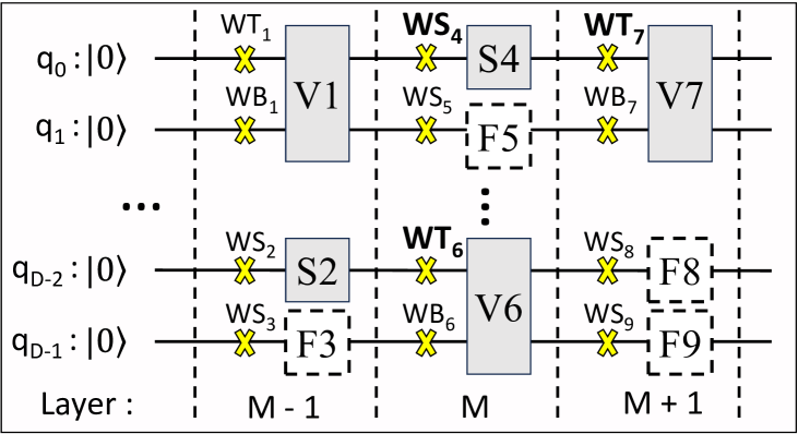
Figure 3. A QR-aware DAG representation of the quantum circuit.

Compared to the DAG for traditional wire cutting (cutqc, ) that lists two-qubit gates only, our QR-aware DAG explicitly lists all single-qubit gates and differentiates the cuts on the wires connecting different single qubits. For example, for the two cuts: (i) $WS_{4}$ is the one on the wire connecting the S4 gate and (ii) $WT_{7}$ is the one on the top wire connecting the V7 gate, the traditional DAG treats $WS_{4}$ and $WT_{7}$ as the same cut, as cutting at either location does not affect the number of required qubits in each subcircuit. However, when we consider qubit reuse, if there is another cut $WT_{6}$ (the top wire connecting V6), we may prefer to choose $WS_{4}$ if gate V1 and V6 are in the same subcircuit. This is because qubit $q_{0}$ can be reused for qubit $q_{D-2}$ while cutting at $WS_{4}$ disables this reuse. For discussion purposes, we assume the measurement and initialization operations take no depth and qubit-reuse does not increase circuit depth. Section 4.2.6 discusses how to handle the depths of these operations.

4.2. The ILP Model

4.2.1. The Meta Parameters

We formulate the problem as an ILP model. We first list the meta parameters, i.e., the constants that we define for the problem and/or we collect from preprocessing the input circuit.

• $D$ and $N$: They are the number of qubits in the input quantum circuit and the number of available physical qubits of the quantum device, respectively. We have $D$¿$N$¿0.

• $G_{max}$ and $W_{max}$: The maximum number of allowed gate cuts and wire cuts, respectively.

• $C_{min}$ and $C_{max}$: The minimum and maximum numbers of subcircuits to be cut, respectively. Note, our ILP solver often reports a cutting solution that has fewer than $C_{max}$ subcircuits. This is because our model focuses on reducing the classical post-processing cost, which does not relate to the number of subcircuits. As we elaborate next, the cost relates to a combination of wire cuts and gate cuts, as the two types of cuts have slightly different classical post-processing costs.

  If $C_{min}$=$C_{max}$, the solution that we find has the specified number of subcircuits.

• $\delta$: The relative weight for adjusting the optimization goal between classical post-processing overhead and computation fidelity. We will elaborate in Section 4.2.5.

• $G$-$Cut$-$enabled$: This is a binary parameter indicating if gate cutting should be enabled. As we discussed, after G-Cut, we can only reconstruct the expectation value of the circuit. If the original circuit is to compute the probability vector, we disable the gate cutting in the model.

4.2.2. ILP Variables

When preprocessing the original circuit, we differentiate three types of gates, i.e., two-qubit gates, single-qubit gates in the original circuit, and identity gates that we inserted. We number all gates and define a binary variable for each of the gates as follows.

$$V_{x,c} = \begin{cases}1&\text{if two-qubit gate $x$ is in subcircuit $c$}\\ 0&\text{Otherwise}\end{cases}$$

(6) $$S_{x,c} = \begin{cases}1&\text{if single-qubit gate $x$ is in subcircuit $c$}\\ 0&\text{Otherwise}\end{cases}$$

$$F_{x,c} = \begin{cases}1&\text{if identity gate $x$ is in subcircuit $c$}\\ 0&\text{Otherwise}\end{cases}$$

For single-qubit and identity gates, we can only perform W-Cut. We set the cutting point on the wire before each gate. We do not W-Cut any gate on the first layer.

(7) $$WS_{x}=\begin{cases}1&\text{if single-qubit/identity gate $x$ is W-Cut,}\\ 0&\text{Otherwise}\end{cases}$$

For two-qubit gates, we can perform both W-Cut and G-Cut. For W-Cut, we can cut either of its input wires but not both. We define the following variables.

$$U_{x} = \begin{cases}1&\text{if two-qubit gate x is neither W-Cut nor G-Cut}\\ 0&\text{Otherwise}\end{cases}$$

(8) $$WT_{x} = \begin{cases}1&\text{if top wire to two-qubit gate $x$ is W-Cut}\\ 0&\text{Otherwise}\end{cases}$$

$$WB_{x} = \begin{cases}1&\text{if bottom wire to two-qubit gate $x$ is W-Cut}\\ 0&\text{Otherwise}\end{cases}$$

$$G_{x} = \begin{cases}1&\text{if two-qubit gate x is G-Cut}\\ 0&\text{Otherwise}\end{cases}$$

When G-Cutting a two-qubit gate $x$, we get two single-qubit gates, referred to as $x.top$ and $x.bottom$. These two gates appear only if $G_{x}$=1. Similar to those in definition (6), we define variables to determine if they are in some subcircuits.

(9) $$GT_{x,c} = \begin{cases}1&\text{if for two-qubit gate $x$, we have }\\ &\text{$G_{x}$=1 and $x.top$ is in subcircuit c}\\ 0&\text{Otherwise}\end{cases}$$

$$GB_{x,c} = \begin{cases}1&\text{if for two-qubit gate $x$, we have }\\ &\text{$G_{x}$=1 and $x.bottom$ is in subcircuit c}\\ 0&\text{Otherwise}\end{cases}$$

4.2.3. The General ILP Constraints

We next list the general constraints in our model. These constraints are the same regardless of the input circuit and user parameters.

Whether a single-qubit or identity gate $x$ is cut is determined by its $WS_{x}$ variable. However, for a two-qubit gate, it may be W-Cut, G-Cut, or not cut. That is, we can W-Cut and G-Cut the gate at the same time. If it is W-Cut, we can only cut one of its input wires. Therefore, we have the following constraints for each two-qubit gate $x$.

$$U_{x}+WT_{x}+WB_{x}+G_{x} \geq 1$$

$$U_{x}+WT_{x} \leq 1$$

(10) $$U_{x}+WB_{x} \leq 1$$

$$U_{x}+G_{x} \leq 1$$

Each gate $x$ must belong to one and only one subcircuit, unless it is a two-qubit gate and has been G-Cut. If a two-qubit gate $x$ is G-Cut, its two-qubit gate form $conceptually$ disappears such that the two single-qubit gates, i.e., $x.top$ and $x.bottom$, emerge in the circuit. In this case, the newly generated single-qubit gates, i.e., $x.top$ and $x.bottom$, must belong to one and only one subcircuit. These two single-qubit gates cannot belong to the same subcircuit.

We use this technique to linearize the gate cut constraints. This technique is also used in Section 4.2.6.

$$\text{for single-qubit gate $x$, }\sum_{c\in C}S_{x,c} = 1$$

(11) $$\text{for two-qubit gate $x$, }\sum_{c\in C}V_{x,c}+G_{x} = 1$$

$$\sum_{c\in C}GT_{x,c} = G_{x}$$

$$\sum_{c\in C}GB_{x,c} = G_{x}$$

$$\text{for $\forall$ subcircuit $c\in C$,~{}~{}~{}~{}~{}}GT_{x,c}+GB_{x,c} \leq 1$$

After cutting, each subcircuit should not have more than $N$ qubits, i.e., the device size constraint. Therefore, for all identity gates $x$, single-qubit gates $s$, and two-qubit gates $t$, respectively at each layer $l$,

(12) $$Q_{c,l}=\sum_{x}F_{x,c}+\sum_{s}S_{s,c}+\sum_{t}(2V_{t,c}+GT_{t,c}+GB_{t,c})\leq N$$

where $Q_{c,l}$ is the number of qubits used in subcircuit $c$ at layer $l$. By adopting the layer-based cutting approach, our model allows us to find better qubit reuse opportunities such that a wire cut at an early layer can be reused by a different qubit at a later layer.

We also restrict the number of gate cuts and wire cuts.

$$\sum_{x}G_{x} \leq G_{max}$$

(13) $$\sum_{x}(WS_{x}+WT_{x}+WB_{x}) \leq W_{max}$$

4.2.4. The Circuit-dependent Constraints

In addition to the general constraints, we have circuit-dependent constraints. These constraints specify the relationship between two neighboring gates.

If two neighboring gates are two two-qubit gates, we may have two cases: (a) the bottom output of the upstream gate connects to the top input of the downstream gate, e.g, the U1-U3 connection in Figure LABEL:fig:methods(b); or (b) the top output of the upstream gate connects to the bottom input of the downstream gate, e.g, the U2-U3 connection. We specify their constraints as follows.

$$2\times WT_{U3} =\sum_{c\in C}(|V_{U1,c}-V_{U3,c}+GB_{U1,c}-GT_{U3,c}|)$$

(14) $$2\times WB_{U3} =\sum_{c\in C}(|V_{U2,c}-V_{U3,c}+GT_{U2,c}-GB_{U3,c}|)$$

If two neighboring gates are one upstream sing-qubit gate and one downstream two-qubit gate, for example, if we replace $U1$ and $U3$ with single-qubit gates, the constraints are

$$2\times WT_{U3} =\sum_{c\in C}(|S_{U1,c}-V_{U3,c}-GT_{U3,c}|)$$

(15) $$2\times WB_{U3} =\sum_{c\in C}(|S_{U2,c}-V_{U3,c}-GB_{U3,c}|)$$

Similar constraints are specified for other circuit connections. They follow the same rules of gate and wire cuts.

4.2.5. The Objective Function

Our ILP model consists of two optimization goals.

• Our main optimization goal is to minimize the classical post-processing overhead. Since each W-Cut and G-Cut require four and six products, respectively, the overhead is O(4^k6^t) for a cutting solution ($k$,$m$) having $k$ wire cuts and $m$ gate cuts.

  A naive integration of this cost in the objective function would lead to a non-linear component, which can greatly slow down the solver. Instead, we linearize the cost as $\alpha k+\beta m$ such that if the exponential cost of ($k_{1}$,$m_{1}$) is smaller than that of ($k_{2}$,$m_{2}$), our linear cost has the same relative relationship. In this work, we choose $\alpha$=3.25 and $\beta$=4.2 as they satisfy the requirement for the number of cuts smaller than 240 (120 W-cut and 120 G-cut).

  Therefore, the classical post-processing cost is

  (16) $$PPCost=\alpha\times\sum_{x}(WS_{x}+WT_{x}+WB_{x})+\beta\times\sum_{x}G_{x}$$

• The other optimization goal of our model is to improve the computation fidelity. Studies have shown that the computation error of a quantum circuit depends on the number of its operations, in particular, two-qubit quantum operations (gate-error1, ; gate-error-2, ; gate-error-3, ). This is because the error rate of two-qubit gates is orders of magnitude higher than that of single-qubit gates. To improve the computational fidelity after circuit cutting, we strive to balance the number of two-qubit gates across different subcircuits.

  We define a new variable $TE$ to track the maximal number of two-qubit gates in a subcircuit. Minimizing $TE$ would help to improve the overall computation fidelity. We add one linear constraint for each subcircuit $c$ as follows. This helps to find the subcircuit that has the maximal number of two-qubit gates.

  (17) $$TE \geq\sum_{x}V_{x,c}$$

  We further define the two-qubit gate related error as

  (18) $$CError=f(TE)$$

  Here, we choose a linear function to make sure $PPCost$ and $CError$ are at about the same value range. We use an example to explain how to choose the function. We first run the model considering $PPCost$ only such that we may find a cutting solution (4, 6) with the PPCost value being 3.25$\times$4+4.2$\times$6=38, the number of subcircuits being 5, and the current TE being 40. Assuming we can achieve a perfect balancing of the subcircuits with a maximal increase of 4 additional cuts and get a solution (6,7) with $PPcost$ being 53. The PPCost range is [38,53]. The TE range is now [20,40]. We a choose linear function $f$(TE)= TE$\times$0.75+23.

  Note, a further refined linear function can be derived for a given circuit.

Oftentimes, balancing the number of two-qubit gates across subcircuits may result in a cutting solution with more cuts and thus higher classical post-processing overhead, or even no solution. Therefore, we introduce another meta parameter $\delta$ to adjust the optimization goal between $PPCost$ and $CError$. The $\delta$ value can be integrated in deciding the linear function in $CError$.

To summarize, our objective function is as follows.

(19) $$\textbf{Min}[\delta\times PPCost+(1-\delta)\times CError]$$

4.2.6. Discussion

We make two simplifications for clarity purposes in the preceding discussion of the model. (1) We assume adding $Identity$ gates to ensure all layers have $D$ gates. This may introduce a large number of identity gates and their corresponding constraints, which slow down the solver. In our implementation, for a long wire that connects two gates far away from each other, we selectively add two or three identity gates at the beginning, middle, and end of the wire. (2) We assume the measurement and initialization operations take no depth. However, when considering their depths, we introduce a trailing measurement gate after the cut point, and a leading initialization gate before the cut point. These two gates emerge in the circuits only if the corresponding wire is cut. We use the same technique as that for gate cutting, i.e., only if a two-qubit gate is cut, its corresponding single-qubit gates emerge in the circuit.

4.3. Output Reconstruction

Reconstruction after W-Cut.

The original quantum circuit, if computing the probability distribution vector, can only be wire-cut. The probability vector results from subcircuit runs can be reconstructed using Equation (4). The classical postprocessing process follows the techniques as elaborated in CutQC (cutqc, ).

Reconstruction after W-Cut and G-Cut.

The original quantum circuit, if computing the expectation value, can be cut by both W-Cut and G-Cut. The reconstruction overhead of expectation values is lower than that of probability vectors as the expectation value is a floating point value, while a probability vector consists of multiple floating point values.

To reconstruct the expectation value of the original circuit, we sort the subcircuits according to the numbers of their qubits, and then start from the smallest subcircuit. For each subcircuit, we first reconstruct at the wire-cutting positions and then at the gate-cutting positions. When handling the W-Cut wires, we reconstruct the expectation values directly, instead of the probability vectors. The Equation (20) in Section 2 is applicable for both probability vectors and expectation values (Peng, ). For the latter, it can be adapted as follows.

(20) $$\mathbf{E}[\rho]=\frac{A_{1}+A_{2}+A_{3}+A_{4}}{2}$$

where

$$A_{1} =\mathbf{E}[Tr(\rho I)](\mathbf{E}[|0\rangle\langle 0|]+\mathbf{E}[|1\rangle\langle 1|])$$

$$A_{2} =\mathbf{E}[Tr(\rho Z)](\mathbf{E}[|0\rangle\langle 0|]-\mathbf{E}[|1\rangle\langle 1|])$$

$$A_{3} =\mathbf{E}[Tr(\rho X)](2\mathbf{E}[|+\rangle\langle+|]-\mathbf{E}[|0\rangle\langle 0|]-\mathbf{E}[|1\rangle\langle 1|])$$

$$A_{4} =\mathbf{E}[Tr(\rho Y)](2\mathbf{E}[|i\rangle\langle i|]-\mathbf{E}[|0\rangle\langle 0|]-\mathbf{E}[|1\rangle\langle 1|])$$

After the reconstruction from W-Cut, we adopt Equation (5) to handle G-Cut for reconstructing the expectation value of the original circuit.

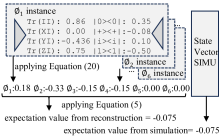
Figure 4. The reconstruction of the expectation value after W-Cut and G-Cut.

An example.

We next illustrate the reconstruction process for the example shown in Figure LABEL:fig:_Motivational_example(d). The original quantum circuit was cut into two subcircuits with one wire cut and one gate cut on a CZ gate. The CZ gate has the form

(21) $$CZ=e^{\frac{i\pi I\otimes Z}{4}}e^{\frac{i\pi Z\otimes I}{4}}e^{\frac{i\pi Z\otimes Z}{4}}$$

Each exponential term in this form can be decomposed as shown in Equation (5). We can then combine and simplify all three terms to the following six instances (Mitarai_2021, ). These instances are independent of each other.

$$\phi_{1} =\mathbf{S}(rz(\frac{-\pi}{2})\otimes rz(\frac{-\pi}{2})) c_{1}=\frac{1}{2}$$

$$\phi_{2} =\mathbf{S}(rz(\frac{\pi}{2})\otimes rz(\frac{\pi}{2})) c_{2}=\frac{1}{2}$$

$$\phi_{3} =\beta\mathbf{M}_{Z,\beta}\otimes\mathbf{S}(e^{i\pi Z/2}) c_{3}=\frac{-1}{2}$$

$$\phi_{4} =\beta\mathbf{M}_{Z,\beta}\otimes\mathbf{S}(I) c_{4}=\frac{1}{2}$$

$$\phi_{5} =\mathbf{S}(e^{i\pi Z/2})\otimes\beta\mathbf{M}_{Z,\beta} c_{5}=\frac{1}{2}$$

$$\phi_{6} =\mathbf{S}(I)\otimes\beta\mathbf{M}_{Z,\beta} c_{6}=\frac{-1}{2}$$

For example, during $\phi_{1}$ instance’s execution, we replace the two-qubit CZ gate with two single-qubit $rz(\frac{-\pi}{2})$ gates. We then reconstruct the expectation value of this instance, for the wire cut (whose reconstruction follows Equation (20)). Figure 4 shows the reconstructed expectation value of each $\phi_{i}$ (1$\leq$i$\leq$6) using Equation (20) and then the expectation value of the original circuit using Equation (5). For verification purposes, the expectation value of the original circuit is also computed through state vector simulation, which shows the same result.

5. Experimental Methodology

We evaluate the effectiveness of IQRC using different benchmarks and compare the results with those from CutQC (cutqc, ), the state-of-the-art wire-cutting scheme. While both were implemented using the Gurobi optimizer(gurobi, ), IQRC builds an ILP (integer linear programming) model while CutQC builds an MIP (mixed integer programming) model. In the experiments, we set the maximal number of cuts to 100. The imbalance threshold is set as 500 gates for CutQC. For the meta parameter $\delta$ in our scheme, we choose two values for case study purposes. A more appropriate value can be preset based on the noise model of the physical quantum device.

• IQRC-C: we choose $\delta$=1, i.e., we do not optimize the computation fidelity from balancing two-qubit gates across subcircuits. The subcircuits, due to their smaller sizes, generally have better computation fidelity than that of the original circuit. However, some subcircuits may have significantly better computation fidelity than others if they contain fewer two-qubit gates.

• IQRC-B: we choose $\delta$=3/4 such that the maximal value of $PPCost$ is roughly three times the maximal value of $CError$, as we discussed in Section 4.2.5. This case study is to evaluate the effectiveness if, in addition to the main design goal of reducing the post-processing overhead, we also balance the two-qubit gates for computation fidelity improvement.

We also run experiments on the IBM Lagos quantum computer through the IBM cloud service to verify our approach.

Table 1. Comparing W-Cut results using IQRC and CutQC. ( D and N are meta parameters in Section 4.2.1; #SC: the number of subcircuits after cutting; #Cuts: the number of wire cuts; #MS: the maximal number of two-qubit gates in the subcircuits)

Benchmark			CutQC			IQRC-C			IQRC-B
	D	N	#SC	#Cuts	#MS	#SC	#Cuts	#MS	#SC	#Cuts	#MS
QFT	15	7	No Solution			3	20	69	3	20	68
	15	9	9	44	27	2	12	81	2	12	75
	30	16	No Solution			2	28	330	2	28	318
	30	20	No Solution			2	20	380	2	20	335
	30	24	4	52	276	2	12	414	2	12	399
						4	14	413	4	32	145
	30	27	3	32	351	2	6	429	2	6	426
						3	7	428	3	30	146
SPM	15	7	3	6	8	3	5	9	3	6	8
	20	7	5	11	8	4	9	13	4	9	9
	30	16	3	8	22	2	6	25	2	6	25
	40	16	3	10	21	3	9	27	3	9	25
ADD	16	7	4	6	35	3	4	51	3	4	51
	22	7	5	8	34	4	6	51	4	6	51
	30	16	2	2	120	2	2	120	2	2	120
	40	16	4	16	74	4	16	75	5	16	71

5.1. Benchmarks

We test our scheme using two groups of benchmarks: one computes the probability distribution while the other computes the expectation value. We generate multiple quantum circuits for each benchmark. We use a three-letter abbreviation to indicate each benchmark, the abbreviation is in the parameters as we describe each benchmark next.

The following three benchmarks compute the probability distribution and thus can only be cut using W-Cut.

• QFT (QFT): Quantum Fourier Transform (qft, ) is an important building block in many quantum algorithms, including the Shor’s factoring algorithm.

• Supremacy (SPM): This is a type of random circuit that was used by Google to demonstrate quantum supremacy (Supremacy, ).

• Adder (ADD): This is a linear Ripple Carry Adder (adder, ), which reduces the number of ancilla qubits required to 1.

We also choose the Quantum Approximate Optimization Algorithm (qaoa, ) in the evaluation. Since it computes the expectation value, the quantum circuit can be cut using both W-Cut and G-Cut. We create three different testing graphs.

• m-Regular (REG): The graph in REG is a regular graph in which each node has $m$ edges (n-regular, ). By default, $m$=3.

• Erdos-Renyi (ERD): The graph in ERD is a random graph in which we exploit a probability $p$ in creating edges across different nodes in the graph (erdos, ). By default, $p$=0.1.

• Barabasi-Albert (BAR): The graph for this benchmark is also a random graph. Each node in the graph has $m$ edges that connect preferentially to nodes with high degrees (bara, ). by default, $m$=3.

6. Experimental Results

6.1. Wire Cutting Evaluation

Table 1 compares the results when we adopt three cutting schemes on the benchmarks that compute probability vectors. We report the number of subcircuits (#SC), the required number of cuts (#Cuts), and the maximal number of two-qubit gates in the subcircuits (#MS). CutQC cannot find solutions for some settings, which are reported as no-solution in the table. For the settings that IQRC finds a solution with a smaller #Cuts, e.g., QFT(D=30, N=24), we also report the solution with the same #Cuts from CutQC so that we can compare #MS.

From the table, our scheme significantly reduces the number of cuts — on average, IQRC-C and IQRC-B achieve 34% and 32% reductions over CutQC, respectively. The test cases from QFT have the most complicated circuits, i.e., the circuit in each setting has a large number of two-qubit gates that exhibit all-to-all connections among qubits. For these test cases, CutQC may not be able to find a solution if the device size $N$ is small. IQRC achieves the largest improvements in these settings. For example, IQRC reduces the #Cuts from 32 to 6 when D=30 and N=27, exhibiting 81% improvement.

When considering computation fidelity, our scheme helps to balance the two-qubit gates across subcircuits. For example, when comparing the solutions between IQRC-B and IQRC-C, the latter has smaller #MS values, indicating improved computation fidelity. For QFT(D=30, N=27), IQRC has larger #MS values than those of CutQC. This is because the solutions from IQRC have fewer subcircuits. When having the same number of subcircuits, IQRC-B achieves a significantly smaller #MS value, i.e., 146 vs 351.

6.2. Wire- and Gate- Cutting Evaluation

Table 2 compares the cutting solutions when applying cutting on the benchmarks that compute expectation values. We compare two choices for our scheme: one is to choose W-Cut only while the other allows both W-Cut and G-Cut.

For comparison purposes, if IQRC (both) has a solution ($k_{1}$, $k_{2}$), where $k_{1}$ and $k_{2}$ are the wire cut and gate cut numbers, respectively, its overhead 4${}^{k_{1}}$6${}^{k_{2}}$ is converted to 4${}^{k_{3}}$ with $k_{3}$ being the effective wire-cut number reported in the table. On average, IQRC (W-Cut only) and IQRC (both) achieve 25% and 28% reductions on the number of cuts. Exploiting G-Cut helps to further reduce post-processing overhead. For example, for ERD-50, IQRC (both) has an #EffCuts of 22.46. While being a small reduction over 24, it corresponds to 8.45$\times$ reduction in post-processing overhead compared to that of IQRC (W-Cut only).

Table 2. Comparison of W-Cut and W-Cut+G-Cut schemes (#EffCuts is the effective wire-cuts for comparison).

Benchmark			CutQC			IQRC-C (W-Cut Only)			IQRC-C (W-Cut and G-Cut)
	D	N	#SC	#Cuts	#MS	#SC	#Cuts	#MS	#SC	#W-cuts	#G-cuts	#EffCuts	#MS
REG	40	27	3	21	49	2	17	51	2	15	1	16.29	55
	46	27	3	32	48	2	20	58	2	17	2	19.58	58
	50	27	4	38	43	2	24	63	2	22	1	23.29	62
ERD	40	27	3	31	67	2	23	109	2	21	1	22.29	109
	45	27	3	26	54	2	20	58	2	14	4	19.17	63
	50	27	5	39	41	2	24	69	2	17	5	23.46	65
BAR	40	27	3	17	71	2	15	55	2	13	1	14.29	56
	45	27	3	23	71	2	19	70	2	17	1	18.29	72
	50	27	3	28	62	2	24	71	2	20	2	22.46	71

6.3. Real Machine Evaluation

We verify our approach by testing benchmark REG($m$=2) on the IBM 7-qubit LAGOS quantum computer. The computer has 1.7 physical connections per qubit. When we ran the experiments, it had median error rates of 8.25e^-3 for CNOT gates and 2.6e^-4 for single-qubit/$\sqrt{x}$ gates, respectively.

We choose $D$=7 and $N$=4, i.e., the original quantum circuit has seven qubits and IQRC partitions it into smaller circuits so that each subcircuit can run on a 4-qubit quantum computer. Table 3 compares four execution modes.

• State Vector Simulation: The result from the state vector simulation computes the ground truth for the comparison of the results from different schemes.

• Shot-based Simulation: In this mode, we run shot-based state-vector simulation, which uses the state-vector probability to introduce a random bit-string output every shot for simulating an ideal device. We report the average from 10 circuit runs with each run having 16,384 shots.

• Device Execution (7-qubit): We ran the 7-qubit original circuit on the real quantum computer with 16,384 shots for each run. We run 10 times and report the average.

• IQRC: IQRC partitions the original circuit into two subcircuits with one gate cut and one wire cut. The subcircuits are run with different measurement and initialization instances, resulting in a total of 42 instances. Each instance runs just one time (with 16,384 shots) using four physical qubits-qubit. The results from subcircuits are then combined to compute the result for the original circuit.

Table 3. Comparison between 7-qubit device execution and IQRC (4-qubit device execution + post-processing).

Execution Mode	Results	Accuracy
State Vector simulation	-0.0349	100$\%$
Shot-based Simulation	-0.0323	92$\%$
Device Execution (7-qubit)	-0.0078	22.3$\%$
IQRC-B	-0.0355	98.3%

From the table, IQRC achieves better accuracy than that of 7-qubit device execution. This is because (1) The original circuit has 16 two-qubit CNOT gates (and 9 of them were introduced from SWAP operation) while each of our subcircuits contains 3 CNOT gates. This results in better computation fidelity for the subcircuit execution. (2) the subcircuits have fewer qubits and short execution depths. Due to noisy qubits, the expectation value result from quantum device execution shows low accuracy, similar results were also observed in recent studies (hammer, ).

In addition, IQRC achieves better accuracy than that of shot-based simulation. The state vector of the shot-based simulation is 8$\times$ that of the 4-qubit device execution, which tends to introduce more randomness in output probability distribution than that of the real execution.

6.4. Time Comparison

In this section, we compare the time required to find the cutting solutions using IQRC and CutQC. For a fair comparison, we assume we know $k$, the number of subcircuits of the solution for each setting. This is because IQRC and CutQC work slightly differently. For IQRC, the user specifies a range [$C_{min}$,$C_{max}$] and the subcircuit number of the found solution $k$ is guaranteed to be within the range. For CutQC, the user needs to specify the exact $k$ such that CutQC searches for the best solution with $k$ subcircuits. For the latter, the user needs to manually increment $k$ if a smaller $k$ value results in $no$-$solution$. In the experiment, assuming we know $k$, we set $C_{min}$=$k$=$C_{max}$ for IQRC and start with $k$ for CutQC.

Table 4. Comparison of the time required to find out the cutting solutions using CutQC and IQRC.

Benchmark			CutQC	IQRC	Improvement
Name	D	N	time(s)	time(s)
SPM	20	7	11.7	6.21	47%
ADD	22	7	148.5	19.7	87%
QFT	30	27	1800	1.92	100%

Table 4 summarizes the wall clock time to find the solutions in Table 1. From the table, IQRC runs much faster than CutQC for most cases. On average, IQRC is 78% faster than CutQC. The main reason is that IQRC builds a linear model while CutQC adopts a non-linear model. The quadratic constraints in the CutQC model significantly slow down the solver in searching for the best cutting solution. In addition, without qubit reuse, CutQC introduces one extra qubit (i.e.,initialization qubit) after each cut, which increases the number of qubits in the subcircuit and makes it difficult to find a valid cutting solution.

6.5. Scalability

We next investigate the scalability of our ILP model, i.e., its ability to handle large and complicated quantum circuits. We observe that the difficulty of the cutting problem depends on two factors: (i) the $D$ and $N$ values. The problem becomes more difficult if we have a larger $D$ and a smaller $N$. (ii) the number of two-qubit gates in the original circuit. The more such gates the circuit has, the harder the problem is.

Table 5. The problem difficulty scales with circuit size and circuit complexity.

Benchmark			IQRC		CutQC
name	D	N	#W-Cuts	#G-Cuts	#W-Cuts
REG (m=3)	200	150	19	0	21
REG (m=3)	300	200	31	3	36
BAR (m=4)	200	150	74	3	No Solution
BAR (m=2)	300	200	55	1	60
ERD ($p$=0.05)	200	150	96	2	No Solution
ERD ($p$=0.02)	300	200	52	104	No Solution

We set both $D$ and $N$ to be bigger than 100, representing the problems that we target to solve in the NISQ era. We summarize our experimental results in Table 5. In the table, the tagged rows indicate that CutQC cannot find the solutions. For simple quantum problems, e.g., REG (m=3), scaling the $D$ and $N$ values does not increase problem complexity. The solver can quickly find such solutions. For the same quantum problem, e.g., BAR, if we have more two-qubit gates(i.e., choosing m=4 instead m=2) the problem becomes harder even if we have fewer qubits in the original circuit. For difficult quantum problems, e.g., ERD, choosing $D$=300, $N$=200, and $p$=0.02, our model scales well and finds the solution. However, the solution contains large numbers of wire cuts and gate cuts, indicating that bottleneck has shifted to the post-processing overhead, i.e., O(4⁵²6¹⁰⁴).

6.6. Qubit Reuse in Cutting

Based on the observation that IQRC exploits qubit reuse to find better cutting solutions than those of CutQC, it becomes interesting to investigate if naively combining CutQC and qubit reuse can achieve similar results.

To partition a $D$-qubit original circuit into smaller subcircuits that can run on $N$-qubit quantum devices, we have two simple approaches to combine CutQC and qubit reuse.

• For the first approach, we apply CutQC to partition the original circuit into small subcircuits that can each run on $N$-qubit devices, and then optimize each subcircuit using qubit reuse. Compared to IQRC, this is a sub-optimal approach because its first step often results in a cutting solution with more cuts than that of IQRC. Applying qubit reuse at the second step, even if it reduces the number of required qubits for each subcircuit, shall not help to reduce the post-processing overhead.

• Alternatively, we may partition the original circuit into subcircuits that can run on $X$-qubit devices, where $D$¿$X$¿$N$, assuming we can reduce $X$ to $N$ by applying qubit reuse. Unfortunately, the assumption is not always true.

For example, we choose QFT with $D$=15 and $N$=7, IQRC finds a cutting solution that partitions the circuit into three subcircuits with 20 wire cuts. Given that CutQC cannot find a solution for $N$=7 or 8, we may choose other solutions and then apply qubit reuse, we try all different $D$¿$X$¿$N$ settings and summarize the results in Table 6.

From the table, sequentially applying CutQC and qubit reuse cannot find a solution as good as the one from IQRC. The closest one is the solution at X=9 when all subcircuits after the cut can run on 9-qubit devices. Applying qubit reuse enables them to run on 7-qubit devices. However, the number of cuts is more than twice the number of our solution, i.e., 44 vs 20. For all other settings, the required qubits for the subcircuits can be reduced after reuse, but the subcircuits still cannot run on 7-qubit quantum computers.

Table 6. Applying CutQC and qubit reuse sequentially produces sub-optimal results.

Device size	CutQC			+ CaQR
	#SC	#cuts	width	width
9	9	44	9	7
10	4	24	10	8
11	4	20	11	10
12	4	20	12	10
13	4	20	12	10
14	4	20	12	10

7. Related Work

The recent studies on circuit cutting focus mainly on lowering the reconstruction overhead. Lowe et al.(random_cutting, ) proposed to reduce the overhead of wire cutting using randomized probabilistic measurements. Piveteau et al.(LOCC, ) proposed to reduce the overhead of gate cutting, using classical two-way communication and shared bell pair between subcircuits. These works assume that the input is a pre-cut circuit and thus are orthogonal to our work.

Xie et al. proposed a compiler framework for distributed quantum computing (Auto, ). Smith et al. exploited circuit cutting and Clifford gate simulation to enhance the reach of classical quantum circuit simulation and the simulation time (clifford_cutting, ).

8. Conclusion

In this paper, we propose IQRC for evaluating large quantum circuits on small quantum computers. IQRC integrates wire cutting and qubit reuse in one framework to find good cutting solutions for quantum circuits that compute probability vectors, and in addition with gate cutting for circuits that compute expectation values. We formulate the problem as an ILP model to find the cutting solutions efficiently.

References

- [1] Daniel S. Abrams and Seth Lloyd. Simulation of many-body fermi systems on a universal quantum computer. Phys. Rev. Lett., 79:2586–2589, Sep 1997.
- [2] Ramin Ayanzadeh, Narges Alavisamani, Poulami Das, and Moinuddin Qureshi. Frozenqubits: Boosting fidelity of qaoa by skipping hotspot nodes. In Proceedings of the 28th ACM International Conference on Architectural Support for Programming Languages and Operating Systems, Volume 2, ASPLOS 2023, page 311–324, New York, NY, USA, 2023. Association for Computing Machinery.
- [3] Albert-Laszlo Barabasi and Rita Albert. Albert, r.: Emergence of scaling in random networks. science 286, 509-512. Science (New York, N.Y.), 286:509–12, 11 1999.
- [4] Jacob Biamonte, Peter Wittek, Nicola Pancotti, Patrick Rebentrost, Nathan Wiebe, and Seth Lloyd. Quantum machine learning. Nature, 549(7671):195–202, September 2017.
- [5] Sergio Boixo, Sergei V. Isakov, Vadim N. Smelyanskiy, Ryan Babbush, Nan Ding, Zhang Jiang, Michael J. Bremner, John M. Martinis, and Hartmut Neven. Characterizing quantum supremacy in near-term devices. Nature Physics, 14(6):595–600, April 2018.
- [6] James W. Cooley and John W. Tukey. An algorithm for the machine calculation of complex fourier series. Mathematics of Computation, 19(90):297–301, 1965.
- [7] Steven A. Cuccaro, Thomas G. Draper, Samuel A. Kutin, and David Petrie Moulton. A new quantum ripple-carry addition circuit, 2004.
- [8] Poulami Das, Eric Kessler, and Yunong Shi. The imitation game: Leveraging copycats for robust native gate selection in nisq programs. In 2023 IEEE International Symposium on High-Performance Computer Architecture (HPCA), pages 787–801, 2023.
- [9] Poulami Das, Aditya Locharla, and Cody Jones. Lilliput: A lightweight low-latency lookup-table decoder for near-term quantum error correction. In Proceedings of the 27th ACM International Conference on Architectural Support for Programming Languages and Operating Systems, ASPLOS ’22, page 541–553, New York, NY, USA, 2022. Association for Computing Machinery.
- [10] Poulami Das, Swamit Tannu, Siddharth Dangwal, and Moinuddin Qureshi. Adapt: Mitigating idling errors in qubits via adaptive dynamical decoupling. pages 950–962, 10 2021.
- [11] Yongshan Ding and Frederic Chong. Quantum computer systems: Research for noisy intermediate-scale quantum computers. volume 15, pages 1–227, 06 2020.
- [12] Yongshan Ding, Xin-Chuan Wu, Adam Holmes, Ash Wiseth, Diana Franklin, Margaret Martonosi, and Frederic T. Chong. Square: Strategic quantum ancilla reuse for modular quantum programs via cost-effective uncomputation. In 2020 ACM/IEEE 47th Annual International Symposium on Computer Architecture (ISCA), pages 570–583, 2020.
- [13] P. Erdös and A. Rényi. On random graphs i. Publicationes Mathematicae Debrecen, 6:290, 1959.
- [14] Edward Farhi, Jeffrey Goldstone, and Sam Gutmann. A quantum approximate optimization algorithm, 2014.
- [15] Jay Gambetta. Quantum-centric supercomputing: The next wave of computing, Oct 2023.
- [16] Lov K. Grover. A fast quantum mechanical algorithm for database search, 1996.
- [17] Gurobi Optimization, LLC. Gurobi Optimizer Reference Manual, 2023.
- [18] Fei Hua, Yuwei Jin, Yanhao Chen, Suhas Vittal, Kevin Krsulich, Lev Bishop, John Lapeyre, Ali Javadi-Abhari, and Eddy Zhang. Caqr: A compiler-assisted approach for qubit reuse through dynamic circuit. pages 59–71, 03 2023.
- [19] Yipeng Huang and Margaret Martonosi. Qdb: From quantum algorithms towards correct quantum programs. 2019.
- [20] Blake Johnson. The full power of dynamic circuits to qiskit runtime, Nov 2022.
- [21] Mohammad Reza Jokar, Richard Rines, Ghasem Pasandi, Haolin Cong, Adam Holmes, Yunong Shi, Massoud Pedram, and Frederic T. Chong. Digiq: A scalable digital controller for quantum computers using sfq logic. In 2022 IEEE International Symposium on High-Performance Computer Architecture (HPCA), pages 400–414, 2022.
- [22] B. P. Lanyon, J. D. Whitfield, G. G. Gillett, M. E. Goggin, M. P. Almeida, I. Kassal, J. D. Biamonte, M. Mohseni, B. J. Powell, M. Barbieri, A. Aspuru-Guzik, and A. G. White. Towards quantum chemistry on a quantum computer. Nature Chemistry, 2(2):106–111, January 2010.
- [23] Ji Liu, Gregory T. Byrd, and Huiyang Zhou. Quantum circuits for dynamic runtime assertions in quantum computation. In Proceedings of the Twenty-Fifth International Conference on Architectural Support for Programming Languages and Operating Systems, ASPLOS ’20, page 1017–1030, New York, NY, USA, 2020. Association for Computing Machinery.
- [24] Seth Lloyd, Masoud Mohseni, and Patrick Rebentrost. Quantum algorithms for supervised and unsupervised machine learning, 2013.
- [25] Angus Lowe, Matija Medvidović, Anthony Hayes, Lee J. O’Riordan, Thomas R. Bromley, Juan Miguel Arrazola, and Nathan Killoran. Fast quantum circuit cutting with randomized measurements. volume 7, page 934. Verein zur Förderung des Open Access Publizierens in den Quantenwissenschaften, March 2023.
- [26] Kosuke Mitarai and Keisuke Fujii. Constructing a virtual two-qubit gate by sampling single-qubit operations. volume 23, page 023021. IOP Publishing, feb 2021.
- [27] Nikolaj Moll, Panagiotis Barkoutsos, Lev S Bishop, Jerry M Chow, Andrew Cross, Daniel J Egger, Stefan Filipp, Andreas Fuhrer, Jay M Gambetta, Marc Ganzhorn, Abhinav Kandala, Antonio Mezzacapo, Peter Müller, Walter Riess, Gian Salis, John Smolin, Ivano Tavernelli, and Kristan Temme. Quantum optimization using variational algorithms on near-term quantum devices. Quantum Science and Technology, 3(3):030503, jun 2018.
- [28] Nikolaj Moll, Panagiotis Barkoutsos, Lev S Bishop, Jerry M Chow, Andrew Cross, Daniel J Egger, Stefan Filipp, Andreas Fuhrer, Jay M Gambetta, Marc Ganzhorn, Abhinav Kandala, Antonio Mezzacapo, Peter Müller, Walter Riess, Gian Salis, John Smolin, Ivano Tavernelli, and Kristan Temme. Quantum optimization using variational algorithms on near-term quantum devices. Quantum Science and Technology, 3(3):030503, jun 2018.
- [29] Prakash Murali, Jonathan M. Baker, Ali Javadi-Abhari, Frederic T. Chong, and Margaret Martonosi. Noise-adaptive compiler mappings for noisy intermediate-scale quantum computers. In Proceedings of the Twenty-Fourth International Conference on Architectural Support for Programming Languages and Operating Systems, ASPLOS ’19, page 1015–1029, New York, NY, USA, 2019. Association for Computing Machinery.
- [30] Román Orús, Samuel Mugel, and Enrique Lizaso. Quantum computing for finance: Overview and prospects. Reviews in Physics, 4:100028, 2019.
- [31] Adam Paetznick and Krysta Marie Svore. Repeat-until-success: non-deterministic decomposition of single-qubit unitaries. Quantum Inf. Comput., 14:1277–1301, 2013.
- [32] Tirthak Patel, Ed Younis, Costin Iancu, Wibe de Jong, and Devesh Tiwari. Quest: Systematically approximating quantum circuits for higher output fidelity. In Proceedings of the 27th ACM International Conference on Architectural Support for Programming Languages and Operating Systems, ASPLOS ’22, page 514–528, New York, NY, USA, 2022. Association for Computing Machinery.
- [33] Tianyi Peng, Aram W. Harrow, Maris Ozols, and Xiaodi Wu. Simulating large quantum circuits on a small quantum computer. volume 125, page 150504. American Physical Society, Oct 2020.
- [34] Christophe Piveteau and David Sutter. Circuit knitting with classical communication. pages 1–1. Institute of Electrical and Electronics Engineers (IEEE), 2023.
- [35] G. Ravi, K. N. Smith, P. Gokhale, A. Mari, N. Earnest, A. Javadi-Abhari, and F. T. Chong. Vaqem: A variational approach to quantum error mitigation. In 2022 IEEE International Symposium on High-Performance Computer Architecture (HPCA), pages 288–303, Los Alamitos, CA, USA, apr 2022. IEEE Computer Society.
- [36] Gokul Subramanian Ravi, Kaitlin Smith, Jonathan M. Baker, Tejas Kannan, Nathan Earnest, Ali Javadi-Abhari, Henry Hoffmann, and Frederic T. Chong. Navigating the dynamic noise landscape of variational quantum algorithms with qismet. In Proceedings of the 28th ACM International Conference on Architectural Support for Programming Languages and Operating Systems, Volume 2, ASPLOS 2023, page 515–529, New York, NY, USA, 2023. Association for Computing Machinery.
- [37] Kaitlin N. Smith, Michael A. Perlin, Pranav Gokhale, Paige Frederick, David Owusu-Antwi, Richard Rines, Victory Omole, and Frederic Chong. Clifford-based circuit cutting for quantum simulation. In Proceedings of the 50th Annual International Symposium on Computer Architecture, ISCA ’23, New York, NY, USA, 2023. Association for Computing Machinery.
- [38] A. STEGER and N. C. WORMALD. Generating random regular graphs quickly. Combinatorics, Probability and Computing, 8(4):377–396, 1999.
- [39] Wei Tang, Teague Tomesh, Martin Suchara, Jeffrey Larson, and Margaret Martonosi. Cutqc: Using small quantum computers for large quantum circuit evaluations. In Proceedings of the 26th ACM International Conference on Architectural Support for Programming Languages and Operating Systems, ASPLOS ’21, page 473–486, New York, NY, USA, 2021. Association for Computing Machinery.
- [40] Swamit Tannu, Poulami Das, Ramin Ayanzadeh, and Moinuddin Qureshi. Hammer: Boosting fidelity of noisy quantum circuits by exploiting hamming behavior of erroneous outcomes. In Proceedings of the 27th ACM International Conference on Architectural Support for Programming Languages and Operating Systems, ASPLOS ’22, page 529–540, New York, NY, USA, 2022. Association for Computing Machinery.
- [41] Hanrui Wang, Jiaqi Gu, Yongshan Ding, Zirui Li, Frederic T. Chong, David Z. Pan, and Song Han. Quantumnat: Quantum noise-aware training with noise injection, quantization and normalization. In Proceedings of the 59th ACM/IEEE Design Automation Conference, DAC ’22, page 1–6, New York, NY, USA, 2022. Association for Computing Machinery.
- [42] Anbang Wu, Gushu Li, Hezi Zhang, Gian Giacomo Guerreschi, Yufei Ding, and Yuan Xie. A synthesis framework for stitching surface code with superconducting quantum devices. In Proceedings of the 49th Annual International Symposium on Computer Architecture, ISCA ’22, page 337–350, New York, NY, USA, 2022. Association for Computing Machinery.
- [43] Anbang Wu, Hezi Zhang, Gushu Li, Alireza Shabani, Yuan Xie, and Yufei Ding. Autocomm: A framework for enabling efficient communication in distributed quantum programs. In 2022 55th IEEE/ACM International Symposium on Microarchitecture (MICRO), pages 1027–1041, 2022.
- [44] Xin-Chuan Wu, Sheng Di, Emma Maitreyee Dasgupta, Franck Cappello, Hal Finkel, Yuri Alexeev, and Frederic T. Chong. Full-state quantum circuit simulation by using data compression. In Proceedings of the International Conference for High Performance Computing, Networking, Storage and Analysis, SC ’19, New York, NY, USA, 2019. Association for Computing Machinery.
- [45] Lei Xie, Jidong Zhai, ZhenXing Zhang, Jonathan Allcock, Shengyu Zhang, and Yi-Cong Zheng. Suppressing zz crosstalk of quantum computers through pulse and scheduling co-optimization. In Proceedings of the 27th ACM International Conference on Architectural Support for Programming Languages and Operating Systems, ASPLOS ’22, page 499–513, New York, NY, USA, 2022. Association for Computing Machinery.
- [46] Mingkuan Xu, Zikun Li, Oded Padon, Sina Lin, Jessica Pointing, Auguste Hirth, Henry Ma, Jens Palsberg, Alex Aiken, Umut A. Acar, and Zhihao Jia. Quartz: Superoptimization of quantum circuits. In Proceedings of the 43rd ACM SIGPLAN International Conference on Programming Language Design and Implementation, PLDI 2022, page 625–640, New York, NY, USA, 2022. Association for Computing Machinery.