Primitive Quantum Gates for an Discrete Subgroup: Binary Octahedral
Abstract
We construct a primitive gate set for the digital quantum simulation of the 48-element binary octahedral () group. This nonabelian discrete group better approximates lattice gauge theory than previous work on the binary tetrahedral group at the cost of one additional qubit – for a total of six – per gauge link. The necessary primitives are the inversion gate, the group multiplication gate, the trace gate, and the Fourier transform.
I Introduction
The possibilities for quantum utility in lattice gauge theories (LGT) are legion [1, 2, 3, 4]. Perhaps foremost, it provides an elegant solution to the sign problem which results in exponential scaling of classical computing resources [5] which precludes large-scale simulations of dynamics, at finite fermion density, and in the presence of topological terms. In order to study these fundamental physics topics, a number of quantum subroutines are required.
The first task is preparing strongly-coupled states of interest including ground states [6, 7, 8, 9, 10, 11, 12], thermal states [13, 14, 15, 16, 17, 18, 19, 20, 21, 22, 23], and colliding particles [24, 25, 26, 27, 28, 29, 30, 31, 32, 33, 34]. For applications to dynamics, the time-evolution operator must be approximated and many different choices exist: trotterization [35, 36], random compilation [37, 38], Taylor series [39], qubitization [40], quantum walks [41], signal processing [42], linear combination of unitaries [43, 38], and variational approaches [44, 45, 46, 47]; each with their own tradeoffs. Important alongside state preparation and evolution is the need to develop efficient techniques [48, 49, 50, 51] and formulations [52, 53, 54, 55, 56, 57, 58, 59, 60, 61, 62, 63] for measuring physical observables. Necessary for acheiving this, one may further use algorithmic improvements such as error mitigation & correction [64, 65, 66, 67, 68, 69, 70, 71, 72, 73, 74, 75, 76, 77, 78, 79, 69], improved Hamiltonians [80, 81] and quantum smearing [82] to reduce errors from quantum noise and theoretical approximations. Beyond direct simulations, quantum computers could also accelerate classical lattice gauge theory simulations by reducing autocorrelation [83, 84, 85, 86] and optimizing interpolating operators [87, 88].
Across this cornucopia, there exist a set of fundamental group theoretic operations that LGT requires [52]. Via this identification of primitive subroutines, the problem of formulating quantum algorithms for LGT can be divided into deriving said group-dependent primitives [89, 90, 91] and group-independent algorithmic design [80, 82, 92, 91].
With this notion in mind, one can turn to digitizing the infinite-dimensional Hilbert space of the gauge bosons. Many proposals exist that prioritizing theoretical and algorithmic facets of the problem differently [93, 94, 95, 96, 97, 98, 99, 100, 101, 102, 103, 104, 105, 106, 107, 108, 109, 110, 111, 112, 113, 114, 115, 116, 117, 118, 119, 120, 121, 122, 123, 124, 125, 126, 127, 128, 129, 130, 131, 132, 133]. For some digitized theories, there may be no nontrivial continuum limit [134, 135, 136, 137, 138, 139, 122, 123, 125, 140, 141]. Furthermore, the efficacy of a gauge digitization can be dimension-dependent [117, 142, 89, 90]. While all digitizations consider the relative quantum memory costs, the consequences of digitization on gate costs are more limited. Despite this, recent work has made abundantly clear that the number of expensive fixed-point arithmetic required can vary by orders of magnitude [143, 36].
One promising digitization that uses comparatively few qubits and avoids fixed-point arithmetic is the discrete subgroup approximation [101, 103, 104, 105, 128, 106, 144, 107, 145, 66]. This method was explored in the 70’s and 80’s to reduce memory and runtime of Euclidean LGT on classical computers. The replacement of by was considered first [146, 147] and eventually extended to to the crystal-like subgroups of [148, 149, 150, 103, 104, 128, 151, 152, 153]. Some studies were even performed with dynamical fermions [154, 155]. Theoretical work has established that the discrete subgroup approximation corresponds to continuous groups broken by a Higgs mechanism [156, 157, 158, 159, 160].
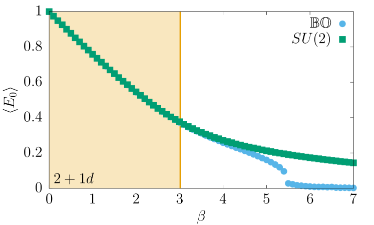
LGT calculations are performed at fixed lattice spacing which for asymptotically free theories approaches zero as . Finite leads to discrepancies from the continuum results, but provided one simulates in the scaling regime below , these errors are well-behaved. On the lattice, the breakdown of the discrete subgroup approximation manifests as a freezeout (or coupling ) where the gauge links become ”frozen” to the identity. Despite this, the approximation error for Euclidean calculations can be tolerable provided () [104, 152]. Further, a connection between the couplings and lattice spacings of Minkowski and Euclidean lattice field theories has been shown [144, 161, 153], which suggests similarly controllable digitization error on large-scale quantum simulations and a way for determining viable approximations.
The freezing transitions are known in when the Wilson action is used. Given the known connection between the Wilson action and the Kogut-Susskind Hamiltonian [162], this provides insight into the viable groups for quantum simuations. Approximating by satisfies , with . In the case of nonabelian gauge groups, there are limited number of crystal-like subgroups. , with has three: the 24-element binary tetrahedral (), the 48-element binary octahedral (), and the 120-element binary icosahedral () [104]. Thus, while require only 5 qubits, due to its low it is unlikely can be used for quantum simulation but a modified or improved Hamiltonians [80, 81] could prove sufficient [104, 128, 151, 152].
In this work, we consider the smallest crystal-like subgroup of a with – which requires 6 qubits per register. A number of smaller nonabelian groups have been considered previously. Quantum simulations of the -element dihedral groups, , while not crystal-like, have been extensively studied [101, 52, 89, 163]. The 8-element subgroup of has also been investigated [145]. In [90], quantum circuits for were constructed and resource estimates were obtained using the of [80].
In the interest of studying near-term quantum simulations, we should consider theories in addition to ones. Using classical lattice simulations, we determined in both space-times for the Wilson action (See Fig. 1). Thus quantum simulations with can be performed with the Kogut-Susskind Hamiltonian [164], although using an improved Hamiltonian can reduce either qubits or lattice spacing errors [80].
In this paper, the four necessary primitive quantum gates (inversion, multiplication, trace, and Fourier) for quantum simulation of theories on qubit-based computers are constructed. In Sec. II, important group theory for is summarized and the qubit encoding is presented. A brief review of entangling gates used is found in Sec. III. Sec. IV provides an overview of the primitive gates. This is followed by explicit quantum circuits for each gate for : the inversion gate in Sec. V, the multiplication gate in Sec. VI, the trace gate in Sec. VII, and the Fourier transform gate in Sec. VIII. Using these gates, Sec. IX presents a resource estimates for simulating . We conclude and discuss future work in Sec. X.
II Properties of
The simulation of LGT requires defining a register where one can store the state of a bosonic link variable which we call a register. Toconstruct the register in term of integers, it is necessary to map the 48 elements of to the integers . A clean way to obtain this is to write every element of as an ordered product of five generators with exponents written in terms of the binary variables with :
| (1) |
with
| (2) |
and , , are the unit quaternions which in the 2d irreducible representation (irrep) correspond to Pauli matrices. With the construction of Eq. (1), the register is given by a binary qubit encoding with the ordering . While there exist possible state in a 6 qubit register, we only consider the 48 states where represent the group elements. The states where correspond to forbidden states. In this work we will use a short hand where is the decimal representation of the binary . For example,
| (3) |
The , , and generators anti-commute with each other. Additional useful relations are:
| (4) |
| Size | 1 | 1 | 12 | 6 | 8 | 8 | 6 | 6 |
|---|---|---|---|---|---|---|---|---|
| Ord. | 1 | 2 | 4 | 4 | 6 | 3 | 8 | 8 |
| 1 | 1 | 1 | 1 | 1 | 1 | 1 | 1 | |
| 1 | 1 | 1 | 1 | 1 | ||||
| 2 | 0 | 2 | 0 | 0 | ||||
| 2 | 0 | 0 | 1 | |||||
| 2 | 0 | 0 | 1 | |||||
| 3 | 3 | 0 | 0 | 1 | 1 | |||
| 3 | 3 | 1 | 0 | 0 | ||||
| 4 | 0 | 0 | 1 | 0 | 0 | |||
| - | - | , | , | , | , | |||
| - | , | , | , | , | ||||
| , | , | , | , | , | ||||
| , | , |
The character table (Table 1) lists important group properties; the different irreps can be identified by the value of their character acting on each element. An irrep’s dimension is the value of the character of . There are three irreps, three irreps (one real and two complex), and one irrep. To derive the Fourier transform, it is necessary to know a matrix presentation of each irrep. Based on our qubit mapping, given a presentation of and we can construct any element of the group from Eq. (1). With the -th root of unity , the matrix presentations of our generators in each irrep are found in Tab. 2.
| g | -1 | ||||
|---|---|---|---|---|---|
| 1 | 1 | 1 | 1 | 1 | |
| 1 | 1 | 1 | 1 | -1 | |
III Qubit Gates
To construct our primitive gates, we chose a universal, albeit redundant, basic qubit quantum gate set. We use the Pauli gates and their arbitrary rotation generalizations . When decomposing onto fault-tolerant devices, how these are decomposed in terms of the gate becomes relevant to resource estimations.
We also use the SWAP gate
and CNOT gate
We further use the multiqubit CnNOT – of which C2NOT is called the Toffoli gate – and CSWAP (Fredkin) gates. The CnNOT gate consists of one target qubit and control qubits. For example, the Toffoli in terms of modular arithmetic is
The CSWAP gate swaps two qubit states if the control is in the state:
IV Overview of Primitive Gates
One can define any quantum circuit for gauge theories via a set of primitive gates, of which one choice is: inversion , multiplication , trace , and Fourier transform [52]. The inversion gate, , takes a -register to its inverse:
| (5) |
takes a target register and changes it to the left product controlled by a second register:
| (6) |
Left multiplication is sufficient for a minimal set as right multiplication can be obtained from two applications of and , albeit resource costs can be further reduced by an explicit construction [80].
Traces of group elements generally define the lattice Hamiltonian. We can implement the evolution with respect to these terms via:
| (7) |
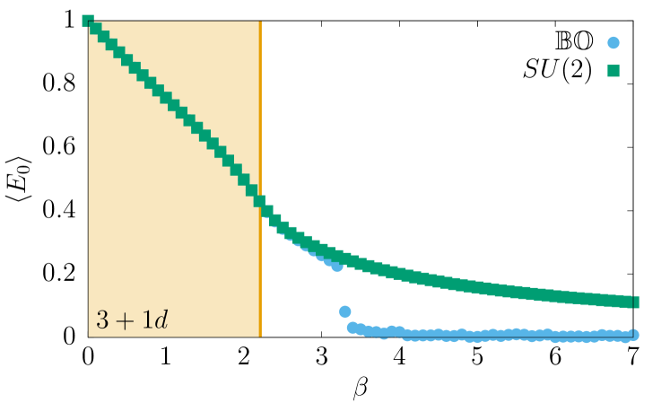
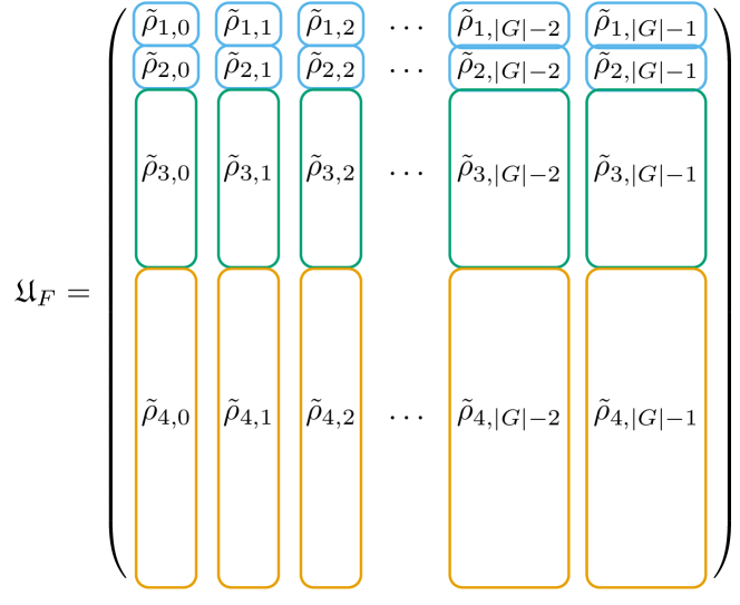
The final gate of this set is . The Fourier transform, , of a function over a finite is
| (8) |
where is the size of the group, is the dimensionality of the irreducible representation (irrep) . The inverse transform is given by
| (9) |
where the dual is the set of irreducible representations (irrep) of . A paradigm of this unitary matrix is show in Fig. 2 which can then be transformed into a gate. then acts on a single -register with some amplitudes which rotate it into the irrep basis:
| (10) |
V Inversion Gate
Consider a register storing the group element given by . The effect of the inversion gate on this register is to transform it to
| (11) |
Where must be determined. With Eq. (1), is
| (12) |
A systematic way to build the of is to embed the inverse gates of subgroups of . We start with the expression of Eq. (12), and begin by reordering the subgroup so that the element is of the form:
| (13) |
where and , . The next step is commuting thru to obtain
| (14) |
which corresponds to the inverse gate where
| (15) |
while is unchanged. Finally, commuting thru ,
| (16) |
Propagating through the portion yields where,
Finally propagating through through yields
| (17) |
with . Together, this yields for to :
| (18) |
where is unaffected.
VI Multiplication Gate
Given two registers and , we want . Here, we again decompose
| (19) |
into gates controlled by a single qubits. For each step, we use temporary variables indexed by other letters, e.g. . The first gate, , controlled by , sets:
| (20) |
Then one acts with which is controlled by :
| (21) |
where and do not change. Next, applying controlled by ,
| (22) |
with and unchanged. , controlled by , sets
| (23) |
where , and are unchanged. Then, controlled by is:
| (24) |
with thru unchanged. Finally, needs controlled by i.e. a CNOT. The full is in Fig. 4.

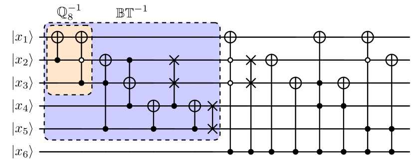
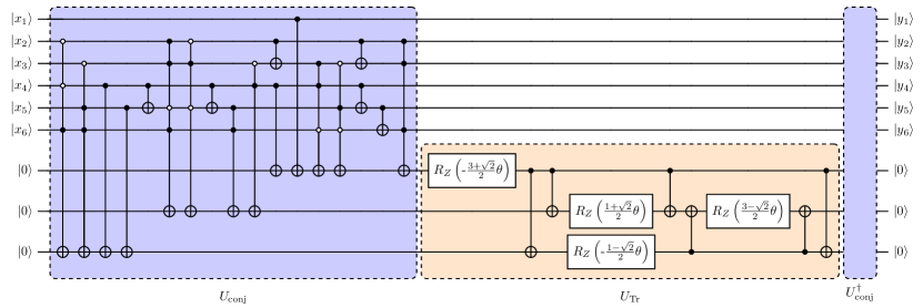
VII Trace gate
For simulating LGT, the Hamiltonian requires gauge-invariant operators. Without matter, all terms can be constructed from traces of – and thus – in the fundamental irrep, . The Tab. 1 provides us with . In previous works [52, 89, 90], was derived from a Hamiltonian, with as eigenvalues. For our -register, would require 20 Pauli strings which results in decomposing into at least 20 gates. In a fault-tolerant calculation, gates require synthesis from T gates, and thus can be unduly expensive.
Here, we explore a different implementation of that is advantageous for discrete groups where are limited by the number of conjugacy classes. In this case, could be decomposed into two gates: a gate to map the 48 to the 8 conjugacy classes , and a gate which computes the traces for each conjugacy class. Together, we obtain a circuit for which should have fewer at the cost of additional CNNOT gates which have -independent T gate costs. Taking the assignment of Table 3 for the traces we derive
where
| (25) |
A qubit-based circuit for is shown in Fig. 5. With this, we will estimate the reduction in fault-tolerant resource gate costs in Sec. IX compared to the method.
| 0 | 0 | 2 | - | 1 | - | - | ||
|---|---|---|---|---|---|---|---|---|
| 0 | 1 | 0 | 1 | 0 | 1 | 0 | 1 | |
| 0 | 0 | 1 | 1 | 0 | 0 | 1 | 1 | |
| 0 | 0 | 0 | 0 | 1 | 1 | 1 | 1 |
VIII Fourier Transform
The standard -qubit quantum Fourier transform (QFT) [166] corresponds to the quantum version of the fast Fourier transform of . Quantum Fourier transforms over some nonabelian groups exist [167, 168, 169, 170, 89]. Alas, for the crystal-like subgroups, efficient QFT circuits are currently unknown [171]. In general, no clear algorithmic way to construct the QFT exists. Thus, we instead construct a suboptimal from Eq. (8) from the irreps.
Since has 48 elements, on a qubit device must be embedded into a larger unitary. The columns index qubit bitstrings from to where the physical states are given by the subset of in Table 1. We then index the irreducible representation sequentially from to , and construct the matrix, including appropriate padding for the forbidden states. This matrix was then passed to the Qiskit v0.43.1 transpiler, and an optimized version of needed 1839 CNOTs, 166 , 1996 , and 3401 gates111In [90], the Qiskit v0.37.2 was used, yielding for the of 1025 CNOTs, 1109 , and 2139 gates. With the v0.43.1 transpiler, we obtain 442 CNOTs, 40 , 494 , and 835 .; the Fourier gate is the most expensive qubit primitive and dominates simulation costs.
IX Resource Estimates
Clearly quantum practicality with will require error corrections. Since the Eastin-Knill theorem restricts QEC codes from having a universal transversal sets of gates [172], compromises must be made. Typically, the Clifford gates are transversal [173, 174, 175, 176, 177] while the T gate is not. Thus T gate counts are often used in fault-tolerant resource analysis [173, 178]. Recently, novel universal sets have been proposed with transversal gates [179, 180, 181, 182] which deserve investigation for use with LGT.
| Gate | T gates | Clean ancilla |
|---|---|---|
| C2NOT | 7 | 0 |
| C3NOT | 21 | 1 |
| C4NOT | 35 | 2 |
| CSWAP | 7 | 0 |
| 1.15 | 0 | |
| 112 | 1 | |
| 392 | 4 | |
| 222With 6 additional ancilla, this can be reduced to | 2 | |
| 0 |
The Toffoli gate requires 7 T gates [173] and one method for constructing the CnNOT gates is with Toffoli gates and dirty ancilla qubits333A clean ancilla is in state . Dirty ancillae have unknown states. which can be reused later [183, 173, 184]. We arrive at the cost for the gates via [185] where these gates can be approximated to precision with on average T gates (and at worst [186]). Further, and can be replaced by at most 3 . With these, we can construct gate estimates for (See Tab. 4). We note that for , the 20 required for is more expensive than the constructed using .
| Gate | ||
|---|---|---|
| 2 | 4 | |
Primitive gate costs for implementing [164] and [80], per link per Trotter step are shown in Tab. 5. Using these, we can determine the total T gate count for a spatial lattice simulated for a time . We find that for
| (26) |
With this, the total synthesis error can be estimated as the sum of from each . In the case of this is
| (27) |
If one looks to reduce lattice spacing errors for a fixed number of qubits, one can use which would require
| (28) |
where the total synthesis error is
| (29) |
Following [57, 143, 90], we will make resource estimates based on our primitive gates for the calculation of the shear viscosity on a lattice evolved for , and total synthesis error of . Considering only the time evolution and neglecting state preparation (which can be substantial [20, 21, 87, 82, 187, 31, 32, 17, 33, 28, 14, 30, 84, 18, 19, 51, 12]), Kan and Nam estimated T gates would be required for an pure-gauge simulation of . This estimate used a truncated electric-field digitization which requires substantial fixed-point arithmetic – greatly inflating the T gate cost. Using , we presently estimate that T gates would be sufficient444This supersedes [90] due to the improved transpiler, proper consideration of , and better cost estimates of . but only could be used. Here, the group would require T gates if were used – albeit with smaller lattice spacing errors than Kan and Nam since they used . Thus reduces the gate costs of [143] by for fixed by avoiding quantum fixed-point arithmetic while allowing for smaller lattice spacings that . If were used the T gate cost is reduced to . Alternatively, if we take the heuristic of [80] that for using could reduce by half for fixed lattice spacing errors with only T gates. Similar to , dominates the simulations – 99% and 98% of the total cost of simulation and respectively.
X Conclusions
In this paper, we constructed the necessary primitive gates for the simulation of – a crystal-like subgroup of – gauge theories and quantum resource estimates were made for the simulation of pure shear viscosity. Compared to previous fault-tolerant qubit estimates of electric basis truncations, we require fewer T gates by avoiding quantum fixed point arithmetic via the discrete group approximation. Further, reducing digitization error compared to increase the total cost by a factor of perhaps suggesting a scaling.
Looking forward, primitive gates should be constructed for and to the subgroups of . At the cost of more qubits, would allow smaller digitization error and lattice spacings. To further reduce the qubit-based simulation gate costs for all discrete subgroup approximations, the formalism for deriving the quantum Fourier transform for crystal-like groups remains of paramount interest.
Acknowledgements.
The authors thank M. S. Alam, R. Van de Water and M. Wagman for insightful comments and support over the course of this work. EG was supported by the NASA Academic Mission Services, Contract No. NNA16BD14C. HL and FL are supported by the Department of Energy through the Fermilab QuantiSED program in the area of “Intersections of QIS and Theoretical Particle Physics”. This material is based on work supported by the U.S. Department of Energy, Office of Science, National Quantum Information Science Research Centers, Superconducting Quantum Materials and Systems Center (SQMS) under contract number DE-AC02-07CH11359 (EG). Fermilab is operated by Fermi Research Alliance, LLC under contract number DE-AC02-07CH11359 with the United States Department of Energy.References
- Klco et al. [2022] N. Klco, A. Roggero, and M. J. Savage, Standard model physics and the digital quantum revolution: thoughts about the interface, Rept. Prog. Phys. 85, 064301 (2022).
- Bañuls et al. [2020] M. C. Bañuls et al., Simulating Lattice Gauge Theories within Quantum Technologies, Eur. Phys. J. D 74, 165 (2020), arXiv:1911.00003 [quant-ph] .
- Bauer et al. [2023] C. W. Bauer et al., Quantum Simulation for High-Energy Physics, PRX Quantum 4, 027001 (2023), arXiv:2204.03381 [quant-ph] .
- Di Meglio et al. [2023] A. Di Meglio et al., Quantum Computing for High-Energy Physics: State of the Art and Challenges. Summary of the QC4HEP Working Group (2023), arXiv:2307.03236 [quant-ph] .
- Gattringer and Langfeld [2016] C. Gattringer and K. Langfeld, Approaches to the sign problem in lattice field theory, Int. J. Mod. Phys. A 31, 1643007 (2016), arXiv:1603.09517 [hep-lat] .
- Kühn et al. [2014] S. Kühn, J. I. Cirac, and M.-C. Bañuls, Quantum simulation of the Schwinger model: A study of feasibility, Phys. Rev. A 90, 042305 (2014), arXiv:1407.4995 [quant-ph] .
- Kokail et al. [2018] C. Kokail et al., Self-Verifying Variational Quantum Simulation of the Lattice Schwinger Model (2018), arXiv:1810.03421 [quant-ph] .
- Chakraborty et al. [2022] B. Chakraborty, M. Honda, T. Izubuchi, Y. Kikuchi, and A. Tomiya, Classically emulated digital quantum simulation of the Schwinger model with a topological term via adiabatic state preparation, Phys. Rev. D 105, 094503 (2022), arXiv:2001.00485 [hep-lat] .
- Yamamoto [2021a] A. Yamamoto, Quantum variational approach to lattice gauge theory at nonzero density, Phys. Rev. D 104, 014506 (2021a), arXiv:2104.10669 [hep-lat] .
- Desai et al. [2021] R. Desai, Y. Feng, M. Hassan, A. Kodumagulla, and M. McGuigan, Z3 gauge theory coupled to fermions and quantum computing (2021), arXiv:2106.00549 [quant-ph] .
- Farrell et al. [2023a] R. C. Farrell, M. Illa, A. N. Ciavarella, and M. J. Savage, Scalable Circuits for Preparing Ground States on Digital Quantum Computers: The Schwinger Model Vacuum on 100 Qubits (2023a), arXiv:2308.04481 [quant-ph] .
- Kane et al. [2023] C. F. Kane, N. Gomes, and M. Kreshchuk, Nearly-optimal state preparation for quantum simulations of lattice gauge theories (2023), arXiv:2310.13757 [quant-ph] .
- Bilgin and Boixo [2010] E. Bilgin and S. Boixo, Preparing thermal states of quantum systems by dimension reduction, Phys. Rev. Lett. 105, 170405 (2010).
- Riera et al. [2012] A. Riera, C. Gogolin, and J. Eisert, Thermalization in nature and on a quantum computer, Phys. Rev. Lett. 108, 080402 (2012).
- Lamm and Lawrence [2018] H. Lamm and S. Lawrence, Simulation of Nonequilibrium Dynamics on a Quantum Computer, Phys. Rev. Lett. 121, 170501 (2018), arXiv:1806.06649 [quant-ph] .
- Klco and Savage [2019] N. Klco and M. J. Savage, Minimally-Entangled State Preparation of Localized Wavefunctions on Quantum Computers (2019), arXiv:1904.10440 [quant-ph] .
- Harmalkar et al. [2020] S. Harmalkar, H. Lamm, and S. Lawrence (NuQS), Quantum Simulation of Field Theories Without State Preparation (2020), arXiv:2001.11490 [hep-lat] .
- Motta et al. [2020] M. Motta, C. Sun, A. T. Tan, M. J. O’Rourke, E. Ye, A. J. Minnich, F. G. Brandao, and G. K.-L. Chan, Determining eigenstates and thermal states on a quantum computer using quantum imaginary time evolution, Nature Physics 16, 205 (2020).
- de Jong et al. [2021] W. A. de Jong, K. Lee, J. Mulligan, M. Płoskoń, F. Ringer, and X. Yao, Quantum simulation of non-equilibrium dynamics and thermalization in the Schwinger model (2021), arXiv:2106.08394 [quant-ph] .
- Xie et al. [2022] X.-D. Xie, X. Guo, H. Xing, Z.-Y. Xue, D.-B. Zhang, and S.-L. Zhu (QuNu), Variational thermal quantum simulation of the lattice Schwinger model, Phys. Rev. D 106, 054509 (2022), arXiv:2205.12767 [quant-ph] .
- Davoudi et al. [2023] Z. Davoudi, N. Mueller, and C. Powers, Towards Quantum Computing Phase Diagrams of Gauge Theories with Thermal Pure Quantum States, Phys. Rev. Lett. 131, 081901 (2023), arXiv:2208.13112 [hep-lat] .
- Ball and Cohen [2023] C. Ball and T. D. Cohen, Boltzmann distributions on a quantum computer via active cooling, Nucl. Phys. A 1038, 122708 (2023), arXiv:2212.06730 [quant-ph] .
- Saroni et al. [2023] J. Saroni, H. Lamm, P. P. Orth, and T. Iadecola, Reconstructing thermal quantum quench dynamics from pure states, Phys. Rev. B 108, 134301 (2023), arXiv:2307.14508 [quant-ph] .
- Jordan et al. [2012] S. P. Jordan, K. S. M. Lee, and J. Preskill, Quantum Algorithms for Quantum Field Theories, Science 336, 1130 (2012), arXiv:1111.3633 [quant-ph] .
- Jordan et al. [2014a] S. P. Jordan, K. S. M. Lee, and J. Preskill, Quantum Computation of Scattering in Scalar Quantum Field Theories, Quant. Inf. Comput. 14, 1014 (2014a), arXiv:1112.4833 [hep-th] .
- García-Álvarez et al. [2015] L. García-Álvarez, J. Casanova, A. Mezzacapo, I. L. Egusquiza, L. Lamata, G. Romero, and E. Solano, Fermion-Fermion Scattering in Quantum Field Theory with Superconducting Circuits, Phys. Rev. Lett. 114, 070502 (2015), arXiv:1404.2868 [quant-ph] .
- Jordan et al. [2014b] S. P. Jordan, K. S. M. Lee, and J. Preskill, Quantum Algorithms for Fermionic Quantum Field Theories (2014b), arXiv:1404.7115 [hep-th] .
- Jordan et al. [2018] S. P. Jordan, H. Krovi, K. S. Lee, and J. Preskill, BQP-completeness of Scattering in Scalar Quantum Field Theory, Quantum 2, 44 (2018), arXiv:1703.00454 [quant-ph] .
- Hamed Moosavian and Jordan [2018] A. Hamed Moosavian and S. Jordan, Faster Quantum Algorithm to simulate Fermionic Quantum Field Theory, Phys. Rev. A98, 012332 (2018), arXiv:1711.04006 [quant-ph] .
- Brandão and Kastoryano [2019] F. G. Brandão and M. J. Kastoryano, Finite correlation length implies efficient preparation of quantum thermal states, Communications in Mathematical Physics 365, 1 (2019).
- Gustafson et al. [2019a] E. Gustafson, Y. Meurice, and J. Unmuth-Yockey, Quantum simulation of scattering in the quantum Ising model (2019a), arXiv:1901.05944 [hep-lat] .
- Gustafson et al. [2019b] E. Gustafson, P. Dreher, Z. Hang, and Y. Meurice, Benchmarking quantum computers for real-time evolution of a field theory with error mitigation (2019b), arXiv:1910.09478 [hep-lat] .
- Gustafson and Lamm [2021] E. J. Gustafson and H. Lamm, Toward quantum simulations of gauge theory without state preparation, Phys. Rev. D 103, 054507 (2021), arXiv:2011.11677 [hep-lat] .
- Kreshchuk et al. [2023] M. Kreshchuk, J. P. Vary, and P. J. Love, Simulating Scattering of Composite Particles (2023), arXiv:2310.13742 [quant-ph] .
- Childs et al. [2021] A. M. Childs, Y. Su, M. C. Tran, N. Wiebe, and S. Zhu, Theory of Trotter error with commutator scaling, Phys. Rev. X 11, 011020 (2021).
- Davoudi et al. [2022] Z. Davoudi, A. F. Shaw, and J. R. Stryker, General quantum algorithms for Hamiltonian simulation with applications to a non-Abelian lattice gauge theory (2022), arXiv:2212.14030 [hep-lat] .
- Campbell [2019] E. Campbell, Random compiler for fast Hamiltonian simulation, Phys. Rev. Lett. 123, 070503 (2019).
- Shaw et al. [2020] A. F. Shaw, P. Lougovski, J. R. Stryker, and N. Wiebe, Quantum Algorithms for Simulating the Lattice Schwinger Model, Quantum 4, 306 (2020), arXiv:2002.11146 [quant-ph] .
- Berry et al. [2015] D. W. Berry, A. M. Childs, R. Cleve, R. Kothari, and R. D. Somma, Simulating Hamiltonian dynamics with a truncated Taylor series, Phys. Rev. Lett. 114, 090502 (2015).
- Low and Chuang [2019] G. H. Low and I. L. Chuang, Hamiltonian Simulation by Qubitization, Quantum 3, 163 (2019).
- Berry and Childs [2012] D. W. Berry and A. M. Childs, Black-box Hamiltonian simulation and unitary implementation, Quantum Information & Computation 12 (2012).
- Low and Chuang [2017] G. H. Low and I. L. Chuang, Optimal Hamiltonian simulation by quantum signal processing, Phys. Rev. Lett. 118, 010501 (2017).
- Childs and Wiebe [2012] A. M. Childs and N. Wiebe, Hamiltonian simulation using linear combinations of unitary operations (2012).
- Cirstoiu et al. [2020] C. Cirstoiu, Z. Holmes, J. Iosue, L. Cincio, P. J. Coles, and A. Sornborger, Variational fast forwarding for quantum simulation beyond the coherence time, npj Quantum Information 6, 1 (2020).
- Gibbs et al. [2021] J. Gibbs, K. Gili, Z. Holmes, B. Commeau, A. Arrasmith, L. Cincio, P. J. Coles, and A. Sornborger, Long-time simulations with high fidelity on quantum hardware (2021), arXiv:2102.04313 [quant-ph] .
- Yao et al. [2021] Y.-X. Yao, N. Gomes, F. Zhang, C.-Z. Wang, K.-M. Ho, T. Iadecola, and P. P. Orth, Adaptive Variational Quantum Dynamics Simulations, PRX Quantum 2, 030307 (2021).
- Nagano et al. [2023] L. Nagano, A. Bapat, and C. W. Bauer, Quench dynamics of the Schwinger model via variational quantum algorithms, Phys. Rev. D 108, 034501 (2023).
- Roggero and Carlson [2018] A. Roggero and J. Carlson, Linear Response on a Quantum Computer (2018), arXiv:1804.01505 [quant-ph] .
- Roggero and Baroni [2019] A. Roggero and A. Baroni, Short-depth circuits for efficient expectation value estimation (2019), arXiv:1905.08383 [quant-ph] .
- Kanasugi et al. [2023] S. Kanasugi, S. Tsutsui, Y. O. Nakagawa, K. Maruyama, H. Oshima, and S. Sato, Computation of Green’s function by local variational quantum compilation, Phys. Rev. Res. 5, 033070 (2023), arXiv:2303.15667 [quant-ph] .
- Gustafson et al. [2023] E. J. Gustafson, H. Lamm, and J. Unmuth-Yockey, Quantum mean estimation for lattice field theory, Phys. Rev. D 107, 114511 (2023), arXiv:2303.00094 [hep-lat] .
- Lamm et al. [2019] H. Lamm, S. Lawrence, and Y. Yamauchi (NuQS), General Methods for Digital Quantum Simulation of Gauge Theories, Phys. Rev. D100, 034518 (2019), arXiv:1903.08807 [hep-lat] .
- Bauer et al. [2021a] C. W. Bauer, W. A. de Jong, B. Nachman, and D. Provasoli, Quantum Algorithm for High Energy Physics Simulations, Phys. Rev. Lett. 126, 062001 (2021a), arXiv:1904.03196 [hep-ph] .
- Echevarria et al. [2020] M. Echevarria, I. Egusquiza, E. Rico, and G. Schnell, Quantum Simulation of Light-Front Parton Correlators (2020), arXiv:2011.01275 [quant-ph] .
- Xu and Xue [2022] B. Xu and W. Xue, (3+1)-dimensional Schwinger pair production with quantum computers, Phys. Rev. D 106, 116007 (2022), arXiv:2112.06863 [quant-ph] .
- Bauer et al. [2021b] C. W. Bauer, M. Freytsis, and B. Nachman, Simulating Collider Physics on Quantum Computers Using Effective Field Theories, Phys. Rev. Lett. 127, 212001 (2021b), arXiv:2102.05044 [hep-ph] .
- Cohen et al. [2021] T. D. Cohen, H. Lamm, S. Lawrence, and Y. Yamauchi (NuQS), Quantum algorithms for transport coefficients in gauge theories, Phys. Rev. D 104, 094514 (2021), arXiv:2104.02024 [hep-lat] .
- Barata et al. [2022] J. a. Barata, X. Du, M. Li, W. Qian, and C. A. Salgado, Medium induced jet broadening in a quantum computer, Phys. Rev. D 106, 074013 (2022).
- Czajka et al. [2022] A. M. Czajka, Z.-B. Kang, Y. Tee, and F. Zhao, Studying chirality imbalance with quantum algorithms (2022), arXiv:2210.03062 [hep-ph] .
- Farrell et al. [2023b] R. C. Farrell, I. A. Chernyshev, S. J. M. Powell, N. A. Zemlevskiy, M. Illa, and M. J. Savage, Preparations for quantum simulations of quantum chromodynamics in 1+1 dimensions. II. Single-baryon -decay in real time, Phys. Rev. D 107, 054513 (2023b), arXiv:2209.10781 [quant-ph] .
- Bedaque et al. [2022] P. F. Bedaque, R. Khadka, G. Rupak, and M. Yusf, Radiative processes on a quantum computer (2022), arXiv:2209.09962 [nucl-th] .
- Ikeda et al. [2023] K. Ikeda, D. E. Kharzeev, R. Meyer, and S. Shi, Detecting the critical point through entanglement in Schwinger model (2023), arXiv:2305.00996 [hep-ph] .
- Ciavarella [2020] A. Ciavarella, Algorithm for quantum computation of particle decays, Phys. Rev. D 102, 094505 (2020), arXiv:2007.04447 [hep-th] .
- Huffman et al. [2022] E. Huffman, M. García Vera, and D. Banerjee, Toward the real-time evolution of gauge-invariant and quantum link models on noisy intermediate-scale quantum hardware with error mitigation, Phys. Rev. D 106, 094502 (2022), arXiv:2109.15065 [quant-ph] .
- Klco and Savage [2021] N. Klco and M. J. Savage, Hierarchical qubit maps and hierarchically implemented quantum error correction, Phys. Rev. A 104, 062425 (2021), arXiv:2109.01953 [quant-ph] .
- Charles et al. [2023] C. Charles, E. J. Gustafson, E. Hardt, F. Herren, N. Hogan, H. Lamm, S. Starecheski, R. S. Van de Water, and M. L. Wagman, Simulating lattice gauge theory on a quantum computer (2023), arXiv:2305.02361 [hep-lat] .
- Gustafson [2022a] E. Gustafson, Noise Improvements in Quantum Simulations of sQED using Qutrits (2022a), arXiv:2201.04546 [quant-ph] .
- Rajput et al. [2021] A. Rajput, A. Roggero, and N. Wiebe, Quantum error correction with gauge symmetries (2021), arXiv:2112.05186 [quant-ph] .
- Gustafson and Lamm [2023] E. J. Gustafson and H. Lamm, Robustness of Gauge Digitization to Quantum Noise (2023), arXiv:2301.10207 [hep-lat] .
- Halimeh and Hauke [2019] J. C. Halimeh and P. Hauke, Reliability of lattice gauge theories (2019), arXiv:2001.00024 [cond-mat.quant-gas] .
- Lamm et al. [2020] H. Lamm, S. Lawrence, and Y. Yamauchi (NuQS), Suppressing Coherent Gauge Drift in Quantum Simulations (2020), arXiv:2005.12688 [quant-ph] .
- Tran et al. [2020] M. C. Tran, Y. Su, D. Carney, and J. M. Taylor, Faster Digital Quantum Simulation by Symmetry Protection (2020), arXiv:2006.16248 [quant-ph] .
- Kasper et al. [2020] V. Kasper, T. V. Zache, F. Jendrzejewski, M. Lewenstein, and E. Zohar, Non-Abelian gauge invariance from dynamical decoupling (2020), arXiv:2012.08620 [quant-ph] .
- Halimeh et al. [2020] J. C. Halimeh, H. Lang, J. Mildenberger, Z. Jiang, and P. Hauke, Gauge-Symmetry Protection Using Single-Body Terms (2020), arXiv:2007.00668 [quant-ph] .
- Van Damme et al. [2020] M. Van Damme, J. C. Halimeh, and P. Hauke, Gauge-Symmetry Violation Quantum Phase Transition in Lattice Gauge Theories (2020), arXiv:2010.07338 [cond-mat.quant-gas] .
- Nguyen et al. [2022] N. H. Nguyen, M. C. Tran, Y. Zhu, A. M. Green, C. H. Alderete, Z. Davoudi, and N. M. Linke, Digital Quantum Simulation of the Schwinger Model and Symmetry Protection with Trapped Ions, PRX Quantum 3, 020324 (2022), arXiv:2112.14262 [quant-ph] .
- Halimeh et al. [2021] J. C. Halimeh, H. Lang, and P. Hauke, Gauge protection in non-Abelian lattice gauge theories (2021), arXiv:2106.09032 [cond-mat.quant-gas] .
- A Rahman et al. [2022] S. A Rahman, R. Lewis, E. Mendicelli, and S. Powell, Self-mitigating Trotter circuits for SU(2) lattice gauge theory on a quantum computer, Phys. Rev. D 106, 074502 (2022), arXiv:2205.09247 [hep-lat] .
- Yeter-Aydeniz et al. [2022] K. Yeter-Aydeniz, Z. Parks, A. Nair, E. Gustafson, A. F. Kemper, R. C. Pooser, Y. Meurice, and P. Dreher, Measuring NISQ Gate-Based Qubit Stability Using a 1+1 Field Theory and Cycle Benchmarking (2022), arXiv:2201.02899 [quant-ph] .
- Carena et al. [2022a] M. Carena, H. Lamm, Y.-Y. Li, and W. Liu, Improved Hamiltonians for Quantum Simulations (2022a), arXiv:2203.02823 [hep-lat] .
- Ciavarella [2023] A. N. Ciavarella, Quantum Simulation of Lattice QCD with Improved Hamiltonians (2023), arXiv:2307.05593 [hep-lat] .
- Gustafson [2022b] E. J. Gustafson, Stout Smearing on a Quantum Computer (2022b), arXiv:2211.05607 [hep-lat] .
- Temme et al. [2011] K. Temme, T. Osborne, K. Vollbrecht, D. Poulin, and F. Verstraete, Quantum Metropolis Sampling, Nature 471, 87 (2011), arXiv:0911.3635 [quant-ph] .
- Clemente et al. [2020] G. Clemente et al. (QuBiPF), Quantum computation of thermal averages in the presence of a sign problem, Phys. Rev. D 101, 074510 (2020), arXiv:2001.05328 [hep-lat] .
- Yamamoto [2022] A. Yamamoto, Quantum sampling for the Euclidean path integral of lattice gauge theory, Phys. Rev. D 105, 094501 (2022), arXiv:2201.12556 [quant-ph] .
- Ballini et al. [2023] E. Ballini, G. Clemente, M. D’Elia, L. Maio, and K. Zambello, Quantum Computation of Thermal Averages for a Non-Abelian Lattice Gauge Theory via Quantum Metropolis Sampling (2023), arXiv:2309.07090 [quant-ph] .
- Avkhadiev et al. [2020] A. Avkhadiev, P. E. Shanahan, and R. D. Young, Accelerating Lattice Quantum Field Theory Calculations via Interpolator Optimization Using Noisy Intermediate-Scale Quantum Computing, Phys. Rev. Lett. 124, 080501 (2020), arXiv:1908.04194 [hep-lat] .
- Avkhadiev et al. [2023] A. Avkhadiev, P. E. Shanahan, and R. D. Young, Strategies for quantum-optimized construction of interpolating operators in classical simulations of lattice quantum field theories, Phys. Rev. D 107, 054507 (2023), arXiv:2209.01209 [hep-lat] .
- Alam et al. [2022] M. S. Alam, S. Hadfield, H. Lamm, and A. C. Y. Li (SQMS), Primitive quantum gates for dihedral gauge theories, Phys. Rev. D 105, 114501 (2022), arXiv:2108.13305 [quant-ph] .
- Gustafson et al. [2022] E. J. Gustafson, H. Lamm, F. Lovelace, and D. Musk, Primitive quantum gates for an SU(2) discrete subgroup: Binary tetrahedral, Phys. Rev. D 106, 114501 (2022), arXiv:2208.12309 [quant-ph] .
- Zache et al. [2023a] T. V. Zache, D. González-Cuadra, and P. Zoller, Quantum and Classical Spin-Network Algorithms for q-Deformed Kogut-Susskind Gauge Theories, Phys. Rev. Lett. 131, 171902 (2023a), arXiv:2304.02527 [quant-ph] .
- Zache et al. [2023b] T. V. Zache, D. González-Cuadra, and P. Zoller, Fermion-qudit quantum processors for simulating lattice gauge theories with matter, Quantum 7, 1140 (2023b), arXiv:2303.08683 [quant-ph] .
- Zohar et al. [2012] E. Zohar, J. I. Cirac, and B. Reznik, Simulating Compact Quantum Electrodynamics with ultracold atoms: Probing confinement and nonperturbative effects, Phys. Rev. Lett. 109, 125302 (2012), arXiv:1204.6574 [quant-ph] .
- Zohar et al. [2013a] E. Zohar, J. I. Cirac, and B. Reznik, Cold-Atom Quantum Simulator for SU(2) Yang-Mills Lattice Gauge Theory, Phys. Rev. Lett. 110, 125304 (2013a), arXiv:1211.2241 [quant-ph] .
- Zohar et al. [2013b] E. Zohar, J. I. Cirac, and B. Reznik, Quantum simulations of gauge theories with ultracold atoms: local gauge invariance from angular momentum conservation, Phys. Rev. A88, 023617 (2013b), arXiv:1303.5040 [quant-ph] .
- Zohar and Burrello [2015] E. Zohar and M. Burrello, Formulation of lattice gauge theories for quantum simulations, Phys. Rev. D91, 054506 (2015), arXiv:1409.3085 [quant-ph] .
- Zohar et al. [2016] E. Zohar, J. I. Cirac, and B. Reznik, Quantum Simulations of Lattice Gauge Theories using Ultracold Atoms in Optical Lattices, Rept. Prog. Phys. 79, 014401 (2016), arXiv:1503.02312 [quant-ph] .
- Zohar et al. [2017] E. Zohar, A. Farace, B. Reznik, and J. I. Cirac, Digital lattice gauge theories, Phys. Rev. A95, 023604 (2017), arXiv:1607.08121 [quant-ph] .
- Klco et al. [2020] N. Klco, J. R. Stryker, and M. J. Savage, SU(2) non-Abelian gauge field theory in one dimension on digital quantum computers, Phys. Rev. D 101, 074512 (2020), arXiv:1908.06935 [quant-ph] .
- Ciavarella et al. [2021] A. Ciavarella, N. Klco, and M. J. Savage, A Trailhead for Quantum Simulation of SU(3) Yang-Mills Lattice Gauge Theory in the Local Multiplet Basis (2021), arXiv:2101.10227 [quant-ph] .
- Bender et al. [2018] J. Bender, E. Zohar, A. Farace, and J. I. Cirac, Digital quantum simulation of lattice gauge theories in three spatial dimensions, New J. Phys. 20, 093001 (2018), arXiv:1804.02082 [quant-ph] .
- Liu and Xin [2020] J. Liu and Y. Xin, Quantum simulation of quantum field theories as quantum chemistry (2020), arXiv:2004.13234 [hep-th] .
- Hackett et al. [2019] D. C. Hackett, K. Howe, C. Hughes, W. Jay, E. T. Neil, and J. N. Simone, Digitizing Gauge Fields: Lattice Monte Carlo Results for Future Quantum Computers, Phys. Rev. A 99, 062341 (2019), arXiv:1811.03629 [quant-ph] .
- Alexandru et al. [2019] A. Alexandru, P. F. Bedaque, S. Harmalkar, H. Lamm, S. Lawrence, and N. C. Warrington (NuQS), Gluon field digitization for quantum computers, Phys.Rev.D 100, 114501 (2019), arXiv:1906.11213 [hep-lat] .
- Yamamoto [2021b] A. Yamamoto, Real-time simulation of (2+1)-dimensional lattice gauge theory on qubits, PTEP 2021, 013B06 (2021b), arXiv:2008.11395 [hep-lat] .
- Haase et al. [2021] J. F. Haase, L. Dellantonio, A. Celi, D. Paulson, A. Kan, K. Jansen, and C. A. Muschik, A resource efficient approach for quantum and classical simulations of gauge theories in particle physics, Quantum 5, 393 (2021), arXiv:2006.14160 [quant-ph] .
- Armon et al. [2021] T. Armon, S. Ashkenazi, G. García-Moreno, A. González-Tudela, and E. Zohar, Photon-mediated Stroboscopic Quantum Simulation of a Lattice Gauge Theory (2021), arXiv:2107.13024 [quant-ph] .
- Bazavov et al. [2019] A. Bazavov, S. Catterall, R. G. Jha, and J. Unmuth-Yockey, Tensor renormalization group study of the non-abelian higgs model in two dimensions, Phys. Rev. D 99, 114507 (2019).
- Bazavov et al. [2015] A. Bazavov, Y. Meurice, S.-W. Tsai, J. Unmuth-Yockey, and J. Zhang, Gauge-invariant implementation of the Abelian Higgs model on optical lattices, Phys. Rev. D92, 076003 (2015), arXiv:1503.08354 [hep-lat] .
- Zhang et al. [2018] J. Zhang, J. Unmuth-Yockey, J. Zeiher, A. Bazavov, S. W. Tsai, and Y. Meurice, Quantum simulation of the universal features of the Polyakov loop, Phys. Rev. Lett. 121, 223201 (2018), arXiv:1803.11166 [hep-lat] .
- Unmuth-Yockey et al. [2018] J. Unmuth-Yockey, J. Zhang, A. Bazavov, Y. Meurice, and S.-W. Tsai, Universal features of the Abelian Polyakov loop in 1+1 dimensions, Phys. Rev. D98, 094511 (2018), arXiv:1807.09186 [hep-lat] .
- Unmuth-Yockey [2019] J. F. Unmuth-Yockey, Gauge-invariant rotor Hamiltonian from dual variables of 3D gauge theory, Phys. Rev. D 99, 074502 (2019), arXiv:1811.05884 [hep-lat] .
- Kreshchuk et al. [2020a] M. Kreshchuk, W. M. Kirby, G. Goldstein, H. Beauchemin, and P. J. Love, Quantum Simulation of Quantum Field Theory in the Light-Front Formulation (2020a), arXiv:2002.04016 [quant-ph] .
- Kreshchuk et al. [2020b] M. Kreshchuk, S. Jia, W. M. Kirby, G. Goldstein, J. P. Vary, and P. J. Love, Simulating Hadronic Physics on NISQ devices using Basis Light-Front Quantization (2020b), arXiv:2011.13443 [quant-ph] .
- Raychowdhury and Stryker [2018] I. Raychowdhury and J. R. Stryker, Solving Gauss’s Law on Digital Quantum Computers with Loop-String-Hadron Digitization (2018), arXiv:1812.07554 [hep-lat] .
- Raychowdhury and Stryker [2020] I. Raychowdhury and J. R. Stryker, Loop, String, and Hadron Dynamics in SU(2) Hamiltonian Lattice Gauge Theories, Phys. Rev. D 101, 114502 (2020), arXiv:1912.06133 [hep-lat] .
- Davoudi et al. [2020] Z. Davoudi, I. Raychowdhury, and A. Shaw, Search for Efficient Formulations for Hamiltonian Simulation of non-Abelian Lattice Gauge Theories (2020), arXiv:2009.11802 [hep-lat] .
- Wiese [2014] U.-J. Wiese, Towards Quantum Simulating QCD, Proceedings, 24th International Conference on Ultra-Relativistic Nucleus-Nucleus Collisions (Quark Matter 2014): Darmstadt, Germany, May 19-24, 2014, Nucl. Phys. A931, 246 (2014), arXiv:1409.7414 [hep-th] .
- Luo et al. [2019] D. Luo, J. Shen, M. Highman, B. K. Clark, B. DeMarco, A. X. El-Khadra, and B. Gadway, A Framework for Simulating Gauge Theories with Dipolar Spin Systems (2019), arXiv:1912.11488 [quant-ph] .
- Brower et al. [2019] R. C. Brower, D. Berenstein, and H. Kawai, Lattice Gauge Theory for a Quantum Computer, PoS LATTICE2019, 112 (2019), arXiv:2002.10028 [hep-lat] .
- Mathis et al. [2020] S. V. Mathis, G. Mazzola, and I. Tavernelli, Toward scalable simulations of Lattice Gauge Theories on quantum computers, Phys. Rev. D 102, 094501 (2020), arXiv:2005.10271 [quant-ph] .
- Singh [2019] H. Singh, Qubit nonlinear sigma models (2019), arXiv:1911.12353 [hep-lat] .
- Singh and Chandrasekharan [2019] H. Singh and S. Chandrasekharan, Qubit regularization of the sigma model, Phys. Rev. D 100, 054505 (2019), arXiv:1905.13204 [hep-lat] .
- Buser et al. [2020] A. J. Buser, T. Bhattacharya, L. Cincio, and R. Gupta, State preparation and measurement in a quantum simulation of the (3) sigma model, Phys. Rev. D 102, 114514 (2020), arXiv:2006.15746 [quant-ph] .
- Bhattacharya et al. [2021] T. Bhattacharya, A. J. Buser, S. Chandrasekharan, R. Gupta, and H. Singh, Qubit regularization of asymptotic freedom, Phys. Rev. Lett. 126, 172001 (2021), arXiv:2012.02153 [hep-lat] .
- Barata et al. [2020] J. a. Barata, N. Mueller, A. Tarasov, and R. Venugopalan, Single-particle digitization strategy for quantum computation of a scalar field theory (2020), arXiv:2012.00020 [hep-th] .
- Kreshchuk et al. [2020c] M. Kreshchuk, S. Jia, W. M. Kirby, G. Goldstein, J. P. Vary, and P. J. Love, Light-Front Field Theory on Current Quantum Computers (2020c), arXiv:2009.07885 [quant-ph] .
- Ji et al. [2020] Y. Ji, H. Lamm, and S. Zhu (NuQS), Gluon Field Digitization via Group Space Decimation for Quantum Computers, Phys. Rev. D 102, 114513 (2020), arXiv:2005.14221 [hep-lat] .
- Bauer and Grabowska [2021] C. W. Bauer and D. M. Grabowska, Efficient Representation for Simulating U(1) Gauge Theories on Digital Quantum Computers at All Values of the Coupling (2021), arXiv:2111.08015 [hep-ph] .
- Gustafson [2021] E. Gustafson, Prospects for Simulating a Qudit Based Model of (1+1)d Scalar QED, Phys. Rev. D 103, 114505 (2021), arXiv:2104.10136 [quant-ph] .
- Hartung et al. [2022] T. Hartung, T. Jakobs, K. Jansen, J. Ostmeyer, and C. Urbach, Digitising SU(2) gauge fields and the freezing transition, Eur. Phys. J. C 82, 237 (2022), arXiv:2201.09625 [hep-lat] .
- Grabowska et al. [2022] D. M. Grabowska, C. Kane, B. Nachman, and C. W. Bauer, Overcoming exponential scaling with system size in Trotter-Suzuki implementations of constrained Hamiltonians: 2+1 U(1) lattice gauge theories (2022), arXiv:2208.03333 [quant-ph] .
- Murairi et al. [2022] E. M. Murairi, M. J. Cervia, H. Kumar, P. F. Bedaque, and A. Alexandru, How many quantum gates do gauge theories require? (2022), arXiv:2208.11789 [hep-lat] .
- Hasenfratz and Niedermayer [2001a] P. Hasenfratz and F. Niedermayer, Asymptotic freedom with discrete spin variables?, Proceedings, 2001 Europhysics Conference on High Energy Physics (EPS-HEP 2001): Budapest, Hungary, July 12-18, 2001, PoS HEP2001, 229 (2001a), arXiv:hep-lat/0112003 [hep-lat] .
- Caracciolo et al. [2001a] S. Caracciolo, A. Montanari, and A. Pelissetto, Asymptotically free models and discrete nonAbelian groups, Phys. Lett. B513, 223 (2001a), arXiv:hep-lat/0103017 [hep-lat] .
- Hasenfratz and Niedermayer [2001b] P. Hasenfratz and F. Niedermayer, Asymptotically free theories based on discrete subgroups, Lattice field theory. Proceedings, 18th International Symposium, Lattice 2000, Bangalore, India, August 17-22, 2000, Nucl. Phys. Proc. Suppl. 94, 575 (2001b), arXiv:hep-lat/0011056 [hep-lat] .
- Patrascioiu and Seiler [1998] A. Patrascioiu and E. Seiler, Continuum limit of two-dimensional spin models with continuous symmetry and conformal quantum field theory, Phys. Rev. E 57, 111 (1998).
- Krcmar et al. [2016] R. Krcmar, A. Gendiar, and T. Nishino, Phase diagram of a truncated tetrahedral model, Phys. Rev. E 94, 022134 (2016).
- Caracciolo et al. [2001b] S. Caracciolo, A. Montanari, and A. Pelissetto, Asymptotically free models and discrete non-abelian groups, Physics Letters B 513, 223 (2001b).
- Zhou et al. [2022] J. Zhou, H. Singh, T. Bhattacharya, S. Chandrasekharan, and R. Gupta, Spacetime symmetric qubit regularization of the asymptotically free two-dimensional O(4) model, Phys. Rev. D 105, 054510 (2022), arXiv:2111.13780 [hep-lat] .
- Caspar and Singh [2022] S. Caspar and H. Singh, From asymptotic freedom to vacua: Qubit embeddings of the O(3) nonlinear model (2022), arXiv:2203.15766 [hep-lat] .
- Zohar [2021] E. Zohar, Quantum Simulation of Lattice Gauge Theories in more than One Space Dimension – Requirements, Challenges, Methods (2021), arXiv:2106.04609 [quant-ph] .
- Kan and Nam [2021] A. Kan and Y. Nam, Lattice Quantum Chromodynamics and Electrodynamics on a Universal Quantum Computer (2021), arXiv:2107.12769 [quant-ph] .
- Carena et al. [2021] M. Carena, H. Lamm, Y.-Y. Li, and W. Liu, Lattice renormalization of quantum simulations, Phys. Rev. D 104, 094519 (2021), arXiv:2107.01166 [hep-lat] .
- González-Cuadra et al. [2022] D. González-Cuadra, T. V. Zache, J. Carrasco, B. Kraus, and P. Zoller, Hardware efficient quantum simulation of non-abelian gauge theories with qudits on Rydberg platforms (2022), arXiv:2203.15541 [quant-ph] .
- Creutz et al. [1979] M. Creutz, L. Jacobs, and C. Rebbi, Monte Carlo Study of Abelian Lattice Gauge Theories, Phys. Rev. D20, 1915 (1979).
- Creutz and Okawa [1983] M. Creutz and M. Okawa, Generalized Actions in ) Lattice Gauge Theory, Nucl. Phys. B220, 149 (1983).
- Bhanot and Rebbi [1981] G. Bhanot and C. Rebbi, Monte Carlo Simulations of Lattice Models With Finite Subgroups of SU(3) as Gauge Groups, Phys. Rev. D24, 3319 (1981).
- Petcher and Weingarten [1980] D. Petcher and D. H. Weingarten, Monte Carlo Calculations and a Model of the Phase Structure for Gauge Theories on Discrete Subgroups of SU(2), Phys. Rev. D22, 2465 (1980).
- Bhanot [1982] G. Bhanot, SU(3) Lattice Gauge Theory in Four-dimensions With a Modified Wilson Action, Phys. Lett. 108B, 337 (1982).
- Ji et al. [2022] Y. Ji, H. Lamm, and S. Zhu, Gluon Digitization via Character Expansion for Quantum Computers (2022), arXiv:2203.02330 [hep-lat] .
- Alexandru et al. [2022] A. Alexandru, P. F. Bedaque, R. Brett, and H. Lamm, Spectrum of digitized QCD: Glueballs in a S(1080) gauge theory, Phys. Rev. D 105, 114508 (2022), arXiv:2112.08482 [hep-lat] .
- Carena et al. [2022b] M. Carena, E. J. Gustafson, H. Lamm, Y.-Y. Li, and W. Liu, Gauge theory couplings on anisotropic lattices, Phys. Rev. D 106, 114504 (2022b), arXiv:2208.10417 [hep-lat] .
- Weingarten and Petcher [1981] D. H. Weingarten and D. N. Petcher, Monte Carlo Integration for Lattice Gauge Theories with Fermions, Phys. Lett. 99B, 333 (1981).
- Weingarten [1982] D. Weingarten, Monte Carlo Evaluation of Hadron Masses in Lattice Gauge Theories with Fermions, Phys. Lett. 109B, 57 (1982), [,631(1981)].
- Kogut [1980] J. B. Kogut, 1/n Expansions and the Phase Diagram of Discrete Lattice Gauge Theories With Matter Fields, Phys. Rev. D 21, 2316 (1980).
- Romers [2007] J. Romers, Discrete gauge theories in two spatial dimensions, Ph.D. thesis, Master’s thesis, Universiteit van Amsterdam (2007).
- Fradkin and Shenker [1979] E. H. Fradkin and S. H. Shenker, Phase Diagrams of Lattice Gauge Theories with Higgs Fields, Phys. Rev. D 19, 3682 (1979).
- Harlow and Ooguri [2018] D. Harlow and H. Ooguri, Symmetries in quantum field theory and quantum gravity (2018), arXiv:1810.05338 [hep-th] .
- Horn et al. [1979] D. Horn, M. Weinstein, and S. Yankielowicz, Hamiltonian Approach to Z(N) Lattice Gauge Theories, Phys. Rev. D 19, 3715 (1979).
- Clemente et al. [2022] G. Clemente, A. Crippa, and K. Jansen, Strategies for the determination of the running coupling of (2+1)-dimensional QED with quantum computing, Phys. Rev. D 106, 114511 (2022), arXiv:2206.12454 [hep-lat] .
- Creutz [1985] M. Creutz, Quarks, gluons and lattices, Cambridge Monographs on Mathematical Physics (Cambridge Univ. Press, Cambridge, UK, 1985).
- Fromm et al. [2022] M. Fromm, O. Philipsen, and C. Winterowd, Dihedral Lattice Gauge Theories on a Quantum Annealer (2022), arXiv:2206.14679 [hep-lat] .
- Kogut and Susskind [1975] J. Kogut and L. Susskind, Hamiltonian formulation of Wilson’s lattice gauge theories, Phys. Rev. D 11, 395 (1975).
- Grimus and Ludl [2012] W. Grimus and P. O. Ludl, Finite flavour groups of fermions, J. Phys. A 45, 233001 (2012), arXiv:1110.6376 [hep-ph] .
- Nielsen and Chuang [2010] M. A. Nielsen and I. L. Chuang, Quantum Computation and Quantum Information: 10th Anniversary Edition (Cambridge University Press, 2010).
- Hoyer [1997] P. Hoyer, Efficient quantum transforms (1997), arXiv:quant-ph/9702028 [quant-ph] .
- Beals [1997] R. Beals, Quantum computation of Fourier transforms over symmetric groups, in Proceedings of the twenty-ninth annual ACM symposium on Theory of computing (Citeseer, 1997) pp. 48–53.
- Püschel et al. [1999] M. Püschel, M. Rötteler, and T. Beth, Fast quantum Fourier transforms for a class of non-abelian groups, in International Symposium on Applied Algebra, Algebraic Algorithms, and Error-Correcting Codes (Springer, 1999) pp. 148–159.
- Moore et al. [2006] C. Moore, D. Rockmore, and A. Russell, Generic quantum Fourier transforms, ACM Transactions on Algorithms (TALG) 2, 707 (2006).
- Childs and van Dam [2010] A. M. Childs and W. van Dam, Quantum algorithms for algebraic problems, Rev. Mod. Phys. 82, 1 (2010).
- Eastin and Knill [2009] B. Eastin and E. Knill, Restrictions on transversal encoded quantum gate sets, Phys. Rev. Lett. 102, 110502 (2009).
- Chuang and Nielsen [1997] I. L. Chuang and M. A. Nielsen, Prescription for experimental determination of the dynamics of a quantum black box, J. Mod. Opt. 44, 2455 (1997), arXiv:quant-ph/9610001 .
- Calderbank and Shor [1996] A. R. Calderbank and P. W. Shor, Good quantum error-correcting codes exist, Phys. Rev. A 54, 1098 (1996), arXiv:quant-ph/9512032 [quant-ph] .
- Steane [1996] A. M. Steane, Error correcting codes in quantum theory, Phys. Rev. Lett. 77, 793 (1996).
- Steane [1996] A. Steane, Multiple-Particle Interference and Quantum Error Correction, Proceedings of the Royal Society of London Series A 452, 2551 (1996), arXiv:quant-ph/9601029 [quant-ph] .
- Steane [1996] A. M. Steane, Simple quantum error-correcting codes, Phys. Rev. A 54, 4741 (1996).
- Kitaev [1997] A. Y. Kitaev, Quantum computations: algorithms and error correction, Russian Mathematical Surveys 52, 1191 (1997).
- Kubischta and Teixeira [2023] E. Kubischta and I. Teixeira, A Family of Quantum Codes with Exotic Transversal Gates (2023), arXiv:2305.07023 [quant-ph] .
- Denys and Leverrier [2023a] A. Denys and A. Leverrier, Multimode bosonic cat codes with an easily implementable universal gate set (2023a), arXiv:2306.11621 [quant-ph] .
- Jain et al. [2023] S. P. Jain, J. T. Iosue, A. Barg, and V. V. Albert, Quantum spherical codes (2023), arXiv:2302.11593 [quant-ph] .
- Denys and Leverrier [2023b] A. Denys and A. Leverrier, The -qutrit, a two-mode bosonic qutrit, Quantum 7, 1032 (2023b), arXiv:2210.16188 [quant-ph] .
- Baker et al. [2019] J. M. Baker, C. Duckering, A. Hoover, and F. T. Chong, Decomposing Quantum Generalized Toffoli with an Arbitrary Number of Ancilla (2019), arXiv:1904.01671 [quant-ph] .
- Barenco et al. [1995] A. Barenco, C. H. Bennett, R. Cleve, D. P. DiVincenzo, N. Margolus, P. Shor, T. Sleator, J. A. Smolin, and H. Weinfurter, Elementary gates for quantum computation, Phys. Rev. A 52, 3457 (1995).
- Bocharov et al. [2015] A. Bocharov, M. Roetteler, and K. M. Svore, Efficient synthesis of universal repeat-until-success quantum circuits, Phys. Rev. Lett. 114, 080502 (2015).
- Selinger [2015] P. Selinger, Efficient clifford+t approximation of single-qubit operators, Quantum Info. Comput. 15, 159–180 (2015).
- Peruzzo et al. [2014] A. Peruzzo, J. McClean, P. Shadbolt, M.-H. Yung, X.-Q. Zhou, P. J. Love, A. Aspuru-Guzik, and J. L. O’brien, A variational eigenvalue solver on a photonic quantum processor, Nature communications 5, 4213 (2014).