Building symmetries into data-driven manifold dynamics models for complex flows

Abstract

Symmetries in a dynamical system provide an opportunity to dramatically improve the performance of data-driven models. For fluid flows, such models are needed for tasks related to design, understanding, prediction, and control. In this work we exploit the symmetries of the Navier-Stokes equations (NSE) and use simulation data to find the manifold where the long-time dynamics live, which has many fewer degrees of freedom than the full state representation, and the evolution equation for the dynamics on that manifold. We call this method “symmetry charting”. The first step is to map to a “fundamental chart”, which is a region in the state space of the flow to which all other regions can be mapped by a symmetry operation. To map to the fundamental chart we identify a set of indicators from the Fourier transform that uniquely identify the symmetries of the system. We then find a low-dimensional coordinate representation of the data in the fundamental chart with the use of an autoencoder. We use a variation called an implicit rank minimizing autoencoder with weight decay, which in addition to compressing the dimension of the data, also gives estimates of how many dimensions are needed to represent the data: i.e. the dimension of the invariant manifold of the long-time dynamics. Finally, we learn dynamics on this manifold with the use of neural ordinary differential equations. We apply symmetry charting to two-dimensional Kolmogorov flow in a chaotic bursting regime. This system has a continuous translation symmetry, and discrete rotation and shift-reflect symmetries. With this framework we observe that less data is needed to learn accurate data-driven models, more robust estimates of the manifold dimension are obtained, equivariance of the NSE is satisfied, better short-time tracking with respect to the true data is observed, and long-time statistics are correctly captured.

I Introduction

In recent years, neural networks (NNs) have been implemented to learn data-driven low-dimensional representations and dynamical models of flow problems, with success in systems including the Moehlis-Faisst-Eckhardt (MFE) model [1], Kolmogorov flow [2, 3], and minimal turbulent channel flow [4]. For the most part however, these approaches do not explicitly take advantage of the fact that for dissipative systems like the Navier-Stokes Equations (NSE), the long-time dynamics are expected to lie on an invariant manifold $\mathcal{M}$ (sometimes called an inertial manifold [5, 6, 7]), $d_{\mathcal{M}}$, whose dimension may be much smaller than the nominal number of degrees of freedom $N$ required to specify the state of the system. Ideally, one could identify $d_{\mathcal{M}}$ from data, find a coordinate representation for points on $\mathcal{M}$, and learn the time-evolution on $\mathcal{M}$ in those coordinates. This would be a minimal-dimensional data-driven dynamic model. Linot & Graham explored this approach for chaotic dynamics of the Kuramoto-Sivashinsky equation (KSE) [8, 9]. They showed that the mean-squared error (MSE) of the reconstruction of the snapshots using an autoencoder (AE) for dimension reduction for the domain size of $L=22$ exhibited an orders-of-magnitude drop when the dimension of the inertial manifold is reached. Furthermore, modeling the dynamics with a dense NN at this dimension either with a discrete-time map [8] or a system of ordinary differential equations (ODE) [9] yielded excellent trajectory predictions and long-time statistics. The approach they introduced is referred to here as data-driven manifold dynamics (DManD). For the KSE in larger domains, it was found that simply observing MSE vs. autoencoder bottleneck dimension was not sufficient to determine the manifold dimension and exhaustive tests involving time evolution models vs. dimension were necessary to estimate the manifold dimension. Pérez De Jesús & Graham extended this approach to two-dimensional Kolmogorov flow in a chaotic regime [10]. Here dimension reduction from 1024 dimensions to $\leq 10$ was achieved, with very good short-time tracking predictions, long-time statistics, as well as accurate predictions of bursting events. Linot & Graham considered three-dimensional direct numerical simulations of turbulent Couette flow at $\text{Re}=400$ and found accurate data-driven dynamic models with fewer than 20 degrees of freedom [11]. These models were able to capture characteristics of the flows such as streak breakdown and regeneration, short-time tracking, as well as Reynolds stresses and energy balance. They also computed unstable periodic orbits from the models with close resemblance to previously computed orbits from the full system. Relatedly, Zeng et al. [12] exploited advances in autoencoder architecture [13] to yield more precise estimates of $d_{\mathcal{M}}$ for data from high-dimensional chaotic systems. The present work illustrates how symmetries of a flow system can be exploited in the DManD framework to yield highly efficient low-dimensional data-driven models for chaotic flows.

A fundamental notion in the topology of manifolds, which will be useful in exploiting symmetry, is that of charts and atlases [14]. Simply put, a chart is a region of a manifold whose points can be represented in a local Cartesian coordinate system of dimension $d_{\mathcal{M}}$ and which overlaps with neighboring charts, while an atlas is a collection of charts that covers the manifold. This representation of a manifold has several advantages. First, for a manifold with dimension $d_{\mathcal{M}}$, it may not be possible to find a global coordinate representation in $d_{\mathcal{M}}$ dimensions: Whitney’s embedding theorem states that generic smooth maps for a smooth manifold of dimension $d_{\mathcal{M}}$ can be embedded into a Euclidean space of $2d_{\mathcal{M}}$. Dividing a manifold into an atlas of charts enables minimal-dimensional representations locally in $d_{\mathcal{M}}$ dimensions. Second, from the dynamical point of view, dynamics on different parts of a manifold may be very different and a single global representation of a manifold and the dynamics on it may not efficiently capture the dynamics, especially in the data-driven context. These two advantages of an atlas-of-charts representation have been exploited for data-driven modeling. Floryan & Graham developed a method to implement data-driven local representations for dynamical systems such as the quasiperiodic dynamics on a torus, a reaction-diffusion system, and the KSE to learn dynamics on invariant manifolds of minimal dimension [15]. They refer to this method as Charts and Atlases for Nonlinear Data-Driven Dynamics on Manifolds – “CANDyMan”. Fox et al. then applied this to the MFE model, which displays highly intermittent behavior in the form of quasilaminarization and full relaminarization events, demonstrating more accurate time evolution predictions as global (“single chart”) model [16]. In the present work, we use the charts and atlases framework to exploit symmetries.

In the Navier-Stokes equations (NSE), symmetries appear in the form of continuous and discrete symmetry groups. The symmetries of the NSE in physical space are reflected in state space as symmetries of the vector field, and these can generate natural charts of the system. Consider the vector field $\boldsymbol{q}$ shown in Fig. 1a where the operation $\mathcal{R}\boldsymbol{q}$ rotates the vector field by $\pi/2$ in the clockwise direction. Trajectories of the ODE $\dot{\boldsymbol{y}}=\boldsymbol{q}$ will reflect this symmetry. Without exploiting symmetry, any model trained on this data will need to represent the whole state space and even so will generally not obey the exact symmetries of the true system due to finite sampling effects. In this work we leverage knowledge of the charts by explicitly considering and factoring out the symmetries. We show a depiction of this in Fig. 1b where we know that by applying $\mathcal{R}$ to the data we can map it to a different quadrant, and that by mapping points in quadrants 2, 3, and 4 with $\mathcal{R}$, $\mathcal{R}^{2}$, and $\mathcal{R}^{3}$, respectively, they all end up in quadrant 1. This is shown in Fig. 1c where the data collapses on top of each other when mapped to the first quadrant. We will call this region the “fundamental domain” for the state space, and when expanded to overlap with its neighbors, the “fundamental chart”.

Some previous work has focused on factoring out symmetries of dynamical systems for dimension reduction in the data-driven context. However, symmetries have not been considered explicitly for data-driven reduced-order models (ROMs). Kneer et al. built symmetries into an AE architecture for dimension reduction and applied it to the Kolmogorov flow system [17]. With the use of branches that receive the different discrete symmetries of the snapshots and spatial transformer networks that manipulate the continuous phase, they were able to map to a fundamental domain by selecting the branch that gives the smallest MSE and backpropagating through it. By doing this, the AE naturally selects a path that leads to the lowest MSE of reconstruction while considering the symmetries of the system. The purpose of this work was not to find the minimal dimension or learn ROMs. Budanur & Cvitanovic formulated a symmetry-reducing scheme, previously applied to the Lorenz equations [18], to the KSE, where a polynomial transformation of the Fourier modes combined with the method-of-slices for factoring out spatial phase leads to a mapping in the fundamental domain [19]. Applying this method to more complicated systems, such as Kolmogorov flow, may be quite challenging. Symmetry reduction has also been successfully used for controlling the KSE with synthetic jets. Zeng & Graham applied discrete symmetry operations to map the state to the fundamental domain, and used this as the input to a reinforcement learning control agent, the performance of which is dramatically improved by exploitation of symmetry[20].

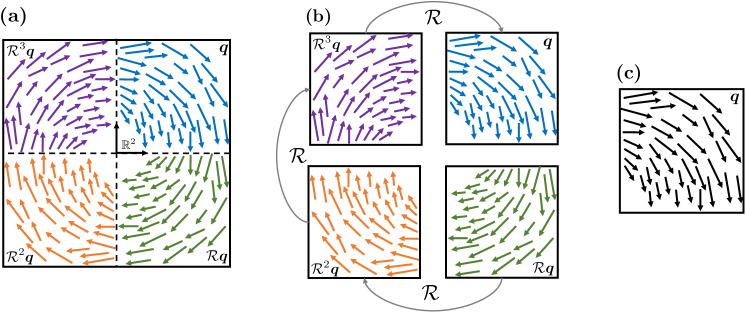
Figure 1: (a) Vector field $\boldsymbol{q}$ with symmetry group $\mathcal{R}$ in state space. (b) Data in each quadrant can be mapped to another quadrant by operating with $\mathcal{R}$. (c) After mapping everything to the positive quadrant data lies on top of each other.

In the present work, we present a framework for learning DManD models in the fundamental chart, as in Fig. 1c, where the dynamics of the flow occur, and apply it to chaotic dynamics of the NSE. We refer to this method as “symmetry charting”, which results in (at least approximately) minimal-dimensional data-driven models that are equivariant to symmetry operations. In addition the model only need to be learned in one chart because a combination of its symmetric versions will cover the manifold. We first learn minimal-dimensional representations in the fundamental chart followed by an evolution equation for the dynamics on it. To this end we use information about the symmetries of the system combined with NNs to learn the compressed representation and dynamics.

We apply symmetry charting to two-dimensional Kolmogorov flow in a regime where the chaotic dynamics travels between unstable relative periodic orbits (RPOs) [21] through bursting events [22] that shadow heteroclinic orbits connecting the RPOs. RPOs correspond to periodic orbits in a moving reference frame, such that in a fixed frame, the pattern at time $t+T$ is a phase-shifted replica of the pattern at time $t$. To achieve this goal we map the data to a fundamental chart which is then used to train undercomplete AEs to find low-dimensional representations. To this end, we use Implicit Rank Minimizing autoencoders with weight decay (IRMAE-WD) [12]. This architecture was introduced by Zeng & Graham as a method that estimates $d_{\mathcal{M}}$ without the need to sweep over dimensions and using MSE and statistics as indicators [8, 10]. We give an overview of IRMAE-WD in Section III.2. After learning a low-dimensional representation with IRMAE-WD we learn a time map with the use of the neural ODE (NODE) [23], which we discuss in Section III.3. We then show results in Section IV and finish with concluding remarks in Section V.

II Kolmogorov flow, symmetries, and projections

The two-dimensional NSE with Kolmogorov forcing are

$$\frac{\partial\boldsymbol{u}}{\partial t}+\boldsymbol{u}\cdot\boldsymbol{\nabla}\boldsymbol{u}+\boldsymbol{\nabla}p=\frac{1}{\mathrm{Re}}\nabla^{2}\boldsymbol{u}+\sin(ny)\hat{\boldsymbol{x}},$$ (1)

$$\nabla\cdot\boldsymbol{u}=0,$$ (2)

where flow is in the $x-y$ plane, $\boldsymbol{u}=[u,v]$ is the velocity vector, $p$ is the pressure, $n$ is the wavenumber of the forcing, and $\hat{\boldsymbol{x}}$ is the unit vector in the $x$ direction. Here $\mathrm{Re}=\frac{\sqrt{\chi}}{v}\left(\frac{L_{y}}{2\pi}\right)^{3/2}$ where $\chi$ is the dimensional forcing amplitude, $\nu$ is the kinematic viscosity, and $L_{y}$ is the size of the domain in the $y$ direction. We consider the periodic domain $[0,2\pi/\alpha]\times[0,2\pi]$ with $\alpha=1$. Vorticity is defined as $\omega=\hat{\boldsymbol{z}}\cdot\boldsymbol{\nabla}\times\boldsymbol{u}$, where $\hat{\boldsymbol{z}}$ is the unit vector in the $z$ direction (orthogonal to the flow). The equations are invariant under several symmetry operations [24], namely a shift (in $y$)-reflect (in $x$), a rotation through $\pi$, and a continuous translation in $x$:

$$\mathscr{S}:[u,v,\omega](x,y)\rightarrow[-u,v,-\omega]\left(-x,y+\frac{\pi}{n}\right),$$ (3)

$$\mathscr{R}:[u,v,\omega](x,y)\rightarrow[-u,-v,\omega](-x,-y),$$ (4)

$$\mathscr{T}_{l}:[u,v,\omega](x,y)\rightarrow[u,v,\omega](x+l,y).$$ (5)

For $n$ wavelengths the state can be shift-reflected $2n-1$ times with the operation $\mathscr{S}$. Together with the rotation $\mathscr{R}$ there will be a total of $4n$ states that are related by symmetries. In the case of $n=2$ this results in eight regions of state space that are related to one another by symmetries. In the chaotic regime that we consider, trajectories visit each of these regions. Relatedly, velocity fields for the Kolmogorov flow satisfy the equivarance property associated with these actions: if $\boldsymbol{u}$ is a solution at a given time, then so are $\mathscr{S}\boldsymbol{u}$, $\mathscr{R}\boldsymbol{u}$, and $\mathscr{T}_{l}\boldsymbol{u}$. We elaborate on this property in Sec. III.1.

The total kinetic energy for this system ($KE$), dissipation rate ($D$) and power input ($I$) are

$$KE=\frac{1}{2}\left\langle\boldsymbol{u}^{2}\right\rangle_{V},D=\frac{1}{\mathrm{Re}}\left\langle|\nabla\boldsymbol{u}|^{2}\right\rangle_{V},\quad I=\langle u\sin(ny)\rangle_{V}$$ (6)

where $\left\langle\cdot\right\rangle_{V}$ corresponds to the average taken over the domain. For the case of $n=1$ the laminar state is linearly stable at all Re [25]. It is not until $n=2$ that the laminar state becomes unstable, with a critical value of $\mathrm{Re}_{c}=n^{3/2}2^{1/4}$[26, 27, 28]. In what follows, we evolve the NSE numerically in the vorticity representation on a $[d_{x}\times d_{y}]=[32\times 32]$ grid following the pseudo-spectral scheme given by Chandler & Kerswell [24], which is based on the code by Bartello & Warn [29].

In Fig. 2 we show the time-series evolution of $\|\omega(t)\|$, where $\|\cdot\|$ is the $l^{2}$-norm, for an RPO obtained at $\text{Re}=13.5$, $n=2$, as well as the state-space projection of the trajectory into the subspace $\hat{\omega}_{R}(0,1)-\hat{\omega}_{I}(0,1)-\hat{\omega}_{I}(0,2)$ where $\hat{\omega}(k_{x},k_{y},t)=\mathcal{F}\{\omega(x,y,t)\}=\hat{\omega}_{R}(k_{x},k_{y},t)+i\hat{\omega}_{I}(k_{x},k_{y},t)$ is the discrete Fourier transform in $x$ and $y$, and subscripts $R$ and $I$ correspond to real and imaginary parts. We also consider chaotic Kolmogorov flow with $\text{Re}=14.4$, $n=2$. Fig. 3 shows the time-series evolution of $\|\omega(t)\|$ as well as the state-space projection of the trajectory into the subspace $\hat{\omega}_{R}(0,1)-\hat{\omega}_{I}(0,1)-\hat{\omega}_{I}(0,2)$ for this chaotic regime. Due to the discrete symmetries of the system, there are several RPOs [22]. The dynamics are characterized by quiescent intervals where the trajectories approach the RPOs (which are now unstable), punctuated by fast excursions between the RPOs, which are indicated by the intermittent increases of the $\|\omega(t)\|$ in Fig. 3(a). Under the projection shown in Fig. 3(b), we see four RPOs, which initially seems surprising as there are eight discrete symmetries and a continuous symmetry. However, the continuous symmetry is removed under this projection (it will only appear for $k_{x}\neq 0$), and the discrete symmetry operations of $\mathscr{R}$ and $\mathscr{S}$ will flip the signs of $\hat{\omega}_{R}(0,1)$, $\hat{\omega}_{I}(0,1)$, and $\hat{\omega}_{I}(0,2)$ such that portions of the different RPOs are covered. Specifics of the sign changes will be made clear in Section III.1.

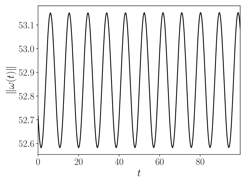
(a)

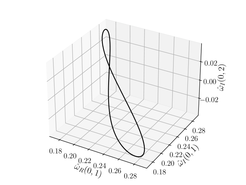
(b)

Figure 2: (a) Time evolution of $\|\omega(t)\|$ at $\mathrm{Re}=13.5$. (b) State-space projection of the trajectory into the subspace $\hat{\omega}_{R}(0,1)-\hat{\omega}_{I}(0,1)-\hat{\omega}_{I}(0,2)$ for $\mathrm{Re}=13.5$.

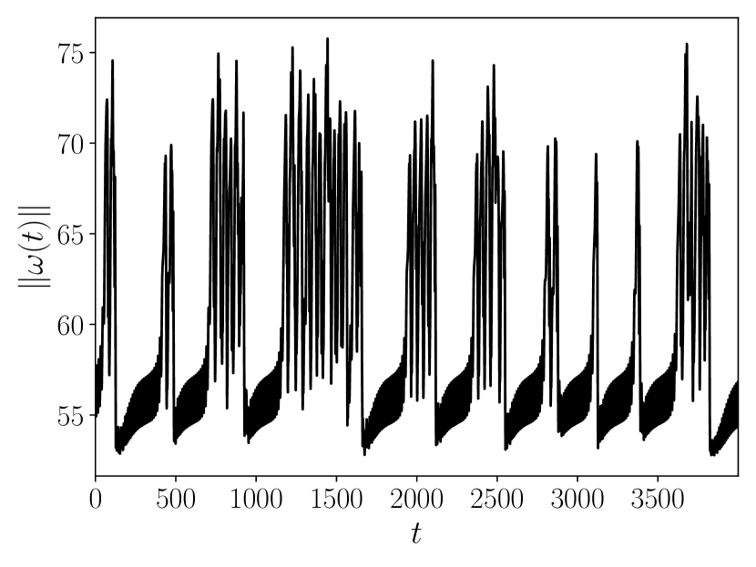
(a)

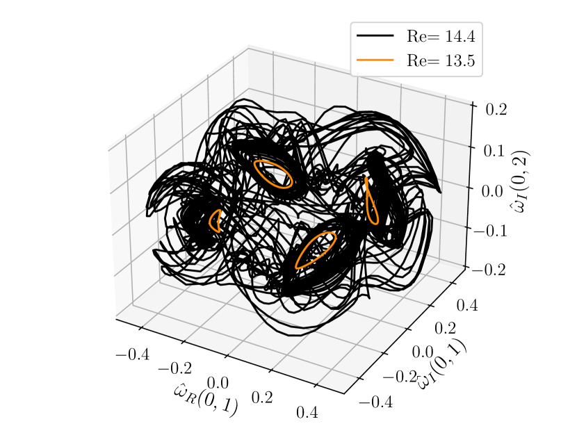
(b)

Figure 3: (a) Time evolution of $\|\omega(t)\|$ at $\mathrm{Re}=14.4$. (b) State-space projection of the trajectory into the subspace $\hat{\omega}_{R}(0,1)-\hat{\omega}_{I}(0,1)-\hat{\omega}_{I}(0,2)$ for $\mathrm{Re}=13.5$ and $\mathrm{Re}=14.4$.

III Data-driven dimension reduction and dynamic modeling

In the following sections, we describe the steps involved in symmetry charting: 1) mapping data to the fundamental space, 2) finding a minimal-dimensional coordinate representation, and 3) evolving the minimal-dimensional state and symmetry indicators forward through time. The parts of this procedure separating it from other data-driven reduced order models are how we map to the fundamental and how we evolve the symmetry indicators through time. Our approach guarantees equivariance under symmetry operations.

III.1 Map to fundamental domain

First we discuss a method to map trajectories of Kolmogorov flow to the fundamental domain where symmetries are factored out [30]. The first step is to identify a set of indicators that are related to the group of symmetries. In order to find these indicators we consider the effect of these symmetry operations in Fourier space. After Fourier transforming the equations and simplifying these are the actions of the symmetry operations on the Fourier coefficients:

$$\mathscr{S}:\hat{\omega}(k_{x},k_{y})\rightarrow-\hat{\omega}(-k_{x},k_{y})e^{ik_{y}\pi/n},$$ (7)

$$\mathscr{R}:\hat{\omega}(k_{x},k_{y})\rightarrow\bar{\hat{\omega}}(k_{x},k_{y}),$$ (8)

$$\mathscr{T}_{l}:\hat{\omega}(k_{x},k_{y})\rightarrow\hat{\omega}(k_{x},k_{y})e^{-ik_{x}l},$$ (9)

where $\bar{\cdot}$ denotes the complex conjugate.

Now, we will show how these symmetry operations act on the Fourier coefficients in specific ways that we can exploit to classify any given state as lying within a specific region or domain of state space. We refer to this classification of the continuous symmetry as the “phase” and the discrete symmetry as the “indicator”. To compute the phase and remove the continuous symmetry $\mathscr{T}_{l}$, we use the First Fourier mode method-of-slices [31, 32]. This method involves computing the spatial phase $\phi_{x}$ of the $k_{x}=1$ and $k_{y}=0$ Fourier mode: $\phi_{x}(t)=\operatorname{atan}2\left\{\hat{\omega}_{I}(1,0),\hat{\omega}_{R}(1,0)\right\}$. Then, to phase-align the data, we shift the vorticity snapshots such that this mode is a pure cosine: $\omega_{l}(x,y,t)=\mathcal{F}^{-1}\left\{\mathcal{F}\{\omega(x,y,t)\}e^{-ik\phi_{x}(t)}\right\}$. Doing this ensures that the snapshots lie in a reference frame where no translation happens in the $x$ direction. From Eq. 9 we see that this operation only modifies Fourier coefficients with $k_{x}\neq 0$. Thus, if we use $k_{x}=0$ coefficients to determine the discrete indicator it will be independent of the phase.

For the shift-reflect operation, we consider the $(k_{x}=0,k_{y}=1)$ mode. In Eq. 7 the shift-reflect operation modifies this Fourier coefficient in this manner: $\hat{\omega}_{R}(0,1)+i\hat{\omega}_{I}(0,1)\rightarrow\hat{\omega}_{I}(0,1)-i\hat{\omega}_{R}(0,1)$. This shows that the shift-reflect operation maps between different quadrants of the $\hat{\omega}_{R}(0,1)-\hat{\omega}_{I}(0,1)$ plane. Next, we consider the rotation operation on the $(k_{x}=0,k_{y}=2)$ mode. In Eq. 8 we see this operation simply flips the sign of the imaginary component $\hat{\omega}_{I}(0,2)\rightarrow-\hat{\omega}_{I}(0,2)$. Thus, applying the eight possible discrete symmetry operations (including the identity operation) to a vorticity field will map us to eight unique points in the $\hat{\omega}_{R}(0,1)$, $\hat{\omega}_{I}(0,1)$, $\hat{\omega}_{I}(0,2)$ space. As such, we may classify each octant with an $\mathcal{I}$ between $0-7$. This means that any snapshot can be mapped to a fundamental domain and be uniquely identified by $\mathcal{I}$. In Fig. 4 we show the indicators for $\text{Re}=13.5$. The colored curves correspond to the sections of the different RPOs that are related by discrete symmetries. Notice that each section of the different RPOs can be uniquely identified by $\mathcal{I}$. Table 1 shows how any snapshot in any octant can be mapped to the $\mathcal{I}=0$ octant by applying the corresponding discrete symmetry operations. These same indicators extend to the chaotic case $\text{Re}=14.4$ and in the rest of this work we refer to the fundamental domain as the space corresponding to $\mathcal{I}=0$. Fig. 5 shows the state-space projection of a chaotic trajectory at $\text{Re}=14.4$ into the region $\hat{\omega}_{R}(0,1)-\hat{\omega}_{I}(0,1)-\hat{\omega}_{I}(0,2)$, where the different colors give the indicator for the chart in which that data point lies. More generally, we note that any point in the state space of the system can represented by a point in the fundamental domain along with an indicator $\mathcal{I}$ and phase $\phi_{x}$.

This representation is satisfactory for static data, but not for modeling trajectories represented in the fundamental domain, because when a trajectory exits one region, its corresponding trajectory in the fundamental domain leaves there and instantaneously enters at a different point: i.e. the time evolution is discontinuous in this representation.

To address this issue we use the concept of charts and atlases that is fundamental to the study of manifolds [14], in a way that is closely related to that of Floryan & Graham [15]. An atlas for a manifold is a collection of patches, each of which must overlap with its neighbors, that are called charts. In each chart, a local coordinate representation can be found, and for each pair of overlapping charts, a transition map takes coordinates in one chart to those in the neighboring one – with this coordinate tranformation there are no discontinuities. To use this formalism in the present case requires us to expand the fundamental domain so that it overlaps with its neighbors, so the fundamental chart is simply the fundamental domain, comprised of “interior points” plus the overlap region (“exterior points”), and there are seven other charts, each generated by the symmetry operation acting on the fundamental chart including the overlap regions. We choose a coordinate representation for all charts that corresponds to that for the fundamental chart, and for a trajectory that leaves the fundamental domain with e.g. $\mathcal{I}=4$ and reenters with $\mathcal{I}=6$, the transition map is the function that moves the point in the fundamental chart from the “exit” of the $\mathcal{I}=4$ chart to the “entrance” of the $\mathcal{I}=6$ chart.

In Fig. 5(a) we show the state space projection of a trajectory, identifying interior points with solid markers and exterior points with open markers. We isolate the region close to an RPO in Fig. 5(b) to make this more clear. Solid markers correspond to data points that lie in the interior of a chart. Open markers correpond to the data points in the connecting chart that will be included together with the interior data. Many different approaches can be taken to identify points to include in the exterior. Here we simply identified all points in a small volume around each octant as exterior points. We did this by finding the dimensions of a box surrounding the octant (by calculating the maximum absolute value in the $\hat{\omega}_{R}(0,1)-\hat{\omega}_{I}(0,1)-\hat{\omega}_{I}(0,2)$ directions) and then increasing the size of this box by expanding each direction $20\%$. Any point that lies in the volume between the octant and this expanded domain is an exterior point. We varied the percent increase to $5\%$, $10\%$, and $30\%$ and observed no change in the results.

Now that we have identified these exterior points we can continue with the procedure of mapping the data to the fundamental chart. To do this, we apply the appropriate discrete operations to the interior and exterior points of each chart to map the state such that the interior points fall in $\mathcal{I}=0$ ($\hat{\omega}_{R}(0,1)>0$, $\hat{\omega}_{I}(0,1)>0$, $\hat{\omega}_{I}(0,2)>0$). Fig. 6(a) shows the colored clusters mapped onto the positive octant, dark blue cluster. Figures 6(b) and 6(c) show projections in the planes $\hat{\omega}_{R}(0,1)-\hat{\omega}_{I}(0,1)$ and $\hat{\omega}_{R}(0,1)-\hat{\omega}_{I}(0,2)$ respectively of data mapped to the positive octant. The dashed lines correspond to the boundaries between the different octants. We see clearly that mapping the data to the fundamental chart leads to a much higher density of data points and thus to better sampling than if we considered the whole state space without accounting for the symmetries. Following the mapping to the fundamental chart we phase-align the snapshots and refer to this data as $\tilde{\omega}$ from this point on.

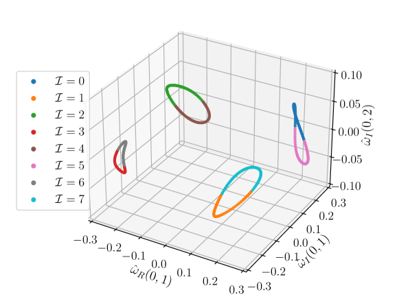
Figure 4: State-space projection of the different RPOs into the plane $\hat{\omega}_{R}(0,1)-\hat{\omega}_{I}(0,1)-\hat{\omega}_{I}(0,2)$ for $\mathrm{Re}=13.5$. The different colors are for different discrete symmetry indicators which are shown in the legend.

Table 1: Indicators $\mathcal{I}$ and the corresponding operations required to map to $\mathcal{I}=0$

$$\begin{array}[]{cc}\hline\cr\hline\cr\mathcal{I}&\text{\; \; \; \; Discrete operations }\\ \hline\cr 0&\text{None}\\ 1&\mathscr{R}\omega\\ 2&\mathscr{S}^{3}\omega\\ 3&\mathscr{S}^{3}\mathscr{R}\omega\\ 4&\mathscr{S}^{2}\mathscr{R}\omega\\ 5&\mathscr{S}\mathscr{R}\omega\\ 6&\mathscr{S}^{2}\omega\\ 7&\mathscr{S}\omega\\ \hline\cr\hline\cr\end{array}$$

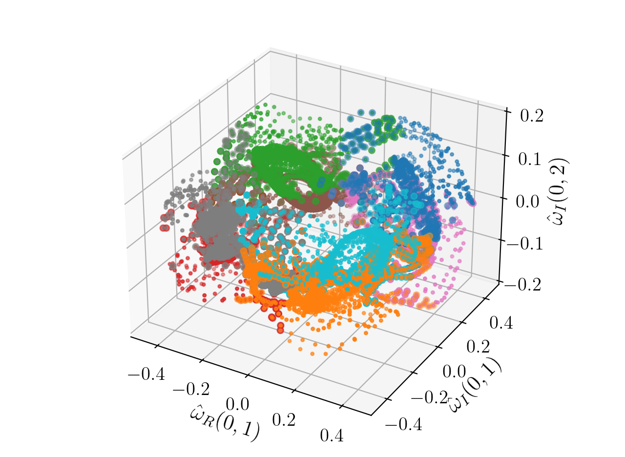
(a)

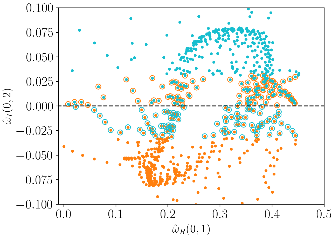
(b)

Figure 5: (a) State-space projection of a trajectory into the subspace $\hat{\omega}_{R}(0,1)-\hat{\omega}_{I}(0,1)-\hat{\omega}_{I}(0,2)$ for $\mathrm{Re}=14.4$. Colors correspond to the discrete symmetry indicator. (b) Zoom into the region near the RPO corresponding to $\mathcal{I}=1,7$. Solid markers correspond to interior points and open markers to exterior points – e.g.  the blue solid markers within an open orange marker are in the interior region of chart 7 and exterior region of chart 1.

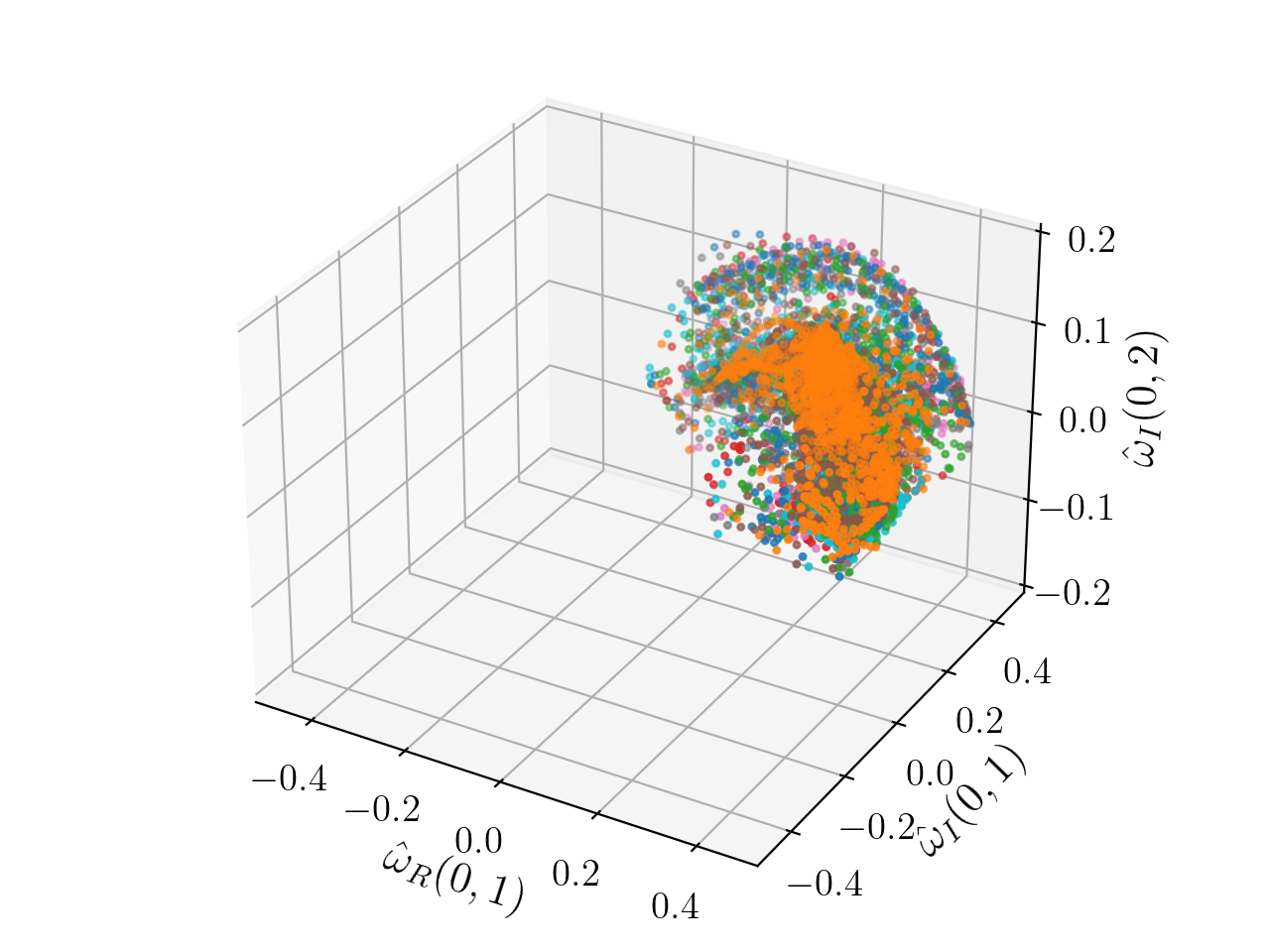
(a)

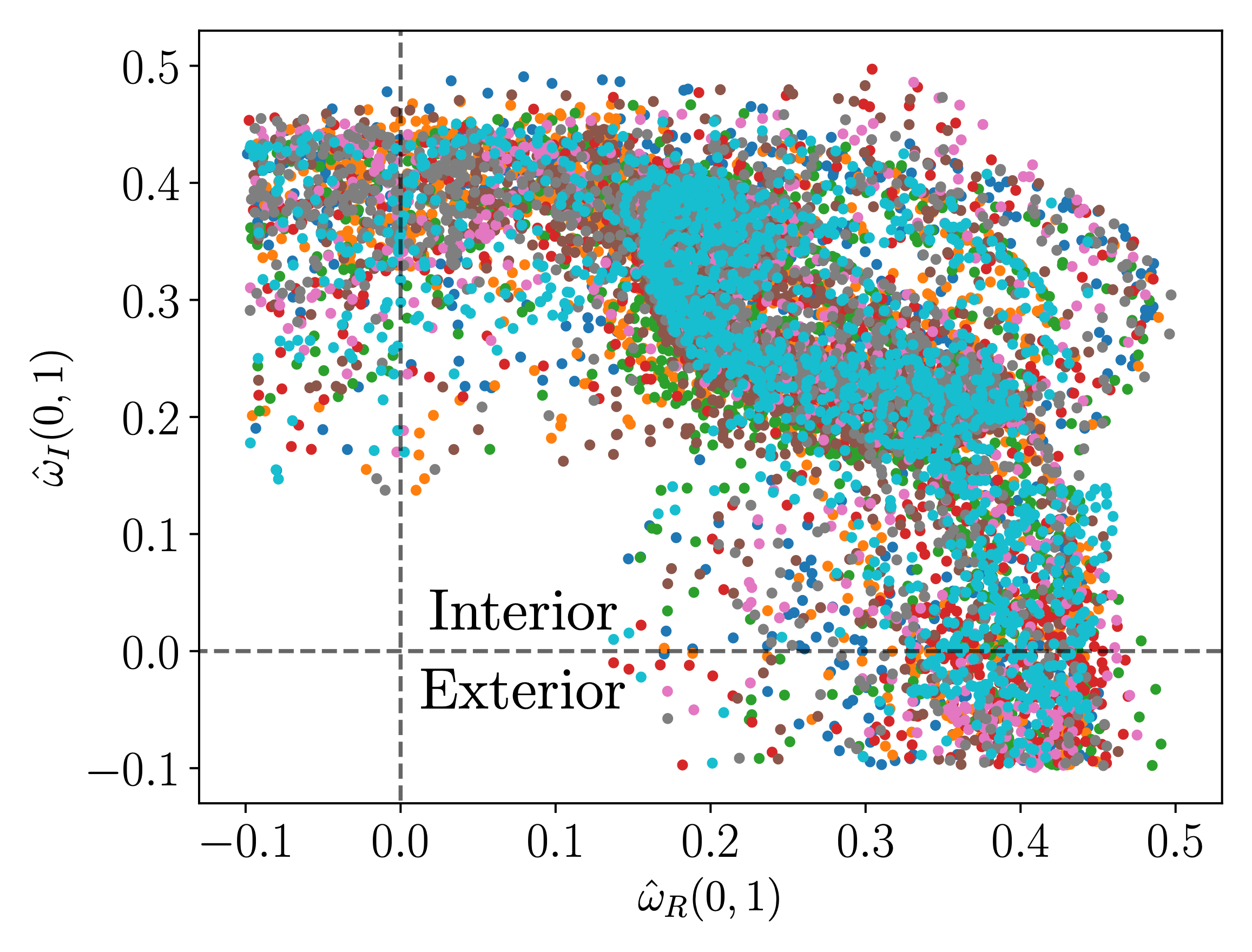
(b)

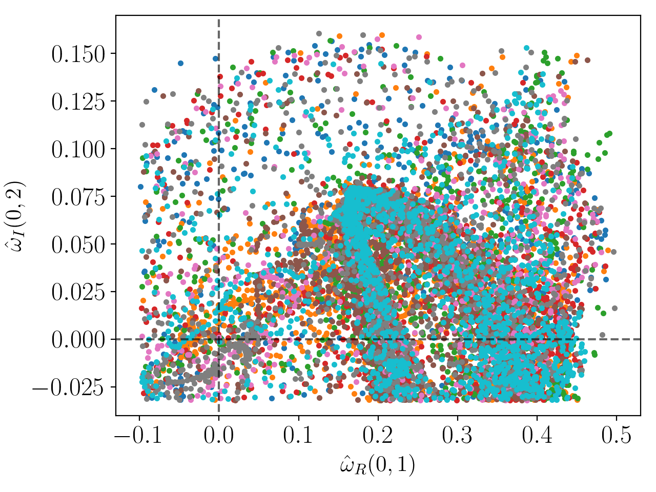
(c)

Figure 6: (a) Snapshots mapped to the fundamental chart ($\hat{\omega}_{R}(0,1)>0$, $\hat{\omega}_{I}(0,1)>0$, $\hat{\omega}_{I}(0,2)>0$). (b) and (c) are the state-space projection of the trajectory into the planes $\hat{\omega}_{R}(0,1)-\hat{\omega}_{I}(0,1)$ and $\hat{\omega}_{R}(0,1)-\hat{\omega}_{I}(0,2)$, respectively. The dotted lines give the boundary between interior and exterior points.

III.2 Finding a manifold coordinate representation with IRMAE-WD

In the previous section we discussed how to obtain the fundamental chart. We have defined a natural subdivision of the state space, where the invariant manifold of the dynamics is represented by an atlas of charts that are related by symmetry operations. This means that we do not need to learn the full invariant manifold, only the piece in the fundamental chart. To find a low-dimensional representation of the fundamental chart we use a variant of a common machine-learning architecture known as an undercomplete autoencoder (AE), whose purpose is to learn a reduced representation of the state such that the reconstruction error with respect to the true data is minimized. We flatten the vorticity field $\tilde{\omega}$ such that $N=32\times 32=1024$. The AE consists of an encoder and a decoder. The encoder maps from the full space $\tilde{\omega}\in\mathbb{R}^{N}$ to the lower-dimensional latent space $h(t)\in\mathbb{R}^{d_{h}}$, where ideally $d_{h}=d_{\mathcal{M}}\ll N$, and the decoder maps back to the full space $\tilde{\omega}_{r}$.

Previous works have focused on tracking MSE and dynamic model performance as $d_{h}$ varies to find good low-dimensional representations [8, 11, 10]. This is a tedious trial-and-error process that in general does not yield a precise estimate of $d_{\mathcal{M}}$. Other works have learned compressed representations of flow problems [2, 3, 4]. However, performance over a systematic range of $d_{h}$ is not examined in these cases. A more systematic alternative would be highly desirable. In recent work, Zeng et al. [12] showed that a straightforward variation on a standard autoencoder can yield robust and precise estimates of $d_{\mathcal{M}}$ for a range of systems, as well as an orthogonal manifold coordinate system. The architecture they study is called an Implicit Rank Minimizing Autoencoder with weigh decay (IRMAE-WD), and involves inserting a series of linear layers between the encoder and decoder and adding an $L_{2}$ regularization on the neural network weights in the loss. The effect of these additions is an AE for which the standard gradient descent algorithm for learning NN weights drives the rank of the covariance of the data in the latent representation to a minimum while maintaining representational capability. Applying this to the KSE and other systems resulted in the rank being equal to the dimension of the inertial manifold $d_{\mathcal{M}}$. IRMAE was originally presented by Jing et al. [13] to learn low-rank representations for image-based classification and generative problems.

Fig. 7a shows the IRMAE-WD framework. The encoder, denoted by $E\left(\tilde{\omega};\theta_{E}\right)$ reduces the dimension from $N$ to $d_{z}$. We then include a linear network $\mathcal{W}\left(\cdot;\theta_{W}\right)$ between the encoder and the decoder which consists of several linear layers (matrix multiplications). Finally, the decoder $\tilde{\omega}_{r}=D\left(z;\theta_{D}\right)$ maps back to the full space. An $L_{2}$ (“weight decay”) regularization to the weights is also added, with prefactor $\lambda$. The loss function for this architecture is

$$\mathcal{L}\left(\tilde{\omega};\theta_{E},\theta_{W},\theta_{D}\right)=\left\langle\left\|\tilde{\omega}-D\left(\mathcal{W}\left(E\left(\tilde{\omega};\theta_{E}\right);\theta_{W}\right);\theta_{D}\right)\right\|_{2}^{2}\right\rangle+\frac{\lambda}{2}\|\theta\|_{2}^{2}.$$ (10)

where $\langle\cdot\rangle$ is the average over a training batch, $\theta_{E}$ the weights of the encoder, $\theta_{D}$ the weights of the decoder, and $\theta_{W}$ the weights of the linear network. Zeng et al. [12] found dimension estimates for the KSE to be robust to the number of linear layers, $\lambda$, and $d_{z}$. However, as we will show, there is more variability when selecting these parameters for Kolmogorov flow. Nevertheless, we will see that IRMAE-WD yields a robust estimate of the upper bound of $d_{\mathcal{M}}$ that proves very useful.

After training, we can perform SVD on the covariance matrix of the encoded data matrix $Z$ to obtain the singular vectors $U$ and singular values $S$ as shown in Fig. 7b. Projecting $z$ onto $\hat{U}^{T}$ gives an orthogonal representation $h^{+}=U^{T}z$ as illustrated in Fig. 7c. Then, by choosing only the singular values above some very small threshold (typically $\gtrsim 6$ orders of magnitude smaller than the leading singular values), we may project down to fewer dimensions by projecting onto the corresponding singular vectors $U$, denoted $\hat{U}$ to yield the low-rank manifold representation $h=\hat{U}z$ (Fig. 7d). We refer to Table 2 for details on the architecture.

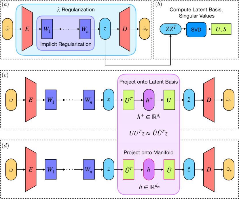
Figure 7: Implicit Rank Minimizing autoencoder with weight decay (IRMAE-WD) framework: a) network architecture with regularization mechanisms, b) singular value decomposition of the covariance of the learned latent data representation $Z$, c) projection of latent variables onto manifold coordinates d) isolated projection of latent variables onto manifold coordinates. Image reproduced with permission from [12].

III.3 Time evolution of pattern with neural ODEs

In the previous two steps we first mapped our data to the fundamental chart, allowing us to represent the state with $\tilde{\omega}$, $\mathcal{I}$, and $\phi_{x}$. Then we reduced the dimension of $\tilde{\omega}$ by mapping it to the manifold coordinates $h$. Next, we need to find a method to evolve $h$, $\mathcal{I}$, and $\phi$ through time. To forecast $h(t)$ in time we use the neural ODE (NODE) framework[9, 33, 23]. We use a stabilized version proposed by Linot et. al. [33] where the dynamics on the manifold in the fundamental chart are described by the equation

$$\frac{dh}{dt}=g_{h}(h)-Ah.$$ (11)

Here $A$ is chosen to have a stabilizing effect that keeps solutions from blowing up. We can define this parameter as $A=\text{diag}(\kappa[\text{std}(h)$]) where $\kappa=0.1$ is multiplied by the element-wise standard deviation of $h$. The value of $\kappa$ can be changed, but we see good prediction for the selected value. The equation is integrated to estimate $h_{r}(t+\tau)$ as

$$h_{r}\left(t+\tau\right)=h\left(t\right)+\int_{t}^{t+\tau}(g_{h}\left(h(t^{\prime});\theta_{t}\right)-Ah)dt^{\prime}$$ (12)

where $\theta_{t}$ are the weights of the NN $g_{h}$, refer to Table 2, which are determined by minimizing the loss

$$\mathcal{L}_{\text{NODE}}\left(h;\theta_{t}\right)=\left\langle\left\|h(t+\tau)-h_{r}(t+\tau)\right\|_{2}^{2}\right\rangle.$$ (13)

To train the NODE model we first gather $\omega(t)$ and $\omega(t+\tau)$. We then map to the fundamental chart in pairs. As an example, if a snapshot $\omega(t)$ lies in $\mathcal{I}=5$ we apply the corresponding discrete operations such that $h(t)$ falls in the interior of the fundamental chart $\mathcal{I}=0$. The same discrete operations, which are $\mathscr{S}\mathscr{R}$ (refer to Table 1), are applied to $\omega(t+\tau)$. This means that $h(t+\tau)$ does not need to fall in the interior. We select $\tau=0.5$ which is a small enough time such that the exterior region is covered by the autoencoder.

Now that we trained the NODE models we want to evolve trajectories in time. To do this we need to track the pattern $h$ and the indicator $\mathcal{I}$ at every time. We first show an exit and entry in the state space representation in Fig. 8. The initial condition (IC) starts in $\mathcal{I}=0$ and exits through the bottom part of the domain. Looking at Fig. 4 we see that this corresponds to a transition from $\mathcal{I}=0$ to $\mathcal{I}=5$. Hence, to keep evolving in the fundamental chart we need to apply the corresponding discrete operations to map to $\mathcal{I}=0$ and keep track of the new indicator $\mathcal{I}=5$. Notice that we need to keep track of the new indicator to map back to the full space at the end. This can generalize to a longer trajectory in which case the indicator changes depending on where the trajectory leaves the fundamental chart. The transitions between indicators corresponding to the different charts are shown in Fig. 9. Here we see a graph representation of the connections between the 8 symmetry charts for a trajectory of $10^{5}$ snapshots. The intensity of each connection is related to the probability of the trajectory transitioning to another chart. The four darker lines correspond to the shadowing of the RPOs and the lighter lines are related to the bursting events. Now that we know how the indicators change we can evolve initial conditions with the NODE models to obtain predicted trajectories in $h$.

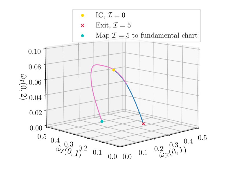
(a)

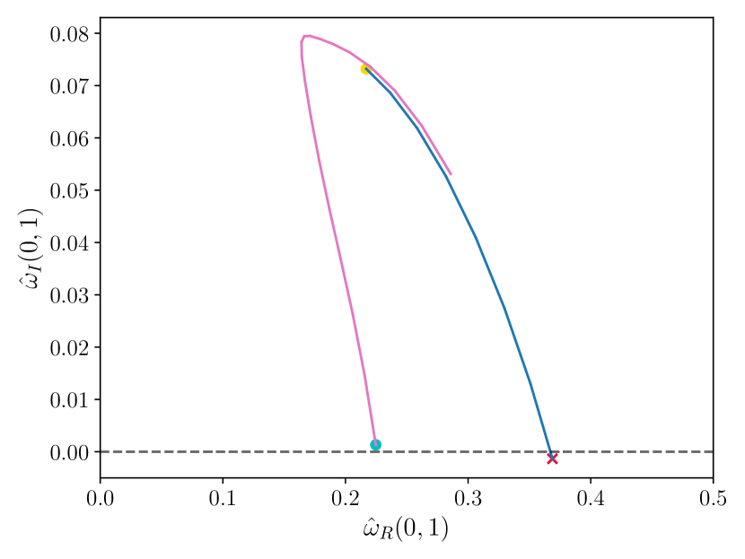
(b)

Figure 8: (a) Initial condition (IC) starting at $\mathcal{I}=0$ is evolved and exits into the chart $\mathcal{I}=5$. This exit is mapped back to $\mathcal{I}=0$ to keep evolving in the fundamental chart. (b) Two-dimensional projection showing the exit from the fundamental chart. Here we selected an IC near the RPO, which is the reason why this trajectory nearly closes on itself.

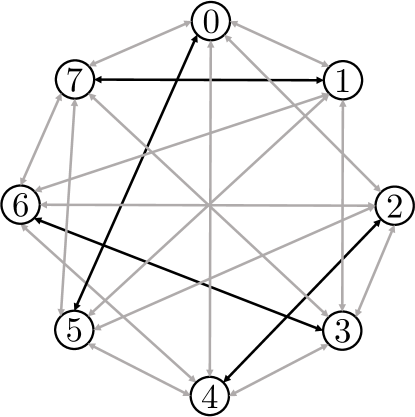
Figure 9: Graph representation of connections between the symmetry subspaces where pairs {2,4}, {0,5}, {6,3}, {7,1} correspond to the top and bottom sections of the octants where each unstable RPO lies. The intensity of each connection is related to the probability of the trajectory transitioning to another chart. The probability of staying in the same chart (not included in this depiction) is $\sim 94\%$, . Darker lines correspond to forward and reverse probabilities of $\sim 5\%$. Lighter lines correspond to forward and reverse probabilities of $\leq 1\%$.

Here we discuss the detailed operations for evolving trajectories in the fundamental chart with the NODE models. Fig. 10a summarizes the methodology for evolving in time. An initial condition in the fundamental space is first encoded and projected with $\hat{U}$ to obtain $h(t)$. Then the NODE maps a trajectory forward $T$ time units to yield $h_{\text{temp}}(t+T)$ (note the indicator does not change in this step). We select $T=\tau$. After this, we perform the appropriate symmetry operations, detailed below, to find $h_{r}(t+T)$ and update the new indicator $\mathcal{I}(t+T)$. This is repeated to continue evolving forward in time. In Fig. 10b we present the method for performing these symmetry operations.

There are two main steps in applying the symmetry operations: 1) determining $\mathcal{I}$ from $h_{\text{temp}}$, and 2) getting the values of $h_{r}(t+T)$ and $\mathcal{I}(t+T)$. Step 1 is simply a classification problem where we wish to find a function that classifies new values of $h_{\text{temp}}$ as either lying within or outside the fundamental domain. In Floryan & Graham [15] this was performed by identifying the nearest neighbor of the training data in the manifold coordinates and classifying $h_{\text{temp}}$ with the same label. However, any classification technique can work – for example, support vector machines (SVM) [34] also worked well at this task. In the case of our specific problem, we found the fastest method was to map $h_{\text{temp}}$ to the ambient space $\omega_{\text{temp}}$ at every step and calculate $\hat{\omega}_{R}(0,1)$, $\hat{\omega}_{I}(0,1)$, $\hat{\omega}_{I}(0,2)$ to verify if $h_{\text{temp}}$ lies in the fundamental space. Step 2 involves updating the manifold coordinates to get $h_{r}(t+T)$. If the indicator changes, symmetries are factored out with $\mathcal{I}(t+T)$ and the snapshot is encoded to get the new $h_{r}(t+T)$. If the indicator stays the same $h_{r}(t+T)=h_{\text{temp}}(t+T)$ and $\mathcal{I}(t+T)=\mathcal{I}(t)$.

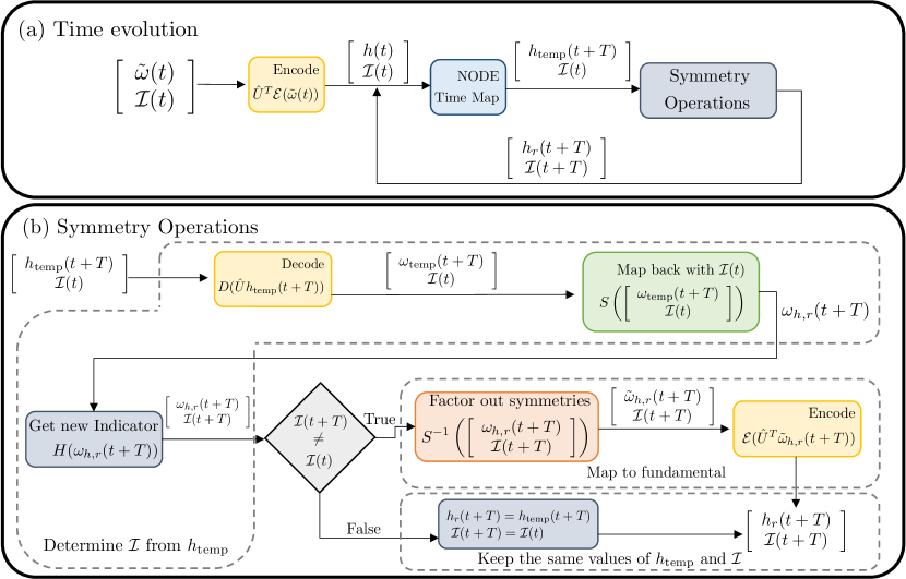
Figure 10: (a) Time evolution of $h(t)$ with NODE and (b) symmetry operation check to map back to fundamental space if needed.

III.4 Time evolution of phase with neural ODEs

We also wish to time-evolve the phase $\phi_{x}(t)$. The dynamics of the phase only depend upon the fundamental-chart vorticity pattern $h$ and the indicator $\mathcal{I}$, so we can describe them with

$$\dfrac{d\phi_{x}}{dt}=g_{\mathcal{I}}(\mathcal{I})g_{\phi}(h;\theta_{\phi}).$$ (14)

The term $g_{\mathcal{I}}(\mathcal{I})$ equals 1 if an even number of discrete operations map $h$ back to the fundamental space, or -1 if an odd number of discrete operations map $h$ back to the fundamental space. To understand how the signs of Equation 14 change consider the effect of discrete symmetry operations on the phase calculation $\phi_{x}=\operatorname{atan}2\left\{\hat{\omega}_{I}(1,0),\hat{\omega}_{R}(1,0)\right\}$. Applying a discrete symmetry operation on a snapshot changes the phase variable to either

$$\phi_{x,\mathscr{S}}=\mathscr{S}\phi_{x}=\operatorname{atan}2\left\{\hat{\omega}_{I}(1,0),-\hat{\omega}_{R}(1,0)\right\}=\pi-\phi_{x},$$ (15)

or

$$\phi_{x,\mathscr{R}}=\mathscr{R}\phi_{x}=\operatorname{atan}2\left\{-\hat{\omega}_{I}(1,0),\hat{\omega}_{R}(1,0)\right\}=-\phi_{x}.$$ (16)

Then, by simply taking the time derivative, we see that $d\phi_{x,\mathscr{S}}/dt=-d\phi_{x}/dt$ and $d\phi_{x,\mathscr{R}}/dt=-d\phi_{x}/dt$. Hence the operation of a discrete symmetry (rotation and shift-reflect) changes the sign. Now, we train $g_{\phi}$ by fixing the NODE $g_{h}$ to evolve $h$ forward in time, and use Equation 14 to make predictions $\phi_{x,r}$. We update the parameters of $g_{\phi}$ to minimize the loss

$$\mathcal{L}_{\phi,\text{NODE}}\left(\phi_{x};\theta_{\phi}\right)=\left\langle\left\|\phi_{x}(t+\tau)-\phi_{x,r}(t+\tau)\right\|_{2}^{2}\right\rangle,$$ (17)

and refer to Table 2 for details on the NODE architecture.

Table 2: Neural network layer dimensions and activations used in each layer. Sigmoid functions are denoted ‘S’. Number of linear layers $W_{i}$ can be varied.

$$\begin{array}[]{lccc}\hline\cr\hline\cr&\text{ Function }&\text{ Shape }&\text{ Activation }\\ \hline\cr\text{ Encoder }&E&1024:2048:256:40&\text{ ReLU:ReLU:Linear }\\ \text{ Decoder }&D&40:256:2048:1024&\text{ ReLU:ReLU:Linear }\\ \text{ Linear Net }&\mathcal{W}=W_{1}W_{2}...&40:40&\text{Linear }\\ \text{ Pattern NODE }&g_{h}&d_{m}:500:500:500:d_{m}&\text{ S:S:S:Linear }\\ \text{ Phase NODE }&g_{\phi}&d_{m}:500:500:500:1&\text{ S:S:S:Linear }\\ \hline\cr\hline\cr\end{array}$$

IV Results

We present results for the chaotic case $\mathrm{Re}=14.4$, whose trajectories sample all eight charts introduced above. First we illustrate the effect of training data size on the autoencoder performance when considering the fundamental chart data, as opposed to using the original and phase-aligned data. These results are shown in Section IV.1.1. We then use IRMAE-WD to estimate the minimal dimension needed to represent the data. We summarize these results in Section IV.1.2. The time evolution model performance results are shown in Section IV.2. Here we confirm the equivariance of the model, (Section IV.2.1) then show the performance for short-time tracking, long-time statistics, and phase evolution (Sections IV.2.2, IV.2.3, and IV.2.4 respectively).

IV.1 Dimension reduction with IRMAE-WD

To train our IRMAE-WD models we minimize $\mathcal{L}$ via stochastic gradient descent. Following Zeng et al. [12], we use the AdamW optimizer, which decouples weight decay from the adaptive gradient update and helps avoid the issue of weights with larger gradient amplitudes being regularized disproportionately, as observed in Adam [35]. All models were trained for a total of 1000 epochs and with a learning rate of $10^{-3}$. We consider $10^{5}$ snapshots of the original data ($\omega$), the phase-aligned data ($\omega_{l}$), and the data mapped to the fundamental space ($\tilde{\omega}$) separated by $\tau=0.5$ time units.

Before training the AEs, the mean is subtracted and the data is divided by its standard deviation. Three models are trained for each case of varying number of linear layers $L=0,4,6,8,10$ and weight decay values of $\lambda=10^{-4},10^{-6},10^{-8}$ for a total of 45 models for the $\omega$, $\omega_{l}$, and $\tilde{\omega}$ cases. For all of the networks discussed in this work, we use a $80/20$ split of the data for training and testing respectively. We select $d_{z}=40$, which is significantly higher than the dimension expected based on our previous work [10].

IV.1.1 Effect of training data size on performance

A major benefit of mapping our data to the fundamental chart is that it results in eightfold denser sampling within that chart, as shown in Fig. 6. We also see that all the data is in a much smaller part of state space, and only that part of state space needs to be represented. As such, in this section, we test if this increased density allows us to use less data for training AEs. We factor out the symmetries of our system as discussed in Section III.1 and train IRMAE-WD models for the case of $L=4$ and $\lambda=10^{-4}$. In Fig. 11 we show the test MSE of the IRMAE-WD models as we vary the amount of data for three cases: the original data ($\omega$), the phase-aligned data ($\omega_{l}$), and the data mapped to the fundamental space ($\tilde{\omega}$). In all cases, we use the same $20,000$ test snapshots to calculate the MSE, train 3 models at each training data size, and reduce to a dimension of $d_{z}=40$. Notice that here we do not project to a lower dimension; that will be done below. The purpose here is not to map to the minimal dimension, but to study the effect of data size on training.

As can be seen in Fig. 11, removing phase results in an order of magnitude improvement in the MSE over the original data, and mapping to the fundamental results in nearly another order of magnitude improvement in the MSE over the phase-aligned data. Thus, this drastic improvement in performance allows us to use far less data. For example, 800 snapshots in the fundamental space performs nearly as well as $80,000$ snapshots in the original space. Similarly, $8,000$ snapshots in the fundamental case outperforms $80,000$ snapshots in the phase-aligned case. Now that we have shown the effect of the number of snapshots on performance we use $80,000$ snapshots for the remaining studies.

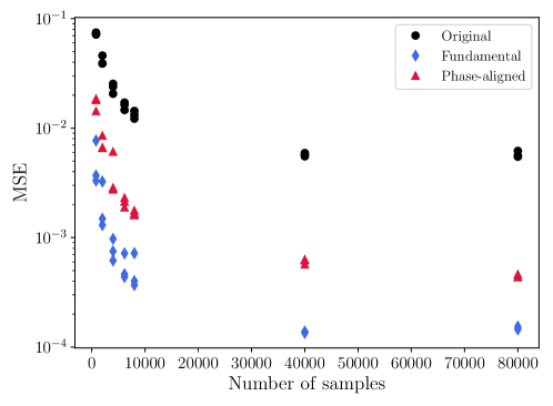
Figure 11: MSE vs number of data size used for training IRMAE-WD corresponding to a test data of 20,000 samples for $\text{Re}=14.4$. The parameters used are $L=4$ and $\lambda=10^{-4}$ and three trials are considered for each case. The data is reduced to a dimension of $d_{z}=40$.

IV.1.2 Effect on dimension estimates with varying linear layers and weight decay

Here we study the effects on the dimension estimates when varying $L$ and $\lambda$ for the original, phase-aligned, and fundamental case. As discussed in Section III.2 we perform SVD on the covariance matrix of the encoded data $ZZ^{T}$ to obtain $U$ and truncate to obtain $h=\hat{U}^{T}z$. Zeng et al. [12] showed that structuring an autoencoder with linear layers and using weight decay causes the latent space to become low-dimensional through training. In Fig. 12, we show the evolution of these singular values through training. As the model trains for longer times, the trailing singular values tend towards zero. These can be truncated without any loss of information. For most cases, this drop is drastic ($\sim 10$ orders of magnitude) and a threshold can be defined to select how many singular values to keep (i.e. to select the number of dimensions).

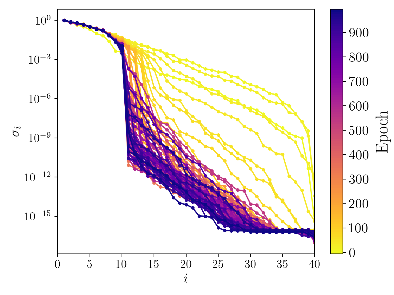
Figure 12: Evolution of singular values of the covariance matrix of the encoded test data $ZZ^{T}$ during training of an IRMAE-WD model with $L=4$ and $\lambda=10^{-4}$. Here the drop happens at $d_{h}=10$.

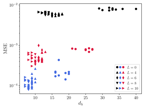
Figure 13: MSE vs dimension $d_{h}$ given by the spectral gap of the singular values for the original (black), phase-aligned (red), and fundamental chart (blue) cases. Each case contains three trials of combinations of parameters $L=0,4,6,8,10$ and $\lambda=10^{-4},10^{-6},10^{-8}$.

In Fig. 13 we plot the estimate of dimension for the original (black), phase-aligned (red), and fundamental chart (blue) data as we vary the number of linear layers $L$ and the weight decay parameter $\lambda$. For each case, there are two clear clusters – the cluster with higher dimension corresponds to $L=0$ and the other cluster has linear layers, $L>0$.This happens because in the absence of linear layers there is no mechanism to drive the rank to a minimal value. When we factor out symmetries the dimension estimates become less spread with ranges of $d_{h}=7-10$ for fundamental, $d_{h}=8-13$ for phase-aligned, and $d_{h}=11-18$ for original. This narrowing of the distribution likely happens due to the dense coverage of the state space in the fundamental chart, which better captures the shape of the manifold. The dimension estimate range from the fundamental chart is in good agreement with our previous observations of $d_{h}=9$ in [10]. In the following analysis we select a conservative estimate of the dimension which appears to be $d_{h}=10$ from the fundamental chart data.

IV.2 Time evolution

To learn our NODE models we first train $g_{h}$ by minimizing Equation 13 ($\mathcal{L}_{\text{NODE}}$) and then we fix $g_{h}$ and train $g_{\phi}$ by minimizing Equation 14 ($\mathcal{L}_{\phi,\text{NODE}}$) via the Adam optimizer. We train for a total of 40000 epochs and a learning rate scheduler that drops from $10^{-3}$ to $10^{-4}$ at epoch number 13334 (1/3 into training) and from $10^{-4}$ to $10^{-5}$ at epoch number 26667 (2/3 into training). As previously discussed we use $\tau=0.5$ which ensures the trajectory spends some time steps in an overlap region as it moves from chart to chart, so we can learn the dynamics there.

IV.2.1 Equivariance

The results we obtain with this framework should be equivariant with respect to initial conditions. This means that after we apply any of the symmetry operations described above to an initial condition, the resulting trajectory from the original initial condition and the new initial condition must be equivalent up to this symmetry operation. Here we show that our methodology retains equivariance. We select the IRMAE-WD models with the lowest MSEs at a dimension of $d_{h}=10$, which is a conservative dimension estimates for the fundamental case, for both the phase-aligned and fundamental model. We then sample 1000 initial conditions separated by 10 time units such that we cover different regions of state space. For every initial condition, we apply all the discrete symmetry operations in the original Fourier space, mapping the data into every octant. Then we evolve these initial conditions forward 1000 time units with the DManD model, with and without symmetry charting. To test for equivariance, we compute the trajectory error $TE$ between predicted trajectories as follows

$$TE(t)=\frac{1}{100\times 7}\sum_{i=1}^{100}\sum_{j=1}^{7}\|\tilde{\omega}_{i,j}(t)-\tilde{\omega}_{i,j=0}(t)\|,$$ (18)

where $i$ corresponds to the trajectory number, and $j$ to the initial chart (i.e. $j=0$ corresponds to the original initial condition of the $i$th trajectory). Fig. 14 presents this error through time for our symmetry charting method (Fundamental) and for models with only phase-alignment.

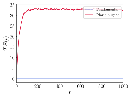
Figure 14: $TE(t)$ vs $t$ for Fundamental and Phase-aligned case where $TE(t)$ corresponds to the error calculation between predicted NODE trajectories, from a model with $d_{h}=10$, from initial conditions that are related by symmetry transformations.

As expected, the time integration from the model trained in the fundamental space satisfies equivariance perfectly with a $TE=0$. The phase-aligned curve does not satisfy equivariance, and we see that trajectories diverge fairly quickly.

A more severe consequence of not enforcing the discrete symmetries can be seen in trajectory predictions. Fig. 15 depicts $\|\omega(t)\|$ vs $t$ for the true data (shown in black) and the time integration of initial conditions starting in different charts (red – $\mathcal{I}=0$, blue – $\mathcal{I}=1$, and green – $\mathcal{I}=2$) for both fundamental (a) and phase-aligned cases (b). In all cases, the predicted trajectories diverge from the true trajectory after some time – this is expected for a chaotic system, as explore further in Section IV.2.2. However, the symmetry-charted predictions in Fig. 15(a) exhibit excellent short-time tracking and captures the bursting event that happens around $t=100$. At longer times, the prediction is not quantitatively accurate but still captures the alternation between quiescent and bursting intervals observed in the true data. By contrast, the predictions for the phase-aligned model, Fig. 15(b), deviate quickly from the true data, and furthermore do not even exhibit intermittency between quiescent and bursting dynamics – they stay in a bursting regime. Thus the models that do not account for the discrete symmetries do not capture the dynamics correctly, even at a qualitative level. These results reinforce the major advantage of properly accounting for symmetries, as the symmetry charting method does.

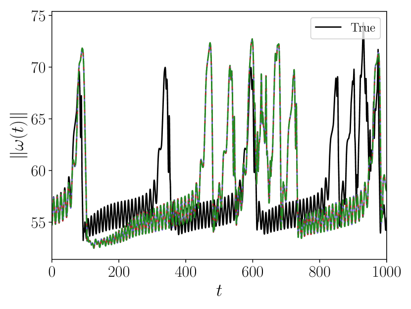
(a)

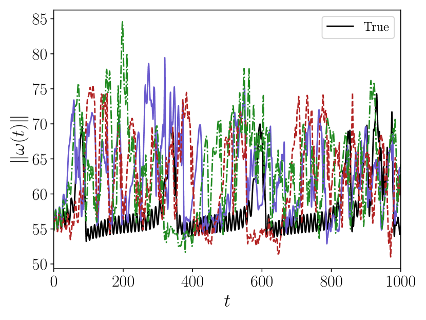
(b)

Figure 15: $\|\omega(t)\|$ vs time for initial conditions integrated with the (a) Fundamental and (b) Phase aligned NODE model for $d_{h}=10$. Colors correspond to initial conditions starting in different fundamental domains (red – $\mathcal{I}=0$, blue – $\mathcal{I}=1$, and green – $\mathcal{I}=2$). In (a), all the different-colored trajectories coincide.

IV.2.2 Short-time predictions

In this section, we focus on short-time trajectory predictions. The Lyapunov time $t_{L}$ for this system is approximately $t_{L}\approx 20$ [36]. We take initial conditions of $h(t)$ and evolve for $100$ time units. These are then decoded and compared with the true vorticity snapshots. We consider trajectories with initial conditions starting in the quiescent as well as in the bursting regions. The dynamics at $\text{Re}=14.4$ are characterized by quiescent intervals where the trajectories are close to RPOs (which are now unstable), punctuated by heteroclinic-like excursions (bursting) between the RPOs, which are indicated by the intermittent increases of $\|\omega(t)\|$ as observed in Fig. 3(a). The nature of the intermittency of the data makes it challenging to assign either bursting or quiescent labels. To split the initial conditions as quiescent or bursting we use the algorithm discussed in [10].

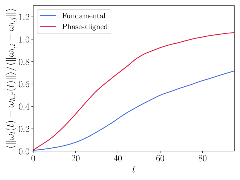
(a)

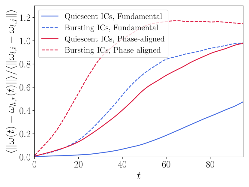
(b)

Figure 16: Difference between true vorticity evolution and vorticity evolution obtained from the Fundamental and Phase aligned NODEs from $h(t)$ of $d_{h}=10$, where (a) corresponds to averages over all initial conditions, and (b) corresponds to averages taken over bursting and quiescent initial conditions.

We first show in Fig. 16(a) the ensemble-averaged prediction error as a function of time for $10^{4}$ initial conditions. We use the same models as in the previous section which corresponds to $d_{h}=10$ for both fundamental and phase-aligned case. The comparison is done with true phase-aligned data, so after obtaining the prediction from the fundamental case we use the indicators to include the symmetries. The error is normalized with random differences of the true data, where $i$ and $j$ correspond to different snapshots. With this normalization, when the curves approach 1 this means that on average the distance between the model and the true data is the same as if we selected random points from the true data. The DManD models using symmetry charting significantly outperform the phase-aligned DManD models. This agrees with Fig. 15 as discussed above. Similar improvement is observed in Fig. 16(b), and can be attributed to the organized (near-RPO) nature of the dynamics in the quiescent region. Also, the dynamics spend more time in this area, so there is more data for the autoencoder to train on.

IV.2.3 Long-time predictions

Now that we demonstrated the short-time predictive capabilities of the model, we next turn to the ability of the model to reconstruct the long-time statistics of the attractor. For this comparison, we sample $2\times 10^{4}$ time units of data every $0.5$ time units for the DNS and the DManD models. Fig. 17 shows the joint probability density function (PDF) of $\text{Re}[a_{0,1}(t)]$ and $\text{Im}[a_{0,1}(t)]$ for true and predicted data from the models with $d_{h}=10$ for the fundamental and phase-aligned case. The true joint PDF (Fig. 17(a)) and the symmetry charting fundamental joint PDF (Fig. 17(b)) are in excellent agreement. These PDFs both show a strong, equal preference for trajectories to shadow the four unstable RPOs, and lower probabilities between them where the bursting transitions of the RPO regions occur. In contrast, the joint PDF for the phase-aligned model (Fig. 17(c)) shows that the model samples the space before falling onto an unphysical stable RPO (bright closed curve) near one of the true system’s unstable RPOs. Clearly, in this case, the phase-aligned model fails to capture the system’s true dynamics.

Another important quantity to consider is the ability of the models to capture the energy balance of the system. In Fig. 18 we show the joint PDF of $I$ and $D$ for the DNS and the same models. Again, the model trained in the fundamental space closely matches the joint PDF of the true data. The phase-aligned model both underestimates the energy associated with the high probability RPOs, and overestimates the energy associated with the low probability high power input and dissipation events.

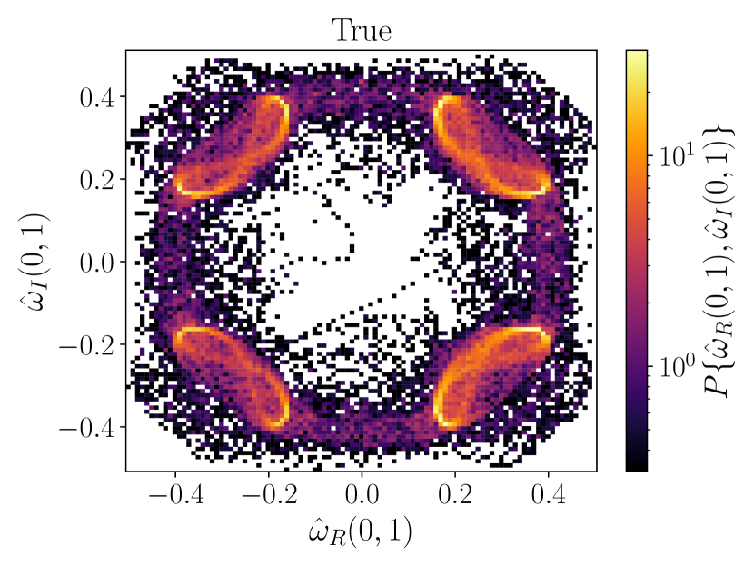
(a)

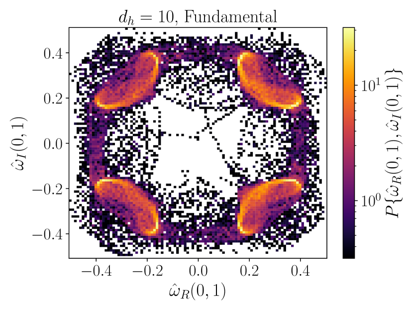
(b)

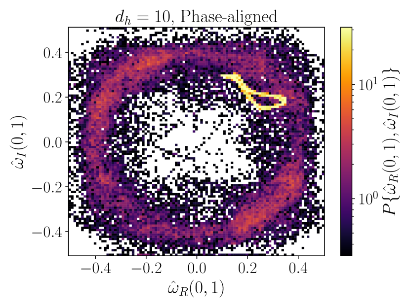
(c)

Figure 17: Joint PDFs of $\hat{\omega}_{R}(0,1)$-$\hat{\omega}_{I}(0,1)$ of (a) true, and predicted data corresponding to dimension $d_{h}=10$ from the (b) Fundamental and (c) Phase-aligned models.

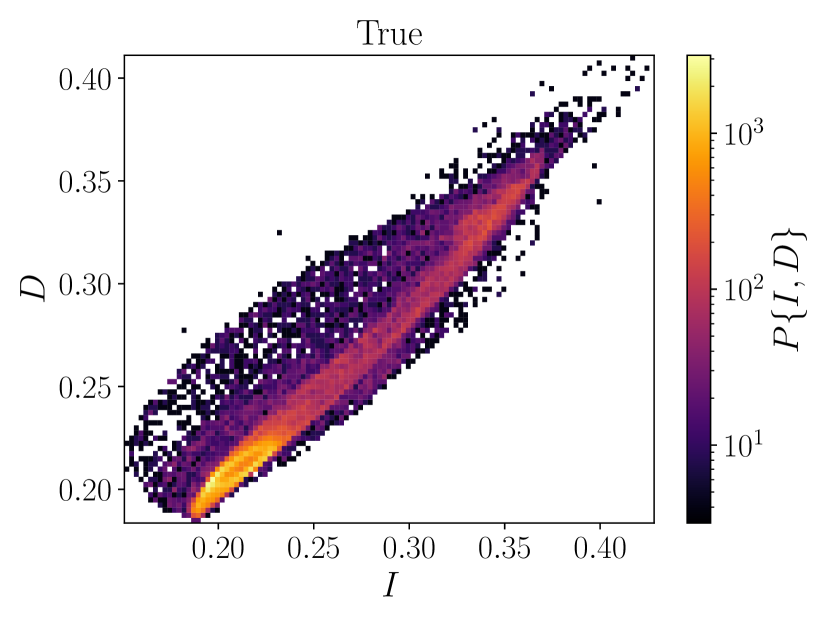
(a)

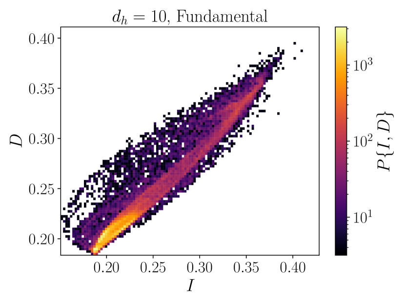
(b)

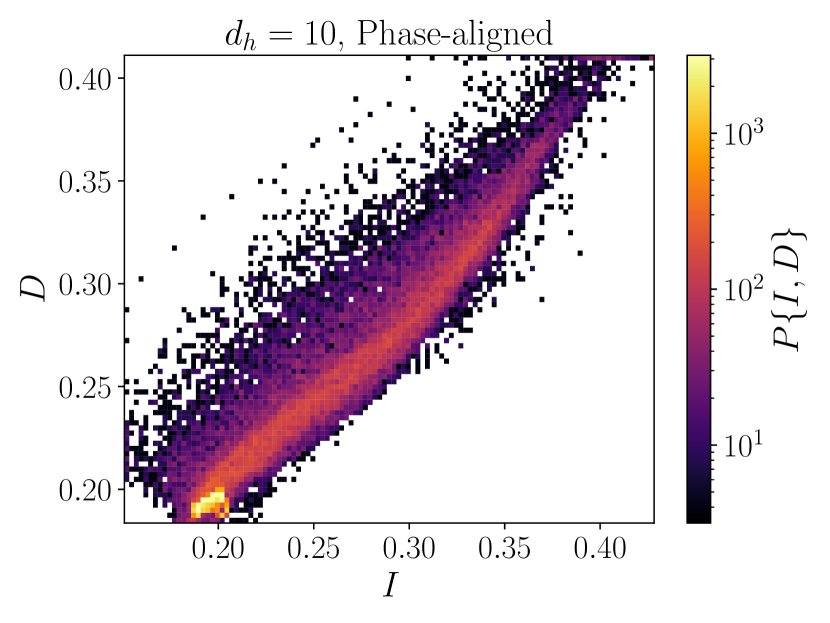
(c)

Figure 18: Joint PDFs of $I$-$D$ of (a) true, and predicted data corresponding to dimension $d_{h}=10$ from the (b) Fundamental and (c) Phase-aligned models.

IV.2.4 Phase variable prediction

To complete the dynamical picture we predict the phase evolution as given by Equation 14. We compare the models to the true data by calculating the mean squared displacement (MSD) of the phase,

$$\mbox{MSD}(t)=\langle(\phi_{x}(t)-\phi_{x}(0))^{2}\rangle$$ (19)

as was done in our previous work [10]. Due to the bursting region, where the direction of phase evolution is essentially randomly reset, at long times the phase $\phi_{x}$ exhibits random-walk behavior, which the MSD reflects. We take $420$ initial conditions separated by $15$ time units and use the models of $d_{h}=10$ to predict $\phi_{x}(t)$ and calculate the MSD. This is done for the fundamental and phase-aligned models.

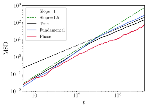
Figure 19: MSD of $\phi_{x}(t)$ corresponding to models with dimension $d_{h}=10$.

Fig. 19 shows the evolution of MSD of true and predicted data. Here the black solid line corresponds to the true data, and the black and green dashed lines serve as references with slopes of $1$ and $1.5$ respectively. There is a change from superdiffusive ($MSD\sim t^{1.5}$) to diffusive ($MSD\sim t$) scaling around $t\approx 200$, which corresponds to the mean duration of the quiescent intervals: i.e., to the average time the trajectories travel along the RPOs before bursting. The fundamental chart model accurately captures both the change in slope and the timing of this change in slope. However, the curve of the phase-aligned model fails to match the true MSD at long times. This happens because the phase-aligned model is unable to predict $h(t)$ correctly at long times as observed in Fig. 15(b), hence resulting in poor predictions for $\phi_{x}(t)$.

V Conclusion

Symmetries appear naturally in dynamical systems and we show here that correctly accounting for them dramatically improves the performance of data-driven models for time evolution on an invariant manifold. In this work, we introduce a method that we call symmetry charting and apply it to Kolmogorov flow in a chaotic regime of $\text{Re}=14.4$. This symmetry charting method factors out symmetries so we can train ROMs in a fundamental chart and ensure equivariant trajectories – we are essentially learning coordinates and dynamics on one region (chart) of the invariant manifold for the long-time dynamics rather than having to learn these for the entire manifold. To do so, we first factor out the symmetries by identifying a set of indicators that differentiate the set of discrete symmetries for the system. Here, Fourier coefficients serve this purpose; we found that the signs of specific Fourier modes could uniquely identify all discrete symmetry operations. We then use IRMAE-WD, an autoencoder architecture that tends to drive the rank of the latent space covariance of the data to a minimum, to find a low-dimensional representation of the data. This method overcomes the need to sweep over latent space dimensions. We observe that factoring out symmetries improves the MSE of the reconstruction as well as the dimension estimates and robustness to IRMAE-WD hyperparameters. When considering the original data (i.e. no symmetries factored out) and the phase-aligned data (only continuous symmetry factored out) the MSE is higher and the range of dimension estimates is wider. We also note that the dimension estimate range in the fundamental chart agrees well with the dimension found in our previous work for the same system [10]. We then train a NODE with latent space of dimension $d_{h}=10$ for both phase-aligned and fundamental space data. This dimension is the upper bound of the dimension estimate obtained for the fundamental chart data. The resulting models using symmetry charting to map to the fundamental space accurately reconstructed the DNS at both short and long times. In contrast, the phase-aligned model quickly landed on an unphysical stable RPO leading to poor reconstruction of the dynamics.

The approach described here is essentially a version of the “CANDyMan” (Charts and Atlases for Nonlinear Data-driven Dynamics on Manifolds) approach described in [15, 16]. As shown on those studies, learning charts and atlases to develop local manifold representations and dynamical models can improve performance for systems with complex dynamics. There, however, the charts were found by clustering; here that step is bypassed by using a priori knowledge, about the system, namely its symmetries. The methodology presented in this work can be applied to other dynamical systems with rich symmetries by identifying the corresponding indicators. Future directions for symmetry charting and CANDyMan include applications such as control in systems with symmetry (cf. [20]) as well as development of hierarchical methods where the fundamental chart identified by symmetry can be further subdivided using a cluster algorithm or a chart autoencoder [37].

- [1] Prem A Srinivasan, L Guastoni, Hossein Azizpour, Philipp Schlatter, and Ricardo Vinuesa. Predictions of turbulent shear flows using deep neural networks. Physical Review Fluids, 4(5):054603, 2019.
- [2] Jacob Page, Michael P Brenner, and Rich R Kerswell. Revealing the state space of turbulence using machine learning. Physical Review Fluids, 6(3):034402, 2021.
- [3] Nguyen Anh Khoa Doan, Wolfgang Polifke, and Luca Magri. Auto-encoded reservoir computing for turbulence learning. In International Conference on Computational Science, pages 344–351. Springer, 2021.
- [4] Taichi Nakamura, Kai Fukami, Kazuto Hasegawa, Yusuke Nabae, and Koji Fukagata. Convolutional neural network and long short-term memory based reduced order surrogate for minimal turbulent channel flow. Physics of Fluids, 33(2):025116, 2021.
- [5] Ciprian Foias, O Manley, and Roger Temam. Modelling of the interaction of small and large eddies in two dimensional turbulent flows. ESAIM: Mathematical Modelling and Numerical Analysis, 22(1):93–118, 1988.
- [6] R Temam. Do inertial manifolds apply to turbulence? Physica D: Nonlinear Phenomena, 37(1-3):146–152, 1989.
- [7] Sergey Zelik. Attractors. Then and now. arXiv preprint arXiv:2208.12101, 2022.
- [8] Alec J Linot and Michael D Graham. Deep learning to discover and predict dynamics on an inertial manifold. Physical Review E, 101(6):062209, 2020.
- [9] Alec J Linot and Michael D Graham. Data-driven reduced-order modeling of spatiotemporal chaos with neural ordinary differential equations. Chaos: An Interdisciplinary Journal of Nonlinear Science, 32(7):073110, 2022.
- [10] Carlos E Pérez De Jesús and Michael D Graham. Data-driven low-dimensional dynamic model of Kolmogorov flow. Physical Review Fluids, 8(4):044402, 2023.
- [11] Alec J Linot and Michael D Graham. Dynamics of a data-driven low-dimensional model of turbulent minimal Couette flow. arXiv preprint arXiv:2301.04638, 2023.
- [12] Kevin Zeng, Carlos E Pérez De Jesús, Andrew J Fox, and Michael D Graham. Autoencoders for discovering manifold dimension and coordinates in data from complex dynamical systems. arXiv preprint arXiv:2305.01090, 2023.
- [13] Li Jing, Jure Zbontar, et al. Implicit rank-minimizing autoencoder. Advances in Neural Information Processing Systems, 33:14736–14746, 2020.
- [14] John M Lee. Smooth manifolds. In Introduction to smooth manifolds, pages 1–31. Springer, 2013.
- [15] Daniel Floryan and Michael D Graham. Data-driven discovery of intrinsic dynamics. Nature Machine Intelligence, 4(12):1113–1120, 2022.
- [16] Andrew J Fox, C Ricardo Constante-Amores, and Michael D Graham. Predicting extreme events in a data-driven model of turbulent shear flow using an atlas of charts. Physical Review Fluids, 8(9):094401, 2023.
- [17] Simon Kneer, Taraneh Sayadi, Denis Sipp, Peter Schmid, and Georgios Rigas. Symmetry-Aware Autoencoders: s-PCA and s-nlPCA. arXiv preprint arXiv:2111.02893, 2021.
- [18] Rick Miranda and Emily Stone. The proto-Lorenz system. Physics Letters A, 178(1-2):105–113, 1993.
- [19] Nazmi Burak Budanur and Predrag Cvitanović. Unstable manifolds of relative periodic orbits in the symmetry-reduced state space of the Kuramoto–Sivashinsky system. Journal of Statistical Physics, 167(3-4):636–655, 2017.
- [20] Kevin Zeng and Michael D Graham. Symmetry reduction for deep reinforcement learning active control of chaotic spatiotemporal dynamics. Physical Review E, 104(1):014210, 2021.
- [21] Christopher J Crowley, Joshua L Pughe-Sanford, Wesley Toler, Michael C Krygier, Roman O Grigoriev, and Michael F Schatz. Turbulence tracks recurrent solutions. Proceedings of the National Academy of Sciences, 119(34):e2120665119, 2022.
- [22] D Armbruster, B Nicolaenko, N Smaoui, and Pascal Chossat. Symmetries and dynamics for 2-D Navier-Stokes flow. Physica D: Nonlinear Phenomena, 95(1):81–93, 1996.
- [23] Ricky TQ Chen, Yulia Rubanova, Jesse Bettencourt, and David K Duvenaud. Neural ordinary differential equations. Advances in neural information processing systems, 31, 2018.
- [24] Gary J Chandler and Rich R Kerswell. Invariant recurrent solutions embedded in a turbulent two-dimensional Kolmogorov flow. Journal of Fluid Mechanics, 722:554–595, 2013.
- [25] VI Iudovich. Example of the generation of a secondary stationary or periodic flow when there is loss of stability of the laminar flow of a viscous incompressible fluid. Journal of Applied Mathematics and Mechanics, 29(3):527–544, 1965.
- [26] LD Meshalkin and Ia G Sinai. Investigation of the stability of a stationary solution of a system of equations for the plane movement of an incompressible viscous liquid. Journal of Applied Mathematics and Mechanics, 25(6):1700–1705, 1961.
- [27] JSA Green. Two-dimensional turbulence near the viscous limit. Journal of Fluid Mechanics, 62(2):273–287, 1974.
- [28] André Thess. Instabilities in two-dimensional spatially periodic flows. Part I: Kolmogorov flow. Physics of Fluids A: Fluid Dynamics, 4(7):1385–1395, 1992.
- [29] Peter Bartello and Tom Warn. Self-similarity of decaying two-dimensional turbulence. Journal of Fluid Mechanics, 326:357–372, 1996.
- [30] Nazmi Burak Budanur and P. Cvitanović. Unstable Manifolds of Relative Periodic Orbits in the Symmetry-Reduced State Space of the Kuramoto–Sivashinsky System. Journal of Statistical Physics, 167(3-4):636–655, 2017.
- [31] Nazmi Burak Budanur, Daniel Borrero-Echeverry, and Predrag Cvitanović. Periodic orbit analysis of a system with continuous symmetry—A tutorial. Chaos: An Interdisciplinary Journal of Nonlinear Science, 25(7):073112, 2015.
- [32] Nazmi Burak Budanur, Predrag Cvitanović, Ruslan L Davidchack, and Evangelos Siminos. Reduction of SO (2) symmetry for spatially extended dynamical systems. Physical review letters, 114(8):084102, 2015.
- [33] Alec J Linot, Joshua W Burby, Qi Tang, Prasanna Balaprakash, Michael D Graham, and Romit Maulik. Stabilized neural ordinary differential equations for long-time forecasting of dynamical systems. Journal of Computational Physics, 474:111838, 2023.
- [34] Bernhard E Boser, Isabelle M Guyon, and Vladimir N Vapnik. A training algorithm for optimal margin classifiers. In Proceedings of the fifth annual workshop on Computational learning theory, pages 144–152, 1992.
- [35] Ilya Loshchilov and Frank Hutter. Decoupled weight decay regularization. arXiv preprint arXiv:1711.05101, 2017.
- [36] Masanobu Inubushi, Miki U Kobayashi, Shin-ichi Takehiro, and Michio Yamada. Covariant Lyapunov analysis of chaotic Kolmogorov flows. Physical Review E, 85(1):016331, 2012.
- [37] Stefan Schonscheck, Jie Chen, and Rongjie Lai. Chart Auto-Encoders for Manifold Structured Data. arXiv, 2019.