Targeted Machine Learning for Average Causal Effect Estimation Using the Front-Door Functional

Abstract

Evaluating the average causal effect (ACE) of a treatment on an outcome often involves overcoming the challenges posed by confounding factors in observational studies. A traditional approach uses the back-door criterion, seeking adjustment sets to block confounding paths between treatment and outcome. However, this method struggles with unmeasured confounders. As an alternative, the front-door criterion offers a solution, even in the presence of unmeasured confounders between treatment and outcome. This method relies on identifying mediators that are not directly affected by these confounders and that completely mediate the treatment’s effect. Here, we introduce novel estimation strategies for the front-door criterion based on the targeted minimum loss-based estimation theory. Our estimators work across diverse scenarios, handling binary, continuous, and multivariate mediators. They leverage data-adaptive machine learning algorithms, minimizing assumptions and ensuring key statistical properties like asymptotic linearity, double-robustness, efficiency, and valid estimates within the target parameter space. We establish conditions under which the nuisance functional estimations ensure the $n^{1/2}$-consistency of ACE estimators. Our numerical experiments show the favorable finite sample performance of the proposed estimators. We demonstrate the applicability of these estimators to analyze the effect of early stage academic performance on future yearly income using data from the Finnish Social Science Data Archive.

1 Introduction

The average causal effect (ACE) is a key parameter for quantifying the cause-effect relationship between a treatment and a response variable. This parameter measures the difference in the average of potential outcomes that would have occurred if the treatment was administered compared to if it was not. One approach commonly used to identify the ACE is the back-door adjustment, which involves identifying a set of variables that would block all the confounding paths between the treatment and the outcome (Pearl, 2009). The resulting back-door adjustment functional is also known as g-formula (Robins, 1986; Hahn, 1998) and enjoys an inverse probability of treatment weighted (IPTW) representation (Hirano et al., 2003). There exists a rich literature on how to estimate the back-door adjustment functional with proposals ranging from simple plug-in or IPTW estimators to more complicated estimators such as augmented IPTW or targeted minimum loss based estimators (TMLEs), which are obtained using semiparametric efficiency theory (Bickel et al., 1993; van der Vaart, 2000; Tsiatis, 2007; Robins et al., 1994a; van der Laan et al., 2011; Chernozhukov et al., 2017).

Finding a sufficient back-door adjustment set in observational studies can be challenging as there are often unmeasured factors impacting the causal relationship between the treatment and outcome. Various approaches are commonly employed to address this issue. These include the use of instrumental variables (Balke and Pearl, 1994), conducting sensitivity analysis (Robins et al., 2000; Scharfstein et al., 2021), or deriving nonparametric bounds (Manski, 1990). An alternative strategy involves the use of directed acyclic graphs (DAGs) with hidden/unmeasured variables to encode independence restrictions between counterfactual and observed variables within a nonparametric model (Tian and Pearl, 2002; Richardson and Robins, 2013). This graphical approach has led to the development of sound and complete algorithms for identifying causal parameters based on the observed data distribution (Shpitser and Pearl, 2006; Huang and Valtorta, 2006; Richardson et al., 2017; Bhattacharya et al., 2022). These identification algorithms take a hidden variable DAG as input and determine whether the ACE can be identified as a function of a joint distribution defined solely over observed variables. If identification is possible, the algorithm provides an identifying functional that captures the ACE.

The front-door model is perhaps the simplest example of a DAG with unmeasured confounders where no valid back-door adjustment set exists, yet the causal effect can still be identifiable (Pearl, 1995a). In this model, the ACE identification relies on measuring one or more mediating variables that satisfy two conditions: (i) the treatment-mediators and mediators-outcome relations are free from unmeasured confounders, and (ii) the effect of treatment on outcome is fully mediated through such variables. Empirical evaluations suggest that employing front-door adjustment can yield reasonable estimates of causal effects in real-world scenarios where the presence of unmeasured confounding between treatment and outcome is expected (Glynn and Kashin, 2013, 2018; Bellemare et al., 2019; Bhattacharya and Nabi, 2022).

A nonparametric efficient estimator for the front-door functional was proposed by Fulcher et al. (2019). The proposed estimator is built based on parametric working models for three key nuisance parameters: the conditional mean outcome, the conditional distribution of the mediator(s), and the conditional probability of the treatment. While the estimator relies on parametric working models, it enjoys a double-robustness property. While this estimator marked an important contribution to the literature on estimation of the front-door functional, several critical considerations, both technical and practical, remain.

First, the work by Fulcher et al. (2019) focuses on estimators of the front-door functional built using simple nuisance estimates based on parametric working models. While such working models are appealing in their simplicity, their utility may be limited in settings where more flexible model specifications are required. Indeed, the ability to naturally incorporate flexible learners is generally seen as a strength of doubly robust estimators of causal effects. This ability stems from a specific product structure in the second-order remainder term that results from a linear approximation of the target parameter in the selected model. Unfortunately, the work of Fulcher et al. (2019) did not provide the form of this remainder and therefore it is an open question as to the specific large-sample conditions required to ensure standard asymptotic behavior of estimators when flexible estimators are used.

Second, the work of Fulcher et al. (2019) focuses primarily on estimation settings in which the mediator is a single variable. In these simple settings, the conditional distribution of the mediator can generally be achieved through either simple regression, when the mediator is binary, or via a parametric specification of the mediator density such as Gaussian, when the mediator is continuous. However, restriction of the estimation problem to settings where only a single mediator is available severely diminishes the applicability of the front-door model in practical settings. In most realistic settings, multiple mediators, which may include binary, categorical, and/or continuous variables, will need to be considered to satisfy the assumption of the front-door model that the mediators fully mediate the treatment effect. Adopting the estimation strategy by Fulcher et al. (2019) involves modeling the density of the mediators, which may become practically very difficult in settings with multiple mediators. We are therefore motivated to pursue alternative nuisance parameter estimation strategies that more readily accommodate such complexities.

Finally, while the estimator suggested by Fulcher et al. (2019) is appealing in its straightforward and closed-form construction, the estimator may result in estimates of the front-door functional that are outside of the target parameter space. This is a general concern with one-step estimators in practice, particularly in settings with near positivity violations. Thus, we are motivated to consider targeted minimum loss based estimators (TMLEs) of the front-door functional, which may exhibit more robust behavior in these challenging settings (van der Laan et al., 2011).

In sum, our work looks to extend the foundational work of Fulcher et al. (2019) so that both the underlying theory, as well as the practical implementations of estimators make the approach applicable in a greater variety of settings. First, we propose a TMLE version of the estimator in the setting considered in Fulcher et al. (2019) – a univariate mediator where the mediator density needs to be estimated. While the TMLE has the same asymptotic behavior as that of Fulcher et al. (2019), it has the additional finite-sample property that it will always obey bounds on the parameter space. Second, we provide novel estimators that are more suited to multivariate mediators of mixed variable types. Moreover, for all our proposed estimators, we provide a suitable form of the second-order remainder term that allows us to establish formal conditions that are sufficient for asymptotically efficient estimation of the front-door functional. The proposed methods are demonstrated to have favorable finite-sample performance through various numerical experiments and are illustrated by estimating the effect of early stage academic performance on future yearly income using data from the Finnish Social Science Data Archive collected between 1971 and 2002. We have further developed the fdtmle package in R, specifically designed for conducting causal inference using the front-door criterion. This package represents a significant advancement in analytical capabilities and is readily available for download at Github repository: annaguo-bios/fdtmle.

The paper is organized as follows. We first describe a brief overview of the front-door model and the underlying identification assumptions in Section 2. We review the previous proposals on estimation of the front-door functional via one-step corrected estimation in Section 3. We discuss our TMLE approaches in Section 4, followed by a discussion on asymptotic properties of our proposed estimators in Section 5. Section 6 contains our simulation analyses, followed by our real data analysis. Concluding remarks are provided in Section 7. All proofs are deferred to supplementary materials.

2 Preliminaries: front-door model and identification assumptions

Let $A$ denote the observed treatment and $Y$ denote the observed outcome of interest. In this paper, we assume the treatment is binary, with $A=1$ representing the treatment arm and $A=0$ representing the control arm. We use $Y^{a}$ to denote the potential outcome if the treatment variable was assigned the value $a\in\{0,1\}$ (Neyman, 1923; Rubin, 1974). These potential outcomes are also referred to as counterfactuals. Let $P^{a}$ denote the probability distribution of the counterfactual $Y^{a}$ and let $p^{a}$ denote its density function with respect to some dominating measure. For simplicity, we will assume continuous-valued variables have a density with respect to Lebesgue measure, though this is not required for our developments. The ACE is defined as $\text{ACE}\coloneqq\mathbb{E}_{P^{1}}(Y^{1})-\mathbb{E}_{P^{0}}(Y^{0})$, where $\mathbb{E}_{P^{a}}[Y^{a}]=\int y\ p^{a}(y)\ dy$ is used to denote the expectation of $Y^{a}$.

A common approach to identification of ACE as a function of observed data is to assume the following conditions: (i) consistency: which states that the observed outcome is equal to the potential outcome when the observed treatment is the same as the assigned treatment value; (ii) conditional ignorability: which assumes the existence of a set of observed pre-treatment covariates $X$ such that treatment is conditionally independent of the potential outcomes given $X$, i.e., $Y^{a}\perp A\mid X$, for $a\in\{0,1\}$; and (iii) positivity: which ensures that the probability of receiving either treatment is greater than zero for each level of the covariates $X$. Under assumptions (i)-(iii), ACE is identified via the adjustment formula $\mathbb{E}_{P}\big{[}\mathbb{E}_{P}[Y\mid A=1,X]-\mathbb{E}_{P}[Y\mid A=0,X]\big{]},$ where $P$ denotes the probability distribution of the observed data unit $(X,A,Y)$. The conditionally ignorable model is illustrated via the DAG in Fig. 1(a) (without $A\leftarrow U\rightarrow Y$ edges).

Various methods have been developed to infer the adjustment functional using the observed data. These methods include propensity score matching (Rosenbaum and Rubin, 1983), g-computation (Robins, 1986), (stabilized) inverse probability of treatment weighting (Hernán and Robins, 2006), augmented inverse probability of treatment weighting (Robins et al., 1994b), and targeted minimum loss based estimation (van der Laan and Rubin, 2006). In the presence of unmeasured confounders, denoted by $U$ in Fig. 1(a), the ACE is no longer identifiable in this model, and any inference based on the adjustment formula is likely to be biased.

As an alternative to the conditionally ignorable model, Pearl proposed the front-door model (Pearl, 1995a), which enables the identification of ACE even in the presence of unmeasured confounders $U$. The core idea of this model is to identify a potentially multivariate set of mediators $M$ that intersect all directed paths from $A$ to $Y$ and share no unmeasured confounders with either the treatment or the outcome. The DAG representation of the front-door model is shown in Fig. 1(b). These conditions correspond to the absence of dashed edges in Fig. 1(b), where $U_{AM}$ and $U_{MY}$ encode unmeasured confounding sources between the treatment-mediator and mediator-outcome pairs, respectively. A generalized version of front-door model allows for the existence of observed common causes $X$ between treatment, mediator, and outcome, as shown in Fig. 1(c). This generalized version is the main focus of this work.

Figure 1: (a) Example of a DAG with measured confounders $X$ and unmeasured confounders $U$; (b) The front-door DAG with unmeasured confounders $U$ between $A$ and $Y$; (c) The front-door DAG with the inclusion of measured confounders $X$. The dashed edges in (b) highlight the underlying assumptions.

The identification assumptions for ACE in the front-door model based on observations of $O=(X,A,M,Y)\sim P$ are as follows: (i) consistency which states $M^{a}=M$ when $A=a$ and $Y^{m}=Y$ when $M=m$; (ii) conditional ignorability which assumes the absence of unmeasured confounders between the treatment-mediator and mediator-outcome pairs, i.e., $M^{a}\perp A\mid X$ and $Y^{m}\perp M\mid A,X$; (iii) no direct effect which assumes that $M$ intercepts all directed paths from $A$ to $Y$, i.e., $Y^{a,m}=Y^{m}$ for $a\in\{0,1\}$ and all $m$ in the support of $M$; and (iv) positivity which ensures that $p(A=1\mid X=x)$ and $p(M=m\mid A=a,X=x)$ are positive for all $(x,a,m)$ in the support of $(X,A,M)$. We denote by $\mathcal{M}$ our model for the observed data distribution $P$, which is nonparametric up to the positivity conditions in (iv).

Given that identification arguments and estimation techniques for $\mathbb{E}_{P^{1}}[Y^{1}]$ and $\mathbb{E}_{P^{0}}[Y^{0}]$ are similar regardless of the specific choice of treatment level, we explicitly consider $\mathbb{E}_{P^{a_{0}}}[Y^{a_{0}}]$, $a_{0}\in\{0,1\}$ to be the parameter of interest. Under assumptions (i)-(iv), this parameter is identified via a functional of the observed data distribution (Pearl, 1995b), $\psi_{a_{0}}:\mathcal{M}\rightarrow{\Psi}$ $P$, where ${\Psi}$ denotes the parameter space for $\psi_{a_{0}}$. For simplicity, we hence suppress dependence of $\psi_{a_{0}}$ on $a_{0}$ and define the identifying functional as:

$$\psi(P)\!=\!\!\iint\!\sum_{a=0}^{1}y\ p(y\mid m,a,x)\ \!p(a\mid x)\ \!p(m\mid A=a_{0},x)\ \!p(x)\ \!dy\ \!dm\ \!dx\ .$$ (1)

The identification proof is provided in Appendix 9.1.

The functional in (1) can also be interpreted as the so-called population intervention indirect effect (PIIE) introduced by Fulcher et al. (2019). The PIIE parameter, indexed by fixed treatment level $a_{0}$, represents the difference between the observed outcome mean and the potential outcome mean when the mediator variable $M$ behaves as if the treatment was set to $a_{0}$, i.e., $\mathbb{E}[Y]-\mathbb{E}[Y(A,M(a_{0}))]$. The PIIE is also used for defining the causal effect of an intervening variable to understand the role of chronic pain and opioid prescription patterns in the opioid epidemic (Wen et al., 2023). It was shown by Fulcher et al. (2019) that under a more relaxed set of assumptions, PIIE is identified via identification of the term $\mathbb{E}[Y(A,M(a_{0}))]$ using the exact same functional in (1). Consequently, the nonparametric estimation procedures outlined in the subsequent sections are naturally extendable to the estimation of the PIIE parameter. This indicates that our proposed estimation methods have broader applicability beyond the specific context discussed in this paper.

Our primary objective is to develop estimators for the front-door functional, as defined in (1), using $n$ i.i.d. samples of the observed data $O=(X,A,M,Y)$. Our aim is to design estimators that are both statistically desirable and easy to implement. We first briefly review the prior inference work and discuss their limitations before outlining our proposals as remedies to the limitations.

3 Plug-in and one-step estimation of the front-door functional

We note that the front-door functional $\psi(P)$ in (1) can be expressed as a functional of certain key nuisance parameters, as opposed to a functional of the entire probability distribution $P$. In particular, the functional depends on: (i) the outcome regression $\mathbb{E}_{P}(Y\mid M,A,X)$, which we denote by $\mu(M,A,X)$, (ii) the propensity score $p(A=a\mid X)$, which we denote for $a\in\{0,1\}$ by $\pi(a\mid X)$, (iii) the conditional mediator density $p(M\mid A=a_{0},X)$, which we denote by $f_{M}(M\mid a_{0},X)$, and (iv) the covariates density, which we denote by $p_{X}$. Together, we denote this collection of nuisance functional parameters by $Q=(\mu,f_{M},\pi,p_{X})$ and note that $\psi(P)$ could be considered a functional of $Q$ rather than the entire probability distribution $P$. Thus, with a minor abuse of notation, we will also write $\psi(Q)$. It is also useful for our discussions to introduce notation for the following quantities:

$$\xi(M,X)\coloneqq\sum_{a=0}^{1}\mu(M,a,X)\ \pi(a\mid X)\ ,\qquad\eta(A,X)\coloneqq\int\mu(m,A,X)\ f_{M}(m\mid a_{0},X)\ dm\ ,$$

$$\hskip 85.35826pt\theta(X)\coloneqq\displaystyle\int\xi(m,X)\ f_{M}(m\mid a_{0},X)\ dm\ .$$

Note that the parameters $\xi$, $\eta$, and $\theta$ are indexed by elements of $Q$. Thus, a particular choice of $Q$ implies values for each of these parameters as well.

A plug-in estimator of $\psi(Q)$ could be constructed by first generating estimates $\hat{\mu}$ of the outcome regression and $\hat{\pi}$ of the propensity score. Next, the outcome regression is partially marginalized over the propensity score distribution to yield an estimate $\hat{\xi}$ such that $\hat{\xi}(m,x)=\sum_{a=0}^{1}\hat{\mu}(m,a,x)\hat{\pi}(a\mid x)$. Then, $\hat{\xi}$ is marginalized over an estimate $\hat{f}_{M}$ of the mediator density to generate an estimate $\hat{\theta}$. If $M$ is discrete valued, then this marginalization is straightforward, $\hat{\theta}(x)=\sum_{m}\hat{\xi}(m,x)\hat{f}_{M}(m\mid a_{0},x)$; if $M$ is continuous valued then the marginalization may involve numeric integration to compute $\hat{\theta}(x)=\int\hat{\xi}(m,x)\hat{f}_{M}(m\mid a_{0},x)\ dm$. Finally, the estimate $\hat{\theta}$ is marginalized over the empirical distribution of $X$, yielding the final estimate,

$$\psi(\hat{Q})=\frac{1}{n}\sum_{i=1}^{n}\hat{\theta}(X_{i})\ .\qquad\quad\text{(plug-in estimator)}$$ (2)

The stochastic behavior of such a plug-in estimator can be studied using a linear expansion of the parameter. Given an integrable function $f$ of the observed data $O$, let $Pf\coloneqq\int f(o)\ p(o)\ do$ and $P_{n}f\coloneqq\frac{1}{n}\sum_{i=1}^{n}f(O_{i})$. A linear expansion of $\psi(\hat{Q})$ implies

$$\psi(\hat{Q})=\psi(Q)-P\Phi(\hat{Q})+R_{2}(\hat{Q},Q)\ ,$$ (3)

where $\Phi$ is a gradient of $\psi$ and $R_{2}(\hat{Q},Q)$ is a so-called remainder term. In general, many gradients may exist that satisfy equation (3); however, because $\mathcal{M}$ is nonparametric up to positivity conditions, there is only a single gradient of $\psi$ in the current context. This gradient is also referred to as the efficient influence function (EIF) for $\psi$ due to a fundamental connection between gradients and influence functions of regular estimators. The EIF for $\psi$ was provided by Fulcher et al. (2019) and can be written as a sum of four different components (see Appendix 9.3 for detailed derivations)

$$\Phi(Q)(O_{i}) =\ \underbrace{\frac{f_{M}(M_{i}\mid a_{0},X_{i})}{f_{M}(M_{i}\mid A_{i},X_{i})}\left\{Y_{i}-\mu(M_{i},A_{i},X_{i})\right\}}_{\Phi_{Y}(Q)(O_{i})}\ +\ \underbrace{\frac{\mathbb{I}(A_{i}=a_{0})}{\pi(a_{0}\mid X_{i})}\left\{\xi(M_{i},X_{i})-\theta(X_{i})\right\}}_{\Phi_{M}(Q)(O_{i})}$$ (4)

$$\hskip 14.22636pt+\underbrace{\left\{\eta(1,X_{i})-\eta(0,X_{i})\right\}\left\{A_{i}-\pi(1\mid X_{i})\right\}}_{\Phi_{A}(Q)(O_{i})}\ +\ \underbrace{\theta(X_{i})-\psi(Q)}_{\Phi_{X}(Q)(O_{i})}\ .$$

It is useful for our later developments to note that if $M$ is binary, we can rewrite $\Phi_{M}(Q)$ as (see Appendix 9.3 for details):

$$\Phi_{M}(Q)(O_{i}) =\frac{\mathbb{I}(A_{i}=a_{0})}{\pi(a_{0}\mid X_{i})}\left\{\xi(1,X_{i})-\xi(0,X_{i})\right\}\left\{M_{i}-f_{M}(1\mid a_{0},X_{i})\right\}\ .$$ (5)

To better characterize the stochastic behavior of the plug-in estimator $\psi(\hat{Q})$, we can rewrite (3) as

$$\psi(\hat{Q})-\psi(Q)=P_{n}\Phi(Q)-P_{n}\Phi(\hat{Q})+(P_{n}-P)\left\{\Phi(\hat{Q})-\Phi(Q)\right\}+R_{2}(\hat{Q},Q)\ ,$$ (6)

where we have used the fact that $P\Phi(Q)=0$. The first term is a sample average of mean zero i.i.d. terms and thus enjoys standard $n^{1/2}$ asymptotic behavior. The third term is an empirical process term, which can be shown to be $o_{P}(n^{-1/2})$ if $\Phi(\hat{Q})-\Phi(Q)$ falls in a $P$-Donsker class with probability tending to 1 and $P\{\Phi(\hat{Q})-\Phi(Q)\}^{2}=o_{P}(1)$ (van der Vaart and Wellner, 2023). In Section 5, we use sample-splitting procedure to assure that the third term is $o_{P}(n^{-1/2})$, even if Donsker conditions are not met (Kennedy, 2022; Chernozhukov et al., 2017). The final term is the second-order remainder, which can generally be bounded by the convergence rates of respective components of $\hat{Q}$ to their true counterparts. Precisely explicating these bounds on the second-order remainder requires consideration of the explicit form of this remainder, which heretofore has not been provided in the literature. We provide the explicit characterization of the remainder in Section 4 below. For the time being, it suffices to state that if the rates of convergence of nuisance estimators are sufficiently fast, then we generally expect $R_{2}(\hat{Q},Q)=o_{P}(n^{-1/2})$.

Thus, the final term to consider in (6) is the second term, which may contribute to the first-order bias of the plug-in estimator. In particular, when flexible nuisance estimation strategies are used (e.g., based on machine learning), this term will not have standard $n^{1/2}$ asymptotic behavior. This fact motivates the one-step corrected estimator, denoted by $\psi^{+}_{1}(\hat{Q})$, to be $\psi(\hat{Q})+P_{n}\Phi(\hat{Q})$, i.e.,

$$\psi^{+}_{1}(\hat{Q}) =\frac{1}{n}\sum_{i=1}^{n}\frac{\hat{f}_{M}(M_{i}\mid a_{0},X_{i})}{\hat{f}_{M}(M_{i}\mid A_{i},X_{i})}\left\{Y_{i}-\hat{\mu}(M_{i},A_{i},X_{i})\right\}+\frac{\mathbb{I}(A_{i}=a_{0})}{\hat{\pi}(a_{0}\mid X_{i})}\left\{\hat{\xi}(M_{i},X_{i})-\hat{\theta}(X_{i})\right\}+\hat{\eta}(A_{i},X_{i})\ ,$$ (7)

where $\hat{\eta}(a,x)=\int\hat{\mu}(m,a,x)\ \hat{f}_{M}(m\mid a_{0},x)\ dm$, which may involve numeric integration if $M$ is continuous valued. This estimator corresponds to the estimator proposed by Fulcher et al. (2019). There, the authors suggested using parametric working models for the nuisance functionals $\mu$, $f_{M}$, and $\pi$, while employing the empirical distribution for $p_{X}$. Their work demonstrated that this approach yields a doubly robust estimator, meaning it is consistent for $\psi(Q)$ if either $\{\hat{\mu},\hat{\pi}\}$ or $\hat{f}_{M}$ are consistent for their respective target nuisance parameters. Using parametric working models further ensures the Donsker class conditions (van der Vaart and Wellner, 2023).

While the work of Fulcher et al. (2019) established key properties of doubly robust estimators of the front-door functional, there are several opportunities for improving their approach. First, despite the double-robustness property, the use of parametric models may be unappealing in many settings owing to concerns pertaining to model misspecification. In such instances, it may be beneficial to incorporate more flexible learning techniques into estimation of the nuisance parameters. This is particularly pertinent for estimation of $f_{M}$ in instances with continuous and/or multivariate mediators, as the assumption of a fully parametric model for a conditional density may represent a particularly strong modeling assumption, as compared to a parametric modeling assumption for a conditional mean. While the one-step estimator can in theory be combined with flexible modeling approaches, Fulcher et al. (2019) only establishes asymptotic normality of their estimator assuming finite-dimensional working models for the nuisance parameters. In Section 4, we provide the relevant extensions to allow more modern regression techniques.

Moreover, the one-step estimation framework suffers from the important practical drawback that it may produce parameter estimates that fall outside the target parameter space, posing challenges for interpretation, particularly when dealing with binary outcomes. Hence, an avenue for enhancement lies in developing an estimation procedure that ensures the resulting estimate falls within the parameter space while preserving the desired statistical properties. In Section 4 below we propose several doubly robust targeted minimum loss based estimators (TMLEs) of the front-door functional that enjoy this property.

4 Targeted minimum loss based estimators of the front-door functional

Given a plug-in estimator $\psi(\hat{Q})$ of the parameter of interest $\psi(Q)$, the core idea of a TMLE procedure is to find a replacement for $\hat{Q}$, say $\hat{Q}^{\star}$, such that the following two aims hold:

• (I)  $\hat{Q}^{\star}$ is at least as good of an estimate of $Q$ as is $\hat{Q}$, and

• (II)  $P_{n}\Phi(\hat{Q}^{\star})=o_{P}(n^{-1/2})$, so that the first order bias of $\psi(\hat{Q}^{\star})$ would be negligible.

We first provide a high-level overview of TMLE. Consider the general setting where $\psi(Q)$ is the parameter of interest and $Q$ is parameterized as $(Q_{1},Q_{2},\dots,Q_{J})$, i.e., there are $J$ key nuisance parameters needed to evaluate the parameter of interest and its efficient influence function. We assume $Q$ belongs in a functional space $\mathcal{Q}$, defined as $\mathcal{M}_{Q_{1}}\times\mathcal{M}_{Q_{2}}\times\cdots\times\mathcal{M}_{Q_{J}}$, i.e., the Cartesian product of the functional spaces of each nuisance functional, denoted by $\mathcal{M}_{Q_{j}}$. Suppose also that the EIF can be written as $\Phi=\sum_{j=1}^{J}\Phi_{j}$, where $\Phi_{j}$ is the component of $\Phi$ that belongs to the tangent space associated with $Q_{j}$. For example, for $\psi(Q)$ in (1), we can set $Q=(\mu,f_{M},\pi,p_{X})$, and according to the EIF in (4) $\Phi_{1}=\Phi_{Y},\Phi_{2}=\Phi_{M},\Phi_{3}=\Phi_{A},\Phi_{4}=\Phi_{X}$.

To achieve both aims (I)-(II), the TMLE procedure comprises two main steps: the initialization step, where the initial estimate $\hat{Q}$ is obtained, and the subsequent targeting step, where $\hat{Q}$ is updated to a new estimate $\hat{Q}^{\star}$. In the initialization step, we obtain an initial estimate of $Q$ based on a collection of estimates for each nuisance parameter individually, $\hat{Q}=(\hat{Q}_{1},\ldots,\hat{Q}_{J})$. In the targeting step, we require (i) a submodel and (ii) a loss function for each component $Q_{j}$ of $Q$. For requirement (i), with an estimate $\hat{Q}$ of $Q$, we define a submodel $\{\hat{Q}_{j}(\varepsilon_{j};\hat{Q}_{-j}),\ \varepsilon_{j}\in\mathbb{R}\}$ within $\mathcal{M}_{Q_{j}}$. This submodel is indexed by a univariate real-valued parameter $\varepsilon_{j}$ and may also depend on $\hat{Q}_{-j}$ (the components of $\hat{Q}$ excluding component $j$) or a subset of $\hat{Q}_{-j}$ (including the possibility of an empty subset). For requirement (ii), with a given $\tilde{Q}\in\mathcal{Q}$, we denote a loss function for $\tilde{Q}_{j}$ by $L(\tilde{Q}_{j};\tilde{Q}_{-j}):\mathcal{O}\rightarrow\mathbb{R}$. Note that the loss function for $\tilde{Q}_{j}$ can also be indexed using $\tilde{Q}_{-j}$, or possibly by a subset of $\tilde{Q}_{-j}$, which may sometimes be an empty set. The submodel and loss function must be chosen to satisfy three conditions:

• (C1)  $\hat{Q}_{j}(0;\hat{Q}_{-j})=\hat{Q}_{j}$  ,

• (C2)  $Q_{j}=\operatorname*{arg\,min}_{\tilde{Q}_{j}\in\mathcal{M}_{Q_{j}}}\displaystyle\int L(\tilde{Q}_{j};Q_{-j})(o)\ p(o)\ do$  ,

• (C3)  $\frac{\partial}{\partial\varepsilon_{j}}L\left(\hat{Q}_{j}(\varepsilon_{j};\hat{Q}_{-j});\hat{Q}_{-j}\right)\Big{|}_{\varepsilon_{j}=0}=\Phi_{j}(\hat{Q})$  .

(C1) implies that the submodel aligns with the given estimate $\hat{Q}_{j}$ at $\varepsilon_{j}=0$; (C2) indicates that the expectation of the loss function under the true distribution $P$ is minimized at $Q_{j}$; and (C3) ensures that the evaluation of the derivative of the loss function with respect to $\varepsilon_{j}$ at $0$ is equivalent to evaluation of the corresponding component of the EIF at $\hat{Q}$.

Given appropriate choices of submodels and loss functions, we proceed to update $\hat{Q}$ via an iterative risk minimization process. Given current estimates at iteration $t$, say $\hat{Q}^{(t)}$, we update $\hat{Q}_{j}^{(t)}$ via empirical risk minimization along the selected submodel using the selected loss function. That is, we define $\hat{\varepsilon}_{j}=\operatorname*{arg\,min}_{\varepsilon_{j}\in\mathbb{R}}P_{n}L(\hat{Q}_{j}(\varepsilon_{j};\hat{Q}_{-j}^{(t)});\hat{Q}_{-j}^{(t)})$ to be the value of $\varepsilon_{j}$ that minimizes empirical risk given current estimates $\hat{Q}_{-j}^{(t)}$. Condition (C2) suggests that the updated estimate $\hat{Q}_{j}^{(t+1)}=\hat{Q}_{j}(\hat{\varepsilon}_{j};\hat{Q}_{-j}^{(t)})$ should satisfy (I), as $\hat{Q}_{j}^{(t+1)}$ will have lower empirical risk than $\hat{Q}_{j}^{(t)}$. This process is repeated for each of the $J$ components of $Q$ resulting in an updated estimate $\hat{Q}^{(t+1)}$. Condition (C3) suggests that if during this updating process we have found that $\hat{\varepsilon}_{j}\approx 0$ for each $j$, then we might expect $P_{n}\Phi_{j}(\hat{Q}^{(t+1)})\approx 0$ for each $j$ and thus (II) may be satisfied. If after iteration $t$, we find that (II) is not approximately satisfied, we would repeat the updating process. The process is repeated until $P_{n}\Phi(\hat{Q}^{(t)})<C_{n}$, where $C_{n}=o_{P}(n^{-1/2})$, e.g., $C_{n}=\{n^{1/2}\mbox{log}(n)\}^{-1}$. At this point, the final estimate of $Q$ is denoted as $\hat{Q}^{\star}$ and the TMLE is defined as the plug-in estimator $\psi(\hat{Q}^{\star})$.

We divide our TMLE estimators into two classes. The first class is a TMLE analogue of Fulcher et al. (2019), where the estimator of the front door functional is built based on an estimate of the conditional density of the mediator. This estimator is described in detail in Section 4.1. The second class of TMLE is based on avoiding the mediator conditional density estimation via a reparameterization of the target parameter of interest. This estimator is described in detail in Section 4.2. Our estimators are distinct in both steps of the TMLE process relying on (i) different parameterizations of the nuisance parameters that constitute $Q$, thereby requiring different approaches for estimating $Q$ and (ii) requiring different strategies for achieving (II), the desired approximate-equation-solving property of the TMLE where $P_{n}\Phi(\hat{Q}^{\star})=o_{P}(n^{-1/2})$. These details are included in the relevant subsections below. We refer readers to van der Laan et al. (2011) for a more in-depth discussion on the TMLE methodology.

4.1 TMLE based on estimation of mediator density

Consider the plug-in estimator in (2), where we set $Q=(\mu,f_{M},\pi,p_{X})$. As a first step, we obtain initial estimate $\hat{Q}=(\hat{\mu},\hat{f}_{M},\hat{\pi},\hat{p}_{X})$ of $Q$. Estimates of $\mu$ and $\pi$ can be derived via any appropriate form of regression, potentially including machine learning algorithms, and estimate of $p_{X}$ is often given by the empirical distribution of $X$. Estimation strategies for $f_{M}$ will vary based on the specifics of the problem. In this subsection, we focus on estimation strategies that rely on direct estimation of the mediator density. Such estimators are likely only feasible in practice in settings where the mediator is low-dimensional and/or discrete-valued. When $M$ is discrete valued, an estimate of $f_{M}$ may be obtained simply via regression approaches for discrete variables. When $M$ is low-dimensional and continuous valued, we require some form of conditional density estimation. Such density estimators could range in complexity from simple parametric working models for $f_{M}$ through more flexible approaches including kernel density estimation or density estimation based on the highly adaptive LASSO (Hayfield and Racine, 2008; Benkeser and Van Der Laan, 2016).

Given initial estimate $\hat{Q}=(\hat{\mu},\hat{f}_{M},\hat{\pi},\hat{p}_{X})$ of $Q$, we now describe the targeting step of the TMLE procedure. We start the discussion focusing on binary $M$, and then extend the TMLE procedure to accommodate continuous $M$. We assume $Y$ is continuous for the TMLE procedures established in the rest of the paper, and defer the corresponding procedures on binary $Y$ to Appendix 10.2.

Binary $M$. Let $\hat{Q}^{(t)}=(\hat{\mu}^{(t)},\hat{f}^{(t)}_{M},\hat{\pi}^{(t)},\hat{p}_{X})$ denote the nuisance estimates at iteration $t$ ($\hat{Q}^{(0)}\coloneqq\hat{Q}$). We first note that, the initial estimate of $p_{X}$, based on its empirical distribution, is found to be satisfactory as it meets the condition $P_{n}\Phi_{X}(\hat{Q}^{\star})=o_{P}(n^{-1/2}).$ This indicates that there is no need to update the nuisance estimate $\hat{p}_{X}$ during the TMLE targeting process. Therefore, our focus shifts to updating the other nuisance estimates $(\hat{\mu}^{(t)},\hat{f}^{(t)}_{M},\hat{\pi}^{(t)})$ to ensure that $P_{n}\Phi_{Y}(\hat{Q}^{\star})$, $P_{n}\Phi_{M}(\hat{Q}^{\star})$, and $P_{n}\Phi_{A}(\hat{Q}^{\star})$ are all $o_{P}(n^{-1/2}),$ where $\Phi_{A}$ and $\Phi_{Y}$ are given in (4) and $\Phi_{M}$ is rewritten in (5) for binary $M$. For the iterative process, a convergence threshold $C_{n}$ is chosen such that it is also $o_{P}(n^{-1/2})$. While $|P_{n}\Phi(\hat{Q}^{(t)})|>C_{n}$, we perform the following steps (1-4):

Step 1: Define loss functions and submodels.  At each iteration, we define (i) parametric submodels for $\hat{\pi}^{(t)}$, $\hat{f}^{(t)}_{M}$, and $\hat{\mu}^{(t)}$ using specific functional forms involving a univariate parameter $\varepsilon$, and (ii) loss functions, which are used for empirical risk minimization. Recall that the choices of submodels and loss functions should satisfy conditions (C1)-(C3).

For a given $\hat{Q}^{(t)}\in\mathcal{Q}$, we define the following parametric submodels through $\hat{\pi}^{(t)}$, $\hat{f}^{(t)}_{M}$, and $\hat{\mu}^{(t)}$

$$\hat{\pi}\left(\varepsilon_{A};\hat{\mu}^{(0)},\hat{f}_{M}^{(t)}\right)(1\mid X) =\operatorname{expit}\left[\operatorname{logit}\{\hat{\pi}^{(t)}(1\mid X)\}+\varepsilon_{A}\left\{\hat{\eta}^{(t)}(1,X)-\hat{\eta}^{(t)}(0,X)\right\}\right],\ \varepsilon_{A}\in\mathbb{R}\ ,$$ (8)

$$\hat{f}_{M}\left(\varepsilon_{M};\hat{\mu}^{(0)},\hat{\pi}^{(t)}\right)(1\mid A,X) =\operatorname{expit}\left[\operatorname{logit}\left\{\hat{f}_{M}^{(t)}(1\mid A,X)\right\}+\varepsilon_{M}\left\{\frac{\hat{\xi}^{(t)}(1,X)-\hat{\xi}^{(t)}(0,X)}{\hat{\pi}^{(t)}(A\mid X)}\right\}\right],\ \varepsilon_{M}\in\mathbb{R}\ ,$$

$$\hat{\mu}(\varepsilon_{Y})(M,A,X) =\hat{\mu}^{(t)}(M,A,X)+\varepsilon_{Y}\ ,\ \varepsilon_{Y}\in\mathbb{R}\ ,$$

where

$$\hat{\eta}^{(t)}(a^{\ast},X) =\sum_{m=0}^{1}\hat{\mu}^{(0)}(m,a^{\ast},X)\;\hat{f}_{m}^{(t)}(a_{0},X),\ \text{ for }a^{\ast}\in\{0,1\}\ ,\ \text{and }$$

$$\hat{\xi}^{(t)}(m^{*},X) =\sum_{a=0}^{1}\hat{\mu}^{(0)}(m^{*},a,X)\;\hat{\pi}^{(t)}(a\mid X),\ \text{ for }m^{*}\in\{0,1\}\ .$$

For a given $\tilde{\pi}\in\mathcal{M}_{\pi}$, $\tilde{f}_{M}\in\mathcal{M}_{f_{M}}$, and $\tilde{\mu}\in\mathcal{M}_{\mu}$, we define the following loss functions

$$L_{A}(\tilde{\pi})(O) =-\log\tilde{\pi}(A\mid X)\ ,$$

$$L_{M}(\tilde{f}_{M})(O) =-I(A=a_{0})\log\tilde{f}_{M}(M\mid A,X)\ ,$$ (9)

$$L_{Y}\left(\tilde{\mu};\hat{f}_{M}^{(t)}\right)(O) =\frac{\hat{f}_{M}^{(t)}(M\mid a_{0},X)}{\hat{f}_{M}^{(t)}(M\mid A,X)}\{Y-\tilde{\mu}(M,A,X)\}^{2}\ .$$

The proof establishing the validity of the combinations of parametric submodels and loss functions, with respect to conditions (C1)-(C3), can be found in Appendix 10.1.

Considering the linear nature of the submodel for $\hat{\mu}^{(t)}$ with respect to $\varepsilon$, it is realized that computations of $\hat{\eta}^{(t)}(1,X)-\hat{\eta}^{(t)}(0,X)$ and $\hat{\xi}^{(t)}(1,X)-\hat{\xi}^{(t)}(0,X)$ are effectively based on the initial estimate $\hat{\mu}$. Therefore, the dependence of submodels $\hat{\pi}\big{(}\varepsilon_{A};\hat{\mu}^{(t)},\hat{f}_{m}^{(t)}\big{)}$ and $\hat{f}_{M}\big{(}\varepsilon_{M};\hat{\mu}^{(t)},\hat{\pi}^{(t)}\big{)}$ on $\hat{\mu}^{(t)}$ is solely through the initial estimate $\hat{\mu}^{(0)}$. We underscore this via a revised notation $\hat{\pi}\big{(}\varepsilon_{A};\hat{\mu}^{(0)},\hat{f}_{m}^{(t)}\big{)}$ and $\hat{f}_{M}\big{(}\varepsilon_{M};\hat{\mu}^{(0)},\hat{\pi}^{(t)}\big{)}$. Also note that the loss functions for $\tilde{\pi}$ and $\tilde{f}_{M}$ do not depend on $\hat{\mu}^{(t)}$. Therefore, as neither the submodels nor their corresponding loss functions rely on updated estimate of $\hat{\mu}$, updates to $\hat{\pi}$ and $\hat{f}_{M}$ can be carried out first, iteratively. Then the update to $\hat{\mu}^{(0)}$ can be completed in a single step, utilizing the final revision of $\hat{f}_{M}$ (due to the dependence of the loss function for $\tilde{\mu}$ on $\hat{f}_{M}^{(t)}$).

Step 2: Perform iterative risk minimization using pre-defined submodels and loss functions for $\pi$ and $f_{M}$.

Step 2a: Update $\pi$ by performing an empirical risk minimization to find

$$\hat{\varepsilon}_{A}\ =\ \operatorname*{arg\,min}_{\varepsilon_{A}\in\mathbb{R}}\ P_{n}L_{A}\Big{(}\hat{\pi}\big{(}\varepsilon_{A};\hat{\mu}^{(0)},\hat{f}_{M}^{(t)}\big{)}\Big{)}\ .$$ (10)

We can simplify this optimization problem via regression techniques using auxiliary variables. The solution to the above empirical risk minimization is achieved by fitting the following logistic regression without an intercept term:

$$A\sim\mathrm{offset}\big{(}\operatorname{logit}\ \hat{\pi}^{(t)}(1\mid X)\big{)}+\hat{H}_{A}^{(t)}\big{(}X\big{)}\ ,\quad\text{where }\ \hat{H}_{A}^{(t)}(X)\coloneqq\hat{\eta}^{(t)}(1,X)-\hat{\eta}^{(t)}(0,X)\ .$$

The covariate $\hat{H}_{A}^{(t)}(X)$ is an auxiliary variable and is often referred to as the “clever covariate.” The coefficient in front of this clever covariate corresponds to the value of $\hat{\varepsilon}_{A}$ as a solution to the optimization problem in (10). We update $\hat{\pi}^{(t+1)}=\pi(\hat{\varepsilon}_{A};\hat{\mu},\hat{f}_{M}^{(t)})$ and define $\hat{Q}^{\text{(temp)}}=(\hat{\mu},\hat{\pi}^{(t+1)},\hat{f}_{M}^{(t)},\hat{p}_{X})$. Condition (C3) implies that $P_{n}\Phi_{A}(\hat{Q}^{\text{(temp)}})=o_{P}(n^{-1/2})$.

Step 2b: Update $f_{M}$ by performing an empirical risk minimization to find

$$\hat{\varepsilon}_{M}\ =\ \operatorname*{arg\,min}_{\varepsilon_{M}\in\mathbb{R}}\ P_{n}L_{M}\Big{(}\hat{f}_{M}\big{(}\varepsilon_{M};\hat{\mu}^{(0)},\hat{\pi}^{(t+1)}\big{)}\Big{)}\ .$$ (11)

The solution to the above empirical risk minimization is achieved by fitting the following logistic regression without an intercept term:

$$M\sim\mathrm{offset}\big{(}\mathrm{logit}\,\hat{f}_{M}^{(t)}(1\mid a_{0},X)\big{)}+\hat{H}_{M}^{(t)}\big{(}X\big{)}\ ,\quad\text{where }\ \hat{H}_{M}^{(t)}\big{(}X\big{)}\coloneqq\frac{\hat{\xi}^{(t)}(1,X)-\hat{\xi}^{(t)}(0,X)}{\hat{\pi}^{(t+1)}(a_{0}\mid X)}\ .$$

The coefficient in front of the clever covariate $\hat{H}_{M}^{(t)}(X)$ corresponds to the value of $\hat{\epsilon}_{M}$ as a solution to the optimization problem in (11). Finally, we update $\hat{f}^{(t+1)}_{M}=\hat{f}_{M}(\hat{\varepsilon}_{M};\hat{\mu},\hat{\pi}^{(t+1)})$ and let $\hat{Q}^{(t+1)}=(\hat{\mu}^{(0)},\hat{\pi}^{(t+1)},\hat{f}_{M}^{(t+1)},\hat{p}_{X})$. Condition (C3) implies that $P_{n}\Phi_{M}(\hat{Q}^{(t+1)})=o_{P}(n^{-1/2})$. We now let $t=t+1$ and iterate over Step 2 until the convergence criteria are satisfied.

We highlight the need for multiple iterations here. Note that even though $P_{n}\Phi_{M}(\hat{Q}^{(t+1)})=o_{P}(n^{-1/2})$, $P_{n}\Phi_{A}(\hat{Q}^{(t+1)})$ may not be $o_{P}(n^{-1/2}).$ This is due to the fact that an update in $\hat{f}_{M}$ impacts the auxiliary variable $\hat{H}_{A}$. Therefore, the empirical risk minimization process in (10) must be re-performed to align with the updated auxiliary variable $\hat{H}_{A}^{(t+1)}$. On the other hand, an update in $\hat{\pi}$ impacts the auxiliary variable $\hat{H}_{M}$, and consequently the empirical risk minimization process in (11) must be re-performed. In summary, the dependence of $\hat{H}_{A}$ on the estimate of $f_{M}$ and $\hat{H}_{M}$ on the estimate of $\pi$ prompts the simultaneous updating of auxiliary variables alongside nuisances, necessitating iterative execution of empirical risk minimization processes.

Assume that convergence of Step 2 is achieved at iteration $t^{\star}$. The final estimates of $\pi$ and $f_{M}$ are denoted by $\hat{\pi}^{\star}=\hat{\pi}^{(t^{\star})}$ and $\hat{f}_{M}^{\star}=\hat{f}_{M}^{(t^{\star})}$, respectively. Define $\hat{Q}^{(t^{\star})}=(\hat{\mu}^{(0)},\hat{\pi}^{\star},\hat{f}_{M}^{\star},\hat{p}_{X})$.

Step 3: Perform one-step risk minimization using pre-defined submodel and loss function for $\mu$.

Update $\mu$ by performing an empirical risk minimization to find

$$\hat{\varepsilon}_{Y}\ =\ \operatorname*{arg\,min}_{\varepsilon_{Y}\in\mathbb{R}}\ P_{n}L_{Y}\Big{(}\hat{\mu}(\varepsilon_{Y});\hat{f}_{M}^{\star}\Big{)}\ .$$ (12)

This empirical risk minimization can be achieved by fitting the following weighted regression:

$$Y\sim\mathrm{offset}(\hat{\mu}^{(0)})+1\ ,\quad\text{with weight}=\frac{\hat{f}_{M}^{\star}(M\mid a_{0},X)}{\hat{f}_{M}^{\star}(M\mid A,X)}.$$

The coefficient of the intercept corresponds to the value of $\hat{\varepsilon}_{Y}$ as a solution to the optimization problem in (12). We update $\hat{\mu}^{\star}=\hat{\mu}(\hat{\varepsilon}_{Y};\hat{f}_{M}^{\star})$ and $\hat{Q}^{\star}=(\hat{\mu}^{\star},\hat{\pi}^{\star},\hat{f}_{M}^{\star},\hat{p}_{X})$. Condition (C3) implies that $P_{n}\Phi_{Y}(\hat{Q}^{\star})=0$.

Step 4: Evaluate the plug-in estimator in (2) based on updated estimate of $Q$, i.e., $\hat{Q}^{\star}$, as follows:

$$\psi_{1}(\hat{Q}^{\star})=\frac{1}{n}\sum_{i=1}^{n}\hat{\theta}^{\star}(X_{i})\ ,\qquad\quad\text{(first TMLE estimator)}$$ (13)

where $\hat{\theta}^{\star}(x)=\sum_{m\in\{0,1\}}\hat{\xi}^{\star}(m,x)\hat{f}_{M}^{\star}(m\mid a_{0},x)$ and $\hat{\xi}^{\star}(m,x)=\sum_{a\in\{0,1\}}\hat{\mu}^{\star}(m,a,x)\hat{\pi}^{\star}(a\mid x).$ The TMLE procedure for computing $\psi_{1}(\hat{Q}^{\star})$ in the binary-mediator case is summarized in Algorithm 1, Appendix 10.4.

Remark 1.

An alternative method to simplify the TMLE process, particularly to bypass the iterative updating of the nuisance estimates $\hat{\pi}$ and $\hat{f}_{M}$, involves using the empirical distribution for the joint distribution of $A$ and $X$ as $P(A_{i},X_{i})=1/n,$ for $i=1,\ldots,n$. This simplification ensures that the combined terms $P_{n}\Phi_{A}(\hat{Q}^{\star})+P_{n}\Phi_{X}(\hat{Q}^{\star})$ meet the condition of being $o_{P}(n^{-1/2})$. Consequently, this approach leads to a modified version of the TMLE plug-in estimator, expressed as:

$$\psi_{1,\text{mod}}(\hat{Q}^{\star}) =\frac{1}{n}\sum_{i=1}^{n}\left[\sum_{m=0}^{1}\hat{\mu}^{\star}(m,A_{i},X_{i})\ \hat{f}_{M}^{\star}(m\mid a_{0},X_{i})\right]\ .\quad\text{(modified first TMLE estimator)}$$ (14)

In this formulation, $\hat{f}_{M}^{\star}$ and $\hat{\mu}^{\star}$ are determined by solving the respective optimization problems in (11) and (12) sequentially, while utilizing a flexible estimate of $\pi(a\mid x)$ to compute the auxiliary variable $\hat{H}_{M}$. This method, however, introduces a potential drawback related to the compatibility with $\pi(A\mid X)$ during TMLE implementation. Specifically, it involves using two different estimates for the distribution $P(A\mid X)$: one inferred from the empirical distribution $P(A_{i},X_{i})=1/n$, and another derived from the regression of $A$ on $X$ specified via $\pi(A\mid X)$, used to compute the auxiliary variable $\hat{H}_{M}$. Despite this apparent incompatibility, significant discrepancies in estimates are generally not observed. This is largely because the condition $\hat{\pi}^{\star}$ satisfying $P_{n}\Phi_{A}(\hat{Q}^{\star})=o_{P}(n^{-1/2})$ is maintained in the TMLE procedure for $\psi_{1}(\hat{Q}^{\star})$, helping to mitigate potential issues arising from the dual estimation of $P(A\mid X).$

Continuous $M$. In the scenario where the mediator $M$ is continuous, the TMLE framework largely mirrors that of the binary case, but it introduces additional complexities due to $f_{M}$ being a conditional probability density function. In this case, we propose to use the following submodel,

$$\hat{f}_{M}(\varepsilon_{M};\hat{\mu}^{(0)},\hat{\pi}^{(t)})(M\mid a_{0},X)=\hat{f}_{M}^{(t)}(M\mid a_{0},X)\left[1+\varepsilon_{M}\left\{\frac{\hat{\xi}^{(t)}(M,X)-\hat{\theta}^{(t)}(X)}{\hat{\pi}^{(t)}(a_{0}\mid X)}\right\}\right]\ ,$$ (15)

where

$$\hat{\xi}^{(t)}(M,X)=\sum_{a=0}^{1}\hat{\mu}^{(0)}(M,a,X)\ \hat{\pi}^{(t)}(a\mid X)\ ,\ \text{and }\ \hat{\theta}^{(t)}(X)=\int\hat{\xi}^{(t)}(m,X)\ \hat{f}^{(t)}_{M}(m\mid a_{0},X)\ dm\ .$$

Using this submodel, the empirical risk minimization problem in (11) can no longer be solved through simple regression. Instead, a grid search or other numerical optimization methods can be used. When the TMLE procedure converges, condition (C3) would imply $P_{n}\Phi_{M}(\hat{Q}^{\star})=o_{P}(n^{-1/2})$ where $\Phi_{M}$ is given in (4). The TMLE procedure for computing $\psi_{1}(\hat{Q}^{\star})$ in the continuous-mediator case is summarized in Algorithm 2, Appendix 10.4.

Remark 2.

To ensure that the submodel in (15) is a valid submodel of $\mathcal{M}_{f_{M}}$, the range of $\varepsilon_{M}$ must be restricted. In Appendix 10.3, we derive a value $\delta$ such that $-\delta<\varepsilon_{M}<\delta$. Alternatively, we may use the following submodel where $\varepsilon_{M}$ can span the entire real line,

$$\hat{f}_{M}(\varepsilon_{M};\hat{\mu}^{(0)},\hat{\pi}^{(t)})(M\mid a_{0},X)\!=\!\frac{\hat{f}_{M}^{(t)}(M\mid a_{0},X)\exp\left[\displaystyle\frac{\varepsilon_{M}}{\hat{\pi}^{(t)}(a_{0}\mid X)}\ \Big{(}\hat{\xi}^{(t)}(M,X)-\hat{\theta}^{(t)}(X)\Big{)}\right]}{\displaystyle\int\hat{f}_{M}^{(t)}(m\mid a_{0},x)\exp\left[\displaystyle\frac{\varepsilon_{M}}{\hat{\pi}^{(t)}(a_{0}\mid x)}\ \Big{(}\hat{\xi}^{(t)}(m,x)-\hat{\theta}^{(t)}(x)\Big{)}\right]dm\ dx},\varepsilon_{M}\in\mathbb{R}.$$

This alternative formulation for the submodel ultimately involves more complex computation in the empirical risk minimization process, due to the need to numerically approximate the denominator in each iteration of the update process.

The submodel (15) can also be used in settings where $M$ is multivariate. However, in these cases, obtaining a suitable estimate of $f_{M}(M\mid A,X)$ may pose significant theoretical and computational challenges, even when assuming parametric working models. To address these challenges, we explore alternative approaches that avoid the need for conditional density estimations.

4.2 TMLEs that avoid direct estimation of mediator density

An effective strategy to bypass mediator density estimation involves reinterpreting $\theta(X)$ as a quantity that can be estimated via sequential regression. Note that $\theta(X)=\mathbb{E}\big{[}\xi(M,X)\ \big{|}\ A=a_{0},X\big{]}$. This representation suggests that an alternative plug-in estimator of the front door functional could be constructed as follows. We first generate estimates $\hat{\mu}$ and $\hat{\pi}$. Next, we define the pseudo-outcome variable $\hat{\xi}(M_{i},X_{i})=\sum_{a=0}^{1}\hat{\mu}(M_{i},a,X_{i})\ \hat{\pi}(a\mid X_{i}).$ Then, to obtain an estimate of $\theta$, we perform a regression of the pseudo-outcome on $X$ using only data points where $A_{i}=a_{0}$. To distinguish this estimation approach for $\theta$ from the one used in the previous section, we use $\hat{\gamma}$ to denote this estimate obtained via sequential regression. Finally, the plug-in estimator can be computed by marginalizing $\hat{\gamma}$ over the empirical distribution of $X$,

$$\psi_{2}(\hat{Q})=\frac{1}{n}\sum_{i=1}^{n}\hat{\gamma}(X_{i})\ .\qquad\text{(second plug-in estimator)}$$ (16)

In constructing $\psi_{2}(\hat{Q})$, we have replaced the requirement for a conditional density estimate with the requirement to estimate an additional regression $\hat{\gamma}$. The latter is a much more tractable estimation problem in settings where $M$ is multivariate and/or continuous-valued. In these settings, avoiding complicated multivariate conditional density estimation is appealing.

However, in order to implement a one-step estimator or TMLE based on this plug-in estimator formulation, we cannot dispense with consideration of $f_{M}$ entirely, as it appears in $\Phi_{Y}(Q)$ as a component of the density ratio,

$$f_{M}^{r}(M,A,X)=\frac{f_{M}(M\mid A=a_{0},X)}{f_{M}(M\mid A,X)}\ .$$

Nevertheless, rather than estimating $f_{M}$ directly, we may instead consider approaches for estimation of the density ratio $f_{M}^{r}$. In multivariate settings, approaches for density ratio estimation may be more tractable than those available for estimation of a conditional density. Flexible estimators of density ratios are readily available in the literature (Sugiyama et al., 2007; Kanamori et al., 2009; Yamada et al., 2013; Sugiyama et al., 2010) and can be leveraged to this end. Alternatively, using Bayes’ Theorem, the density ratio $f_{M}^{r}(M,A,X)$ can be reformulated as:

$$f_{M}^{r}(M,A,X)=\frac{\lambda(a_{0}\mid X,M)}{\lambda(A\mid X,M)}\times\frac{\pi(A\mid X)}{\pi(a_{0}\mid X)}\ ,$$ (17)

where $\lambda(a\mid x,m)\coloneqq p(A=a\mid X=x,M=m)$. This representation implies that the density ratio can be estimated using binary regression methods to estimate $\lambda$ and $\pi$. This regression-based method offers an appealing alternative to both conditional density estimation and direct estimation of the density ratio. In this approach, coping with multivariate mediators is as straightforward as including the mediators as regressors in a mean regression problem. This approach therefore opens the door to leverage a host of existing software approaches ranging from classical statistical models (e.g., logistic regression) to more modern learning approaches.

Finally, in order to implement a one-step estimator or TMLE based on the plug-in formulation in (16), we additionally require a means of estimating $\eta$. Whereas previously $\hat{\eta}$ was computed by integrating an estimate $\hat{\mu}$ over the estimated mediator density $\hat{f}_{M}$, we now seek an approach that avoids the requirement for the density estimate $\hat{f}_{M}$. For this goal, we can again leverage a sequential regression approach. It is straightforward to show that $\eta(A,X)=A\kappa_{1}(X)+(1-A)\kappa_{0}(X)$, $\kappa_{a}(X)\coloneqq\mathbb{E}\big{[}\mu(M,a,X)\ \big{|}\ A=a_{0},X\big{]},\ \text{for }a\in\{0,1\}$. This equivalence suggests that we can avoid the estimation of $f_{M}$ when estimating $\eta$ by instead estimating $\kappa_{a}$ for $a=0,1$. Estimation of $\kappa_{a}$ involves constructing a pseudo-outcome variable $\hat{\mu}(M_{i},a,X_{i})$, setting $A_{i}=a$ for all observations. This pseudo-outcome is then regressed on $X$ using only data points where $A_{i}=a_{0}$, yielding estimate $\hat{\kappa}_{a}$. Repeating this process for both $a=0,1$ yields an estimate $\hat{\eta}(A,X)=A\hat{\kappa}_{1}(X)+(1-A)\hat{\kappa}_{0}(X)$ of $\eta$.

With an abuse of notation, let $\hat{Q}=(\hat{\mu},\hat{\gamma},\hat{f}^{r}_{M},\hat{\kappa},\hat{\pi},\hat{p}_{X})$ denote this alternative collection of estimated nuisance parameters. Relative to the previous definition of $\hat{Q}$, we have replaced $\hat{f}_{M}$ with three additional nuisance parameters that allow us to avoid estimation of conditional densities in calculation of our one-step estimator and TMLE. A one-step estimator, denoted by $\psi_{2}^{+}(\hat{Q})$, can then be computed as

$$\psi_{2}^{+}(\hat{Q}) =\frac{1}{n}\sum_{i=1}^{n}\Big{[}\hat{\gamma}(X_{i})+\hat{f}_{M}^{r}(M_{i},A_{i},X_{i})\{Y_{i}-\hat{\mu}(M_{i},A_{i},X_{i})\}$$ (18)

$$\hskip 39.83368pt+\frac{\mathbb{I}(A_{i}=a_{0})}{\hat{\pi}(a_{0}\mid X_{i})}\{\hat{\xi}(M_{i},X_{i})-\hat{\gamma}(X_{i})\}+\{\hat{\kappa}_{1}(X_{i})-\hat{\kappa}_{0}(X_{i})\}\{A_{i}-\hat{\pi}(1\mid X_{i})\}\Big{]}\ .$$

To differentiate between the two methods for estimating $f_{M}^{r}(M,A,X)$ in the one-step estimator $\psi_{2}^{+}(\hat{Q})$, we use specific notations. The estimator that directly estimates the density ratio $f_{M}^{r}(M,A,X)$ is labeled as $\psi_{2a}^{+}(\hat{Q})$. On the other hand, the estimator that first uses regression of $A$ on $M,X$ (i.e., $\hat{\lambda}(A\mid M,X)$) as an intermediate step for estimating the density ratio $f_{M}^{r}(M,A,X)$ is referred to as $\psi_{2b}^{+}(\hat{Q})$.

Given an initial set of nuisance estimates $\hat{Q}$, a TMLE version of $\psi_{2}^{+}(\hat{Q})$ can be formulated as follows.

Step 1: Define loss function and submodels. For a given $\hat{Q}\in\mathcal{Q}$, we define the following parametric submodels through $\hat{\mu},\hat{\pi}$, and $\hat{\gamma}$

$$\hat{\mu}(\varepsilon_{Y})(M,A,X) =\hat{\mu}(M,A,X)+\varepsilon_{Y}\ ,\ \varepsilon_{Y}\in\mathbb{R}\ ,$$ (19)

$$\hat{\pi}(\varepsilon_{A};\hat{\kappa})(1\mid X) =\operatorname{expit}\Big{[}\operatorname{logit}\big{\{}\hat{\pi}(1\mid X)\big{\}}+\varepsilon_{A}\big{\{}\hat{\kappa}_{1}(X)-\hat{\kappa}_{0}(X)\big{\}}\Big{]}\ ,\ \varepsilon_{A}\in\mathbb{R}\ ,$$

$$\hat{\gamma}(\varepsilon_{\gamma})(X) =\hat{\gamma}(X)+\varepsilon_{\gamma}\ ,\ \varepsilon_{\gamma}\in\mathbb{R}\ .$$

For a given $\tilde{\mu}\in\mathcal{M}_{\mu}$, $\tilde{\pi}\in\mathcal{M}_{\pi}$ and $\tilde{\gamma}\in\mathcal{M}_{\gamma}$, we define the following loss functions

$$L_{Y}(\tilde{\mu};\hat{f}_{M}^{r})(O) =\hat{f}_{M}^{r}(M,A,X)\{Y-\tilde{\mu}(M,A,X)\}^{2}\ ,$$ (20)

$$L_{A}(\tilde{\pi})(O) =-\log\tilde{\pi}(A\mid X)\ ,$$

$$L_{\gamma}(\tilde{\gamma};\hat{\pi},\hat{\xi})(O) =\frac{\mathbb{I}(A=a_{0})}{\hat{\pi}(a_{0}\mid X)}\left(\hat{\xi}(M,X)-\tilde{\gamma}(X)\right)^{2}\ .$$

The proof establishing the validity of the combinations of parametric submodels and loss functions, with respect to conditions (C1)-(C3), can be found in Appendix 10.1.

Note that the submodel $\hat{\pi}(\varepsilon_{A};\hat{\kappa})$ is indexed by $\hat{\kappa}$, which in turn depends on $\hat{\mu}.$ However, this submodel remains invariant to an update of $\hat{\mu}$. This characteristic arises from the linear form of the submodel for $\mu$ with respect to $\varepsilon_{Y}$, which leads to the computation of $\hat{\kappa}_{1}(X)-\hat{\kappa}_{0}(X)$ being effectively based on the initial estimate $\hat{\mu}$. Furthermore, as neither the submodels nor their corresponding loss functions for $\hat{\pi}$ (and $\hat{\mu}$) rely on updated estimates of $\hat{\mu}$ (and $\hat{\pi}$), the targeting step for $\hat{\pi}$ and $\hat{\mu}$ can be executed simultaneously and in a single step. On the other hand, the submodel and loss function for $\hat{\gamma}$ are defined upon the updated estimates $\hat{\pi}^{\star}$ and $\hat{\mu}^{\star}$. This dependency indicates that the targeting process for $\hat{\gamma}$ should be performed after completing the updates for $\hat{\mu}$ and $\hat{\pi}$. More specifically, $\hat{\xi}(M,X)$ and $\hat{\gamma}(X)$ in the submodel and loss function shall be calculated based on the targeted estimates $\hat{\pi}^{\star}$ and $\hat{\mu}^{\star}$. This sequential approach ensures that the targeting of $\hat{\gamma}$ aligns with the most recent estimates of $\hat{\pi}$ and $\hat{\mu}$.

Step 2: Perform empirical risk minimizations using submodels and loss functions for $\mu$ and $\pi$.

Step 2a: Update $\mu$ by performing an empirical risk minimization to find $\hat{\varepsilon}_{Y}=\operatorname*{arg\,min}_{\varepsilon_{Y}\in\mathbb{R}}P_{n}L_{Y}(\hat{\mu}(\varepsilon_{Y});\hat{f}_{M}^{r})$. This minimization problem can be solved by fitting the weighted regression $Y\sim\mathrm{offset}(\hat{\mu})+1$ with weight $\hat{f}_{M}^{r}(M,A,X)$. The coefficient of the intercept corresponds to the value of $\hat{\varepsilon}_{Y}$ as a minimizer of the empirical risk. Define $\hat{\mu}^{\star}=\hat{\mu}(\hat{\varepsilon}_{Y};\hat{f}_{M}^{r})$ and let $\hat{Q}^{(1)}=\left(\hat{\mu}^{\star},\hat{\gamma},\hat{f}^{r}_{M},\hat{\kappa},\hat{\pi},\hat{p}_{X},\right)$. Condition (C3) implies that $P_{n}\Phi_{Y}(\hat{Q}^{(1)})=0$.

Step 2b: Update $\pi$ by performing an empirical risk minimization to find $\hat{\varepsilon}_{A}=\operatorname*{arg\,min}_{\varepsilon_{A}\in\mathbb{R}}P_{n}L_{A}(\hat{\pi}(\varepsilon_{A};\hat{\kappa}))$. The solution to this empirical risk minimization is achieved by fitting the following logistic regression without an intercept term:

$$A\sim\mathrm{offset}(\operatorname{logit}\ \hat{\pi}(1\mid X))+\hat{H}_{A}(X)\ ,\quad\text{where }\ \hat{H}_{A}(X)=\hat{\kappa}_{1}(X)-\hat{\kappa}_{0}(X)\ .$$

The coefficient in front of the clever covariate $\hat{H}_{A}(X)$ corresponds to the value of $\hat{\varepsilon}_{A}$ as a minimizer of the empirical risk. Define $\hat{\pi}^{\star}=\pi(\hat{\varepsilon}_{A};\hat{\mu})$ and let $\hat{Q}^{(2)}=\left(\hat{\mu}^{\star},\hat{\gamma},\hat{f}^{r}_{M},\hat{\kappa},\hat{\pi}^{\star},\hat{p}_{X}\right)$. Condition (C3) implies that $P_{n}\Phi_{A}(\hat{Q}^{(2)})=0$. Compute $\hat{\gamma}(X)$ by fitting the following linear regression using only data points where $A_{i}=a_{0}$ and making prediction using all the data points of $X$.

$$\hat{\xi}^{\star}(M,X)\sim X\ ,\quad\text{where }\hat{\xi}^{\star}(M,X)=\sum_{a=0}^{1}\hat{\mu}^{\star}(M,a,X)\ \hat{\pi}^{\star}(a\mid X)$$

Step 3: Perform one-step risk minimization using pre-defined submodel and loss function for $\gamma$. Update $\gamma$ by performing an empirical risk minimization to find

$$\hat{\varepsilon}_{\gamma}\ =\ \operatorname*{arg\,min}_{\varepsilon_{\gamma}\in\mathbb{R}}\ P_{n}L_{\gamma}\left(\hat{\gamma}(\varepsilon_{\gamma});\hat{\pi}^{\star},\hat{\xi}^{\star}\right)\ ,$$ (21)

This empirical risk minimization can be achieved by fitting the following weighted linear regression:

$$\hat{\xi}^{\star}\sim\mathrm{offset}(\hat{\gamma})+1\ ,\quad\text{with weight}=\frac{\mathbb{I}(A=a_{0})}{\hat{\pi}^{\star}(a_{0}\mid X)}\ .$$

The coefficient of the intercept corresponds to the value of $\hat{\varepsilon}_{\gamma}$ as a solution to the optimization problem in (21). Define $\hat{\gamma}^{\star}=\hat{\gamma}(\hat{\varepsilon}_{\gamma})$ and let $\hat{Q}^{\star}=\left(\hat{\mu}^{\star},\hat{\gamma}^{\star},\hat{f}^{r}_{M},\hat{\kappa},\hat{\pi}^{\star},\hat{p}_{X},\right)$. Condition (C3) implies that $P_{n}\Phi(\hat{Q}^{\star})=0$.

Step 4: Evaluate the plug-in estimator in (16) based on updated estimate $\hat{\gamma}^{\star}$,

$$\psi_{2}(\hat{Q}^{\star})=\frac{1}{n}\sum_{i=1}^{n}\hat{\gamma}^{\star}(X_{i})\ .\qquad\quad\text{(second TMLE estimator)}$$ (22)

The TMLE procedure for computing $\psi_{2}(\hat{Q}^{\star})$ in the multivariate-mediator case is summarized in Algorithm 3, Appendix 10.4.

To differentiate between the two approaches used to estimate $f_{M}^{r}(M,A,X)$ when implementing the TMLE estimator $\psi_{2}(\hat{Q}^{\star})$, we use specific notations. We label the TMLE that uses the direct estimate of the density ratio $f_{M}^{r}(M,A,X)$ as $\psi_{2a}(\hat{Q}^{\star})$. We label the TMLE estimator that uses regression of $A$ on $M,X$ (i.e., $\hat{\lambda}(A\mid M,X)$) as an intermediate step to estimate the density ratio $f_{M}^{r}(M,A,X)$ as $\psi_{2b}(\hat{Q}^{\star})$.

Remark 3.

In order to avoid the complex estimation of mediator density in a plug-in estimator for $\psi(Q)$ in (1), we can adopt an alternate sequential regression for $\theta(X)$. This involves redefining $\theta(X)$ as $\sum_{a\in\{0,1\}}\eta(a,X)\pi(a\mid X)$, where $\eta(a,X)$ is $a\kappa_{1}(X)+(1-a)\kappa_{0}(X)$. This approach changes the integration sequence in (1) by integrating out $M$ first to derive $\eta(A,X)$, in contrast to the earlier focus on integrating out $A$ to obtain $\xi(M,X)$. Consequently, this yields a distinct plug-in estimator, $\psi_{3}(\hat{Q})$, calculated as $\frac{1}{n}\sum_{i=1}^{n}\hat{\kappa}_{1}(X_{i})\hat{\pi}(1\mid X_{i})+\hat{\kappa}_{0}(X_{i})\hat{\pi}(0\mid X_{i}).$ For the TMLE plug-in estimator of $\psi_{3}(\hat{Q})$, targeting $\hat{\kappa}$ is necessary, unlike in $\psi_{2}(\hat{Q}^{\star})$ where $\hat{\gamma}$ was targeted. This also includes targeting $\hat{\mu}$ and $\hat{\pi}$. The goal of the targeting step for $\hat{\kappa}$ would be to fulfill the condition that $P_{n}\Phi_{M}(Q)=o_{P}(n^{-1/2})$, where $\Phi_{M}(Q)(O_{i})$ is rewritten as follows in terms of $\kappa_{a}(X)$:

$$\Phi_{M}(Q)(O_{i}) =\frac{\mathbb{I}(A_{i}=a_{0})}{\pi(a_{0}\mid X_{i})}\bigg{\{}\pi(1\mid X_{i})\Big{\{}\mu(M_{i},1,X_{i})-\kappa_{1}(X_{i})\Big{\}}+\pi(0\mid X_{i})\Big{\{}\mu(M_{i},0,X_{i})-\kappa_{0}(X_{i})\Big{\}}\bigg{\}}\ .$$

For the TMLE plug-in estimator $\psi_{3}(\hat{Q}^{\star})$, an iterative process is needed to update the nuisance estimates $(\hat{\mu},\hat{\pi},\hat{\kappa})$, which is a more complex procedure compared to the TMLE plug-in $\psi_{2}(\hat{Q}^{\star})$. Therefore, in practical applications, we recommend using $\psi_{2}(\hat{Q}^{\star})$ for its simpler implementation.

5 Inference and asymptotic properties

For a TMLE $\psi(\hat{Q}^{\star})$ of $\psi(Q)$, (6) implies

$$\psi(\hat{Q}^{\star})-\psi(Q)=P_{n}\Phi(Q)-P_{n}\Phi(\hat{Q}^{\star})+(P_{n}-P)\left\{\Phi(\hat{Q}^{\star})-\Phi(Q)\right\}+R_{2}(\hat{Q}^{\star},Q)\ .$$ (23)

In order to establish asymptotic linearity of the TMLE, we will require

• (A1)  Donsker estimates: $\Phi(\hat{Q}^{\star})-\Phi(Q)$ falls in a $P$-Donsker class with probability tending to 1  ;

• (A2)  $L^{2}(P)$-consistent influence function estimates: $P\{\Phi(\hat{Q}^{\star})-\Phi(Q)\}^{2}=o_{P}(1)$  ;

• (A3)  Successful targeting of nuisance parameters: $P_{n}\Phi(\hat{Q}^{\star})=o_{P}(n^{-1/2})$ .

(A1) and (A2) are sufficient to ensure that $(P_{n}-P)\{\Phi(\hat{Q}^{\star})-\Phi(Q)\}=o_{P}(n^{-1/2})$. Thus, (A1)-(A3) combined with (23) imply that $\psi(\hat{Q}^{\star})-\psi(Q)=P_{n}\Phi(Q)+R_{2}(\hat{Q}^{\star},Q)+o_{P}(n^{-1/2})$. Thus, for each of our proposed estimators, it remains to establish an explicit form of $R_{2}$. We do this for each estimator in separate Lemmas below, which we then use to state a theorem establishing the asymptotic linearity of each proposed TMLE. All proofs are deferred to Appendix 11. Later in this section, we discuss a sample-splitting procedure to relax condition (A1). We also note that only minor modifications of our theorems are required to establish asymptotic linearity of the one-step analogues of TMLE. For brevity, we omit these results here.

In this section, we adopt the following integration notations interchangeably. For a $P$-measurable function $f$, we will at times write integral notation in the following forms: $Pf=\int f(o)\ dP(o)=\int f(o)\ p(o)\ do$. We will also use the notation $||f||=(Pf^{2})^{1/2}$ to denote the $L^{2}(P)$-norm of the function $f$.

5.1 Asymptotic behavior of $\psi_{1}(\hat{Q}^{\star})$

Consider $\psi_{1}(\hat{Q}^{\star})$ in (13), where $\hat{Q}^{\star}=(\hat{\mu}^{\star},\hat{f}_{M}^{\star},\hat{\pi}^{\star})$. The detailed form of the second-order remainder term $R_{2}(\hat{Q}^{\star},Q)$ is provided in Lemma 1.

Lemma 1 (Remainder for $\psi_{1}(\hat{Q}^{\star})$).

The second-order remainder term of $\psi_{1}(\hat{Q}^{\star})$ is

$$R_{2}(\hat{Q}^{\star},Q)$$

$$=\displaystyle\int\Bigg{[}\frac{1}{\hat{f}_{M}^{\star}(m\mid a,x)f_{M}(m\mid a,x)}\Big{\{}\hat{f}_{M}^{\star}(m\mid a_{0},x)f_{M}(m\mid a,x)-f_{M}(m\mid a_{0},x)\ \hat{f}_{M}^{\star}(m\mid a,x)\Big{\}}\Big{\{}\mu(m,a,x)-\hat{\mu}^{\star}(m,a,x)\Big{\}}$$

$$+\frac{\hat{\mu}^{\star}(m,a,x)}{\hat{\pi}^{\star}(a_{0}\mid x)\ \pi(a\mid x)\ f_{M}(m\mid a,x)}\Big{\{}\pi(a_{0}\mid x)\ \hat{\pi}^{\star}(a\mid x)-\hat{\pi}^{\star}(a_{0}\mid x)\ \pi(a\mid(x)\Big{\}}\Big{\{}f_{M}(m\mid a_{0},x)-\hat{f}_{M}^{\star}(m\mid a_{0},x)\Big{\}}\Bigg{]}dP(x,a,m)\ .$$

We have the following theorem establishing the asymptotic linearity of $\psi_{1}(\hat{Q}^{\star})$.

Theorem 1 (Asymptotic linearity of $\psi_{1}(\hat{Q}^{\star})$).

In addition to (A1)-(A3), we assume that the nuisance estimates $\hat{Q}^{\star}=(\hat{\mu}^{\star},\hat{f}_{M}^{\star},\hat{\pi}^{\star})$ satisfy:

• (A4.1) Bounded nuisance estimates: for all $a,m,x$, $\hat{\pi}^{\star}(a\mid x)>\delta$ for some $\delta>0$, $\hat{f}_{M}^{\star}(m\mid a_{0},x)/\hat{f}_{M}^{\star}(m\mid a,x)<\Delta$ for some $\Delta<\infty$;

• (A5.1) $L^{2}(P)$ convergence of nuisance regressions: Let $||\hat{\pi}^{\star}-\pi||=o_{P}(n^{-\frac{1}{k}})$, $||\hat{f}_{M}^{\star}-f_{M}||=o_{P}(n^{-\frac{1}{b}})$, $||\hat{\mu}^{\star}-\mu||=o_{P}(n^{-\frac{1}{q}})$, and assume that both $\frac{1}{b}+\frac{1}{q}\geq\frac{1}{2}$ and $\frac{1}{k}+\frac{1}{b}\geq\frac{1}{2}$.

Under these conditions, $\psi_{1}(\hat{Q}^{\star})-\psi(Q)=P_{n}\Phi(Q)+o_{P}(n^{-1/2})$ implying that the TMLE $\psi_{1}(\hat{Q}^{\star})$ is asymptotically linear and with influence function equal to $\Phi(Q)$.

Conditions (A4.1) and (A5.1) are needed to ensure that the remainder provided in Lemma 1 is such that $R_{2}(\hat{Q}^{\star},Q)=o_{P}(n^{-1/2})$. Notably the cross-product structure of the remainder implies that it is possible to estimate the relevant nuisance parameters at rates slower than $n^{-1/2}$, thereby allowing for a potentially wider application of flexible machine learning and statistical models than what is possible under the conditions imposed by Fulcher et al. (2019).

An immediate corollary of Theorem 1 is that our TMLE enjoys the same multiple robustness properties as the estimator described by Fulcher et al. (2019). There, the authors describe their robustness in terms of unions of parametric working models. Here, for the sake of parsimony and to contrast with the other TMLE formulations below, we restate this multiple robustness result in terms of $L^{2}(P)$-consistency of the nuisance estimates.

Corollary 1 (Robustness of $\psi_{1}(\hat{Q}^{\star})$).

$\psi_{1}(\hat{Q}^{\star})$ is consistent for $\psi(Q)$ if either (i) $||\hat{\pi}^{\star}-\pi||=o_{P}(1)\ \text{and}\ ||\hat{\mu}^{\star}-\mu||=o_{P}(1)$, or (ii) $||\hat{f}^{\star}_{M}-f_{M}||=o_{P}(1)$, or both (i) and (ii) hold.

5.2 Asymptotic behavior of $\psi_{2a}(\hat{Q}^{\star})$

Recall the TMLE estimator $\psi_{2a}(\hat{Q}^{\star})$ from Section 4.2 where a direct estimate of the mediator density ratio $\hat{f}^{r}_{M}$ is used as part of the TMLE procedure. For this TMLE, $\hat{Q}^{\star}=(\hat{\mu}^{\star},\hat{\pi}^{\star},\hat{\gamma}^{\star},\hat{\kappa},\hat{f}_{M}^{r})$. The detailed form of the second-order remainder term $R_{2}(\hat{Q}^{\star},Q)$ for this parameterization is given in Lemma 2.

Lemma 2 (Remainder for $\psi_{2a}(\hat{Q}^{\star})$).

The second-order remainder term of $\psi_{2a}(\hat{Q}^{\star})$ is

$$R_{2}(\hat{Q}^{\star},Q) =\int\big{(}\hat{f}_{M}^{r}(m,a,x)-f_{M}^{r}(a,x)\big{)}\big{(}\mu(m,a,x)-\hat{\mu}^{\star}(m,a,x)\big{)}\ dP(m,a,x)$$

$$\hskip 7.11317pt+\int\left(\frac{\pi(a_{0}\mid x)}{\hat{\pi}^{\star}(a_{0}\mid x)}-1\right)\Big{(}\gamma(x)-\hat{\gamma}^{\star}(x)\Big{)}\ dP(x)$$

$$\hskip 7.11317pt+\int\Big{(}\big{(}\hat{\kappa}_{1}(x)-\hat{\kappa}_{0}(x)\big{)}-\big{(}\kappa_{1}(x)-\kappa_{0}(x)\big{)}\Big{)}\big{(}\pi(1\mid x)-\hat{\pi}^{\star}(1\mid x)\big{)}\ dP(x)\ .$$

We have the following theorem establishing the asymptotic linearity of $\psi_{2a}(\hat{Q}^{\star})$.

Theorem 2 (Asymptotic linearity of $\psi_{2a}(\hat{Q}^{\star})$).

In addition to (A1)-(A3), we assume the nuisance estimates $\hat{Q}^{\star}=(\hat{\mu}^{\star},\hat{\pi}^{\star},\hat{\gamma}^{\star},\hat{\kappa},\hat{f}_{M}^{r})$ satisfy:

1. (A4.2) Bounded nuisance estimates: for all $a,x$, $\hat{\pi}^{\star}(a\mid x)>\delta$ for some $\delta>0$  ;

2. (A5.2)  $L^{2}(P)$-rates of nuisance estimates: Let $||\hat{\pi}^{\star}-\pi||=o_{P}(n^{-\frac{1}{k}})$, $||\hat{\mu}^{\star}-\mu||=o_{P}(n^{-\frac{1}{q}})$, $||\hat{\gamma}^{\star}-\gamma||=o_{P}(n^{-\frac{1}{j}})$, $||\hat{\kappa}_{a}-\kappa_{a}||=o_{P}(n^{-\frac{1}{\ell}})$, $||\hat{f}_{M}^{r}-f_{M}^{r}||=o_{P}(n^{-\frac{1}{c}})$, and assume that $\frac{1}{c}+\frac{1}{q}\geq\frac{1}{2}$, $\frac{1}{k}+\frac{1}{j}\geq\frac{1}{2}$, and $\frac{1}{\ell}+\frac{1}{k}\geq\frac{1}{2}$  .

Under these conditions, $\psi_{2a}(\hat{Q}^{\star})-\psi(Q)=P_{n}\Phi(Q)+o_{P}(n^{-1/2})$ implying that the TMLE $\psi_{2a}(\hat{Q}^{\star})$ is asymptotically linear and with influence function equal to $\Phi(Q)$.

As with Theorem 1, Theorem 2 affords nuisance estimators that converge to their true values at a slower rate than $n^{-1/2}$. Similar multiple robustness behavior as is observed for $\psi_{1}(\hat{Q}^{\star})$ in Corollary 1 extends to $\psi_{2a}(\hat{Q}^{\star})$.

Corollary 2 (Robustness of $\psi_{2a}(\hat{Q}^{\star})$).

$\psi_{2a}(\hat{Q}^{\star})$ is consistent for $\psi(Q)$ if at least one of the following conditions hold:

$$(i)\ ||\hat{\pi}^{\star}-\pi||=o_{P}(1)\ \text{and}\ ||\hat{\mu}^{\star}-\mu||=o_{P}(1)\ ,$$

$$(ii)\ ||\hat{\pi}^{\star}-\pi||=o_{P}(1)\ \text{and}\ ||\hat{f}^{r}_{M}-f_{M}^{r}||=o_{P}(1)\ ,$$

$$(iii)\ ||\hat{\mu}^{\star}-\mu||=o_{P}(1)\ ,\ ||\hat{\gamma}^{\star}-\gamma||=o_{P}(1)\ ,\ \text{and}\ ||\hat{\kappa}_{a}-\kappa_{a}||=o_{P}(1)\ ,$$

$$(iv)\ ||\hat{\gamma}^{\star}-\gamma||=o_{P}(1)\ ,\ ||\hat{\kappa}_{a}-\kappa_{a}||=o_{P}(1)\ ,\ \text{and}\ ||\hat{f}_{M}^{r}-f_{M}^{r}||=o_{P}(1)\ .$$

Corollary 2 suggests that either the nuisance estimates $\hat{\mu}^{\star}$ and $\hat{\pi}^{\star}$ need to converge to their respective truths (conditions (i)-(iii)) or the estimates introduced to circumvent density estimation, $\hat{\gamma}^{\star},\hat{\kappa}_{a},\hat{f}_{M}^{r}$, should converge to their true values (condition (iv)). Additionally, if only one of $\hat{\mu}^{\star}$ or $\hat{\pi}^{\star}$ is consistently estimated (conditions (ii) and (iii)), then it is necessary for at least some of the components related to mediator density to also be consistently estimated.

5.3 Asymptotic behavior of $\psi_{2b}(\hat{Q}^{\star})$

We now consider properties of $\psi_{2b}(\hat{Q}^{\star})$ from Section 4.2, where the mediator density ratio $f^{r}_{M}$ is estimated by combining an estimate of $\pi$ and an estimate of $\lambda$. For this TMLE, $\hat{Q}^{\star}=(\hat{\mu}^{\star},\hat{\pi}^{\star},\hat{\gamma}^{\star},\hat{\kappa},\hat{\lambda})$, and we have the following Lemma establishing the remainder term.

Lemma 3 (Remainder for $\psi_{2b}(\hat{Q}^{\star})$).

The second-order remainder term of $\psi_{2b}(\hat{Q}^{\star})$ is

$$R_{2}(\hat{Q}^{\star},Q) =\int\frac{\hat{\lambda}(a_{0}\mid m,x)}{\hat{\lambda}(a\mid m,x)}\left(\frac{\hat{\pi}^{\star}(a\mid x)}{\hat{\pi}^{\star}(a_{0}\mid x)}-\frac{\pi(a\mid x)}{\pi(a_{0}\mid x)}\right)\big{(}\mu(m,a,x)-\hat{\mu}^{\star}(m,a,x)\big{)}\ dP(m,a,x)$$

$$\hskip 7.11317pt+\int\frac{\pi(a\mid x)}{\pi(a_{0}\mid x)}\left(\frac{\hat{\lambda}(a_{0}\mid m,x)}{\hat{\lambda}(a\mid m,x)}-\frac{\lambda(a_{0}\mid m,x)}{\lambda(a\mid m,x)}\right)\big{(}\mu(m,a,x)-\hat{\mu}^{\star}(m,a,x)\big{)}\ dP(m,a,x)$$

$$\hskip 7.11317pt+\int\left(\frac{\pi(a_{0}\mid x)}{\hat{\pi}^{\star}(a_{0}\mid x)}-1\right)\big{(}\gamma(x))-\hat{\gamma}^{\star}(x)\big{)}\ \ dP(x)$$

$$\hskip 7.11317pt+\int\Big{(}\left(\hat{\kappa}_{1}(x)-\hat{\kappa}_{0}(x)\right)-\left(\kappa_{1}(x)-\kappa_{0}(x)\right)\Big{)}\ \big{(}\pi(1\mid x)-\hat{\pi}^{\star}(1\mid x)\big{)}\ dP(x)\ .$$

We have the following theorem establishing the asymptotic linearity of $\psi_{2b}(\hat{Q}^{\star})$.

Theorem 3 (Asymptotic linearity of $\psi_{2b}(\hat{Q}^{\star})$).

In addition to (A1)-(A3), we assume the nuisance estimates $\hat{Q}^{\star}=(\hat{\mu}^{\star},\hat{\pi}^{\star},\hat{\gamma}^{\star},\hat{\kappa},\hat{\lambda})$ satisfy:

1. (A4.3) Bounded nuisance estimates: for all $a,m,x$, $\hat{\pi}^{\star}(a\mid x)>\delta_{1}$ for some $\delta_{1}>0$ and $\hat{\lambda}(a\mid m,x)>\delta_{2}$ for some $\delta_{2}>0$  ;

2. (A5.3) $L^{2}(P)$-rates of nuisance estimates: Let $||\hat{\pi}^{\star}-\pi||=o_{P}(n^{-\frac{1}{k}})$, $||\hat{\mu}^{\star}-\mu||=o_{P}(n^{-\frac{1}{q}})$, $||\hat{\gamma}^{\star}-\gamma||=o_{P}(n^{-\frac{1}{j}})$, $||\hat{\kappa}_{a}-\kappa_{a}||=o_{P}(n^{-\frac{1}{\ell}})$, $||\hat{\lambda}-\lambda||=o_{P}(n^{-\frac{1}{d}})$, and assume $\frac{1}{q}+\frac{1}{k}\geq\frac{1}{2}$, $\frac{1}{d}+\frac{1}{q}\geq\frac{1}{2}$, $\frac{1}{k}+\frac{1}{j}\geq\frac{1}{2}$, and $\frac{1}{k}+\frac{1}{\ell}\geq\frac{1}{2}$  .

Under these conditions, $\psi_{2b}(\hat{Q}^{\star})-\psi(Q)=P_{n}\Phi(Q)+o_{P}(n^{-1/2})$ implying that the TMLE $\psi_{2b}(\hat{Q}^{\star})$ is asymptotically linear and with influence function equal to $\Phi(Q)$.

Similar to other two TMLEs discussed in previous subsections, $\psi_{2b}(\hat{Q}^{\star})$ enjoys slower nuisance convergence rates than $n^{-1/2}$, allowing for a broader range of flexible machine learning and statistical models.

In the TMLE procedure of $\psi_{2b}(\hat{Q}^{\star})$, a consistent estimate of the density ratio $f_{M}^{r}$ would require consistent estimates of both $\pi$ and $\lambda$. This requirement combines the robustness conditions (ii) and (iv) from Corollary 2 for $\psi_{2a}(\hat{Q}^{\star})$ into a single condition. We formalize the robustness properties for $\psi_{2b}(\hat{Q}^{\star})$ in the following corollary.

Corollary 3 (Robustness of $\psi_{2b}(\hat{Q}^{\star})$).

$\psi_{2b}(\hat{Q}^{\star})$ is consistent for $\psi(Q)$ if at least one of the following holds:

$$(i)\ ||\hat{\pi}^{\star}-\pi||=o_{P}(1)\ \text{and}\ ||\hat{\mu}^{\star}-\mu||=o_{P}(1)\ ,$$

$$(ii)\ ||\hat{\pi}^{\star}-\pi||=o_{P}(1)\ \text{and}\ ||\hat{\lambda}-\lambda||=o_{P}(1)\ ,$$

$$(iii)\ ||\hat{\mu}^{\star}-\mu||=o_{P}(1)\ ,\ ||\hat{\gamma}^{\star}-\gamma||=o_{P}(1)\ ,\ \text{and}\ ||\hat{\kappa}_{a}-\kappa_{a}||=o_{P}(1)\ .$$

The above implies that if the rates of convergence (in $L^{2}(P)$) for the nuisance components $\hat{\gamma}^{\star},\hat{\kappa}_{a},\hat{\lambda}$ are all $o_{P}(1)$, then either $\hat{\pi}^{\star}$ or $\hat{\mu}^{\star}$ must also have a $L^{2}(P)$-rate of $o_{P}(1)$. This robustness behavior differs from the robustness seen in $\psi_{1}(\hat{Q}^{\star})$ and $\psi_{2a}(\hat{Q}^{\star})$. In those cases, a consistent estimate of $\psi(Q)$ could be solely based on separate estimates of either $f_{M}$ (in $\psi_{1}(\hat{Q}^{\star})$) or relevant components $f_{M}^{r},\gamma,\kappa_{a}$ (in $\psi_{2a}(\hat{Q}^{\star})$). Therefore, the robustness of $\psi_{2b}(\hat{Q}^{\star})$ might be perceived as a “weaker robustness.” However, $\psi_{2b}(\hat{Q}^{\star})$ remains a favorable choice because it uses all regression-based nuisance estimates, which can be effectively estimated using a super learner.

5.4 Cross fitting as an alternative to Donsker conditions

It is possible to remove assumption (A1) for both the TMLE and one-step estimators via the use of cross fitting, also referred to as cross-validated TMLE (Zheng and Van Der Laan, 2010) or double debiased machine learning (Chernozhukov et al., 2017). To implement cross-fitted estimators, the data are partitioned into $K$ non-overlapping subsets of approximately equal size. The split membership of each observation is represented by $S_{i}$, where $S_{i}$ ranges from $1$ to $K$. Each subset $k$ is in turn “held-out” from estimation of the nuisance parameters comprising $Q$. That is, $Q$ is estimated $K$ times, with the $k$-th estimate $\hat{Q}^{(-k)}$ generated using observations for which $S_{i}\neq k$. Given this collection of estimated nuisance parameters, we may generate a cross-fitted one-step estimator or TMLE of $\psi(Q)$.

To generate a cross-fitted one-step estimator, we generate a one-step estimator using each of the $K$ splits of the data, where the $k$-th one-step estimator is computed based on $\hat{Q}^{(-k)}$. For example, the $k$-th cross-fitted analogue of $\psi_{1}^{+}$ is

$$\psi_{1,k}^{+,\text{cf}}(\hat{Q}^{(-k)})=\frac{1}{n_{k}}\sum_{i:S_{i}=k}^{n} \frac{\hat{f}^{(-k)}_{M}(M_{i}\mid a_{0},X_{i})}{\hat{f}^{(-k)}_{M}(M_{i}\mid A_{i},X_{i})}\left\{Y_{i}-\hat{\mu}^{(-k)}(M_{i},A_{i},X_{i})\right\}$$

$$+\ \frac{\mathbb{I}(A_{i}=a_{0})}{\hat{\pi}^{(-k)}(a_{0}\mid X_{i})}\left\{\hat{\xi}^{(-k)}(M_{i},X_{i})-\hat{\theta}^{(-k)}(X_{i})\right\}+\hat{\eta}^{(-k)}(A_{i},X_{i})\ ,$$ (24)

where $\hat{\xi}^{(-k)},\hat{\theta}^{(-k)},\hat{\eta}^{(-k)}$ are computed as before while only using the $k$-th estimate of $\hat{Q}^{(-k)}$. The final cross-fitted estimator is generated by averaging $\psi_{1,k}^{+,\text{cf}}(\hat{Q}^{(-k)})$ over the $K$ splits, i.e., $\psi_{1}^{+,\text{cf}}(\hat{Q})=\frac{1}{K}\sum_{k=1}^{K}\psi_{1,k}^{+,\text{cf}}(\hat{Q}^{(-k)}).$

A cross-fitted TMLE can be implemented by defining a parametric submodels through each of the $K$ split-specific nuisance parameters. The submodels can be arranged so that they share a single parameter. For example, consider the cross-fitted version of the TMLE $\psi_{1}(\hat{Q}^{\star})$ described in Section 4.1 above. In this case, at iteration $t$, for $k=1,\dots,K$ we could define a submodel through the current cross-fitted estimate $\hat{\pi}^{(t;-k)}$ as

$$\hat{\pi}^{(-k)}\left(\varepsilon_{A};\hat{\mu}^{(-k;t)},\hat{f}_{M}^{(-k;t)}\right)\left(1\mid X\right)=\mbox{expit}\left[\mbox{logit}\{\hat{\pi}^{(t;-k)}(1\mid X)\}+\varepsilon_{A}\left\{\hat{\eta}^{(-k;t)}(1,X)-\hat{\eta}^{(-k;t)}(0,X)\right\}\right]\ .$$

Notably, all $K$ submodels share the same parameter $\varepsilon_{A}$. Thus, in the empirical risk minimization step of TMLE, we compute

$$\hat{\varepsilon}_{A}=\underset{\varepsilon_{A}\in\mathbb{R}}{\mbox{arg min}}\sum_{k=1}^{K}P_{n,k}L_{A}\left(\hat{\pi}^{(-k)}\left(\varepsilon_{A};\hat{\mu}^{(-k;0)},\hat{f}_{M}^{(-k;t)}\right)\right)\ .$$

This risk minimization process results in updated estimates of all split-specific estimates of the propensity score. Similar submodels could be defined for estimates of $f_{M}$ and $\mu$ and the procedure outlined in Section 4.1 can then be used to generate a cross-fitted TMLE.

The conditions for asymptotic linearity of such cross-fitted estimators is nearly identical to the Theorems presented above, though notably the Donsker condition (A1) is no longer required. For brevity, we omit formal theorems establishing asymptotic properties of the cross-fitted estimators.

6 Experiments

6.1 Simulations

We evaluated the performance of our proposed estimators for estimation of the causal effect. An estimate of the causal effect was generated by estimating the average counterfactual outcome $\mathbb{E}(Y^{a_{0}})$ for $a_{0}\in\{0,1\}$, as described in Section 4 and taking a difference between the two estimates. With an abuse of notation, we refer to these estimators of the causal effect as $\psi_{1}(\hat{Q}^{\star}),\psi_{2a}(\hat{Q}^{\star})$, and $\psi_{2b}(\hat{Q}^{\star})$. Additionally, we evaluated the one-step counterpart of these TMLEs, denoted by $\psi_{1}^{+}(\hat{Q}),\psi_{2a}^{+}(\hat{Q}),$ and $\psi_{2b}^{+}(\hat{Q})$.

We considered four simulation studies, each with a specific aim. The first simulation is designed to confirm the expected theoretical properties of our estimators across a variety of settings, including uni- and multivariate mediators. The second simulation focuses on the potential finite-sample benefits of TMLE as compared to one-step estimation in settings with weak overlap. The third simulation demonstrates the potential benefits of flexible estimation of nuisance quantities, illustrating the comparatively poor performance of the proposed estimators when built using nuisance parameter estimates based on misspecified parametric models. The final simulation compares TMLE and one-step estimators to their cross-fitted counterparts to demonstrate settings where cross-fitting is expected to be beneficial.

The implementation code is accessible through the Github repository: annaguo-bios/TMLE-Front-Door. We have further developed the fdtmle package in R, designed for conducting causal inference using the front-door criterion, available for download at Github repository: annaguo-bios/fdtmle.

Simulation 1: Confirming theoretical properties

Our first simulation investigated the asymptotic behavior of the estimators. In particular, we were interested in confirming that when the conditions of our Theorems are satisfied the estimators: (i) have bias that is $o(n^{-1/2})$ and (ii) when scaled by $n$ have variance that converges to the efficient variance $P[\Phi(Q)^{2}]$. We illustrate the above properties across mediators that are univariate binary, univariate continuous, bivariate continuous, and four-dimensional continuous mediators. We also consider performance with nuisance estimators that are based solely on parametric working models and maximum likelihood, or a mixture of parametric working models and nonparametric kernel-based methods. We generated 1000 simulated data sets at each sample size of $250$, $500$, $1000$, $2000$, $4000$, and $8000$. In all scenarios, our simulations demonstrated our estimators had expected asymptotic behavior, and so we relegate a full presentation of these results to Appendix  12.1.

Simulation 2: TMLE vs. one-step in a setting with weak overlap

We compared the finite-sample characteristics of our proposed estimators in a setting with weak overlap. In particular, we were interested in comparing the one-step estimators to TMLE, as TMLE has previously been demonstrated to be more robust in settings with weak overlap.

In this simulation, we generated data as follows. A univariate covariate $X$ was drawn from a uniform distribution within the interval of $[0,1]$. Given $X=x$, a binary treatment $A$ was drawn from a Bernoulli($\pi(1\mid x)$) distribution where $\pi(1\mid x)=0.001+0.998x$. Under this data generating process, the propensity scores are approximately uniformly distributed on $[0.001,0.999]$, effectively creating a condition of weak overlap. We then utilized this approach for generating weak treatment overlap for each of three scenarios defined by the dimension and distribution of the mediator. We considered univariate binary, univariate continuous, and bivariate continuous mediators. Details of the mediator and outcome distributions can be found in Appendix 12.2.

In each of the three mediator settings, we elected to study only the formulations of our estimators that would appear most appealing in practice. For example, for the univariate binary mediator setting, we only considered the $\psi_{1}$ formulation of the TMLE and one-step estimators. This is because estimation of $f_{M}$ in the setting of a binary mediator is straightforward. On the other hand, in a setting with a univariate continuous mediator, all three formulations of the estimators may be considered in practice, as univariate conditional density estimation for $f_{M}$ is still reasonably tractable. However, in the bivariate mediator setting, we elected to focus on only the $\psi_{2a}$ and $\psi_{2b}$ formulations of our estimators, as there are fewer tools available to practitioners for flexible estimation of a conditional bivariate density. Thus, it may be more appealing to instead leverage the wide variety of regression-based estimation approaches that are available and could be used with the $\psi_{2a}$ and $\psi_{2b}$ formulations of the estimators.

We generated 1000 data sets at each sample size of $500$, $1000$, and $2000$. Nuisance parameters were estimated as follows. Linear regressions and logistic regressions were employed to estimate $\mathbb{E}(Y\mid M,A,X)$ and $\pi(A\mid X)$, respectively. Logistic regression was utilized for estimating $f_{M}(M\mid A,X)$ under univariate binary mediator. For estimators $\psi_{1}(\hat{Q}^{\star})$ and $\psi_{1}^{+}(\hat{Q})$ in the case of a univariate continuous mediator, nonparametric kernel density estimation was applied to estimate $f_{M}(M\mid A,X)$ using the np package in R. For estimators $\psi_{2a}(\hat{Q}^{\star})$ and $\psi_{2a}^{+}(\hat{Q})$, mediator density ratio was estimated via the densratio package in R. For estimators $\psi_{2b}(\hat{Q}^{\star})$ and $\psi_{2b}^{+}(\hat{Q})$, the mediator density ratio was estimated using the reformulation presented in (17), where $\lambda(A\mid X,M)$ was estimated through logistic regressions.

We compared the estimators based on bias, standard deviation (SD), mean squared error (MSE), coverage of a 95% confidence interval (CI coverage), and average 95% confidence interval width (CI width). For a given estimator $\hat{\psi}$, a $95\%$ confidence interval is computed as $\hat{\psi}\pm z_{0.975}n^{-1/2}\hat{\sigma}$ where $z_{0.975}$ is the 0.975-quantile of a standard normal distribution. For the one-step estimator, $\hat{\sigma}^{2}$ equals to the sample average of $\Phi(\hat{Q})^{2}$; for TMLE, $\hat{\sigma}^{2}$ equals to the sample average of $\Phi(\hat{Q}^{\star})^{2}$.

Table 1: Comparative analysis of TMLEs and one-step estimators under violation of the positivity assumption.

	Univariate Binary		Univariate Continuous						Bivariate Continuous
	$\psi_{1}(\hat{Q}^{\star})$	$\psi_{1}^{+}(\hat{Q})$	$\psi_{1}(\hat{Q}^{\star})$	$\psi_{1}^{+}(\hat{Q})$	$\psi_{2a}(\hat{Q}^{\star})$	$\psi_{2a}^{+}(\hat{Q})$	$\psi_{2b}(\hat{Q}^{\star})$	$\psi_{2b}^{+}(\hat{Q})$	$\psi_{2a}(\hat{Q}^{\star})$	$\psi_{2a}^{+}(\hat{Q})$	$\psi_{2b}(\hat{Q}^{\star})$	$\psi_{2b}^{+}(\hat{Q})$
n=500
Bias	-0.004	-0.010	-0.022	-0.004	-0.002	0.000	-0.002	-0.012	-0.012	0.153	-0.031	-0.065
SD	0.078	0.418	0.135	0.799	0.432	2.524	0.405	1.191	0.610	5.096	0.495	1.447
MSE	0.006	0.174	0.019	0.638	0.187	6.363	0.164	1.418	0.372	25.965	0.245	2.097
CI coverage	91.2%	95.4%	96.6%	95.2%	98.4%	97.1%	98.3%	97.3%	99.4%	98.2%	98.5%	97.7%
CI width	0.317	0.854	1.533	1.531	4.764	5.705	2.720	3.447	10.115	12.100	2.854	3.834
n=1000
Bias	0.000	-0.002	-0.012	-0.018	-0.004	0.041	-0.003	0.020	-0.015	-0.078	-0.003	-0.001
SD	0.056	0.207	0.101	0.470	0.342	1.394	0.338	0.787	0.389	1.841	0.333	0.716
MSE	0.003	0.043	0.010	0.221	0.117	1.942	0.114	0.619	0.152	3.391	0.111	0.513
CI coverage	92.1%	95.4%	96%	94.3%	98.5%	96.3%	98%	97.1%	99.4%	97.1%	99%	96.4%
CI width	0.240	0.492	0.931	0.930	3.071	3.460	1.861	2.178	4.809	5.365	1.852	2.136
n=2000
Bias	0.000	-0.002	-0.005	0.010	0.009	0.010	0.009	0.014	0.003	-0.006	0.008	0.022
SD	0.039	0.114	0.068	0.239	0.238	0.699	0.243	0.481	0.319	0.980	0.276	0.489
MSE	0.001	0.013	0.005	0.057	0.057	0.488	0.059	0.231	0.102	0.959	0.076	0.240
CI coverage	94.1%	96.2%	97.4%	96%	99.2%	96.9%	98.7%	96%	99.2%	96.9%	98.6%	97.4%
CI width	0.175	0.318	0.602	0.602	1.960	2.092	1.321	1.454	2.989	3.209	1.351	1.504

The results are provided in Table 1. Across all settings, we found that TMLE and one-step estimators had similar bias, but that TMLE generally had drastically improved SD leading to overall smaller MSE. This increased stability is also reflected in the confidence interval width, which tended to be considerably narrower for TMLE while offering comparable or more conservative coverage probability. These findings were also consistent in both the smaller sample size ($n=500$) and the largest ($n=2000$).

Simulation 3: misspecified parametric models vs. flexible estimation

Our third simulation explored the behavior of TMLEs and one-step estimators in response to model misspecification, with a focus on univariate binary and univariate continuous mediators. In these simulations, we considered univariate $X$ and $M$, but introduced interactions between variables in the data generating process (see Appendix 12.3 for details). We again generated 1000 simulated data sets under sample sizes of $500$, $1000$, and $2000$ to study the performance of $\psi_{1}(\hat{Q}^{\star})$ and $\psi_{1}^{+}(\hat{Q})$ for the binary mediator case, and $\psi_{2a}(\hat{Q}^{\star})$, $\psi_{2b}(Q_{n}^{\star})$, $\psi_{2a}^{+}(\hat{Q})$, and $\psi_{2b}^{+}(\hat{Q})$ for the continuous mediator case.

The focus of this simulation is to quantify the impact of the estimation of $Q$ into the ultimate estimation of $\psi(Q)$. Thus, comparisons of one-step vs. TMLE, for example, were not the focus of this study. Instead, we wish to compare for a particular estimator the performance of the estimator under inconsistent estimation of $Q$ using a misspecified parametric working model versus estimation of $Q$ using more flexible statistical and machine learning approaches. In the former scenario, we utilized main terms linear regression models to generate estimates of relevant nuisance parameters. These models notably did not include interaction terms and were therefore misspecified. For more flexible estimation of $Q$, we relied on super learner (Van der Laan et al., 2007). Super learner is an ensemble method that uses cross-validation to construct an ensemble of several candidate estimators. For our simulation, these candidate estimators included intercept-only regression, generalized linear models, Bayesian generalized linear models, multivariate adaptive regression splines, generalized additive models, random forests, support vector machine (SVM), Bayesian Additive Regression Trees (BART), and extreme gradient boosting (XGBoost). Notably these candidate estimators should be able to account for the interactions that were present in the data generating process. However, as the candidate estimators contain complex machine learning algorithms, there may be concern as to whether the Donsker condition required by our Theorems is satisfied. Thus, we also included cross-fitted versions of each of our estimators.

Table 2: Comparative analysis of TMLEs and one-step estimators under model misspecifications.

	TMLEs									One-step estimators
	Univariate Binary			Univariate Continuous						Univariate Binary			Univariate Continuous
	$\psi_{1}(\hat{Q}^{\star})$			$\psi_{2a}(\hat{Q}^{\star})$			$\psi_{2b}(\hat{Q}^{\star})$			$\psi_{1}^{+}(\hat{Q})$			$\psi_{2a}^{+}(\hat{Q})$			$\psi_{2b}^{+}(\hat{Q})$
	Linear	SL	CF	Linear	SL	CF	Linear	SL	CF	Linear	SL	CF	Linear	SL	CF	Linear	SL	CF
n=500
Bias	-0.016	-0.001	-0.010	-0.081	-0.020	-0.037	-0.081	-0.016	-0.038	-0.017	-0.008	-0.005	-0.081	-0.021	-0.039	-0.081	-0.016	-0.037
SD	0.043	0.050	0.071	0.099	0.123	0.128	0.099	0.116	0.123	0.043	0.048	0.183	0.099	0.128	0.133	0.099	0.115	0.126
MSE	0.002	0.003	0.005	0.016	0.016	0.018	0.016	0.014	0.016	0.002	0.002	0.033	0.016	0.017	0.019	0.016	0.014	0.017
CI coverage	84.2%	83.2%	82.8%	85.5%	97%	96.8%	85.5%	91.5%	91.8%	83.1%	80%	81.5%	85.5%	96.8%	96.5%	85.5%	91.4%	91.4%
CI width	0.161	0.154	0.172	0.398	0.567	0.596	0.399	0.398	0.444	0.158	0.143	0.176	0.399	0.560	0.589	0.399	0.397	0.444
n=1000
Bias	-0.018	-0.003	-0.008	-0.081	-0.012	-0.027	-0.081	-0.009	-0.023	-0.018	-0.006	-0.008	-0.081	-0.013	-0.029	-0.081	-0.009	-0.023
SD	0.030	0.035	0.035	0.074	0.088	0.089	0.074	0.088	0.089	0.030	0.034	0.035	0.074	0.092	0.092	0.074	0.087	0.089
MSE	0.001	0.001	0.001	0.012	0.008	0.009	0.012	0.008	0.008	0.001	0.001	0.001	0.012	0.009	0.009	0.012	0.008	0.008
CI coverage	81.5%	87.3%	85.3%	74.6%	98.2%	97.2%	74.6%	90.1%	89.9%	80.8%	83.6%	84.2%	74.6%	96.8%	96.6%	74.6%	90.3%	89.8%
CI width	0.111	0.113	0.117	0.282	0.403	0.416	0.282	0.293	0.311	0.109	0.106	0.110	0.282	0.400	0.412	0.282	0.292	0.310
n=2000
Bias	-0.018	-0.002	-0.005	-0.084	-0.008	-0.019	-0.084	-0.005	-0.016	-0.018	-0.004	-0.005	-0.084	-0.008	-0.018	-0.084	-0.005	-0.016
SD	0.020	0.023	0.024	0.050	0.060	0.059	0.050	0.060	0.059	0.020	0.023	0.023	0.050	0.062	0.061	0.050	0.060	0.059
MSE	0.001	0.001	0.001	0.010	0.004	0.004	0.010	0.004	0.004	0.001	0.001	0.001	0.010	0.004	0.004	0.010	0.004	0.004
CI coverage	76.9%	89.7%	88.4%	60.5%	97.9%	98%	60.4%	92.2%	92.5%	75.4%	87.2%	87.4%	60.5%	97.3%	97.6%	60.4%	92.1%	92.3%
CI width	0.077	0.083	0.084	0.198	0.288	0.293	0.198	0.214	0.222	0.076	0.079	0.081	0.198	0.286	0.291	0.198	0.213	0.221

We found that when misspecified working models were used for nuisance estimation, estimates of the causal effect were biased and CI coverage probability was low at all sample sizes (Table 2). In contrast, the super learner-based estimators were minimally biased in all settings. We found that confidence interval coverage for the super learner-based estimators generally improved with sample size, though some undercoverage was noted for the $\psi_{1}$ formulation of the one-step and TMLE. These findings suggest that for complex DGPs, incorporating a flexible nuisance estimation strategy, such as super learner, is advisable due to its ability to mitigate bias caused by model misspecification. In this simulation, we did not observe marked improvement in estimation metrics when cross-fitting (CF) is used in conjunction with super learner.

Simulation 4: impact of cross-fitting

In our final simulation, we investigated the impact of cross-fitting more thoroughly by focusing on the use of random forests, an algorithm that is notorious for poor performance in the absence of cross-fitting. For this simulation, we generated ten measured confounders $(X_{1},\ldots,X_{10})$ independently from a uniform distribution ranging from $0$ to $1$. Our data generating process also included complex interactions between the treatment and measured confounders, and between the mediator and measured confounders, as well as non-linear terms effects of measured confounders (details included in Appendix 12.4). We again performed 1000 simulations at sample sizes of $500$, $1000$, and $2000$, and studied settings with both binary and continuous univariate mediators.

We implemented random forests using a standard set of tuning parameters: $500$ trees were grown to a minimum node size of five observations for a continuous outcome and one observation for a binary variable. We also repeated the simulation using a second set of tuning parameters, but found little difference in substantive results (see Appendix 12.4 for details).

Table 3: Comparative analysis for the impact of cross-fitting on TMLEs and one-step estimators in conjunction with the use of random forests. RF refers to random forest with 500 trees and a minimum node size of 5 for a continuous variable and 1 for binary, and CF denotes random forest with cross fitting using 5 folds.

	TMLEs						One-step estimators
	Univariate Binary		Univariate Continuous				Univariate Binary		Univariate Continuous
	$\psi_{1}(\hat{Q}^{\star})$		$\psi_{2a}(\hat{Q}^{\star})$		$\psi_{2b}(\hat{Q}^{\star})$		$\psi_{1}^{+}(\hat{Q})$		$\psi_{2a}^{+}(\hat{Q})$		$\psi_{2b}^{+}(\hat{Q})$
	RF	CF	RF	CF	RF	CF	RF	CF	RF	CF	RF	CF
n=500
Bias	-0.162	-0.020	-0.312	0.055	-0.486	0.017	-0.103	-0.028	0.009	0.066	-0.492	0.014
SD	0.166	0.140	0.372	0.331	0.369	0.285	0.051	0.128	0.432	0.318	0.373	0.286
MSE	0.054	0.020	0.235	0.113	0.373	0.081	0.013	0.017	0.186	0.105	0.381	0.082
CI coverage	17.4%	82.8%	48.8%	86.9%	36.1%	87.3%	18.8%	86.3%	56.7%	87.6%	35.5%	87%
CI width	0.128	0.389	0.681	0.980	0.717	0.862	0.119	0.388	0.682	0.977	0.718	0.861
n=1000
Bias	-0.162	-0.016	-0.329	0.054	-0.490	0.008	-0.100	-0.021	-0.017	0.059	-0.497	0.005
SD	0.114	0.096	0.252	0.212	0.267	0.221	0.040	0.091	0.286	0.215	0.271	0.221
MSE	0.039	0.009	0.172	0.048	0.312	0.049	0.012	0.009	0.082	0.049	0.320	0.049
CI coverage	13.3%	88.5%	30.1%	88.6%	19.5%	86.6%	12.4%	89.7%	52.4%	88.3%	18.3%	87.1%
CI width	0.101	0.315	0.417	0.690	0.520	0.656	0.098	0.315	0.420	0.689	0.520	0.655
n=2000
Bias	-0.161	-0.010	-0.326	0.063	-0.473	0.019	-0.096	-0.013	-0.041	0.065	-0.479	0.016
SD	0.083	0.074	0.176	0.148	0.186	0.164	0.034	0.072	0.197	0.150	0.189	0.164
MSE	0.033	0.006	0.137	0.026	0.259	0.027	0.010	0.005	0.041	0.027	0.265	0.027
CI coverage	7.8%	90.4%	14.4%	89.8%	6.4%	86.5%	8.9%	90.7%	56.6%	88.9%	6.3%	86.5%
CI width	0.081	0.246	0.292	0.520	0.376	0.499	0.080	0.246	0.294	0.519	0.376	0.499

We found that cross-fitted estimators produced uniformly superior results when compared to their non-cross-fitted counterparts (Table 3). When estimating nuisances with no cross-fitting, estimators tended to exhibit both larger bias and standard deviation when compared to their cross-fitted counterparts. Moreover, the confidence interval coverage was poor and decreased with sample size. On the other hand, cross-fitting led to substantial improvements in estimation, characterized by reduced bias and standard deviation, as well as improved CI coverage. These findings indicate that in high-dimensional settings or scenarios where aggressive modeling approaches are implemented, cross-fitting may prove beneficial in reducing bias and enhancing the stability of results.

6.2 Real data application

Utilizing our front-door estimation framework, we investigated how early academic achievements influence future annual income. The data for this analysis was sourced from the Life Course Study, which spans from 1971 to 2002 and are publicly available through the Finnish Social Science Data Archive (Jorma, 2018). These data originate from a longitudinal study of $634$ individuals born between 1964 and 1968 in Jyväskylä, Finland. The study aimed to understand how abilities, social background, and educational achievements shape an individual’s life path. The data collection occurred in four phases. The first phase in the 1970s gathered initial information such as age, gender, family socioeconomic status, and results from the Illinois Test of Psycholinguistic Abilities (ITPA), assessing verbal intelligence in Finnish children aged 3-9. The second phase in the 1980s focused on academic achievements and performance. In 1991, the third phase collected data on occupational progress and higher education choices of the participants. Finally, the 2002 phase, as the subjects neared middle age, involved collecting information on their income, educational levels, and occupational status.

We were interested in estimating the causal effect of early academic performance ($A$) on an individual’s annual income ($Y$). We used a binary measure of academic performance based on whether an individual’s sixth-grade all-subject grade averages were above or below the median for the population. Our hypothesis is that early academic performance influences annual income by shaping educational and career paths, quantifiable through eight mediators ($M_{1}-M_{8}$), detailed in Table 4. We also controlled for family socio-economic status, intelligence (measured by ITPA score), age, and gender ($X_{1}-X_{4}$).

Table 4: Variable descriptions used in real data analysis (from the Finnish Social Science Data Archive.) Summary statistics contain information about mean and standard deviation for continuous variables and category frequency for categorical variables.

Variable	Definition; Summary statistic	Year
$X_{1}$	Socio-economic status as the total family taxable income in years 1983-84; $21619.54\ (9806.7)$	1983-84
$X_{2}$	ITPA score; $35.87\ (5.97)$	1971-72
$X_{3}$	Gender; male ($49.68\%$), female ($50.32\%$)	1971-91
$X_{4}$	Age; $25.17\ (1.2)$	1991
$A$	6th-grade all-subject grade averages compared to median; above ($44.95\%$), below ($55.05\%$)	1984
$M_{1}$	Undergraduate degree; yes ($24.13\%$), no ($75.87\%$)	1991
$M_{2}$	Highest educational field (categorised in accordance with Statistics Finland’s Classification of Education 1988); science ($90.06\%$), art ($9.94\%$)	1991
$M_{3}$	Age at the start of the highest attained educational qualification; $19.33\ (2.53)$	1991
$M_{4}$	Length of formal education in months after comprehensive/upper secondary school (including education in progress; $28.55\ (14.62)$	1991
$M_{5}$	Number of different fields of education (including education in progress); $1.14\ (0.5)$	1991
$M_{6}$	Educational qualification required for current job; no ($22.56\%$), somewhat ($19.87\%$), yes ($57.57\%$)	1991
$M_{7}$	Total length of the spells of unemployment greater than one year; no ($84.07\%$), yes ($15.93\%$)	1991
$M_{8}$	Age when started working; $21.34(2.4)$	1991
$Y$	Respondent’s earned income in euros in year 2000; 20541.93 (14462.12)	2002

Given the dimension of the mediators and due to the fact that the mediators include binary, categorical, and continuous-valued variables, we elected to use our proposed estimators that avoid mediator density estimation. Due to the potential for interactions and non-linear relationships, we wished to estimate nuisance parameters flexibly, and thus adopted a super learner approach combined with 5 folds cross-fitting. The candidate estimators included in the super learner include intercept-only regression, generalized linear models, multivariate adaptive regression splines, random forests, and XGBoost. For simplicity, we managed missing data in the variables mentioned by employing single imputation.

Our analysis, employing the TMLE estimator $\psi_{2b}(\hat{Q}^{\star})$, reveals that individuals with superior academic performance in early stages are likely to earn a higher future annual income. Specifically, there is an average increase of €2953.33 ( 95% CI: €1158.63, €4748.03) in comparison to their counterparts with lower academic achievement. Similarly, the one-step estimator $\psi_{2b}^{+}(\hat{Q}^{\star})$ corroborates these findings, projecting an income rise of €3232.34 (95% CI: €1226.61, €5238.07) for those with better academic performance during early education. These aligned results underscore the influence of strong academic foundations in shaping future income prospects, likely mediated by the attainment of higher education and the pursuit of more advantageous career trajectories.

7 Discussions

In this work, we have extended the targeted minimum loss based estimation (TMLE) approach to the front-door criterion for estimating the average causal effect (ACE) in the presence of unmeasured confounding between treatment and outcome. We have proposed a range of estimators that are capable of handling binary, continuous, and multivariate mediators, addressing a significant gap in current methodologies. By introducing novel estimators for scenarios involving multivariate mediators, we have provided a more nuanced approach to understanding complex mediator relationships. The flexibility of our proposed estimators to incorporate machine learning algorithms marks an important advancement over traditional parametric working models. This adaptability makes our methods suitable for complex real-world situations where simpler models may fall short. Moreover, the establishment of formal conditions for nuisance functional estimations underpins the reliability and validity of our estimators, ensuring their asymptotic validity. Our framework further makes use of sample-splitting in relaxing the Donsker condition assumptions, which we demonstrated is particularly important when incorporating more aggressive machine learning approaches. This robust theoretical foundation is crucial for causal inference, particularly in observational studies.

Despite the advancements, our research has certain limitations that open avenues for future exploration. A key area for future work is the conduction of sensitivity analyses to evaluate the robustness of the front-door untestable model’s assumptions. In prior work (Bhattacharya and Nabi, 2022), use of an auxiliary variable has been proposed to test the encoded assumptions based on generalized equality constraints, a.k.a. Verma constraints (Verma and Pearl, 1990). Such results would offer deeper insights into the model’s limitations and applicability in various scenarios. Additionally, extending the estimation ideas to identified effects in more broader class of models, such as DAGs with hidden variables (which are often summarized via acyclic directed mixed graphs, or ADMGs for short), would broaden the applicability of our approach to a wider range of causal inference problems. Nonparametric identification theory for causal effects in causal models associated with ADMGs is well studied. However, flexible estimation of such effects remains an active area of research (Bhattacharya et al., 2022). Furthermore, applying our TMLE-based estimators to different real-world datasets and contexts would further validate their utility and adaptability, showcasing their practical implications.

Appendix

The appendix is structured as follows. Appendix 8 offers a summary of the notations used throughout the manuscript to aid in understanding and reference. Appendix 9 details the identification process of the front-door model and explains the derivation of its efficient influence function. It also includes a brief overview of the geometric views of the front-door statistical model, particularly in terms of tangent spaces. Appendix 10 delves into specific aspects of the TMLE procedures not covered in the main text. This includes verifying the validity of the loss function and submodel combinations based on criteria (C1)-(C3), adjustments made for binary outcomes in the TMLE process, and a summarized, algorithmic presentation of the TMLE procedures. Appendix 11 presents the proofs for all the results mentioned in the manuscript. Appendix 12 includes additional simulation results to complement the study.

Throughout the supplementary material, we adopt the following integration notations interchangeably: $\int(.)dP(x)=\int(.)p(x)\ dx$, $\int(.)dP(x,y)=\iint(.)p(x,y)\ dx\ dy$, for any random variables $X$ and $Y$.

8 Glossary of terms and notations

For ease of navigation through notations used in the manuscript, we provide a comprehensive list in Table 5.

Table 5: Glossary of terms and notations

Symbol	Definition	Symbol	Definition
$A,a_{0}$	Treatment, fixed assignment	$\pi(A\mid X)$	propensity score
$Y,Y^{a}$	Outcome, potential outcome	$\mu(M,A,X)$	Outcome regression
$X$	Observed confounders	$f_{M}(M\mid A,X)$	Mediator density
$M$	Mediator(s)	$\xi(M,X)$	$\sum_{a\in\{0,1\}}\mu(M,a,X)\pi(a\mid X)$
$U$	Unmeasured variables	$\eta(A,X)$	$\int\mu(m,A,X)f_{M}(m\mid a_{0},X)\ dm$
$O$	Observed data $(X,A,M,Y)$	$\theta(X)$	$\int\xi(m,X)f_{M}(m\mid a_{0},X)dm$
$P$	Observed data distribution	$\gamma(X)$	$\mathbb{E}\big{[}\xi(M,X)\ \big{|}\ a_{0},X\big{]}\equiv\theta(X)$
$Q$	Collection of nuisances	$f^{r}_{M}(M,A,X)$	$f_{M}(M\mid a_{0},X)/f_{M}(M\mid A,X)$
$\psi(P)$	Target parameter ($\equiv\psi(Q)$)	$\lambda(A\mid M,X)$	$p(A\mid M,X)$
$\Phi(Q)$	Efficient influence function (EIF)	$\kappa_{a}(X)$	$\mathbb{E}\big{[}\mu(M,a,X)\ \big{|}\ a_{0},X\big{]}$
$\hat{Q}$	Initial estimate of $Q$	$\tau(A,X)$	$\mathbb{E}\big{[}\ f_{M}^{r}(M,A,X)\ \mu(M,A,X)\ \big{|}\ A,X\big{]}$
$\hat{Q}^{\star}$	TMLE estimate of $Q$	$H_{A}(X)$	Clever covariate in treatment model
$p_{X}$	Covariates distribution	$H_{M}(X)$	Clever covariate in mediator model
$P_{n}$	Empirical distribution	$\mathcal{M},\mathcal{X}$	Domains for variables $M,X$
$L_{Q_{j}}$	Loss function for nuisance $Q_{j}\in Q$	$\mathcal{M}_{Q_{j}},\mathcal{Q}$	Model space for nuisance $Q_{j}$ and $Q$

9 Details on the front-door model

9.1 Nonparametric identification

Given the stated identification assumptions, $p(Y^{a_{0}}=y)$ can be identified as follows:

$$p(Y^{a_{0}}=y) =\iint p(Y^{a_{0}}=y,M^{a_{0}}=m,X=x)\ dm\ dx$$

$$=\iint p(Y^{m}=y\mid M^{a_{0}}=m,x)\ p(M^{a_{0}}=m\mid x)\ p(x)\ dm\ dx$$

$$=\iint\Big{\{}\sum_{a=0}^{1}p(Y^{m}=y,A=a\mid M^{a_{0}},x)\Big{\}}\ p(M=m\mid A=a_{0},x)\ p(x)\ dm\ dx$$

$$=\iint\Big{\{}\sum_{a=0}^{1}p(Y^{m}=y\mid A=a,x)\ p(A=a\mid x)\Big{\}}\ p(M=m\mid A=a_{0},x)\ p(x)\ dm\ dx$$

$$=\iint\Big{\{}\sum_{a=0}^{1}p(Y=y\mid M=m,A=a,x)\ p(A=a\mid x)\Big{\}}\ p(M=m\mid A=a_{0},x)\ p(x)\ dm\ dx\ ,$$

where the first equality holds by probability rules, second by factorization rules, and a combination of consistency and no direct effect assumptions, the third holds by probability rules and consistency, the fourth holds by factorization rules, consistency, and conditional ignorability, and the fifth holds by conditional ignorability and consistency. Thus, our target parameter $\mathbb{E}[Y^{a_{0}}]$ is identified via the following functional:

$$\psi(P)=\iint\sum_{a=0}^{1}y\ p(y\mid m,a,x)p(a\mid x)\ p(m\mid a_{0},x)\ p(x)\ dy\ dm\ dx\ .$$

9.2 Statistical model

Let $\mathcal{H}$ denote the Hilbert space defined as the space of all mean-zero, square-integrable scalar functions of observed data $O=(X,A,M,Y)$, equipped with the inner product $\mathbb{E}[h_{1}(O)\times h_{2}(O)],\forall h_{1},h_{2}\in\mathcal{H}.$ Let $\mathcal{M}$ denote the front-door statistical model, which consists of distributions defined over observed data $O$. By chain rule of probability, we can write down this joint distribution as $P(o)=P(y\mid m,a,x)\ P(m\mid a,x)\ P(a\mid x)\ P(x).$ Given this factorization, we can write down the joint score as $S(o)=S(y\mid m,a,x)+S(m\mid a,x)+S(a\mid x)+S(x)$.

The tangent space of $\mathcal{M}$, denoted as $\mathscr{T}$, is defined as the mean-square closure of all linear combinations of scores in corresponding parametric submodels for $\mathcal{M}$. We can partition $\mathscr{T}$ into a direct sum of four orthogonal subspaces, $\mathscr{T}=\mathscr{T}_{Y}\oplus\mathscr{T}_{M}\oplus\mathscr{T}_{A}\oplus\mathscr{T}_{X}$, defined as follows:

$$\mathscr{T}_{Y}=\Big{\{}h_{Y}(Y,M,A,X)\in\mathcal{H}\ \text{s.t.}\ \mathbb{E}\big{[}h_{Y}(Y,M,A,X)\ \big{|}\ M,A,X\big{]}=0\Big{\}}\ ,$$

$$\mathscr{T}_{M}=\Big{\{}h_{M}(M,A,X)\in\mathcal{H}\ \text{s.t.}\ \mathbb{E}\big{[}h_{M}(M,A,X)\ \big{|}\ A,X\big{]}=0\Big{\}}\ ,$$

$$\mathscr{T}_{A}=\Big{\{}h_{A}(A,X)\in\mathcal{H}\ \text{s.t.}\ \mathbb{E}\big{[}h_{A}(A,X)\ \big{|}\ X\big{]}=0\Big{\}}\ ,$$

$$\mathscr{T}_{X}=\big{\{}h_{X}(X)\in\mathcal{H}\ \text{s.t.}\ \mathbb{E}[h_{X}(X)]=0\big{\}}\ .$$

Demonstrating the mutual orthogonality of these tangent spaces is straightforward. For instance, consider any $h_{Y}(Y,M,A,X)\in\mathscr{T}_{Y}$ and $h_{M}(M,A,X)\in\mathscr{T}_{M}$. The inner product of these elements is zero, expressed as: $\mathbb{E}\left[h_{Y}(Y,M,A,X)\times h_{M}(M,A,X)\right]=\mathbb{E}\left[h_{M}(M,A,X)\times\mathbb{E}\left[h_{Y}(Y,M,A,X)\mid M,A,X\right]\right]=0,$ which confirms the orthogonality of $\mathscr{T}_{Y}$ and $\mathscr{T}_{M}$. Similar arguments can be applied to prove orthogonality between other pairs of tangent spaces. In the context of the front-door model, where there is no independence restriction among any sets of variables, the tangent space encompasses the entire Hilbert space. Broadly speaking, any statistical model in which $\mathscr{T}$ is equivalent to $\mathcal{H}$ is classified as nonparametric saturated.

Any function $h(O)$ within the Hilbert space $\mathcal{H}$ can be uniquely decomposed into orthogonal components, expressed as $h=h_{Y}+h_{M}+h_{A}+h_{X}$. Here, $h_{V}$ represents the projection of $h$ onto $\mathscr{T}_{V}$ for each $V$ in the set $\{Y,M,A,X\}$. A prime example of this decomposition is observed in the nonparametric EIF $\Phi(O)\in\mathcal{H}$. The EIF can be broken down into four distinct parts, each corresponding to the unique projection of $\Phi(O)$ onto one of the four mutually orthogonal tangent spaces. The projection $\Phi_{Y}(O)$ is specifically shown as a unique projection of $\Phi(O)$ onto $\mathscr{T}_{Y}$. Similar proofs for $\Phi_{M}(O)$, $\Phi_{A}(O)$, and $\Phi_{X}(O)$ as projections onto $\mathscr{T}_{M}$, $\mathscr{T}_{A}$, and $\mathscr{T}_{X}$, respectively, can be readily formulated. Demonstrating that $\Phi_{Y}(O)$ is a projection of $\Phi(O)$ onto $\mathscr{T}_{Y}$ is equivalent to showing that for any $h_{Y}(Y,M,A,X)\in\mathscr{T}_{Y}$, the equation $\mathbb{E}\big{[}(\Phi(O)-\Phi_{Y}(O))h_{Y}(Y,M,A,X)\big{]}=0$ holds true. Note that $\Phi(O)-\Phi_{Y}(O)$ is only a function of $M,A,X$. Thus, via tower rule, we have: $\mathbb{E}\big{[}(\Phi(O)-\Phi_{Y}(O))h_{Y}(Y,M,A,X)]=\mathbb{E}\Big{[}(\Phi(O)-\Phi_{Y}(O))\mathbb{E}\big{[}h_{Y}(Y,M,A,X)\ \big{|}\ M,A,X\big{]}\Big{]}=0.$

9.3 Nonparametric efficient influence function

In the following, we let $o=(x,a,m,y)$ denotes values of the observed vector of variables $O=(X,A,M,Y)$.

$$\frac{\partial}{\partial\varepsilon}\psi\left(P_{\varepsilon}\right)\Big{|}_{\varepsilon=0} =\frac{\partial}{\partial\varepsilon}\int y\ dP_{\varepsilon}\left(y\mid m,a,x\right)dP_{\varepsilon}(m\mid a_{0},x)dP_{\varepsilon}\left(a\mid x\right)dP_{\varepsilon}(x)\Big{|}_{\varepsilon=0}$$

$$=\int yS\left(y\mid m,a,x\right)dP\left(y\mid m,a,x\right)dP(m\mid a_{0},x)dP\left(a\mid x\right)dP(x)\quad(1)$$

$$\hskip 7.11317pt+\int yS(m\mid a_{0},x)dP\left(y\mid m,a,x\right)dP(m\mid a_{0},x)dP\left(a\mid x\right)dP(x)\quad(2)$$

$$\hskip 7.11317pt+\int yS\left(a,x\right)dP\left(y\mid m,a,x\right)dP(m\mid a_{0},x)dP\left(a\mid x\right)dP(x).\quad(3)$$

With the shorthand notation of the nuisances, Line (1) simplifies to:

$$\int yS\left(y\mid m,a,x\right)dP\left(y\mid m,a,x\right)dP(m\mid a_{0},x)dP\left(a\mid x\right)dP(x)$$

$$\hskip 28.45274pt=\int f_{M}^{r}(m,a,x)\left[y-\mu(m,a,x)\right]S\left(y\mid m,a,x\right)dP\left(y,m,a,x\right)$$

$$\hskip 28.45274pt=\int f_{M}^{r}(m,a,x)\left[y-\mu(m,a,x)\right]S\left(o\right)dP(o).$$

Line (2) simplifies to:

$$\int yS(m\mid a_{0},x)dP\left(y\mid m,a,x\right)dP(m\mid a_{0},x)dP\left(a\mid x\right)dP(x)$$

$$\hskip 28.45274pt=\int\sum_{a}\mu(m,a,x)\pi(a\mid x)S(m\mid a_{0},x)dP(m\mid x,a_{0})dP(x)$$

$$\hskip 28.45274pt=\int\frac{\mathbb{I}\left(a=a_{0}\right)}{\pi(a\mid x)}\xi(m,x)S(m\mid a_{0},x)dP(o)$$

$$\hskip 28.45274pt=\int\frac{\mathbb{I}\left(a=a_{0}\right)}{\pi(a\mid x)}\Big{[}\xi(m,x)-\theta(x)\Big{]}S(m\mid a,x)dP(o)$$

$$\hskip 28.45274pt=\int\frac{\mathbb{I}\left(a=a_{0}\right)}{\pi(a\mid x)}\left[\xi(m,x)-\theta(x)\right]S(o)dP(o).$$

Line (3) simplifies to:

$$\int yS\left(a,x\right)dP\left(y\mid m,a,x\right)dP(m\mid a_{0},x)dP\left(a,x\right)$$

$$\hskip 28.45274pt=\int\left(\eta(a,x)-\psi\right)S\left(a,x\right)dP\left(a,x\right)$$

$$\hskip 28.45274pt=\int\left(\eta(a,x)-\psi\right)S(o)dP(o).$$

Therefore, the EIF for $\psi(Q)$, denoted by $\Phi(Q)(O)$, is:

$$\Phi(Q)(O) =\ \underbrace{\frac{f_{M}(M\mid a_{0},X)}{f_{M}(M\mid A,X)}\left\{Y-\mu(M,A,X)\right\}}_{\Phi_{Y}(Q)(O)}\ +\ \underbrace{\frac{\mathbb{I}(A=a_{0})}{\pi(a_{0}\mid X)}\left\{\xi(M,X)-\theta(X)\right\}}_{\Phi_{M}(Q)(O)}$$

$$\hskip 14.22636pt+\underbrace{\eta(A,X)-\theta(X)}_{\Phi_{A}(Q)(O)}\ +\ \underbrace{\theta(X)-\psi(Q)}_{\Phi_{X}(Q)(O)}\ .$$

When $A$ is binary, $\Phi_{A}(Q)$ can be simplified as:

$$\eta(A,X)-\theta(X) =\sum_{a=0}^{1}\left[\mathbb{I}(A=a)\ \eta(a,X)-\eta(a,X)\ \pi(a\mid X)\right]$$

$$=\sum_{a^{\prime}=0}^{1}\eta(a,X)\{\mathbb{I}(A=a)-\pi(a\mid X)\}$$

$$=\{\eta(1,X)-\eta(0,X)\}\{A-\pi(1\mid X)\}.$$

Similarly, when $M$ is binary, $\Phi_{M}(Q)$ can be simplified as:

$$\frac{\mathbb{I}(A=a_{0})}{\pi(a_{0}\mid X)}\ \{\xi(M,X)-\theta(X)\} =\frac{\mathbb{I}(A=a_{0})}{\pi(a_{0}\mid X)}\sum_{m=0}^{1}\{\mathbb{I}(M=m)\xi(m,X)-\xi(m,X)\ f_{M}(m\mid a_{0},X)\}$$

$$=\frac{\mathbb{I}(A=a_{0})}{\pi(a_{0}\mid X)}\sum_{m=0}^{1}\xi(m,X)\ \{\mathbb{I}(M=m)-f_{M}(m\mid a_{0},X)\}$$

$$=\frac{\mathbb{I}(A=a_{0})}{\pi(a_{0}\mid X)}\{\xi(1,X)-\xi(0,X)\}\{M-f_{M}(1\mid a_{0},X)\}.$$

10 Details of the TMLE procedures

10.1 Valid loss function and submodel combinations

We prove the validity of the loss function and submodel combinations under binary mediator, showcased in Algorithm 1, Appendix 10.4, with detailed discussions in Section 4.1. Similar proofs for other proposed TMLEs can be readily formulated.

The proof of loss function and submodel combination used for updating $f_{M}(M\mid A,X)$ satisfying conditions (C1)-(C3) imitates the proof for the propensity score. Thus, we only focus on proofs for $\pi$ and $\mu$ here.

Loss function and submodel combination used for updating $\pi(A\mid X)$:

$$\hat{\pi}\left(\varepsilon_{A};\hat{\mu}^{(t)},\hat{f}_{m}^{(t)}\right)(1\mid X) =\operatorname{expit}\left[\operatorname{logit}\{\hat{\pi}^{(t)}(1\mid X)\}+\varepsilon_{A}\left\{\hat{\eta}^{(t)}(1,X)-\hat{\eta}^{(t)}(0,X)\right\}\right],\ \varepsilon_{A}\in\mathbb{R}\ ,$$

$$L_{A}(\tilde{\pi})(O) =-\log\tilde{\pi}(A\mid X)\ .$$

Proof of (C1):

$\hat{\pi}\left(\varepsilon_{A}=0;\hat{\mu}^{(t)},\hat{f}_{m}^{(t)}\right)(1\mid X)=\operatorname{expit}\left[\operatorname{logit}\{\hat{\pi}^{(t)}(1\mid X)\}\right]=\hat{\pi}^{(t)}(1\mid X)$

Proof of (C2):

$$\mathbb{E}[L_{A}(\tilde{\pi})(O)] =\mathbb{E}[-\log\tilde{\pi}(A\mid X)]$$

$$=\int\left\{-\sum_{a}\pi(a\mid x)\log\tilde{\pi}(a\mid x)\right\}dP(x)\ .$$

The above is minimized if $-\sum_{a}\pi(a\mid x)\log\tilde{\pi}(a\mid x)$ is minimized for any $x\in\mathcal{X}$. According to the following relation

$$-\sum_{a}\pi(a\mid x)\log\tilde{\pi}(a\mid x) =-\sum_{a}\pi(a\mid x)\log\left(\frac{\tilde{\pi}(a\mid x)}{\pi(a\mid x)}\times\pi(a\mid x)\right)$$

$$=-\sum_{a}\pi(a\mid x)\log\frac{\tilde{\pi}(a\mid x)}{\pi(a\mid x)}-\sum_{a}\pi(a\mid x)\log\pi(a\mid x)\ ,$$

we only need to focus on the minimization of $-\sum_{a}\pi(a\mid x)\log\frac{\tilde{\pi}(a\mid x)}{\pi(a\mid x)}$, which corresponds to the Kullback-Leibler (KL) divergence from $\pi(a\mid x)$ to $\tilde{\pi}(a\mid x)$, denoted by $D_{\text{KL}}(\pi\ ||\ \tilde{\pi})$. This KL-divergence is minimized if $\tilde{\pi}(A\mid X=x)=\pi(A\mid X=x)$, for all $x\in\mathcal{X}.$

Proof of (C3):

$$\frac{\partial}{\partial\varepsilon_{A}}L_{A}(\hat{\pi}(\varepsilon_{A};\hat{\mu}^{(t)},\hat{f}_{m}^{(t)}))\Bigg{|}_{\varepsilon_{A}=0} =-\frac{\partial}{\partial\varepsilon_{A}}\left[A\log\hat{\pi}(\varepsilon_{A};\hat{\mu}^{(t)},\hat{f}_{m}^{(t)})+(1-A)\log\left\{1-\hat{\pi}(\varepsilon_{A};\hat{\mu}^{(t)},\hat{f}_{m}^{(t)})\right\}\right]\Bigg{|}_{\varepsilon_{A}=0}$$

$$=-\left[A\frac{\frac{\partial}{\partial\varepsilon_{A}}\hat{\pi}(\varepsilon_{A};\hat{\mu}^{(t)},\hat{f}_{m}^{(t)})}{\hat{\pi}(\varepsilon_{A};\hat{\mu}^{(t)},\hat{f}_{m}^{(t)})}+(1-A)\frac{-\frac{\partial}{\partial\varepsilon}\hat{\pi}(\varepsilon_{A};\hat{\mu}^{(t)},\hat{f}_{m}^{(t)})}{1-\hat{\pi}(\varepsilon_{A};\hat{\mu}^{(t)},\hat{f}_{m}^{(t)})}\right]\Bigg{|}_{\varepsilon_{A}=0}$$

$$=\left\{\hat{\eta}^{(t)}(1,X)-\hat{\eta}^{(t)}(0,X)\right\}\left\{\hat{\pi}^{(t)}(1\mid X)-A\right\}\ \propto\ \Phi_{A}(\hat{Q}^{(t)})$$

Loss function and submodel combination used for updating $\mu(M,A,X)$:

$$\hat{\mu}(\varepsilon_{Y})(M,A,X) =\hat{\mu}^{(t)}(M,A,X)+\varepsilon_{Y}\ ,\ \varepsilon_{Y}\in\mathbb{R}\ ,$$

$$L_{Y}\left(\tilde{\mu};\hat{f}_{M}^{(t)}\right)(O) =\frac{\hat{f}_{M}^{(t)}(M\mid a_{0},X)}{\hat{f}_{M}^{(t)}(M\mid A,X)}\{Y-\tilde{\mu}(M,A,X)\}^{2}\ .$$

Proof of (C1):

$$\hat{\mu}(\varepsilon_{Y}=0)(M,A,X)=\hat{\mu}^{(t)}(M,A,X).$$

Proof of (C2):

$$\mathbb{E}[L_{Y}(\tilde{\mu};\hat{f}_{M}^{(t)})(O)] =\mathbb{E}\bigg{[}\frac{\hat{f}_{M}^{(t)}(M\mid a_{0},X)}{\hat{f}_{M}^{(t)}(M\mid A,X)}\{Y-\tilde{\mu}(M,A,X)\}^{2}\bigg{]}$$

$$=\mathbb{E}\bigg{[}\frac{\hat{f}_{M}^{(t)}(M\mid a_{0},X)}{\hat{f}_{M}^{(t)}(M\mid A,X)}\{Y-\mu(M,A,X)\}^{2}\bigg{]}+\mathbb{E}\bigg{[}\frac{\hat{f}_{M}^{(t)}(M\mid a_{0},X)}{\hat{f}_{M}^{(t)}(M\mid A,X)}\{\mu(M,A,X)-\tilde{\mu}(M,A,X)\}^{2}\bigg{]},$$

which is minimized when $\tilde{\mu}(M,A,X)=\mu(M,A,X)$.

Proof of (C3):

$$\frac{\partial}{\partial\varepsilon}L_{Y}(\hat{\mu}(\varepsilon;\hat{f}_{M}^{(t)}))\Bigg{|}_{\varepsilon=0}=2\ \frac{\hat{f}_{M}^{(t)}(M\mid a_{0},X)}{\hat{f}_{M}^{(t)}(M\mid A,X)}(Y-\hat{\mu}^{(t)}(M,A,X))\propto\Phi_{Y}(\hat{Q}^{(t)}).$$

10.2 TMLE considerations for binary outcome

For binary outcomes, a new loss function and submodel combination is required. We consider the followings for binary outcome:

$$\hat{\mu}(\varepsilon_{Y};\hat{f}_{M}^{(t)})(M,A,X)=\operatorname{expit}\Big{\{}\operatorname{logit}\hat{\mu}^{(t)}(M,A,X)+\varepsilon_{Y}\frac{\hat{f}_{M}^{(t)}(M\mid a_{0},X)}{\hat{f}_{M}^{(t)}(M\mid A,X)}\Big{\}}\ ,\ \varepsilon_{Y}\in\mathbb{R}\ ,$$ (25)

$$L_{Y}(\tilde{\mu})=-\log\tilde{\mu}(M,A,X)\ .$$

The TMLE procedure employing estimator $\psi_{2}(\hat{Q}^{\star})$ remains largely unchanged. However, the TMLE procedure for employing $\psi_{1}(\hat{Q}^{\star})$ will have the following modifications.

Due to the nonlinear nature of the parametric submodel in (25) with respect to $\varepsilon_{Y}$, computations of $\hat{\eta}^{(t)}(1,X)-\hat{\eta}^{(t)}(0,X)$ and $\hat{\xi}^{(t)}(1,X)-\hat{\xi}^{(t)}(0,X)$ would depend on updated estimate of $\hat{\mu}^{(t)}$. Therefore, unlike the continuous outcome case, the dependence of submodels $\hat{\pi}\big{(}\varepsilon_{A};\hat{\mu}^{(t)},\hat{f}_{m}^{(t)}\big{)}$ and $\hat{f}_{M}\big{(}\varepsilon_{M};\hat{\mu}^{(t)},\hat{\pi}^{(t)}\big{)}$ on $\hat{\mu}^{(t)}$ would be through the updated estimate $\hat{\mu}^{(t)}$. This implies that once the estimate of $\mu$ is updated, the estimates for $f_{M}$ and $\pi$ must be updated accordingly. Given $\hat{Q}^{(t)}=(\hat{\mu}^{(t)},\hat{f}^{(t)}_{M},\hat{\pi}^{(t)},\hat{p}_{X})$, we modify Step 2 of the continuous outcome case, discussed in Section 4.1, as follows.

Step 2a: Update $\pi$, by following the exact same procedure as the one discussed in Section 4.2, modula the fact that $\hat{\mu}$ is replaced with $\hat{\mu}^{(t)}$. After performing the empirical risk minimization and obtaining $\hat{\varepsilon}_{A}$, we update $\hat{\pi}^{(t+1)}=\pi(\hat{\varepsilon}_{A};\hat{\mu}^{(t)},\hat{f}_{M}^{(t)})$ and define $\hat{Q}^{(\text{temp}_{1})}=(\hat{\mu}^{(t)},\hat{\pi}^{(t+1)},\hat{f}_{M}^{(t)},\hat{p}_{X})$. Condition (C3) implies that $P_{n}\Phi_{A}(\hat{Q}^{(\text{temp}_{1})})=o_{P}(n^{-1/2})$.

Step 2b: Update $f_{M}$, by following the exact same procedure as the one discussed in Section 4.2, modula the fact that $\hat{\mu}$ is replaced with $\hat{\mu}^{(t)}$. After performing the empirical risk minimization and obtaining $\hat{\varepsilon}_{M}$, we update $\hat{f}^{(t+1)}_{M}=\hat{f}_{M}(\hat{\varepsilon}_{M};\hat{\mu}^{(t)},\hat{\pi}^{(t+1)})$ and define $\hat{Q}^{(\text{temp}_{2})}=(\hat{\mu}^{(t)},\hat{\pi}^{(t+1)},\hat{f}_{M}^{(t+1)},\hat{p}_{X})$. Condition (C3) implies that $P_{n}\Phi_{M}(\hat{Q}^{(\text{temp}_{2})})=o_{P}(n^{-1/2})$.

Step 2c: Update $\mu$, by performing an empirical risk minimization to find

$$\hat{\varepsilon}_{Y}=\operatorname*{arg\,min}_{\varepsilon_{Y}\in\mathbb{R}}P_{n}L_{Y}(\hat{\mu}(\varepsilon_{Y};\hat{f}_{M}^{(t+1)}))\ .$$ (26)

This empirical risk minimization can be achieved by fitting the following logistic regression without the intercept term:

$$Y\sim\mathrm{offset}\big{(}\mathrm{logit}\ \hat{\mu}^{(t)})+\hat{H}_{Y}^{(t)}(M,A,X)\ ,\quad\text{where }\ \hat{H}_{Y}^{(t)}(M,A,X)\coloneqq\frac{\hat{f}_{M}^{(t+1)}(M\mid a_{0},X)}{\hat{f}_{M}^{(t+1)}(M\mid A,X)}.$$

The coefficient in front of $\hat{H}_{Y}^{(t)}(M,A,X)$ corresponds to the value of $\hat{\varepsilon}_{Y}$ as a solution to the optimization problem in (26). We update $\hat{\mu}^{(t+1)}=\hat{\mu}(\hat{\varepsilon}_{Y};\hat{f}_{M}^{(t+1)})$, and define $\hat{Q}^{(t+1)}=(\hat{\mu}^{(t+1)},\hat{\pi}^{(t+1)},\hat{f}_{M}^{(t+1)},\hat{p}_{X})$. Condition (C3) implies that $P_{n}\Phi_{Y}(\hat{Q}^{(t+1)})=o_{P}(n^{-1/2})$. Let $t=t+1$ and continue to Step 2a.

Assume that convergence of Step 2 is achieved at iteration $t^{\star}$. The resulting estimates of $\pi$, $f_{M}$, and $\mu$ are denoted as $\hat{\pi}^{\star}=\hat{\pi}^{(t^{\star})}$, $\hat{f}_{M}^{\star}=\hat{f}_{M}^{(t^{\star})}$, and $\hat{\mu}^{\star}=\hat{\mu}^{(t^{\star})}$ respectively. Define $\hat{Q}^{\star}=(\hat{\mu}^{\star},\hat{\pi}^{\star},\hat{f}_{M}^{\star},\hat{p}_{X})$. The TMLE plug-in is then given by $\psi_{1}(\hat{Q}^{\star})$, as described in (13).

10.3 Valid submodel through continuous mediator density

Given the submodel for $f_{M}$ (15), the range $(-\delta,\delta)$ for $\varepsilon_{M}$ should be chosen such that for any $\varepsilon_{M}\in(-\delta,\delta)$, the submodel is a valid probability density function in terms of $\hat{f}_{M}(\varepsilon_{M};\hat{\mu},\hat{\pi}^{(t)})(M\mid a_{0},X)\geq 0$. Let $\hat{\xi}^{(t)}(M,X)=\sum_{a=0}^{1}\hat{\mu}(M,a,X)\;\hat{\pi}^{(t)}(a\mid X)$ and $\hat{\theta}^{(t)}(X)=\int\hat{\xi}^{(t)}(m,X)\ \hat{f}^{(t)}_{M}(m\mid a_{0},X)\ dm$.

Let $S^{(t)}_{\text{pos}}$ denote the set of indices for observations with

$$\frac{\hat{\xi}^{(t)}(M_{i},X_{i})-\hat{\theta}^{(t)}(X_{i})}{\hat{\pi}^{(t)}(a_{0}\mid X_{i})}>0\ .$$

For $i\in S^{(t)}_{\text{pos}}$, $\hat{f}_{M}(\varepsilon_{M},\hat{Q}^{(t)})(M\mid a_{0},X)\geq 0$ implies that $\varepsilon_{M}\geq L^{(t)}_{i}$, where $L^{(t)}_{i}:=-\frac{\hat{\pi}^{(t)}(a_{0}\mid X_{i})}{\hat{\xi}^{(t)}(M_{i},X_{i})-\hat{\theta}^{(t)}(X_{i})}.$

Similarly, define $S^{(t)}_{\text{neg}}$ to be the set of indices for observations with

$$\frac{\hat{\xi}^{(t)}(M_{i},X_{i})-\hat{\theta}^{(t)}(X_{i})}{\hat{\pi}^{(t)}(a_{0}\mid X_{i})}<0.$$

For $i\in S^{(t)}_{\text{neg}}$, $\hat{f}_{M}(\varepsilon_{M},\hat{Q}^{(t)})(M\mid a_{0},X)\geq 0$ implies that $\varepsilon_{M}\leq R^{(t)}_{i},$ where $R^{(t)}_{i}:=-\frac{\hat{\pi}^{(t)}(a_{0}\mid X_{i})}{\hat{\xi}^{(t)}(M_{i},X_{i})-\hat{\theta}^{(t)}(X_{i})}.$

Let $L^{(t)}=\operatorname*{arg\,max}_{i\in S^{(t)}_{\text{pos}}}L^{(t)}_{i}$ and $R^{(t)}=\operatorname*{arg\,min}_{i\in S^{(t)}_{\text{neg}}}R^{(t)}_{i}$. For the given dataset, $(L,R)$ constitutes a valid domain for $\varepsilon_{M}$. For any $\varepsilon_{M}\in(L,R)$, we have $\hat{f}_{M}(\varepsilon_{M};\hat{\mu},\hat{\pi}^{(t)})(M\mid a_{0},X)\geq 0$. Any selection of $\delta$ ensuring $(-\delta,\delta)\subseteq(L,R)$ would be applicable for carrying out the TMLE procedure. Note that the valid domain for $\varepsilon_{M}$ changes over iteration alongside the iterative updates of $f_{M}$ and $\pi$. Consequently, the choice of $\delta$ should be relatively small to guarantee the submodel defined in (15) is a valid submodel over all iterations.

10.4 TMLE algorithms

The detailed procedures of constructing a TMLE-based plug-in estimator for $\psi(Q)$ in (1), when $M$ is binary, continuous, or multivariate is shown in Algorithms 1, 2, and 3, respectively.

Algorithm 1 TMLE based on mediator density estimation with binary $M$ $(\psi_{1}(\hat{Q}^{\star})$)

1:Obtain initial nuisance estimates, denoted by $\hat{\pi}^{(0)}(A\mid X),\hat{f}^{(0)}_{M}(M\mid A,X)$ and $\hat{\mu}^{(0)}(M,A,X)$. (nuisance estimate of $Q_{j}$ at $t^{\text{th}}$ iteration will be denoted by $\hat{Q}_{j}^{(t)}$)

2:Define loss functions & submodels indexed by $\varepsilon_{A},\varepsilon_{M},\varepsilon_{Y}$. Given $\hat{Q}^{(t)}=(\hat{\pi}^{(t)},\hat{f}_{M}^{(t)},\hat{\mu}^{(t)})$:

• Define the parametric submodels at iteration $t$ as follows:

  $$\hat{\pi}\left(\varepsilon_{A};\hat{\mu}^{(t)},\hat{f}_{M}^{(t)}\right)(1\mid X) =\operatorname{expit}\left[\operatorname{logit}\{\hat{\pi}^{(t)}(1\mid X)\}+\varepsilon_{A}\left\{\hat{\eta}^{(t)}(1,X)-\hat{\eta}^{(t)}(0,X)\right\}\right],\ \varepsilon_{A}\in\mathbb{R}\ ,$$

  $$\hat{f}_{M}\left(\varepsilon_{M};\hat{\mu}^{(t)},\hat{\pi}^{(t)}\right)(1\mid A,X) =\operatorname{expit}\left[\operatorname{logit}\left\{\hat{f}_{M}^{(t)}(1\mid A,X)\right\}+\varepsilon_{M}\left\{\frac{\hat{\xi}^{(t)}(1,X)-\hat{\xi}^{(t)}(0,X)}{\hat{\pi}^{(t)}(A\mid X)}\right\}\right],\ \varepsilon_{M}\in\mathbb{R}\ ,$$

  $$\hat{\mu}(\varepsilon_{Y}) =\hat{\mu}^{(t)}+\varepsilon_{Y}\ ,\ \varepsilon_{Y}\in\mathbb{R}\ ,$$

  where $\hat{\eta}^{(t)}(a,X)=\int\hat{\mu}^{(t)}(m,a,X)\ \hat{f}^{(t)}_{M}(m|a_{0},X)\ dm$, $\hat{\xi}^{(t)}(m,X)=\sum_{a=0}^{1}\hat{\mu}^{(t)}(m,a,X)\ \hat{\pi}^{(t)}(a|X)$.

• Define the loss functions at iteration $t$ as follows:

  $$L_{A}(\tilde{\pi})(O)=-\log\tilde{\pi}(A\mid X)\ ,\qquad\qquad L_{M}(\tilde{f}_{M})(O)=-I(A=a_{0})\log\tilde{f}_{M}(M\mid A,X)\ ,$$

  $$\hskip 35.56593ptL_{Y}\left(\tilde{\mu};\hat{f}_{M}^{(t)}\right)(O)=\frac{\hat{f}_{M}^{(t)}(M\mid a_{0},X)}{\hat{f}_{M}^{(t)}(M\mid A,X)}\{Y-\tilde{\mu}(M,A,X)\}^{2}\ .$$

3:Update $\hat{\pi}^{(0)}(A\mid X)$ and $\hat{f}^{(0)}_{M}(M\mid A,X)$ iteratively. We start with updating $\hat{\pi}$ first, however the updating process can begin with either $\hat{\pi}$ or $\hat{f}_{M}$. At $t^{\text{th}}$ iteration:

• Given $\hat{Q}^{(t)}=(\hat{\pi}^{(t)},\hat{f}_{M}^{(t)},\hat{\mu}^{(0)})$, fit the following logistic regression without an intercept:

  $$A\sim\mathrm{offset}\big{(}\operatorname{logit}\ \hat{\pi}^{(t)}(1\mid X)\big{)}+\hat{H}_{A}^{(t)}\big{(}X\big{)},\text{ where }\hat{H}_{A}^{(t)}(X)\coloneqq\hat{\eta}^{(t)}(1,X)-\hat{\eta}^{(t)}(0,X)\ .$$

  The coefficient in front of $\hat{H}_{A}^{(t)}(X)$ is the minimizer to $\hat{\varepsilon}_{A}\ =\ \operatorname*{arg\,min}_{\varepsilon_{A}\in\mathbb{R}}\ P_{n}L_{A}\Big{(}\hat{\pi}\big{(}\varepsilon_{A};\hat{\mu}^{(0)},\hat{f}_{M}^{(t)}\big{)}\Big{)}$.

• Update $\hat{\pi}^{(t)}$ to $\hat{\pi}^{(t+1)}=\hat{\pi}(\hat{\varepsilon}_{A};\hat{\mu},\hat{f}_{M}^{(t)})$.

• Given $\hat{Q}^{(t)}=(\hat{\pi}^{(t+1)},\hat{f}_{M}^{(t)},\hat{\mu}^{(0)})$, fit the following logistic regression without an intercept:

  $$M\sim\mathrm{offset}\big{(}\mathrm{logit}\,\hat{f}_{M}^{(t)}(1\mid a_{0},X)\big{)}+\hat{H}_{M}^{(t)}\big{(}X\big{)},\text{ where }\hat{H}_{M}^{(t)}\big{(}X\big{)}\coloneqq\frac{\hat{\xi}^{(t)}(1,X)-\hat{\xi}^{(t)}(0,X)}{\hat{\pi}^{(t+1)}(a_{0}\mid X)}.$$

  Note that $\hat{\xi}^{(t)}$ is computed using $\hat{\mu}^{(0)}$ and $\hat{\pi}^{(t+1)}$.

• The coefficient in front of $\hat{H}_{M}^{(t)}(X)$ is the minimizer to $\hat{\varepsilon}_{M}\ =\ \operatorname*{arg\,min}_{\varepsilon_{M}\in\mathbb{R}}\ P_{n}L_{M}\Big{(}\hat{f}_{M}\big{(}\varepsilon_{M};\hat{\mu}^{(0)},\hat{\pi}^{(t+1)}\big{)}\Big{)}$.

• Update $\hat{f}_{M}^{(t)}$ to $\hat{f}^{(t+1)}_{M}=\hat{f}_{M}(\hat{\varepsilon}_{M};\hat{\mu},\hat{\pi}^{(t+1)})$.

• Let $\hat{Q}^{(t+1)}=(\hat{\pi}^{(t+1)},\hat{f}_{M}^{(t+1)},\hat{\mu}^{(0)})$. Iterate over this step while $|P_{n}\Phi(\hat{Q}^{(t+1)})|>C_{n}=o_{P}(n^{-1/2})$.

• Assume convergence is achieved at iteration $t=t^{\star}$. Let $\hat{\pi}^{\star}=\hat{\pi}^{(t^{\star})}$ and $\hat{f}_{M}^{\star}=\hat{f}_{M}^{(t^{\star})}$.

4:Update $\hat{\mu}^{(0)}(M,A,X)$ in one step.

• Given $\hat{Q}^{(t^{*})}=(\hat{\pi}^{\star},\hat{f}_{M}^{\star},\hat{\mu}^{(0)})$, fit the following weighted regression:

  $$Y\sim\operatorname{offset}(\hat{\mu}^{(0)}(M,A,X))+1,\ \text{with weight }=\hat{f}^{\star}_{M}(M\mid a_{0},X)/\hat{f}^{\star}_{M}(M\mid A,X).$$

• The intercept is the minimizer to $\hat{\varepsilon}_{Y}\ =\ \operatorname*{arg\,min}_{\varepsilon_{Y}\in\mathbb{R}}\ P_{n}L_{Y}\Big{(}\hat{\mu}(\varepsilon_{Y});\hat{f}_{M}^{\star}\Big{)}\ .$

• Update $\hat{\mu}^{(0)}(M,A,X)$ as $\hat{\mu}^{\star}(M,A,X)=\hat{\mu}^{(0)}(M,A,X)+\hat{\varepsilon}_{Y}$.

• Let $\hat{Q}^{\star}=(\hat{\pi}^{\star},\hat{f}_{M}^{\star},\hat{\mu}^{\star}).$

5:Return $\psi_{1}(\hat{Q}^{\star})=\frac{1}{n}\sum_{i=1}^{n}\hat{\theta}^{\star}(X_{i})$ as the TMLE estimator, where

$$\hat{\theta}^{\star}(x)=\sum_{m=0}^{1}\hat{\xi}^{\star}(m,x)\hat{f}_{M}^{\star}(m\mid a_{0},x)\ ,\ \text{and }\hat{\xi}^{\star}(m,x)=\sum_{a=0}^{1}\hat{\mu}^{\star}(m,a,x)\hat{\pi}^{\star}(a\mid x).$$

Algorithm 2 TMLE based on mediator density estimation with continuous $M$ ($\psi_{1}(\hat{Q}^{\star})$)

1:Obtain initial nuisance estimates, denoted by $\hat{\pi}^{(0)}(A\mid X),\hat{f}^{(0)}_{M}(M\mid A,X)$ and $\hat{\mu}^{(0)}(M,A,X)$. (nuisance estimate of $Q_{j}$ at $t^{\text{th}}$ iteration will be denoted by $\hat{Q}_{j}^{(t)}$)

2:Define loss functions & submodels indexed by $\varepsilon_{A},\varepsilon_{M},\varepsilon_{Y}$. Given $\hat{Q}^{(t)}=(\hat{\pi}^{(t)},\hat{f}_{M}^{(t)},\hat{\mu}^{(t)})$:

• Define the parametric submodels at iteration $t$ as follows:

  $$\hat{\pi}\left(\varepsilon_{A};\hat{\mu}^{(t)},\hat{f}_{M}^{(t)}\right)(1\mid X) =\operatorname{expit}\left[\operatorname{logit}\{\hat{\pi}^{(t)}(1\mid X)\}+\varepsilon_{A}\left\{\hat{\eta}^{(t)}(1,X)-\hat{\eta}^{(t)}(0,X)\right\}\right],\ \varepsilon_{A}\in\mathbb{R}\ ,$$

  $$\hat{f}_{M}(\varepsilon_{M};\hat{\mu}^{(t)},\hat{\pi}^{(t)})(M\mid a_{0},X) =\hat{f}_{M}^{(t)}(M\mid a_{0},X)\left[1+\varepsilon_{M}\left\{\frac{\hat{\xi}^{(t)}(M,X)-\hat{\theta}^{(t)}(X)}{\hat{\pi}^{(t)}(a_{0}\mid X)}\right\}\right]\ ,-\delta<\varepsilon_{M}<\delta\ ,$$

  $$\text{or }\hat{f}_{M}(\varepsilon_{M};\hat{\mu}^{(t)},\hat{\pi}^{(t)})(M\mid a_{0},X)\! =\!\frac{\hat{f}_{M}^{(t)}(M\mid a_{0},X)\exp\left[\displaystyle\frac{\varepsilon_{M}}{\hat{\pi}^{(t)}(a_{0}\mid X)}\ \Big{(}\hat{\xi}^{(t)}(M,X)-\hat{\theta}^{(t)}(X)\Big{)}\right]}{\displaystyle\iint\hat{f}_{M}^{(t)}(m\mid a_{0},x)\exp\left[\displaystyle\frac{\varepsilon_{M}}{\hat{\pi}^{(t)}(a_{0}\mid X)}\ \Big{(}\hat{\xi}^{(t)}(M,X)-\hat{\theta}^{(t)}(X)\Big{)}\right]dm\ dx},\varepsilon_{M}\in\mathbb{R},$$

  $$\hat{\mu}(\varepsilon_{Y}) =\hat{\mu}^{(t)}+\varepsilon_{Y}\ ,\ \varepsilon_{Y}\in\mathbb{R}\ ,$$

  where $\hat{\eta}^{(t)}(a,X)=\int\hat{\mu}^{(t)}(m,a,X)\hat{f}^{(t)}_{M}(m|a_{0},X)dm$, $\hat{\xi}^{(t)}(m,X)=\sum_{a=0}^{1}\hat{\mu}^{(t)}(m,a,X)\hat{\pi}^{(t)}(a|X)$.

  $\hat{\eta}^{(t)}(a,X)$ is computed numerically.

• Define the loss functions at iteration $t$ as follows:

  $$L_{A}(\tilde{\pi})(O)=-\log\tilde{\pi}(A\mid X)\ ,\qquad L_{M}(\tilde{f}_{M})(O)=-I(A=a_{0})\log\tilde{f}_{M}(M\mid A,X)\ ,$$

  $$\hskip 35.56593ptL_{Y}\left(\tilde{\mu};\hat{f}_{M}^{(t)}\right)(O)=\frac{\hat{f}_{M}^{(t)}(M\mid a_{0},X)}{\hat{f}_{M}^{(t)}(M\mid A,X)}\{Y-\tilde{\mu}(M,A,X)\}^{2}\ .$$

3:Update $\hat{\pi}^{(0)}(A\mid X)$ and $\hat{f}^{(0)}_{M}(M\mid A,X)$ iteratively. We start with updating $\hat{\pi}$ first, however the updating process can begin with either $\hat{\pi}$ or $\hat{f}_{M}$. At $t^{\text{th}}$ iteration:

• Given $\hat{Q}^{(t)}=(\hat{\pi}^{(t)},\hat{f}_{M}^{(t)},\hat{\mu}^{(0)})$, fit the following logistic regression without an intercept:

  $$A\sim\mathrm{offset}\big{(}\operatorname{logit}\ \hat{\pi}^{(t)}(1\mid X)\big{)}+\hat{H}_{A}^{(t)}\big{(}X\big{)},\text{ where }\hat{H}_{A}^{(t)}(X)\coloneqq\hat{\eta}^{(t)}(1,X)-\hat{\eta}^{(t)}(0,X)\ .$$

  The coefficient in front of $\hat{H}_{A}^{(t)}(X)$ is the minimizer to $\hat{\varepsilon}_{A}\ =\ \operatorname*{arg\,min}_{\varepsilon_{A}\in\mathbb{R}}\ P_{n}L_{A}\Big{(}\hat{\pi}\big{(}\varepsilon_{A};\hat{\mu}^{(0)},\hat{f}_{M}^{(t)}\big{)}\Big{)}$.

• Update $\hat{\pi}^{(t)}$ to $\hat{\pi}^{(t+1)}=\hat{\pi}(\hat{\varepsilon}_{A};\hat{\mu},\hat{f}_{M}^{(t)})$.

• Given $\hat{Q}^{(t)}=(\hat{\pi}^{(t+1)},\hat{f}_{M}^{(t)},\hat{\mu}^{(0)})$, obtain $\hat{\varepsilon}_{M}$ by numerically solving this optimization problem:

  $$\hat{\varepsilon}_{M}\ =\ \operatorname*{arg\,min}_{\varepsilon_{M}\in\mathbb{R}}\ P_{n}L_{M}\Big{(}\hat{f}_{M}\big{(}\varepsilon_{M};\hat{\mu}^{(0)},\hat{\pi}^{(t+1)}\big{)}\Big{)}.$$

• Update $\hat{f}_{M}^{(t)}$ to $\hat{f}^{(t+1)}_{M}=\hat{f}_{M}(\hat{\varepsilon}_{M};\hat{\mu},\hat{\pi}^{(t+1)})$.

• Let $\hat{Q}^{(t+1)}=(\hat{\pi}^{(t+1)},\hat{f}_{M}^{(t+1)},\hat{\mu}^{(0)})$. Iterate over this step while $|P_{n}\Phi(\hat{Q}^{(t+1)})|>C_{n}=o_{P}(n^{-1/2})$.

• Assume convergence is achieved at iteration $t=t^{\star}$. Let $\hat{\pi}^{\star}=\hat{\pi}^{(t^{\star})}$ and $\hat{f}_{M}^{\star}=\hat{f}_{M}^{(t^{\star})}$.

4:Update $\hat{\mu}^{(0)}(M,A,X)$ in one step.

• Given $\hat{Q}^{(t^{*})}=(\hat{\pi}^{\star},\hat{f}_{M}^{\star},\hat{\mu}^{(0)})$, fit the following weighted regression:

  $$Y\sim\operatorname{offset}(\hat{\mu}^{(0)}(M,A,X))+1,\ \text{with weight }=\hat{f}^{\star}_{M}(M\mid a_{0},X)/\hat{f}^{\star}_{M}(M\mid A,X).$$

• The intercept is the minimizer to $\hat{\varepsilon}_{Y}\ =\ \operatorname*{arg\,min}_{\varepsilon_{Y}\in\mathbb{R}}\ P_{n}L_{Y}\Big{(}\hat{\mu}(\varepsilon_{Y});\hat{f}_{M}^{\star}\Big{)}\ .$

• Update $\hat{\mu}^{(0)}(M,A,X)$ as $\hat{\mu}^{\star}(M,A,X)=\hat{\mu}^{(0)}(M,A,X)+\hat{\varepsilon}_{Y}$.

• Let $\hat{Q}^{\star}=(\hat{\pi}^{\star},\hat{f}_{M}^{\star},\hat{\mu}^{\star}).$

5:Return $\psi_{1}(\hat{Q}^{\star})=\frac{1}{n}\sum_{i=1}^{n}\hat{\theta}^{\star}(X_{i})$ as the TMLE estimator, where

$$\hat{\theta}^{\star}(x)=\int\hat{\xi}^{\star}(m,x)\hat{f}_{M}^{\star}(m\mid a_{0},x)dm\ ,\quad\text{and }\hat{\xi}^{\star}(m,x)=\sum_{a=0}^{1}\hat{\mu}^{\star}(m,a,x)\hat{\pi}^{\star}(a\mid x).$$

Algorithm 3 TMLE based on avoiding mediator density estimation ($\psi_{2}(\hat{Q}^{\star})$)

1:Obtain initial nuisance estimates, $\hat{\pi}(A\mid X)$, $\hat{\mu}(M,A,X),$ $\hat{\gamma}(X)$, $\hat{f}^{r}_{M}(M,A,X)$, and $\hat{\kappa}_{a}(X)$. $\hat{f}^{r}_{M}(M,A,X)$ can be estimated either via direct estimation of the density ratio, or via using $\hat{\pi}(A\mid X)$ and $\hat{\lambda}(A\mid M,X)$ in (17). $\hat{\kappa}_{a}(X)$ is obtained via a regression of $\hat{\mu}(M,a,X)$ on $X$ using only rows with $A=a_{0}.$

2:Define loss functions and parametric fluctuations indexed by $\varepsilon_{A}$, $\varepsilon_{\gamma}$ and $\varepsilon_{Y}$.

• Define the parametric submodels as follows:

  $$\hat{\mu}(\varepsilon_{Y}) =\hat{\mu}+\varepsilon_{Y}\ ,\ \varepsilon_{Y}\in\mathbb{R}\ ,$$

  $$\hat{\pi}(\varepsilon_{A};\hat{\kappa})(1\mid X) =\operatorname{expit}\Big{[}\operatorname{logit}\big{\{}\hat{\pi}(1\mid X)\big{\}}+\varepsilon_{A}\big{\{}\hat{\kappa}_{1}(X)-\hat{\kappa}_{0}(X)\big{\}}\Big{]}\ ,\ \varepsilon_{A}\in\mathbb{R}\ ,$$

  $$\hat{\gamma}(\varepsilon_{\gamma})(X) =\hat{\gamma}(X)+\varepsilon_{\gamma}\ ,\ \varepsilon_{\gamma}\in\mathbb{R}\ .$$

• Define the loss functions as follows:

  $$L_{Y}(\tilde{\mu};\hat{f}_{M}^{r})(O) =\hat{f}_{M}^{r}(M,A,X)\{Y-\tilde{\mu}(M,A,X)\}^{2}\ ,$$

  $$L_{A}(\tilde{\pi})(O) =-\log\tilde{\pi}(A\mid X)\ ,$$

  $$L_{\gamma}(\tilde{\gamma};\hat{\pi},\hat{\xi})(O) =\frac{\mathbb{I}(A=a_{0})}{\hat{\pi}(a_{0}\mid X)}\left(\hat{\xi}(M,X)-\tilde{\gamma}(X)\right)^{2}\ .$$

3:Update $\hat{\mu}(M,A,X)$ and $\hat{\pi}(A\mid X)$ in one step by solving the followings optimization problem:

$$\hat{\varepsilon}_{Y}=\operatorname*{arg\,min}_{\varepsilon_{Y}\in\mathbb{R}}P_{n}L_{Y}(\hat{\mu}(\varepsilon_{Y});\hat{f}_{M}^{r})\ ,\quad\hat{\varepsilon}_{A}=\operatorname*{arg\,min}_{\varepsilon_{A}\in\mathbb{R}}P_{n}L_{A}(\hat{\pi}(\varepsilon_{A})).$$

• Fit the following weighted regression and logistic regression without intercept term $\displaystyle Y\sim\operatorname{offset}(\hat{\mu}(M,A,X))+1,\operatorname{weight}=\hat{f}_{M}^{r}\ ;\quad A\sim\operatorname{offset}(\operatorname{logit}\hat{\pi}(1\mid X))+\hat{H}_{A}(X)\ ,\quad\text{where }\ \hat{H}_{A}(X)=\hat{\kappa}_{1}(X)-\hat{\kappa}_{0}(X)\ .$ • $\hat{\varepsilon}_{Y}$ and $\hat{\varepsilon}_{A}$ equal the coefficients of the intercept and in front of $\hat{H}_{A}(X)$, respectively. • Update $\hat{\mu}$ and $\hat{\pi}$ as follows $\displaystyle\hat{\mu}^{\star}=\hat{\mu}(\hat{\varepsilon}_{Y};\hat{f}_{M}^{r})\ ,\quad\hat{\pi}^{\star}=\pi(\hat{\varepsilon}_{A};\hat{\mu}).$ • Define $\hat{\xi}^{\star}(m,x)=\sum_{a=0}^{1}\hat{\mu}^{\star}(m,a,x)\ \hat{\pi}^{\star}(a\mid x)$. Estimate $\hat{\gamma}(X)$ by fitting the following linear regression using only data points with $A=a_{0}$: $\displaystyle\hat{\xi}^{\star}(m,x)\sim X.$

4:Update $\hat{\gamma}(X)$ in one step by solving the followings optimization problem:

$$\hat{\varepsilon}_{\gamma}\ =\ \operatorname*{arg\,min}_{\varepsilon_{\gamma}\in\mathbb{R}}\ P_{n}L_{\gamma}\left(\hat{\gamma}(\varepsilon_{\gamma});\hat{\pi}^{\star},\hat{\xi}^{\star}\right)\ .$$

• Fit the following weighted linear regression

  $$\hat{\xi}^{\star}\sim\mathrm{offset}(\hat{\gamma})+1\ ,\quad\text{with weight}=\frac{\mathbb{I}(A=a_{0})}{\hat{\pi}^{\star}(a_{0}\mid X)}\ .$$

• The coefficient of the intercept corresponds to the value of $\hat{\varepsilon}_{\gamma}$ as a minimizer of the empirical risk.

• Update $\hat{\gamma}(X)$ as $\hat{\gamma}^{\star}=\hat{\gamma}(\hat{\varepsilon}_{\gamma})$.

5:Return $\psi_{2}(\hat{Q}^{\star})=\frac{1}{n}\sum_{i=1}^{n}\hat{\gamma}^{\star}(X_{i})$ as the TMLE estimator.

11 Proofs

We assume the following convergence rates for our nuisance estimates:

$$||\hat{\pi}^{\star}-\pi||=o_{P}(n^{-\frac{1}{k}})\ ,\ ||\hat{f}_{M}^{\star}-f_{M}||=o_{P}(n^{-\frac{1}{b}})\ ,$$ (27)

$$||\hat{\mu}^{\star}-\mu||=o_{P}(n^{-\frac{1}{q}})\ ,\ ||\hat{\gamma}^{\star}-\gamma||=o_{P}(n^{-\frac{1}{j}})\ ,$$

$$||\hat{\kappa}_{a}-\kappa_{a}||=o_{P}(n^{-\frac{1}{\ell}})\ ,\ ||\hat{f}_{M}^{r}-f_{M}^{r}||=o_{P}(n^{-\frac{1}{c}})\ ,$$

$$||\hat{\lambda}-\lambda||=o_{P}(n^{-\frac{1}{d}})\ .$$

11.1 The second-order remainder term, asymptotic linearity, and robustness for $\psi_{1}(\hat{Q}^{\star})$

11.1.1 $R_{2}(\hat{Q}^{\star},Q)$ derivation

Given the von Mises expansion, we can write:

$$R_{2}(\hat{Q}^{\star},Q) =\psi(\hat{Q}^{\star})-\psi(Q)+\int\Phi(\hat{Q}^{\star})\ dP(o)$$

$$=\iiint\left\{\mu(m,a,x)-\hat{\mu}^{\star}(m,a,x)\right\}\ \left\{\frac{\hat{f}^{\star}_{M}(m\mid a_{0},x)}{\hat{f}^{\star}_{M}(m\mid a,x)}\ f_{M}(m\mid a,x)\right\}\pi(a\mid x)\ p(x)\ dx\ da\ dm$$

$$\hskip 7.11317pt+\iiint\hat{\mu}^{\star}(m,a,x)\ \left\{f_{M}(m\mid a_{0},x)-\hat{f}^{\star}_{M}(m\mid a_{0},x)\right\}\ \left\{\frac{\pi(a_{0}\mid x)}{\hat{\pi}^{\star}(a_{0}\mid x)}\ \hat{\pi}^{\star}(a\mid x)\right\}\ p(x)\ dx\ da\ dm$$

$$\hskip 7.11317pt+\iiint\left\{\hat{\mu}^{\star}(m,a,x)\ \hat{f}^{\star}_{M}(m\mid a_{0},x)-\mu(m,a,x)f_{M}(m\mid a_{0},x)\right\}\ \pi(a\mid x)\ p(x)\ dx\ da\ dm.$$

We introduce a term that is equal to zero into the above expression for $R_{2}(\hat{Q}^{\star},Q)$,

$$0 =\iiint\frac{f_{M}(m\mid a_{0},x)}{f_{M}(m\mid a,x)}\ [\mu(m,a,x)-\hat{\mu}(m,a,x)]\ f_{M}(m\mid a,x)\ \pi(a\mid x)\ p(x)\ dx\ da\ dm$$

$$\hskip 7.11317pt+\iiint\left[\hat{\mu}^{\star}(m,a,x)f_{M}(m\mid a_{0},x)-\mu(m,a,x)f_{M}(m\mid a_{0},x)\right]\ \pi(a\mid x)\ p(x)\ dx\ da\ dm\ ,$$

which subsequently modifies the form of $R_{2}(\hat{Q}^{\star},Q)$ as the one given in Lemma 1. For a more clear derivation of the convergence behavior, we can further decompose $R_{2}(\hat{Q}^{\star},Q)$ as follows:

$$R_{2}(\hat{Q}^{\star},Q) =\int\bigg{[}\frac{\hat{f}^{\star}_{M}(m\mid a_{0},x)}{\hat{f}^{\star}_{M}(m\mid a,x)f_{M}(m\mid a,x)}(f_{M}(m\mid a,x)-\hat{f}^{\star}_{M}(m\mid a,x))\ (\mu(m,a,x)-\hat{\mu}^{\star}(m,a,x))$$ (28)

$$\hskip 7.11317pt+\frac{1}{f_{M}(m\mid a,x)}(\hat{f}^{\star}_{M}(m\mid a_{0},x)-f_{M}(m\mid a_{0},x))\ (\mu(m,a,x)-\hat{\mu}^{\star}(m,a,x))$$

$$\hskip 7.11317pt+\frac{1}{f_{M}(m\mid a,x)}\frac{\pi(a_{0}\mid x)}{\hat{\pi}^{\star}(a_{0}\mid x)\pi(a\mid x)}\ (\hat{\pi}^{\star}(a\mid x)-\pi(a\mid x))\ \hat{\mu}^{\star}(m,a,x)\ \left(f_{M}(m\mid a_{0},x)-\hat{f}^{\star}_{M}(m\mid a_{0},x)\right)$$

$$\hskip 7.11317pt+\frac{1}{f_{M}(m\mid a,x)}\frac{1}{\hat{\pi}^{\star}(a_{0}\mid x)}(\pi(a_{0}\mid x)-\hat{\pi}^{\star}(a_{0}\mid x))\ \hat{\mu}^{\star}(m,a,x)\left[f_{M}(m\mid a_{0},x)-\hat{f}^{\star}_{M}(m\mid a_{0},x)\right]\bigg{]}\ dP(x,a,m).$$

11.1.2 Regularity discussions

In the following, we discuss two sets of regularity conditions.

[First set of regularity conditions.] Let $\mathcal{X}$ and $\mathcal{M}$ denote the domain of $X$ and $M$. Assume

$$\inf_{x\in\mathcal{X},a\in\{0,1\}}\hat{\pi}^{\star}(a\mid x)>0\ ,\quad \sup_{x\in\mathcal{X},a\in\{0,1\},m\in\mathcal{M}}\hat{f}^{\star}_{M}(m\mid a,x)/\hat{f}^{\star}_{M}(m\mid 1-a,x)<+\infty\ ,$$ (29)

$$\sup_{x\in\mathcal{X},a\in\{0,1\}}\pi(a\mid x)/\pi(1-a\mid x)<+\infty\ ,\quad \inf_{x\in\mathcal{X},a\in\{0,1\},m\in\mathcal{M}}f_{M}(m\mid a,x)>0\ .$$

Under the boundedness conditions of (29), we apply the Cauchy–Schwarz inequality to each term in (28), leading to the following inequality:

$$R_{2}(\hat{Q}^{\star},Q) \leq C\bigg{[}||\hat{f}^{\star}_{M}-f_{M}||\times||\hat{\mu}^{\star}-\mu||+||\hat{f}^{\star}_{M}-f_{M}||\times||\hat{\pi}^{\star}-\pi||\bigg{]}\ ,$$

where $C$ is a finite positive constant. Given the nuisance convergence rates in (27), we obtain

$$R_{2}(\hat{Q}^{\star},Q)\leq o_{P}\left(n^{\max\left\{-\left(\frac{1}{b}+\frac{1}{q}\right),-\left(\frac{1}{b}+\frac{1}{k}\right)\right\}}\right).$$ (30)

[Second set of regularity conditions.] Let $||f||_{4}=(Pf^{4})^{1/4}$ denote the $L^{4}(P)$ norm of the function $f$. Assume there exists finite constant $C>0$ such that

$$\bigg{|}\bigg{|}\frac{\hat{f}^{\star}_{M}(.\mid a_{0},.)}{\hat{f}^{\star}_{M}f_{M}}\bigg{|}\bigg{|}_{4}\leq C\ ,\qquad \bigg{|}\bigg{|}\frac{1}{f_{M}}\bigg{|}\bigg{|}_{4}\leq C\ ,$$ (31)

$$\bigg{|}\bigg{|}\frac{1}{f_{M}}\frac{\pi(a_{0}\mid.)}{\hat{\pi}^{\star}(a_{0}\mid.)\pi}\bigg{|}\bigg{|}_{4}\leq C\ ,\qquad \bigg{|}\bigg{|}\frac{1}{f_{M}}\frac{1}{\hat{\pi}^{\star}(a_{0}\mid.)}\bigg{|}\bigg{|}_{4}\leq C\ .$$

Given that the boundedness conditions in (31) hold, we apply the Cauchy–Schwarz inequality to each term in (28), resulting in the following inequality:

$$R_{2}(\hat{Q}^{\star},Q) \leq C\bigg{[}||\hat{f}^{\star}_{M}-f_{M}||_{4}\times||\hat{\mu}^{\star}-\mu||+||\hat{f}^{\star}_{M}-f_{M}||\times||\hat{\pi}^{\star}-\pi||_{4}\bigg{]}\ .$$

We can arrive at the same result as in (30) by modifying the convergence behaviors of $\hat{f}_{M}^{\star}$ and $\hat{\pi}^{\star}$ in (27) to reflect a stronger $L^{4}(P)$-consistency. This can be expressed as follows:

$$||\hat{\pi}^{\star}-\pi||_{4} =o_{P}(n^{-\frac{1}{k}})\ ,\quad\ ||\hat{f}_{M}^{\star}-f_{M}||_{4}=o_{P}(n^{-\frac{1}{b}})\ .$$ (32)

11.2 The second-order remainder term, asymptotic linearity, and robustness for $\psi_{2a}(\hat{Q}^{\star})$

11.2.1 $R_{2}(\hat{Q}^{\star},Q)$ derivation

Given the von Mises expansion, we can write:

$$R_{2}(\hat{Q}^{\star},Q) =\psi(\hat{Q}^{\star})-\psi(Q)+\int\Phi(\hat{Q}^{\star})\ dP(o)$$

$$=\iiint\hat{f}_{M}^{r}(m,a,x)[\mu(m,a,x)-\hat{\mu}^{\star}(m,a,x)]f_{M}(m\mid a,x)\pi(a\mid x)p(x)\ dx\ da\ dm$$

$$\hskip 7.11317pt+\iint\frac{\pi(a_{0}\mid x)}{\hat{\pi}^{\star}(a_{0}\mid x)}\ (\hat{\xi}^{\star}(m,x)-\hat{\gamma}^{\star}(x))\ f_{M}(m\mid a_{0},x)\ p(x)dx\ dm$$

$$\hskip 7.11317pt+\int[\hat{\kappa}_{1}(x)-\hat{\kappa}_{0}(x)]\left(\pi(1\mid x)-\hat{\pi}^{\star}(1\mid x)\right)\ p(x)\ dx$$

$$\hskip 7.11317pt+\int\hat{\gamma}^{\star}(x)\ p(x)\ dx-\int\mathbb{E}\left[\xi(m,x)\mid a_{0},x\right]\ p(x)\ dx$$

$$=\iiint\left(\hat{f}_{M}^{r}(m,a,x)-f_{M}^{r}(m,a,x)\right)\ [\mu(m,a,x)-\hat{\mu}^{\star}(m,a,x)]\ f_{M}(m\mid a,x)\ \pi(a\mid x)\ p(x)\ dx\ da\ dm$$

$$\hskip 7.11317pt+\iiint f_{M}^{r}(m,a,x)\ [\mu(m,a,x)-\hat{\mu}^{\star}(m,a,x)]\ f_{M}(m\mid a,x)\ \pi(a\mid x)\ p(x)\ dx\ da$$

$$\hskip 7.11317pt+\iint\left(\frac{\pi(a_{0}\mid x)}{\hat{\pi}^{\star}(a_{0}\mid x)}-1\right)\ (\hat{\xi}^{\star}(m,x)-\hat{\gamma}^{\star}(x))\ f_{M}(m\mid a_{0},x)\ p(x)\ dx\ dm$$

$$\hskip 7.11317pt+\iint(\hat{\xi}^{\star}(m,x)-\hat{\gamma}^{\star}(x))\ f_{M}(m\mid a_{0},x)\ p(x)\ dx\ dm$$

$$\hskip 7.11317pt+\int\left[\left(\hat{\kappa}_{1}(x)-\hat{\kappa}_{0}(x)\right)-\left(\kappa_{1}(x)-\kappa_{0}(x)\right)\right]\ \left(\pi(1\mid x)-\hat{\pi}^{\star}(1\mid x)\right)\ p(x)\ dx$$

$$\hskip 7.11317pt+\int\left(\kappa_{1}(x)-\kappa_{0}(x)\right)\ \left(\pi(1\mid x)-\hat{\pi}^{\star}(1\mid x)\right)\ p(x)\ dx$$

$$\hskip 7.11317pt+\int\hat{\gamma}^{\star}(x)\ p(x)\ dx-\int\mathbb{E}\left[\xi(m,x)\mid a_{0},x\right]\ p(x)\ dx$$

$$=\int\left(\hat{f}_{M}^{r}(m,a,x)-f_{M}^{r}(m,a,x)\right)\ [\mu(m,a,x)-\hat{\mu}^{\star}(m,a,x)]\ dP(m,a,x)$$

$$\hskip 7.11317pt+\int\left(\frac{\pi(a_{0}\mid x)}{\hat{\pi}^{\star}(a_{0}\mid x)}-1\right)\ (\gamma(x))-\hat{\gamma}^{\star}(x))\ dP(x)$$

$$\hskip 7.11317pt+\int\bigg{[}\left(\hat{\kappa}_{1}(x)-\hat{\kappa}_{0}(x)\right)-\left(\kappa_{1}(x)-\kappa_{0}(x)\right)\bigg{]}\left(\pi(1\mid x)-\hat{\pi}^{\star}(1\mid x)\right)\ dP(x).$$

11.2.2 Regularity discussions

In the following, we discuss two regularity conditions.

[First regularity condition.] Let $\mathcal{X}$ denote the domain of $X$. Assume

$$\inf_{x\in\mathcal{X},a\in\{0,1\}}\hat{\pi}^{\star}(a\mid x)>0\ .$$ (33)

If the condition in (33) holds, then by applying Cauchy–Schwarz inequality, we arrive at the following inequality:

$$R_{2}(\hat{Q}^{\star},Q) \leq||\hat{f}_{M}^{r}-f_{M}^{r}||\ \times||\hat{\mu}^{\star}-\mu||+C\ ||\hat{\pi}^{\star}-\pi||\ \times||\hat{\gamma}^{\star}-\gamma||$$

$$\hskip 7.11317pt+||\hat{\kappa}_{1}-\kappa_{1}||\ \times||\hat{\pi}^{\star}-\pi||+||\hat{\kappa}_{0}-\kappa_{0}||\ \times||\hat{\pi}^{\star}-\pi||\ ,$$

where $C$ is a finite positive constant. Given the nuisance convergence rates provide in (27), we have

$$R_{2}(\hat{Q}^{\star},Q)\leq o_{P}\left[n^{\max\left\{-\left(\frac{1}{c}+\frac{1}{q}\right),-\left(\frac{1}{k}+\frac{1}{j}\right),-\left(\frac{1}{k}+\frac{1}{\ell}\right)\right\}}\right].$$ (34)

[Second set of regularity conditions.] Let $||f||_{4}=(Pf^{4})^{1/4}$ denote the $L^{4}(P)$ norm of the function $f$. Assume there exists a finite positive constant $C$ such that

$$\bigg{|}\bigg{|}\frac{1}{\hat{\pi}^{\star}}\bigg{|}\bigg{|}_{4}\leq C\ .$$ (35)

Given the boundedness conditions in (35) hold, we apply the Cauchy-Schwarz inequality to each term in (37), resulting in the following inequality:

$$R_{2}(\hat{Q}^{\star},Q) \leq||\hat{f}_{M}^{r}-f_{M}^{r}||\ \times||\hat{\mu}^{\star}-\mu||+C\ ||\hat{\pi}^{\star}-\pi||_{4}\ \times||\hat{\gamma}^{\star}-\gamma||$$

$$\hskip 7.11317pt+||\hat{\kappa}_{1}-\kappa_{1}||\ \times||\hat{\pi}^{\star}-\pi||+||\hat{\kappa}_{0}-\kappa_{0}||\ \times||\hat{\pi}^{\star}-\pi||\ .$$

We can arrive at the same result as in (34) by modifying the convergence behaviors of $\hat{\pi}^{\star}(A\mid X)$ in (27) to reflect a stronger $L^{4}(P)$-consistency. This can be expressed as follows:

$$||\hat{\pi}^{\star}-\pi||_{4}=o_{P}(n^{-\frac{1}{k}})\ .$$

Remark 4.

It is important to note that the nuisance estimates $\hat{\gamma}^{\star}$ and $\hat{\kappa}_{a}$ depend on the estimates of $\hat{\xi}^{\star}$ and $\hat{\mu}^{\star}$, respectively. Moreover, $\hat{\xi}^{\star}$ itself relies on the estimates of $\hat{\mu}^{\star}$ and $\hat{\pi}^{\star}$. However, the $L^{2}(P)$ convergence conditions $||\hat{\gamma}^{\star}-\gamma||=o_{P}(n^{-\frac{1}{j}})$ and $||\hat{\kappa}_{a}-\kappa_{a}||=o_{P}(n^{-\frac{1}{\ell}})$, from display 27, indicate the convergence of the sequential regressions for any choice of $\tilde{\pi}\in\mathcal{M}_{\pi}$ and $\tilde{\mu}\in\mathcal{M}_{\mu}$, irrespective of the correctness of these nuisance estimates. To make this dependence more explicit, the respective convergence rates can be restated as follows:

$$||\hat{\gamma}^{\star}(.;\hat{\mu}^{\star},\hat{\pi}^{\star})-\gamma(.;\hat{\mu}^{\star},\hat{\pi}^{\star})|| =o_{P}(n^{-\frac{1}{j}})\ ,\quad||\hat{\kappa}_{a}(.;\hat{\mu}^{\star})-\kappa_{a}(.;\hat{\mu}^{\star})||=o_{P}(n^{-\frac{1}{\ell}})\ .$$ (36)

11.3 The second-order remainder term, asymptotic linearity, and robustness for $\psi_{2b}(\hat{Q}^{\star})$

11.3.1 $R_{2}(\hat{Q}^{\star},Q)$ derivation

Given the von Mises expansion, we can write:

$$R_{2}(\hat{Q}^{\star},Q) =\psi(\hat{Q}^{\star})-\psi(Q)+\int\Phi(\hat{Q}^{\star})\ dP(o)$$

$$=\iiint\frac{\hat{\lambda}(a_{0}\mid m,x)}{\hat{\lambda}(a\mid m,x)}\frac{\hat{\pi}^{\star}(a\mid x)}{\hat{\pi}^{\star}(a_{0}\mid x)}[\mu(m,a,x)-\hat{\mu}^{\star}(m,a,x)]\ f_{M}(m\mid a,x)\ \pi(a\mid x)\ p(x)\ dx\ da\ dm$$

$$\hskip 7.11317pt+\iint\frac{\pi(a_{0}\mid x)}{\hat{\pi}^{\star}(a_{0}\mid x)}(\hat{\xi}^{\star}(m,x)-\hat{\gamma}^{\star}(x))\ f_{M}(m\mid a_{0},x)\ p(x)\ dx\ dm$$

$$\hskip 7.11317pt+\int[\hat{\kappa}_{1}(x)-\hat{\kappa}_{0}(x)]\ \left(\pi(1\mid x)-\hat{\pi}^{\star}(1\mid x)\right)\ p(x)\ dx$$

$$\hskip 7.11317pt+\int\hat{\gamma}^{\star}(x)\ p(x)\ dx-\int\mathbb{E}\left[\xi(m,x)\mid a_{0},x\right]\ p(x)\ dx$$

$$=\iiint\frac{\hat{\lambda}(a_{0}\mid m,x)}{\hat{\lambda}(a\mid m,x)}\left(\frac{\hat{\pi}(a\mid x)}{\hat{\pi}^{\star}(a_{0}\mid x)}-\frac{\pi(a\mid x)}{\pi(a_{0}\mid x)}\right)\ [\mu(m,a,x)-\hat{\mu}^{\star}(m,a,x)]f_{M}(m\mid a,x)\ \pi(a\mid x)\ p(x)\ dx\ da\ dm$$

$$\hskip 7.11317pt+\iiint\frac{\pi(a\mid x)}{\pi(a_{0}\mid x)}\left(\frac{\hat{\lambda}(a_{0}\mid m,x)}{\hat{\lambda}(a\mid m,x)}-\frac{\lambda(a_{0}\mid m,x)}{\lambda(a\mid m,x)}\right)\ [\mu(m,a,x)-\hat{\mu}^{\star}(m,a,x)]f_{M}(m\mid a,x)\ \pi(a\mid x)\ p(x)\ dx\ da\ dm$$

$$\hskip 7.11317pt+\iiint f_{M}^{r}(m,a,x)[\mu(m,a,x)-\hat{\mu}^{\star}(m,a,x)]\ f_{M}(m\mid a,x)\ \pi(a\mid x)\ p(x)\ dx\ da$$

$$\hskip 7.11317pt+\iint\left(\frac{\pi(a_{0}\mid x)}{\hat{\pi}^{\star}(a_{0}\mid x)}-1\right)(\hat{\xi}^{\star}(m,x)-\hat{\gamma}^{\star}(x))\ f_{M}(m\mid a_{0},x)\ p(x)\ dx\ dm$$

$$\hskip 7.11317pt+\iint(\hat{\xi}^{\star}(m,x)-\hat{\gamma}^{\star}(x))\ f_{M}(m\mid a_{0},x)\ p(x)\ dx\ dm$$

$$\hskip 7.11317pt+\int\left[\left(\hat{\kappa}_{1}(x)-\hat{\kappa}_{0}(x)\right)-\left(\kappa_{1}(x)-\kappa_{0}(x)\right)\right]\ \left(\pi(1\mid x)-\hat{\pi}(1\mid x)\right)\ p(x)\ dx$$

$$\hskip 7.11317pt+\int\left(\kappa_{1}(x)-\kappa_{0}(x)\right)\ \left(\pi(1\mid x)-\hat{\pi}^{\star}(1\mid x)\right)\ p(x)\ dx$$

$$=\int\frac{\hat{\lambda}(a_{0}\mid m,x)}{\hat{\lambda}(a\mid m,x)}\left(\frac{\hat{\pi}^{\star}(a\mid x)}{\hat{\pi}^{\star}(a_{0}\mid x)}-\frac{\pi(a\mid x)}{\pi(a_{0}\mid x)}\right)\ [\mu(m,a,x)-\hat{\mu}(m,a,x)]\ dP(m,a,x)$$

$$\hskip 7.11317pt+\int\frac{\pi(a\mid x)}{\pi(a_{0}\mid x)}\left(\frac{\hat{\lambda}(a_{0}\mid m,x)}{\hat{\lambda}(a\mid m,x)}-\frac{\lambda(a_{0}\mid m,x)}{\lambda(a\mid m,x)}\right)\ [\mu(m,a,x)-\hat{\mu}^{\star}(m,a,x)]\ dP(m,a,x)$$

$$\hskip 7.11317pt+\int\left(\frac{\pi(a_{0}\mid x)}{\hat{\pi}^{\star}(a_{0}\mid x)}-1\right)(\gamma(x))-\hat{\gamma}^{\star}(x))\ dP(x)$$

$$\hskip 7.11317pt+\int\left[\left(\hat{\kappa}_{1}(x)-\hat{\kappa}_{0}(x)\right)-\left(\kappa_{1}(x)-\kappa_{0}(x)\right)\right]\ \left(\pi(1\mid x)-\hat{\pi}^{\star}(1\mid x)\right)\ dP(x).$$

For a clearer derivation of the convergence behavior, we can further decompose $R_{2}(\hat{Q}^{\star},Q)$ as followings:

$$R_{2}(\hat{Q}^{*},Q) =\int\frac{\hat{\lambda}(a_{0}\mid m,x)}{\hat{\lambda}(a\mid m,x)\hat{\pi}^{\star}(a_{0}\mid x)}\ \left(\hat{\pi}^{\star}(a\mid x)-\pi(a\mid x)\right)[\mu(m,a,x)-\hat{\mu}(m,a,x)]\ dP(m,a,x)$$ (37)

$$\hskip 7.11317pt+\int\frac{\hat{\lambda}(a_{0}\mid m,x)}{\hat{\lambda}(a\mid m,x)\hat{\pi}^{\star}(a_{0}\mid x)}\frac{\pi(a\mid x)}{\hat{\pi}^{\star}(a_{0}\mid x)\pi(a_{0}\mid x)}\ \left(\pi(a_{0}\mid x)-\hat{\pi}^{\star}(a_{0}\mid x)\right)\ [\mu(m,a,x)-\hat{\mu}^{\star}(m,a,x)]\ dP(m,a,x)$$

$$\hskip 7.11317pt+\int\frac{\pi(a\mid x)}{\pi(a_{0}\mid x)\hat{\lambda}(a_{0}\mid m,x)}\left(\hat{\lambda}(a\mid m,x)-\lambda(a\mid m,x)\right)\ [\mu(m,a,x)-\hat{\mu}^{\star}(m,a,x)]\ dP(m,a,x)$$

$$\hskip 7.11317pt+\int\frac{\pi(a\mid x)}{\pi(a_{0}\mid x)}\frac{\lambda(a\mid m,x)}{\hat{\lambda}(a_{0}\mid m,x)\lambda(a_{0}\mid m,x)}\left(\lambda(a_{0}\mid m,x)-\hat{\lambda}(a_{0}\mid m,x)\right)\ [\mu(m,a,x)-\hat{\mu}^{\star}(m,a,x)]\ dP(m,a,x)$$

$$\hskip 7.11317pt+\int\left(\frac{\pi(a_{0}\mid x)}{\hat{\pi}^{\star}(a_{0}\mid x)}-1\right)\ (\gamma(x))-\hat{\gamma}^{\star}(x))\ dP(x)$$

$$\hskip 7.11317pt+\int\left[\left(\hat{\kappa}_{1}(x)-\hat{\kappa}_{0}(x)\right)-\left(\kappa_{1}(x)-\kappa_{0}(x)\right)\right]\left(\pi(1\mid x)-\hat{\pi}^{\star}(1\mid x)\right)\ dP(x).$$

11.3.2 Regularity discussions

In the following, we discuss two sets of regularity conditions.

[First set of regularity conditions.] Let $\mathcal{X}$ and $\mathcal{M}$ denote the domain of $X$ and $M$. Assume

$$\inf_{a\in\{0,1\},x\in\mathcal{X}}\hat{\pi}^{\star}(a\mid x)>0\ ,\quad \sup_{x\in\mathcal{X},a\in\{0,1\},m\in\mathcal{M}}\hat{\lambda}(a\mid x,m)/\hat{\lambda}(1-a\mid x,m)<+\infty\ ,$$ (38)

$$\sup_{x\in\mathcal{X},a\in\{0,1\}}\pi(a\mid x)/\pi(1-a\mid x)<+\infty\ ,\quad \inf_{x\in\mathcal{X},a\in\{0,1\},m\in\mathcal{M}}\hat{\lambda}(a\mid m,x)>0\ .$$

Under the boundedness conditions of (38), we apply the Cauchy–Schwarz inequality to each term in (37), leading to the following inequality:

$$R_{2}(\hat{Q}^{\star},Q) \leq C\bigg{[}||\hat{\pi}^{\star}-\pi||\ \times||\hat{\mu}^{\star}-\mu||+||\hat{\lambda}-\hat{\lambda}||\ \times||\hat{\mu}^{\star}-\mu||\bigg{]}$$

$$\hskip 21.33955pt+||\hat{\pi}^{\star}-\pi||\ \times||\hat{\gamma}^{\star}-\gamma||+||(\hat{\kappa}_{1}-\hat{\kappa}_{0})-(\kappa_{1}-\kappa_{0})||\ \times||\hat{\pi}^{\star}-\pi||\bigg{]}\ ,$$

where $C$ is a finite positive constant. Given the nuisance convergence rates in (27), we obtain

$$R_{2}(\hat{Q}^{\star},Q)\leq o_{P}\left[n^{\max\left\{-\left(\frac{1}{q}+\frac{1}{k}\right),-\left(\frac{1}{d}+\frac{1}{q}\right),-\left(\frac{1}{k}+\frac{1}{j}\right),-\left(\frac{1}{k}+\frac{1}{\ell}\right)\right\}}\right].$$ (39)

[Second set of regularity conditions.] Let $||f||_{4}=(Pf^{4})^{1/4}$ denote the $L^{4}(P)$ norm of the function $f$. Assume there exists a finite positive constant $C$ such that

$$\bigg{|}\bigg{|}\frac{\hat{\lambda}(a_{0}\mid.)}{\hat{\lambda}\ \hat{\pi}^{\star}(a_{0}\mid.)}\bigg{|}\bigg{|}_{4}\leq C\ ,\qquad\bigg{|}\bigg{|}\frac{\hat{\lambda}(a_{0}\mid.)}{\hat{\lambda}\ \hat{\pi}^{\star}(a_{0}\mid.)}\frac{\pi}{\hat{\pi}^{\star}(a_{0}\mid X)\ \pi(a_{0}\mid.)}\bigg{|}\bigg{|}_{4}\leq C\ ,$$ (40)

$$\bigg{|}\bigg{|}\frac{\pi}{\pi(a_{0}\mid.)\ \hat{\lambda}(a_{0}\mid.)}\bigg{|}\bigg{|}_{4}\leq C\ ,\qquad\bigg{|}\bigg{|}\left(\frac{\pi(a_{0}\mid.)}{\hat{\pi}^{\star}(a_{0}\mid.)}-1\right)\bigg{|}\bigg{|}_{4}\leq C\ .$$

Given that the boundedness conditions in (40) hold, we apply the Cauchy-Schwarz inequality to each term in (37), resulting in the following inequality:

$$R_{2}(\hat{Q}^{\star},Q) \leq C\bigg{[}||\hat{\pi}^{\star}-\pi||_{4}\times||\hat{\mu}-\mu||+||\hat{\lambda}-\hat{\lambda}||_{4}\times||\hat{\mu}^{\star}-\mu||\bigg{]}$$

$$\hskip 21.33955pt+||\hat{\pi}^{\star}-\pi||_{4}\times||\hat{\gamma}^{\star}-\gamma||+||(\hat{\kappa}_{1}-\hat{\kappa}_{0})-(\kappa_{1}-\kappa_{0}||\times||\hat{\pi}^{\star}-\pi||\bigg{]}\ .$$

We can arrive at the same result as in (39) by modifying the convergence behaviors of $\hat{\lambda}(A\mid M,X)$ and $\hat{\pi}^{\star}(1\mid X)$ in (27) to reflect a stronger $L^{4}(P)$-consistency. This can be expressed as follows:

$$||\hat{\pi}^{\star}-\pi||_{4}=o_{P}(n^{-\frac{1}{k}})\ ,\quad||\hat{\lambda}-\lambda||_{4}=o_{P}(n^{-\frac{1}{d}})\ .$$

12 Additional details on simulations

12.1 Simulation 1: Confirming theoretical properties

Detailed descriptions of the DGPs used in Simulation 1 are provided below. The DGP with a univariate mediator is as follows:

$$X\sim\operatorname{Uniform}(0,1),\ A\sim\operatorname{Binomial}\big{(}0.3+0.2X\big{)},\ U\sim\mathcal{N}(1+A+X,1),\ Y\sim\mathcal{N}(U+M+X,1),$$ (41)

$$\text{\small(binary) }M\sim\operatorname{Binomial}\big{(}\operatorname{expit}(-1+A+X)\big{)},\quad\text{\small(continuous) }M\sim\mathcal{N}(1+A+X,1).$$

For a multivariate mediator, we generate bivariate and quadrivariate mediators as follows:

$$M\stackrel{{\scriptstyle\text{dim}=2}}{{\sim}}\mathcal{N}\left(\begin{bmatrix}1+A+X\\ -1-0.5A+2X\end{bmatrix},\begin{bmatrix}2&1\\ 1&3\end{bmatrix}\right),\ M\stackrel{{\scriptstyle\text{dim}=4}}{{\sim}}\mathcal{N}\left(\begin{bmatrix}1+A+X\\ -1-0.5A+2X\\ -1+2A+X\\ 1+0.5A-X\end{bmatrix},\begin{bmatrix}5&-1&0&2\\ -1&6&1&0\\ 0&1&4&3\\ 2&0&3&7\end{bmatrix}\right).$$ (42)

With univariate binary mediator, estimating the mediator density $f_{M}$ through regressions is relatively straightforward. Consequently, $\psi_{1}(\hat{Q}^{\star})$ and $\psi_{1}^{+}(\hat{Q})$ are identified as the most suitable estimators. With univariate continuous mediator, we evaluate a total of ten estimators. In using estimators $\psi_{1}(\hat{Q}^{\star})$ and $\psi_{1}^{+}(\hat{Q})$, we adopt the np package in R for a direct estimation of the mediator density. In using estimators $\psi_{2a}(\hat{Q}^{\star})$ and $\psi_{2a}^{+}(\hat{Q})$, we adopt the densratio package for density ratio estimation. In using $\psi_{2b}(\hat{Q}^{\star})$ and $\psi_{2b}^{+}(\hat{Q})$, we adopt the Bayes’ rule for density ratio estimation. We further use modified versions of $\psi_{2a}(\hat{Q}^{\star})$, $\psi_{2a}^{+}(\hat{Q})$, $\psi_{2b}(\hat{Q}^{\star})$, $\psi_{2b}^{+}(\hat{Q})$ where dnorm is used to construct the density ratio via the direct estimation of the mediator density. The estimators using dnorm serve as benchmarks where the mediator density is accurately specified. With multivariate mediators, direct estimation of mediator densities can be challenging and computationally demanding. In practical applications, estimators that circumvent density estimation are preferred. Therefore, we only consider $\psi_{2a}(\hat{Q}^{\star})$, $\psi_{2a}^{+}(\hat{Q})$, $\psi_{2b}(\hat{Q}^{\star})$, $\psi_{2b}^{+}(\hat{Q})$, along with slight variations where dnorm is used for mediator density ratio estimation, denoted by $\psi_{2}(\hat{Q}^{\star})\text{-dnorm}$ and $\psi_{2}^{+}(\hat{Q})\text{-dnorm}$, yielding a total of six estimators.

Figures (2)–(5) present the results establishing the $n^{1/2}$-consistency of the proposed estimators. In order, figures correspond to the settings with univariate binary, univariate continuous, bivariate continuous, and quadrivariate continuous mediators. In these figures, the left panel presents the $n^{1/2}$-scaled bias and $n-$scaled variance as a function of sample size for the TMLE estimators, while the right panel presents results from the corresponding one-step estimators. The true variance in the variance plots is empirically calculated under the true DGP with a sample size of $n=10^{5}$. Additionally, $95\%$ confidence interval for each point estimate is derived and depicted as vertical bars in both the bias and variance plots. Sample standard deviation over $1000$ multiple simulations is adopted for computing the confidence interval for each point estimate.

According to these figures, TMLE and one-step estimators are highly comparable under correct model specifications. We observe that estimators relying on nonparametric kernel density estimation or mediator density ratio estimation, as implemented via the densratio method, may face challenges in converging to the expected values. This issue is evident in both univariate and multivariate continuous mediator settings, even as the sample size grows. Overall, estimators based on $\psi_{2b}^{+}(\hat{Q})$ and $\psi_{2b}(\hat{Q}^{\star})$ which use Bayes rule to estimate the density ratio, are recommended due to their consistent performance in achieving the expected convergence results throughout the simulations.

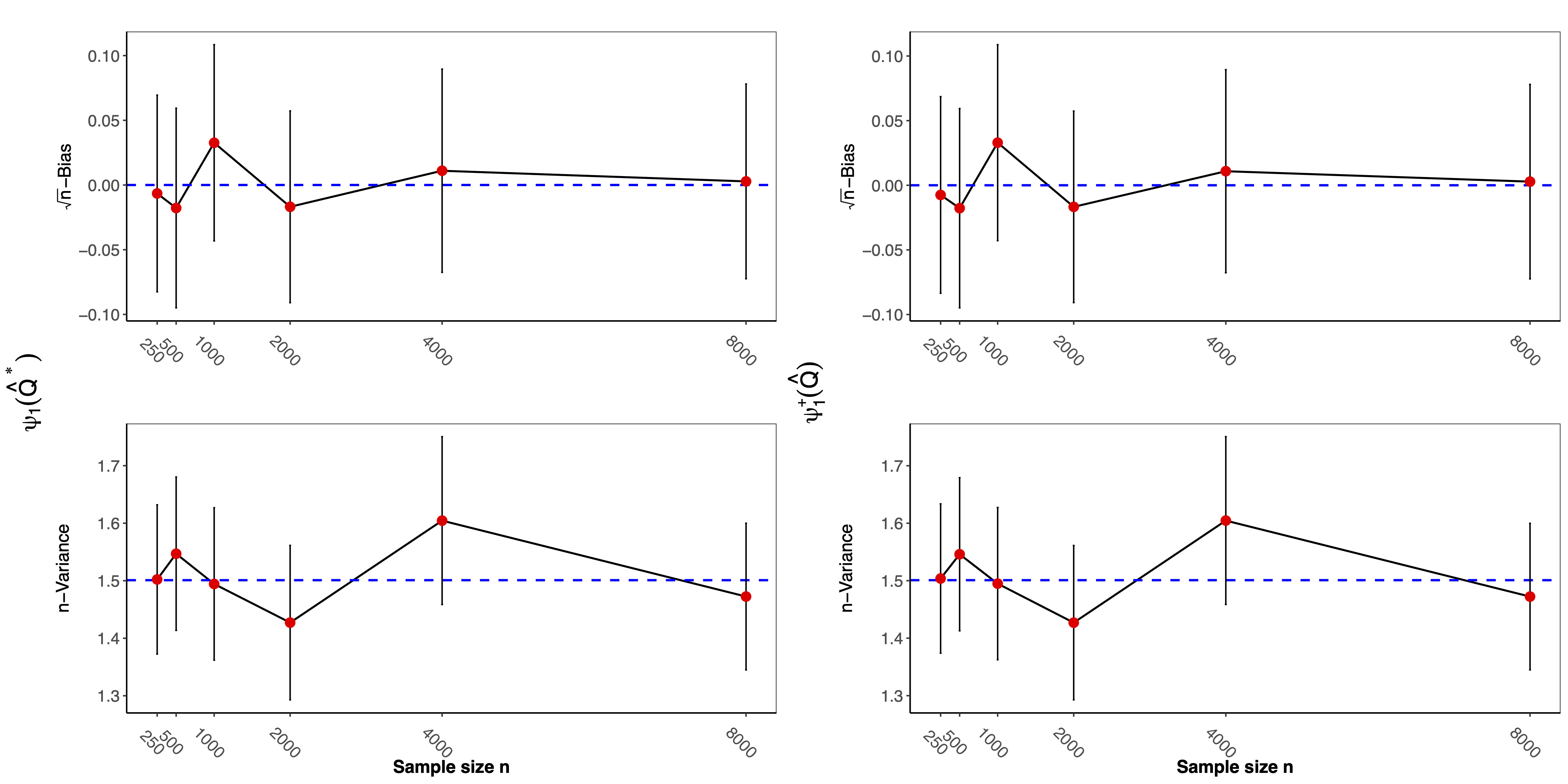
Figure 2: Simulation results validating the $n^{1/2}$-consistency behaviors, under univariate binary mediator. The left column is for TMLE and the right column is for the one-step estimator counterpart.

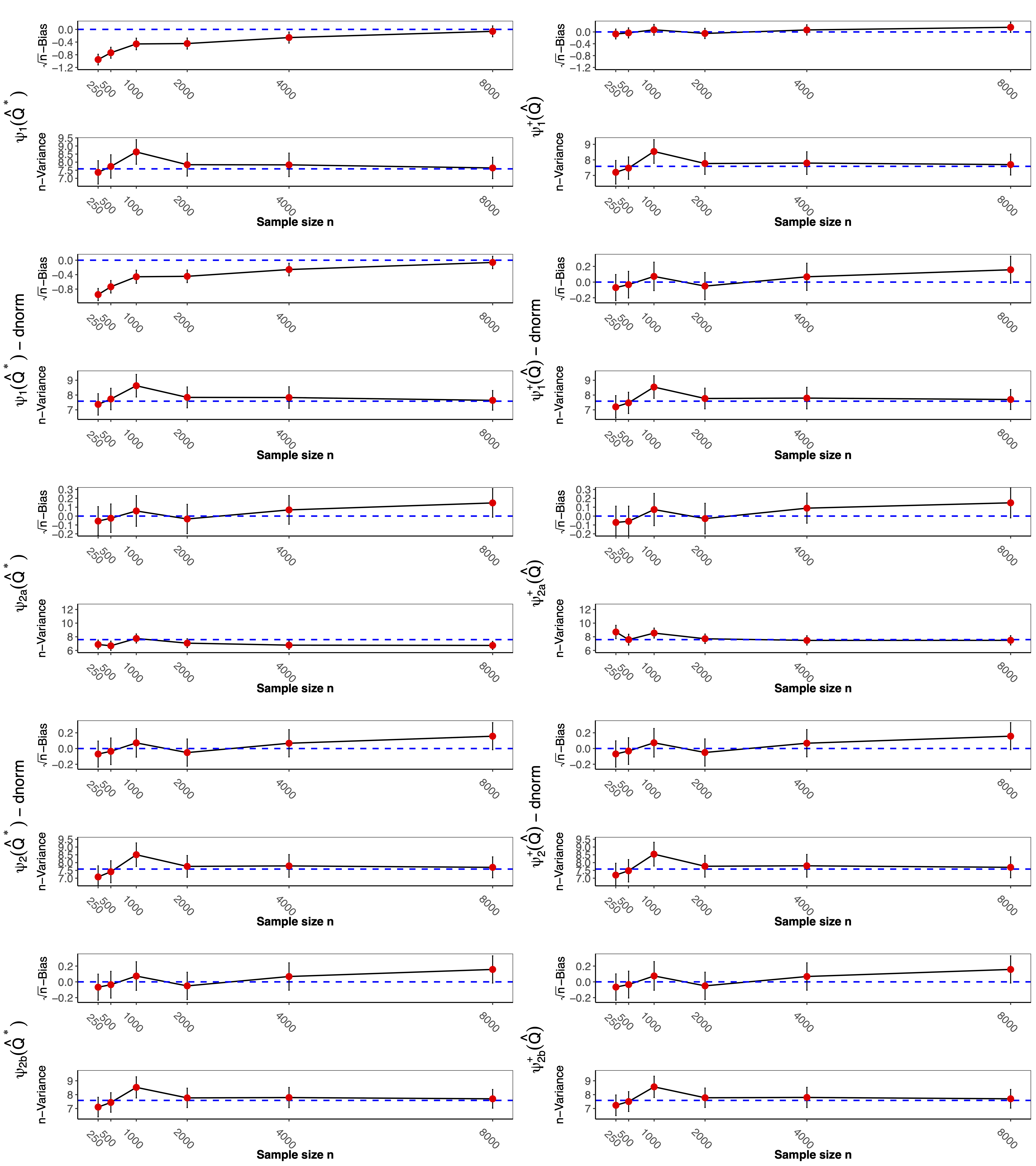
Figure 3: Simulation results validating the $n^{1/2}$-consistency behaviors, under univariate continuous mediator. The left column is for TMLE and the right column is for the one-step estimator counterpart.

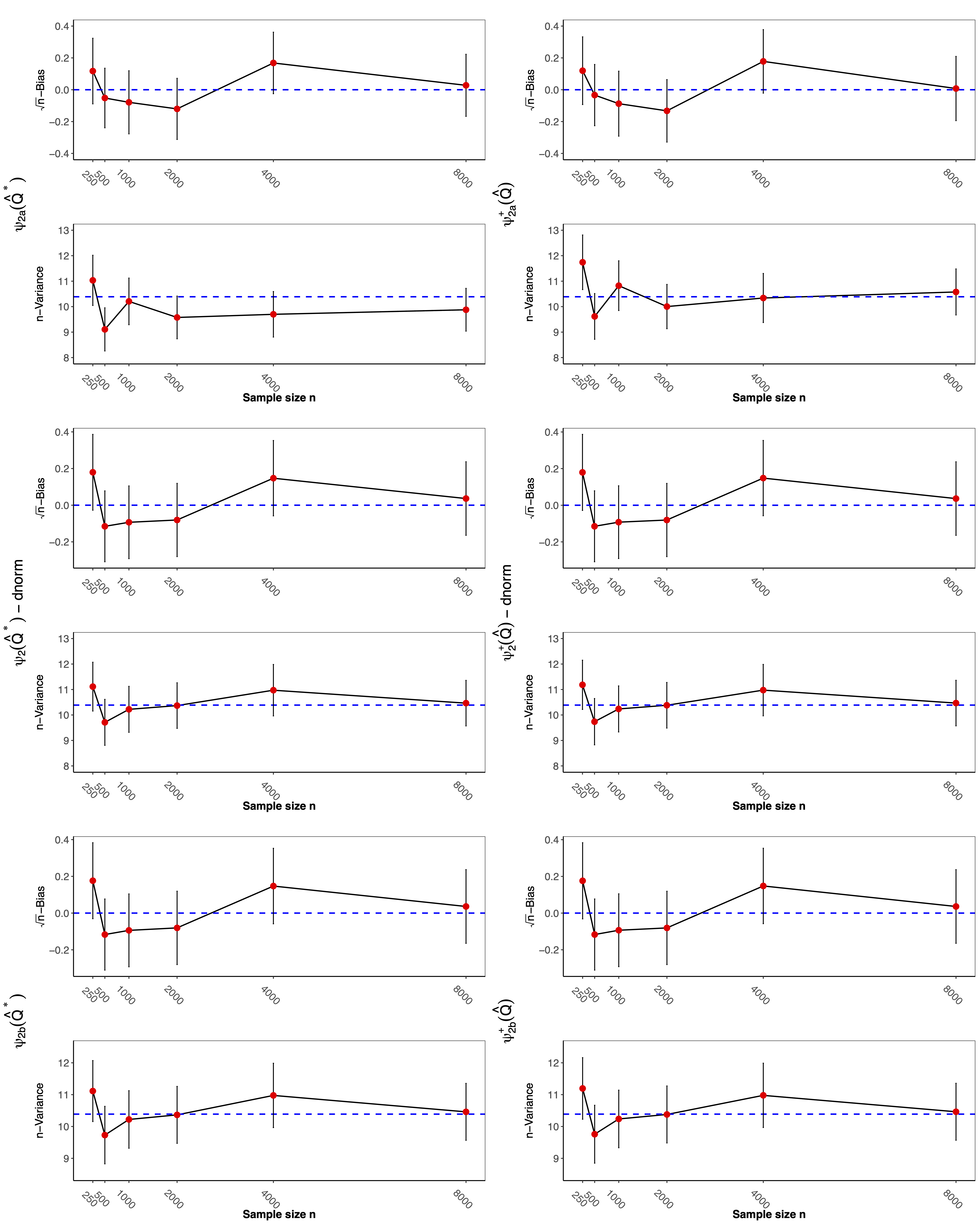
Figure 4: Simulation results validating the $n^{1/2}$-consistency behaviors, under bivariate continuous mediators. The left column is for TMLE and the right column is for the one-step estimator counterpart.

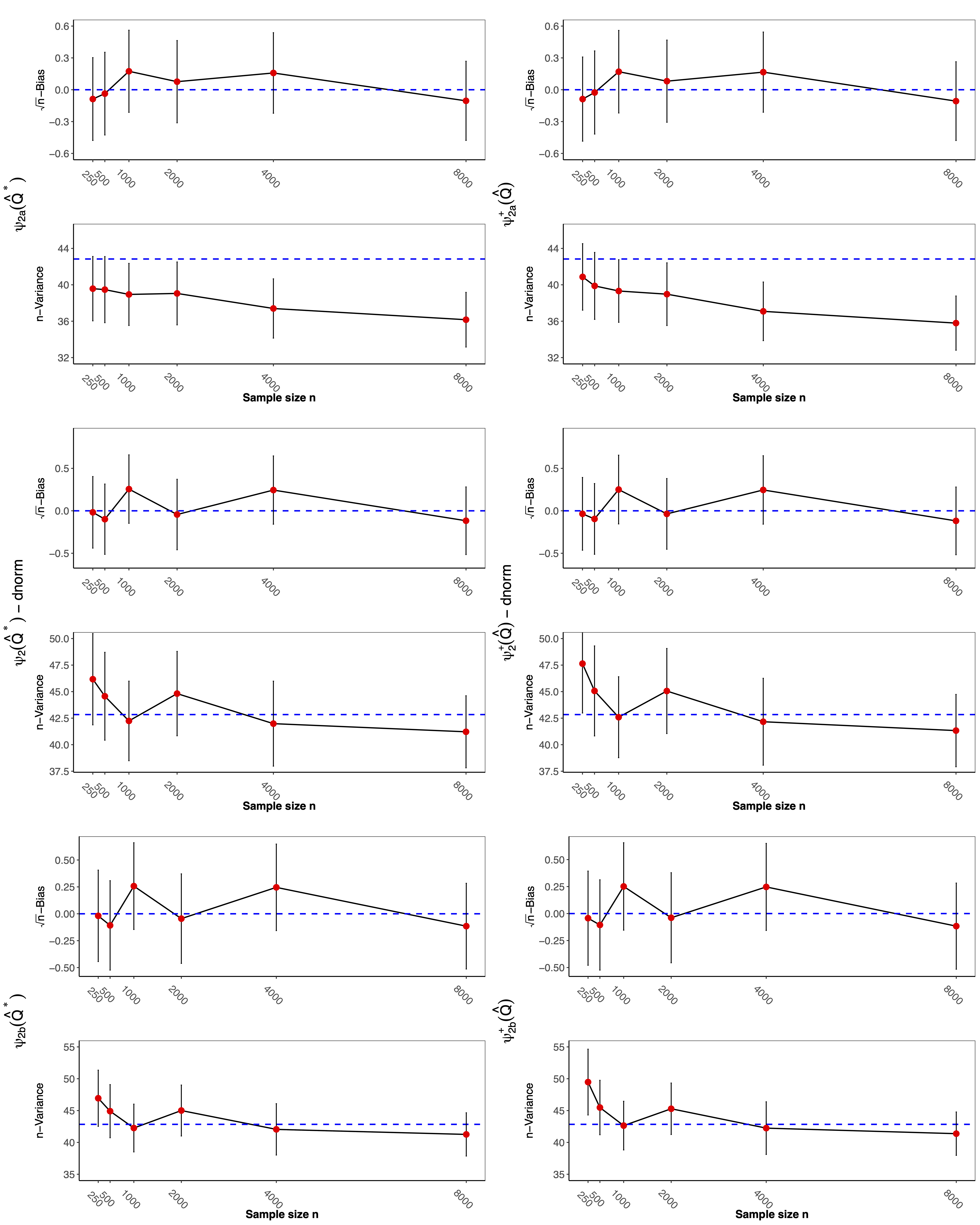
Figure 5: Simulation results validating the $n^{1/2}$-consistency behaviors, under quadrivariate continuous mediators. The left column is for TMLE and the right column is for the one-step estimator counterpart.

12.2 Simulation 2: TMLE vs. one-step in a setting with weak overlap

We generated the treatment variable according to $\operatorname{Binomial}\left(0.001+0.998X\right)$, while the rest of the DGPs, as specified in displays (41) and (42), remain unchanged.

12.3 Simulation 3: misspecified parametric models vs. flexible estimation

In our third set of simulations, we generated data according to the display in (43), where all variables are univariate.

$$X\sim\operatorname{Uniform}(0,1), \text{\small(binary) }M\sim\operatorname{Binomial}\big{(}\operatorname{expit}(-1+A+X-AX)\big{)},\vspace{0.1cm}$$ (43)

$$A\sim\operatorname{Binomial}\big{(}\operatorname{expit}(-1+X)\big{)}, \text{\small(continuous) }M\sim\mathcal{N}(1+A+X-AX,2),\vspace{0.1cm}$$

$$U\sim\mathcal{N}(1+A+X-AX,2), Y\sim\mathcal{N}(U+M+X-MX,2).\vspace{0.1cm}$$

12.4 Simulation 4: impact of cross-fitting

In our fourth set of simulations, we generated data according to the display in (44): “(binary)” indicates the DGP under binary mediator setup and “(continuous)” indicates the DGP under continuous mediator setup.

$$X_{i}\sim\operatorname{Uniform}(0,1),\ i\in\{1,\ldots,10\},$$ (44)

$$A\sim\mathrm{Binomial}(\mathrm{expit}(V_{A}\ [1\ X\ X^{2}]^{T})),$$

$$\text{\small(binary) }U\sim\mathcal{N}\left(V_{U}\ [1\ A\ X\ AX_{1-5}]^{T},2\right),$$

$$\text{\small(binary) }M\sim\mathrm{Binomial}\left(\mathrm{expit}\left(V_{M}\ [1\ A\ X\ AX_{1-5}\ X_{6-10}^{2}]^{T}\right)\right),$$

$$\text{\small(binary) }Y\sim\mathcal{N}\left(V_{Y}\ [U\ M\ X\ MX_{1-5}\ M^{2}\ X_{6-10}^{2}]^{T},2\right),$$

$$\text{\small(continuous) }U\sim\mathcal{N}\left(V_{U}\ [1\ A\ X\ AX_{1-5}]^{T},1\right),$$

$$\text{\small(continuous) }M\sim\mathcal{N}\left((V_{M}\ [1\ A\ X\ AX_{1-5}\ X_{6-10}^{2}]^{T}\right),1),$$

$$\text{\small(continuous) }Y\sim\mathcal{N}\left(V_{Y}\ [U\ M\ X\ MX_{1-5}\ M^{2}\ X_{6-10}^{2}]^{T},1\right).$$

where

$$V_{A}=0.1\times[0.48,0.07,1,-1,-0.34,-0.12,0.3,-0.35,1,-0.1,0.46,0.33,0,0.45,0.1,-0.32,-0.08,-0.2,0.5,0.5,-0.03]$$

$$V_{U}=[-2,-1,-1,2,3,0.5,3,2,-1,1,-3,1.5,-3,-2,1,3,1.5]$$

$$V_{M}=0.025\times[3,1.5,-1.5,-1.5,-1,-2,-3,-3,-1.5,2,1.5,3,1.5,2,0.5,0.5,3,-0.2,-0.33,0.5,0.3,-0.5]$$

$$V_{Y}=[1,-2,-3,-1.5,1,0.5,-2,1.5,-2,-3,-3,-1.5,-1,0.5,3,1.5,0.5,3,1,1.5,-2,3,-1]$$

$$X=[X_{1},X_{2},X_{3},X_{4},X_{5},X_{6},X_{7},X_{8},X_{9},X_{1}0]$$

$$X_{1-5}=[X_{1},X_{2},X_{3},X_{4},X_{5}]$$

$$X_{6-10}=[X_{6},X_{7},X_{8},X_{9},X_{10}]\ .$$

Table 6 reveals a comparative analysis using a more sensitive random forest algorithm by increasing the variability of predictions. Specifically, we adopted a sparser random forest with $200$ trees and a minimum node size of $1$. According to this table, the estimation performance of random forest is inferior, as evidenced by smaller CI coverage when compared with results produced by denser random forests (with $500$ trees). In contrast, results yielded by performing sample splitting in conjunction with the sparser random forest remains highly comparable to those shown in Tables 3. These findings imply that in high-dimensional settings or scenarios where high estimation variance is anticipated from nuisance estimates, cross-fitting proves beneficial in reducing estimation bias and enhancing the stability of results.

Table 6: Comparative analysis for the impact of cross-fitting on TMLEs and one-step estimators in conjunction with the use of random forests. RF refers to random forest with 200 trees and a minimum node size of 1, and CF denotes random forest with cross fitting using 5 folds.

	TMLEs						One-step estimators
	Univariate Binary		Univariate Continuous				Univariate Binary		Univariate Continuous
	$\psi_{1}(\hat{Q}^{\star})$		$\psi_{2a}(\hat{Q}^{\star})$		$\psi_{2b}(\hat{Q}^{\star})$		$\psi_{1}^{+}(\hat{Q})$		$\psi_{2a}^{+}(\hat{Q})$		$\psi_{2b}^{+}(\hat{Q})$
	RF	CF	RF	CF	RF	CF	RF	CF	RF	CF	RF	CF
n=500
Bias	-0.175	-0.021	-0.368	0.058	-0.518	0.020	-0.105	-0.027	-0.088	0.068	-0.524	0.018
SD	0.167	0.140	0.379	0.334	0.381	0.288	0.052	0.130	0.429	0.322	0.384	0.289
MSE	0.059	0.020	0.279	0.115	0.413	0.083	0.014	0.018	0.192	0.108	0.421	0.084
CI coverage	18.1%	83.9%	42.4%	87%	33.9%	88.4%	19.6%	86.6%	53.9%	88.2%	33%	87.7%
CI width	0.133	0.397	0.657	0.995	0.743	0.880	0.122	0.396	0.657	0.992	0.744	0.879
n=1000
Bias	-0.177	-0.016	-0.380	0.055	-0.520	0.013	-0.102	-0.020	-0.106	0.059	-0.525	0.010
SD	0.117	0.096	0.259	0.214	0.274	0.221	0.040	0.092	0.288	0.218	0.277	0.223
MSE	0.045	0.010	0.211	0.049	0.346	0.049	0.012	0.009	0.094	0.051	0.352	0.050
CI coverage	11.7%	89.5%	23.2%	89%	17.4%	87.6%	12.6%	90.6%	49.3%	87.9%	17.5%	88.2%
CI width	0.105	0.320	0.412	0.700	0.535	0.666	0.101	0.320	0.414	0.699	0.535	0.666
n=2000
Bias	-0.175	-0.010	-0.372	0.065	-0.498	0.025	-0.098	-0.012	-0.120	0.067	-0.504	0.021
SD	0.083	0.074	0.179	0.149	0.188	0.166	0.034	0.073	0.196	0.151	0.192	0.166
MSE	0.038	0.006	0.170	0.026	0.283	0.028	0.011	0.005	0.053	0.027	0.291	0.028
CI coverage	5.7%	90.9%	9.9%	89.7%	4.9%	85.9%	8.5%	91.1%	50.9%	89.4%	5.2%	86.3%
CI width	0.084	0.250	0.294	0.526	0.384	0.506	0.082	0.250	0.295	0.525	0.385	0.505

References

• Balke and Pearl [1994] A. Balke and J. Pearl. Counterfactual probabilities: Computational methods, bounds and applications. In Proceedings of UAI-94, pages 46–54, 1994.
• Bellemare et al. [2019] M. F. Bellemare, J. R. Bloem, and N. Wexler. The paper of how: Estimating treatment effects using the front-door criterion. Technical report, Working paper, 2019.
• Benkeser and Van Der Laan [2016] D. Benkeser and M. Van Der Laan. The highly adaptive lasso estimator. In 2016 IEEE international conference on data science and advanced analytics (DSAA), pages 689–696. IEEE, 2016.
• Bhattacharya and Nabi [2022] R. Bhattacharya and R. Nabi. On testability of the front-door model via verma constraints. In Uncertainty in Artificial Intelligence, pages 202–212. PMLR, 2022.
• Bhattacharya et al. [2022] R. Bhattacharya, R. Nabi, and I. Shpitser. Semiparametric inference for causal effects in graphical models with hidden variables. Journal of Machine Learning Research, 23:1–76, 2022.
• Bickel et al. [1993] P. J. Bickel, C. A. Klaassen, Y. Ritov, and J. A. Wellner. Efficient and adaptive estimation for semiparametric models, volume 4. Johns Hopkins University Press Baltimore, 1993.
• Chernozhukov et al. [2017] V. Chernozhukov, D. Chetverikov, M. Demirer, E. Duflo, C. Hansen, W. Newey, and J. Robins. Double/debiased machine learning for treatment and structural parameters. The Econometrics Journal, 2017.
• Fulcher et al. [2019] I. R. Fulcher, I. Shpitser, S. Marealle, and E. J. Tchetgen Tchetgen. Robust inference on population indirect causal effects: The generalized front-door criterion. Journal of the Royal Statistical Society, Series B, 2019.
• Glynn and Kashin [2013] A. Glynn and K. Kashin. Front-door versus back-door adjustment with unmeasured confounding: Bias formulas for front-door and hybrid adjustments. In 71st Annual Conference of the Midwest Political Science Association, volume 3, 2013.
• Glynn and Kashin [2018] A. N. Glynn and K. Kashin. Front-door versus back-door adjustment with unmeasured confounding: Bias formulas for front-door and hybrid adjustments with application to a job training program. Journal of the American Statistical Association, 113(523):1040–1049, 2018.
• Hahn [1998] J. Hahn. On the role of the propensity score in efficient semiparametric estimation of average treatment effects. Econometrica, pages 315–331, 1998.
• Hayfield and Racine [2008] T. Hayfield and J. S. Racine. Nonparametric econometrics: The np package. Journal of statistical software, 27:1–32, 2008.
• Hernán and Robins [2006] M. A. Hernán and J. M. Robins. Estimating causal effects from epidemiological data. Journal of Epidemiology & Community Health, 60(7):578–586, 2006.
• Hirano et al. [2003] K. Hirano, G. W. Imbens, and G. Ridder. Efficient estimation of average treatment effects using the estimated propensity score. Econometrica, 71(4):1161–1189, 2003.
• Huang and Valtorta [2006] Y. Huang and M. Valtorta. Pearl’s calculus of interventions is complete. In Twenty Second Conference On Uncertainty in Artificial Intelligence, 2006.
• Jorma [2018] K. Jorma. Life course 1971-2002 [dataset]. version 2.0, 2018. Finnish Social Science Data Archive [distributor]. http://urn.fi/urn:nbn:fi:fsd:T-FSD2076.
• Kanamori et al. [2009] T. Kanamori, S. Hido, and M. Sugiyama. A least-squares approach to direct importance estimation. The Journal of Machine Learning Research, 10:1391–1445, 2009.
• Kennedy [2022] E. H. Kennedy. Semiparametric doubly robust targeted double machine learning: a review. arXiv preprint arXiv:2203.06469, 2022.
• Manski [1990] C. F. Manski. Nonparametric bounds on treatment effects. The American Economic Review, 80(2):319–323, 1990.
• Neyman [1923] J. Neyman. Sur les applications de la thar des probabilities aux experiences agaricales: Essay des principle. excerpts reprinted (1990) in English. Statistical Science, 5:463–472, 1923.
• Pearl [1995a] J. Pearl. Causal diagrams for empirical research. Biometrika, 82(4):669–688, 1995a.
• Pearl [1995b] J. Pearl. Causal diagrams for empirical research. Biometrika, 82(4):669–709, 1995b. URL citeseer.ist.psu.edu/55450.html.
• Pearl [2009] J. Pearl. Causality: Models, Reasoning, and Inference. Cambridge University Press, 2 edition, 2009. ISBN 978-0521895606.
• Richardson and Robins [2013] T. S. Richardson and J. M. Robins. Single world intervention graphs (SWIGs): A unification of the counterfactual and graphical approaches to causality. 2013.
• Richardson et al. [2017] T. S. Richardson, R. J. Evans, J. M. Robins, and I. Shpitser. Nested markov properties for acyclic directed mixed graphs. arXiv preprint arXiv:1701.06686, 2017.
• Robins [1986] J. M. Robins. A new approach to causal inference in mortality studies with sustained exposure periods – application to control of the healthy worker survivor effect. Mathematical Modeling, 7:1393–1512, 1986.
• Robins et al. [1994a] J. M. Robins, A. Rotnitzky, and L. P. Zhao. Estimation of regression coefficients when some regressors are not always observed. Journal of the American Statistical Association, 89(427):846–866, 1994a.
• Robins et al. [1994b] J. M. Robins, A. Rotnitzky, and L. P. Zhao. Estimation of regression coefficients when some regressors are not always observed. Journal of the American Statistical Association, 89:846–866, 1994b.
• Robins et al. [2000] J. M. Robins, A. Rotnitzky, and D. O. Scharfstein. Sensitivity analysis for selection bias and unmeasured confounding in missing data and causal inference models. In Statistical models in epidemiology, the environment, and clinical trials, pages 1–94. Springer, 2000.
• Rosenbaum and Rubin [1983] P. R. Rosenbaum and D. B. Rubin. The central role of the propensity score in observational studies for causal effects. Biometrika, 70:41–55, 1983.
• Rubin [1974] D. B. Rubin. Estimating causal effects of treatments in randomized and non-randomized studies. Journal of Educational Psychology, 66:688–701, 1974.
• Scharfstein et al. [2021] D. O. Scharfstein, R. Nabi, E. H. Kennedy, M.-Y. Huang, M. Bonvini, and M. Smid. Semiparametric sensitivity analysis: Unmeasured confounding in observational studies. arXiv preprint arXiv:2104.08300, 2021.
• Shpitser and Pearl [2006] I. Shpitser and J. Pearl. Identification of joint interventional distributions in recursive semi-Markovian causal models. In Proceedings of the Twenty-First National Conference on Artificial Intelligence (AAAI-06). AAAI Press, Palo Alto, 2006.
• Sugiyama et al. [2007] M. Sugiyama, S. Nakajima, H. Kashima, P. Buenau, and M. Kawanabe. Direct importance estimation with model selection and its application to covariate shift adaptation. Advances in neural information processing systems, 20, 2007.
• Sugiyama et al. [2010] M. Sugiyama, M. Kawanabe, and P. L. Chui. Dimensionality reduction for density ratio estimation in high-dimensional spaces. Neural Networks, 23(1):44–59, 2010.
• Tian and Pearl [2002] J. Tian and J. Pearl. A general identification condition for causal effects. In Eighteenth National Conference on Artificial Intelligence, pages 567–573, 2002. ISBN 0-262-51129-0.
• Tsiatis [2007] A. Tsiatis. Semiparametric theory and missing data. Springer Science & Business Media, 2007.
• van der Laan and Rubin [2006] M. J. van der Laan and D. Rubin. Targeted maximum likelihood learning. The International Journal of Biostatistics, 2(1), 2006.
• Van der Laan et al. [2007] M. J. Van der Laan, E. C. Polley, and A. E. Hubbard. Super learner. Statistical applications in genetics and molecular biology, 6(1), 2007.
• van der Laan et al. [2011] M. J. van der Laan, S. Rose, et al. Targeted learning: causal inference for observational and experimental data, volume 4. Springer, 2011.
• van der Vaart and Wellner [2023] A. van der Vaart and J. A. Wellner. Empirical processes. In Weak Convergence and Empirical Processes: With Applications to Statistics, pages 127–384. Springer, 2023.
• van der Vaart [2000] A. W. van der Vaart. Asymptotic Statistics, volume 3. Cambridge University Press, 2000.
• Verma and Pearl [1990] T. S. Verma and J. Pearl. Equivalence and synthesis of causal models. Technical Report R-150, Department of Computer Science, University of California, Los Angeles, 1990.
• Wen et al. [2023] L. Wen, A. L. Sarvet, and M. J. Stensrud. Causal effects of intervening variables in settings with unmeasured confounding. arXiv preprint arXiv:2305.00349, 2023.
• Yamada et al. [2013] M. Yamada, T. Suzuki, T. Kanamori, H. Hachiya, and M. Sugiyama. Relative density-ratio estimation for robust distribution comparison. Neural computation, 25(5):1324–1370, 2013.
• Zheng and Van Der Laan [2010] W. Zheng and M. J. Van Der Laan. Asymptotic theory for cross-validated targeted maximum likelihood estimation. 2010.
{appendices}