Large Scale Structure in COSMOS2020: Evolution of Star Formation Activity in Different Environments at $0.4<z<4$

Abstract

To study the role of environment in galaxy evolution, we reconstruct the underlying density field of galaxies in COSMOS2020 (The Farmer catalog) and provide the density catalog for a magnitude limited ($K_{s}<24.5$) sample of $\sim 210\,k$ galaxies at $0.4<z<5$ within the COSMOS field. The environmental densities are calculated using weighted Kernel Density Estimation (wKDE) approach with the choice of von Mises-Fisher kernel, an analog of the Gaussian kernel for periodic data. Additionally, we make corrections for the edge effect and masked regions in the field. We utilize physical properties extracted by LePhare to investigate the connection between star formation activity and the environmental density of galaxies in six mass-complete sub-samples at different cosmic epochs within $0.4<z<4$. Our findings confirm a strong anti-correlation between star formation rate (SFR)/specific SFR (sSFR) and environmental density out to $z\sim 1.1$. At intermediate redshifts $1.1<z<2$, there is no significant correlation between SFR/sSFR and density. At higher redshifts $2<z<4$ we observe a reversal of the SFR/sSFR-density relation such that the SFR increases by a factor of $\sim 10$ with increasing density contrast, $\delta$, from -0.4 to 5. This observed trend might be due to the greater availability of gas-content in high-density environments, potentially leading to increased star formation rates in galaxies residing in rich environments at $z>2$.

1 Introduction

Galaxies in the universe are distributed in a web-like structure known as “Cosmic Web” (Bond et al., 1996). The study of these large-scale structures (hereafter LSS), which comprise galaxy clusters, sparsely populated voids, filamentary threads, and planar walls, is a cornerstone in our understanding of the evolution of galaxies and dark matter, which are strongly connected.

The identification of LSS and the study of matter distribution within the cosmic web is still challenging due to the diverse shape and size of LSS, which often confines such studies to local-universe spectroscopic surveys (York et al., 2000; Colless et al., 2001), simulations (Cautun et al., 2014; Vogelsberger et al., 2014; Libeskind et al., 2018), and analytical methods (Bardeen et al., 1986; Bond et al., 1996; Sousbie, 2011; AnsariFard et al., 2022). However, with the advent of wide and deep photometric surveys using ground and space telescopes, such as The Cosmic Evolution Survey (COSMOS), we are now able to identify and study these structures and their impact on the galaxy evolution in the high-redshift universe. Several studies have confirmed and investigated LSS in the COSMOS field, including the following examples: study of a large filamentary structure, known as COSMOS wall, at $z\sim 0.73$ (Iovino et al., 2016), spectroscopic confirmation/investigation of a large scale structure at $z\sim 2.1$ (Hung et al., 2016), a proto-cluster at $z\sim 2.23$ (Darvish et al., 2020), an asymmetric filamentary structure at $z\sim 2.47$ (Casey et al., 2015), a concentrated group of massive galaxies with extended X-ray emission at $z\sim 2.506$ (Wang et al., 2016), massive proto-clusters at $z\sim 3.3$ (Forrest et al., 2023), $z\sim 3.366$ (McConachie et al., 2022), $z\sim 4.57$ (Lemaux et al., 2018), and $z\sim 5.3$ (Capak et al., 2011), discovery of a massive, dusty starburst galaxy in a protocluster at $z\sim 5.7$ (Pavesi et al., 2018) and complex-shaped overdensities in photometric redshifts at $z\sim 2.45$ (Cucciati et al., 2018). Additionally, overdensities in 3D Ly$\alpha$ forest tomography are studied as alternative tracers of LSS (e.g., CLAMATO, Lee et al. 2016 and LATIS, Newman et al. 2020 surveys).

In addition to the identification of LSS in the spectroscopic and photometric surveys, the study of galaxy properties, such as morphology (Mandelbaum et al., 2006; Capak et al., 2007; Bamford et al., 2009), gas content (Catinella et al., 2013), star formation activity (Scoville et al., 2013; Darvish et al., 2016; Chartab et al., 2020), and quenching mechanisms (Peng et al., 2010) in different environments have become increasingly important in the past few years.

Studies show that in the local universe, early-type passive galaxies are typically found in denser environments, such as galaxy clusters, while late-type star-forming galaxies are mainly located in less-dense regions, known as field (Dressler, 1980; Balogh et al., 2004; Kauffmann et al., 2004; Peng et al., 2010; Woo et al., 2012; Baldry et al., 2006). This is partly because in addition to internal processes (mass-quenching), galaxies in denser environments have experienced an enhanced level of “environmental quenching” such as ram pressure stripping (Gunn & Gott, 1972), galaxy harassment (Moore et al., 1996), and galaxy-galaxy interactions (Farouki & Shapiro, 1981).

At intermediate redshifts (out to $z\sim 1.4$), (Capak et al., 2007) investigated the density-morphology relations, finding that galaxies are transformed from late (spiral and irregular) to early-type galaxies more rapidly in dense regions compared to sparse regions.

While these trends are well-established in the low-redshift universe, they remain a matter of ongoing debate at intermediate and higher redshifts ($z\gtrsim 1$). (Patel et al., 2009) reports a negative correlation between star formation activity and environmental density at $z\sim 0.83$, the same as the local universe. Some studies find no significant correlation between SFR and environment beyond redshift $z\sim 1$ (Grützbauch et al., 2011; Scoville et al., 2013; Darvish et al., 2016; Chartab et al., 2020). In contrast, a positive correlation between SFR/sSFR and environmental density is reported in (Elbaz, D. et al., 2007; Cooper et al., 2008) and (Lemaux et al., 2022) reports a reversal of the SFR-density relation at $2<z<5$. This discrepancy between high redshift results is due to the limited availability of observational data at higher redshifts, a lack of complete samples of statistically significant size, and more uncertainties in the extracted physical parameters for fainter objects. This weakens the statistical reliability of these trends at higher redshifts, making the interpretation of these observations more challenging. Thus, more studies are needed to reliably identify the LSS at higher redshifts and investigate the role of the environment in the star formation activity of galaxies in the early stages of galaxy evolution.

COSMOS data spans a large area of ($\sim 2\,\text{deg}^{2}$) which enables us to investigate these correlations in a variety of environments with potentially lower impacts of cosmic variance on the results. It is important to note that COSMOS does not appear to have many massive structures at ($z\lesssim 2$), and the dynamic range of overdensities at low redshifts is fairly small when compared to the other local-universe surveys (SDSS, York et al. 2000) or those that specifically target fields that contain massive LSS at $z\sim 1$ (e.g., EdisCS, White et al. 2005; GOGREEN, Balogh et al. 2017; ORELSE, Lubin et al. 2009). Nonetheless, COSMOS2020, with its deeper optical, infrared, and near-infrared data compared to previous releases, still offers an opportunity to extend studies of LSS and environmental effects to higher redshifts.

To start our analysis, we first need to clarify what we mean by “environmental density”. Numerous methods have been used in the literature to estimate the density field associated with a given distribution of galaxies. A comprehensive review and comparison between these methods including “weighted Kernel Density Estimation” (wKDE), “weighted K-Nearest Neighbor”, “weighted Voronoi Tesselation”, and “weighted Delaunay Triangulation” is provided by (Darvish et al., 2015). Examining the performance of all these methods on simulated data, (Darvish et al., 2015) conclude that the weighted Kernel Density (wKDE) and Voronoi tesselation best reproduce the underlying density field in simulated data.

In this study, we adopt wKDE method with the choice of von Mises-Fisher kernel function to estimate the underlying density field at different redshifts using COSMOS2022. We produce density maps out to $z\sim 5$ which can be used to identify LSS and release a publicly available catalog of measured densities for 210621 galaxies brighter than $K_{s}<24.5$ at $0.4<z<5$ in the COSMOS field. We implement corrections to mitigate edge effects and masked sources in the vicinity of bright stars to improve the quality of density estimation. Eventually, we investigate the relationship between estimated environmental density and the star formation activity (SFR/sSFR) at different redshift intervals to study the evolution of this relationship with cosmic time.

The paper is organized as follows: In Section 2, we introduce the properties of data and selection criteria we used in this study. In Section 3, we describe the method used to construct density maps and the environmental density catalog, followed by the results and discussion in Section 4. We summarize our findings in Section 5.

Throughout this work, we assume a flat $\Lambda\text{CDM}$ cosmology with $H_{0}=70\,\text{km}\,s^{-1}\text{Mpc}^{-1}$ , $\Omega_{m0}=0.3$, and $\Omega_{\Lambda 0}=0.7$. All magnitudes are expressed in the AB system and the physical parameters are measured assuming a Chabrier initial mass function.

2 Data

COSMOS2020 consists of $\sim 1.7$ million sources for which source detection and multiwavelength photometry (X-ray to radio-imaging) are performed across the $\sim 2\,\text{deg}^{2}$ of the equatorial COSMOS field (Weaver et al., 2022). In addition to the previous release of this catalog (COSMOS2015, Laigle et al. 2016), COSMOS2020 consists of new ultra-deep optical data from the Hyper Supreme-Cam (HSC) Subaru Strategic Program (SSP), new visible Infrared Survey Telescope for Astronomy (VISTA) data from DR4 reaching more than one magnitude deeper in the $K_{s}$ band over the full area. Deep $u^{\star}$- and new u-band imaging from the Canada-France-Hawaii Telescope program CLAUDS (Sawicki et al., 2019) provides us with a deep coverage over a greater area than COSMOS2015.

Among these sources, around $966000$ are measured with all available broadband data utilizing two photometry tools 1) traditional aperture photometry (Laigle et al., 2016), the “CLASSIC” catalog, and 2) a new profile-fitting photometric tool, “The Farmer” (Weaver et al., 2023), each of which includes photometric redshifts (hereafter photo-$z$) and other physical parameters computed by EASY (Brammer et al., 2008) and LePhare (Ilbert et al., 2006; Arnouts et al., 2002). photo-$z$s calculated in both The Farmer and CLASSIC catalogs are corrected for dust extinction using the (Schlafly & Finkbeiner, 2011) dust map. In this study, we use the combination of The Farmer catalog with physical parameters extracted by LePhare.

The Farmer is a profile-fitting photometry package that combines a library of smooth parametric models from The Tractor (Lang et al., 2016) with a decision tree that aims to determine the best-fit model in harmony with neighboring (blended) sources. The resulting photometric measurements are naturally total, without the need for aperture corrections, and more reliable in deep extragalactic fields with more crowded regions (Weaver et al., 2022). According to (Weaver et al., 2023), The Farmer is particularly effective at deblending sources in low-resolution images like IRAC. In contrast, aperture photometry (the CLASSIC catalog) may underestimate the total flux of the sources and does not simultaneously model blended objects. Overall, the photo-$z$ quality is similar between the two catalogs but, as noted by (Weaver et al., 2022), The Farmer demonstrates superior performance at fainter magnitudes which predominantly correspond to high-redshift sources. This aspect particularly led us to choose The Farmer catalog for this study. The photometry quality of both catalogs is compared in detail in (Weaver et al., 2022).

For the physical parameters, we use the results extracted by LePhare (Arnouts et al., 2002; Ilbert et al., 2006) which uses the same configuration outlined in (Ilbert et al., 2013) to fit both galaxy and stellar templates to the observed photometry. As the first step, photo-$z$s are estimated following the method outlines in (Laigle et al., 2016), then the physical properties such as absolute magnitudes, star formation rates (SFR/sSFR), and stellar mass are computed with the same configuration as COSMOS2015: LePhare fits a template library generated by (Bruzual & Charlot, 2003) models to the observed photometry after fixing the redshift of each target to the estimated photo-$z$ in the first step. Further details are discussed in (Laigle et al., 2016; Weaver et al., 2022).

The catalog contains photometric measurements in 44 bands (including $U$-band, Optical, Near-infrared, Mid-infrared, X-ray, UV, and HST data), area flags, object type, and physical parameters such as SFR, sSFR, and stellar mass. We limit our study to a sub-sample of 211431 galaxies with the following selection criteria:

• Photo-$z$ range of $0.4<z<6$: while we report environmental densities for sources out to $z\sim 5$ and the primary focus of our star formation activity-environment analysis is on sources within $0.4<z<4$, we considered a buffer range ($4<z<6$) at the high redshift end of our primary redshift range to capture the full redshift Probability Distribution Function (zPDF) of sources whose zPDFs extend tails beyond $z=4$. Since zPDFs are narrower for low-redshift sources, there is no need for a buffer range at the lower end of our redshift range. Because of the sparsity of sources and a bias toward brighter sources, the reliability of the reconstructed density fields significantly diminishes beyond $z=4$.

• We filter out sources with large uncertainties in their photo-$z$ measurements ($\Delta z>2$). $\Delta z$ is the 68% confidence interval on estimated photo-$z$. These sources do not effectively contribute to the density field. The relative median redshift uncertainty of the filtered sample is $\Delta z/(1+z)\lesssim 0.02$ throughout the entire redshift range.

• An area of $\sim 1.7\,deg^{2}$ enclosed within $1.604<\delta<2.817$ and $149.398<\alpha<150.787$. This is the largest region containing robust NIR imaging equating to a spatially homogeneous selection function and NIR coverage.

• LePhare separates galaxies from stars and AGNs by combining morphological and SED criteria. We use a pure sample of “galaxies” (as identified by LePhare) that are not in the “bright star” masks.

• A magnitude cut of $K_{s}\sim 24.5$ to remove faint sources with unreliable physical parameters extracted from SED fitting. Fainter sources do not contribute effectively to the reconstructed density field due to large uncertainties in their photo-$z$.

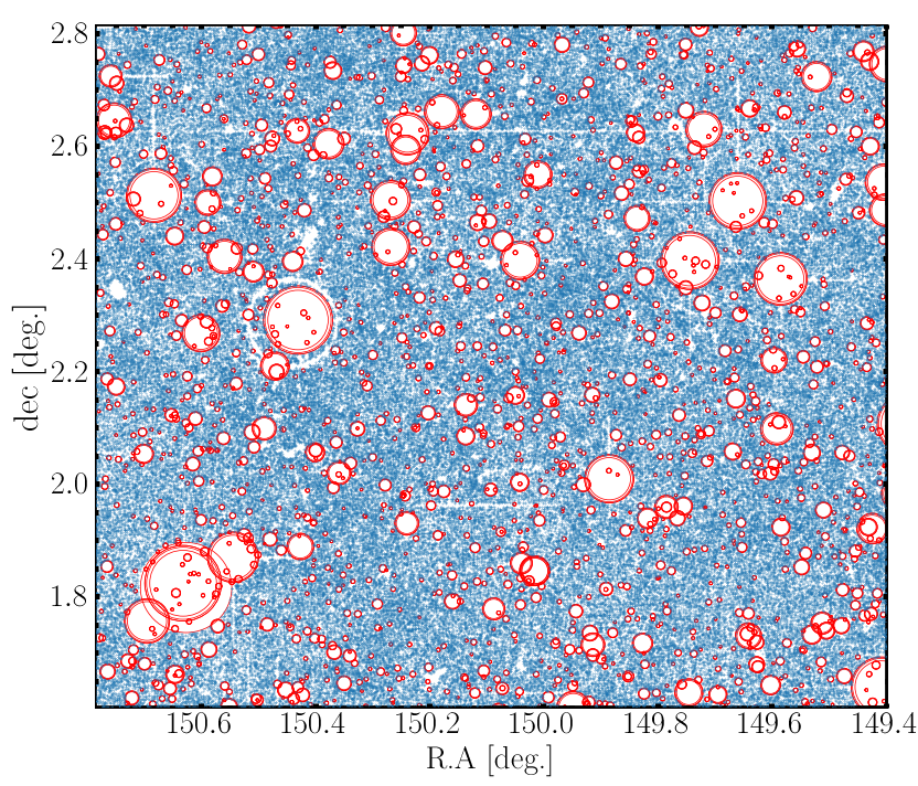
Figure 1: Spatial distribution of sources selected based on criteria outlined in Section 2. Red circles show bright star masks from the HSC-SSP PDR2 ($\sim 7600$ regions) provided by (Coupon et al., 2017) which are used to mask objects in the vicinity of bright stars.

Figure 1 shows the spatial distribution of the resulting sample across the field. The red circles in figure 1 show masked regions that contain sources in the vicinity of bright stars (Coupon et al., 2017). There are $\sim 7600$ such masked regions in the area of our interest.

3 Density Field Estimation

We calculate the environmental densities adopting the same approach introduced in Chartab et al. (2020) with minor modifications detailed in the following sections. Although we refer the reader to Chartab et al. (2020) for more comprehensive details, we summarize the key steps of the method in this following section for clarity, and to contextualize the modifications we implemented.

3.1 Weighted Kernel Density Estimation

wKDE is a non-parametric method used for density reconstruction based on the spatial distribution of data points (Parzen, 1962; A. Guillamón & Ruiz, 1998; Gisbert, 2003; Darvish et al., 2015), and is especially effective in handling weighted data. To reconstruct the density field utilizing wKDE, we implement the following procedure: 1) dividing the sample into redshift slices (Section 3.2), 2) calculating weights for all galaxies in each redshift slice (Section 3.3), 3) applying corrections to improve the density estimation around the masked regions (Section 3.4), 4) find the optimum bandwidth in each redshift slice and an adaptive bandwidth for each source (Section 3.5), 5) applying corrections for the “edge effect” that impacts calculated densities near the edges of the field (Section 3.6).

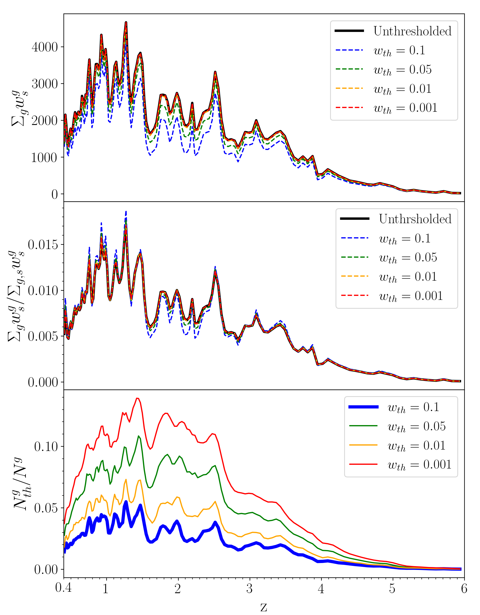
Figure 2: Top: the effective number of galaxies ($\sum_{g}w_{s}^{g}$) in each slice, for different thresholds on weight: 0.1, 0.05, 0.01, 0.001. The black curve shows the full sample without a threshold on weights. Middle: the effective number of galaxies in each redshift slice divided by the effective number of galaxies in all slices. Bottom: the size of the thresholded sample divided by the size of the unthresholded sample in each redshift slice. This fraction shows the degree to which thresholding lessens the computational time in the density estimate stage.

In this scheme, the surface density for the $i$th galaxy in the $s$th redshift slice and at position ($X_{i}$) is defined as:

$$\sigma^{s}(X_{i})=\sum_{g}w_{g}^{s}K(X_{i};X_{g})$$ (1)

where, $K(X_{i};X_{g})$, is the Kernel function of our choice calculated between two sources at $X_{i}$ and $X_{g}$ and $w_{g}^{s}$ is the probability of galaxy $g$ being at $s$th redshift slice normalized to the sum of its weights in all redshift slices. In this work, we adopt the “von Mises-Fisher” kernel function, which is the analog of the Gaussian kernel function for circular/periodic data (here R.A and Dec. coordinates) (Bai et al., 1988; García-Portugués et al., 2013; Taylor, 2008; Chartab et al., 2020). The “von Mises-Fisher” kernel is a simplified, isotropic form of a more general 5-parameter kernel function known as “Kent” distribution (Kent, 1982). While the “von Mises-Fisher” kernel effectively reduces to the Gaussian kernel in small fields, its use is particularly advantageous for providing greater accuracy in future wide-field surveys:

$$K(X_{i};X_{g})=\frac{1}{4\pi b^{2}\sinh(1/b^{2})}\exp\left(\frac{\cos\psi}{b^{2}}\right)$$ (2)

Where $\psi$ is the angular distance between $X_{i}$ and $X_{g}$ which can be calculated using their coordinates and $b$ is the bandwidth of this kernel which determines the extent to which the source at position $X_{g}$ contributes to the environmental density of the source at position $X_{i}$. Details of finding the optimum value of $b$ are explained in Section 3.5.

Eventually, We calculate the environmental density for the $i$th galaxy in our sample, $\sigma(G_{i})$, as a weighted sum of the surface density across all redshift slices (Chartab et al., 2020):

$$\sigma(G_{i})=\sum_{s}w_{i}^{s}\sigma^{s}(X_{i})$$ (3)

Where $w_{i}^{s}$ is the weight associated with the galaxy $i$ at $s$th slice.

3.2 Redshift Slices

To reconstruct the density field at different redshifts we have two options to deal with the uncertainties of photo-$z$s. One is to adopt wide enough, overlapping redshift slices to consider the contribution of galaxies that have large uncertainties on their photo-$z$ and those that are close to the boundaries of each slice. In this approach, the width of slices is chosen based on the redshift uncertainties. For instance, the median of the photo-$z$ uncertainties can be considered as the width of the redshift slices (Darvish et al., 2015; Scoville et al., 2013).

An alternative approach, which we used in this work, is to assign a weight to each galaxy at all redshift slices to incorporate their contribution at all redshift slices according to their photo-$z$ PDF (Chartab et al., 2020). In this approach, we no longer need to have overlapping slices. We divide our redshift range into slices with a constant comoving width. For that, we need to define a physically reasonable length scale as the width of redshift slices. This comoving length should be larger than the typical size of structures of our interest (e.g. galaxy clusters), account for the uncertainties in photo-$z$ measurements, and the uncertainty in the redshift direction caused by the peculiar velocity of galaxies in the line of sight, known as redshift space distortion (RSD). Due to RSD, an internal velocity dispersion of $\Delta v$ for a galaxy cluster at redshift z can be translated to a comoving distortion of value $\Delta\chi$ in the line of sight:

$$\Delta\chi=\frac{\Delta v}{H_{0}}\frac{1+z}{\sqrt{\Omega_{m0}(1+z)^{3}+\Omega_{\Lambda 0}}}$$ (4)

This length scale, due to the RSD limitation, peaks at $z=(2\Omega_{\Lambda 0}/\Omega_{m0})^{1/3}-1\approx 0.65$: A massive galaxy cluster with internal velocity dispersion $\Delta v\approx 1500\,km\,s^{-1}$ will be extended $\approx 18\,h^{-1}\,\text{Mpc}$ in comoving space.

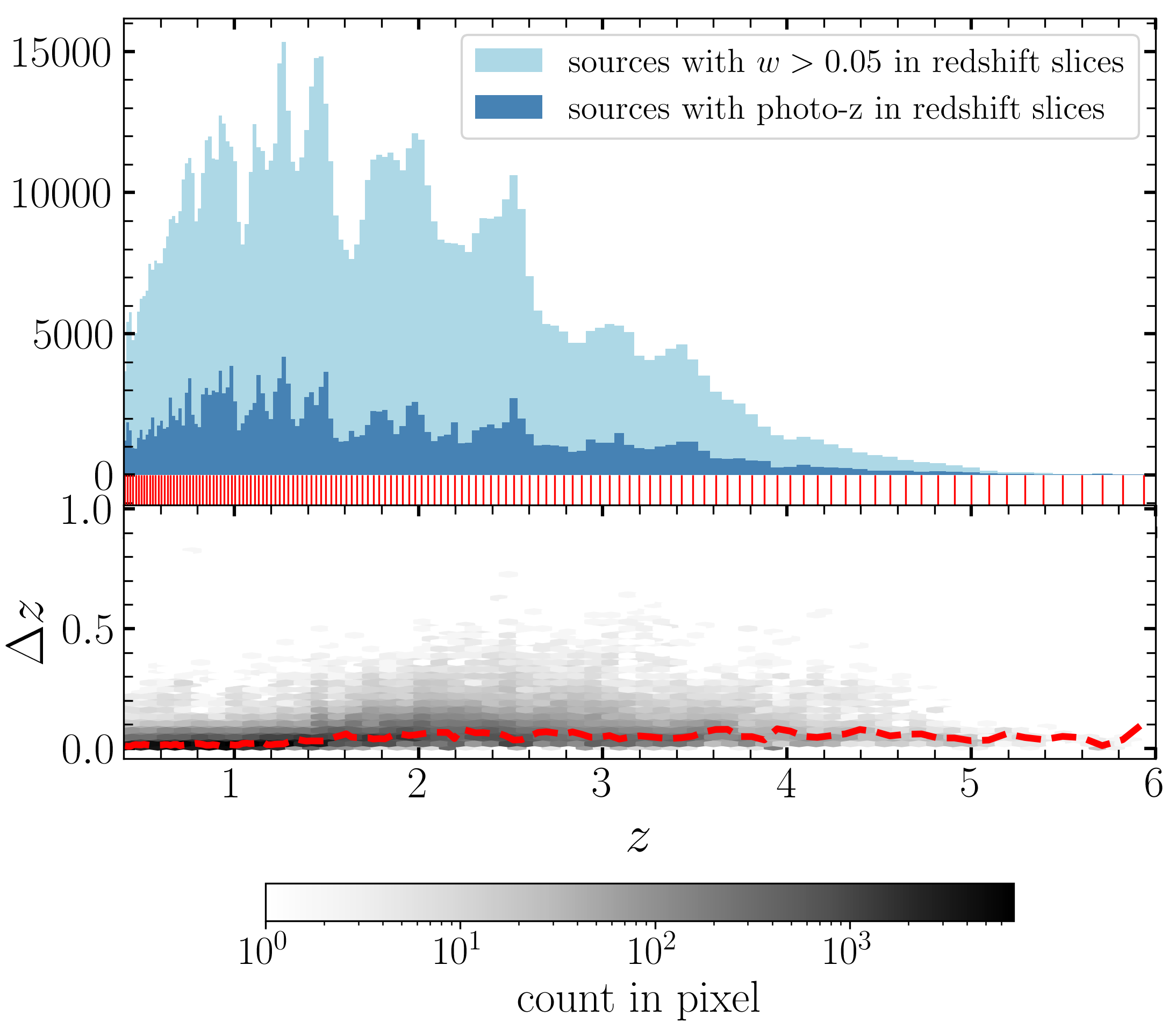
Figure 3: Top: shows the distribution of galaxies within $0.4<z<6$. The dark blue histogram represents the count of galaxies that have photo-$z$ measurement within a redshift slice and the light blue histogram shows the distribution of galaxies that have weights above $w_{th}=0.05$ in each redshift slice. Redshift slice centers are shown as vertical red lines between two panels. Bottom: shows the photo-$z$ uncertainty (half of the $68\%$ confidence interval of photo-$z$) as a function of redshift. The dashed red line shows the median of the photo-$z$ uncertainties in each redshift slice.

Another constraint in redshift binning is the uncertainty of photo-$z$ measurements. A choice of $\Delta\chi=35\,h^{-1}\text{Mpc}$ leads us to a relative median uncertainty $\Delta z/(1+z)<0.02$ in all redshift slices, while it satisfies the minimum required width needed to account for the RSD effect and it is bigger than the typical size of LSS up to $z_{max}\sim 6$.

One can translate this comoving width, $\Delta\chi$, into width of the redshift slices $\Delta z$:

$$\Delta z=\frac{\Delta\chi H_{0}}{c}\left[\Omega_{m}(1+z)^{3}+\Omega_{\Lambda}\right]^{0.5}$$ (5)

The choice of $\Delta\chi=35\,h^{-1}\text{Mpc}$ leads us to 135 redshift slices ranging from $z=0.4$ to $z=6$, with slice widths varying from 0.014 (at redshift 0.4) to 0.117 (at redshift 5.936).

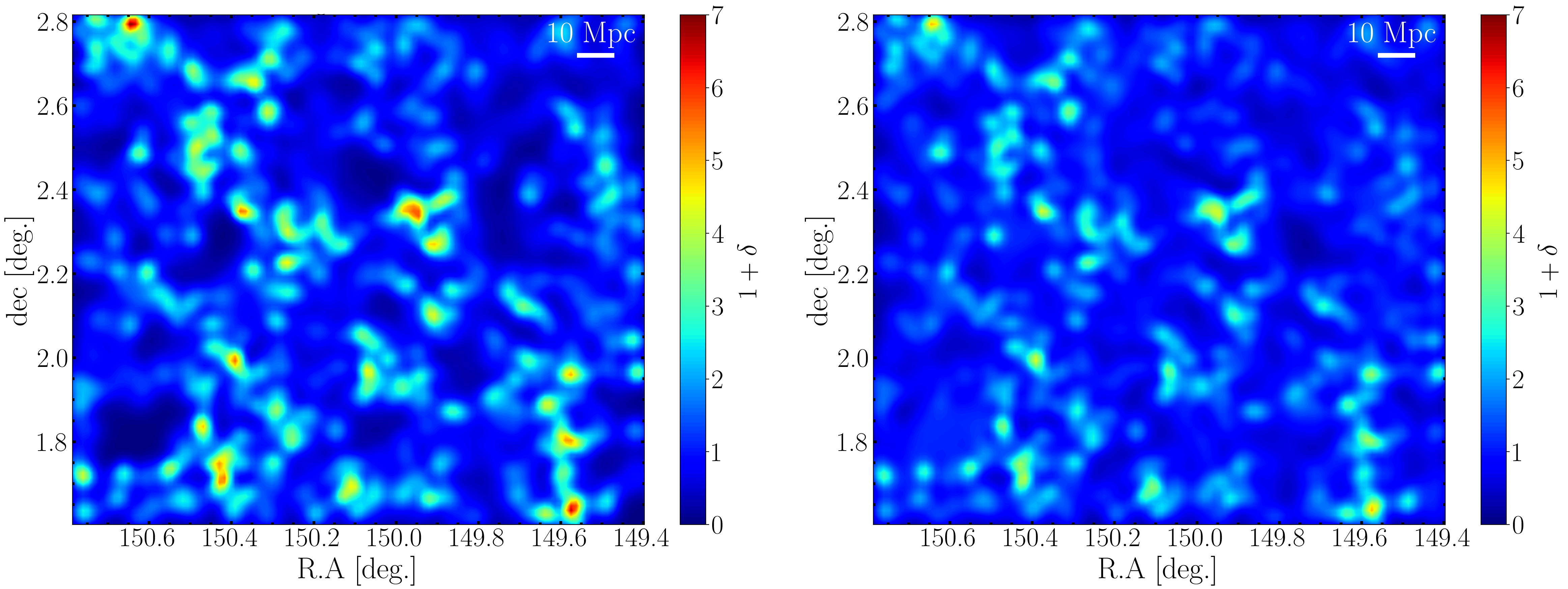
Figure 4: Density maps reconstructed for $z=2.93$. Left: the density map without corrections for masked regions. Right: the corrected density map, incorporating corrections for masked regions by populating them with uniformly distributed artificial sources, resulting in a smoother density field, especially around large masked regions.

3.3 Weight Calculation

Once we determined the redshift slices we can calculate the weight of a galaxy g in the redshift slice s, denoted as $w^{g}_{s}$, which is the probability of galaxy g being in the redshift slice s. For simplicity, we use a Gaussian probability distribution to calculate these weights for most of the galaxies in the sample that have a single solution for their photo-$z$. We put the center of the Gaussian PDF on the estimated photo-$z$, with a standard deviation calculated using the 68% confidence interval of photo-$z$. Hence, $w^{g}_{s}$ can be calculated as

$$w^{g}_{s}=\int_{s}P_{G}(z;\mu=z_{g},\sigma=\Delta z)\,dz$$ (6)

where $z_{g}$ is the estimated photo-$z$ and integration domain is over sth redshift interval. This is the contribution of galaxy g to the density field of sth redshift slice (Equation 1). A fraction of sources have a second solution for their photo-$z$. This fraction increases monotonically with magnitude-cut on either $H$ or $K_{s}$ bands. With our choice of magnitude cut ($K_{s}\sim 24.5$), less than 7% of sources in our sample, would have a second solution with $P>5\%$ for their photo-$z$. For these sources, we calculate the weights using their $z$PDF.

Theoretically, all galaxies with a Gaussian probability distribution will have non-zero weights in all redshift slices. To reduce the computational time in the density estimation step, we only keep galaxies that have large enough weights, above a weight threshold of value $w_{th}=0.05$, in a redshift slice. Figure 2 shows the effect of different choices of $w_{th}$ on the sample. The upper panel shows the effective number of galaxies, a summation of all weights in a redshift slice, as a function of redshift. The black curve represents the original sample (without threshold on weights) which is plotted as a reference. A higher threshold decreases the effective number of galaxies in all redshifts. The middle panel shows the effective number of galaxies in each redshift slice divided by the effective number of galaxies in all slices. The lower panel shows the fraction of sources in the sample that enter the next step, or the factor by which the threshold on weights reduces the computation time. The choice of $w_{th}=0.05$ significantly shrinks the sample size in all redshift slices while minimally affecting the trend of galaxy distribution across the redshift range.

The upper panel in Figure 3 shows the distribution of galaxies as a function of redshift. The dark blue histogram represents the number of galaxies that have measured photo-$z$ within a redshift slice and the light blue histogram shows the distribution of galaxies that have weights above $w_{th}=0.05$ in each redshift slice. Vertical red lines between two panels show the centers of 135 redshift slices. The bottom panel in Figure 3 shows the uncertainty of photo-$z$s (half of the $68\%$ confidence interval of calculated photo-$z$) as a function of redshift. The red dashed line shows the median of redshift uncertainties in each redshift slice.

3.4 Masked Regions

COSMOS2020 flags objects that are in the regions covered/affected by bright stars in the HSC survey (FLAG_HSC), and by bright stars in the legacy Supreme-cam data (FLAG_SUPCAM). These objects are affected by the fluxes of nearby stars or other artifacts. (Coupon et al., 2017) provide bright star masks from the HSC-SSP PDR2 which is used to flag objects in the vicinity of these sources (red circles in Figure 1). Moreover, artifacts in the Supreme-Cam images are masked using the same mask as in COSMOS2015 (Weaver et al., 2022). Approximately 18% of sources are located within these masked regions, where measurements (photometry and SED fitting) are not reliable (Weaver et al., 2022). This fraction of sources does not enhance our statistical conclusions and might introduce more uncertainties. Consequently, they are not used in this study.

Figure 5: This figure shows the steps taken in the construction of the density map for a redshift slice centered at $z=1.881$. Upper left: distribution of sources that have weights above $w_{th}$. Upper middle: uniformly distributed artificial sources populated in the masked regions. Upper right: actual galaxies combined with artificial points. Sources in all upper panels are colored by weight. Lower left: actual/artificial sources colored by adaptive bandwidth. Lower middle: the combination of actual/artificial sources colored by the edge correction factor. Lower right: final density map. Contours are placed at 1.5 and 2.5 levels.

Removing the flagged sources leads the density estimator to underestimate the densities around masked regions. To account for this error, we populate the masked regions with a uniform distribution of “artificial” sources that meet the following two criteria:

• The number density of the “artificial” sources is equal to the average number density of galaxies (actual data) in the field, excluding the masked area:

  $$\bar{n}=\frac{\sum_{g}w^{g}_{s}}{A_{\text{field}}-A_{\text{masked}}}$$ (7)

  Where $A_{\text{field}}$ and $A_{\text{masked}}$ are the whole field and masked area, respectively.

• We choose an identical weight for all these artificial sources such that they do not change the average weight of all galaxies in the redshift slice:

  $$\bar{w}=\frac{\sum_{g}\,w^{g}_{s}}{N_{g}^{s}}$$ (8)

  where $N_{g}^{s}$ is the number of actual galaxies in the $s$th redshift slice.

Figure 4 presents a comparison between the constructed density field before and after performing corrections for this effect at $z=2.93$. It is clear how the constructed density field around these masked regions will be affected by the lack of sources in these regions if we do not implement corrections.

3.5 Bandwidth Selection

The next step is to choose a bandwidth representing the scale to which the kernel smooths the field, termed “global bandwidth”. An optimum bandwidth should be chosen based on the number density of sources in each $z$-slice and the extent to which they are clustered: a larger bandwidth results in an over-smoothed field and consequently less information about fine structures and a smaller bandwidth leads to an under-smoothed field with high variance and uncorrelated small scale structures. Selection of the optimum bandwidth is a challenging part of the wKDE. Several methods have been suggested to find the optimum bandwidth. It can be motivated by the physical size of structures of interest in the study. For instance, (Darvish et al., 2015) adopt a constant global bandwidth of physical length $h=0.5\,\text{Mpc}$ for all redshifts, which corresponds to the characteristic size, $R_{200}$, for X-ray clusters and groups in the COSMOS field. (Chartab et al., 2020) employ the leave-one-out Likelihood Cross-Validation (LCV) method (Hall, 1982) to find the optimum global bandwidth for each $z$-slice.

As we perform the analysis in a broad redshift range ($0.4<z<6$), adopting a constant physical size for the kernel bandwidth will be an oversimplification and leads us to an unfair estimation of the density field: a fixed bandwidth that performs well at lower redshifts is not our best choice at higher redshifts where the source distribution is more sparse. Therefore, we need to consider the varying number of sources in each redshift slice to set the appropriate bandwidths. We use the LCV method (Hall, 1982; Chartab et al., 2020) to find the most likely bandwidth in each $z$-slice, $b_{s}$, given the distribution of sources with specified weights. The method involves a grid search on a range of bandwidths, calculating the likelihood of each candidate bandwidth, and finding the bandwidth that yields the highest likelihood value as the optimal bandwidth. The outcome of this method, $b_{s}$, is data-driven, without any presumption on the bandwidth size, and asymptotically minimizes an integrated squared error in the estimated density (Chartab et al., 2020; Hall, 1982):

$$\text{LCV}(b_{s})=\frac{1}{N}\sum_{k=1}^{N}\log\sigma_{-k}(\textbf{X}_{k})$$ (9)

where N is the total number of sources in the field and $\sigma_{-k}(\textbf{X}_{k})$ is the calculated density at position $\textbf{X}_{k}$ leaving the kth data point out of the sample (if we do not remove the kth data point, the optimal b would be zero).

Table 1: Density field measurements for sources in COSMOS2020 catalog.

ID	photo-$z$	R.A.	Dec.	density contrast	Comoving density	Physical density	SF/Q
		(deg.)	(deg.)	($\delta$)	($\text{Mpc}^{-3}$)	($\text{Mpc}^{-3}$)
964384	1.6049	149.97682	2.4550	-0.0438	0.0011	0.020	1
964388	1.9782	150.44084	2.5423	0.1876	0.0016	0.043	0
964392	0.8828	149.92698	2.3762	2.7537	0.0317	0.213	1
964393	3.4578	149.97589	2.4575	0.6914	0.0003	0.030	1
964394	0.4715	150.22125	1.7919	0.4254	0.0163	0.051	1

Next, we determine a local adaptive bandwidth for each point, $b_{i}$, adjusting it according to the clustering level in the surrounding area. In regions with higher clustering, a smaller bandwidth is used for better resolution of smaller structures. Adaptive bandwidth prevents over-smoothing in dense areas and accommodates broader correlations in sparse regions. We calculate $b_{i}$ as (Abramson, 1982; Darvish et al., 2015; Chartab et al., 2020):

$$b_{i}=b\left(\frac{\sigma(X_{i})}{g}\right)^{-\alpha}$$ (10)

where $g$ is the geometrical mean of the estimated surface density, $\sigma(X_{i})$, for all sources in the field:

$$\log g=\frac{1}{N}\sum_{i}^{N}\log\sigma(X_{i})$$ (11)

Where $\alpha$ is a constant sensitivity parameter ranging from 0 to 1 and can be determined through simulation. We choose $\alpha=0.5$, as it has minimal impact on the outcome.

3.6 Edge Correction

The wKDE algorithm is effective in areas away from the edges of the field. However, due to the lack of sources outside the surveyed area, it tends to underestimate density near the edges. This affects only a minor portion of our sources, given the COSMOS wide area. In this section, we implement a correction to address this error. Several methods have been developed to reduce the edge effect, e.g., the reflection method (Schuster, 1985), the boundary kernel method (Müller, 1991), the transformation method (Marron & Ruppert, 1994), and renormalization method (Jones, M. C., 1993). In this study, we use the re-normalization method: The expectation value of the density field at point $X_{0}$, up to the first order, is

$$\mathbb{E}\sim\sigma^{s}_{\text{True}}(X_{0})\int_{S}K(X_{i};X_{0})$$ (12)

where $\sigma_{\text{True}}^{s}(X_{0})$ is the true value of the density field at position $X_{0}$ and the integration domain is over the whole field with area S. This integral tends to one if $X_{0}$ is far enough from the edges; tends to $\sim 0.5$ for a point which is right on one of the edges, and is $\sim 0.25$ for a point on one of the four corners. Therefore, a reasonable choice for the correction of the edge effect is (Chartab et al., 2020)

$$\sigma^{s}_{\text{corrected}}=\sigma^{j}(X_{0})n(X_{0})$$ (13)

where $n(X_{0})$ is defined as follows:

$$n^{-1}(X_{0})=\int_{S}K(X_{i};X_{0})$$ (14)

The correction factor, $n$, ranges from 1 for a point far from the edges to $\sim 4$ right at one of the corners.

Figure 6: Constructed density maps for three different redshift slices. They are centered at $z=0.722$, $z=0.925$, and $z=2.473$, respectively from the left. We see the filamentary structure known as “COSMOS Wall” in the left panel (Iovino et al., 2016). In the middle panel, we see another elongated structure at $0.92$. In the right panel, we see a symmetric overdensity of $(1+\delta)\gtrsim 4$ in the bottom-right corner of the field. Contours are placed at density enhancement level $(1+\delta)\sim 2$.

3.7 Density Map Construction

Figure 5 shows all the steps to construct the density maps in one of the 135 redshift slices spanning $0.4<z<6$. Here we summarize the whole process:

1. Top-Left. We calculate the weight for all galaxies in a redshift slice, either assuming a Gaussian zPDF or by using the actual redshift PDF for those that have two solutions for their photo-$z$ with $P>5\%$.

2. Top-Middle. We populate the masked regions with artificial sources of uniform distribution and combine them with the actual galaxies (Top-Right).

3. Bottom-Left. We find the optimum global bandwidth in each redshift slice, $b(s)$, using the leave-one-out Likelihood cross-validation method (Equation 9) and then calculate the adaptive bandwidth (Equation 10) at the position of each galaxy.

4. Bottom-Middle. We calculate the correction factor for all sources to compensate for the edge effect using the global bandwidth calculated in step 3.

5. Bottom-Right. The last step is to construct the over-density maps and calculate the densities for all sources. Over-densities are calculated using the background surface density, $\sigma_{\text{median}}$, defined as the median of the reconstructed surface density field in each redshift slice.

   $$1+\delta=\frac{\sigma}{\sigma_{\text{median}}}$$ (15)

   With our choice of kernel bandwidth (calculated from LCV), $\sigma_{\text{median}}$, is almost constant at all redshifts. We selected the median to define the background density, minimizing bias from outliers.

Comoving density, $\rho_{\text{comoving}}$, is defined as the number of galaxies in $1\,\text{Mpc}^{3}$ of comovong space. We calculate the comoving density as $\rho_{\text{comoving}}=(1+\delta)\bar{\rho}$, where $\bar{\rho}$ is the average number density of galaxies in $s$th redshift slice:

$$\bar{\rho}=\frac{\sum_{g}w_{s}^{g}}{\mathbb{V}_{s}}$$ (16)

Where $\mathbb{V}_{s}$ is the comoving volume associated with the $s$th redshift slice and $\sum_{g}w_{s}^{g}$ is the effective number of galaxies in the desired redshift slice.

Table 1 presents a portion of the full density catalog, including ID, photo-$z$, R.A., and Dec. (from COSMOS catalog); and the measured density contrast, comoving, physical density, and star-forming/quiescent flag (explained in Section 4.2). The full electronic density catalog is published in its entirety.

4 Results & Discussion

In this section, we present the results of density estimation and utilize them to study the environmental dependence of star formation activity. Our analysis involves two distinct galaxy groups: an overall sample encompassing both star-forming and quiescent galaxies, and a sample of only star-forming galaxies. Additionally, we explore the redshift evolution of this relationship by dividing the entire sample into different cosmic epochs (redshift intervals).

4.1 Large Scale Structures (Density Maps)

We release overdensity maps along with the spatial distribution of weighted sources for 135 $z$-slices spanning $0.4<z<6$. The full set of maps is available in animated format. Three examples are shown in Figure 6. In the left panel, we see the filamentary structure at $z\sim 0.73$ known as “COSMOS Wall” studied in (Iovino et al., 2016). In the middle panel, we observe another elongated structure at $z\sim 0.92$. The right panel shows a symmetric overdensity of $(1+\delta)\gtrsim 4$ in the bottom-right corner of the field. Contours are placed at density enhancement level $(1+\delta)\sim 2$.

4.2 Environmental Dependence of SFR and its Redshift Evolution

To study the redshift evolution of SFR/sSFR-density, we divide our sample into mass-complete sub-samples in 6 redshift intervals. The choice of magnitude cut $K_{s}\sim 24.5$ and other selection criteria introduced in Section 2, result in a magnitude-limited sample that is distinct from the original COSMOS2020 catalog. In a magnitude-limited sample, the minimum stellar mass we have observations for depends on both redshift and stellar mass-to-light ratio. To obtain mass-complete sub-samples in each redshift interval, we follow the method outlined in (Pozzetti et al., 2010; Ilbert et al., 2013). We first re-scale the stellar mass of galaxies to a limiting mass, $M_{\text{lim}}$, which is the mass that a galaxy would have at its redshift if we shift its apparent magnitude to the limiting magnitude of the survey or, in our case, the magnitude-cut $K_{s}\sim 24.5$. All types of galaxies above this mass limit are considered to be brighter than the magnitude cut, and potentially observable. The mass re-scaling relation is $\log(M_{\text{lim}}/M_{\odot})=\log(M/M_{\odot})+0.4(K_{s}-K_{s,\text{cut}})$, where $M$ is the estimated stellar mass of the galaxies reported by The Farmer-LePhare combination. A constant stellar mass-to-light ratio is presumed in this relation.

At each redshift interval, the final completeness limit $M_{\text{comp}}$, corresponds to the mass below which 95% of the galaxies’ re-scaled masses are populated. This is to ensure that for any subset of galaxies with masses above this limit, not more than 5% of them could be missed in the lower mass regime. In each interval, less massive (fainter) galaxies that appear at the low redshift end, might be absent at the high redshift end, introducing biases toward more massive galaxies. To minimize this bias, in each redshift interval, we calculate the completeness limit at the high redshift end of the interval. Figure 7 shows the distribution of stellar masses versus redshift for our sample. The blue solid line is the mass-completeness fitting function introduced in (Weaver et al., 2022) for the whole COSMOS2020 catalog plotted here as a reference. Red boxes show the areas that contain galaxies in our 6 sub-samples, obtained by this approach. Orange dots show the completeness limit we calculated in redshift bins of width 0.1 and the dashed orange line shows the corresponding polynomial fitting function in $(1+z)$.

Figure 7: Stellar mass distribution of sources in the sample across the whole redshift range. Red boxes show the boundaries of 6 mass-completeness samples chosen following the method outlined in (Pozzetti et al., 2010). Properties of these mass-complete samples are summarized in the first three columns of table 2. Orange dots are completeness limits calculated in redshift bins of width $0.1$ and the dashed orange line is the corresponding polynomial fitting function in $(1+z)$. The blue curve is the mass-completeness limit of the original catalog introduced in (Weaver et al., 2022), plotted as a reference.

This selection of redshift intervals ensures a substantial number of galaxies in each group. The properties of resulted sub-samples, including redshift range, mass-completeness limit, and sample sizes are given in the first three columns of Table 2. While we have constructed the density maps for the full redshift range $0.4<z<6$, and we report environmental densities out to $z\sim 5$, we limit the analysis in this part to sources within the range $0.4<z<4$. At $4<z<6$, the number of sources in mass-complete samples becomes significantly low ($<300$) which makes any statistical conclusion unreliable.

In total, 97247 galaxies are used in the mass complete sub-samples out to $z\sim 4$. We then use the rest-frame color-color (NUV-$r$ vs. $r$-J) diagram to identify quiescent galaxies in each bin using the classification criteria introduced by (Ilbert et al., 2013): galaxies with a rest-frame color NUV-$r>3.1$ and NUV-$r>3$($r$-J)$+1$ are flagged as quiescent. Figure 8 shows the population of star-forming and quiescent galaxies in each redshift interval all colored by their SFR.

Figure 9 presents the SFR and sSFR as a function of environmental density for two samples: 1) the overall sample (columns 1 & 3), and 2) the sample of only star-forming galaxies (columns 2 & 4). Colorbars correspond to the population in pixels. At lower redshifts ($0.4<z\lesssim 1.5$), a significant population of sources is found in high-density environments ($\log(1+\delta)\sim 1$). Conversely, at higher redshifts ($1.5\lesssim z<4$), sources are mostly populated in low/intermediate densities ($\log(1+\delta)\lesssim 0.6$). In addition, we observed a population of low-SFR/sSFR sources at intermediate densities ($-0.2\lesssim\log(1+\delta)\lesssim 0.8$) in columns 1 and 3 (the overall samples). Notably, at $z\lesssim 1.5$, most of these sources vanish in columns 2 and 4, where we exclude quiescent galaxies from our sample. This is attributed to the fact that, among galaxies in low/intermediate density environments, those with low SFR/sSFR are mainly quiescent galaxies. However, this trend lessens at higher redshifts ($1.5<z<4$): there is still a considerable population of “passive” galaxies at low/intermediate densities ($-0.2\lesssim\log(1+\delta)\lesssim 0.8$), even after excluding quiescent galaxies. When interpreting these findings, it is crucial to consider the class imbalance between star-forming and quiescent galaxies at all redshift intervals (Figure 8) and biases toward bright/massive objects at higher redshifts. Furthermore, it should be noted that the COSMOS field, particularly at lower redshifts ($z\lesssim 2$), does not have substantial overdensities compared to other low-redshift surveys or those that are designed to target massive LSS (e.g., SDSS, York et al. 2000, EdisCS, White et al. 2005; GOGREEN, Balogh et al. 2017; ORELSE, Lubin et al. 2009). As a result, some severe environmental effects, may not be observed within the range of environments we have here ($-0.2\lesssim\log(1+\delta)\lesssim 1.1$).

Figure 8: NUV-$r$ vs. $r$-J color-color diagrams and the criteria used to identify quiescent and star-forming galaxies (solid lines) in the 6 mass-complete samples chosen within $0.4<z<4$. Galaxies in the regions defined as NUV-$r>3.1$ and NUV-$r>3$($r$-J)$+1$ are identified as quiescent (Ilbert et al., 2013).

To better understand these trends, we present the corresponding binned statistics in Figure 10. Average SFR and sSFR are calculated in bins of density, with error bars indicating the standard error of mean values. For both overall and star-forming samples, the SFR-density and sSFR-density trends are almost the same. A considerable difference between SFR-density and sSFR-density dependence is that the average SFR of galaxies increases with increasing redshift, while the average sSFR does change significantly at different redshifts. The notable decrease in SFR from higher to lower redshifts is related to the decline in the global star formation density of the universe after $z\sim 2-3$ (Sobral et al., 2012; Khostovan et al., 2015).

4.2.1 Overall Sample (Star-Forming and Quiescent)

The upper panels in Figure 10 show the average SFR/sSFR as a function of redshift for the “overall” sample. We see a clear anti-correlation between SFR/sSFR and density up to $z\sim 1.1$. In the lowest redshift interval ($0.4<z<0.8$), SFR decreases by a factor of $\sim 150$ as the density increases from $\delta\sim-0.5$ to $\delta\sim 10$, and for the redshift interval $0.8<z<1.1$ the SFR decreases by a factor of $\sim 10$ across the same range of density. These low-redshift trends are generally in agreement with majority of previous studies (e.g., Patel et al. 2009; Scoville et al. 2013; Darvish et al. 2016; Chartab et al. 2020) and are almost well-established. At intermediate redshifts, $1.1<z<2$, SFR/sSFR become almost independent of the environment. The same result is reported in (Darvish et al., 2016) for $1.1<z<3.1$ and in (Scoville et al., 2013) for $z\gtrsim 1$, but (Chartab et al., 2020) report an anti-correlation at all redshifts out to $z\sim 3.5$. As noted in Section 1, the main controversy centers on trends at higher redshifts ($z\gtrsim 1$). At $2<z<4$, we see the reversal of the SFR/sSFR-density relation. For both samples, at $2<z<3$ and $3<z<4$, SFR increases by a factor of $\sim 10$ as the density increases from $-0.4$ to $\sim 5$. As a result of the negative correlation between SFR-density, the decline in the average SFR is $1.1$ dex at low-density environments ($\delta\sim-0.5$), whereas, in the higher densities ($\delta\sim 5$), SFR decline is $\sim 2.8$ dex since $z\sim 4$ to the lowest redshift. The situation is different in sSFR-density trends: while at low-density environments there is no significant change in average sSFR-density relation at different redshifts, there is a significant decline ($\sim 3$ dex) in high-density end ($\delta\sim 3$) since $z\sim 4$ to the lowest redshift bin.

Table 2: Properties of mass-complete samples and correlation coefficients

Redshift Range	$\log(\text{M}_{min}/\text{M}_{\odot})$	Sample Size	correlation coeff. (SFR vs. density)		correlation coeff. (sSFR vs. density)
			(SF+Q)	SF	(SF+Q)	SF
$0.4<z<0.8$	8.791	26548	-0.022	0.044	-0.093	-0.038
$0.8<z<1.1$	9.163	23561	-0.011	0.061	-0.090	-0.038
$1.1<z<1.5$	9.479	22643	0.027	0.050	-0.032	-0.017
$1.5<z<2$	9.811	13099	-0.020	0.002⋆	-0.038	-0.020
$2<z<3$	10.122	9234	0.073	0.075	0.040	0.046
$3<z<4$	10.357	2162	0.090	0.094	0.150	0.144

^⋆ $P>5\%$

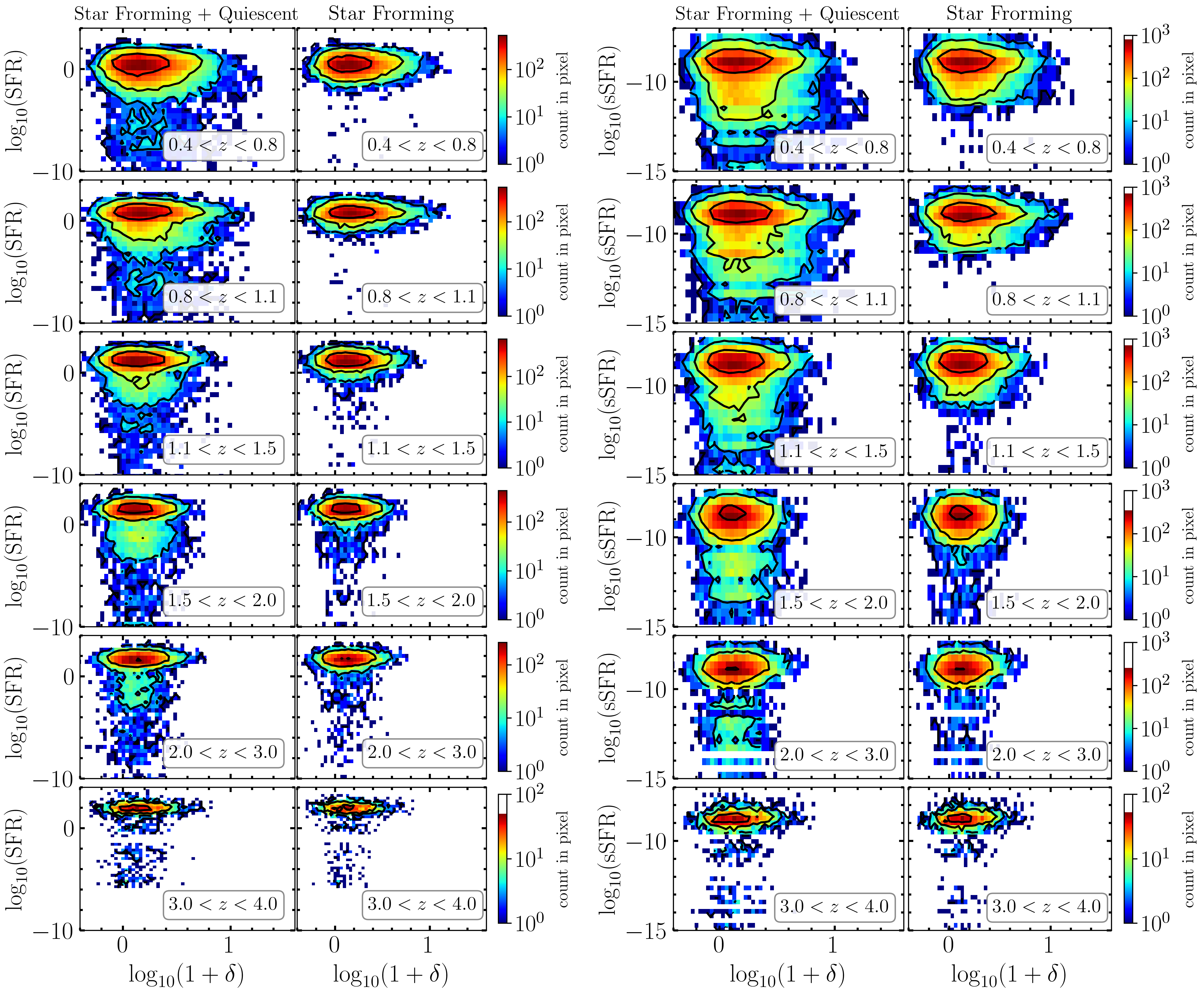
Figure 9: Two columns on the left show SFR vs. environmental density in 6 redshift intervals (column 1: the overall sample; column 2: the star-forming sample). Two columns on the right show sSFR vs. environmental density in 6 redshift intervals (column 3: the overall sample; column 4: the star-forming sample). Colorbars correspond to the population in each pixel and the contours are placed at 3 equally spaced levels between the minimum and maximum population per pixel in each plot.

The reversal of SFR-density trends has been reported in several studies. (Elbaz, D. et al., 2007) observe the reversal of the SFR-density relation at $z\sim 1$. Utilizing a set of spectroscopic observations (Lemaux et al., 2022) report a positive correlation between the average SFR and galaxy overdensity in the early universe ($2<z<5$). These relations between SFR-density are partly due to the correlation between SFR and stellar mass. However, the anti-correlation between sSFR and density implies that environmental density directly influences the star formation activity of galaxies. This might be due to the greater availability of gas content in high-density environments, potentially leading to increased star formation rates at the initial stages of galaxy evolution ($z>2$) for galaxies in these rich environments.

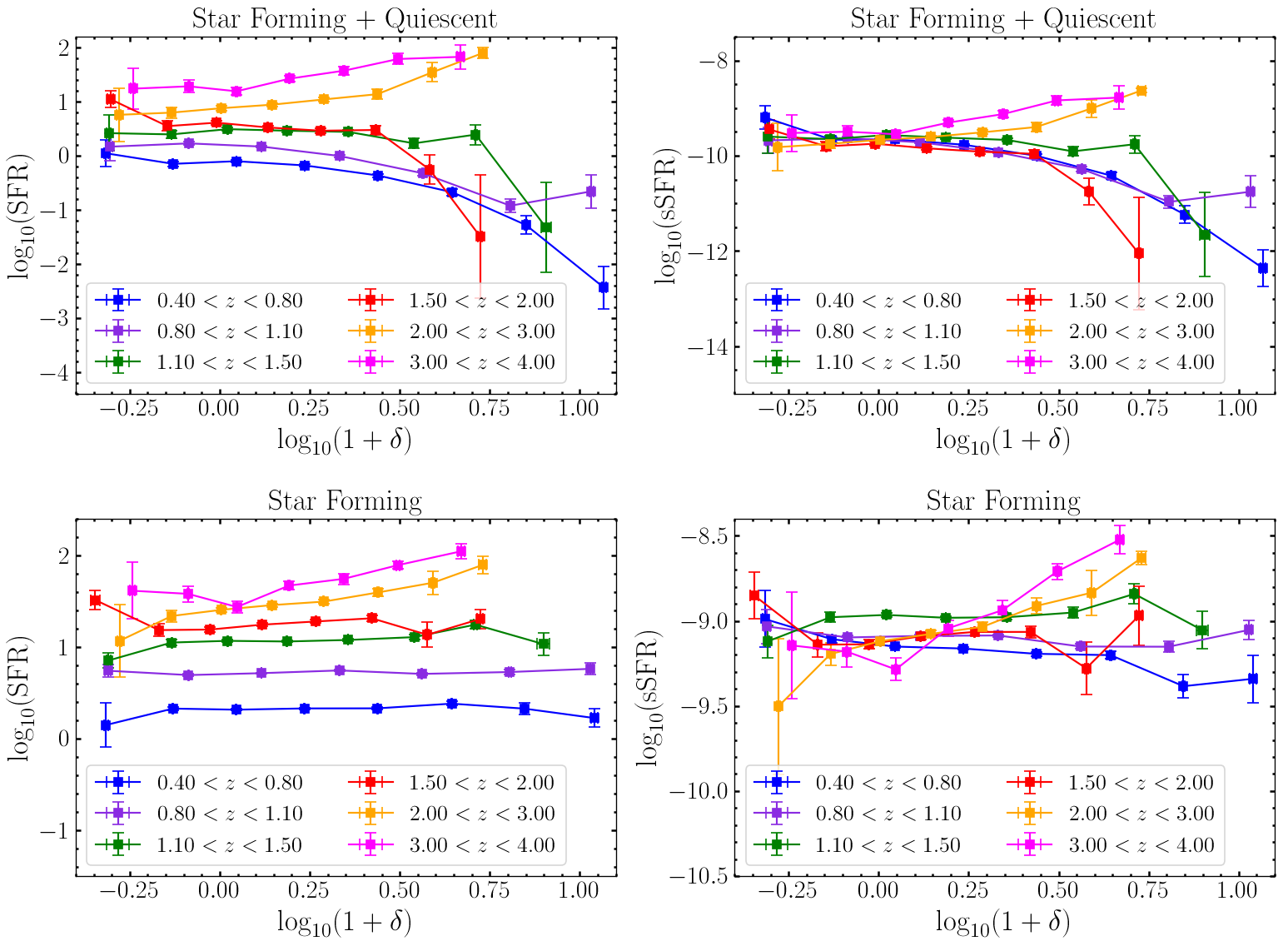
Figure 10: Average SFR (left) and sSFR (right) are plotted versus density enhancement in each redshift interval. Top: Relation for all the galaxies (star-forming and quiescent). Bottom: the same relation for star-forming galaxies. Out to $z\sim 1.1$, the median SFR and sSFR decrease with increasing density enhancement. At intermediate redshifts, $1.1<z<2$ the SFR/sSFR in the mixed sample (star-forming and quiescent) becomes almost independent of the density. At higher redshifts ($2<z<4$) there is a positive correlation between star formation activity and the environment. When considering only star-forming galaxies (bottom panels) the anti-correlation for both SFR and sSFR transforms to a flat trend at low/intermediate redshifts and a positive correlation at higher redshifts.

4.2.2 Star-Forming Sample

The bottom panels in Figure 10 show the average SFR (bottom left) and average sSFR (bottom right) as a function of density for a sample of star-forming galaxies. At lower redshifts $z\lesssim 2$ both SFR and sSFR are almost independent of environment. We observe a decline of SFR from higher to lower redshifts across the whole density range. At higher redshifts ($z\gtrsim 2$) there is a positive correlation between SFR and density: SFR increases by a factor of $\sim 8$ as density increases from $-0.5$ to $4.5$. Considering the uncertainties, there is no clear correlation between sSFR and density for the star-forming sample.

4.3 Correlation Coefficients

To quantify the statistical significance of our findings, we calculated the “Spearman” correlation coefficient for the reported trends in both overall and star-forming samples. A correlation coefficient close to 1 indicates a strong positive correlation, a coefficient close to 0 indicates no significant correlation, and a coefficient close to -1 indicates a strong negative correlation. The presumed correlation does not need to be linear. Table 2 summarizes the properties of mass-complete samples at 6 redshift intervals, along with the Spearman correlation coefficient. For the second redshift interval ($0.8<z<1.1$) in the overall sample and for the fourth redshift interval ($1.5<z<2$) in the star-forming sample, the P-values are 0.02 and 0.7, respectively. The former is still $<5\%$ but large compared to other P-values and the latter implies that correlations observed in $1.5<z<2$ are not statistically reliable. All other P-values associated with Spearman correlation coefficients reported in Table 2 are less than $10^{-4}$. While the small correlation coefficient values might seem inconsistent with the binned statistics shown in Figure 10, one should note that these correlation coefficients are calculated for all sources in each redshift interval and are highly affected by the outliers due to the large scatter of data (Figure 9). Other than that, these coefficients are in agreement we see in trends (Figure 10), and their small P-values indicate the reliability of correlations.

5 Summary

We use a magnitude-limited ($K_{s}<24.5$) sample of galaxies in the COSMOS2020 catalog to reconstruct the density maps at $0.4<z<6$. We choose 135 redshift slices of constant comoving width $35\,h^{-1}\,\text{Mpc}$ and assign weights to galaxies in all redshift slices using their $z$PDF. We calculate densities adopting the weighted Kernel Density Estimation method, with the choice of von Mises-Fisher kernel, and improve our density estimation by correcting the “edge effect” and masked regions.

We release a publicly available catalog of calculated environmental densities for nearly $\sim 200\,k$ galaxies, along with an animated version of density maps out to $z\sim 6$ which can be used to identify LSS across this redshift range. To investigate the relation between the star formation activity of galaxies (SFR/sSFR) and environmental density, and the redshift evolution of this relation, we present the corresponding binned statistics in 6 mass-complete sub-samples at different redshift intervals (details in Table 2). Our findings show that for the overall sample, the median of SFR and sSFR decreases with increasing density out to $z\sim 1.1$. This negative correlation is consistent with many previous studies in this regard (Elbaz, D. et al., 2007; Scoville et al., 2013; Darvish et al., 2016; Chartab et al., 2020). There is a transition range at $1.1<z<2$ in which there is no significant correlation between SFR/sSFR and density. At higher redshifts ($2<z<4$), where there are more debates around the SFR/sSFR-density relation, we see a positive correlation between SFR/sSFR and the density (the reversal of trends). For the star-forming sample, SFR/sSFR are almost independent of the environment out to $z\sim 2$. Across the whole density range, we observe the decline of SFR from higher to lower redshifts, while sSFR remains unchanged. At higher redshifts ($z\gtrsim 2$) we observe a positive correlation in the SFR-density relationship. The strength of all these correlations is listed as the “Spearman” correlation coefficient in the table 2. One should note that these coefficients are calculated for the whole data in each case and their small values are due to the large scatters that can be seen in Figure 9, however, very small P-values in almost all of the cases suggest that the correlations hold statistical significance. Correlations between SFR-density are partly due to the SFR-stellar mass relation, but sSFR trends show that even star formation activity per unit mass is affected by the environment in the overall sample. To have a more accurate understanding of these trends at high redshifts, we still need to acquire deeper observations, more accurate photometric measurements, and as a result, more accurate SED fitting: at higher redshifts, we are always biased toward more massive objects and wKDE or any other density estimation method is extremely sensitive to the accuracy of $z$PDF which broadens at higher redshifts, due to the observational limits. In addition, our statistical conclusions about SFR/sSFR-density relation are highly dependent on the accuracy of SED fitting outputs. The accuracy of properties derived from SED-fitting depends on various factors including the dust content of the galaxies. For instance, extremely dusty star-forming galaxies might have their SFR underestimated if their dust obscuration is not adequately accounted for in the SED models. At higher redshifts, particularly around $z\sim 2-3$, where the contribution of dusty star-forming galaxies to the overall SFR budget is significant, this bias could potentially impact the observed SFR-density relations.

6 Acknowledgments

We are grateful to the anonymous referee for their helpful comments that greatly improved the quality of this work. Some of the data used in this study were obtained at the W.M. Keck Observatory, which is operated as a scientific partnership among the California Institute of Technology, the University of California, and the National Aeronautics and Space Administration. The Observatory was made possible by the generous financial support of the W.M. Keck Foundation. The authors wish to acknowledge the profound cultural role of the Maunakea’s summit within the indigenous Hawaiian community. This work is based on data products from observations made with ESO Telescopes at the La Silla Paranal Observatory under ESO program ID 179.A-2005 and on data products produced by CALET and the Cambridge Astronomy Survey Unit on behalf of the UltraVISTA consortium. This work is based in part on observations made with the NASA/ESA Hubble Space Telescope, obtained from the Data Archive at the Space Telescope Science Institute, which is operated by the Association of Universities for Research in Astronomy, Inc., under NASA contract NAS 5-26555. ST was partially supported by the NSF award 2206813 during this work.

References

- A. Guillamón & Ruiz (1998) A. Guillamón, J. N., & Ruiz, J. 1998, Communications in Statistics - Theory and Methods, 27, 2123, doi: 10.1080/03610929808832217
- Abramson (1982) Abramson, I. S. 1982, The Annals of Statistics, 10, 1217 , doi: 10.1214/aos/1176345986
- AnsariFard et al. (2022) AnsariFard, M., Baghkhani, Z., Ghodsi, L., et al. 2022, Monthly Notices of the Royal Astronomical Society, 512, 5165, doi: 10.1093/mnras/stac256
- Arnouts et al. (2002) Arnouts, S., Moscardini, L., Vanzella, E., et al. 2002, MNRAS, 329, 355, doi: 10.1046/j.1365-8711.2002.04988.x
- Bai et al. (1988) Bai, Z. D., Rao, C. R., & Zhao, L. C. 1988, Journal of Multivariate Analysis, 27, 24, doi: https://doi.org/10.1016/0047-259X(88)90113-3
- Baldry et al. (2006) Baldry, I. K., Balogh, M. L., Bower, R. G., et al. 2006, Monthly Notices of the Royal Astronomical Society, 373, 469, doi: 10.1111/j.1365-2966.2006.11081.x
- Balogh et al. (2004) Balogh, M. L., Baldry, I. K., Nichol, R., et al. 2004, The Astrophysical Journal, 615, L101, doi: 10.1086/426079
- Balogh et al. (2017) Balogh, M. L., Gilbank, D. G., Muzzin, A., et al. 2017, MNRAS, 470, 4168, doi: 10.1093/mnras/stx1370
- Bamford et al. (2009) Bamford, S. P., Nichol, R. C., Baldry, I. K., et al. 2009, MNRAS, 393, 1324, doi: 10.1111/j.1365-2966.2008.14252.x
- Bardeen et al. (1986) Bardeen, J. M., Bond, J. R., Kaiser, N., & Szalay, A. S. 1986, ApJ, 304, 15, doi: 10.1086/164143
- Bond et al. (1996) Bond, J. R., Kofman, L., & Pogosyan, D. 1996, Nature, 380, 603, doi: 10.1038/380603a0
- Brammer et al. (2008) Brammer, G. B., van Dokkum, P. G., & Coppi, P. 2008, ApJ, 686, 1503, doi: 10.1086/591786
- Bruzual & Charlot (2003) Bruzual, G., & Charlot, S. 2003, MNRAS, 344, 1000, doi: 10.1046/j.1365-8711.2003.06897.x
- Capak et al. (2007) Capak, P., Abraham, R. G., Ellis, R. S., et al. 2007, The Astrophysical Journal Supplement Series, 172, 284, doi: 10.1086/518424
- Capak et al. (2011) Capak, P. L., Riechers, D., Scoville, N. Z., et al. 2011, Nature, 470, 233
- Casey et al. (2015) Casey, C. M., Cooray, A., Capak, P., et al. 2015, ApJL, 808, L33, doi: 10.1088/2041-8205/808/2/L33
- Catinella et al. (2013) Catinella, B., Schiminovich, D., Cortese, L., et al. 2013, MNRAS, 436, 34, doi: 10.1093/mnras/stt1417
- Cautun et al. (2014) Cautun, M., van de Weygaert, R., Jones, B. J. T., & Frenk, C. S. 2014, MNRAS, 441, 2923, doi: 10.1093/mnras/stu768
- Chartab et al. (2020) Chartab, N., Mobasher, B., Darvish, B., et al. 2020, The Astrophysical Journal, 890, 7, doi: 10.3847/1538-4357/ab61fd
- Colless et al. (2001) Colless, M., Dalton, G., Maddox, S., et al. 2001, MNRAS, 328, 1039, doi: 10.1046/j.1365-8711.2001.04902.x
- Cooper et al. (2008) Cooper, M. C., Newman, J. A., Weiner, B. J., et al. 2008, Monthly Notices of the Royal Astronomical Society, 383, 1058, doi: 10.1111/j.1365-2966.2007.12613.x
- Coupon et al. (2017) Coupon, J., Czakon, N., Bosch, J., et al. 2017, Publications of the Astronomical Society of Japan, 70, doi: 10.1093/pasj/psx047
- Cucciati et al. (2018) Cucciati, O., Lemaux, B. C., Zamorani, G., et al. 2018, A&A, 619, A49, doi: 10.1051/0004-6361/201833655
- Darvish et al. (2016) Darvish, B., Mobasher, B., Sobral, D., et al. 2016, ApJ, 825, 113, doi: 10.3847/0004-637X/825/2/113
- Darvish et al. (2015) Darvish, B., Mobasher, B., Sobral, D., Scoville, N., & Aragon-Calvo, M. 2015, The Astrophysical Journal, 805, 121, doi: 10.1088/0004-637x/805/2/121
- Darvish et al. (2020) Darvish, B., Scoville, N. Z., Martin, C., et al. 2020, The Astrophysical Journal, 892, 8, doi: 10.3847/1538-4357/ab75c3
- Dressler (1980) Dressler, A. 1980, ApJ, 236, 351, doi: 10.1086/157753
- Elbaz, D. et al. (2007) Elbaz, D., Daddi, E., Le Borgne, D., et al. 2007, A&A, 468, 33, doi: 10.1051/0004-6361:20077525
- Farouki & Shapiro (1981) Farouki, R., & Shapiro, S. L. 1981, The Astrophysical Journal, 243, 32, doi: 10.1086/158563
- Forrest et al. (2023) Forrest, B., Lemaux, B. C., Shah, E., et al. 2023, Monthly Notices of the Royal Astronomical Society: Letters, 526, L56, doi: 10.1093/mnrasl/slad114
- García-Portugués et al. (2013) García-Portugués, E., Crujeiras, R. M., & González-Manteiga, W. 2013, Journal of Multivariate Analysis, 121, 152, doi: https://doi.org/10.1016/j.jmva.2013.06.009
- Gisbert (2003) Gisbert, F. J. G. 2003, Empirical Economics, 28, 335, doi: 10.1007/s001810200134
- Grützbauch et al. (2011) Grützbauch, R., Conselice, C. J., Bauer, A. E., et al. 2011, Monthly Notices of the Royal Astronomical Society, 418, 938, doi: 10.1111/j.1365-2966.2011.19559.x
- Gunn & Gott (1972) Gunn, J. E., & Gott, III, J. R. 1972, The Astrophysical Journal, 176, 1, doi: 10.1086/151605
- Hall (1982) Hall, P. 1982, Biometrika, 69, 383, doi: 10.1093/biomet/69.2.383
- Hung et al. (2016) Hung, C.-L., Casey, C. M., Chiang, Y.-K., et al. 2016, The Astrophysical Journal, 826, 130, doi: 10.3847/0004-637X/826/2/130
- Ilbert et al. (2006) Ilbert, O., Arnouts, S., McCracken, H. J., et al. 2006, A&A, 457, 841, doi: 10.1051/0004-6361:20065138
- Ilbert et al. (2013) Ilbert, O., McCracken, H. J., Le Fèvre, O., et al. 2013, A&A, 556, A55, doi: 10.1051/0004-6361/201321100
- Iovino et al. (2016) Iovino, A., Petropoulou, V., Scodeggio, M., et al. 2016, 592, A78, doi: 10.1051/0004-6361/201527673
- Jones, M. C. (1993) Jones, M. C. 1993, Statistics and Computing, 3, 135, doi: 10.1007/BF00147776
- Kauffmann et al. (2004) Kauffmann, G., White, S. D. M., Heckman, T. M., et al. 2004, Monthly Notices of the Royal Astronomical Society, 353, 713, doi: 10.1111/j.1365-2966.2004.08117.x
- Kent (1982) Kent, J. T. 1982, Journal of the Royal Statistical Society. Series B (Methodological), 44, 71. http://www.jstor.org/stable/2984712
- Khostovan et al. (2015) Khostovan, A. A., Sobral, D., Mobasher, B., et al. 2015, Monthly Notices of the Royal Astronomical Society, 452, 3948, doi: 10.1093/mnras/stv1474
- Laigle et al. (2016) Laigle, C., McCracken, H. J., Ilbert, O., et al. 2016, The Astrophysical Journal Supplement Series, 224, 24, doi: 10.3847/0067-0049/224/2/24
- Lang et al. (2016) Lang, D., Hogg, D. W., & Mykytyn, D. 2016, The Tractor: Probabilistic astronomical source detection and measurement, Astrophysics Source Code Library, record ascl:1604.008. http://ascl.net/1604.008
- Lee et al. (2016) Lee, K.-G., Hennawi, J. F., White, M., et al. 2016, ApJ, 817, 160, doi: 10.3847/0004-637X/817/2/160
- Lemaux et al. (2018) Lemaux, B. C., Fèvre, O. L., Cucciati, O., et al. 2018, A&A, 615, A77, doi: 10.1051/0004-6361/201730870
- Lemaux et al. (2022) Lemaux, B. C., Cucciati, O., Fèvre, O. L., et al. 2022, A&A, 662, A33, doi: 10.1051/0004-6361/202039346
- Libeskind et al. (2018) Libeskind, N. I., van de Weygaert, R., Cautun, M., et al. 2018, MNRAS, 473, 1195, doi: 10.1093/mnras/stx1976
- Lubin et al. (2009) Lubin, L. M., Gal, R. R., Lemaux, B. C., Kocevski, D. D., & Squires, G. K. 2009, AJ, 137, 4867, doi: 10.1088/0004-6256/137/6/4867
- Mandelbaum et al. (2006) Mandelbaum, R., Seljak, U., Kauffmann, G., Hirata, C. M., & Brinkmann, J. 2006, MNRAS, 368, 715, doi: 10.1111/j.1365-2966.2006.10156.x
- Marron & Ruppert (1994) Marron, J. S., & Ruppert, D. 1994, Journal of the Royal Statistical Society: Series B (Methodological), 56, 653, doi: https://doi.org/10.1111/j.2517-6161.1994.tb02006.x
- McConachie et al. (2022) McConachie, I., Wilson, G., Forrest, B., et al. 2022, ApJ, 926, 37, doi: 10.3847/1538-4357/ac2b9f
- Moore et al. (1996) Moore, B., Katz, N., Lake, G., Dressler, A., & Oemler, A. 1996, Nature, 379, 613, doi: 10.1038/379613a0
- Müller (1991) Müller, H.-G. 1991, Biometrika, 78, 521, doi: 10.1093/biomet/78.3.521
- Newman et al. (2020) Newman, A. B., Rudie, G. C., Blanc, G. A., et al. 2020, ApJ, 891, 147, doi: 10.3847/1538-4357/ab75ee
- Parzen (1962) Parzen, E. 1962, The Annals of Mathematical Statistics, 33, 1065 , doi: 10.1214/aoms/1177704472
- Patel et al. (2009) Patel, S. G., Holden, B. P., Kelson, D. D., Illingworth, G. D., & Franx, M. 2009, ApJ, 705, L67, doi: 10.1088/0004-637X/705/1/L67
- Pavesi et al. (2018) Pavesi, R., Riechers, D. A., Sharon, C. E., et al. 2018, ApJ, 861, 43, doi: 10.3847/1538-4357/aac6b6
- Peng et al. (2010) Peng, Y.-j., Lilly, S. J., Kovač, K., et al. 2010, ApJ, 721, 193, doi: 10.1088/0004-637X/721/1/193
- Pozzetti et al. (2010) Pozzetti, L., Bolzonella, M., Zucca, E., et al. 2010, A&A, 523, A13, doi: 10.1051/0004-6361/200913020
- Sawicki et al. (2019) Sawicki, M., Arnouts, S., Huang, J., et al. 2019, Monthly Notices of the Royal Astronomical Society, 489, 5202, doi: 10.1093/mnras/stz2522
- Schlafly & Finkbeiner (2011) Schlafly, E. F., & Finkbeiner, D. P. 2011, ApJ, 737, 103, doi: 10.1088/0004-637X/737/2/103
- Schuster (1985) Schuster, E. F. 1985, Communications in Statistics - Theory and Methods, 14, 1123, doi: 10.1080/03610928508828965
- Scoville et al. (2013) Scoville, N., Arnouts, S., Aussel, H., et al. 2013, The Astrophysical Journal Supplement Series, 206, 3, doi: 10.1088/0067-0049/206/1/3
- Sobral et al. (2012) Sobral, D., Smail, I., Best, P. N., et al. 2012, Monthly Notices of the Royal Astronomical Society, 428, 1128, doi: 10.1093/mnras/sts096
- Sousbie (2011) Sousbie, T. 2011, MNRAS, 414, 350, doi: 10.1111/j.1365-2966.2011.18394.x
- Taylor (2008) Taylor, C. C. 2008, Computational Statistics & Data Analysis, 52, 3493, doi: 10.1016/j.csda.2007.11.003
- Vogelsberger et al. (2014) Vogelsberger, M., Genel, S., Springel, V., et al. 2014, Nature, 509, 177, doi: 10.1038/nature13316
- Wang et al. (2016) Wang, T., Elbaz, D., Daddi, E., et al. 2016, ApJ, 828, 56, doi: 10.3847/0004-637X/828/1/56
- Weaver et al. (2022) Weaver, J. R., Kauffmann, O. B., Ilbert, O., et al. 2022, The Astrophysical Journal Supplement Series, 258, 11, doi: 10.3847/1538-4365/ac3078
- Weaver et al. (2023) Weaver, J. R., Zalesky, L., Kokorev, V., et al. 2023, ApJS, 269, 20, doi: 10.3847/1538-4365/acf850
- White et al. (2005) White, S. D. M., Clowe, D. I., Simard, L., et al. 2005, A&A, 444, 365, doi: 10.1051/0004-6361:20042068
- Woo et al. (2012) Woo, J., Dekel, A., Faber, S. M., et al. 2012, Monthly Notices of the Royal Astronomical Society, 428, 3306, doi: 10.1093/mnras/sts274
- York et al. (2000) York, D. G., Adelman, J., Anderson, John E., J., et al. 2000, AJ, 120, 1579, doi: 10.1086/301513