Towards Context-Aware Domain Generalization: Representing Environments with Permutation-Invariant Networks

Abstract

In this work, we show that information about the context of an input $\mathbf{X}$ can improve the predictions of deep learning models when applied in new domains or production environments. We formalize the notion of context as a permutation-invariant representation of a set of data points that originate from the same environment/domain as the input itself. These representations are jointly learned with a standard supervised learning objective, providing incremental information about the unknown outcome. Furthermore, we offer a theoretical analysis of the conditions under which our approach can, in principle, yield benefits, and formulate two necessary criteria that can be easily verified in practice. Additionally, we contribute insights into the kind of distribution shifts for which our approach promises robustness. Our empirical evaluation demonstrates the effectiveness of our approach for both low-dimensional and high-dimensional data sets. Finally, we demonstrate that we can reliably detect scenarios where a model is tasked with unwarranted extrapolation in out-of-distribution (OOD) domains, identifying potential failure cases. Consequently, we showcase a method to select between the most predictive and the most robust model, circumventing the well-known trade-off between predictive performance and robustness.

1 Introduction

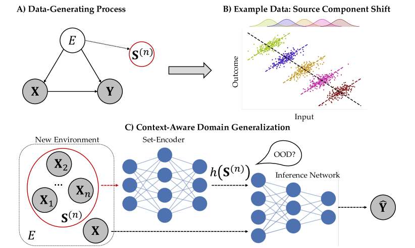
Figure 1: Conceptual sketch of our setup and approach. A) Data-generating process (DGP) that fulfills our criteria. We assume that the environment $E$ is a source node that is not caused by any system variable and that the relationship between $\mathbf{X}$ and $\mathbf{Y}$ varies with the environment. $\mathbf{S}^{(n)}$ is a set of $n$ IID inputs available in the new environment (i.e. context). B) The source component shift corresponding to the assumed DGP and example data coinciding with Simpson’s paradox. C) The workings of our approach in a test environment. A set-encoder generates a permutation-invariant representation $h(\mathbf{S}^{(n)})$ of the context. An inference network (e.g., a classifier) processes the representation along with the target input $\mathbf{X}$ and predicts the unknown outcome (e.g., label) of the target input. The set-representation can be combined with the input to reliably detect out-of-distribution (OOD) queries and prevent failure cases in domain generalization due to model misspecification.

Distribution shifts are the cause of many failure cases in machine learning [27, 32] and the root of various peculiar phenomena in classical statistics, such as Simpsons’ paradox [45, 57]. In this work, we employ permutation-invariant neural networks as set-encoders [15, 7] to improve the predictions of standard supervised models under distribution shift. Specifically, we consider training in the realm of Domain Generalization (DG), a setting where data from distinct environments is available for training and testing [39, 74].

For illustration, consider a probabilistic model $p(\mathbf{Y}\mid\mathbf{X})$ that classifies diseases $\mathbf{Y}$ from magnetic resonance (MR) images $\mathbf{X}$. Since MR images are not fully standardized, the classifier should work slightly differently for images acquired by different hardware brands. It thus makes sense to inform the classifier about the current environment $E$ (here: hardware brand) and extend it into $p(\mathbf{Y}\mid\mathbf{X},E)$. This raises two questions:

• Under which circumstances will the classifier $p(\mathbf{Y}\mid\mathbf{X},E)$ be superior to $p(\mathbf{Y}\mid\mathbf{X})$?

• How should $E$ be represented to maximize the performance gain?

The first question is important because there might exist a function $E=f(\mathbf{X})$ allowing the classifier $p(\mathbf{Y}\mid\mathbf{X})$ to deduce $E$ from the data $\mathbf{X}$. For example, $E$ might be inferred from the periphery of the given image, while $\mathbf{Y}$ depends on its central region. Then, no additional information is gained by passing $E$ explicitly, and both classifiers perform identically.

A straightforward answer to the second question is to distinguish environments by discrete labels. However, we argue that $E$ should be a continuous embedding. First, continuous embeddings can also be computed for new environments that have not been present in the training data. Second, when $p(\mathbf{Y}\mid\mathbf{X},E)$ receives a continuous $E$, it can potentially configure itself for unseen environments by interpolating between the training environments. And finally, discrete and continuous $E$ are equally informative for the known environments, ensuring no loss in information.

In the current work, we systematically investigate both questions, formalize three criteria when $p(\mathbf{Y}\mid\mathbf{X},E)$ is beneficial, and demonstrate how continuous embeddings $E$ can be learned from auxiliary data by means of set encoders (see Figure 1). Notably, two of these criteria are empirically testable using standard models and are shown to be necessary conditions for the success of the approach. First, we require that a single input alone is insufficient to deduce the originating environment (see Criterion 2.2). If this condition is not met, our model cannot possibly extract more information about the originating environment, compared to a standard model. Second, we require that, if the environment label is known by an oracle and given as an additional input to the standard model, its performance must improve (see Criterion 2.3). Otherwise, the set-based representation of the environment cannot possibly yield benefits. Notably, these two criteria are easy to verify and also met under the source component shift (see Section 2.6), which is a dataset shift that occurs in many scenarios [46].

When test environments are highly dissimilar to the training environments, all DG methods enter an extrapolation regime with unknown prospects of success and the potential to generate silent failures. While our approach is not exempt from this “curse of extrapolation”, it comes with a natural way to reliably detect novel environments in set-representation space and delineate its competence region [41]. Moreover, we propose a method to select between models that are specialized in the in-distribution (ID) setting vs. models that are robust to out-of-distribution (OOD) scenarios on the fly. Thus, we can overcome the notorious trade-off between ID predictive performance and robustness to distribution shifts [65, 42, 37]. Accordingly, we can adaptively select the most robust model in the OOD setting and the most predictive model in the ID setting, an approach we demonstrate on the ColoredMNIST data set [4]. In summary, our contributions are:

• We propose a novel approach to Domain Generalization (DG) that leverages context information from new environments in the form of learnable set-representations;

• We formalize the necessary and empirically verifiable conditions under which our approach can reap benefits from context information and improve on standard approaches;

• We perform an extensive empirical evaluation and show that we can reliably detect failure cases when the necessary criteria of our theory are not met, or when extrapolation is required.

2 Method

2.1 Notation

We denote inputs $\mathbf{X}\in\mathcal{X}$ and outputs as $\mathbf{Y}\in\mathcal{Y}$, without any strict requirements on the input and output spaces $\mathcal{X}$ and $\mathcal{Y}$, respectively. We treat the (unknown) domain label $E$ as a random variable and denote with $\mathbf{S}^{(n)}$ an i.i.d. sample (i.e., a set of further inputs) from the given domain. The domain label $E$ is only known during training time and unknown during inference.

2.2 General Idea

The key idea of our approach is to build models that utilize not only a singleton input $\mathbf{X}$ to predict a target $\mathbf{Y}$, but also information about the environment of $\mathbf{X}$ that can improve the prediction $\hat{\mathbf{Y}}$. Providing environmental information in the form of a one-hot label is hardly feasible, as it presupposes the exact number of possible environments to be known during training, and that we always know from which environment an input originates at inference time. Consequently, such an approach is doomed to fail when the test data originates from a novel or unknown environment.

To overcome this problem, we employ permutation-invariant neural networks to adaptively represent environmental information given a set of test inputs. We will first detail our approach and then discuss criteria under which we can expect to reap benefits from the additional set-representation. Afterwards, we explain the theoretical data-generating process that matches these criteria, providing insight into the distribution shifts for which our approach may prove advantageous in practice. Finally, we discuss the process of identifying new environments that demand extrapolation, potentially leading to failure cases.

2.3 Permutation-Invariant Neural Networks

As mentioned above, a basic goal of our approach is to synthesize contextual information about a target input $\mathbf{X}$ by compressing a set of $n$ further inputs $\mathbf{S}^{(n)}:=\{\mathbf{X}_{1},\mathbf{X}_{2},\dots,\mathbf{X}_{n}\}$ from the same environment into a permutation-invariant representation. The notion of permutation invariance is closely related to a core concept in probabilistic modeling and Bayesian inference – exchangeability [44]. Accordingly, an exchangeable sequence of random vectors is characterized by a joint distribution which is invariant to any permutation of the elements:

$$p(\mathbf{X}_{1},\mathbf{X}_{2},\dots,\mathbf{X}_{n})=p(\mathbf{X}_{\pi(1)},\mathbf{X}_{\pi(2)},\dots,\mathbf{X}_{\pi(n)}),$$ (1)

where $\pi:\mathbb{N}\rightarrow\mathbb{N}$ denotes an arbitrary permutation of index elements $n\in\mathbb{N}$.

Exchangeable observations may come in various forms, for instance, patients entering a hospital, different measurements obtained with the same device, or sets of visual images, such as faces in a crowd. When it comes to learning exchangeable symmetries, permutation-invariant functions can serve as a key building block in neural architectures [7], as they automatically encode a favorable inductive bias towards permutation-invariance by design. A simple and intuitive way to create permutation-invariant functions involves the sum-decomposition

$$h(\mathbf{S}^{(n)})=\rho\left(\sum_{i=1}^{n}\sigma(\mathbf{X}_{i})\right),$$ (2)

where $\sigma$ and $\rho$ can be any functions, including deep neural networks [69, 7]. $h$ is permutation-invariant due to the summation operator which ensures that the argument of $\rho$ is agnostic to the order of elements in the set $\mathbf{S}^{(n)}$.

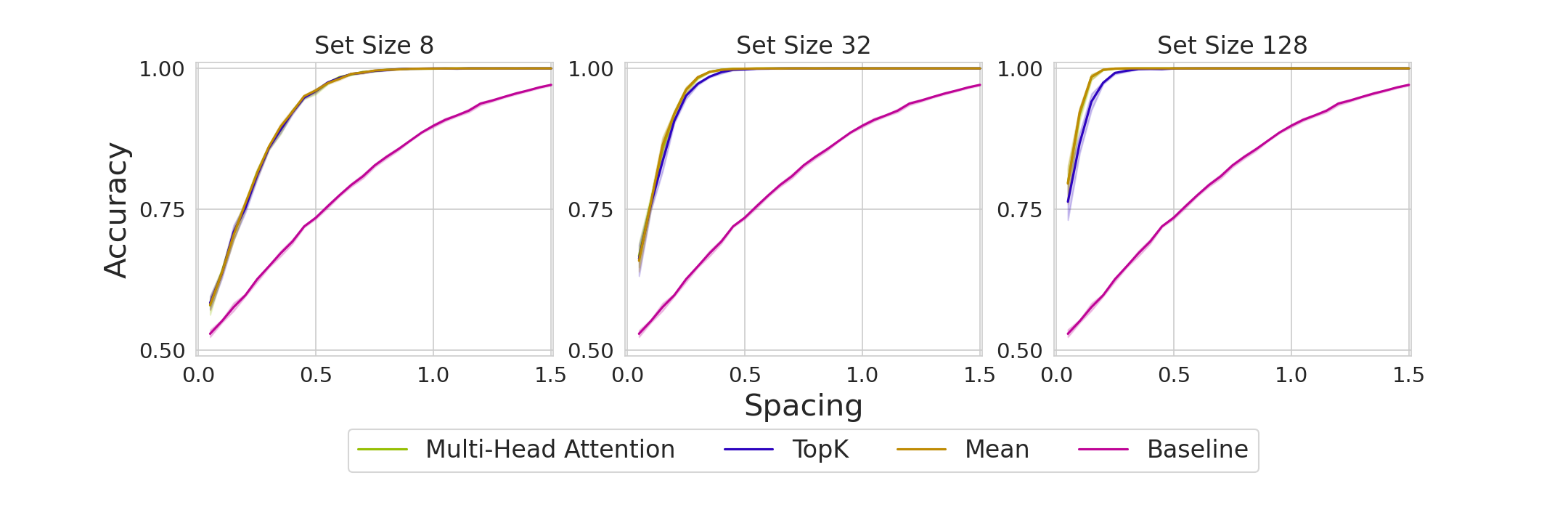
Figure 10: Comparison of different architectural choices for the permutation-invariant network in predicting the data’s originating environment. We consider various distances between environments and different set sizes $n$. As anticipated, the plots illustrate that smaller environment distances make it more challenging to differentiate between them. Moreover, with larger set size $n$, our ability to predict the environment label improves. Notably, the baseline model shows significantly poorer performance compared to the model utilizing contextual information in the form of a set input.

Despite having favorable theoretical properties, plain sum-decompositions can have limited representational capacity in practice [69, 58]. Thus, more expressive permutation-invariant functions can be learned by stacking equivariant transformations with sum-decompositions [69, 7] or by using a self-attention mechanism without positional encodings [33]. In order to re-assess the expressiveness of these methods, we show a comparison of the binary domain classification accuracy based on domain overlap and set size in Figure 10.

2.4 Context-Aware Model

Our model consists of two key components (also illustrated in Figure 1):

• a permutation-invariant network $h_{\boldsymbol{\psi}}$ (“set encoder”) with parameters $\psi$ that maps a set input $\mathbf{S}^{(n)}$ to a summary vector $h_{\boldsymbol{\psi}}(\mathbf{S}^{(n)})$, and

• an inference network $f_{\boldsymbol{\phi}}$ with parameters $\boldsymbol{\phi}$ that maps both the input $\mathbf{X}$ and the summary vector $h_{\boldsymbol{\psi}}(\mathbf{S}^{(n)})$ to a final prediction.

The complete model is denoted as $f_{\boldsymbol{\theta}}(\mathbf{X},\mathbf{S}^{(n)})=f_{\boldsymbol{\phi}}(\mathbf{X},h_{\boldsymbol{\psi}}(\mathbf{S}^{(n)}))$ with parameters $\boldsymbol{\theta}=(\boldsymbol{\psi},\boldsymbol{\phi})$ for short. For a given supervised learning task, we aim to find the minimum to the following optimization problem

$$\boldsymbol{\theta}^{\star}=\operatorname*{arg\,min}_{\boldsymbol{\theta}}\mathbb{E}_{p(\mathbf{X},\mathbf{Y},E)}\left[c(f_{\boldsymbol{\theta}}(\mathbf{X},\mathbf{S}^{(n)}),\mathbf{Y})\right],$$ (3)

where $c$ is a task-specific loss function (e.g., cross-entropy for classification or mean squared error for regression). The algorithmic details for optimizing Equation 3 are detailed in Algorithm 1. For practical reasons, we first apply a feature extractor $g$ and then pass $\{g(\mathbf{X})\mid\mathbf{X}\in\mathbf{S}^{(n)}\}$ as input to the set encoder and $g(\mathbf{X})$ as input to the inference network, building upon the features extracted by $g$. Note, that $g$ can be a pre-trained network, in which case we can treat it as a fixed transformation, or its parameters can be optimized jointly with $\boldsymbol{\theta}$.

Data: Samples from the joint distribution $p(\mathbf{X},\mathbf{Y},E)$

Input : Composite model parameters $\boldsymbol{\theta}$, set size $n$, batch size $m$, loss-function $c$, number of iterations $k$, learning rate schedule $\alpha(k)$

1 for $i=1,\dots,k$ do

2       Sample mini-batch $\mathcal{B}=\{(\mathbf{x}_{1},\boldsymbol{y}_{1},\text{env}_{1}),\dots,(\mathbf{x}_{m},\boldsymbol{y}_{m},\text{env}_{m})\}$ from $p(\mathbf{X},\mathbf{Y},E)$

3       for $j=1,\dots,m$ do

4             Sample set $\mathbf{s}_{j}^{(n)}=\{\mathbf{x}_{1},\dots\mathbf{x}_{n}\}$ from $p(\mathbf{X}\mid E=\text{env}_{j})$

5             Replace $\text{env}_{j}$ with $\mathbf{s}_{j}^{(n)}$ in $\mathcal{B}$

6       end for

7      Update $\boldsymbol{\theta}$ using adaptive mini-batch gradient descent (or any variant):

$$\boldsymbol{\theta}_{k}\leftarrow\boldsymbol{\theta}_{k-1}-\alpha(k)\nabla_{\boldsymbol{\theta}}\left(\sum_{j=1}^{m}c\left(f_{\boldsymbol{\theta}}(\mathbf{x}_{j},\mathbf{s}_{j}^{(n)}),\boldsymbol{y}_{j}\right)\right)$$

8 end for

Output : Trained context-aware model $f_{\boldsymbol{\theta}}$

Algorithm 1 Optimizing Equation 3 for context-aware domain generalization.

2.5 Criteria for Improvement

In the following, we establish criteria under which our method can exploit the distribution shifts between environments and yield improved predictions. In total, we propose three criteria that are necessary to achieve incremental improvement. In Theorem 2.1, we show how these criteria are related to each other. In the formulations below, $I(\mathbf{X};\mathbf{Y})$ denotes the mutual information between random vectors $\mathbf{X}$ and $\mathbf{Y}$ and $I(\mathbf{X};\mathbf{Y}\mid\mathbf{Z})$ denotes the conditional mutual information given a third random vector $\mathbf{Z}$. The symbol $\perp$ (resp. $\not\perp$) between two random vectors $\mathbf{X}$ and $\mathbf{Y}$ is used to express that the random vectors are independent (resp. dependent) or conditionally independent (resp. dependent) given a third random vector $\mathbf{Z}$.

First, we require that given an input $\mathbf{X}$, a further set of i.i.d. inputs $\mathbf{S}^{(n)}$ from the same environment provides incremental information about $\mathbf{Y}$. This is exactly what we need to achieve improved predictive performance, and we can formally define it as our first criterion:

Criterion 2.1.

$\mathbf{S}^{(n)}\not\perp\mathbf{Y}\mid\mathbf{X}$ or equivalently $I(\mathbf{S}^{(n)};\,\mathbf{Y}\mid\mathbf{X})>0$.

The second criterion requires that, given a target input $\mathbf{X}$, a set of further i.i.d. inputs $\mathbf{S}^{(n)}$ from the same environment provides additional information about the origin environment of $\mathbf{X}$.

Criterion 2.2.

$E\not\perp\mathbf{S}^{(n)}\mid\mathbf{X}$ or equivalently $I(E;\,\mathbf{S}^{(n)}\mid\mathbf{X})>0$.

In Figure 1, an instance $\mathbf{X}$ cannot be assigned with complete certainty to an environment. Consequentially, further data provides additional information about the environment. In general, the more data we consider, the better we can predict the originating environment. Crucially, this criterion is not satisfied, if we can recover the origin environment from the singleton input $\mathbf{X}$ alone.

The third criterion requires that the singleton input $\mathbf{X}$ gains information about $\mathbf{Y}$ if we also consider the origin environment $E$ of $\mathbf{X}$.

Criterion 2.3.

$\mathbf{Y}\not\perp E\mid\mathbf{X}$ or equivalently $I(\mathbf{Y};\,E\mid\mathbf{X})>0$.

In Figure 1, this is evidently the case: If we knew the environment from which the data stems, we could improve our prediction of $\mathbf{Y}$. Furthermore, this criterion can serve as a sanity check in case we have an oracle that can identify the origin environment of the data with perfect accuracy.

In what follows, we show that Criterion 2.2 and Criterion 2.3 are necessary conditions for Criterion 2.1. We furthermore prove that if we can extract the environment label fully from $\mathbf{S}^{(n)}$, then Criterion 2.2 and Criterion 2.3 are sufficient conditions for Criterion 2.1. We even generalize this result for the case where the environment label is not inferable with 100% accuracy.

Theorem 2.1.

The following statements hold:

• If $E\perp\mathbf{S}^{(n)}\mid\mathbf{X}$, it follows that $\mathbf{Y}\perp\mathbf{S}^{(n)}\mid\mathbf{X}$. This is equivalent to the implication that if Criterion 2.2 is unattainable, then Criterion 2.1 is also not satisfied.

• If $E\perp\mathbf{Y}\mid\mathbf{X}$, we achieve $\mathbf{Y}\perp\mathbf{S}^{(n)}\mid\mathbf{X}$. This statement corresponds to: Criterion 2.3 is a necessary condition for Criterion 2.1.

• Assume that there exists a deterministic function $g$ with $g(\mathbf{S}^{(n)})=E$, then $\mathbf{Y}\not\perp E\mid\mathbf{X}$ implies $\mathbf{Y}\not\perp\mathbf{S}^{(n)}\mid\mathbf{X}$. This conveys that if we could perfectly infer $E$ from $\mathbf{S}^{(n)}$, then Criterion 2.3 implies Criterion 2.1.

• Assume that there exists a function $g$ and a noise variable $Z$ that elicits the relation $E=g(\mathbf{S}^{(n)})+Z$ and satisfies $\mathbf{S}^{(n)}\perp Z\mid\mathbf{X}$ as well as $\mathbf{S}^{(n)}\perp Z\mid\mathbf{X},Y$. Furthermore, assume that $\mathbf{Y}\not\perp E\mid\mathbf{X}$ and $I(\mathbf{Y};E\mid\mathbf{X})>I(Z;\mathbf{Y}\mid\mathbf{X})$. Then, we achieve $\mathbf{Y}\not\perp\mathbf{S}^{(n)}\mid\mathbf{X}$, recovering Criterion 2.1.

The proof for this theorem and a discussion of its presumptions can be found in Section A.2. Unfortunately, we cannot conclude that $Y\perp\mathbf{S}^{(n)}\mid\mathbf{X}$ follows from Criterion 2.2 and Criterion 2.3 in general. An example where Criterion 2.2 and Criterion 2.3 hold, but Criterion 2.1 is violated, is provided in Section A.1.

2.6 Source Component Shift

Using our approach, we can characterize the kind of distribution shift that allows our criteria to be satifsied. Source component shift refers to the scenario where the data comes from a number of sources (or environments) each with different characteristics [46, Chapter 1.9]. The source component shift can be described by the graphical model in Figure 1, where the environment directly affects both the input $\mathbf{X}$ and the outcome $\mathbf{Y}$. Problems that conform to the graph in Figure 1 have two important implications. First, the input distribution changes whenever the environment changes. Second, the relationship between inputs and outcomes varies with the environment (corresponding to Criterion 2.1). For more details on this kind of distribution shift, we refer the reader to [46, Chapter 1.9]. It is also worth noting that the graph in Figure 1 corresponds to Simpson’s paradox [45, 57], which supplies a proof-of-concept for our approach (see Experiment 1).

2.7 Detection of Novel Environments

During test time, data could either originate from an environment that corresponds to one of the training environments (but its origins are unknown) or from a previously unseen environment. In the following, we explain how we aim to detect the second case that might result in potential failure cases due to fundamental challenges in extrapolation. Following [41], we can define a score $s(h_{\psi}(\mathbf{S}^{(n)}))$ on the summary vector $h_{\boldsymbol{\psi}}(\mathbf{S}^{(n)})$ implicit in our model $f_{\boldsymbol{\theta}}(\mathbf{X},\mathbf{S}^{(n)})$ that aims to predict the target variable $\mathbf{Y}$. As a score function, we consider the distance of $h_{\boldsymbol{\psi}}(\mathbf{S}^{(n)})$ to the $k$-nearest neighbors in the training data in the feature space of the set-encoder. Accordingly, set-representations that elicit a score surpassing a certain threshold are considered to originate from a novel environment. Following the approach in [41], we consider the score distribution and set a threshold to classify a specific percentage, denoted as $q$, of in-distribution samples as originating from a known environment. To establish this threshold, we consider the $q$-th percentile of scores obtained from the validation set. We also compare our novel environment detector with the same score function computed solely from singleton features $g(\mathbf{X})$. These results can be quickly previewed in Table 2.

3 Related Work

3.1 Domain Generalization

The aim of domain generalization (DG) is to train models that generalize well under distribution shifts [39, 74]. The DG setting involves access to data from multiple domains during training exploiting the heterogeneity between domains. In this context, the plethora of algorithms aimed at improving robustness has been divided into three categories [60]: (i) algorithms that enhance the data (e.g., via data augmentation or domain synthesis [56, 68]), (ii) algorithms that adapt the learning algorithm (e.g., self-supervised learning [29, 8]), and (iii) algorithms aiming to find robust representations (e.g., via invariance learning [4, 42]). Our approach explores a different avenue exploiting contextual information about the origin of the data via an adaptive environment embedding.

In contrast to domain adaptation (DA) [61], where samples from the test domain are given during training, in DG no knowledge about the test environment is available during training. As a middle-ground between DA and DG, test-time adaptation (TTA) involves the provision of unlabeled samples during test time, enabling further fine-tuning of the model [35]. TTA can be categorized into test-time domain adaptation, test-time batch adaptation (TTBA), and online test-time adaptation (OTTA) [35].

Among these settings, our work aligns most closely with the TTBA scenario concerning the utilization of environment information. In TTBA a pre-trained model is adapted to one or a few inputs [54, 72, 51]. Each adaptation depends on the mini-batch at hand. Similarly, we consider a mini-batch as a set input to deliver contextual information. However, we do not adapt or fine-tune our model at test time, but rather directly extract context information via the set-encoder. This allows us to identify whether extrapolation is necessary, enabling model misspecification detection [50]. Moreover, since we do not need to fine-tune the model at test time, our approach is considerably more efficient.

Finally, [12] assume a setting where inputs from multiple domains are available, but it is unknown which sample belongs to which environment – even during training time. The authors infer potential domain labels that are used for downstream invariant learning, for example, via Invariant Risk Minimization (IRM) [4]. This method improves on baseline models and enables the application of DG methods in the absence of domain labels. Interestingly, it could be combined with our approach when no environment labels are provided during training, and we leave this as an avenue for future research.

3.2 Learning Permutation-Invariant Representations

Analyzing set-structured data with neural networks has received much theoretical [58, 7, 43] and empirical [69, 33, 70] momentum in recent years. For instance, [70] build on the set transformer architecture [33] and augment the attentive encoder with the capability to learn dynamic templates for attention-based pooling. The resulting “PICASO” blocks include consecutive multi-head attention stacks with skip connections, which update their template(s) depending on previous template(s) and the particular input set (in contrast to global templates). Differently, [13] propose to learn set-specific representations, along with global “prototypes”, using an optimal transport (OT) optimization criterion. The authors also show how to use their criterion for generative and few-shot classification tasks In a somewhat similar vain, [5] investigate a gradient-based optimization method for aggregating set-structured data. Importantly, these methods comprise a pool of algorithms which can be used as the backbone architecture for realizing the set-encoder in our approach.

Model	Symbol	Description	Purpose
Context-aware model (ours)	$f^{\mathbf{Y}\mid\mathbf{X},\mathbf{S}^{(n)}}$	Predicts Y from $\mathbf{X}$ and $\mathbf{S}^{(n)}$	Improve predictions
Baseline model	$f^{\mathbf{Y}\mid\mathbf{X}}$	Predicts Y from $\mathbf{X}$ alone	Verify improvement
Environment-oracle model	$f^{\mathbf{Y}\mid\mathbf{X},E}$	Predicts Y from $\mathbf{X}$ and $E$	Verify Criterion 2.3
Contextual environment model	$f^{E\mid\mathbf{X},\mathbf{S}^{(n)}}$	Predicts $E$ from $\mathbf{X}$ and $\mathbf{S}^{(n)}$	Verify Criterion 2.2
Baseline environment model	$f^{E\mid\mathbf{X}}$	Predicts $E$ from $\mathbf{X}$ alone	Verify Criterion 2.2.

Table 1: The five different model types used to evaluate our approach and verify the theoretical criteria for improvement.

Notably, the methods above impose no probabilistic structure on the set-representations, since the latter are mainly used as deterministic features for downstream tasks. In contrast, probabilistic models attempt to learn a conditional or a marginal distribution over the set-representations. In the Bayesian literature, sets represent finitely exchangeable sequences, embodying the core probabilistic structure of most Bayesian models [44]. In particular, hierarchical or multi-level Bayesian models are used to model the dependencies in nested data, where observations are organized into clusters or levels [64, 21], mirroring the notions of domain or environment in DG. Indeed, hierarchical Bayesian models have been successfully applied in many areas of science, but are typically constrained to linear or generalized linear models (GLMs), prioritizing interpretability over predictive performance.

From a somewhat different Bayesian perspective, IID data represents the starting point for learning invariant summary statistics for parameter estimation or model comparison. The pioneering work on Neural Statisticians [14] tackles the task from a variational perspective, learning global set-representations as part of a generative model. Neural processes [19, 30] comprise a related family of set-based models for prediction and uncertainty quantification in supervised learning tasks, rooted in the spirit of Gaussian processes [48]. Finally, [31] explore a permutation-invariant variational autoencoder (SetVAE) with multiple latent variables trained with a modified ELBO objective. The goal of this and follow-up models [71] is accurate generative performance, less so the learning of compact representations. The theoretical and empirical implications of learning random set-representations falls outside the scope of our current work, but offers a potentially fruitful avenue for future research.

Crucially, none of the above methods pursues the concrete goal of our work, which is improving domain generalization performance through set-based environment representations. For the purpose of achieving this goal, we employ variants of the DeepSet [69] and SetTransformer architectures for our backbone set-encoder throughout all experiments. Interestingly, we observe that our approach is widely robust to the choice of set-encoder architectures in the problems considered.

3.3 OOD Detection and Selective Classification

Detecting unusual inputs that deviate from the examples in the training set has been a long-standing problem of conceptual complexity in machine and statistical learning [3, 67, 52, 23, 66]. Flagging out-of-distribution (OOD) instances involves identifying uncommon data points that might compromise the reliability of machine learning systems [67]. OOD detection is closely related to inference with a reject option (also termed selective classification) [20, 16], which allows classifiers to refrain from making a prediction under ambiguous or novel conditions [25]. The reject option has been extensively studied in statistical and machine learning [24, 18, 22, 62], with early work dating back to the 1950s[11, 10, 24].

More recently, [41] explored the utility of selective classification in DG settings. They investigated various post-hoc scores to define a “competence region” in feature space where a classifier is deemed competent. Post-hoc methods rely on various aspects of pre-trained model outputs, such as the softmax outputs (e.g., [28]), logit outputs (e.g., [26, 36]), or intermediate features (e.g., [2, 53, 59]). In this work, we consider a post-hoc score based on the $k$-nearest neighbors to the training set in feature space similar to [53], which is applicable to both classification and regression settings. Unlike the approach taken in [41], where the focus lies on individual input features, we consider the set summary provided by the set-encoder. Thus, we can identify novel environments even when singleton inputs lack sufficient information.

4 Experiments

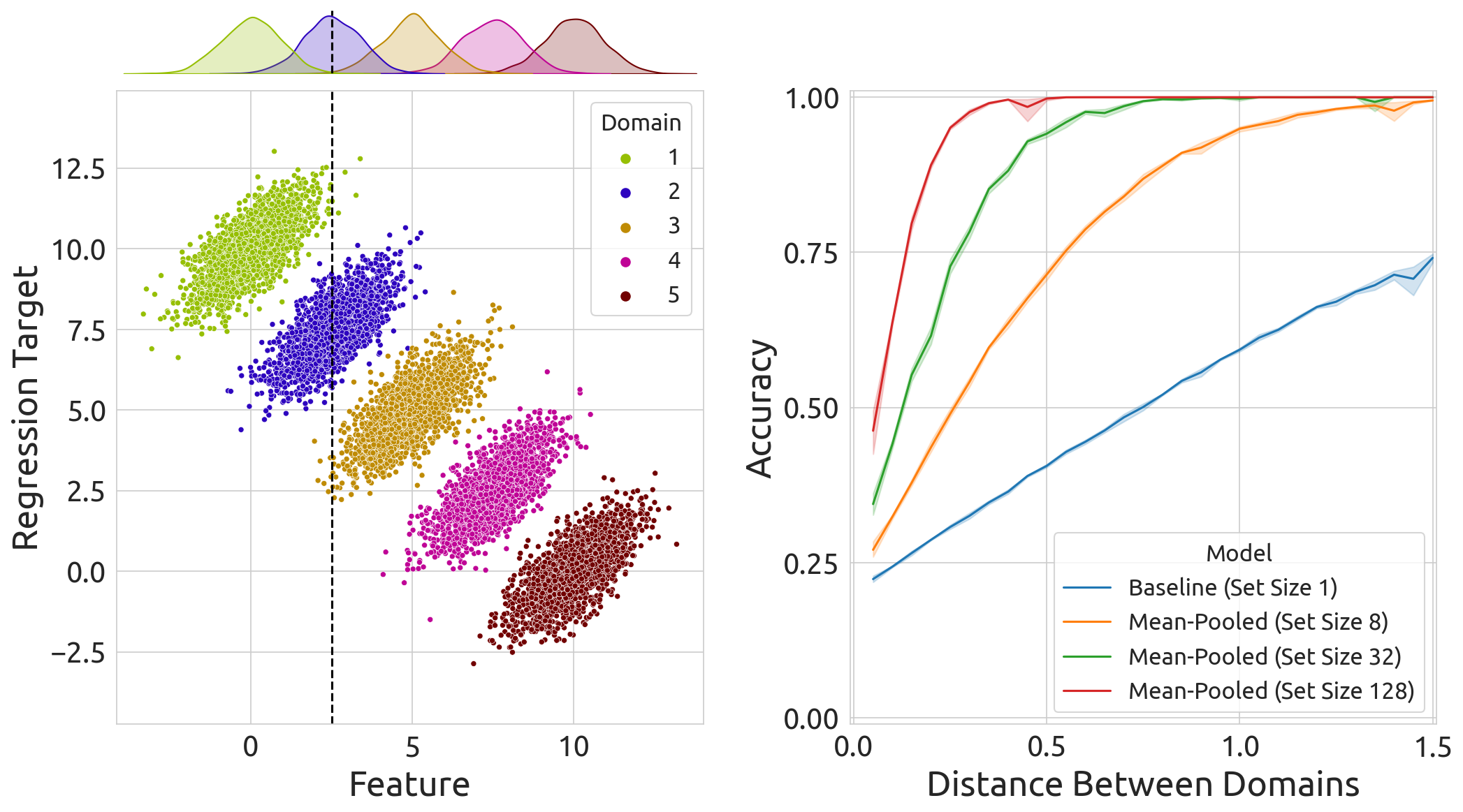
Figure 2: Experiment 1. Left: Toy dataset that conforms to our theoretical criteria. A detailed description can be found in Section C.1. Without environmental information, the marked input at $x=2.5$ could belong to either one of the domains numbered 1, 2, or 3. Marginal distributions of the five environments are shown on top. Right: Comparison of environment classification accuracy for different set sizes.

In the following, we explore various aspects of our approach across three different dimensions. First, we show on two datasets that our model achieves improved performance in the ID as well as the OOD setting compared to a baseline model. Second, we show how novel environments can be detected to select between the most predictive (in the ID setting) and the most robust (in the OOD setting) model. We also show that novel environment detection can be utilized to avoid failure cases. Third, we demonstrate that the necessary criteria (see Section 2.5) can be validated empirically, identifying cases where no benefits of our method can be expected. Experimental details can be found in the Appendix.

4.1 Evaluation Approach

To approximate Criterion 2.1, Criterion 2.2 and Criterion 2.3, we are required to train five distinct models (see Table 1 for an overview). We denote our composite model as $f^{\mathbf{Y}\mid\mathbf{X},\mathbf{S}^{(n)}}$ (see Figure 1) and the baseline model (having no access to the context) as $f^{\mathbf{Y}\mid\mathbf{X}}$. Based on these two models, we can compute the relative improvement achieved by our model relative to a baseline model via

$$\mathcal{R}_{\text{I}}=\frac{\mathcal{L}(f^{\mathbf{Y}\mid\mathbf{X},\mathbf{S}^{(n)}})-\mathcal{L}(f^{\mathbf{Y}\mid\mathbf{X}})}{\mathcal{L}(f^{\mathbf{Y}\mid\mathbf{X}})}.$$ (4)

Here, $\mathcal{L}(f^{\mathbf{Y}\mid\mathbf{X},\mathbf{S}^{(n)}})$ denotes a performance measure for our model and similarly for the baseline model $f^{\mathbf{Y}\mid\mathbf{X}}$. $\mathcal{R}_{\text{I}}>0$ signifies an advantage attained by our approach and therefore the fulfillment of Criterion 2.1. In the regression setting, we consider the negative L2-Loss as the performance measure.

To validate Criterion 2.2, we train a contextual environment model (referred to as $f^{E\mid\mathbf{X},\mathbf{S}^{(n)}}$) utilizing both the set input $\mathbf{S}^{(n)}$ and the target input $\mathbf{X}$ to predict the environment label $E$. Additionally, we train a baseline environment model (denoted as $f^{E\mid\mathbf{X}}$) aimed at predicting $E$ solely from $\mathbf{X}$. We then compute the relative improvement $\mathcal{R}_{\text{II}}$ of the contextual environment predictor relative to the baseline environment predictor. $\mathcal{R}_{\text{II}}>0$ indicates that Criterion 2.2 is satisfied. In our experiments, we choose the set size $n$ such that we achieve approximately 100% accuracy for our contextual environment predictor $f^{E\mid\mathbf{X},\mathbf{S}^{(n)}}$ on ID data.

Similarly, we consider an environment-oracle model $f^{\mathbf{Y}\mid\mathbf{X},E}$ that aims to predict $\mathbf{Y}$ from the singleton input and the environment label $E$. We define the relative improvement $\mathcal{R}_{\text{III}}$ of the environment-oracle model $f^{\mathbf{Y}\mid\mathbf{X},E}$ compared to the baseline method $f^{\mathbf{Y}\mid\mathbf{X}}$. In this case, the relative improvement $\mathcal{R}_{\text{III}}$ is associated with Criterion 2.3.

4.2 Experiment 1: Toy Example

Setup

To set the stage, we consider a dataset that is inspired by [63]. The dataset includes data from five environments, defined by five 2D Gaussian distributions differing only in their locations (i.e., mean vectors). The data-generating process is thus:

$$j \sim\text{Categorical}(p_{1},\dots,p_{J})$$ (5)

$$\mathbf{X}^{(ij)} \sim\mathcal{N}(\boldsymbol{\mu}^{(j)},\mathbf{\Sigma})\quad\text{for}\quad i=1,\dots,I_{j}$$ (6)

This is the classical setting of Simpsons’ paradox, for which a naive linear model fit oblivious to the hierarchical data-generating process will yield results opposite to the true relationship between $X_{1}^{(j)}$ and $X_{2}^{(j)}$ in each environment (cf. Figure 2 and Section C.1 for details).

We designate the first dimension, $X_{1}$, as the input feature, while the second dimension, $Y=X_{2}$, serves as the outcome variable. Importantly, the dataset meets our necessary criteria: We cannot infer the origin environment from a single input alone, as indicated by the overlap between the marginal distributions of $X_{1}$, obtained by projecting the entire sample onto the $x$-axis in Figure 2. Thus, this setting aligns with Criterion 2.2, and, additionally, corresponds to Criterion 2.3, since learning about the environment location $\boldsymbol{\mu}^{(j)}$ should improve prediction.

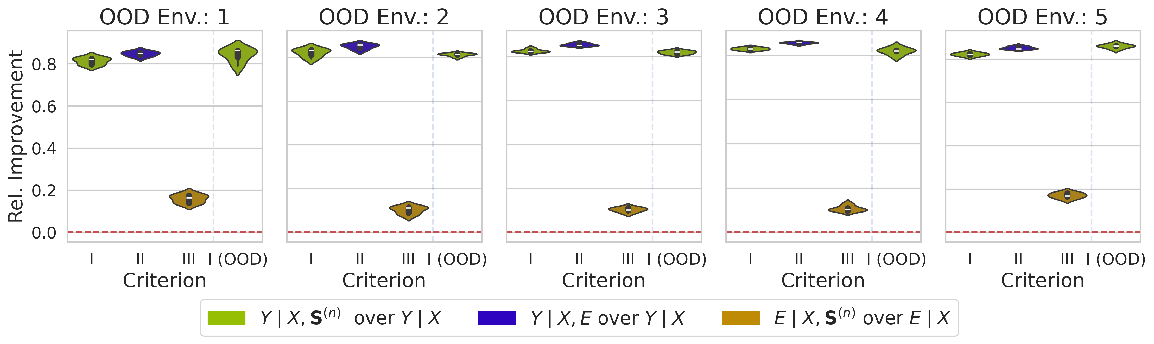
Figure 3: Experiment 1. Relative improvement of set-encoder (shown in I) approach versus baseline model (0 means no improvement is achieved) on toy example. We also show I (OOD) on OOD data. II depicts the relative improvement of the environment-oracle model compared to the baseline model. III demonstrates the relative improvement in predicting the environment when using contextual information compared to the absence of it. Sampling variation arises from using different seeds to partition the ID data into training, test and validation set.

Results

As a first check of Criterion 2.2, we evaluate whether a set input provides additional information about the environment compared to a singleton input. This evaluation involves studying the classification accuracy in distinguishing between the environments. In Figure 2 we observe that the additional set input improves the ability to predict the environment significantly and the more samples we include, the better the prediction. As expected, a decrease in the distance between environments necessitates more samples to differentiate between environments. Interestingly, the particular choice of architecture for the permutation-invariant network does not seem to play a significant role for predicting the environment label well, as demonstrated in Appendix G.

Next, we assess the predictive capabilities of our approach across all possible scenarios of “leave-one-environment-out”. This involves training on all environments except one and treating the excluded environment as a novel OOD scenario. Here, we consider linear models to ensure an optimal inductive bias for the problem (non-linear models achieve similar results, as shown in Section C.3). We can see that Criterion 2.1, Criterion 2.2 and Criterion 2.3 are satisfied in Figure 3. Providing contextual information in the form of a set input increases the performance significantly compared to a baseline model in the ID as well as in the OOD setting (see I and I (OOD) in Figure 3). We also observe a slightly higher relative improvement when the environment label is directly provided (see II) compared to using the output of the set-encoder (see I). This aligns with our expectations, as the set input does not offer more information about the target value than the environment label itself.

Finally, we visualize the predictions of the baseline approach and our set-encoder approach in Figure 4. Our model captures and utilizes the characteristics of each environment for prediction. In contrast, the baseline approach struggles to discern between environments due to the significant overlap between environments, resulting in an inability to deal with environmental differences. Note that we obtained the best results on this problem by considering a class of linear models that aligns with the data-generating process. However, we observe that extrapolation performance drops when the considered models are overly complex and lack a strong inductive bias (see Section C.3).

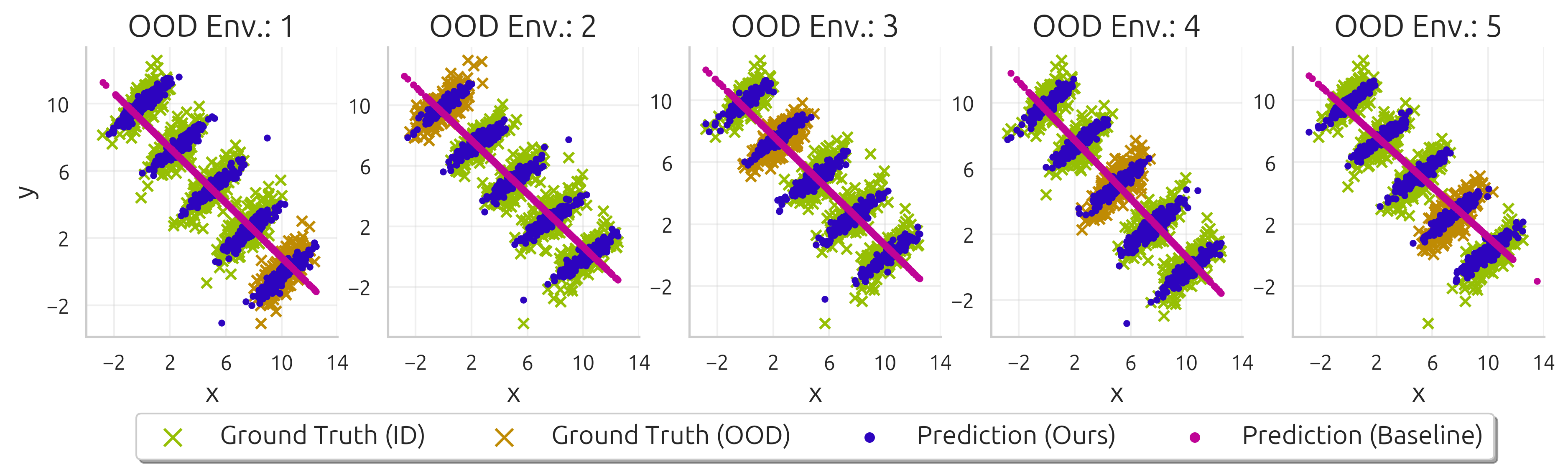
Figure 4: Experiment 1. Predictions performed on the toy dataset illustrated in Figure 2. We show predictions made by both our set-encoder approach and the vanilla model in the ID and OOD settings.

4.3 Experiment 2: ProDAS Example

Setup

We utilize the ProDAS library [40] to generate high-dimensional image data that meets our dataset requirements. The dataset comprises objects of shape square and circle, exhibiting variations in their texture, background color, rotation, and size. Additionally, the background varies in color and texture, resulting in a complex scenario. We consider the task of predicting the object size. Difficulties arise due to the presence of distinct environments with varying characteristics. Specifically, depending on the environment, a constant is added to the observed object size to get the actual target variable that we aim to predict:

$$Y_{\text{gt}}=Y_{\text{observed}}+j\cdot\text{const}_{1}$$ (7)

Here, $j\in\{1,2,3,4\}$ denotes the environment, while $Y_{\text{gt}}$ represents the ground truth (or factual) size, obtained as a sum of the observed size $Y_{\text{observed}}$ (relative to the image frame) and a constant depending on $j$. The background color follows a normal distribution $\mathcal{N}(\boldsymbol{\mu}_{j};\boldsymbol{\Sigma})$ where the mean depends on the environment in the following way: $\boldsymbol{\mu}_{j}=\boldsymbol{\mu}_{0}+j\cdot\text{const}_{2}$. Here we assign a small value to $\text{const}_{2}$ to enforce the background distributions to overlap between different environments. Specifically, this construction implies that the relation between input $\mathbf{X}$ and target $Y$ differs across environments. This corresponds to Criterion 2.3. Notably, inferring the originating environment from a single sample is unattainable due to overlapping background distributions (corresponding to Criterion 2.2). Samples of different environments are shown in Appendix D. This example could be inspired by microscopy data where different microscopes correspond to distinct environments, each exhibiting its own characteristics. During training, we assume to have access to the ground truth value $Y_{\text{gt}}$.

Results

In line with the results from the previous toy example, we can demonstrate a strong relative improvement in the ProDAS dataset, as depicted in Figure 5. All formal criteria are satisfied and a very significant improvement is achieved, both in the ID and the OOD setting, by considering the contextual information from the environment. Details for this experiment can be found in Appendix D.

4.4 Experiment 3: Colored MNIST

Setup

The ColoredMNIST dataset [4] is an extension of the standard MNIST dataset, wherein the number of classes is reduced to two classes (all standard labels $<5$ are assigned to new label 0, and all labels $\geq 5$ are the new label 1). Furthermore, there exists label noise, so only in 75% of all cases, the label can correctly be predicted from the input image. To make things more challenging, the image background can take two colors that are also associated with the image label. In the first environment, the association is 90% and in the second one 80%. Therefore, a baseline model would tend to utilize the background for prediction instead of the actual shape. However, in a third environment, the associations are reversed, so that a model based on the background color would achieve only 10% accuracy – worse than random.

This dataset implies a trade-off between predictive performance in ID domains versus robustness in OOD domains, as discussed in [42]. For instance, an invariant model that relies solely on an object’s shape would be robust to domain shift at the cost of diminished accuracy in the first two environments (75% instead of 80% or 90%). In contrast, a baseline model would achieve greater accuracy in the first domains (80% and 90%), but would fail dramatically in the third domain (only 10%).

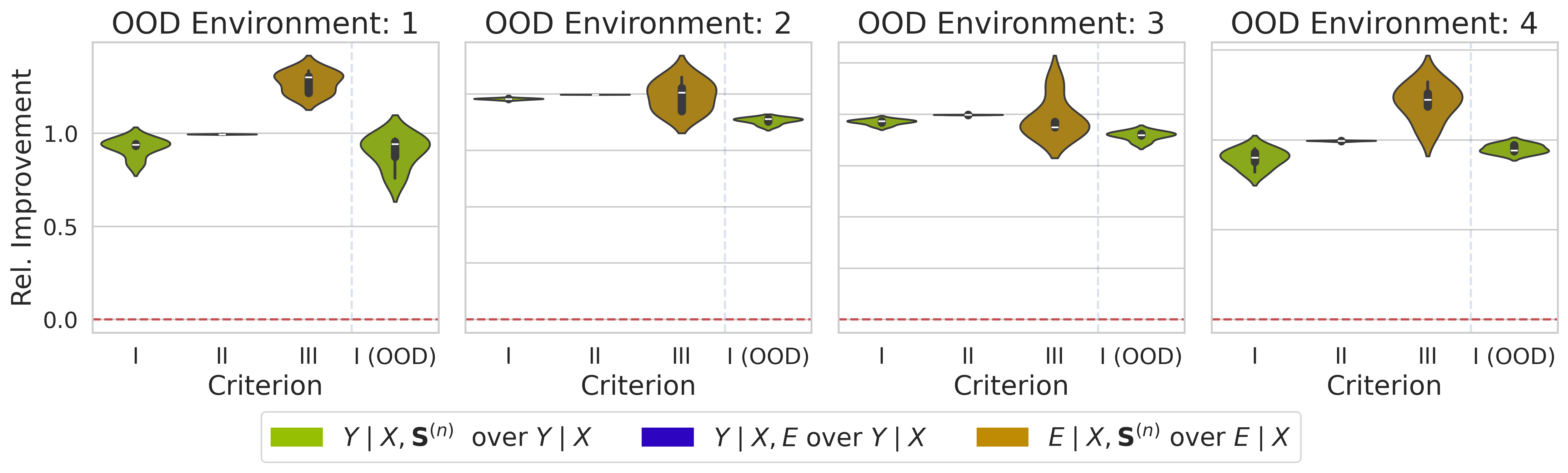
Figure 5: Experiment 2: Relative improvement of set-encoder (shown in I) approach versus baseline model (0 means, no improvement is achieved) on ProDAS dataset. We also show I (OOD) on OOD data. II depicts the relative improvement of the environment-oracle model compared to the baseline model. III demonstrates the relative improvement in predicting the environment when using contextual information compared to the absence of it. Variations arise from using different seeds to partition the ID data into training, test and validation set.

	Accuracy $[\%]$ $\uparrow$
	In-Distribution	Out-of-Distribution
Baseline	$\mathbf{84.6}\pm 0.3$	$10.2\pm 0.3$
Invariant	$72.8\pm 0.9$	$\mathbf{73.1}\pm 0.2$
Selection (Ours)	$\mathbf{84.1}\pm 0.3$	$\mathbf{73.1}\pm 0.2$
Selection (Baseline)	$\mathbf{84.0}\pm 0.3$	$14.0\pm 0.4$
Bayes Optimal Classifier	$\mathbf{85.0}$	$\mathbf{75.0}$

Table 2: Experiment 3. Mean and standard deviation of accuracy percentages across model types and domain settings over 5 runs. The features extracted by our model allow for improved OOD detection compared to the features of the baseline model. Thus, our model can perform a favorable selection between the baseline model in the ID setting and the invariant model in the OOD setting.

Results

Here, we assume the invariant model to be given (see Appendix E for details), but it could also be obtained by invariant learning, e.g. Invariant Risk Minimization [4]. With our novel environment detection approach (see Section 2.7) we can get the best of both worlds, circumventing the inherent trade-off. When identifying the ID setting, we utilize the baseline model that achieves the highest predictiveness within the observed environments. In case we detect the OOD setting, we employ the invariant model. We compare this kind of model selection due to the features $h_{\boldsymbol{\psi}}(\mathbf{S}^{(n)})$ inherent to our model versus the features extracted by the baseline model. The results can be found in Table 2. By utilizing the model selection based on the set-summary $h_{\boldsymbol{\psi}}(\mathbf{S}^{(n)})$, we nearly recover the ID accuracy while maintaining identical performance to the invariant model on OOD data. Evidently, the novel environment detection only works with set summaries. A feature extracted from a single sample does not provide enough information to reliably detect distribution shifts, leading to difficulties in effectively selecting between baseline and invariant model, as demonstrated in Table 2.

4.5 Experiment 4: Violated Criteria

Setup

We consider the PACS dataset [34], training our model on the Cartoons, Sketches, and Paintings environments, and assess its performance in the Art environment during testing. The dataset includes images with labels that we intend to predict. Regarding a second classification task, we delve into the OfficeHome dataset [55]. In line with the PACS dataset, we approach the classification problem, training across three specific environments, and subsequently evaluating a novel one as an out-of-distribution (OOD) scenario.

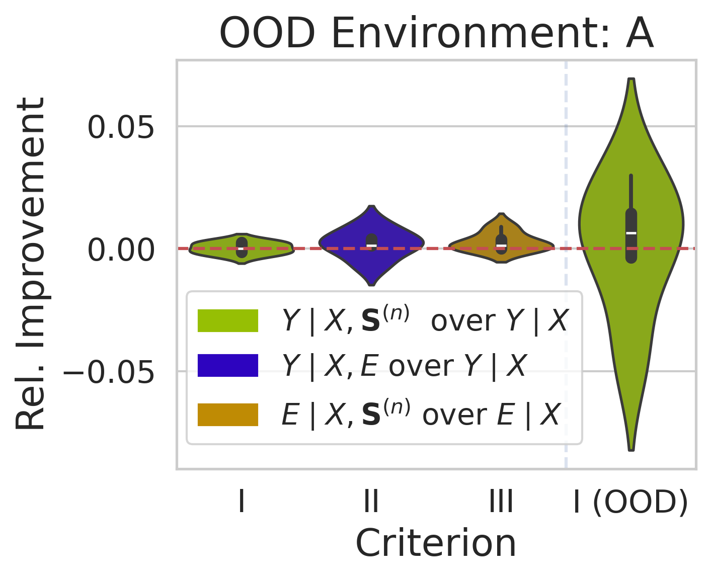
(a) Environment Art in PACS dataset. The environment is almost completely inferable from one input sample (Criterion 2.2 not satisfied). Conclusively our approach does not yield benefits.

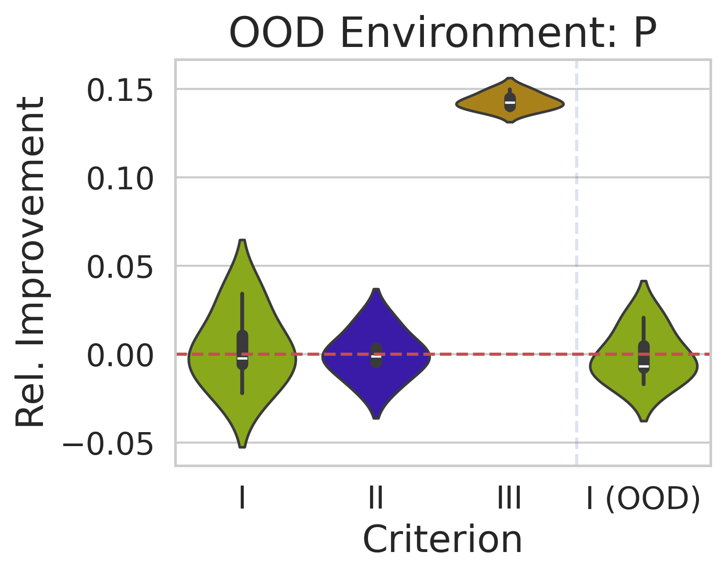
(b) Environment Product in OfficeHome dataset. Although the environment is not inferable from one input sample (Criterion 2.2), the environment information does not yield benefits (Criterion 2.3).

Figure 6: Experiment 4. Examples where at least one of the necessary criteria is not satisfied and our approach cannot possibly yield benefits. For experimental details, see Appendix F.

Results

When the criteria are not met, no benefits can be achieved, even in the ID setting. This has been proven in Theorem 2.1 and we demonstrate it here for two scenarios empirically (see Figure 6). We find that Criterion 2.2 is not satisfied on the PACS dataset: As depicted in 6(b), the contextual environment model $f^{E\mid\mathbf{X},\mathbf{S}^{(n)}}$ does not perform better compared to the baseline environment model $f^{E\mid\mathbf{X}}$. Remarkably, a single example is sufficient to infer the source environment, allowing for a 99.7% accuracy in predicting the correct environment from an individual sample (see Appendix F). Since Criterion 2.2 is not fulfilled, we anticipate Criterion 2.3 also to be wrong. This is indeed the case as 6(b) depicts. Since the criteria are not met, we do not achieve any benefit over the baseline model, neither in the ID nor in the OOD setting, as demonstrated in 6(b).

On the OfficeHome dataset we find that Criterion 2.2 is not satisfied, while Criterion 2.3 is. Results are depicted in 6(b). We observe that the set input offers benefits for predicting the data originating environment corresponding to Criterion 2.3. However, even when providing the target classifier with the environment label (environment-oracle model), we do not achieve an improvement over the baseline model suggesting that Criterion 2.2 is not satisfied. As expected and depicted in 6(b), our method does not yield benefits compared to the baseline model.

4.6 Experiment 5: Failure Case Detection

Setup

Besides unfulfilled criteria, another reason why our approach might fail to reap benefits or degrade in performance is when the distribution shift requires extrapolation. This might be unattainable by the model. We demonstrate, using the BikeSharing dataset [17], that in cases where different seasons like summer or winter represent distinct environments, extrapolation might be necessary. For this dataset we consider the task of predicting the number of bikes rented across the day based on weather data. Details about the dataset and pre-processing steps can be found in Appendix H. We explore four scenarios, each entailing training on all seasons except one. We aim to assess the abilities of our model compared to a baseline model in detecting novel environments.

Results

In Table 3 we demonstrate that our approach is slightly superior compared to the baseline model in the ID settings. However, both the baseline and our approach experience performance degradation in the novel environments. To detect the novel environment (and consequentially potential failure cases), we compute the score as suggested in Section 2.7 and evaluate how well it distinguishes between ID versus OOD environment. We designate an independent ID test set and use the environment excluded during training (e.g., summer or winter) as the OOD set for evaluation. The area under the ROC-curve (AUROC) in Table 3 demonstrates that the score based on the summary vector provided by the permutation invariant network allows for a perfect novel environment detection whereas the standard approach fails in detecting the novel environment.

Table 3: Experiment 5. Performance comparison between our model and the baseline, broken down by target domain. We compare the performance in the ID and OOD setting (MSE), as well as their capability to detect a novel environment (AUROC). Both models fail in the OOD setting, but our model can detect with strong certainty when this is the case. We present the mean and standard deviation derived from 5 runs using different seeds for partitioning into training, validation, and test sets.

5 Conclusions

In this work, we introduce a novel approach enabling the extraction and utilization of contextual information from set inputs within a Domain Generalization (DG) setting. The set inputs originate from the same environment as the sample for which a prediction is required and are summarized into a vector via a permutation-invariant network. We formulate criteria that are necessary for our approach to yield benefits and are easy to verify. Empirically, we demonstrate that we can verify these criteria, which enables us to identify cases where our approach does not yield benefits. We showcase the merits of our approach on several datasets. Additionally, we demonstrate that novel environments can be detected, allowing for the identification of potential failure cases.

In our current framing, we have not yet employed regularization techniques, such as enforcing the set vector to contain all information about the environment in our composite model in Figure 1. In general, investigating inductive biases for the composite network architecture is an interesting future research avenue. Finally, even though we focused our experiments in standard supervised learning settings, our method could also be employed in other realms, such as domain disentanglement, data generation, or in combination with other DG methods. Thus, extending our method to different settings represents another exciting research direction.

Acknowledgments

JM and UK were supported by Informatics for Life funded by the Klaus Tschira Foundation. We thank Florian Fallenbüchel, Felix Draxler, and Armand Rousselot for their support and fruitful discussions.

Appendix A Theory

A.1 Insufficiency of Criteria 2 and 3 for Criteria 1

Criterion 2.2 and Criterion 2.3 are not sufficient to imply Criterion 2.1. This can be seen in an example with three environments $j\in\{1,2,3\}$. Assume the first two have completely identical input distributions. We presume that both input distributions adhere to a uniform distribution $\mathcal{U}[a,b]$. Furthermore, we assume that the third input distribution also follows a uniform distribution that is slightly shifted, i.e. $\mathcal{U}[a+\frac{a+b}{2},b+\frac{a+b}{2}]$. Due to the overlap between the third and the first two environments, a set input provides additional information about $E$ compared to a single sample $X$, verifying Criterion 2.2.

Regarding the mechanism relating inputs to outputs, we assume that on $[a,\frac{a+b}{2}]$ the relation between input $X$ and output $Y$ differs, e.g., two constant functions with distinct values. We further assume that on $(\frac{a+b}{2},b+\frac{a+b}{2}]$ the relation between input $X$ and output $Y$ does not vary with the environment, e.g., is constant. This aligns with Criterion 2.3: if we know the environment, we can improve the prediction, specifically on $[a,\frac{a+b}{2}]$.

However, Criterion 2.1 is not satisfiable. The set input allows us to distinguish environment 3 (i.e. the one with support $\mathcal{U}[a+\frac{a+b}{2},b+\frac{a+b}{2}]$) from the other ones. Yet, we cannot distinguish between environment 1 and environment 2. Since the relation between $X$ and output $Y$ differs only in the supports of environment 1 and environment 2 (specifically, it differs in $\mathcal{U}[a,\frac{a+b}{2}]$), the set input cannot provide additional information about the output $Y$ compared to the single input $X$, i.e. it holds $Y\perp\mathbf{S}^{(n)}\mid X$,

A.2 Proof of Theorem

In the following, we give proofs of Theorem 2.1 (a) - (d).

Proof.

For the upcoming proofs, we extensively employ the chain rule of mutual information:

$$I(\mathbf{Y};Z,\mathbf{X})=I(\mathbf{Y};Z\mid\mathbf{X})+I(\mathbf{Y};\mathbf{X})$$ (8)

Additionally, we have the inequalities $I(\mathbf{Y};\mathbf{S}^{(n)}\mid\mathbf{X})\leq I(\mathbf{Y};E\mid\mathbf{X})$ and $I(\mathbf{S}^{(n)};\mathbf{Y}\mid\mathbf{X})\leq I(E;\mathbf{Y}\mid\mathbf{X})$ that follow from the data processing inequality and how $\mathbf{S}^{(n)}$ relates to the other variables (see Figure 1).

For (b): We easily achieve

$$I(Y;\mathbf{S}^{(n)},\mathbf{X}) =I(\mathbf{Y};\mathbf{S}^{(n)}\mid\mathbf{X})+I(\mathbf{Y};\mathbf{X})$$ (9)

$$\leq I(\mathbf{Y};E\mid\mathbf{X})+I(\mathbf{Y};\mathbf{X})$$ (10)

$$=I(\mathbf{Y};\mathbf{X})$$ (11)

Therefore, we have

$$0\leq I(\mathbf{Y};\mathbf{S}^{(n)}\mid\mathbf{X})=I(\mathbf{Y};\mathbf{S}^{(n)},\mathbf{X})-I(\mathbf{X};\mathbf{Y})\leq 0$$ (12)

which proves (a).

For (a): We can write

$$I(\mathbf{S}^{(n)};\mathbf{Y},\mathbf{X}) =I(\mathbf{S}^{(n)};\mathbf{Y}\mid\mathbf{X})+I(\mathbf{S}^{(n)};\mathbf{X})$$ (13)

$$\leq I(\mathbf{S}^{(n)};E\mid\mathbf{X})+I(\mathbf{S}^{(n)};\mathbf{X})$$ (14)

$$=I(\mathbf{S}^{(n)};\mathbf{X})$$ (15)

and therefore

$$0\leq I(\mathbf{Y};\mathbf{S}^{(n)}\mid\mathbf{X})=I(\mathbf{S}^{(n)};\mathbf{Y},\mathbf{X})-I(\mathbf{X},\mathbf{S}^{(n)})\leq 0$$ (16)

and conclusively $\mathbf{Y}\perp\mathbf{S}^{(n)}\mid\mathbf{X}$.

For (c) is easily seen that $0<I(\mathbf{Y};E\mid\mathbf{X})=I(\mathbf{Y};g(\mathbf{S}^{(n)})\mid\mathbf{X})\leq I(\mathbf{Y};\mathbf{S}^{(n)}\mid\mathbf{X})$ and therefore (c) holds true.

For (d), we also employ the entropy $h(\mathbf{X})$ as well as the conditional entropy $h(\mathbf{X}\mid\mathbf{Y})$. We first establish that $I(A+B;C)\leq I(A;C)+I(B;C)$ for any RVs $A,B,C$ with $A\perp B$ and $A\perp B\mid C$:

$$I(A+B;C) =h(A+B)-h(A+B\mid C)$$

$$\overset{(\star)}{=}\left(h(A)+h(B)-h(A\mid A+B)\right)-\left(h(A\mid C)+h(B\mid C)-h(A\mid A+B,C)\right)$$

$$=I(A;C)+I(B;C)-h(A\mid A+B)+h(A\mid A+B,C)$$

$$\overset{(\star\star)}{\leq}I(A;C)+I(B;C)$$ (17)

$(\star)$ follows with the chain rule for entropy

$$h(A,A+B) =h(A)+h(A+B\mid A)$$ (18)

$$=h(A)+h(B\mid A)\overset{A\perp B}{=}h(A)+h(B)$$ (19)

$$=h(A+B)+h(A\mid A+B)$$ (20)

which implies $h(A+B)=h(A)+h(B)-h(A\mid A+B)$ and equally when conditioning on $C$.

$(\star\star)$ follows since $h(A\mid A+B,C)\leq h(A\mid A+B)$.

Section A.2 can be extended to the conditional mutual information if $A\perp B\mid D$ and $A\perp B\mid D,C$:

$$I(A+B;C\mid D)\leq I(A;C\mid D)+I(B;C\mid D)$$ (21)

Since $\mathbf{S}^{(n)}\perp Z\mid\mathbf{X}$ and $\mathbf{S}^{(n)}\perp Z\mid\mathbf{X},Y$, we achieve

$$0<I(\mathbf{Y};E\mid\mathbf{X}) =I(Y;g(\mathbf{S}^{(n)})+Z\mid\mathbf{X})$$ (22)

$$\leq I(\mathbf{Y};g(\mathbf{S}^{(n)})\mid\mathbf{X})+I(\mathbf{Y};Z\mid\mathbf{X})$$ (23)

$$\leq I(\mathbf{Y};\mathbf{S}^{(n)}\mid\mathbf{X})+I(\mathbf{Y};Z\mid\mathbf{X})$$ (24)

and therefore

$$0<I(\mathbf{Y};E\mid\mathbf{X})-I(\mathbf{Y};Z\mid\mathbf{X})\leq I(\mathbf{Y};\mathbf{S}^{(n)}\mid\mathbf{X})$$ (25)

which concludes the proof. ∎

In the following, we discuss the assumptions in (c) and (d). In our experiments, we observed that in most datasets a relatively small sample size suffices to infer the environment label with approximately 100% accuracy (see Table 5). Therefore, the assumption that there exists a function $g(\mathbf{S}^{(n)})=E$ seems justified if $n$ is sufficiently large. To generalize the assumption where the environment label is not fully inferable, we have to make assumptions. For one, we require $\mathbf{S}^{(n)}\mid Z\mid\mathbf{X}$. This can be interpreted as “increasing the set size does not improve the prediction of $E$”. Also $\mathbf{S}^{(n)}\perp Z\mid\mathbf{X},Y$ can be interpreted similarly: increasing the set size and considering the ground truth label/value does not enhance the predictability of $E$. Both assumptions should hold approximately if $n$ is large enough. With the assumption $I(\mathbf{Y};E\mid\mathbf{X})>I(Z;\perp\mathbf{Y}\mid\mathbf{X})$ we assume that the noise $Z$ is less predictive of $Y$ compared to $E$ if $\mathbf{X}$ is given. This can be roughly interpreted as the noise does not prove useful for predicting $Y$ from $\mathbf{X}$ compared to the ground truth environment label.

Appendix B Experiments: General Remarks

We define the relative improvements $\mathcal{R}_{\text{II}}$ and $\mathcal{R}_{\text{III}}$ as

$$\mathcal{R}_{\text{II}}=\frac{\mathcal{L}(f^{E\mid\mathbf{X},\mathbf{S}^{(n)}})-\mathcal{L}(f^{E\mid\mathbf{X}})}{\mathcal{L}(f^{E\mid\mathbf{X},\mathbf{S}^{(n)}})}$$ (26)

and

$$\mathcal{R}_{\text{III}}=\frac{\mathcal{L}(f^{\mathbf{Y}\mid\mathbf{X},E})-\mathcal{L}(f^{\mathbf{Y}\mid\mathbf{X}})}{\mathcal{L}(f^{\mathbf{Y}\mid\mathbf{X},E})}$$ (27)

$\mathcal{R}_{\text{II}}$ signifies the relative performance gain in predicting the environment when the set input is given compared to the solitude input. In contrast, $\mathcal{R}_{\text{III}}$ denotes the relative performance improvement of the environment-oracle model compared to the baseline model.

Due to the large amount of settings, we did only little hyper-parameter optimization (we looked into batch size, learning rate, and network size). For a given dataset we optimized only on one scenario where an environment is left out during training. The found hyper-parameters were then applied on all other scenarios. To ensure that the baseline model is comparable to ours, we ensure that the inference network (and feature extractor) in Figure 1 have a comparable number of parameters as the baseline model. In all cases, the set-encoder is kept simple and its hyper-parameters are selected for optimal performance of the contextual environment predictor $f^{E\mid\mathbf{X},\mathbf{S}^{(n)}}$. For an overview, see Table 5. Throughout all experiments, we employ a mean-pooling operation.

We show the accuracies of classifying the environment of the contextual-environment model $f^{E\mid\mathbf{X},\mathbf{S}^{(n)}}$ and the baseline environment model $f^{E\mid\mathbf{X}}$ in Table 5. Here we only consider the datasets where we performed a full evaluation of all criteria.

Appendix C Experiment 1: Details

C.1 Data Generation

Simpson’s Paradox [45, 57] describes a statistical phenomenon wherein several groups of data exhibit a trend, which reverses when the groups are combined. There are several famous real-world examples of Simpson’s Paradox, such as a study examining a gender bias in the admission process of UC Berkeley [6] or an evaluation of the efficacy of different treatments for kidney stones [9].

In order to replicate this, we create a dataset as a mixture of 2D multivariate normal distributions, with the intent of using the first dimension as a feature, and the second as a regression target. Unless otherwise specified, we generate the data by taking an equal number of samples from each mixture component, defining the environment as a one-hot vector over the mixture components.

The mixture components are chosen to lie on a trend line that is opposite to the trend within each mixture. We achieve this by using a negative global trend, and choosing the covariance matrix of each mixture as a scaled and rotated identity matrix with opposite trend.

Setting	Value	Controls
n_domains	$5$	number of mixture components
n_samples	$10000$	number of samples per mixture component
spacing	$2.0$	spacing between means of the mixture components
noise	$0.25$	overall noise level
noise_ratio	$6.0$	ratio of the primary to secondary noise axis
rotation_range	$(45.0,45.0)$	min (leftmost) and max (rightmost) mixture rotation angle

Table 4: Default Settings for the Simpson’s Paradox Dataset. Samples from the dataset constructed with these settings can be seen in Figure 2

The YouTube channel minutephysics also published a short descriptive video on this phenomenon in 2017 [38].

C.2 Training Details

We consider five distinct settings, where in each setting, one domain is left out during training, and considered for evaluation as a novel environment. To gauge the uncertainty stemming from data sampling, we also consider five dataset seeds for partitioning into training, validation, and test sets. For each dataset seed and model, we consider the results due to the best performance on the validation set.

We enforced that our approach and the baseline model have a similar amount of parameters for the feature extractor and final inference model. We conducted minimal hyperparameter tuning (focusing on parameters such as the learning rate schedule, batch size, and the number of parameters), and this was performed solely within one “leave-one-environment-out” setting. In total, we trained the five models outlined in Table 1 using five distinct dataset seeds. Consequently, a total of $5\cdot 5\cdot 5=125$ models were trained. In all cases, the set-encoder is kept simple and its hyper-parameters are selected for optimal performance of the contextual environment predictor $f^{E\mid\mathbf{X},\mathbf{S}^{(n)}}$. We choose the mean as the pooling operation.

C.3 Non-Linear Models

In the experiments in Section 4.2, we considered linear models for our model and the baseline. In the following, we show results for the non-linear model class in Figure 7. We compare predictions of a baseline model and our model on all environments in Figure 8. We see that the extrapolation task fails in some cases as in environment 1. This is due to the mismatch of the considered model class and ground truth model.

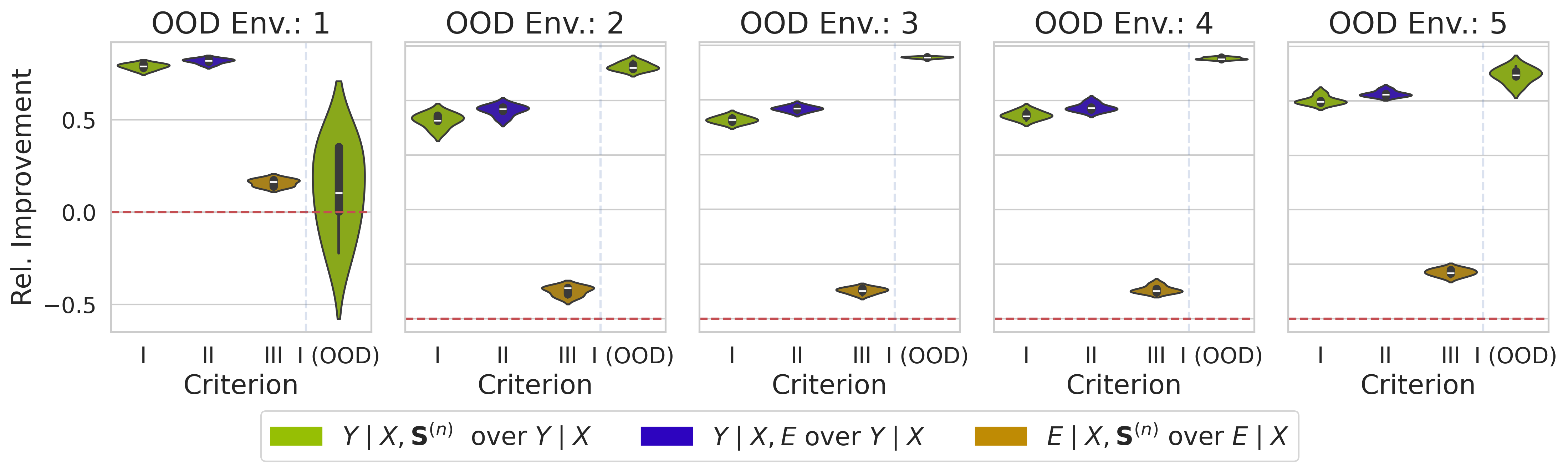
Figure 7: Experiment 1. Verification of criteria. In I we depict the relative improvement of our approach versus a baseline model. We also show I (OOD) on OOD data. In II we show the relative improvement of the oracle model compared to the baseline. In III we compare the relative improvement of the contextual environment model with respect to the baseline environment model.

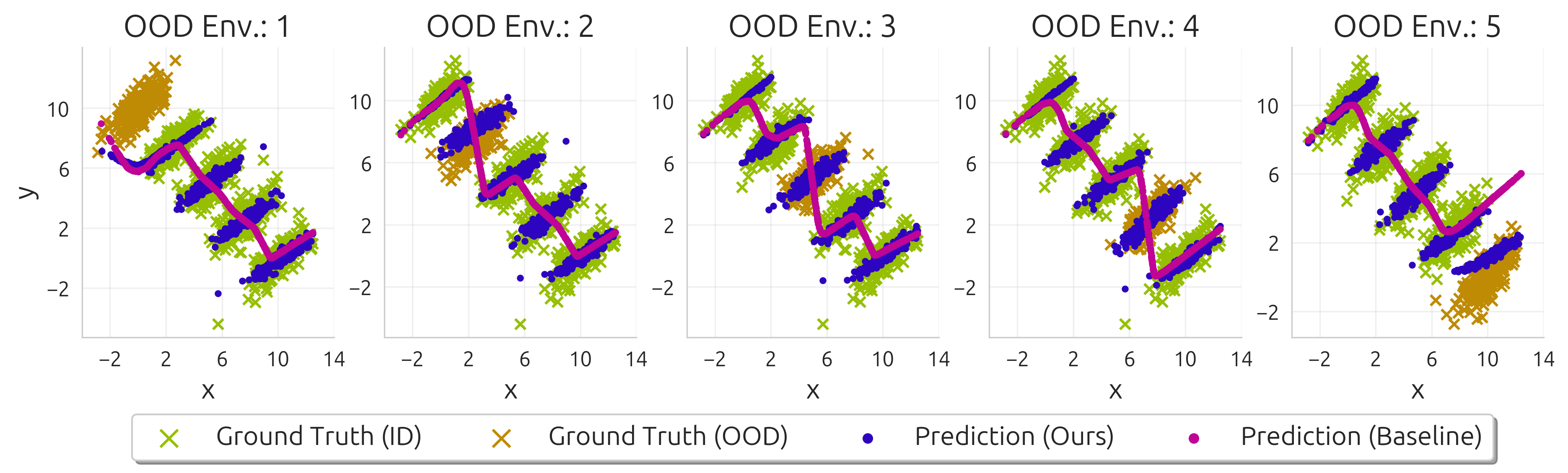
Figure 8: Experiment 1. Models are trained on all environments except the OOD environment. “Extrapolation”, i.e. when environment 1 or 5 is OOD, is a particularly hard task in this setting. The set-based model shows slightly better extrapolation capabilities. Generally, our model exhibits adaptability to diverse environments, addressing a limitation present in the baseline model.

Appendix D Experiment 2: Details

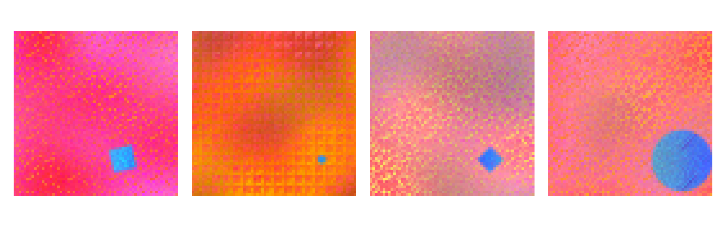
(a) Environment 1

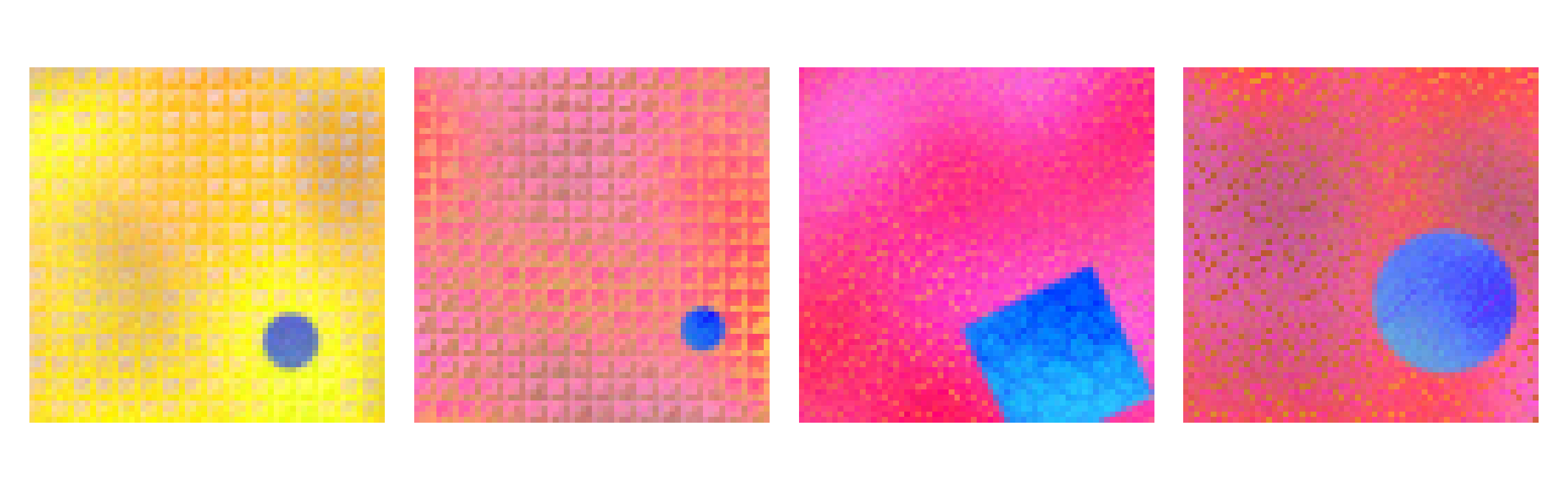
(b) Environment 2

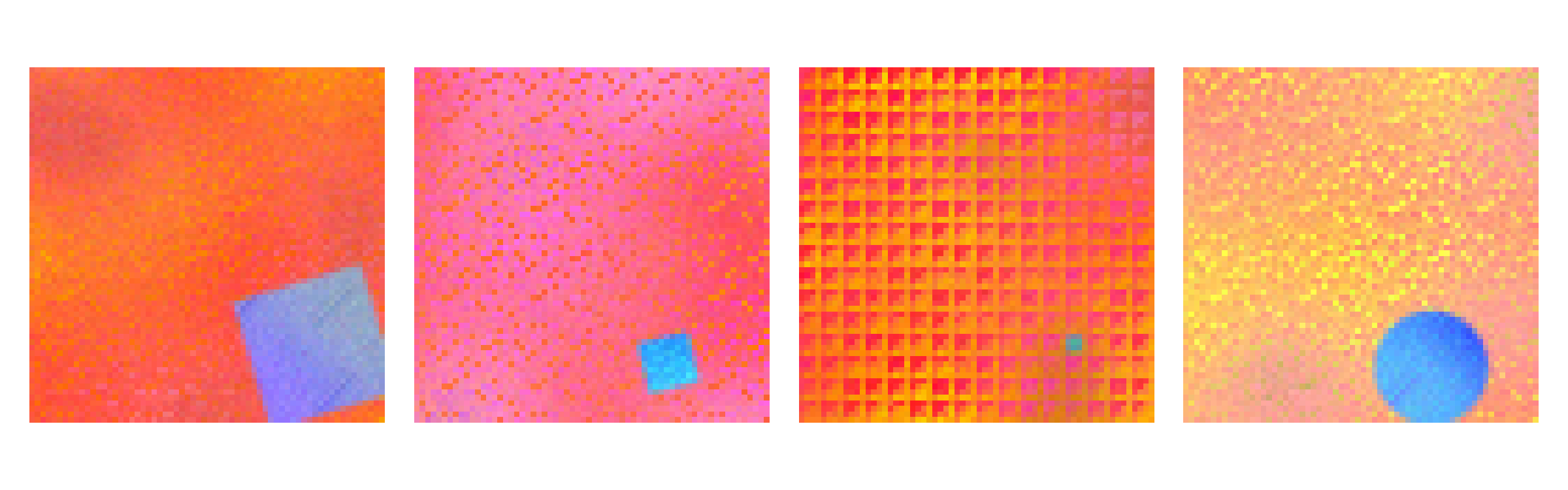
(c) Environment 3

(d) Environment 4

Figure 9: Experiment 2. We generate four distinct domains synthetically. Notably, the background color within each domain follows a normal distribution. However, there are variations in the means across these domains Note that there is a huge overlap between the environments.

Data samples from different environments are depicted in Figure 9. The process of how inputs relate to outputs is described in Section 4.3.

During training, we employ a convolutional network to extract features $g(\mathbf{X})$. These features are passed to the inference network and the set-encoder. The feature extractor is then jointly trained with the inference network and set-encoder. We ensured that the feature extractor plus inference network and the baseline model have a comparable amount of parameters. The set-encoder is kept simple and its hyper-parameters are selected for optimal performance of the contextual environment predictor $f^{E\mid\mathbf{X},\mathbf{S}^{(n)}}$. As a pooling operation we choose the mean-pooling.

Appendix E Experiment 3: Details

To select between the baseline model and the invariant model, we are required to distinguish between ID and OOD data. Therefore, we follow the approach proposed in Section 2.7. We consider the $k$-nearest neighbors of the training set to compute the score $s_{\boldsymbol{\psi}}$ where $k=5$. Since we compare the scores elicited by features of the baseline model with the scores elicited by the features extracted by the set-encoder, we restricted both architectures to have the same feature dimension. To establish a threshold for distinguishing between ID and OOD samples, we designate samples with scores below the 95% quantile of the validation set as ID and those above as OOD (see Section 2.7 for details).

In total, we explore five dataset seeds to partition into training, validation, and test sets. To train an invariant model, we considered the same split in training, validation, and test set where the background color has no association with the label. Therefore the invariant model learns to ignore the background color and only utilize the shape for prediction. To learn effectively about the environment, we considered a large set input, namely 1024 samples in $\mathbf{S}^{(n)}$. We employed a simple set-encoder incorporating a mean pooling operation.

Appendix F Experiment 4 and 5: Details

For the BikeSharing dataset we consider a simple feed-forward neural network in all models. For the PACS as well as the OfficeHome dataset we consider features $g(\mathbf{X})$ that are kept fixed and not optimized. Here, we employ the Clip features proposed in [47]. The inference model, baseline model, and set-encoder are kept simple and employ only linear layers followed by ReLU activation functions. Given that Clip features considerably simplify the task, we performed a minimal hyper-parameter search and ensured that the inference model had a similar number of parameters as the baseline model. In all cases, the set-encoder is kept simple and its hyper-parameters are selected for optimal performance of the contextual environment predictor $f^{E\mid\mathbf{X},\mathbf{S}^{(n)}}$.

Dataset / Set Size	Simpson / $32$
Domain	1	2	3	4	5
$f^{E\mid\mathbf{X}}$	$86.3\pm 1.3$	$90.8\pm 1.3$	$90.7\pm 0.8$	$90.4\pm 0.9$	$85.5\pm 0.8$
$f^{E\mid\mathbf{X},\mathbf{S}^{(n)}}$	$\mathbf{100.0}\pm 0.0$	$\mathbf{100.0}\pm 0.0$	$\mathbf{100.0}\pm 0.0$	$\mathbf{100.0}\pm 0.0$	$\mathbf{100.0}\pm 0.0$

Dataset / Set Size	ProDAS / $128$				OfficeHome / $4$	PACS / $4$
Domain	1	2	3	4	Product	Art
$f^{E\mid\mathbf{X}}$	$43.8\pm 1.1$	$50.0\pm 1.3$	$49.9\pm 2.3$	$44.4\pm 1.0$	$86.16\pm 0.33$	$\mathbf{99.72}\pm 0.33$
$f^{E\mid\mathbf{X},\mathbf{S}^{(n)}}$	$\mathbf{99.6}\pm 0.6$	$\mathbf{99.5}\pm 1.0$	$\mathbf{98.7}\pm 1.6$	$\mathbf{98.0}\pm 3.2$	$\mathbf{98.49}\pm 0.24$	$\mathbf{100.0}\pm 0.0$

Table 5: Environment classification accuracy for different models and datasets, broken down by domain. As in Table 3, the uncertainty (mean and standard deviation) is computed over multiple seeds for dataset splits. In all cases, the set-based model outperforms the baseline.

In all cases, the set-encoder is kept simple and its hyper-parameters are selected for optimal performance of the contextual environment predictor $f^{E\mid\mathbf{X},\mathbf{S}^{(n)}}$.

Appendix G Comparison of Permutation-Invariant Architectures

As a pilot experiment, we estimate the contextual information contained in a set input by evaluating the binary classification accuracy of a set-based model compared to a baseline model with singleton sample input.

Importantly, we postulate that for stronger domain overlap, the contextual information contained within the single sample decreases significantly, while the contextual information within the set decreases only weakly, depending on the set size. Domains that do not overlap exactly will remain distinguishable, so long as the set size is large enough.

Therefore, we construct the toy dataset as described in Section C.1, but use the setting n_domains = 2 and vary the distance between environments for each experiment.

We train each architecture on this dataset for $20$ epochs, using $5$ different seeds. We evaluate a total of $30$ domain spacings, linearly distributed between $0.05$ and $1.5$ (both inclusive). Since we evaluate a baseline model, plus 3 set-based models at 3 different set sizes, this brings us to a total of $30\cdot 20\cdot 5\cdot(1+3\cdot 3)=30000$ model epochs. We choose the batch size at $128$ fixed.

Each architecture consists of a linear projection into a $64$-dimensional feature space, followed by a fully connected network with $3$ hidden layers, each containing $64$ neurons and a ReLU [1] activation. For the set-based methods, this is followed by the respective pooling. We choose $8$ heads for the attention-based model.

Finally, the output is linearly projected back into the $2$-dimensional logit space, where the loss is computed via cross-entropy [73].

For methods that support a non-unit output set size, we choose the output set size as $4$. The output set is mean-pooled prior to projection into the logit space.

Appendix H Bike Sharing Dataset

This dataset, taken from the UCI machine learning repository[17], consists of over $17000$ hourly and daily counts of bike rentals between 2011 and 2012 within the Capital bikeshare system.

Each dataset entry contains information about the season, time, and weather at the time of rental. Casual renters are also distinguished from registered ones.

Similar to [49], we only consider the hourly rental data. We drop information about the concrete date and information about casual versus registered renters. We choose the season variable (spring, summer, fall, winter) as the environment and the bike rental count as the regression target. Since we deal with count data, we also apply square root transformation on the target similar to [49].

References

- [1] Abien Fred Agarap. Deep learning using rectified linear units (relu), 2019.
- [2] Charu C Aggarwal and Charu C Aggarwal. An introduction to outlier analysis. Springer, 2017.
- [3] Charu C Aggarwal and Philip S Yu. Outlier detection for high dimensional data. In Proceedings of the 2001 ACM SIGMOD international conference on Management of data, pages 37–46, 2001.
- [4] Martin Arjovsky, Léon Bottou, Ishaan Gulrajani, and David Lopez-Paz. Invariant risk minimization. arXiv preprint arXiv:1907.02893, 2019.
- [5] Sergey Bartunov, Fabian B Fuchs, and Timothy P Lillicrap. Equilibrium aggregation: encoding sets via optimization. In Uncertainty in Artificial Intelligence, pages 139–149. PMLR, 2022.
- [6] P. J. Bickel, E. A. Hammel, and J. W. O’Connell. Sex bias in graduate admissions: Data from berkeley: Measuring bias is harder than is usually assumed, and the evidence is sometimes contrary to expectation. Science, 187(4175):398–404, February 1975.
- [7] Benjamin Bloem-Reddy and Yee Whye Teh. Probabilistic symmetries and invariant neural networks. The Journal of Machine Learning Research, 21(1):3535–3595, 2020.
- [8] Fabio M Carlucci, Antonio D’Innocente, Silvia Bucci, Barbara Caputo, and Tatiana Tommasi. Domain generalization by solving jigsaw puzzles. In Proceedings of the IEEE/CVF Conference on Computer Vision and Pattern Recognition, pages 2229–2238, 2019.
- [9] C R Charig, D R Webb, S R Payne, and J E Wickham. Comparison of treatment of renal calculi by open surgery, percutaneous nephrolithotomy, and extracorporeal shockwave lithotripsy. BMJ, 292(6524):879–882, March 1986.
- [10] C Chow. On optimum recognition error and reject tradeoff. IEEE Transactions on information theory, 16(1):41–46, 1970.
- [11] Chi-Keung Chow. An optimum character recognition system using decision functions. IRE Transactions on Electronic Computers, pages 247–254, 1957.
- [12] Elliot Creager, Jörn-Henrik Jacobsen, and Richard Zemel. Environment inference for invariant learning. In International Conference on Machine Learning, pages 2189–2200. PMLR, 2021.
- [13] Dan dan Guo, Long Tian, Minghe Zhang, Mingyuan Zhou, and Hongyuan Zha. Learning prototype-oriented set representations for meta-learning. In International Conference on Learning Representations, 2021.
- [14] Harrison Edwards and Amos Storkey. Towards a neural statistician. arXiv preprint arXiv:1606.02185, 2016.
- [15] Harrison Edwards and Amos Storkey. Towards a neural statistician, 2017.
- [16] Ran El-Yaniv et al. On the foundations of noise-free selective classification. Journal of Machine Learning Research, 11(5), 2010.
- [17] Hadi Fanaee-T. Bike Sharing Dataset. UCI Machine Learning Repository, 2013. DOI: https://doi.org/10.24432/C5W894.
- [18] Giorgio Fumera and Fabio Roli. Support vector machines with embedded reject option. In Pattern Recognition with Support Vector Machines: First International Workshop, SVM 2002 Niagara Falls, Canada, August 10, 2002 Proceedings, pages 68–82. Springer, 2002.
- [19] Marta Garnelo, Jonathan Schwarz, Dan Rosenbaum, Fabio Viola, Danilo J Rezende, SM Eslami, and Yee Whye Teh. Neural processes. arXiv preprint arXiv:1807.01622, 2018.
- [20] Yonatan Geifman and Ran El-Yaniv. Selective classification for deep neural networks. Advances in neural information processing systems, 30, 2017.
- [21] Andrew Gelman, John B. Carlin, Hal S. Stern, David B. Dunson, Aki Vehtari, and Donald B. Rubin. Bayesian Data Analysis (3rd edition). Chapman and Hall/CRC, 2013.
- [22] Yves Grandvalet, Alain Rakotomamonjy, Joseph Keshet, and Stéphane Canu. Support vector machines with a reject option. Advances in neural information processing systems, 21, 2008.
- [23] Songqiao Han, Xiyang Hu, Hailiang Huang, Mingqi Jiang, and Yue Zhao. Adbench: Anomaly detection benchmark. arXiv:2206.09426, 2022.
- [24] Martin E Hellman. The nearest neighbor classification rule with a reject option. IEEE Transactions on Systems Science and Cybernetics, 6(3):179–185, 1970.
- [25] Kilian Hendrickx, Lorenzo Perini, Dries Van der Plas, Wannes Meert, and Jesse Davis. Machine learning with a reject option: A survey. arXiv preprint arXiv:2107.11277, 2021.
- [26] Dan Hendrycks, Steven Basart, Mantas Mazeika, Mohammadreza Mostajabi, Jacob Steinhardt, and Dawn Song. Scaling out-of-distribution detection for real-world settings. arXiv:1911.11132, 2019.
- [27] Dan Hendrycks and Thomas Dietterich. Benchmarking neural network robustness to common corruptions and perturbations. arXiv preprint arXiv:1903.12261, 2019.
- [28] Dan Hendrycks and Kevin Gimpel. A baseline for detecting misclassified and out-of-distribution examples in neural networks. arXiv:1610.02136, 2016.
- [29] Daehee Kim, Youngjun Yoo, Seunghyun Park, Jinkyu Kim, and Jaekoo Lee. Selfreg: Self-supervised contrastive regularization for domain generalization. In Proceedings of the IEEE/CVF International Conference on Computer Vision, pages 9619–9628, 2021.
- [30] Hyunjik Kim, Andriy Mnih, Jonathan Schwarz, Marta Garnelo, Ali Eslami, Dan Rosenbaum, Oriol Vinyals, and Yee Whye Teh. Attentive neural processes. arXiv preprint arXiv:1901.05761, 2019.
- [31] Jinwoo Kim, Jaehoon Yoo, Juho Lee, and Seunghoon Hong. Setvae: Learning hierarchical composition for generative modeling of set-structured data. In Proceedings of the IEEE/CVF Conference on Computer Vision and Pattern Recognition, pages 15059–15068, 2021.
- [32] Pang Wei Koh, Shiori Sagawa, Henrik Marklund, Sang Michael Xie, Marvin Zhang, Akshay Balsubramani, Weihua Hu, Michihiro Yasunaga, Richard Lanas Phillips, Irena Gao, et al. Wilds: A benchmark of in-the-wild distribution shifts. In International Conference on Machine Learning, pages 5637–5664. PMLR, 2021.
- [33] Juho Lee, Yoonho Lee, Jungtaek Kim, Adam R. Kosiorek, Seungjin Choi, and Yee Whye Teh. Set transformer: A framework for attention-based permutation-invariant neural networks, 2019.
- [34] Da Li, Yongxin Yang, Yi-Zhe Song, and Timothy M Hospedales. Deeper, broader and artier domain generalization. In Proceedings of the IEEE international conference on computer vision, pages 5542–5550, 2017.
- [35] Jian Liang, Ran He, and Tieniu Tan. A comprehensive survey on test-time adaptation under distribution shifts. arXiv preprint arXiv:2303.15361, 2023.
- [36] Weitang Liu, Xiaoyun Wang, John Owens, and Yixuan Li. Energy-based out-of-distribution detection. Advances in neural information processing systems, 33:21464–21475, 2020.
- [37] Sara Magliacane, Thijs Van Ommen, Tom Claassen, Stephan Bongers, Philip Versteeg, and Joris M Mooij. Domain adaptation by using causal inference to predict invariant conditional distributions. Advances in neural information processing systems, 31, 2018.
- [38] minutephysics and Henry Reich. Simpson’s paradox, 2017. https://www.youtube.com/watch?v=ebEkn-BiW5k, visited 2023-12-12.
- [39] Krikamol Muandet, David Balduzzi, and Bernhard Schölkopf. Domain generalization via invariant feature representation. In International conference on machine learning, pages 10–18. PMLR, 2013.
- [40] Jens Müller, Lynton Ardizzone, and Ullrich Köthe. Prodas: Probabilistic dataset of abstract shapes, 2023.
- [41] Jens Müller, Stefan T Radev, Robert Schmier, Felix Draxler, Carsten Rother, and Ullrich Köthe. Finding competence regions in domain generalization. arXiv preprint arXiv:2303.09989, 2023.
- [42] Jens Müller, Robert Schmier, Lynton Ardizzone, Carsten Rother, and Ullrich Köthe. Learning robust models using the principle of independent causal mechanisms. In Pattern Recognition: 43rd DAGM German Conference, DAGM GCPR 2021, Bonn, Germany, September 28–October 1, 2021, Proceedings, pages 79–110. Springer, 2022.
- [43] Ryan L Murphy, Balasubramaniam Srinivasan, Vinayak Rao, and Bruno Ribeiro. Janossy pooling: Learning deep permutation-invariant functions for variable-size inputs. arXiv preprint arXiv:1811.01900, 2018.
- [44] Peter Orbanz and Daniel M Roy. Bayesian models of graphs, arrays and other exchangeable random structures. IEEE transactions on pattern analysis and machine intelligence, 37(2):437–461, 2014.
- [45] Jonas Peters, Dominik Janzing, and Bernhard Schölkopf. Elements of causal inference: foundations and learning algorithms. MIT press, 2017.
- [46] Joaquin Quinonero-Candela, Masashi Sugiyama, Anton Schwaighofer, and Neil D Lawrence. Dataset shift in machine learning. Mit Press, 2008.
- [47] Alec Radford, Jong Wook Kim, Chris Hallacy, Aditya Ramesh, Gabriel Goh, Sandhini Agarwal, Girish Sastry, Amanda Askell, Pamela Mishkin, Jack Clark, et al. Learning transferable visual models from natural language supervision. In International conference on machine learning, pages 8748–8763. PMLR, 2021.
- [48] Carl Edward Rasmussen. Gaussian processes in machine learning. In Summer school on machine learning, pages 63–71. Springer, 2003.
- [49] Dominik Rothenhäusler, Nicolai Meinshausen, Peter Bühlmann, and Jonas Peters. Anchor regression: Heterogeneous data meet causality. Journal of the Royal Statistical Society Series B: Statistical Methodology, 83(2):215–246, 2021.
- [50] Marvin Schmitt, Paul-Christian Bürkner, Ullrich Köthe, and Stefan T Radev. Detecting model misspecification in amortized bayesian inference with neural networks. arXiv preprint arXiv:2112.08866, 2021.
- [51] Steffen Schneider, Evgenia Rusak, Luisa Eck, Oliver Bringmann, Wieland Brendel, and Matthias Bethge. Improving robustness against common corruptions by covariate shift adaptation. Advances in neural information processing systems, 33:11539–11551, 2020.
- [52] Zheyan Shen, Jiashuo Liu, Yue He, Xingxuan Zhang, Renzhe Xu, Han Yu, and Peng Cui. Towards out-of-distribution generalization: A survey. arXiv:2108.13624, 2021.
- [53] Yiyou Sun, Yifei Ming, Xiaojin Zhu, and Yixuan Li. Out-of-distribution detection with deep nearest neighbors. In International Conference on Machine Learning, pages 20827–20840. PMLR, 2022.
- [54] Yu Sun, Xiaolong Wang, Zhuang Liu, John Miller, Alexei Efros, and Moritz Hardt. Test-time training with self-supervision for generalization under distribution shifts. In International conference on machine learning, pages 9229–9248. PMLR, 2020.
- [55] Hemanth Venkateswara, Jose Eusebio, Shayok Chakraborty, and Sethuraman Panchanathan. Deep hashing network for unsupervised domain adaptation. In Proceedings of the IEEE conference on computer vision and pattern recognition, pages 5018–5027, 2017.
- [56] Riccardo Volpi, Hongseok Namkoong, Ozan Sener, John C Duchi, Vittorio Murino, and Silvio Savarese. Generalizing to unseen domains via adversarial data augmentation. Advances in neural information processing systems, 31, 2018.
- [57] Julius von Kügelgen, Luigi Gresele, and Bernhard Schölkopf. Simpson’s paradox in covid-19 case fatality rates: a mediation analysis of age-related causal effects. IEEE Transactions on Artificial Intelligence, 2(1):18–27, 2021.
- [58] Edward Wagstaff, Fabian B Fuchs, Martin Engelcke, Michael A Osborne, and Ingmar Posner. Universal approximation of functions on sets. Journal of Machine Learning Research, 23(151):1–56, 2022.
- [59] Haoqi Wang, Zhizhong Li, Litong Feng, and Wayne Zhang. Vim: Out-of-distribution with virtual-logit matching. In Proceedings of the IEEE/CVF Conference on Computer Vision and Pattern Recognition, pages 4921–4930, 2022.
- [60] Jindong Wang, Cuiling Lan, Chang Liu, Yidong Ouyang, Tao Qin, Wang Lu, Yiqiang Chen, Wenjun Zeng, and Philip Yu. Generalizing to unseen domains: A survey on domain generalization. IEEE Transactions on Knowledge and Data Engineering, 2022.
- [61] Mei Wang and Weihong Deng. Deep visual domain adaptation: A survey. Neurocomputing, 312:135–153, 2018.
- [62] Marten Wegkamp and Ming Yuan. Support vector machines with a reject option. arXiv preprint arXiv:1201.1140, 2012.
- [63] Wikipedia, The Free Encyclopedia. Simpson’s paradox. https://en.wikipedia.org/wiki/Simpson%27s_paradox#/media/File:Simpsons_paradox_-_animation.gif, visited 2023-12-12.
- [64] Christopher K Wikle. Hierarchical bayesian models for predicting the spread of ecological processes. Ecology, 84(6):1382–1394, 2003.
- [65] Jingkang Yang, Pengyun Wang, Dejian Zou, Zitang Zhou, Kunyuan Ding, Wenxuan Peng, Haoqi Wang, Guangyao Chen, Bo Li, Yiyou Sun, et al. Openood: Benchmarking generalized out-of-distribution detection. Advances in Neural Information Processing Systems, 35:32598–32611, 2022.
- [66] Jingkang Yang, Pengyun Wang, Dejian Zou, Zitang Zhou, Kunyuan Ding, Wenxuan Peng, Haoqi Wang, Guangyao Chen, Bo Li, Yiyou Sun, et al. Openood: Benchmarking generalized out-of-distribution detection. arXiv:2210.07242, 2022.
- [67] Jingkang Yang, Kaiyang Zhou, Yixuan Li, and Ziwei Liu. Generalized out-of-distribution detection: A survey. arXiv:2110.11334, 2021.
- [68] Xiangyu Yue, Yang Zhang, Sicheng Zhao, Alberto Sangiovanni-Vincentelli, Kurt Keutzer, and Boqing Gong. Domain randomization and pyramid consistency: Simulation-to-real generalization without accessing target domain data. In Proceedings of the IEEE/CVF International Conference on Computer Vision, pages 2100–2110, 2019.
- [69] Manzil Zaheer, Satwik Kottur, Siamak Ravanbakhsh, Barnabas Poczos, Russ R Salakhutdinov, and Alexander J Smola. Deep sets. Advances in neural information processing systems, 30, 2017.
- [70] Samira Zare and Hien Van Nguyen. Picaso: Permutation-invariant cascaded attentional set operator. arXiv preprint arXiv:2107.08305, 2021.
- [71] Xiaohui Zeng, Arash Vahdat, Francis Williams, Zan Gojcic, Or Litany, Sanja Fidler, and Karsten Kreis. Lion: Latent point diffusion models for 3d shape generation. arXiv preprint arXiv:2210.06978, 2022.
- [72] Marvin Zhang, Sergey Levine, and Chelsea Finn. Memo: Test time robustness via adaptation and augmentation. Advances in Neural Information Processing Systems, 35:38629–38642, 2022.
- [73] Zhilu Zhang and Mert R. Sabuncu. Generalized cross entropy loss for training deep neural networks with noisy labels, 2018.
- [74] Kaiyang Zhou, Ziwei Liu, Yu Qiao, Tao Xiang, and Chen Change Loy. Domain generalization: A survey. IEEE Transactions on Pattern Analysis and Machine Intelligence, 2022.