Frequency-Domain Gaussian Process Models for $H_{\infty}$ Uncertainties

Abstract

Complex-valued Gaussian processes are commonly used in Bayesian frequency-domain system identification as prior models for regression. If each realization of such a process were an $H_{\infty}$ function with probability one, then the same model could be used for probabilistic robust control, allowing for robustly safe learning. We investigate sufficient conditions for a general complex-domain Gaussian process to have this property. For the special case of processes whose Hermitian covariance is stationary, we provide an explicit parameterization of the covariance structure in terms of a summable sequence of nonnegative numbers. We then establish how an $H_{\infty}$ Gaussian process can serve as a prior for Bayesian system identification and as a probabilistic uncertainty model for probabilistic robust control. In particular, we compute formulas for refining the uncertainty model by conditioning on frequency-domain data and for upper-bounding the probability that the realizations of the process satisfy a given integral quadratic constraint.

93E10,

Probabilistic models of input-output dynamical systems, where the input-output relationship itself contains probabilistic elements separate from input noise or measurement error, have important applications both in system identification and probabilistic robust control. In system identification, probabilistic systems act as models of prior belief in Bayesian estimates of the system dynamics. In robust control, probabilistic models form the core of probabilistic robustness analysis: the objective is then to verify, or design a controller such that, the ensemble of uncertainties for which the system is stabilized has high probability. These two lines of research– Bayesian system identification and probabilistic robust control– have generally been developed separately, and use different types of probabilistic models.

A number of models for Bayesian system identification have been developed in the time domain, with works like [19] and [7] using Gaussian processes to identify the impulse response of a linear time-invariant (LTI) stable system. Subsequent works consider frequency-domain regression, such as [14] which uses a modified complex Gaussian process regression model to estimate transfer functions from discrete Fourier transform (DFT) data, and [25] which considers a similar regression approach to estimate the generalized frequency response of nonlinear systems. The models developed in these works are generally nonparametric (so as not to place a priori restrictions on the system order). However, with the exception of the time-domain stable kernels of [18], their stability properties are generally developed only for the predictive mean.

Models for probabilistic robust control have been developed for probabilistic extension of $\mu$ analysis ([13, 2, 4]), disk margins ([24]), scenario optimization [5], and the methods reviewed in [6]. Unlike for Bayesian system identification, these models usually place severe structural restrictions on the form of the unknown model, including a finite (known) bound on the order. These restrictions ensure that each realization of the uncertain system is guaranteed to represent a physically interpretable system (e.g. an element of $H_{\infty}$), allowing for a meaningful interpretation of probabilistic guarantees of robustness.

Since both Bayesian system identification and probabilistic robust control use probabilistic uncertainty models, applying both techniques to the same model is a promising strategy for learning an uncertain control system and asserting probabilistic behavioral certificates. The central concept is to use the Bayesian uncertainty of the learned model to construct a probabilistic robustness guarantee for a suitably chosen controller. However, this approach requires a probabilistic model that enjoys the benefits of both classes of models described above, namely that the model be nonparametric and that realizations are almost surely interpretable.

This paper develops a class of probabilistic models, the $H_{\infty}$ Gaussian processes, which are both nonparametric and almost surely interpretable. In brief, an $H_{\infty}$ Gaussian process is a random complex function of a complex variable, whose gains are complex-normally distributed, and whose sample paths are $H_{\infty}$ functions– that is, interpretable as causal and stable systems– of arbitrary (or even infinite) order. An uncertain system modeled by an $H_{\infty}$ Gaussian process admits refinement through data through Gaussian process regression: By conditioning on point observations in the frequency domain, the model becomes more accurate, though still uncertain in unobserved frequency ranges. On the other hand, an $H_{\infty}$ Gaussian process model admits robustness analysis by virtue of the fact that it represents an ensemble of systems, precisely as in robust control, with the additional structure of a weight (the probability measure) over members of the ensemble.

This paper provides three main contributions. The first contribution is to provide a mathematical foundation for the class of $H_{\infty}$ Gaussian processes (GP). Section 1 introduces the system setup, reviews background information on complex-valued random variables and stochastic processes, and introduces the classes of $H_{\infty}$ GPs. Section 2 then investigates how to construct $H_{\infty}$ Gaussian process. The main result here is a set of sufficient conditions under which a random complex function of a complex variable will have the $H_{\infty}$ property. In addition to the general conditions, we provide a complete characterization (Theorem 2.8) of the covariance structure of a special class of $H_{\infty}$ Gaussian process, namely those whose Hermitian covariance is stationary. Each Hermitian stationary $H_{\infty}$ process is parameterized by a summable sequence of nonnegative reals, which lead to computationally tractable closed forms for certain choices of sequences.

The second contribution is to establish how to refine an $H_{\infty}$ GP using data. Section 3 reviews widely linear and strictly linear complex estimators for complex Gaussian process regression and presents numerical examples of Bayesian system identification. Contrary to other recent work in Bayesian system identification, we choose to use the strictly linear estimator for our Gaussian process models instead of the widely linear estimator. Although the widely linear estimate is superior for general processes, we find that for $H_{\infty}$ Gaussian process models the strictly linear estimator works nearly as well while being simpler and more stable to compute than the widely linear estimator.

The final contribution is to establish probabilistic guarantees of robustness for system models that use an $H_{\infty}$ GP as a feedback uncertainty. In Section 4, we shall see that establishing accuracy-only probabilistic guarantees for a number of several robustness certificates– particularly those based on small-gain arguments and IQCs– comes down to establishing an inequality of the form $\mathbb{P}\left(\lVert f\rVert_{\infty}<u\right)\geq 1-\delta$ for some $H_{\infty}$ Gaussian process $f$ with known mean and covariance functions. Bounds of this form, in turn, can be established by computing the expected number of gain upcrossings of $f$, which can be carried out by means of Belyaev formulas [3].

In prior work [9], we developed initial results for the mathematical foundations of, and Bayesian regression with, $H_{\infty}$ GPs. The first two contributions of the present paper are extensions of this work, while the third is entirely novel.

0.1 Notation

For a complex element $X$, $X^{*}$ denotes the complex conjugate, or Hermitian transpose where appropriate. We denote the exterior of the unit disk as $E=\{Z\in\mathbb{C}:|z|>1\}$, and its closure as $\bar{E}=\{Z\in\mathbb{C}:|z|\geq 1\}$. $L_{2}$ is the Hilbert space of functions $f:\mathbb{C}\to\mathbb{C}$ such that $\int_{-\pi}^{\pi}|f(e^{j\Omega})|^{2}d\Omega<\infty$, equipped with the inner product $\langle f,g\rangle_{2}=\int_{-\pi}^{\pi}f(e^{j\Omega}){g^{*}}(e^{j\Omega})d\Omega$. $H_{2}$ is the Hilbert space of functions $f:\mathbb{C}\to\mathbb{C}$ that are bounded and analytic for all $z\in E$ and $\int_{-\pi}^{\pi}|f(Re^{j\Omega})|^{2}d\Omega<\infty$ for $R\geq 1$, equipped with the inner product $\langle f,g\rangle_{2}=\int_{-\pi}^{\pi}f(e^{j\Omega}){g^{*}}(e^{j\Omega})d\Omega$. It is a vector subspace of $L_{2}$. $H_{\infty}$ is the Banach space of functions $f:\bar{E}\to\mathbb{C}$ that are bounded and analytic for all $z\in E$ and $\sup_{\Omega\in[-\pi,\pi]}|f(e^{j\Omega})|<\infty$, equipped with the norm $\lVert f\rVert_{\infty}=\sup_{\Omega\in[-\pi,\pi]}|f(e^{j\Omega})|$. $\ell^{1}$ is the space of absolutely summable sequences, that is sequences $\{a_{n}\}_{n=0}^{\infty}$ such that $\sum_{n=0}^{\infty}|a_{n}|<\infty$. $x\sim\mathcal{N}\left(\mu,\Sigma\right)$ denotes a Gaussian distribution with mean $\mu=\mathbb{E}\left[x\right]$ and covariance $\Sigma=\mathbb{E}\left[(x-\mu)^{2}\right]$; likewise, $w\sim\mathcal{CN}\left(\mu,\Sigma,\tilde{\Sigma}\right)$ denotes a complex Gaussian distribution with mean $\mu=\mathbb{E}\left[w\right]$, Hermitian covariance $\Sigma=\mathbb{E}\left[|w-\mu|^{2}\right]$, and complementary covariance $\tilde{\Sigma}=\mathbb{E}\left[(w-\mu)^{2}\right]$.

1 Preliminaries

$H_{\infty}$ Gaussian processes are nonparametric statistical models for causal, LTI, BIBO stable systems in the frequency domain. Since our main focus will be the probabilistic aspects of the model, we restrict our attention to the simplest dynamical case: a single-input single-output system in discrete time. Thus, our dynamical systems are frequency-domain multiplier operators $H_{f}:L_{2}\to L_{2}$ whose output is defined pointwise as $(H_{f}u)(\omega)=f(\omega)u(\omega)$, where $f:\mathbb{C}\to\mathbb{C}$ is the system’s transfer function. Thanks to the bijection $H_{f}\leftrightarrow f$, we generally mean the function $f$ when we refer to “the system”.

Since our aim is to construct a probabilistic model for the system that is not restricted to a finite number of parameters, we must work directly with random complex functions of a complex variable: this is a special type of complex stochastic process that we call a z-domain process.

Definition 1.1.

Let $(\Xi,F,\mathbb{P})$ denote a probability space. A z-domain stochastic process with domain $D\subseteq\mathbb{C}$ is a measurable function $f:\Xi\times D\to\mathbb{C}$.

Note that each value of $\xi\in\Xi$ yields a function $f_{\xi}=f(\xi,\cdot):D\to\mathbb{C}$, which is called either a “realization” or a “sample path” of $f$. If we take $\xi$ to be selected at random according to the probability law $\mathbb{P}$, then $f_{\xi}$ represents a “random function” in the frequentist sense. Alternatively, if we have a prior belief about the likelihood of some $f_{\xi}$ over others, we may encode this belief in a Bayesian sense using the measure $\mathbb{P}$. We drop the dependence of $f$ on $\xi$ from the notation outside of definitions, as it will be clear when $f(z)$ refers to the random variable $f(\cdot,z)$ or when $f$ stands for a realization $f_{\xi}$.

Definition 1.2.

A z-domain Gaussian process is a z-domain process $f$ such that, for any $n$, the random vector $(f(z_{1}),\dotsc,f(z_{n}))$ is complex multivariate Gaussian-distributed for all $(z_{1},\dotsc,z_{n})\in D^{n}$.

Analogous to the way that a real Gaussian process is determined by its mean and covariance, a z-domain Gaussian process $f$ is completely specified by its mean $m:D\to\mathbb{C}$, Hermitian covariance $k:D\times D\to\mathbb{C}$, and complementary covariance $\tilde{k}:D\times D\to\mathbb{C}$, defined as

(1) $$m(z)=\mathbb{E}\left[f(z)\right],\quad k(z,w) =\mathbb{E}\left[(f(z)-m(z))(f(w)-m(w))^{*}\right],$$

$$\tilde{k}(z,w) =\mathbb{E}\left[(f(z)-m(z))(f(w)-m(w))\right].$$

In the case that $\tilde{k}(z,w)=0$ for all $z,w\in D$, the real and imaginary parts of $f$ are independent and identical processes; in this case $f$ is called a proper z-domain Gaussian process.

1.1 $H_{\infty}$ Gaussian Processes

Consider a deterministic input-output operator $H_{g}$ with transfer function function $g:D\to\mathbb{C}$. The condition that $H_{g}$ belong to the operator space $H^{\infty}$ of LTI, causal, and BIBO stable systems is that $g$ belong to the function space $H_{\infty}$. Now suppose we wish to construct a random operator $H_{f}$ using the realizations of a z-domain process $f$ as its transfer function: the analogous condition is that the realizations of $f$ lie in $H_{\infty}$ with probability one.

Definition 1.3.

A z-domain process is called an $H_{\infty}$ process when the set $\{\xi\in\Xi:f_{\xi}\in H_{\infty}\}$ has measure one under $\mathbb{P}$.

Less formally, an $H_{\infty}$ process is a z-domain process $f$ such that $\mathbb{P}(f\in H_{\infty})=1$. Having $f_{\xi}\in H_{\infty}$ implies that $\bar{E}\subseteq D$: we usually take $D=\bar{E}$. If we also require that $H_{g}$ give real outputs to real inputs in the time domain, $g$ must satisfy the conjugate symmetry relation $g(z^{*})=g^{*}(z)$ for all $z\in D$. The analogous condition for $H_{f}$ is to require that $f$ satisfy the condition with probability one.

Definition 1.4.

A z-domain process $f$ is called conjugate symmetric when the set $\{\xi\in\Xi:f_{\xi}(z^{*})=f_{\xi}^{*}(z),\ \forall z\in D\}$ has measure one under $\mathbb{P}$.

Combining definitions 1.2, 1.3, and 1.4, we arrive at our main object of study: conjugate-symmetric $H_{\infty}$ Gaussian processes.

Example 1.5 (“Cozine” process).

Consider the random transfer function

(2) $$f(z)=\frac{X-a(X\cos(\omega_{0})-Y\sin(\omega_{0}))z^{-1}}{1-2a\cos(\omega_{0})z^{-1}+a^{2}z^{-2}},$$

where $X,Y\overset{\textrm{i.i.d.}}{\sim}\mathcal{N}\left(0,1\right)$, $a\in(0,1)$, $\omega_{0}\in[0,\pi]$. Then $f$ is a z-domain Gaussian process. From the form of the transfer function, we see that $f$ is bounded on the unit circle, analytic on $E$, and conjugate symmetric with probability one, from which it follows that $f$ is a conjugate symmetric $H_{\infty}$ process. Since $f$ corresponds to the z-transform of an exponentially decaying discrete cosine with random magnitude and phase, we call it a “cozine” process. The process has mean zero, and its Hermitian and complementary covariances are

(3) $$k(z,w) =\frac{1-a\cos(\omega_{0})(z^{-1}+(w^{*})^{-1})+a^{2}(zw^{*})^{-1}}{(1-2a\cos(\omega_{0})z^{-1}+a^{2}z^{-2})(1-2a\cos(\omega_{0})(w^{*})^{-1}+a^{2}(w^{*})^{-2})},$$

$$\tilde{k}(z,w) =\frac{1-a\cos(\omega_{0})(z^{-1}+w^{-1})+a^{2}(zw)^{-1}}{(1-2a\cos(\omega_{0})z^{-1}+a^{2}z^{-2})(1-2a\cos(\omega_{0})w^{-1}+a^{2}w^{-2})}.$$

As a Bayesian prior for an $H^{\infty}$ system, this process represents a belief that the transfer function exhibits a resonance peak (of unknown magnitude) at $\omega_{0}$. Knowing $\omega_{0}$ in advance is a strong belief, but it can be relaxed by taking a hierarchical model where $\omega_{0}$ enters as a hyperparameter. When used as a prior, the hierarchical model represents the less determinate belief that there is a resonance peak somewhere, whose magnitude can be made arbitrarily small if no peak is evident in the data.

The construction in Example 1.5, where properties of conjugate symmetry and BIBO stability can be checked directly, may be extended to random transfer functions of any finite order. However, the technique does not carry to the infinite-order $H_{\infty}$ processes required for nonparametric Bayesian system identification, or more generally for applications that do not place an a priori restriction on the order of the system. We are therefore motivated to find conditions under which a z-domain process is a conjugate-symmetric $H_{\infty}$ Gaussian process expressed directly in terms of covariance properties.

2 Constructing $H_{\infty}$ Gaussian Processes

This section investigates two tools to verify that a z-domain Gaussian process has the $H_{\infty}$ property with conjugate symmetry. The first tool is a setof sufficient conditions on the mean and covariances that, when satisfied by the process, ensure the $H_{\infty}$ property and conjugate symmetry. These conditions are developed in Section 2.1 and summarized in Theorem 2.5. The second tool is a special class of symmetric z-domain processes, provided in Theorem 2.8 guaranteed to have the $H_{\infty}$ property. This class of processes, which enjoys the property of Hermitian Stationarity, is parameterized by nonnegative real $\ell_{1}$ sequences. One may establish that a given Hermitian stationary process is $H_{\infty}$ by finding the corresponding sequence; conversely, one may select an arbitrary $\ell_{1}$ sequence and receive a Hermitian stationary $H_{\infty}$ process. This class of processes is developed in Section 2.2, and the $\ell_{1}$ characterization is given in Theorem 2.8.

Throughout this section, we consider a z-domain Gaussian process $f$ with zero mean, Hermitian covariance function $k$, and complementary covariance function $\tilde{k}$. Taking zero mean implies no loss in generality: to lift any of these conditions to a process with nonzero mean, we simply ask that the desired property (inhabiting $H_{\infty}$, possessing conjugate symmetry, or both) also hold for the mean.

2.1 General Sufficient Conditions

For a general z-domain Gaussian process, we can establish almost sure boundedness and analyticity (and hence the $H_{\infty}$ property) with corresponding regularity conditions on the covariance functions. The essential condition is that $k(z,w)$ possess derivatives with respect to $z$ and $w^{*}$. The following lemma, whose proof is deferred to Section 6, demonstrates the case of proper z-domain GPs on compact domains.

Lemma 2.1.

Suppose $k:D\times D\to\mathbb{C}$ is positive definite and bounded for a simply connected domain $D\subseteq\mathbb{C}$ that is closed under conjugation, that is $z\in D\Rightarrow z^{*}\in D$. Furthermore, suppose that $k$ is holomorphic in its first argument and antiholomorphic in its second argument; that is, $k(z,w)$ possesses complex derivatives of all orders with respect to $z$ and $w^{*}$. Let $k_{11}=\frac{\partial^{2}}{\partial z\partial w^{*}}k$ and suppose that there exists $\alpha>0$ such that

(4) $$k_{11}(z,z)+k_{11}(w,w)-2k_{11}(z,w)\leq|z-w|^{2+\alpha}.$$

Then there exists a proper z-domain Gaussian process with Hermitian covariance $k$ whose realizations are analytic with probability one.

We can adapt Lemma 2.1 to the case of conjugate-symmetric processes on the exterior of the unit disk using the following constructions. First, we can symmetrize an arbitrary proper process to yield a conjugate-symmetric process. If the Hermitian covariance of the proper process satisfies a symmetry condition, then it is preserved under the symmetrization.

Lemma 2.2.

Suppose $f$ is a mean-zero proper process whose Hermitian covariance $k$ satisfies $k(z^{*},w^{*})^{*}=k(z,w)$ on a domain $D$ closed under conjugation. Then the process $g$ defined pointwise as $g(z)=\frac{1}{\sqrt{2}}(f(z)+f(z^{*})^{*})$ is mean-zero, conjugate-symmetric z-domain Gaussian process on the domain $D$ with Hermitian covariance $k$. Furthermore, if $f$ has almost surely analytic realizations, then so does $g$.

Proof 2.3.

That $g$ is conjugate-symmetric is evident from its construction, since

$$g(z)^{*}=\tfrac{1}{\sqrt{2}}(f(z)+f(z^{*})^{*})^{*}=\tfrac{1}{\sqrt{2}}(f(z)^{*}+f(z^{*}))=g(z^{*}).$$

Furthermore, if $f$ is analytic then so is $f(z^{*})^{*}$, and so thereby is $g$. Finally, we have

$$\mathbb{E}\left[g(z)g(w)^{*}\right] =\tfrac{1}{2}\mathbb{E}\left[\left(f(z)+f(z^{*})^{*}\right)\left(f(w)+f(w^{*})^{*}\right)^{*}\right]$$

$$=\tfrac{1}{2}\mathbb{E}\left[f(z)f(w)^{*}+f(z)f(w^{*})+f(z^{*})^{*}f(w)^{*}+f(z^{*})^{*}f(w^{*})\right]$$

$$=\tfrac{1}{2}\left(k(z,w)+\tilde{k}(z,w^{*})+\tilde{k}(z^{*},w)^{*}+k(z^{*},w^{*})^{*}\right)=k(z,w)$$

where the last equality follows by our symmetry assumption; the complementary covariance terms vanish because $f$ is proper. This confirms that the Hermitian covariance of $g$ is $k$.

Furthermore, we can transform an almost surely bounded and analytic process on the interior of the unit disk into a bounded and analytic process on the exterior of the unit disk– that is, an $H_{\infty}$ process– through the following elementary conformal mapping.

Lemma 2.4.

Suppose $f(z)$ is analytic for $|z|\leq 1$. Then $g(z)=f(z^{-1})$ is analytic for $|z|\geq 1$.

Assembling lemmas 2.1, 2.2, and 2.4, we arrive at the following sufficient conditions for a z-domain Gaussian process to be an $H_{\infty}$ process.

Theorem 2.5.

Suppose $k:D\times D\to\mathbb{C}$ is a positive definite kernel function that is bounded and analytic on a compact domain $D$ whose interior contains the unit circle and its interior, satisfying the assumptions of Lemmas 2.1 and 2.2. Then there exists a conjugate-symmetric z-domain Gaussian process whose realizations are bounded and analytic on the exterior of the unit disk, whose Hermitian covariance is given by $k(z^{-1},w^{-1})$.

Proof 2.6.

By Lemmas 2.1 and 2.2, we know that there exists a mean-zero, conjugate-symmetric process $f$ whose domain is $D$ and whose realizations are bounded and analytic in that domain. Let $g$ denote the z-domain process on the unit circle and its exterior whose realizations are defined pointwise as $g_{\xi}(z)=f_{\xi}(z^{-1})$. Since $f_{\xi}$ is bounded and analytic for $|z|\leq 1$, it follows from Lemma 2.4 that $g_{\xi}$ is bounded and analytic for $|z|\geq 1$, that is for the unit circle and its exterior. Furthermore, conjugate symmetry is also preserved. Finally we have

$$\mathbb{E}\left[g(z)g(w)^{*}\right]=\mathbb{E}\left[f(z^{-1})f(w^{-1})^{*}\right]=k(z^{-1},w^{-1})$$

which establishes the Hermitian covariance.

2.2 Hermitian Stationary Processes

We now turn to a special class of $H_{\infty}$ Gaussian processes whose covariances admit a direct characterization in terms of positive real $\ell_{1}$ sequences. Following Theorem 2.5, we first restrict our attention to Hermitian covariance functions $k(z,w)$ holomorphic in $z$ and antiholomorphic in $w$ in a region containing the exterior of the unit disk. Such functions admits the double Laurent expansion $k(z,w)=\sum_{n,m=0}^{\infty}a_{nm}z^{-n}(w^{*})^{-m}$; we develop our special class by restricting off-diagonal $a_{nm}$ to be zero and renaming $a_{nn}=a_{n}^{2}$, yielding $k(z,w)=\sum_{n=0}^{\infty}a_{n}^{2}(zw^{*})^{-n}$ where $a_{n}$ is real and positive. When $z$ and $w$ are restricted to the unit circle, the resulting covariance, $k(e^{j{\theta}},e^{j{\phi}})=\sum_{n,m=0}^{\infty}a_{n}^{2}e^{j{n(\theta-\phi)}}$, reduces to a function of the difference between the arguments of the inputs. This condition is similar to the condition obeyed by real-valued stationary processes, so we call a z-domain process with this property a Hermitian stationary process.

Definition 2.7.

A z-domain Gaussian process is Hermitian stationary if its Hermitian covariance satisfies $k(e^{j\theta},e^{j\phi})=k(e^{j(\theta-\phi)},1)$ for all $\theta$,$\phi\in[-\pi,\pi)$.

Using a stationary process as a prior is common practice in machine learning and control-theoretic applications of Gaussian process models. Stationary processes are useful for constructing regression priors that do not introduce unintended biases in their belief about the frequency response: since $f(e^{j\theta})$ has the same Hermitian variance across the entire unit circle, a sample path from a Hermitian stationary $H_{\infty}$ process is just as likely to exhibit low-pass behavior as it is high-pass or band-pass.We can obtain a “partially informative” prior by adding an $H_{\infty}$ process encoding strong beliefs in one frequency range (such as the presence of a resonance peak) to an $H_{\infty}$ process encoding weaker beliefs across all frequencies. The sum, also an $H_{\infty}$ process, encodes a combination of these beliefs.

Under the additional condition of Hermitian stationarity, the $H_{\infty}$ process is characterized by a sequence of nonnegative constants. This is demonstrated in by the following result, whose proof is deferred to Section 6.

Theorem 2.8.

Let $f$ be a Hermitian stationary, conjugate-symmetric z-domain Gaussian process with continuous Hermitian covariance $k$ and complementary covariance $\tilde{k}$. Then $f$ is an $H_{\infty}$ process if and only if $k$ and $\tilde{k}$ have the form

(5) $$k(z,w)=\sum_{n=0}^{\infty}a_{n}^{2}(zw^{*})^{-n},\qquad\tilde{k}(z,w)=\sum_{n=0}^{\infty}a_{n}^{2}(zw)^{-n},$$

where $\{a_{n}\}_{n=0}^{\infty}$ is a nonnegative real $\ell^{1}$ sequence. Furthermore, $f$ may be expanded as

(6) $$f(z)=\sum_{n=0}^{\infty}a_{n}w_{n}z^{-n},$$

where $w_{n}\overset{\textrm{i.i.d.}}{\sim}\mathcal{N}\left(0,1\right)$.

Theorem 2.8 provides a useful tool for constructing conjugate-symmetric $H_{\infty}$ Gaussian processes: all we need to do is select a summable sequence of nonnegative numbers.

Example 2.9 (Geometric $H_{\infty}$ process).

Take $a_{n}^{2}=\alpha^{n}$ with $\alpha\in(0,1)$; this yields a conjugate-symmetric $H_{\infty}$ Gaussian process with Hermitian covariance $k_{\alpha}(z,w)=\sum_{n=0}^{\infty}\alpha^{n}(zw^{*})^{-n}=\frac{zw^{*}}{zw^{*}-\alpha}$ and complementary covariance $\tilde{k}_{\alpha}(z,w)=\frac{zw}{zw-\alpha}$.

3 Gaussian Process Regression in the Frequency Domain

Let $H_{\Delta}\in H^{\infty}$ denote a system uncertainty whose transfer function $\Delta\in H_{\infty}$ we wish to identify. While not necessarily stochastic, $\Delta$ is unknown, and we represent both our uncertainty and our prior beliefs in a Bayesian fashion with an $H_{\infty}$ Gaussian process with Hermitian and complementary covariances $k$ and $\tilde{k}$. To model our prior beliefs, the distribution of $\Delta$ should give greater probability to functions we believe are likely to correspond to the truth, and should assign probability zero to functions ruled out by our prior beliefs. As an example of the latter, the fact that $P(\Delta\in H_{\infty})=1$ encodes our belief that $\Delta\in H_{\infty}$, which demonstrates the importance of $H_{\infty}$ Gaussian processes for prior model design.

We suppose that our data consists of $n$ noisy frequency-domain point estimates $y_{i}=\Delta(z_{i})+e_{i}$, where $e_{i}\overset{\textrm{i.i.d.}}{\sim}\mathcal{N}\left(0,\sigma_{n}^{2}\right)$, $z_{i}\in\bar{E}$. If our primary form of data is a time-domain trace of input and output values, we first convert this data into an empirical transfer function estimate (ETFE). There are several well-established methods to construct ETFEs from time traces [11], such as Blackman-Tukey spectral analysis, windowed filter banks, or simply dividing the DFT of the output trace by the DFT of the input trace. In our numerical examples, we will use windowed filter banks.

Our approach is essentially the same procedure as standard Gaussian process regression as described in [21] extended to the complex case. We take the mean of the prior model to be zero without loss of generality. To estimate the transfer function at a new point $z$, we note that $\Delta(z)$ is related to $(y_{1},\dotsc,y_{n})$ under the prior model as

(7) $$\begin{bmatrix}\Delta(z)\\ y\end{bmatrix}\sim\mathcal{CN}\left(0,\begin{bmatrix}K_{xx}&K_{xy}\\ K_{xy}^{*}&K_{yy}\\ \end{bmatrix},\begin{bmatrix}\tilde{K}_{xx}&\tilde{K}_{xy}\\ \tilde{K}_{xy}^{*}&\tilde{K}_{yy}\\ \end{bmatrix}\right);$$

where $y\in\mathbb{C}^{n}$, $K_{yy}\in\mathbb{C}^{n\times n}$, $K_{xy}\in\mathbb{C}^{n\times 1}$, and $K_{xx}\in\mathbb{C}$ are defined componentwise as

(8) $$(y)_{i}=y_{i},\quad\left(K_{yy}\right)_{ij}=k(z_{i},z_{j})+\sigma_{n}^{2}\delta_{ij},\quad\left(K_{xy}\right)_{ij}=k(z,z_{i}),\quad K_{xx}=k(z,z)+\sigma_{n}^{2},$$

and the components of the complementary covariance matrix are defined analogously.

By conditioning $\Delta(z)$ on the data $y$ according to the prior model, we obtain the posterior distribution of $\Delta(z)$. According to the conditioning law for multivariate complex Gaussian random variables [23, §2.3.2], this is $\Delta(z)|y\sim\mathcal{CN}\left(\mu,\sigma_{p}^{2},\tilde{\sigma}_{p}^{2}\right)$, where

(9) $$\mu_{q} =(K_{xy}-\tilde{K}_{xy}(K^{*}_{yy})^{-1}\tilde{K}_{yy}^{*})P^{-1}y+(\tilde{K}_{xy}-K_{xy}K_{yy}^{-1}\tilde{K}_{yy})(P^{*})^{-1}y^{*}$$

$$\sigma_{p}^{2} =k_{zz}-K_{xy}P^{-1}K_{xy}^{*}+\tilde{K}_{xy}K_{yy}^{-1}\tilde{K}_{yy}(P^{*})^{-1}K_{xy}^{*}$$

$$\quad-\tilde{K}_{xy}(P^{*})^{-1}\tilde{K}_{xy}^{*}+K_{xy}K_{yy}^{-1}\tilde{K}_{yy}(P^{*})^{-1}\tilde{K}_{xy}^{*}$$

$$\tilde{\sigma}_{p}^{2} =\tilde{k}_{zz}-K_{xy}P^{-1}(\tilde{K}_{xy}^{*})^{*}+\tilde{K}_{xy}K_{yy}^{-1}\tilde{K}_{yy}(P^{*})^{-1}(\tilde{K}_{xy}^{*})^{*}$$

$$\quad-\tilde{K}_{xy}(P^{*})^{-1}(K_{xy}^{*})^{*}+K_{xy}K_{yy}^{-1}\tilde{K}_{yy}(P^{*})^{-1}(K_{xy}^{*})^{*}$$

and where $P$ denotes the Schur complement $P=K_{yy}-\tilde{K}_{yy}(K_{yy}^{*})^{-1}\tilde{K}^{*}_{yy}$. The predictive mean $\mu_{p}$ is the minimum mean-square error widely linear estimator of $\Delta(z)$ given $y$, where “widely linear” means that $\mu_{p}$ is a linear combination of both $y$ and $y^{*}$. A strictly linear estimator, on the other hand, uses only $y$. Under the same circumstances as above, the minimum least-square strictly linear estimator for $\Delta(z)$ given $y$ and its error variance are respectively

(10) $$\hat{\Delta}(z)=K_{xy}^{*}K_{yy}^{-1}y,\qquad\sigma^{2}_{\Delta}(z)=K_{zz}-K_{xy}^{*}K_{yy}^{-1}k_{xy},$$

where the superscript ^∗ denotes Hermitian transpose. This mean and variance are identical to the posterior mean and variance of a real Gaussian process regression model (cf. Equation (2.19) in [21]) except that $K_{xx}$, $K_{xy}$, and $K_{yy}$ are complex-valued.

The widely linear estimator can only be an improvement on the linear estimator, since an estimate made using $y$ can certainly be made using $(y,y^{*})$. The improvement is measured by the Schur complement $P$ defined above, which is the error covariance of statistically estimating $y^{*}$ from $y$, or equivalently estimating the real part given the imaginary part. In particular, when $P=0$, the strictly linear and widely linear estimators coincide, and the expressions in (9) become ill-defined. One case where this holds is when the covariances are maximally improper, in which case the imaginary part can be estimated from the real with zero error.

In our experiments with real-impulse $H_{\infty}$ processes, we have found that $P$ tends to be close to singular, and small in induced 2-norm and Frobenius norm relative to $K_{yy}$ and $\tilde{K}_{yy}$. This makes the mean and variance computations in (9) numerically unstable while also implying that the strictly linear estimator will perform similarly to the widely linear estimator. We believe this is due to the symmetry condition imposed on $k$ and $\tilde{k}$ by having real impulse response. This condition implies that the imaginary part can be computed exactly from the real part by the discrete Hilbert transform [20, §2.26]. The covariance matrices $K_{yy}$ and $\tilde{K}_{yy}$ will not themselves be maximally improper, since the Hilbert transform requires knowledge over the entire unit circle; however, our experiments suggest that they are close to maximally improper, and we conjecture that they become maximally improper in the limit of infinite data. This suggests that the strictly linear estimator will perform well for conjugate-symmetric $H_{\infty}$ priors. For this reason, as well as the numerical instability of the widely linear estimator when $P$ is close to singular, we use the strictly linear estimator in our numerical experiments.

For $z\in D$ and $\eta>0$, define the confidence ellipsoid $\mathcal{E}_{\eta}(z)=\{w\in\mathbb{C}:|w-\hat{\Delta}(z)|^{2}\leq\eta^{2}\sigma^{2}_{\Delta}(z)\}$. By Markov’s inequality, we know that $\Delta(z)\in\mathcal{E}_{\eta}(z)$ with probability $\geq 1-1/\eta^{2}$. This implies bounds on the real and imaginary parts by projecting the confidence ellipsoid onto the real and imaginary axes: from these we can construct probabilistic bounds on the magnitude and phase of $\Delta(z)$ via interval arithmetic, which we will see in the numerical examples.

Let $\theta\in\Theta$ denote the hyperparameters of a covariance function $k_{\theta}$, so that $K_{yy}$ becomes a function of $\theta$: then the log marginal likelihood of the data under the posterior for the strictly linear case is $L(\theta)=-\tfrac{1}{2}\left(y^{*}K_{yy}(\theta)^{-1}y+\log\det K_{yy}(\theta)+n\log 2\pi\right).$ Keeping the data $y$ and input locations $z_{i}$ fixed, $L(\theta)$ measures the probability of observing data $y$ when the prior covariance function is $k_{\theta}$. By maximizing $L$ with respect to $\theta$, we find the covariance among $k_{\theta}$, $\theta\in\Theta$ that best explains the observations.

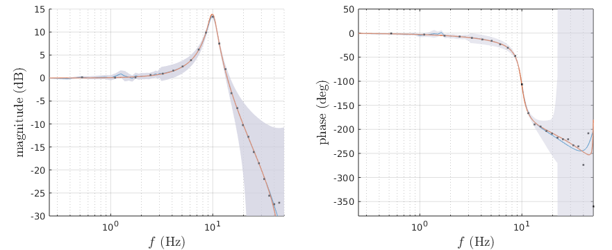
Figure 1: Bode plot of the second-order resonant system (orange), and its estimate (blue) using $H_{\infty}$ Gaussian process regression from an empirical transfer function estimate (black points) with $\eta=3$ confidence ellipsoid bounds (grey).

We now demonstrate the process by applying the strictly-linear $H_{\infty}$ Gaussian process regression method to the problem of identifying a second-order system that exhibits a resonance peak. The system is specified in continuous time, with canonical second-order transfer function

(11) $$g(s)=\frac{\omega_{0}^{2}}{s^{2}+2\xi\omega_{0}s+\omega_{0}^{2}},$$

where $\omega_{0}=20\pi$ rad/s, and $\xi=0.1$, and converted to the discrete-time transfer function $g(z)$ using a zero-order hold discretization with a sampling frequency of $f_{s}=100$ Hz. We suppose that we know a priori that there is a resonance peak, but not about its location or half-width, and we have no other strong information about the frequency response. For this prior belief, an appropriate prior model is a weighted mixture of a cozine process and a Hermitian stationary process. In particular, we use the family of $H_{\infty}$ processes with covariance functions

(12) $$k(z,w)=\sigma^{2}_{g}k_{g}(z,w)+\sigma^{2}_{c}k_{c}(z,w),\tilde{k}(z,w)=\sigma^{2}_{g}\tilde{k}_{g}(z,w)+\sigma^{2}_{c}\tilde{k}_{c}(z,w),$$

where $k_{g}$ is the covariance of the geometric $H_{\infty}$ process defined in Example 2.9, and $k_{c}$ is the covariance of the cozine process, and likewise for the complementary covariance. $\sigma^{2}_{g}$ and $\sigma^{2}_{c}$ are weights that determine the relative importance of the two parts of the model. This family of covariances has five hyperparameters: $\sigma_{g}\in[0,\infty)$, $\alpha\in(0,1)$, $\sigma_{c}\in[0,\infty)$, $\omega_{0}\in[0,\pi]$, and $a\in(0,1)$.

We suppose that an input trace $u(n)$ of Gaussian white noise with variance $\sigma^{2}_{u}=1/f_{s}$ is run through $H_{g}$ yielding an output trace $y(n)$; our observations comprise these two traces, corrupted by additive Gaussian white noise of variance $\sigma^{2}=10^{-4}/f_{s}$. To obtain an empirical transfer function estimate, we run both observation traces through a bank of 25 windowed 1000-tap DFT filters. The impulse responses of the filter bank are $h_{i}(n)=e^{j\omega_{i}n}w(n)$ for $i=1,\dotsc,25$, with Gaussian window $w(n)=\exp(-\tfrac{1}{2}(\sigma_{w}(n-500)/1000)^{2})$ for $n=0,\dotsc,999$, and $w(n)=0$ otherwise, with window half-width $\sigma_{w}=0.25$. Let $u_{i}$, $y_{i}$ denote the outputs of filter $h_{i}$ with inputs $u$, $y$ respectively: $y_{i}(n)/u_{i}(n)$ gives a running estimate of $g(e^{j\omega_{i}})$, whose value after 1000 time steps we take as our observation at $z_{i}=e^{j\omega_{i}}$. Figure 1 shows the regression from the strictly linear estimator (10) after tuning the covariance hyperparameters via maximum likelihood, along with predictive error bounds based on $\eta=3$ confidence ellipsoids.

4 Robustness Analysis with $H_{\infty}$ Gaussian Processes

Now that we have explored how to refine an $H_{\infty}$ GP model from online data, we move to a second and equally important problem: how to establish probabilistic robustness guarantees for $H_{\infty}$ processes. Our goal is to establish probabilistic guarantees of robustness; in other words, establishing that a given certificate of robustness is obtained with probability $\geq 1-\epsilon$ for a prescribed $\epsilon\in(0,1)$. For several classical robustness certificates, this reduces to the problem of bounding the gain excursion probability

$$P_{\gamma}(f)=\mathbb{P}\left(\sup_{\Omega\in[-\pi,\pi)}|f(e^{j\Omega})|>\gamma\right)$$

of a general $H_{\infty}$ GP $f$, which measures how likely the $L_{2}$ gain of $H_{f}$ is to exceed the level $\gamma$. A simple example of how excursion problems arise is the problem of extending small-gain arguments to the probabilistic case with an $H_{\infty}$ GP uncertainty. Consider a nominal plant $G$ in feedback with an uncertainty $\Delta$ modeled by an $H_{\infty}$ GP. Assume the plant satisfies $\lVert G\rVert_{\infty}<M$; then it follows from the small-gain condition [8, Theorem III.2.1] that the interconnection is stable if $\lVert\Delta\rVert_{\infty}\leq\frac{1}{M}\overset{\Delta}{=}\gamma$. Thus bounding $P_{\gamma}(\Delta)\leq\epsilon$ amounts to proving that the interconnection is stable for an ensemble of realizations with probability $\geq 1-\epsilon$.

A more general example is the problem of proving an probabilistic guarantee that an $H_{\infty}$ GP satisfies an integral quadratic constraint (IQC). In the discrete time SISO setting, an IQC with multiplier $\Pi$ is a behavioral constraint on signals $(v,w)\in H_{2}\times H_{2}$ of the form [12, 16, 26]

(13) $$\int_{-\pi}^{\pi}\begin{bmatrix}v(e^{j\Omega})\\ w(e^{j\Omega})\end{bmatrix}^{*}\Pi(e^{j\Omega})\begin{bmatrix}v(e^{j\Omega})\\ w(e^{j\Omega})\end{bmatrix}d\Omega\geq 0$$

where $\Pi:[-\pi,\pi)\to\mathbb{C}^{2\times 2}$. A conjugate-symmetric system $\Delta:H_{2}\to H_{2}$ is said to satisfy the IQC with a multiplier $\Pi$ if (13) is satisfied by pairs $(v,\Delta v)$ for all conjugate-symmetric $v\in H_{2}$. IQCs are able to express a wide range of behavioral properties, and knowing that an uncertainty satisfies a particular IQC is a powerful tool for constructing controllers that are robust against uncertainties satisfying that IQC.

If $\Delta$ is an LTI operator, then under fairly mild conditions, the IQC has a simple geometric interpretation. Specifically, the if $\Delta$ satisfies (13) then its frequency response $\Delta(e^{j\Omega})$ is constrained, pointwise in frequency, to lie: (a) within a circle if $\Pi_{22}(e^{j\Omega})<0$; (b) outside a circle if $\Pi_{22}(e^{j\Omega})>0$; or (c) on one side of a half space if $\Pi_{22}(e^{j\Omega})=0$. We shall state this result formally for case (a), but an analogous statement can be given for the other two cases. The result is provided under the assumption $\Pi_{22}(e^{j\Omega})=-1$. This normalization is without loss of generality because we can scale the multiplier $\Pi$ by a positive constant.

Lemma 4.1 (adapted from [17], Lemma 1 (i)).

Suppose that an LTI system with conjugate-symmetric transfer function $\Delta$ satisfies an IQC with continuous, conjugate-symmetric multiplier $\Pi$ normalized to $\Pi_{22}(e^{j\Omega})=-1$. Then for each $\Omega\in[-\pi,\pi)$, $\Delta(e^{j\Omega})$ lies in a circle in the Nyquist plane with center $\Pi_{21}(e^{j\Omega})$ and radius

$\sqrt{|\Pi_{11}(e^{j\Omega})|^{2}+|\Pi_{21}(e^{j\Omega})|^{2}}$.

This condition is evidently equivalent to the condition that

(14) $$\frac{|\Delta(e^{j\Omega})-\Pi_{21}(e^{j\Omega})|}{\sqrt{|\Pi_{11}(e^{j\Omega})|^{2}+|\Pi_{21}(e^{j\Omega})|^{2}}}\leq 1\ \forall\Omega\in[-\pi,\pi).$$

Thus the problem of establishing that an $H_{\infty}$ GP satisfies an IQC with probability $\geq 1-\epsilon$ reduces to a gain excursion probability problem, namely proving that

(15) $$\mathbb{P}\left(\sup_{\Omega\in[-\pi,\pi)}\left|\frac{\Delta(e^{j\Omega})-\Pi_{21}(e^{j\Omega})}{\sqrt{|\Pi_{11}(e^{j\Omega})|^{2}+|\Pi_{21}(e^{j\Omega})|^{2}}}\right|>1\right)\leq\epsilon,$$

or in other words that

(16) $$P_{1}\left(\frac{\Delta(e^{j\Omega})-\Pi_{21}(e^{j\Omega})}{\sqrt{\Pi_{11}(e^{j\Omega})+|\Pi_{21}(e^{j\Omega})|^{2}}}\right)\leq\epsilon.$$

4.1 Bounding the excursion probability

Having established how gain excursion probabilities arise in proving probabilistic safety guarantees for $H_{\infty}$ uncertainties, we turn to the problem of how to bound these probabilities. It is not generally possible to directly compute $P_{\gamma}(f)$; however, we can bound it from above using a related quantity, the expected number of gain upcrossings.

Associated to any $H_{\infty}$ Gaussian process is its gain process $|f(e^{j\Omega})|,\Omega\in[-\pi,\pi)$. Assuming that the gain process is differentiable with respect to $\Omega$, a gain upcrossing at level $\gamma$ is a value $\Omega_{c}$ such that $|f(e^{j{\Omega_{c}}})|=\gamma$ and $\tfrac{\partial}{\partial\Omega}|f(e^{j{\Omega_{c}}})|>0$. Under the assumptions given so far, there can be at most finitely many upcrossings, so the random variable $N_{\gamma}=\#\{\Omega\in[-\pi,\pi):|f(e^{j\Omega})|=\gamma\text{ and }\tfrac{\partial}{\partial\Omega}|f(e^{j\Omega})|>0\}$, where $\#S$ denotes the cardinality of a set $S$, is well-defined and its expectation $\mathbb{E}\left[N_{\gamma}\right]$ is almost surely finite. A simple application of Markov’s inequality yields the bound

(17) $$P_{\gamma}(f) =\mathbb{P}\left(|f(e^{j{0}})|>\gamma\right)+\mathbb{P}\left(|f(e^{j{0}})|\leq\gamma,N_{\gamma}\geq 1\right)$$

$$\leq\mathbb{P}\left(|f(e^{j{0}})|>\gamma\right)+\mathbb{E}\left[N_{\gamma}\right].$$

The reason that we consider a bound for $P_{\gamma}$ rather than a direct computation is that direct computation of $P_{\gamma}$ is only possible in the simplest cases. On the other hand, $\mathbb{E}\left[N_{\gamma}\right]$ can be computed with a closed-form (though sometimes complicated) expression as long as the process is differentiable.

The lack of Gaussian structure in $|f(e^{j\Omega})|$ would make it difficult to compute this formula directly from $f$ (e.g. by applying a Rice formula like [1, Theorem 3.4]). To overcome the difficulty, we reframe the problem as a vector crossing problem on the vector Gaussian process $g(\Omega)=(x(e^{j\Omega}),y(e^{j\Omega}))$ formed from the real and imaginary parts: the gain process $|f(e^{j\Omega})|$ crosses from $\leq\gamma$ to $>\gamma$ precisely when the vector process $g(\Omega)$ crosses from the interior of the circle $x^{2}+y^{2}=\gamma^{2}$ to the exterior. By taking this perspective, we relinquish the topological simplicity of the scalar crossing problem in order to retain the Gaussian structure of the stochastic process. While we cannot apply Rice formulas in the vector setting, there are analogous results for counting vector crossings. We use the following result due to Belyaev.

Theorem 4.2 (first-order Belyaev formula [3]).

Let $g:\Xi\times[0,T]\to\mathbb{R}^{n}$ be a vector-valued stochastic process and $\Phi:\mathbb{R}^{n}\to\mathbb{R}$ a boundary function satisfying the following conditions:

1. $g$ is continuously differentiable with probability one, and the random variables $g(t)$, $t\in T$ all possess densities $p_{g(t)}$;

2. The conditional densities $p(x|y)$ exist for $x=g(t)$, $y=g^{\prime}(t)$, and the densities depend continuously on $x$.

3. $\Phi$ is continuously differentiable, and to each $\epsilon$-neighborhood of the surface $S_{\Phi}=\{x\in\mathbb{R}^{n}:\Phi(x)=0\}$ we can associate coordinates $(\phi,\zeta_{1},\dotsc,\zeta_{n-1})$, where $\phi=\inf_{y\in S_{\Phi}}||x-y||_{2}$;

Let $N_{\Phi}$ denote the number of times a realization $g_{\xi}$ of $f$ exits the surface $S_{\Phi}$: then

(18) $$\mathbb{E}\left[N_{\Phi}\right]=\int_{0}^{T}\int_{S_{\phi}}\mathbb{E}\left[n{((x)}^{\top}g(t))_{+}|g^{\prime}(t)=x\right]p_{f(t)}(x)ds(x)dt,$$

where $(x)_{+}=\max(0,x)$, and $n(x)$ is the outward-facing unit normal vector of $S_{\Phi}$ at the point $x$.

Applying the first-order Belyaev formula to the real and imaginary parts of an $H_{\infty}$ GP and the surface $x^{2}+y^{2}=\gamma^{2}$ yields the following formula for the expected number of gain upcrossings, whose proof is deferred to Section 6.

Theorem 4.3.

Consider an $H_{\infty}$ Gaussian process $f$ with mean $m_{x}+jm_{y}$ and Hermitian and complementary covariances $k$, $\tilde{k}$. Let $N_{\gamma}$ denote the integer-valued random variable that counts the number of $\gamma$-level gain upcrossings of $f$. Suppose that $m_{x}(e^{j\Omega})$ and $m_{y}(e^{j\Omega})$ are differentiable with respect to $\Omega$ and that $k(e^{j{\Omega_{1}}},e^{j{\Omega_{2}}})$ and $\tilde{k}(e^{j{\Omega_{1}}},e^{j{\Omega_{2}}})$ are thrice differentiable with respect to $\Omega_{1}$ and $\Omega_{2}$. Then the expected number of gain upcrossings between frequencies $-\pi$ and $\pi$ is

(19) $$\mathbb{E}\left[N_{\gamma}\right] =\int_{-\pi}^{\pi}\int_{0}^{2\pi}\frac{\gamma}{2\pi}\Bigg{(}\frac{\sigma_{z(\theta)}(\Omega)}{\sqrt{2\pi}}e^{-\frac{1}{2}(\mu_{z(\theta)}(\Omega)/\sigma_{z(\theta)}(\Omega))^{2}}$$

$$\qquad\qquad\qquad+\frac{1}{2}\mu_{z(\theta)}(\Omega)\left(1+\operatorname{erf}\left(\frac{\mu_{z(\theta)}(\Omega)}{\sqrt{2}\sigma_{z(\theta)}(\Omega)}\right)\right)\Bigg{)}$$

$$\times\det\Sigma(\Omega,\Omega)^{-1/2}e^{-\frac{1}{2}(z(\theta)-m(\Omega))^{\top}\Sigma(\Omega,\Omega)^{-1}(z(\theta)-m(\Omega)}d\theta d\Omega,$$

where

(20) $$z(\Omega) =[\gamma\cos(\Omega);\gamma\sin(\Omega)]$$

(21) $$\mu_{z}(\Omega) =\gamma^{-1}z^{\top}m(\Omega)^{\prime}+\gamma^{-1}z^{\top}C(\Omega,\Omega)\Sigma(\Omega,\Omega)^{-1}(z-m(\Omega))$$

(22) $$\sigma_{z}(\Omega) =\gamma^{-2}z^{\top}(\Sigma^{\prime}(\Omega,\Omega)-C(\Omega,\Omega)(\Sigma(\Omega,\Omega)^{-1}C(\Omega,\Omega)^{\top})z$$

(23) $$\Sigma(\Omega,\Omega) =\begin{bmatrix}k_{x}(\Omega,\Omega)&k_{c}(\Omega,\Omega)\\ k_{c}(\Omega,\Omega)&k_{y}(\Omega,\Omega)\end{bmatrix},\Sigma^{\prime}(\Omega,\Omega)=\begin{bmatrix}k_{x}^{12}(\Omega,\Omega)&k_{c}^{12}(\Omega,\Omega)\\ k_{c}^{12}(\Omega,\Omega)&k_{y}^{12}(\Omega,\Omega)\end{bmatrix},$$

(24) $$C(\Omega,\Omega) =\begin{bmatrix}k_{x}^{1}(\Omega,\Omega)&k_{c}^{1}(\Omega,\Omega)\\ k_{c}^{2}(\Omega,\Omega)&k_{y}^{1}(\Omega,\Omega)\end{bmatrix},m(\Omega)=\begin{bmatrix}m_{x}(e^{j\Omega})\\ m_{y}(e^{j\Omega})\end{bmatrix},$$

(25) $$k_{x}(\Omega_{1},\Omega_{2}) =\tfrac{1}{2}\operatorname{Re}\left[k(e^{j{\Omega_{1}}},e^{j{\Omega_{2}}})+\tilde{k}(e^{j{\Omega_{1}}},e^{j{\Omega_{2}}})\right]$$

(26) $$k_{y}(\Omega_{1},\Omega_{2}) =\tfrac{1}{2}\operatorname{Re}\left[k(e^{j{\Omega_{1}}},e^{j{\Omega_{2}}})-\tilde{k}(e^{j{\Omega_{1}}},e^{j{\Omega_{2}}})\right]$$

(27) $$k_{c}(\Omega_{1},\Omega_{2}) =\tfrac{1}{2}\operatorname{Im}\left[\tilde{k}(e^{j{\Omega_{1}}},e^{j{\Omega_{2}}})-k(e^{j{\Omega_{1}}},e^{j{\Omega_{2}}})\right]$$

and where the superscripts denote derivatives, e.g. $k_{x}^{12}=\partial^{2}k_{x}/\partial\Omega_{1}\Omega_{2}.$

Remark 4.4.

If $f$ is conjugate-symmetric, then $|f|$ is an even function of $\Omega$, meaning that the probability of a gain bound violation over $\Omega\in[-\pi,\pi)$ is equal to the violation probability over the reduced range $\Omega\in[0,\pi]$. In this case, we need only compute the expected number of gain upcrossings between $0$ and $\pi$, and the lower limit of the outer integral in (19) can be changed from $-\pi$ to zero.

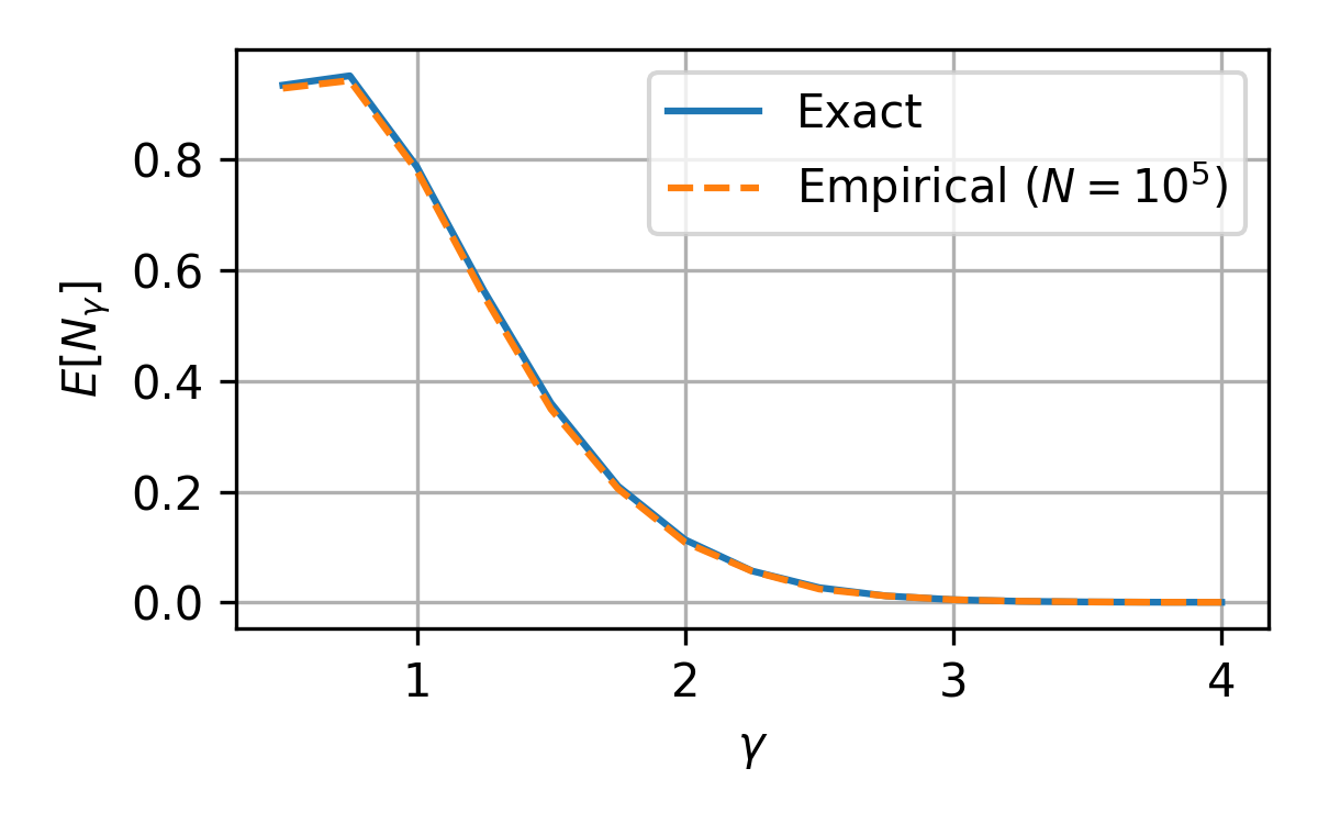
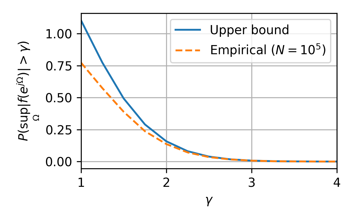
Figure 2: Evaluating the Belyaev formula and the excursion gain bound on a geometric $H_{\infty}$ process with $\alpha=0.5$. Left: Numerical comparison of (18) with an empirical estimate ($N=100,000$) of $\mathbb{E}\left[N_{\gamma}\right]$. Right: Numerical comparison of (17) with an empirical estimate ($N=100,000$) of $P_{\gamma}(f)$.

We next use a simple example to numerically demonstrate the validity of the gain upcrossing formula (19) and to test the tightness of the bound (17). Our example uses a geometric $H_{\infty}$ GP $f$ with $\alpha=0.5$ (Example 2.9) and a range of threshold values $\gamma\in[1,4]$. The expected $H_{2}$ norm of a geometric $H_{\infty}$ process is $1$, so it’s reasonable to expect $\mathbb{E}\left[N_{\gamma}\right]$ and $P_{\gamma}(f)$ to be relatively high near $\gamma=1$, and to taper off relatively quickly. Figure 2 shows the results of the numerical evaluation of Equations (19), (17) and compares the results to empirical approximations of $\mathbb{E}\left[N_{\gamma}\right]$ and $P_{\gamma}(f)$ made using $N=100,000$ process realizations. We can conclude from the figure that (18) accurately computes $\mathbb{E}\left[N_{\gamma}\right]$ as expected. Furthermore, we see that (17) indeed upper bounds $P_{\gamma}\gamma(f)$; while the bound is conservative in regions where $P_{\gamma}(f)$ is high, it quickly becomes tighter where $P_{\gamma}(f)$ is small, levelling off to overestimate $P_{\gamma}(f)$ by $\sim 10\%$ for $\gamma>2.5$. Since we will generally engineer $P_{\gamma}(f)$ to be small in applications, the experiment shows that (17) is not a conservative bound in regions of practical interest.

5 Conclusion

This paper has three principal contributions: how to construct $H_{\infty}$ GPs, how to refine an $H_{\infty}$ GP model with data, and how to prove robustness guarantees for systems with probabilistic $H_{\infty}$ feedback uncertainties. The fact that $H_{\infty}$ GPs are amenable both to regression and rigorous robustness analysis is a critical advantage in applications calling for robustly safe learning of uncertainties of a priori unknown order; such uncertainties frequently arise when flexible mechanics (e.g. flexible modes, aeroelastic coupling, soft robotic parts) are neglected in the nominal plant.

The regression-based refinement method described in Section 3 depends strongly on the method used to convert time-domain data to frequency-domain, many of which (such as filter banks and ETFEs) are sensitive to measurement noise. A more direct application of time-domain data to the frequency-domain model, perhaps effected by a projected-process regression [21, §8.3.4]. Even within the regime of refinement via frequency-domain data, there remains some mystery around the performance gap between strictly linear and widely linear estimators. We conjecture that the similarity in performance is due to the perfect correlation between real and imaginary parts of the transfer function induced by via the discrete Hilbert transform (see [20], §2.26) induced by the symmetry condition required for the process to give real outputs to real inputs. In the large-sample limit, this condition causes the prior regression covariance to become maximally improper, a special case in which the strictly linear estimator is indeed optimal.

A key direction for future work is to extend $H_{\infty}$ GP regression and Belyaev-based bounds on excursion probabilities to the MIMO case. MIMO regression should pose little difficulty; a simple tactic, if no better can be found, is to perform regression independently on each element of a transfer function matrix. For MIMO excursion bounds, such an independent approach would likely not be as effective; instead we would need to directly examine MIMO gains (e.g. by a probabilistic extension of sigma plots) or direct examination of probabilistic IQCs. In either case, the near-Gaussian structure enjoyed in the SISO case will likely not hold, so a more general theory of excursion probabilities will be necessary.

6 Proofs of Main Results

Proof 6.1 (Proof of Lemma 2.1).

We begin by constructing a proper z-domain process $f$ with covariance $k$ from an orthonormal basis for the reproducing kernel Hilbert space $\mathcal{H}\!\left(k\right)$. Then, we establish that $f$ has a mean-square derivative $f_{1}$ that has a continuous version. Finally, we use $f_{1}$ and a point evaluation $f(z_{0})$ to construct a process $g$ that has complex differentiable (i.e. holomorphic and therefore analytic) sample paths, which we then show is pointwise identical to $f$.

Since $k$ is a forteriori continuous, $\mathcal{H}\!\left(k\right)$ is separable and admits a countable orthonormal basis $\{\phi_{n}\}_{n=0}^{\infty}$, and we can express $k$ as the pointwise and uniformly converging sum $k(z,w)=\sum_{n=0}^{\infty}\phi_{n}(z)\phi^{*}_{n}(w).$ Let $\{a_{n}\}_{n=0}^{\infty}$, $\{b_{n}\}_{n=0}^{\infty}$ denote two sequences of independent standard normals, that is $a_{1},b_{1},a_{2},b_{2},\dotsc\overset{\textrm{i.i.d.}}{\sim}\mathcal{N}\left(0,1\right)$. Then the random function $f(z)=\sum_{n=0}^{\infty}\frac{1}{\sqrt{2}}(a_{n}+jb_{n})\phi_{n}(z)$ is a z-domain Gaussian process on the set of $z$ where the sum converges. From the summation form of $f$ we can verify $\mathbb{E}\left[f(z)f(w)^{*}\right]=k(z,w),$ $\mathbb{E}\left[f(z)f(w)\right]=0,$ making $f$ a proper z-domain process where it exists; and since $k(z,z)$ is finite for all $z\in D$, it follows that the pointwise sums $f(z)$ converge for all $z\in D$.

We now prove that $f$ admits a version $g$ whose realizations are analytic. To do so, we demonstrate that $f$ admits a mean-square derivative $f_{1}$ which admits a continuous version, which we then use to construct a version of $f$ that is holomorphic and therefore analytic.

For the real-domain case, it is well known that a stochastic process possesses a mean-square derivative if its covariance function is twice differentiable, and that the covariance of the mean-square derivative is the first derivative of the covariance with respect to both arguments [15, §34]. The complex-domain case is nearly the same, except that the derivative with respect to the second argument must be a conjugate derivative. Specifically, suppose that the limit

(28) $$\lim_{z\to z_{0},w\to w_{0}}\mathbb{E}\left[\left(\frac{f(z)-f(z_{0})}{z-z_{0}}\right)\left(\frac{f(w)-f(w_{0})}{w-w_{0}}\right)^{*}\right]$$

$$=\lim_{z\to z_{0},w\to w_{0}}\frac{k(z,w)-k(z,w_{0})-k(z_{0},w)+k(z_{0},w_{0})}{(z-z_{0})(w-w_{0})^{*}}=\frac{\partial^{2}}{\partial z\partial w^{*}}k$$

exists for all $z_{0},w_{0}\in D$: then any proper z-domain process $f_{1}$ with Hermitian covariance $\frac{\partial^{2}}{\partial z\partial w^{*}}k$ is a mean-square derivative of $f$, since it satisfies the mean-square differentiability criterion $\lim_{z\to z_{0}}\mathbb{E}\left[\left|\frac{f(z)-f(z_{0})}{z-z_{0}}\right|-f_{1}(z_{0})\right]=0$. By our assumption that $k$ is holomorphic in the first argument and antiholomorphic in the second argument, it follows that $k$ possesses derivatives in the first argument, and conjugate derivatives in the second argument, of all orders; let $k_{nm}$ denote the derivative of $k$ taken $n$ times in the first argument and the conjugate derivative $m$ times in the second argument. In particular, the existence of $k_{11}$ means that $f$ indeed possesses a mean square derivative $f_{1}$ as described above.

Since $f_{1}$ is mean zero and proper, it follows that its real and imaginary parts ($x_{1}$ and $y_{1}$ respectively) are independent and identical real Gaussian processes with mean zero, and calculation from the relation $x_{1}=\frac{1}{2}(f_{1}+f_{1}^{*})$ yields the covariance

$$\mathbb{E}\left[x_{1}(z)x_{1}(w)\right]=\operatorname{Re}\left[k_{11}(z,w)\right].$$

From this it follows that $x_{1}$ has the canonical metric

$$d^{2}_{x_{1}}(z,w)=\mathbb{E}\left[(x_{1}(z)-x_{1}(w))^{2}\right]=k_{11}(z,z)+k_{11}(w,w)-2k_{11}(z,w).$$

By assumption we then have $d^{2}_{x_{1}}(z,w)\leq|z-w|^{2+\alpha},$ and from [1, prop. 1.16] it follows that $x_{1}$ admits a version with continuous sample paths. Evidently the same is true for $y_{1}$, being identically distributed to $x_{1}$, which means that $f_{1}$ admits a continuous version. Define $g$ as the z-domain process whose realizations are formed as $g_{\xi}(z)=f(z_{0})+\int_{\gamma}f_{1,\xi}(\zeta)d\zeta,$ where $f_{1,\xi}$ is a realization of the continuous version of $f_{1}$, $z_{0}\in D$ and $\gamma$ is a continuous path starting at $z_{0}$ and ending at $z$. The realizations $g_{\xi}$ evidently possess derivatives; by the fundamental theorem of calculus we have $\frac{d}{dz}g_{\xi}=f_{1,\xi}$, which is continuous and therefore bounded on the compact domain $D$. We now show that $g$ is in fact a version of $f$ by showing that

$$\mathbb{E}\left[|f(z)-g(z)|^{2}\right] =\mathbb{E}\left[f(z)f(z)^{*}-f(z)g(z)^{*}-g(z)f(z)^{*}+g(z)g(z)^{*}\right]$$

$$=k(z,z)-\mathbb{E}\left[f(z)g(z)^{*}\right]-\mathbb{E}\left[g(z)f(z)^{*}\right]+\mathbb{E}\left[g(z)g(z)^{*}\right]=0.$$

For the second term we have

$$\mathbb{E}\left[f(z)g(z)^{*}\right] =\mathbb{E}\left[f(z)f(z_{0})^{*}+f(z)\int_{\gamma}f_{1}(\zeta)^{*}d\zeta^{*}\right]$$

$$=\mathbb{E}\left[f(z)f(z_{0})^{*}\right]+\int_{\gamma}\mathbb{E}\left[f(z)f_{1}(\zeta)\right]d\zeta^{*}=k(z,z_{0})+\int_{\gamma}k_{01}(z,\zeta)d\zeta^{*}$$

$$=k(z,z),$$

where the last line follows from the fact that $k$ is a complex antiderivative for $k_{01}$. The third term immediately follows since

$$\mathbb{E}\left[g(z)f(z)^{*}\right]=\mathbb{E}\left[f(z)g(z)^{*}\right]^{*}=k(z,z)^{*}=k(z,z).$$

For the final term we have

$$\mathbb{E}\left[g(z)g(z)^{*}\right] =\mathbb{E}\left[f(z_{0})f(z_{0})^{*}+f(z_{0})\int_{\gamma}f_{1}(\zeta)^{*}d\zeta^{*}\right]$$

$$\quad+\mathbb{E}\left[f(z_{0})^{*}\int_{\gamma}f_{1}(\zeta)d\zeta+\left(\int_{\gamma}f_{1}(\zeta)d\zeta\right)\left(\int_{\gamma}f_{1}(\zeta)^{*}d\zeta^{*}\right)\right]$$

$$=\mathbb{E}\left[f(z_{0})f(z_{0})^{*}\right]+\int_{\gamma}\mathbb{E}\left[f(z_{0})f_{1}(\zeta)^{*}\right]d\zeta^{*}+\int_{\gamma}\mathbb{E}\left[f(z_{0})^{*}f_{1}(\zeta)\right]d\zeta$$

$$\quad+\int_{\gamma}\int_{\gamma}\mathbb{E}\left[f(\zeta_{1})f(\zeta_{2})^{*}\right]d\zeta_{1}d\zeta_{2}^{*}$$

$$=k(z_{0},z_{0})+\int_{\gamma}k_{01}(z_{0},\zeta)d\zeta+\int_{\gamma}k_{01}(z_{0},\zeta)^{*}d\zeta+\int_{\gamma}\int_{\gamma}k_{11}(\zeta_{1},\zeta_{2})d\zeta_{1}d\zeta_{2}$$

$$=k(z_{0},z_{0})+(k(z_{0},z)-k(z_{0},z_{0}))+(k(z_{0},z)^{*}-k(z_{0},z_{0})^{*})$$

$$+(k(z,z)-k(z,z_{0})-k(z_{0},z)+k(z_{0},z_{0}))=k(z,z).$$

Note that the exchange of the double integral is permitted by Fubini’s theorem since realizations of $f_{1}$ are bounded. We have also used the Hermitian covariance properties $k(z,w)=k(w,z)^{*}$, $k(z,z)=k(z,z)^{*}$. Putting the terms together, we arrive at

$$\mathbb{E}\left[|f(z)-g(z)|^{2}\right] =k(z,z)-k(z,z)-k(z,z)+k(z,z)=0,$$

proving that $g$ is a version of $f$.

Proof 6.2 (Proof of Theorem 2.8).

First, we show that $f$ having the form (6) with positive $\{a_{n}\}_{n=0}^{\infty}\in\ell^{1}$ implies that $f$ is a conjugate-symmetric and Hermitian stationary $H_{\infty}$ process with the given covariances. Suppose that $f(z)=\sum_{n=0}^{\infty}a_{n}w_{n}z^{-n}$. We can readily see that

(29) $$k(z,w) =\mathbb{E}\left[f(z)f(w)^{*}\right]=\mathbb{E}\left[\left(\sum_{n=0}^{\infty}a_{n}w_{n}z^{-n}\right)\left(\sum_{m=0}^{\infty}a_{m}w_{m}(w)^{-m}\right)^{*}\right]$$

$$=\mathbb{E}\left[\sum_{n=0,m=0}^{\infty}a_{n}a_{m}w_{n}w_{m}z^{-n}(w^{*})^{-n}\right]=\sum_{n=0}^{\infty}a_{n}^{2}(zw^{*})^{-n},$$

where the cross terms vanish by the independence of the $w_{n}$. Conjugate symmetry follows from the direct calculation $f(z)^{*}=(\sum_{n=0}^{\infty}a_{n}w_{n}z^{-n})^{*}=\sum_{n=0}^{\infty}a_{n}w_{n}(z^{*})^{-n}=f(z^{*})$. Since $f$ is conjugate symmetric, its realizations represent systems with a real-valued impulse response when interpreted as transfer functions. Recall that a SISO LTI system is BIBO stable if and only if its impulse response is absolutely summable. To that end, consider the sequence $M_{T}=\sum_{n=0}^{T}|h_{f}(n)|=\sum_{n=0}^{T}a_{n}|w_{n}|$ of partial sums: if $\lim_{T\to\infty}M_{T}$ converges to a random variable that is finite with probability one, then the impulse response is absolutely summable with probability one. Since the $w_{n}$ are independent and $0<a_{n}|w_{n}|<\infty$ for all $n$, it follows that $M_{T}$ is a submartingale and that $\mathbb{E}\left[M_{T}\right]$ increases monotonically. Using the summability condition on the $a_{n}$ and the fact that $\mathbb{E}\left[|w_{n}|\right]=\sqrt{2/\pi}$ (as $|w_{n}|$ follows a half-normal distribution), we have

(30) $$\mathbb{E}\left[\sum_{n=0}^{\infty}|h_{f}(n)|\right]=\sum_{n=0}^{\infty}a_{n}|w_{n}|=\sqrt{\frac{2}{\pi}}\sum_{n=0}^{\infty}a_{n}<\infty,$$

which means $\sup_{T}\mathbb{E}\left[M_{T}\right]<\infty$ by monotonicity. Since $M_{T}$ is a submartingale and $\sup_{T}\mathbb{E}\left[M_{T}\right]$ is finite, it follows by the Martingale convergence theorem [10, Theorem 4.2.11] that the limit of $M_{T}$ converges to a random variable that is finite with probability one. This shows that $h_{f}$ is absolutely summable with probability one, implying BIBO stability and that $f\in H_{\infty}$ with probability one.

Next, we show that a Hermitian stationary, conjugate-symmetric $H_{\infty}$ Gaussian process $f$ must have Hermitian and complementary covariances of the form (5), and that this in turn implies that $f$ has the form (6). Since $f\in H_{\infty}$, we can use the fact that $z^{-n},n\geq 0$ is a basis for $H_{\infty}$ to expand $f$ as $f(z)=\sum_{n=0}^{\infty}h_{n}z^{-n},$ where the coefficients $h_{n}=\langle f,z^{-n}\rangle_{2}$ are an infinite sequence of random variables. Since $f$ is Gaussian and conjugate symmetric, the $h_{n}$ are real Gaussian random variables that may be correlated. From this form, we can express the Hermitian and complementary covariance as

(31) $$k(z,w)=\sum_{n=0}^{\infty}\sum_{m=0}^{\infty}\mathbb{E}\left[h_{n}h_{m}\right]z^{-n}(w^{*})^{-m},$$

(32) $$\tilde{k}(z,w)=\sum_{n=0}^{\infty}\sum_{m=0}^{\infty}\mathbb{E}\left[h_{n}h_{m}\right]z^{-n}(w)^{-m},$$

which shows that $\tilde{k}(z,w)=k(z,w^{*})$ for $z,w\in E^{2}$. Restricting the covariance functions to the unit circle, we have

(33) $$k(e^{j\theta},e^{j\phi}) =\sum_{n=0}^{\infty}\sum_{m=0}^{\infty}\mathbb{E}\left[h_{n}h_{m}\right]e^{-j(n\theta-m\phi)}$$

$$\tilde{k}(e^{j\theta},e^{j\phi}) =\sum_{n=0}^{\infty}\sum_{m=0}^{\infty}\mathbb{E}\left[h_{n}h_{m}\right]e^{-j(n\theta+m\phi)}.$$

By the assumption of Hermitian stationarity, we know that $k(e^{j(\theta-\phi)},1)$ is a positive definite function whose domain is the unit circle. We can therefore apply Bochner’s theorem [22, section 1.4.3] to obtain a second expansion

(34) $$k(e^{j(\theta-\phi)},1)=k(e^{j\theta},e^{j\phi})=\sum_{n\in\mathbb{Z}}a_{n}^{2}e^{-jn(\theta-\phi)},$$

where $a_{n}$ are real and nonnegative. In order for the expansion of $k$ in (33) and the expansion in (34) to be equal, the positive-power terms in (34) must vanish, and the cross-terms in (33) must vanish.

This means that $\mathbb{E}\left[h_{n}h_{m}\right]=0$ for $m\neq n$, from which it follows that the covariances have the form

(35) $$k(z,w) =\sum_{n=0}^{\infty}\mathbb{E}\left[h_{n}^{2}\right](zw^{*})^{-n}=\sum_{n=0}^{\infty}a_{n}^{2}(zw^{*})^{-n}$$

$$\tilde{k}(z,w) =\sum_{n=0}^{\infty}\mathbb{E}\left[h_{n}^{2}\right](zw)^{-n}=\sum_{n=0}^{\infty}a_{n}^{2}(zw)^{-n}$$

where we identify $a_{n}^{2}=\mathbb{E}\left[h_{n}^{2}\right]$, and that the $h_{n}$ are independent. Returning to the expanded form of the process and expressing $\mathbb{E}\left[h_{n}^{2}\right]=a_{n}^{2}$, we have $f(z)=\sum_{n=0}^{\infty}w_{n}a_{n}z^{-n}$ where $w_{n}\overset{\textrm{i.i.d.}}{\sim}\mathcal{N}\left(0,1\right)$.

Evidently, the impulse response $h_{f}$ has the same form as before, so the expected absolute sum of the impulse response is $\mathbb{E}\left[\sum_{n=0}^{\infty}|h_{f}(n)|\right]=\sqrt{\frac{2}{\pi}}\sum_{n=0}^{\infty}a_{n}$. Since $f\in H_{\infty}$ by assumption, it follows that $\sum_{n=0}^{\infty}|h_{f}(n)|$ almost surely converges, and therefore that $\mathbb{E}\left[\sum_{n=0}^{\infty}|h_{f}(n)|\right]<\infty$ by the Kolmogorov three-series theorem ([10, Theorem 2.5.8], condition (ii)), showing that $\{a_{n}\}_{n=0}^{\infty}\in\ell^{1}$.

Proof 6.3 (Proof (of Theorem 4.3)).

To apply Belyaev’s formula, we must first establish that the conditions of Theorem 4.2 are satisfied by the vector GP $g$ composed of the real and imaginary parts of $f$. That $g(e^{j\Omega})$ and $g^{\prime}(e^{j\Omega})|g(e^{j\Omega})$ have distributions is given by the fact that $g$ is a Gaussian process: $g(e^{j\Omega})$ is Gaussian-distributed by definition; the derivative of a Gaussian process is itself a Gaussian process; and a Gaussian random variable conditioned on another Gaussian random variable is itself Gaussian. The given conditions on differentiability ensure that $g$ is differentiable: a mean-zero process with thrice-differentiable covariances is at least once-differentiable, and adding a differentiable mean to the process preserves this property. Finally, the surface $x^{2}+y^{2}-\gamma^{2}=0$ satisfies the third condition, as an $\epsilon$-neighborhood of $S_{\phi}$ is simply an annulus in the plane with inner radius $\gamma-\epsilon$ and outer radius $\gamma+\epsilon$, which can be parameterized using polar coordinates.

With these conditions established, we know that the expected number of $\gamma$-level gain upcrossings of $f$ is given by (18) with $g=(x,y)$ and $\Phi(x,y)=x^{2}+y^{2}-\gamma^{2}$; all that remains is to show how to express (18) in terms computable from $k$, $\tilde{k}$, and $m$, that is to derive (19). First, there is the matter of integration over $S_{\Phi}$: this can be handled by integrating over its circular parameterization $S_{\Phi}=\{(\gamma\cos\theta,\gamma\sin\theta),\theta\in[-\pi,\pi)\}$ in which case $z=z(\theta)=(\gamma\sin\theta,\gamma\cos\theta),\quad ds(z)=\gamma d\theta.$ To obtain the distribution $p_{g(\Omega)}$, we require the first- and second-order statistics of $g$. Since the real and imaginary parts of $f$ are Gaussian, it follows that $g$ is a vector Gaussian process. Its mean and variance are

(36) $$\mathbb{E}\left[g(e^{j\Omega})\right]=\begin{bmatrix}\mathbb{E}\left[x(e^{j\Omega})\right]\\ \mathbb{E}\left[y(e^{j\Omega})\right]\end{bmatrix}=m(\Omega),\quad\Sigma(\Omega_{1},\Omega_{2})=\begin{bmatrix}k_{x}(\Omega_{1},\Omega_{2})&k_{c}(\Omega_{1},\Omega_{2})\\ k_{c}(\Omega_{1},\Omega_{2})&k_{y}(\Omega_{1},\Omega_{2})\\ \end{bmatrix},$$

which can be verified by substituting $x(e^{j\Omega})=\frac{1}{2}(f(e^{j\Omega})+f(e^{j\Omega})^{*}),$ $y(e^{j\Omega})=\frac{1}{2j}(f(e^{j\Omega})-f(e^{j\Omega})^{*}),$ and working out the expectations. From this, it follows that

(37) $$p_{f(\Omega)}(z)=(2\pi)^{-1}\Sigma(\Omega,\Omega)e^{-\tfrac{1}{2}(z-m(\Omega))^{\top}\Sigma(\Omega,\Omega)(z-m(\Omega))}.$$

To compute the conditional expectation, we also require the joint distribution of $g(\Omega)$ and its derivative $g^{\prime}(\Omega)$: this is another multivariate normal; this is

(38) $$\begin{bmatrix}g^{\prime}(\Omega)\\ g(\Omega)\end{bmatrix}\sim\mathcal{N}\left(\begin{bmatrix}m_{x}^{\prime}(\Omega)\\ m_{y}^{\prime}(\Omega)\\ m_{x}(\Omega)\\ m_{y}(\Omega)\end{bmatrix},\begin{bmatrix}\Sigma^{\prime}(\Omega,\Omega)&C(\Omega,\Omega)\\ C^{\top}(\Omega,\Omega)&\Sigma(\Omega,\Omega)\end{bmatrix}\right).$$

We next compute the conditional distribution of $g$ given $g^{\prime}=z$; this is again a multivariate normal: dropping $\Omega$ from the submatrices for brevity, we have

(39) $$g(\Omega)|g^{\prime}(\Omega)=z\sim\mathcal{N}\left(m^{\prime}+C\Sigma^{-1}(z-m),\Sigma^{\prime}-C\Sigma^{-1}C^{\top}\right).$$

The normal vector $n_{\Phi}(z)$ for $\Phi$—a circle with center zero and radius $\gamma$—is simply $\gamma^{-1}z$. Thus the linear mapping $(g(\Omega)|g^{\prime}(\Omega)=z)\mapsto n_{\Phi}(z)^{\top}(g(\Omega)|g^{\prime}(\Omega)=z)$ gives us the distribution

(40) $$n_{\Phi}(z)^{\top}(g(\Omega)|g^{\prime}(\Omega)=z)$$

$$\quad\sim\mathcal{N}\left(\gamma^{-1}z^{\top}m^{\prime}+\gamma^{-1}z^{\top}C\Sigma^{-1}(z-m),\gamma^{-2}z^{\top}(\Sigma^{\prime}-C(\Sigma^{-1}C^{\top})z\right)$$

$$\quad\overset{\Delta}{=}\mathcal{N}\left(\mu_{z}(\Omega),\sigma^{2}_{z}(\Omega)\right).$$

The remaining step is to compute the expectation of the positive part. Since $n_{\Phi}(z)^{\top}(g(\Omega)|g^{\prime}(\Omega)=z)$ is a Gaussian scalar, the positive part is a rectified Gaussian, whose mean is

(41) $$\mathbb{E}\left[(n_{\Phi}(z)^{\top}(g(\Omega))_{+}|g^{\prime}(\Omega)=z)\right] =\frac{\sigma_{z}(\Omega)}{\sqrt{2\pi}}e^{-\frac{1}{2}(\mu_{z}(\Omega)/\sigma_{z}(\Omega))^{2}}$$

$$+\frac{1}{2}\mu_{z}(\Omega)\left(1+\operatorname{erf}\left(\frac{\mu_{z}(\Omega)}{\sqrt{2}\sigma_{z}(\Omega)}\right)\right).$$

Finally, applying (37) and (41) to the Belyaev formula (18) yields the expression (19).

References

- [1] J.-M. Azaïs and M. Wschebor, Level sets and extrema of random processes and fields, John Wiley & Sons, 2009.
- [2] G. Balas, P. Seiler, and A. Packard, Analysis of an UAV flight control system using probabilistic , in AIAA Guidance, Navigation, and Control Conference, 2012, p. 4989.
- [3] Y. K. Belyaev, On the number of exits across the boundary of a region by a vector stochastic process, Theory of Probability & Its Applications, 13 (1968), pp. 320–324.
- [4] J.-M. Biannic, C. Roos, S. Bennani, F. Boquet, V. Preda, and B. Girouart, Advanced probabilistic -analysis techniques for AOCS validation, European Journal of Control, 62 (2021), pp. 120–129.
- [5] G. C. Calafiore and M. C. Campi, The scenario approach to robust control design, IEEE Transactions on automatic control, 51 (2006), pp. 742–753.
- [6] G. C. Calafiore and F. Dabbene, Probabilistic robust control, in 2007 American Control Conference, IEEE, 2007, pp. 147–158.
- [7] T. Chen, H. Ohlsson, and L. Ljung, On the estimation of transfer functions, regularizations and Gaussian processes—revisited, Automatica, 48 (2012), pp. 1525–1535.
- [8] C. A. Desoer and M. Vidyasagar, Feedback systems: input-output properties, SIAM, 2009.
- [9] A. Devonport, P. Seiler, and M. Arcak, Frequency domain Gaussian process models for H∞ uncertainties, in Learning for Dynamics and Control Conference, PMLR, 2023, pp. 1046–1057.
- [10] R. Durrett, Probability: theory and examples, vol. 49, Cambridge University Press, 2019.
- [11] M. H. Hayes, Statistical digital signal processing and modeling, John Wiley & Sons, 1996.
- [12] B. Hu, M. J. Lacerda, and P. Seiler, Robustness analysis of uncertain discrete-time systems with dissipation inequalities and integral quadratic constraints, International Journal of Robust and Nonlinear Control, 27 (2017), pp. 1940–1962.
- [13] S. Khatri and P. A. Parrilo, Guaranteed bounds for probabilistic , in Proceedings of the 37th IEEE Conference on Decision and Control (Cat. No. 98CH36171), vol. 3, IEEE, 1998, pp. 3349–3354.
- [14] J. Lataire and T. Chen, Transfer function and transient estimation by Gaussian process regression in the frequency domain, Automatica, 72 (2016), pp. 217–229.
- [15] M. Loève, Probability Theory, Dover, 2017.
- [16] A. Megretski and A. Rantzer, System analysis via integral quadratic constraints, IEEE transactions on automatic control, 42 (1997), pp. 819–830.
- [17] H. Pfifer and P. Seiler, Integral quadratic constraints for delayed nonlinear and parameter-varying systems, Automatica, 56 (2015), pp. 36–43.
- [18] G. Pillonetto, T. Chen, A. Chiuso, G. De Nicolao, and L. Ljung, Regularized system identification: Learning dynamic models from data, Springer Nature, 2022.
- [19] G. Pillonetto and G. De Nicolao, A new kernel-based approach for linear system identification, Automatica, 46 (2010), pp. 81–93.
- [20] L. R. Rabiner and B. Gold, Theory and application of digital signal processing, Englewood Cliffs: Prentice-Hall, (1975).
- [21] C. E. Rasmussen and C. K. Williams, Gaussian Processes for Machine Learning, MIT Press, 2006.
- [22] W. Rudin, Fourier analysis on groups, Interscience, 1962.
- [23] P. J. Schreier and L. L. Scharf, Statistical signal processing of complex-valued data: the theory of improper and noncircular signals, Cambridge University Press, 2010.
- [24] F. Somers, S. Thai, C. Roos, J.-M. Biannic, S. Bennani, V. Preda, and F. Sanfedino, Probabilistic gain, phase and disk margins with application to AOCS validation, IFAC-PapersOnLine, 55 (2022), pp. 1–6.
- [25] J. G. Stoddard, G. Birpoutsoukis, J. Schoukens, and J. S. Welsh, Gaussian process regression for the estimation of generalized frequency response functions, Automatica, 106 (2019), pp. 161–167.
- [26] J. Veenman, C. W. Scherer, and H. Köroğlu, Robust stability and performance analysis based on integral quadratic constraints, European Journal of Control, 31 (2016), pp. 1–32.