Matroid Stratification of
ML Degrees of Independence Models

Abstract

We study the maximum likelihood (ML) degree of discrete exponential independence models and models defined by the second hypersimplex. For models with two independent variables, we show that the ML degree is an invariant of a matroid associated to the model. We use this description to explore ML degrees via hyperplane arrangements. For independence models with more variables, we investigate the connection between the vanishing of factors of its principal $A$-determinant and its ML degree. Similarly, for models defined by the second hypersimplex, we determine its principal $A$-determinant and give computational evidence towards a conjectured lower bound of its ML degree.

1 Introduction

In this paper we study the maximum likelihood (ML) degree [CHKS06] of discrete exponential models in two instances: independence models and models defined by the second hypersimplex. Discrete exponential models are closely related to toric varieties [Sul18, Section 6.2]. Let

$$A=\begin{pmatrix}a_{1}&a_{2}&\cdots&a_{n}\end{pmatrix},$$

where $a_{i}\in\mathbb{Z}^{d}$, be a $d\times n$ integer matrix whose row-span contains the all-ones vector. For $w\in(\mathbb{C}^{*})^{n}$, the scaled toric variety $X_{A,w}$ is the Zariski closure of the image of

$$\psi_{A,w}\colon(\mathbb{C}^{*})^{d}\to(\mathbb{C}^{*})^{n},\quad(\theta_{1},\dots,\theta_{d})\mapsto(w_{1}\theta^{a_{1}},w_{2}\theta^{a_{2}},\dots w_{n}\theta^{a_{n}}).$$

The toric variety is $X_{A}\coloneqq X_{A,(1,1,\ldots,1)}$. The corresponding discrete exponential model is the intersection of $X_{A,w}$ with the $(n-1)$-dimensional probability simplex

$$\left\{(p_{1},\ldots,p_{n})\,:\,\sum_{i=1}^{n}p_{i}=1,\mbox{ and }p_{i}\geq 0,\,i=1,\ldots,n\right\}.$$

We write $p:=(p_{1},\dots,p_{n})$. The ML degree of $X_{A,w}$, denoted $\textup{mldeg}(X_{A,w})$, is the number of complex critical points of the log-likelihood function

$$\ell_{u}(p):=u_{1}\log(p_{1})+u_{2}\log(p_{2})+\dots+u_{n}\log(p_{n})$$

on $(X_{A,w})_{\textup{reg}}\setminus\mathcal{H}$ for generic data $u\in\mathbb{N}^{n}$. Here $(X_{A,w})_{\textup{reg}}$ is the regular locus, and $\mathcal{H}$ is the hypersurface that is the union of the coordinate hyperplanes and the hyperplane defined by $p_{1}+\ldots+p_{n}=0$. The ML degree of $X_{A,w}$ is also the number of complex solutions to the likelihood equations given by

$$Ap=Au\quad\text{and}\quad p\in X_{A,w}.$$

For generic $w$, the ML degree of $X_{A,w}$ coincides with the degree of $X_{A}$, which is the normalized volume of the polytope $P=\textup{conv}(a_{1},\ldots,a_{n})$ [HS14, Theorem 3.2]. However, if $w$ lies in the zero locus of the principal $A$-determinant of $X_{A}$, then the ML degree of $X_{A,w}$ is strictly less than the degree of $X_{A}$.

1.1 $A$-discriminant and principal $A$-determinant

Let $f_{w}=\sum_{i=1}^{n}w_{i}\theta^{a_{i}}$ and let

$$\nabla_{A}\coloneqq\overline{\left\{w\in(\mathbb{C}^{*})^{n}\mid\exists\theta\in(\mathbb{C}^{*})^{d}\textup{ such that }f_{w}(\theta)=\frac{\partial f_{w}}{\partial\theta_{i}}(\theta)=0\textup{ for all }i\right\}}.$$

The variety $\nabla_{A}$ parametrizes those hypersurfaces $\{f_{w}=0\}$ that have singular points in $(\mathbb{C}^{*})^{d}$. If $\nabla_{A}$ has codimension one in $(\mathbb{C}^{*})^{n}$, then the $A$-discriminant, denoted $\Delta_{A}(f_{w})$, is defined to be the irreducible polynomial that vanishes on $\nabla_{A}$. It is unique up to multiplication by a scalar. See [GKZ94, Chapter 9] for more information on the $A$-discriminant.

If the toric variety $X_{A}$ is smooth, the principal $A$-determinant is

$$E_{A}(w)=\prod_{\Gamma\textup{ face of }P}\Delta_{\Gamma\cap A}$$ (1)

where the product is taken over all nonempty faces $\Gamma\subseteq P=\textup{conv}(a_{1},\ldots,a_{n})$ including $P$ itself and $\Gamma\cap A$ is the matrix whose columns are the lattice points of $\Gamma$ [GKZ94, Chapter 10, Theorem 1.2]. If $X_{A}$ is not smooth, the radical of its principal $A$-determinant is given by (1). Our point of departure is the following theorem.

Theorem 1.1 ([ABB⁺19, Theorem 2]).

For fixed $w\in(\mathbb{C}^{*})^{n}$, let $X_{A,w}$ be the scaled toric variety. Then $\operatorname{mldeg}(X_{A,w})<\deg(X_{A,w})$ if and only if $E_{A}(w)=0$.

1.2 Results

An outstanding open problem is to understand the variation of $\operatorname{mldeg}(X_{A,w})$ as $w\in(\mathbb{C}^{*})^{n}$ varies. We consider this problem for scaled toric varieties $X_{A,w}$ associated to lattice polytopes that are products of standard simplices as well as matroid base polytopes.

In the former case, the toric variety $X_{A}$ is the Segre embedding of a product of projective spaces. We will study the Segre embedding of $\mathbb{P}^{m-1}\times\mathbb{P}^{n-1}$ and that of $\mathbb{P}^{1}\times\mathbb{P}^{1}\times\mathbb{P}^{n-1}$ in detail. The first family corresponds to discrete exponential models of two independent discrete random variables with state spaces of size $m$ and $n$, respectively. The second family consists of independence models of two binary random variables together with a third whose state space has size $n$. In both cases, $\operatorname{mldeg}(X_{A,(1,\ldots,1)})=1$. In the context of Segre embeddings, we denote the scaled toric variety $X_{A,w}$ by $X_{w}$.

Definition 1.2.

For each scaling $w\in(\mathbb{C}^{*})^{m\times n}$ we define $\widehat{w}=[I_{m}\mid w]\in\mathbb{C}^{m\times(m+n)}$ to be the juxtaposition of the identity matrix with $w$. We denote by $M_{w}$ the linear matroid defined by the columns of $\widehat{w}$.

The main theorem for the variation of the ML degree for scaled Segre embedding of $\mathbb{P}^{m-1}\times\mathbb{P}^{n-1}$ is the following.

Theorem 1.3.

The ML degree of the Segre embedding $X_{w}$ of $\mathbb{P}^{m-1}\times\mathbb{P}^{n-1}$ is a matroid invariant. More precisely, if $v,w\in(\mathbb{C}^{*})^{m\times n}$ and $M_{v}\cong M_{w}$ are isomorphic, then $\operatorname{mldeg}(X_{v})=\operatorname{mldeg}(X_{w})$. Moreover, the ML degree of $X_{w}$ is equal to the beta invariant of $M_{w}$.

We will prove this theorem by showing that the ML degree of $X_{w}$ is equal to the Euler characteristic of the hyperplane arrangement associated to $M_{w}$. A related open problem is to decide whether for each $1\leq k\leq\deg(X_{A})$ there exists a scaling $w$ such that $\operatorname{mldeg}(X_{A,w})=k$. We resolve this problem with a positive answer for the Segre embedding of $\mathbb{P}^{m-1}\times\mathbb{P}^{n-1}$ when $m=2,3,4$. We conjecture that this result holds for arbitrary $m$ and $n$.

Theorem 1.4.

Let $m$ be equal to $2,3$,or $4$. Then for each $1\leq k\leq\binom{n+m-2}{m-1}$ there exists a scaling matrix $w\in(\mathbb{R}^{*})^{m\times n}$ such that for the scaled Segre embedding $X_{w}$ of $\mathbb{P}^{m-1}\times\mathbb{P}^{n-1}$, $\operatorname{mldeg}(X_{w})=k$.

The toric variety $X_{A}$ that is the Segre embedding of $\mathbb{P}^{1}\times\mathbb{P}^{1}\times\mathbb{P}^{n-1}$ has degree $n^{2}+n$. We first determine the principal $A$-determinant.

Theorem 1.5.

Let $w=(w_{ijk})$ be a $2\times 2\times n$ tensor of variables where $i,j\in[2]$ and $k\in[n]$. The principal $A$-determinant for $\mathbb{P}^{1}\times\mathbb{P}^{1}\times\mathbb{P}^{n-1}$ is the product of all $2$-minors arising from all slices of $w$ together with all $2\times 2\times 2$ and $2\times 2\times 3$ hyperdeterminants.

Our computations indicate that, as in Theorem 1.3, if two scaling tensors $v$ and $w$ cause the same set of factors of the principal $A$-determinant to vanish then $\operatorname{mldeg}(X_{v})=\operatorname{mldeg}(X_{w})$. In particular, we report necessary conditions that guarantee the vanishing of $2\times 2\times 2$ hyperdeterminant factors based on the vanishing of certain $2$-minors (Proposition 2.31) and the vanishing of $2\times 2\times 3$ hyperdeterminant factors based on the vanishing of certain $2\times 2\times 2$ hyperdeterminants (Proposition 2.32).

In the final section, we turn to the toric variety defined by the second hypersimplex $\Delta_{2,d}$, namely, the matroid base polytope of the matroid $U_{d}^{2}$, the uniform matroid of rank two on $d$ elements. The second hypersimplex $\Delta_{2,d}$ is equal to $\textup{conv}\left(e_{i}+e_{j}\,:\,1\leq i<j\leq d\right)$ where $e_{i}$ denotes the $i$th standard unit vector in $\mathbb{R}^{d}$. In Theorem 3.6 we compute the principal $A$-determinant of $\Delta_{2,d}$. We report that the scaled toric variety $X_{2,4}^{w}$ has only $3$ and $4$ as possible ML degrees (Proposition 3.7 and Corollary 3.8). Similarly, we compute that the ML degree of $X_{2,5}^{w}$ attains all values $6\leq k\leq 11$; see Table 6. In conclusion, we offer the following conjecture.

Conjecture 1.6.

The minimum ML degree of the scaled toric variety $X_{2,d}^{w}$ corresponding to the second hypersimplex $\Delta_{2,d}$ is $\binom{d-1}{2}$.

All associated code and detailed information about the computations in this paper are available at the mathematical research data repository MathRepo of the Max-Planck Institute of Mathematics in the Sciences at

https://mathrepo.mis.mpg.de/MLDegreeStratification.

2 Independence Models

In this section, we consider the ML degree of independence models. These models are given by the scaled Segre embedding of a product of projective spaces. Let $n$ and $m$ be positive integers and let $w\in(\mathbb{C}^{*})^{m\times n}$ be a scaling. We define the independence model $X_{w}$ as the Zariski closure of the image of the map

$$\psi_{w}:\mathbb{P}^{m-1}\times\mathbb{P}^{n-1}\rightarrow\mathbb{P}^{mn-1},\left((s_{i})_{i\in[m]},(t_{j})_{j\in[n]}\right)\mapsto(w_{ij}s_{i}t_{j})_{(i,j)\in[m]\times[n]}.$$

The variety $X_{w}$ is a scaled Segre embedding of $\mathbb{P}^{m-1}\times\mathbb{P}^{n-1}$ with respect to $w$. The coordinates of $X_{w}$ are indexed by pairs $(i,j)\in[m]\times[n]$ and are denoted $p_{ij}=w_{ij}s_{i}t_{j}$. This projective toric variety arises from a $0/1$ matrix $A$ with $(n+m)$ rows and $nm$ columns. The columns of $A$ are the vertices of the polytope $P=\Delta_{m-1}\times\Delta_{n-1}$, which is the product of two standard simplices. The ideal of $X_{w}$ in $\mathbb{C}[p_{ij}:i\in[m],\,j\in[n]]$ is generated by the binomials

$$\frac{p_{ij}p_{k\ell}}{w_{ij}w_{k\ell}}-\frac{p_{i\ell}p_{kj}}{w_{i\ell}w_{kj}}\text{ for all }i,k\in[m]\text{ and }j,\ell\in[n].$$

The degree of $X_{w}$ is $\deg(X_{w})=\binom{n+m-2}{m-1}$. If $w$ is generic, then $\operatorname{mldeg}(X_{w})=\deg(X_{w})$. To study how the ML degree drops for different scalings, we recall the principal $A$-determinant.

Proposition 2.1 ([GKZ94, Chapter 10.1]).

The principal $A$-determinant of $\mathbb{P}^{m-1}\times\mathbb{P}^{n-1}$ is the product of all minors of $w$:

$$E_{A}=\prod_{i=1}^{\min(m,n)}\prod_{\begin{subarray}{c}1\leq a_{1}<\ldots<a_{i}\leq m;\\ 1\leq b_{1}<\ldots<b_{i}\leq n\end{subarray}}[a_{1},\ldots,a_{i};b_{1},\ldots,b_{i}],$$

where $[a_{1},\ldots,a_{i};b_{1},\ldots,b_{i}]$ denotes a minor defined by rows $a_{1},\ldots,a_{i}$ and columns $b_{1},\ldots,b_{i}$.

Example 2.2 ([ABB⁺19, Example 27]).

Consider the Segre embedding of $\mathbb{P}^{2}\times\mathbb{P}^{2}$ given by the matrix

$$A=\begin{pmatrix}1&1&1&0&0&0&0&0&0\\ 0&0&0&1&1&1&0&0&0\\ 0&0&0&0&0&0&1&1&1\\ 1&0&0&1&0&0&1&0&0\\ 0&1&0&0&1&0&0&1&0\\ 0&0&1&0&0&1&0&0&1\end{pmatrix}.$$

The degree of $X_{w}$ is $\deg(X_{w})=6$. For each $d\in[6]$, there exists a scaling $w$ such that $\operatorname{mldeg}(X_{w})=d$. Such scalings $w$ are computed in [ABB⁺19] and are shown in Table 1.

ML degree	$1$	$2$	$3$	$4$	$5$	$6$
scaling $w$	$\begin{bmatrix}1&1&1\\ 1&1&1\\ 1&1&1\end{bmatrix}$	$\begin{bmatrix}1&2&1\\ 1&1&1\\ 1&1&1\end{bmatrix}$	$\begin{bmatrix}1&2&3\\ 1&1&1\\ 1&1&1\end{bmatrix}$	$\begin{bmatrix}1&2&3\\ 1&2&1\\ 1&1&1\end{bmatrix}$	$\begin{bmatrix}1&2&3\\ 2&1&1\\ 1&1&1\end{bmatrix}$	$\begin{bmatrix}1&2&3\\ 2&3&1\\ 1&1&1\end{bmatrix}$

Table 1: Scalings for $\mathbb{P}^{2}\times\mathbb{P}^{2}$ that achieve all possible ML degrees.

2.1 Matroid stratification and ML degrees

In this section, we characterize the ML degree of $X_{w}$ as a matroid invariant of a matroid associated to $w$. Moreover, it was conjectured by Améndola et al. [ABB⁺19, Conjecture 28] that the ML degree of $X_{w}$ can attain all values between $1$ and $\deg(X_{w})$. We use our characterization of the ML degree in Section 2.2 to prove the conjecture in several cases of small dimension. First, let us recall the matroid stratification of the Grassmannian.

The Grassmannian $\operatorname{Gr}(m,m+n)\subset\mathbb{P}^{\binom{m+n}{m}-1}$ is the projective variety of $m$-dimensional linear subspaces of $\mathbb{C}^{m+n}$. Each such linear subspace is given by the row-span of a $m\times(m+n)$ matrix $V\in\mathbb{C}^{m\times(m+n)}$. The columns of $V$ define a representable (or linear) matroid $M$ over $\mathbb{C}$. The matroid $M$ is determined by its bases, which are the maximal linearly independent subsets of the columns of $V$. Therefore, there is a well-defined subset $\mathcal{S}(M)\subseteq\operatorname{Gr}(m,m+n)$ of points of the Grassmannian associated to the matroid $M$. We call the set $\mathcal{S}(M)$ a matroid stratum of the Grassmannian, and the collection of matroid strata constitutes the matroid stratification of the Grassmannian.

As in Definition 1.2, for a scaling $w\in(\mathbb{C}^{*})^{m\times n}$, we let $\widehat{w}=[I_{m}\mid w]\in\mathbb{C}^{m\times(m+n)}$. By Proposition 2.1, the principal $A$-determinant $E_{A}$ of $\mathbb{P}^{m-1}\times\mathbb{P}^{n-1}$ is the product of all minors of $w$. Notice that the set of minors of $w$ is exactly the set of maximal minors of $\widehat{w}$. So, the data of the matroid $M_{w}$ is equivalent to the data of which factors of $E_{A}$ vanish when evaluated at $w$.

We write $x=(x_{1},\dots,x_{m})$ for the coordinates of $\mathbb{P}^{m-1}$ and $y=(y_{1},\dots,y_{n})$ for the coordinates of $\mathbb{P}^{n-1}$. The hyperplane arrangement $H_{w}$ obtained from $w$ lives in $\mathbb{P}^{m-1}$. Its hyperplanes are the vanishing loci of the linear forms whose coefficients are the columns of $\widehat{w}$. For each column $w_{i}$ of $w$, we define the linear form

$$\ell_{i}(x)\,=\,w_{1i}x_{1}+w_{2i}x_{2}+\dots+w_{mi}x_{m}.$$

We let

$$U=\{x\in\mathbb{P}^{m-1}\colon\ell_{i}(x)\neq 0\text{ and }x_{i}\neq 0\text{ for all }i\in[m]\}$$

be the complement of the hyperplane arrangement $H_{w}$. Consider also the arrangement of hyperplanes

$$\mathcal{H}=\left\{(p_{ij})_{i,j}\in\mathbb{P}^{nm-1}\colon\left(\prod_{i,j}p_{ij}\right)\left(\sum_{i,j}p_{ij}\right)=0\right\}.$$

Theorem 2.3 ([Huh13, Theorem 1], [HS14, Theorem 1.7]).

If a $d$-dimensional very affine variety $X\backslash\mathcal{H}$ is smooth, then $\operatorname{mldeg}(X)=(-1)^{d}\chi(X\backslash\mathcal{H})$ is the signed Euler characteristic.

As a reminder, a variety is said to be very affine if it is a closed subvariety of some algebraic torus. The standard torus of projective space is the image of the embedding

$$(\mathbb{C}^{*})^{d}\rightarrow\mathbb{P}^{d},\quad(\theta_{1},\dots,\theta_{d})\mapsto(1,\theta_{1},\dots,\theta_{d}),$$

which is equal to $\mathbb{P}^{d}\backslash V(p_{0}p_{1}\dots p_{d})$, the complement of the vanishing locus of the product of coordinates.

In our setting $X_{w}\backslash\mathcal{H}$ is clearly smooth, as the product $\mathbb{P}^{m-1}\times\mathbb{P}^{n-1}$ is smooth. Also, the variety $X_{w}\backslash\mathcal{H}$ is very affine because $X\backslash\mathcal{H}\subseteq(\mathbb{C}^{*})^{nm-1}$ is contained in the standard torus of $\mathbb{P}^{nm-1}$. We define the projection $\pi_{w}:X_{w}\backslash\mathcal{H}\rightarrow\mathbb{P}^{m-1},\,(w_{ij}x_{i}y_{j})_{i,j}\mapsto(x_{i})_{i}$. Note that its image is contained in the torus $(\mathbb{C}^{*})^{m-1}\subseteq\mathbb{P}^{m-1}$. We show that each fiber of $\pi_{w}$ corresponds to a hyperplane arrangement complement. For each subset $S\subseteq[m]$, define

$$X_{S}=\{(w_{ij}x_{i}y_{j})_{i,j}\in X_{w}\backslash\mathcal{H}\colon\ell_{i}(x)\neq 0\text{ for all }i\in[n]\setminus S\}.$$

Lemma 2.4.

We have $\chi(X_{w}\backslash\mathcal{H})=\chi(X_{\emptyset})=\chi(U)$.

Proof.

Throughout this proof, we write $T^{d}$ for the $d$-dimensional algebraic torus $(\mathbb{C}^{*})^{d}$. Moreover, given a subset $S\subseteq[n]$, we write $T^{S}$ for the projective torus $T^{|S|-1}\subseteq\mathbb{P}^{|S|-1}$ whose coordinates are $y_{i}$ with $i\in S$. By convention, we take $T^{\emptyset}$ to be a point.

Observe that $X_{w}\backslash\mathcal{H}=\bigsqcup_{S}X_{S}$ is a disjoint union of subvarieties. We will show that $\chi(X_{\emptyset})=\chi(U)$ and $\chi(X_{S})=0$ for all $S\neq\emptyset$. We note that

$$X_{w}\backslash\mathcal{H}=\left\{(x,y)\in T^{m-1}\times T^{n-1}\colon\sum_{i=1}^{n}y_{i}\ell_{i}(x)\neq 0\right\}.$$

Fix any subset $S\subseteq[n]$ and consider the restriction of $\pi_{w}$ to $X_{S}$. For each $x\in T^{m-1}$, the fiber $\pi_{w}^{-1}(x)$ is the set of points $(x,y)$ that do not kill the linear form $f_{x}(y):=\sum_{i}y_{i}\ell_{i}(x)$. By assumption, we have $\ell_{i}(x)=0$ if and only if $i\in S$. So, for each $i\in S$, the coordinate $y_{i}$ does not affect the value of $f_{x}(y)$. Hence

$$\pi_{w}^{-1}(x)=\{(x,y)\in T^{m-1}\times T^{n-1}\colon f_{x}(y)\neq 0\}\cong T^{S}\times\left\{(y_{i})\in T^{[n]\backslash S}\colon\sum_{i\in[n]\backslash S}y_{i}\ell_{i}(x)\neq 0\right\}.$$

Consider the set $Y_{S}:=\left\{(y_{i})\in T^{[n]\backslash S}\colon\sum_{i\in[n]\backslash S}y_{i}\ell_{i}(x)\neq 0\right\}$ which appears as a factor of the above fiber. If $S=[n]$, then the linear form $f_{x}(y)$ is identically zero and the fiber $\pi_{w}^{-1}(x)$ is empty. From now on, we assume $S$ is a proper subset of $[n]$.

Since $\ell_{i}(x)\neq 0$ for each $i\in[n]\backslash S$, we have that $Y_{S}$ is the hyperplane arrangement complement of the coordinate hyperplanes together with a single generic hyperplane. This is the hyperplane arrangement of the uniform matroid on $[n]\backslash S$ of rank $n-|S|-1$. It follows that the Euler characteristic $\chi(Y_{S})=1$.

Recall that the Euler characteristic is multiplicative over direct products. Since the Euler characteristic of a proper algebraic torus is zero and $T^{\emptyset}$ is a point, we have

$$\chi\left(\pi_{w}^{-1}(x)\right)=\chi\left(T^{S}\right)\cdot\chi\left(Y_{S}\right)=\chi\left(T^{S}\right)=\begin{cases}1&\text{if }S=\emptyset,\\ 0&\text{otherwise}.\end{cases}$$

The Euler characteristic is also multiplicative over a fibration. In particular, for the fibration $\pi_{w}:X_{S}\rightarrow T^{m-1}$, it follows that $\chi(X_{S})=0$ for non-empty proper subsets $S\subseteq[n]$. Since the Euler characteristic is additive over the disjoint union $X_{w}\backslash\mathcal{H}=\bigsqcup_{S}X_{S}$, we have $\chi(X_{w}\backslash\mathcal{H})=\chi(X_{\emptyset})$. Note that $\pi_{w}:X_{\emptyset}\rightarrow T^{m-1}$ is a fibration whose base is the hyperplane arrangement complement $U$. By the above, the fibers of $\pi_{w}$ have Euler characteristic one. So, by the multiplicative property of the Euler characteristic, we have $\chi(X_{w}\backslash\mathcal{H})=\chi(X_{\emptyset})=\chi(U)$. ∎

Proof of Theorem 1.3.

Let $U$ be the hyperplane arrangement complement associated to the matroid $M_{w}$. By Theorem 2.3 and Lemma 2.4, we have that $\operatorname{mldeg}(X_{w})=(-1)^{d}\chi(U)$. It is well known that the Euler characteristic $\chi(U)$ is a matroid invariant. In particular, it is the beta invariant of $M_{w}$. So it follows that the ML degree is also a matroid invariant of $M_{w}$. ∎

If $w\in(\mathbb{R}^{*})^{m\times n}$ is real-valued, then the beta invariant has a convenient interpretation.

Proposition 2.5 ([GZ83, Theorem D], [Zas75]).

Let $w\in\mathbb{R}^{m\times n}$ and $H\subseteq\mathbb{P}^{nm-1}$ be its complex projective hyperplane arrangement. The beta invariant of $H$ is equal to the number of bounded regions of $H\cap R$, where $R$ is a real affine patch of $\mathbb{P}^{nm-1}$.

Theorem 1.3 immediately implies the following.

Corollary 2.6.

Suppose that $w\in(\mathbb{R}^{*})^{n\times m}$ is a real scaling for $\mathbb{P}^{m-1}\times\mathbb{P}^{n-1}$. Then the ML degree of $X_{w}$ is equal to the number of bounded regions of a real affine patch of the hyperplane arrangement $H_{w}$ of the matroid $M_{w}$.

We recall that matroids are partially ordered via the weak order. Suppose that $M$ and $N$ are matroids on the same ground set. We write $M\leq N$ if every independent set of $M$ is an independent set of $N$. In other words, every basis of $M$ is a basis of $N$. We say $M$ is a specialization of $N$.

Example 2.7.

In the case of $\mathbb{P}^{2}\times\mathbb{P}^{2}$ the matroids that stratify the ML degree are matroids $M_{w}$ realized by matrices of the form

$$\begin{pmatrix}1&0&0&w_{11}&w_{12}&w_{13}\\ 0&1&0&w_{21}&w_{22}&w_{23}\\ 0&0&1&w_{31}&w_{32}&w_{33}\end{pmatrix}$$

where $w_{ij}\neq 0$. The ground set of these matroids have six elements and their rank is three. Up to isomorphism, there are $38$ matroids of rank $3$ on $[6]$, of which there are eight of the form $M_{w}$. In Figure 1 we illustrate the Hasse diagram of the poset of matroids $M_{w}$ under the weak order and label the corresponding node by its ML degree. We note that while all possible ML degrees between $1$ and $6$ are achieved, no single chain realizes every ML degree.

Figure 1: ML degree stratification for $\mathbb{P}^{2}\times\mathbb{P}^{2}$

We identify these matroids explicitly as follows. Recall the matroids in Example 2.2 and write $M_{i}$ for the matroid whose corresponding ML degree is $i\in[6]$. These matroids form two maximal chains in Figure 1 given by

$$(M_{1},M_{2},M_{3},M_{5},M_{6})\quad\text{and}\quad(M_{1},M_{2},M_{4},M_{5},M_{6}).$$

So, there are two matroids in the figure that are not given by $M_{i}$ for some $i$. One is the dual $M_{3}^{*}$ and occurs in the maximal chain $(M_{1},M_{2},M_{3}^{*},M_{5},M_{6})$. The other matroid is $M_{w}$ realized by the matrix

$$\begin{pmatrix}1&0&0&1&1&1\\ 0&1&0&1&2&2\\ 0&0&1&1&2&1\end{pmatrix},$$

which occurs in the maximal chain $(M_{1},M_{w},M_{4},M_{5},M_{6})$. We observe that, with the exception of $M_{3}$ and $M_{3}^{*}$, all matroids $M$ appearing in Figure 1 are self-dual, that is, $M^{*}\cong M$.

In the above example, we have seen that matroids and their duals give the same ML degree. This is no coincidence. It is well-known that the beta invariant of a matroid is equal to the beta invariant of its dual. So, we immediately deduce the following corollary.

Corollary 2.8.

Let $w$ be a scaling for $\mathbb{P}^{m-1}\times\mathbb{P}^{n-1}$ and $w^{\prime}$ be a scaling for $\mathbb{P}^{n-1}\times\mathbb{P}^{m-1}$. If $M_{w}$ is isomorphic to the dual $M_{w^{\prime}}^{*}$ then $\operatorname{mldeg}(X_{w})=\operatorname{mldeg}(X_{w^{\prime}})$.

The above example also shows that ML degrees respect the weak order on matroids. We finish this subsection with the following conjecture.

Conjecture 2.9.

Suppose that $v$ and $w$ are scalings for $\mathbb{P}^{m-1}\times\mathbb{P}^{n-1}$ with $\widehat{v}\in\mathcal{S}(M_{v})$ and $\widehat{w}\in\mathcal{S}(M_{w})$. If $M_{v}<M_{w}$ then $\operatorname{mldeg}(X_{A,v})<\operatorname{mldeg}(X_{A,w})$.

2.2 ML degree via hyperplane arrangements

In this section we prove Theorem 1.4, which settles [ABB⁺19, Conjecture 28] for Segre embeddings of $\mathbb{P}^{m-1}\times\mathbb{P}^{n-1}$ when $m=2,3,4$. The proof follows from Example 2.10, Corollary 2.13 and Corollary 2.16 below. Moreover, we present a partial result for larger values of $m$. We consider the case of $m=2$ in the next example.

Example 2.10 (ML degree of $\mathbb{P}^{1}\times\mathbb{P}^{n-1}$).

Let $X_{w}$ be the scaled Segre embedding of $\mathbb{P}^{1}\times\mathbb{P}^{n-1}$ where $w$ is a $2\times n$ matrix with entries in $\mathbb{R}^{*}$. The extended matrix $\widehat{w}$ is given by

$$\widehat{w}=\begin{pmatrix}1&0&w_{1,1}&\dots&w_{1,n}\\ 0&1&w_{2,1}&\dots&w_{2,n}\end{pmatrix},$$

which defines the matroid $M_{w}$. The hyperplane arrangement $H_{w}\subseteq\mathbb{P}^{1}$ is an arrangement of points in $\mathbb{P}^{1}$. For each column $(\lambda,\mu)^{T}$ of $\widehat{w}$, the corresponding hyperplane is $\lambda x_{1}+\mu x_{2}=0$, which gives the point $(\mu,\,-\lambda)\in\mathbb{P}^{1}$. Let us consider the real affine patch

$$R=\{(1,\tau)\in\mathbb{P}^{1}:\tau\in\mathbb{R}\}\cong\mathbb{R}.$$

The column $(1,0)^{T}$ of $\widehat{w}$ corresponds to $0\in\mathbb{R}$ and the column $(0,1)^{T}$ does not appear in $H_{w}\cap R$. All other columns correspond to non-zero elements of $\mathbb{R}$ since the entries of $w$ are non-zero. Suppose that the columns of $w$ define $k$ distinct points in $\mathbb{R}$. Then, together with $0\in\mathbb{R}$, the hyperplane arrangement complement $\mathbb{R}\backslash(H_{w}\cap R)$ has exactly $k$ bounded regions. Hence, the ML degree of $X_{w}$ is $k$. For each $k\in[n]$ the following gives a real scaling so that $\operatorname{mldeg}(X_{w})=k$:

$$w=\begin{pmatrix}1&1&1&\dots&1&1&\dots&1\\ 1&2&3&\dots&k&1&\dots&1\end{pmatrix}.$$

Before we handle the cases $m=3$ and $m=4$, we revisit the example $m=n=3$.

Example 2.11 (ML degree of $\mathbb{P}^{2}\times\mathbb{P}^{2}$).

Consider Segre embeddings of $\mathbb{P}^{2}\times\mathbb{P}^{2}$ with the scalings from Example 2.2 achieving all ML degrees. Let us demonstrate the construction of the corresponding hyperplane arrangements in $\mathbb{R}^{2}$. For instance, for the following scaling the ML degree of $X_{w}$ drops by exactly two, i.e., $\operatorname{mldeg}(X_{w})=4$:

$$\widehat{w}=\begin{pmatrix}1&0&0&1&2&3\\ 0&1&0&1&2&1\\ 0&0&1&1&1&1\end{pmatrix}.$$

To view this as a hyperplane arrangement, we take the columns as the coefficients of linear forms:

$$\ell_{1}=x,\,\ell_{2}=y,\,\ell_{3}=z,\,\ell_{4}=x+y+z,\,\ell_{5}=2x+2y+z,\,\ell_{6}=3x+y+z.$$

This hyperplane arrangement naturally lives in $\mathbb{P}^{2}$. Let us move to the affine patch $(1,\widehat{x},\widehat{y})$ with new coordinates $\widehat{x}=y/x$ and $\widehat{y}=z/x$. The hyperplane $\ell_{1}=0$ is at infinity. The remaining five hyperplanes (lines) form an arrangement with four bounded regions. Figure  2 shows the arrangements for the representative scalings corresponding to each possible ML degree.

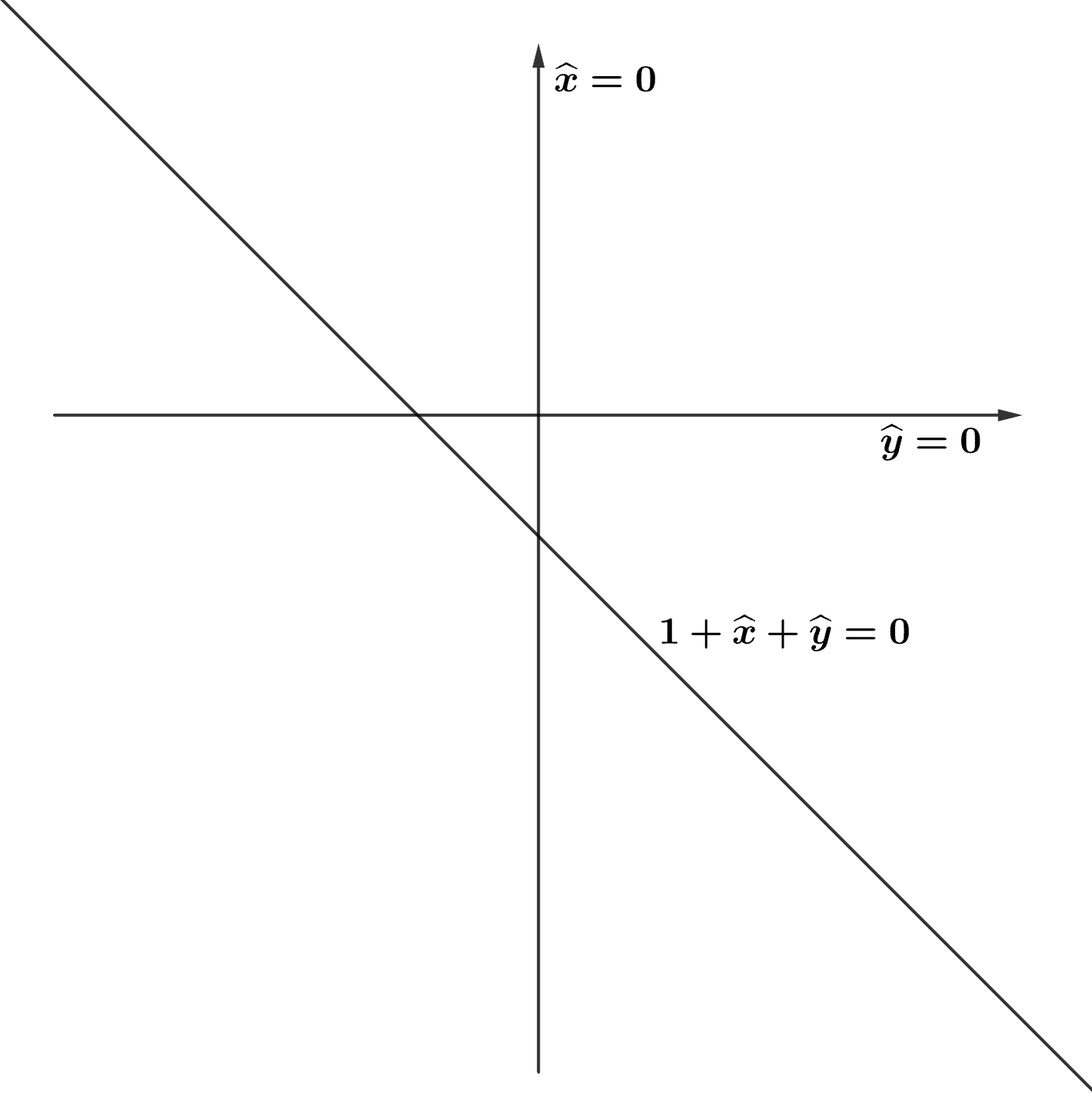
(a) ML degree 1

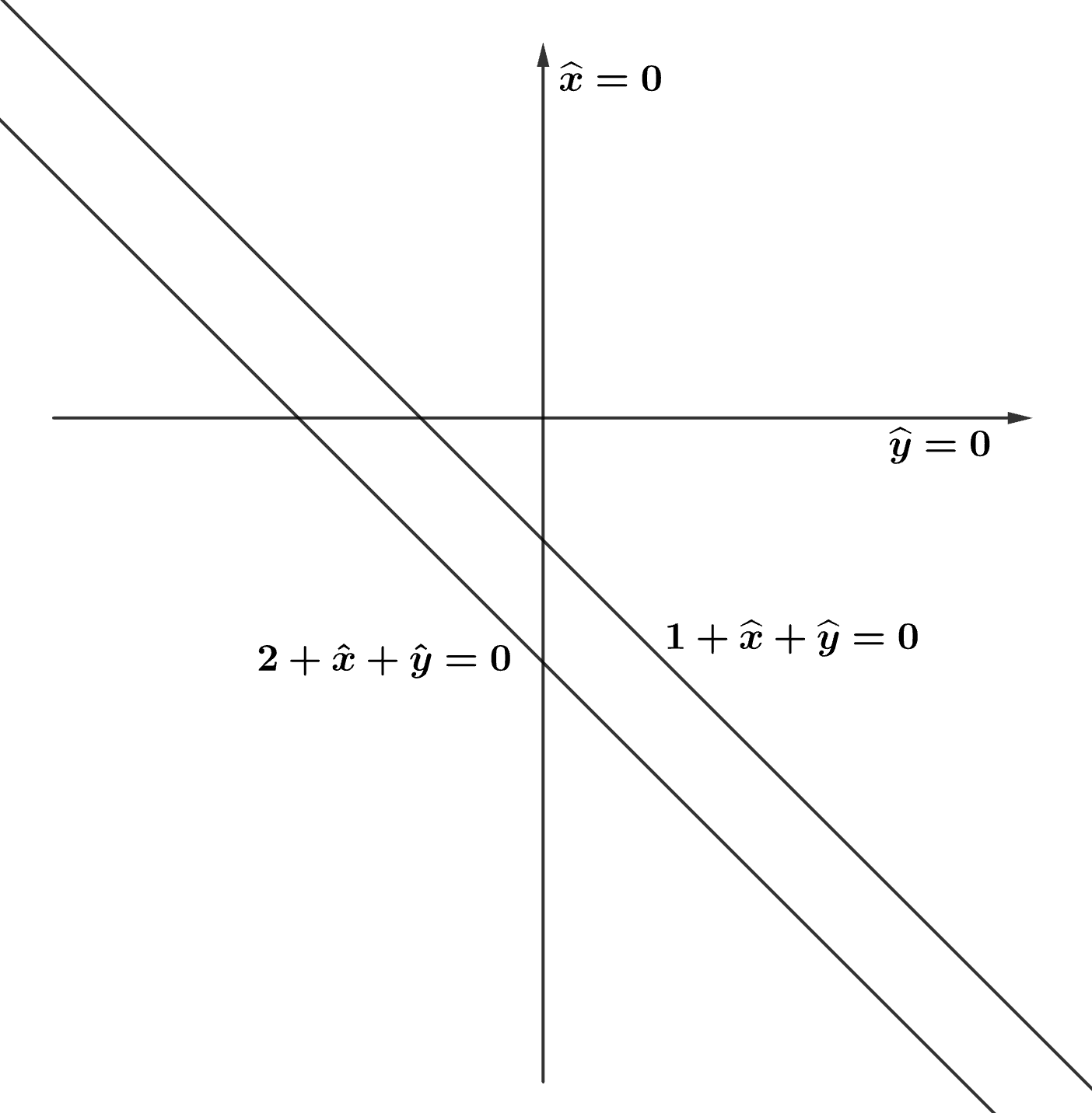
(b) ML degree 2

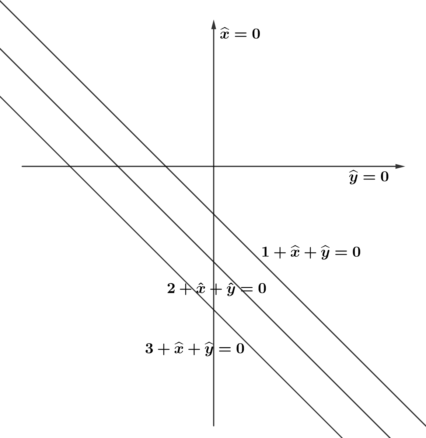
(c) ML degree 3

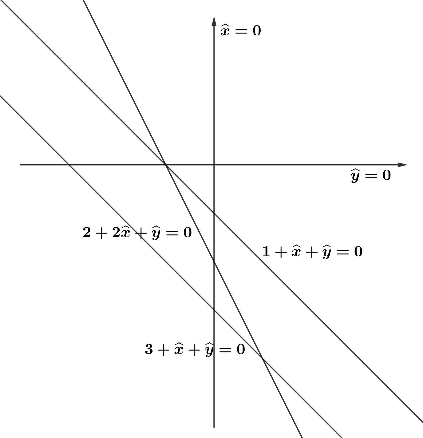
(d) ML degree 4

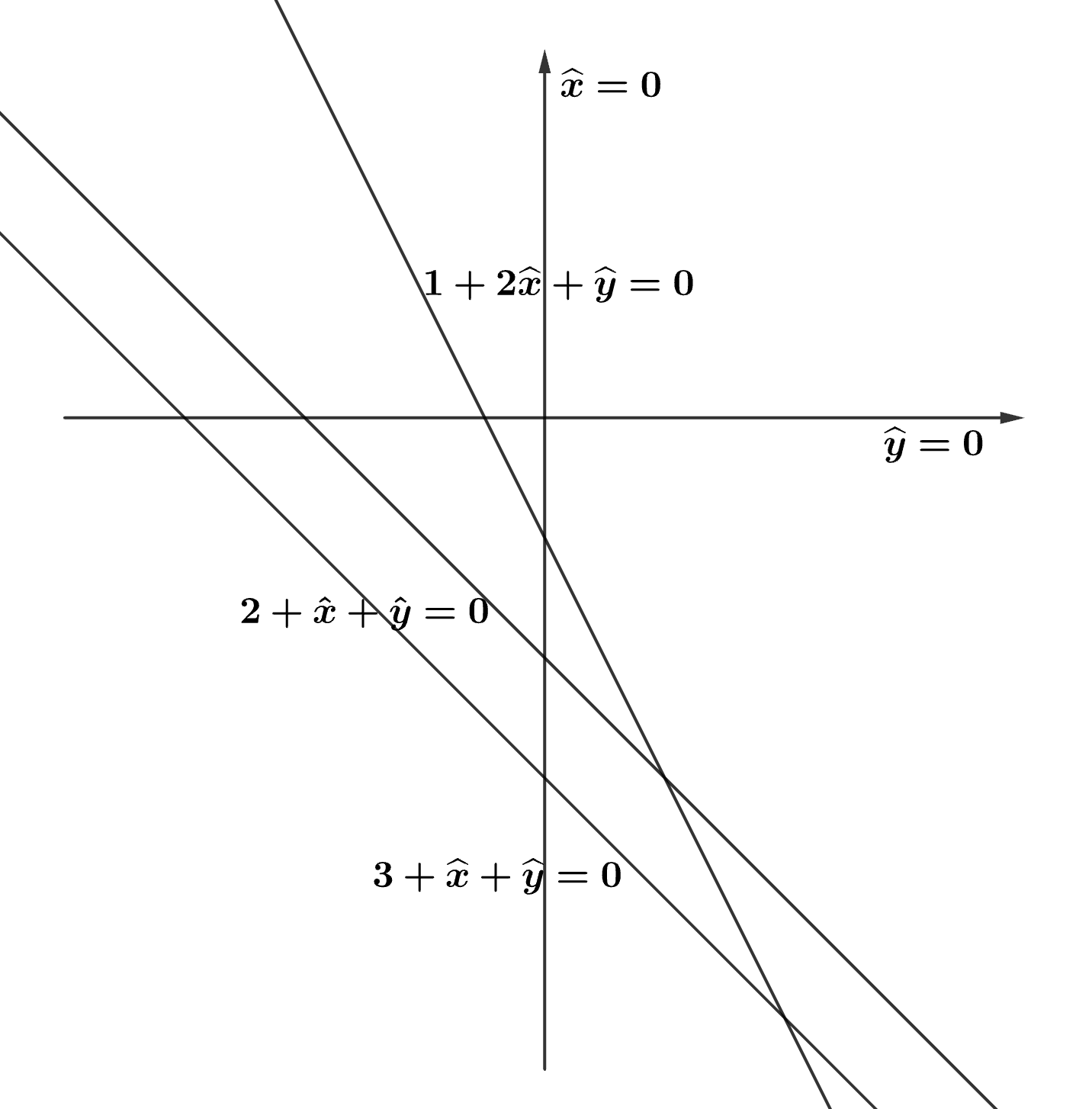
(e) ML degree 5

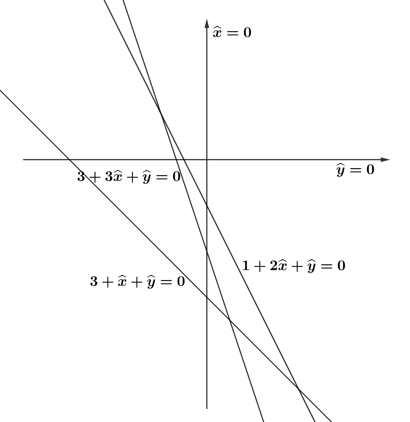
(f) ML degree 6

Figure 2: Hyperplane arrangements for $\mathbb{P}^{2}\times\mathbb{P}^{2}$ realizing all possible ML degrees

Proposition 2.12.

Let $n\geq 3$ and $1\leq k\leq f(n)=\binom{n+1}{2}$. There exist $n$ affine lines $\ell_{i}=0$ in $\mathbb{R}^{2}$ such that

1. no line contains $(0,0)$,

2. no line is parallel to $x=0$ or $y=0$, and

3. the arrangement $\{\ell_{i}=0:\,1\leq i\leq n\}\cup\{x=0\}\cup\{y=0\}$ forms $k$ bounded regions.

Proof.

We prove the following stronger statement by induction. There exist $n$ lines $\ell_{i}=0$ so that together with $\{x=0\}$ and $\{y=0\}$ the arrangement of these $n+2$ lines has $k$ bounded regions where

• no line $\ell_{i}=0$ contains $(0,0)$,

• no line $\ell_{i}=0$ is parallel to $x=0$ or $y=0$,

• for $k\geq f(n)-n$, all $\ell_{i}=0$ are distinct and there exists a point other than $(0,0)$ which is in the intersection of exactly two different lines.

The base case is $n=3$, $f(3)=6$. The arrangements with 1 and 2 bounded regions use coinciding lines. For $3\leq k\leq 6$ consider the arrangements given in Example 2.11, satisfying the induction hypothesis, which proves the base case. Suppose the statement holds for an arrangement of $n$ lines. Notice that $f(n+1)=f(n)+n+1$. Consider $1\leq k\leq f(n+1)$. If $k\leq f(n)-1=f(n+1)-n-2$, we can find an arrangement of $n$ lines with $k$ bounded regions by induction hypothesis, and we draw the last line coinciding with one of the existing ones. If $k=f(n+1)$, we use $n+1$ lines in general position. Now suppose

$$f(n)\leq k\leq f(n+1)-1=f(n)+n.$$

We first construct an arrangement of $n$ distinct lines with $k-n$ bounded regions such that there exist an intersection point other than $(0,0)$ of exactly two lines, $\ell$ and $\ell^{\prime}$. One of the lines can be $x=0$ or $y=0$. Such an arrangement exists by the induction hypothesis since $k-n\geq f(n)-n$. Now we add a new line $\ell_{n+1}$ going through the special intersection point, so that it also intersects all the other lines in different points. The new line has $n+1$ intersection points. Thus, there are $n$ new bounded regions in the arrangement. As a result we have an arrangement of $n+1$ lines with $k$ bounded regions. By genericity, we may assume that the new line is not parallel to the coordinate axes. Since $n\geq 3$, there exists a line $\ell_{r}$ distinct from $\ell$ and $\ell^{\prime}$. By construction, the lines $\ell_{n+1}$ and $\ell_{r}$ intersect at a point that is not contained on any other line. So we have shown that the inductive step holds for $n+1$ lines. ∎

Corollary 2.13.

Let $1\leq k\leq\binom{n+1}{2}$. There exists a scaling matrix $w\in(\mathbb{R}^{*})^{3\times n}$ such that the scaled Segre embedding $X_{w}$ of $\mathbb{P}^{2}\times\mathbb{P}^{n-1}$ has $\operatorname{mldeg}(X_{w})=k$.

Proof.

By Corollary 2.6, the ML degree equals the number of bounded regions in the following arrangement of $n+2$ lines $x=0$, $y=0$ and $\ell_{i}=0$ where $\ell_{i}=w_{1i}+w_{2i}x+w_{i3}y$ for each $i\leq n$. The condition that $w$ has non-zero entries is equivalent to no line $\ell_{i}=0$ being parallel to the axes or passing through the point $(0,0)$. By Proposition 2.12 there is an arrangement with $k$ bounded regions, which gives the desired $w$. ∎

For scaled Segre embeddings of $\mathbb{P}^{3}\times\mathbb{P}^{n-1}$ the matrix $\widehat{w}$ is $4\times(4+n)$. We move the corresponding hyperplane arrangement to the affine patch $(1,\widehat{x},\widehat{y},\widehat{z})$. The result is an arrangement of $n+3$ planes in $\mathbb{R}^{3}$, given by $\widehat{w}_{1i}+\widehat{w}_{2i}\widehat{x}+\widehat{w}_{3i}\widehat{y}+\widehat{w}_{4i}\widehat{z}=0$. The arrangement contains 3 coordinate planes $\widehat{x}=0$, $\widehat{y}=0$, $\widehat{z}=0$. Since $w$ has no zero entries, the planes defined by a column of $w$ intersect each coordinate axis and does not contain the origin.

In the rest of the section, we call a point of intersection of exactly $k$ hyperplanes a $k$-intersection point.

Proposition 2.14.

For any $n\geq 1$ and $1\leq k\leq\binom{n+2}{3}$ there exist $n$ affine planes in $\mathbb{R}^{3}$ such that together with the coordinate planes the resulting arrangement has $k$ bounded regions.

Proof.

We prove this statement by induction. The cases $n=1$ and $2$ are obvious. Let $n\geq 3$. Denote $f(n)=\binom{n+2}{3}$. If $k\leq f(n-1)$ we draw an arrangement of $n-1$ planes with $k$ regions, which exists by induction hypothesis. The last plane will coincide with one of the existing ones. Define the deficiency of the arrangement of $n$ planes to be the difference between $f(n)$ and the actual number of bounded regions in the arrangement. The goal is to determine an algorithm of constructing plane arrangements with deficiencies between $1$ and

$$f(n)-f(n-1)-1=\binom{n+2}{3}-\binom{n+1}{3}-1=\binom{n+1}{2}-1.$$

This follows from Lemma 2.15 below and here we explain the reasoning. If $n$ is even, we can write the maximal needed deficiency as

$$\binom{n+1}{2}-1=\frac{n(n+1)}{2}-1=n\,\frac{n}{2}+\left(\frac{n}{2}-1\right).$$

An arrangement of $\frac{n}{2}$ pairs of parallel planes with ($\frac{n}{2}-1$) 4-intersection points will have the maximal deficiency $\binom{n+1}{2}-1$. This arrangement will have $f(n-1)+1$ bounded regions. For smaller deficiencies $d\leq\binom{n+1}{2}-1$ write $d=qn+r$, where $q\leq\frac{n}{2}$ and $r<n$ and draw the corresponding arrangement obtained from Lemma 2.15. If $n$ is odd, the maximal deficiency is

$$\binom{n+1}{2}-1=n\,\frac{n-1}{2}+(n-1).$$

The arrangement of $\frac{n-1}{2}$ pairs of parallel planes with an extra plane in general position such that there are $(n-1)$ 4-intersection points will have the maximal deficiency. Thus, the number of bounded regions will be $f(n-1)+1$. For smaller deficiencies the same reasoning as above works. ∎

Lemma 2.15.

There exist $n\geq 3$ planes in $\mathbb{R}^{3}$ containing $q\leq\frac{n}{2}$ pairs of parallel planes and $r<n$ 4-intersection points, such that the arrangement obtained from these planes together with the three coordinate planes has deficiency $qn+r$.

Proof.

In our proof when we refer to an arrangement of planes we mean the arrangement obtained from these planes together with the three coordinate planes. First we will show the statement for $r=0$. Consider the following algorithm that gives an arrangement of $n$ planes with $q$ pairs of parallel ones.

• Step 0: Draw $n-q\geq\frac{n}{2}$ planes in general position,

• Repeat the following step $q$ times: Choose a plane without a parallel pair and draw a parallel one.

We may choose the parallel planes so that the arrangement has no 4-intersection points. The goal is to find the difference between the number of bounded regions formed by the arrangement of $n$ planes in general position and the number of bounded regions of the result of the algorithm. To do that, for each $1\leq i\leq q$ we will find the difference between the number of new bounded regions when we add a plane in general position to the arrangement of $(n-q)+i-1$ planes in general position and the number of new regions after step $i$ of the algorithm. Step $i$ draws a new plane which is parallel to one of the existing ones. Consider the lines of intersection of the new plane with existing ones. The arrangement of lines contains $(n-q+2)$ lines in general position and $(i-1)$ lines which are parallel pairs. An arrangement of $(n-q+2)$ lines in general position has $\binom{n-q+1}{2}$ bounded regions. Given an arrangement of $m=(n-q+2+j)$ lines in the plane with $0\leq j<i-1$, the addition of a line that is parallel to exactly one of the $m$ lines introduces exactly $n-q+j$ bounded regions. Hence the number of bounded regions of the line arrangement is

$$\binom{n-q+1}{2}+(n-q)+(n-q+1)+\ldots+(n-q+i-2)=$$

$$(n-q)+\sum_{j=1}^{n-q+i-2}j=-(i-1)+\sum_{j=1}^{n-q+i-1}j=\binom{n-q+i}{2}-(i-1).$$

The number of new bounded regions produced when we add a plane in general position to the arrangement of $(n-q)+i-1$ planes in general position is

$$\binom{n-q+i+1}{2}.$$

Thus the increase of deficiency of step $i$ is

$$\binom{n-q+i+1}{2}-\binom{n-q+i}{2}+(i-1)=n-q+i+(i-1),$$

and the total deficiency is

$$\sum_{i=1}^{q}(n-q+i+(i-1))=nq-q^{2}+\frac{q(q+1)}{2}+\frac{q(q-1)}{2}=nq.$$

For the case $r>0$ we modify the arrangement. Let us fix one of $n$ planes and change the rest of the arrangement in the following way to create $r\leq n-1$ 4-intersection points. The fixed plane creates three 3-intersection points with coordinate planes. We repeat the following process $r$ times. Select a $3$-intersection point $p$ of fixed planes and coordinate planes $p=P_{1}\cap P_{2}\cap P_{3}$ together with a plane $Q$ that has not been fixed, such that $Q$ is not parallel to any of $P_{1}$, $P_{2}$, or $P_{3}$. Translate $Q$ in a direction parallel to its normal so that it passes through $p$, thus creating a 4-intersection point. We then add $Q$ to the set of fixed planes and repeat. By the original construction of the arrangement, the planes $P_{1}$, $P_{2}$, $P_{3}$ and $Q$ are in general position or they are coordinate planes. So the translation introduces exactly one $4$-intersection point. At each of the $r$ steps, we lose exactly one bounded region. Indeed, the number of regions created by a plane is equal to the number of bounded regions of the arrangement of the intersection lines on a plane. Consider this arrangement for $Q$. Before the translation, the arrangement of lines on $Q$ consists of $n-1$ or $n-2$ lines with no 3-intersections. In particular, the number of bounded regions in $Q$ depends only upon the number of pairs of parallel lines. If we translate $Q$ in a direction parallel to its normal, then we introduce no new lines on $Q$ and parallel lines on $Q$ remain parallel. Therefore, by moving $Q$ we create one 4-intersection point, which reduces the number of bounded regions by exactly one. ∎

Corollary 2.16.

Let $1\leq k\leq\binom{n+2}{3}$. There exists a scaling matrix $w\in(\mathbb{R}^{*})^{4\times n}$ such that the scaled Segre embedding $X_{w}$ of $\mathbb{P}^{3}\times\mathbb{P}^{n-1}$ has $\operatorname{mldeg}(X_{w})=k$.

This finishes the proof of Theorem 1.4. The following proposition presents the partial result about the possible ML degrees of scaled Segre embeddings of $\mathbb{P}^{m-1}\times\mathbb{P}^{n-1}$ for $m>4$. It shows that for big enough $n$ it is possible to find scalings realizing ML degrees ranging from a fixed constant up to the degree of the variety.

Proposition 2.17.

Let $d>0$. There exists $n_{0}$ and $k_{0}$, such that for every $n\geq n_{0}$ we can realize an arrangement of $n$ hyperplanes in $\mathbb{R}^{d}$ together with $d$ coordinate hyperplanes such that the number of bounded regions is $k$ for all

$$k_{0}\leq k\leq\binom{n+d-1}{d}.$$

Proof.

Denote the maximum number of bounded regions formed by $n$ hyperplanes and $d$ coordinate hyperplanes by $f_{d}(n)=\binom{n+d-1}{d}$. Consider the following algorithm constructing hyperplane arrangements. Fix an integer $0\leq t\leq n-1$ and a sequence of positive integers $A_{1},\dots,A_{t}$ such that $A_{1}+\dots+A_{t}\leq n-1$.

• Add the first hyperplane in general position,

• For $j$ from $1$ to $t$: draw $A_{j}$ hyperplanes through a $d$-intersection point,

• Draw $n-1-\sum_{j=1}^{t}A_{j}$ hyperplanes in general position.

For instance, if $t=0$, the result is $n$ hyperplanes in general position, which gives $f_{d}(n)$ regions. If $t>0$, the arrangement will have fewer bounded regions. The goal now is to estimate the difference.

Suppose at step $j-1$ there were $M$ hyperplanes together with $d$ coordinate hyperplanes. Define $L(M,j)$ to be the difference between the number of new regions created if we were to add $A_{j}$ hyperplanes in general position and the actual number of new regions created after step $j$. To estimate this difference, consider the $(d+A_{j})$-intersection point after step $j$. If we move each of $A_{j}$ added hyperplanes in a random direction, the $(d+A_{j})$-intersection point will vanish. These $A_{j}$ hyperplanes will be in general position, since there are no other constraints. If the changes are small enough, this will not affect the number of bounded regions formed by the existing hyperplanes. The bounded regions that can appear this way are regions formed by $d+A_{j}$ hyperplanes. Then $L(M,j)$ does not depend on $M$ and

$$L(M,j)=L(j)=\binom{A_{j}+d-1}{d}.$$

We will show that for big enough $n$, the deficiency created by this procedure is $s$ for any $1\leq s\leq f_{d}(n)-f_{d}(n-1)-1$. It will follow that starting from some $n_{0}$ we can construct an arrangement with $n$ hyperplanes with $k$ bounded regions where

$$f_{d}(n-1)+1\leq k\leq f_{d}(n).$$

Define $A(k)$ to be the minimum $n$ such that for every $i$ from $1$ to $k$ the above algorithm can produce an arrangement of $n$ hyperplanes with deficiency $i$. Explicitly, $A(k)$ is given by

$$A(k)=1+\max_{i\leq k}\min_{\{A_{j}\}}\left\{\sum A_{j}\Big{|}\sum\binom{A_{j}+d-1}{d}=i\right\}.$$

For example, $A(1)=2$, since we need at least two hyperplanes to construct an arrangement with deficiency $1$. Moreover, $A(2)$ is also $2$. Now the goal is to show that there exists $n_{0}$, such that for all $n\geq n_{0}$ we have

$$A(f_{d}(n)-f_{d}(n-1)-1)\leq n.$$

Firstly, we can show that $A(f_{d}(n))\leq cn$ for some $c>0$. It holds for every $n>0$ that

$$A(f_{d}(n+1))\leq n+A(f_{d}(n+1)-f_{d}(n)),$$

because given an arrangement with total deficiency $f_{d}(n+1)-f_{d}(n)$, we can draw $n$ more hyperplanes through one point to increase this deficiency by $f_{d}(n)$. Now

$$f_{d}(n+1)-f_{d}(n)=\binom{n+d}{d}-\binom{n+d-1}{d}=\binom{n+d-1}{d-1}\leq f_{d}(m),$$

for $m\geq\sqrt[d]{d(n+d)^{d-1}}$. Indeed,

$$\binom{n+d-1}{d-1}\leq\frac{(n+d)^{d-1}}{(d-1)!}\leq\frac{m^{d}}{d!}\leq\binom{m+d-1}{d}.$$

Thus with $u(n)=A(f_{d}(n))$,

$$u(n+1)\leq n+u\left(\sqrt[d]{d(n+d)^{d-1}}\right).$$

It follows that there exist $c>0$ and $n_{1}$, such that for all $n\geq n_{1}$, $u(n)\leq cn$. Finally, there exist $n_{0}\geq n_{1}$, such that for all $n>n_{0}$

$$A\left(f_{d}(n)-f_{d}(n-1)-1\right)\leq A\left(f_{d}\left(\sqrt[d]{d(n+d)^{d-1}}\right)\right)\leq c\sqrt[d]{d(n+d)^{d-1}}\leq n.$$

Now let $k_{0}=\binom{n_{0}+d-2}{d}+1$. Given $n\geq n_{0}$ and $k\geq k_{0}$, find $n^{\prime}\geq n_{0}$, such that

$$\binom{n^{\prime}+d-2}{d}+1\leq k\leq\binom{n^{\prime}+d-1}{d}$$

and construct the arrangement by the algorithm using $n^{\prime}$ hyperplanes. Then add $n-n^{\prime}$ hyperplanes which coincide with existing ones. ∎

Conjecture 2.18.

Fix $m\geq 4$ and $n\geq m$. For all $k$ such that $1\leq k\leq\binom{n+m-2}{m-1}$, there exist $n$ hyperplanes in $\mathbb{R}^{m-1}$, such that, together with the $m-1$ coordinate hyperplanes, the arrangement of all $m+n-1$ hyperplanes has exactly $k$ bounded regions.

2.3 Computations for $\mathbb{P}^{3}\times\mathbb{P}^{n-1}$

In this section, we compute ML degrees of scaled Segre embeddings of $\mathbb{P}^{3}\times\mathbb{P}^{n-1}$ via beta invariants. Recall Definition 1.2, that $M_{w}$ is the matroid of a scaling $w\in(\mathbb{C}^{*})^{m\times n}$ for $\mathbb{P}^{m-1}\times\mathbb{P}^{n-1}$. Not all matroids arise in this way as $M_{w}$ has the following special property.

Definition 2.19.

We say that a matroid $M$ on $[n]$ is special if there exists a basis $B$ of $M$ such that for all $i\in B$ and for all $j\in[n]\backslash B$ we have $(B\backslash\{i\})\cup\{j\}$ is a basis of $M$. In this case, we say that $B$ is a special basis of $M$.

Proposition 2.20.

For any scaling matrix $w\in(\mathbb{C}^{*})^{m\times n}$ the matroid $M_{w}$ is special.

Proof.

Let $B=\{1,2,\dots,m\}$. The first $m$ columns of $\widehat{w}$ is the identity matrix, hence $B$ is a basis of $M_{w}$. Fix $i\in B$ and $j\in[n+m]\backslash B$. Consider the submatrix $S$ of $\widehat{w}$ given by the columns indexed by $(B\backslash\{i\})\cup\{j\}$. We have $\det(S)=(-1)^{i-1}w_{ij}\neq 0$, and so $(B\backslash\{i\})\cup\{j\}$ is a basis for $M_{w}$. We conclude that $M_{w}$ is special. ∎

Remark 2.21.

We note that the following converse to Proposition 2.20 holds. Suppose that $M$ is a special matroid on $[m+n]$ of rank $m$ that is realizable over $\mathbb{C}$. Then there exists a scaling $w\in(\mathbb{C}^{*})^{m\times n}$ such that $M_{w}\cong M$ are isomorphic.

By Theorem 1.3, the ML degree of the scaled Segre embedding $X_{w}$ of $\mathbb{P}^{3}\times\mathbb{P}^{n-1}$ coincides with the beta invariant of the special matroid $M_{w}$. In the following examples, we compute the beta invariants of all special matroids in the cases where $n$ is $4$ and $5$. These computations are based on an online database of matroids, which, in turn, is based on [AF96]. In general, not all special matroids are realizable over $\mathbb{C}$ and checking realizability is a computationally expensive task. The data-sets used below contain non-realizable matroids. However, since $n$ is small, it is reasonable to assume that the special matroids in the following examples are all realizable over $\mathbb{C}$.

Example 2.22 ($n=4$).

Up to isomorphism, there are $940$ matroids of rank $4$ on $8$ elements, of which $568$ are special. The beta invariants of these special matroids are tallied in Table 2. In particular, all ML degrees between $1$ and $20$ are attained.

Example 2.23 ($n=5$).

There are $190\,214$ matroids of rank $4$ on $9$ elements up to isomorphism with $185\,253$ special matroids. Their beta invariants are tallied in Table 3. In particular, all possible ML degrees between $1$ and $35$ are attained. We observe that only a small proportion of all matroids are not special and the distribution of the number of matroids with a particular beta invariant is unimodal.

Notice that in both examples above the number of matroids realizing the maximum ML degree $\binom{n+m-2}{m-1}$ is one. The reason is clear if we look at an affine patch of the matroid hyperplane arrangement, because the only possible arrangement with the same number of bounded regions is a set of $n$ hyperplanes in $\mathbb{R}^{m-1}$ in general position. The same holds for ML degree $\binom{n+m-2}{m-1}-1$. In this case, the arrangement must have exactly one $(m+1)$-intersection point and, up to isomorphism, there is only one way to achieve this.

Beta invariant	1	2	3	4	5	6	7	8	9	10
No. matroids	1	6	10	16	17	26	27	33	29	47
Beta invariant	11	12	13	14	15	16	17	18	19	20
No. matroids	59	74	84	67	40	20	7	3	1	1

Table 2: The beta invariants of all $568$ special matroids of rank $4$ on $[8]$.

Beta invariant	1	2	3	4	5	6	7	8	9
No. matroids	1	9	20	34	48	75	93	133	168
Beta invariant	10	11	12	13	14	15	16	17	18
No. matroids	265	361	486	636	760	845	1180	1827	2881
Beta invariant	19	20	21	22	23	24	25	26	27
No. matroids	4767	7807	11600	17153	25328	33480	33963	24293	11856
Beta invariant	28	29	30	31	32	33	34	35
No. matroids	3961	967	199	42	10	3	1	1

Table 3: The beta invariants of all $185\,253$ special matroids of rank $4$ on $[9]$.

Remark 2.24.

Without a significant theoretical improvement, it does not seem possible to compute the beta invariants of all special matroids in the case where $n=6$. There are $4\,886\,380\,924$ matroids of rank $4$ on $10$ elements and, similarly to the $n=5$ example, we expect that a large proportion of these are special.

2.4 The principal $A$-determinant of $\mathbb{P}^{1}\times\mathbb{P}^{1}\times\mathbb{P}^{n-1}$

In this section we determine the principal $A$-determinant of the Segre embedding $\mathbb{P}^{1}\times\mathbb{P}^{1}\times\mathbb{P}^{n-1}$ and investigate the ML degrees under certain scalings. The polytope $P_{n}\subset\mathbb{R}^{2}\oplus\mathbb{R}^{2}\oplus\mathbb{R}^{n}$ of $\mathbb{P}^{1}\times\mathbb{P}^{1}\times\mathbb{P}^{n-1}$ is the convex hull of $e_{i}\oplus e_{j}\oplus f_{k}$ for each $i,j\in[2]$ and $k\in[n]$. Here $e_{i}$ and $f_{k}$ are the standard unit vectors of $\mathbb{R}^{2}$ and $\mathbb{R}^{n}$, respectively. The polytope $P_{n}$ is the product of standard simplices $\Delta_{1}\times\Delta_{1}\times\Delta_{n-1}$ and it is the set of points $x\oplus y\oplus z$ defined by the following equations and inequalities:

$$x_{1}+x_{2}=1,\,0\leq x_{i}\leq 1,\quad y_{1}+y_{2}=1,\,0\leq y_{j}\leq 1,\quad z_{1}+\dots+z_{n}=1,\,0\leq z_{k}\leq 1$$

for all $i,j\in[2]$ and $k\in[n]$.

Proposition 2.25.

Up to an affine unimodular transformation, $P_{n}=\Delta_{1}\times\Delta_{1}\times\Delta_{n-1}$ has two kinds of non-simplicial proper faces. There are $2\binom{n}{k}$ faces equal to $P_{k}$ for each $k\in[n-1]$. All others are equal to $\Delta_{1}\times\Delta_{k}$ for some $k\in[n-1]$.

Proof.

This follows from the formulation of $P_{n}$ by inequalities. The facets of $P_{n}$ are supported by the hyperplanes defined by $x_{i}=0$, $y_{i}=0$, and $z_{j}=0$ for each $i\in[2]$ and $j\in[n]$. If the facet is defined by $z_{j}=0$, then it is equal to $P_{n-1}$. Otherwise, if the facet is defined by either $x_{i}=0$ or $y_{i}=0$, then it is equal to $\Delta_{1}\times\Delta_{n-1}$. ∎

The only faces of $P_{n}$ for which we require a novel description of the $A$-discriminant are those faces of the form $P_{k}$ for each $k\in[n]$. In this case, the $A$-discriminant is known as a hyperdeterminant of format $2\times 2\times k$. For further details see [GKZ94, Chapter 14].

Proposition 2.26 ([GKZ94, Chapter 14, Theorem 1.3]).

The $A$-discriminant for $P_{n}$ is non-trivial if and only if $n=2$ or $n=3$. In these cases, the $A$-discriminant is the hyperdeterminant for the $2\times 2\times 2$ and $2\times 2\times 3$ tensors, respectively.

In the following examples, we give an explicit description of these hyperdeterminants.

Example 2.27.

The $2\times 2\times 2$ hyperdeterminant, often called Cayley’s hyperdeterminant after the approach taken in [Cay45], is the $A$-discriminant associated to the matrix

$$A=\begin{pmatrix}1&1&1&1&0&0&0&0\\ 1&1&0&0&1&1&0&0\\ 1&0&1&0&1&0&1&0\\ 0&1&0&1&0&1&0&1\end{pmatrix},$$

which is

$$w_{4}^{2}w_{5}^{2}+w_{3}^{2}w_{6}^{2}+w_{2}^{2}w_{7}^{2}+w_{1}^{2}w_{8}^{2}-2w_{3}w_{4}w_{5}w_{6}-2w_{2}w_{4}w_{5}w_{7}-2w_{2}w_{3}w_{6}w_{7}$$

$$-2w_{1}w_{4}w_{5}w_{8}-2w_{1}w_{3}w_{6}w_{8}-2w_{1}w_{2}w_{7}w_{8}+4w_{1}w_{4}w_{6}w_{7}+4w_{2}w_{3}w_{5}w_{8}.$$

Example 2.28.

The $2\times 2\times 3$ hyperdeterminant is the $A$-discriminant associated to the matrix

$$A=\setcounter{MaxMatrixCols}{12}\begin{pmatrix}1&1&1&1&0&0&0&0&0&0&0&0\\ 0&0&0&0&1&1&1&1&0&0&0&0\\ 1&1&0&0&1&1&0&0&1&1&0&0\\ 1&0&1&0&1&0&1&0&1&0&1&0\\ 0&1&0&1&0&1&0&1&0&1&0&1\end{pmatrix},$$

which is given by the polynomial

$$w_{4}^{2}w_{6}w_{7}w_{9}^{2}-w_{3}w_{4}w_{6}w_{8}w_{9}^{2}-w_{2}w_{4}w_{7}w_{8}w_{9}^{2}+w_{2}w_{3}w_{8}^{2}w_{9}^{2}-w_{4}^{2}w_{5}w_{7}w_{9}w_{10}$$

$$-w_{3}w_{4}w_{6}w_{7}w_{9}w_{10}+w_{2}w_{4}w_{7}^{2}w_{9}w_{10}+w_{3}w_{4}w_{5}w_{8}w_{9}w_{10}+w_{3}^{2}w_{6}w_{8}w_{9}w_{10}$$

$$-w_{2}w_{3}w_{7}w_{8}w_{9}w_{10}+w_{1}w_{4}w_{7}w_{8}w_{9}w_{10}-w_{1}w_{3}w_{8}^{2}w_{9}w_{10}+w_{3}w_{4}w_{5}w_{7}w_{10}^{2}$$

$$-w_{1}w_{4}w_{7}^{2}w_{10}^{2}-w_{3}^{2}w_{5}w_{8}w_{10}^{2}+w_{1}w_{3}w_{7}w_{8}w_{10}^{2}-w_{4}^{2}w_{5}w_{6}w_{9}w_{11}+w_{3}w_{4}w_{6}^{2}w_{9}w_{11}$$

$$-w_{2}w_{4}w_{6}w_{7}w_{9}w_{11}+w_{2}w_{4}w_{5}w_{8}w_{9}w_{11}-w_{2}w_{3}w_{6}w_{8}w_{9}w_{11}+w_{1}w_{4}w_{6}w_{8}w_{9}w_{11}$$

$$+w_{2}^{2}w_{7}w_{8}w_{9}w_{11}-w_{1}w_{2}w_{8}^{2}w_{9}w_{11}+w_{4}^{2}w_{5}^{2}w_{10}w_{11}-w_{3}w_{4}w_{5}w_{6}w_{10}w_{11}$$

$$-w_{2}w_{4}w_{5}w_{7}w_{10}w_{11}+2w_{1}w_{4}w_{6}w_{7}w_{10}w_{11}+2w_{2}w_{3}w_{5}w_{8}w_{10}w_{11}-2w_{1}w_{4}w_{5}w_{8}w_{10}w_{11}$$

$$-w_{1}w_{3}w_{6}w_{8}w_{10}w_{11}-w_{1}w_{2}w_{7}w_{8}w_{10}w_{11}+w_{1}^{2}w_{8}^{2}w_{10}w_{11}+w_{2}w_{4}w_{5}w_{6}w_{11}^{2}$$

$$-w_{1}w_{4}w_{6}^{2}w_{11}^{2}-w_{2}^{2}w_{5}w_{8}w_{11}^{2}+w_{1}w_{2}w_{6}w_{8}w_{11}^{2}+w_{3}w_{4}w_{5}w_{6}w_{9}w_{12}-w_{3}^{2}w_{6}^{2}w_{9}w_{12}$$

$$+w_{2}w_{4}w_{5}w_{7}w_{9}w_{12}+2w_{2}w_{3}w_{6}w_{7}w_{9}w_{12}-2w_{1}w_{4}w_{6}w_{7}w_{9}w_{12}-w_{2}^{2}w_{7}^{2}w_{9}w_{12}$$

$$-2w_{2}w_{3}w_{5}w_{8}w_{9}w_{12}+w_{1}w_{3}w_{6}w_{8}w_{9}w_{12}+w_{1}w_{2}w_{7}w_{8}w_{9}w_{12}-w_{3}w_{4}w_{5}^{2}w_{10}w_{12}$$

$$+w_{3}^{2}w_{5}w_{6}w_{10}w_{12}-w_{2}w_{3}w_{5}w_{7}w_{10}w_{12}+w_{1}w_{4}w_{5}w_{7}w_{10}w_{12}-w_{1}w_{3}w_{6}w_{7}w_{10}w_{12}$$

$$+w_{1}w_{2}w_{7}^{2}w_{10}w_{12}+w_{1}w_{3}w_{5}w_{8}w_{10}w_{12}-w_{1}^{2}w_{7}w_{8}w_{10}w_{12}-w_{2}w_{4}w_{5}^{2}w_{11}w_{12}$$

$$-w_{2}w_{3}w_{5}w_{6}w_{11}w_{12}+w_{1}w_{4}w_{5}w_{6}w_{11}w_{12}+w_{1}w_{3}w_{6}^{2}w_{11}w_{12}+w_{2}^{2}w_{5}w_{7}w_{11}w_{12}$$

$$-w_{1}w_{2}w_{6}w_{7}w_{11}w_{12}+w_{1}w_{2}w_{5}w_{8}w_{11}w_{12}-w_{1}^{2}w_{6}w_{8}w_{11}w_{12}+w_{2}w_{3}w_{5}^{2}w_{12}^{2}$$

$$-w_{1}w_{3}w_{5}w_{6}w_{12}^{2}-w_{1}w_{2}w_{5}w_{7}w_{12}^{2}+w_{1}^{2}w_{6}w_{7}w_{12}^{2}.$$

Proof of Theorem 1.5.

Proposition 2.25 classifies all non-simplical faces of $\Delta_{1}\times\Delta_{1}\times\Delta_{n-1}$. The factors of the principal $A$-determinant come from these faces. Out of the two types of faces identified in the same proposition, the first type contributes either $2\times 2\times 2$ hyperdeterminants or $2\times 2\times 3$ hyperdeterminants of the $2\times 2\times n$ tensor $w$ by Proposition 2.26 The second type of face contributes the $2$-minors of all slices of $w$. ∎

Recall from Theorem 1.3 that the ML degree of $\mathbb{P}^{m-1}\times\mathbb{P}^{n-1}$ with respect to a scaling $w$ is determined precisely by which factors of the principal $A$-determinant vanish. We conjecture that the same is true for $\mathbb{P}^{1}\times\mathbb{P}^{1}\times\mathbb{P}^{n-1}$.

Conjecture 2.29.

Let $w$ and $w^{\prime}$ be scalings for $\mathbb{P}^{1}\times\mathbb{P}^{1}\times\mathbb{P}^{n}$ such that for any face $\Gamma\subseteq P_{n}$ we have $\Delta_{\Gamma}(w)=0$ if and only if $\Delta_{\Gamma}(w^{\prime})=0$. Then $\operatorname{mldeg}(X_{w})=\operatorname{mldeg}(X_{w^{\prime}})$.

Also, as in the case of $\mathbb{P}^{m-1}\times\mathbb{P}^{n-1}$, the vanishing of certain factors of the principal $A$-determinant $E_{A}$ forces other factors to vanish as well. Below we give two such cases. Then we return to the question of the possible ML degrees attained as $w$ varies. To keep track of the determinants and hyperdeterminants of $w$, we introduce the following notation: For each subset $K\in\binom{[n]}{2}$ or $K\in\binom{[n]}{3}$, we write $D_{K}$ for the $2\times 2\times 2$ and $2\times 2\times 3$ hyperdeterminant of $(w_{ijk})_{k\in K}$.

Definition 2.30.

Let $U=\{U_{1},U_{2},U_{3}\}$ be a set of three distinct $2$-minors of slices of $w$. We say that $U$ is a square cup if each of the following hold:

• There is a $2\times 2\times 2$ sub-tensor of $w$ containing $U_{1}$, $U_{2}$, and $U_{3}$,

• The minors $U_{1}$ and $U_{2}$ have disjoint sets of variables.

Proposition 2.31.

Let $w=(w_{ijk})\in(\mathbb{C}^{*})^{2\times 2\times 2}$. If there exists a square cup $U$ such that each $2$-minor of $U$ vanishes on $w$, then the hyperdeterminant of $w$ vanishes.

Proof.

Let $I=\langle U_{1},U_{2},U_{3}\rangle\subseteq\mathbb{C}[w_{ijk}]$ be the ideal generated by the square cup. Let $J=(I:(\prod_{i,j,k}w_{ijk})^{\infty})$ be the saturation of $I$ by the product of variables. By a straightforward computation in Macaulay2 [GS], the ideal $J$ is minimally generated by all six $2$-minors of $w$ and contains the hyperdeterminant of $w$. ∎

Proposition 2.32.

Let $w=(w_{ijk})\in(\mathbb{C}^{*})^{2\times 2\times 3}$. If one of the hyperdeterminants $D_{12}$, $D_{13}$, or $D_{23}$ vanishes then so does the hyperdeterminant $D_{123}$. Also, if there exists a pair of vanishing $2$-minors contained in a $1\times 2\times 3$ slice of $w$, then the hyperdeterminant $D_{123}$ vanishes.

Proof.

The proof follows from a direct computation of the saturation of the ideal generated by a hyperdeterminant or the ideal generated by the $2$-minors with respect to the product of the variables. ∎

Example 2.33.

We show that for the scaled Segre embedding of $\mathbb{P}^{1}\times\mathbb{P}^{1}\times\mathbb{P}^{2}$ all possible ML degrees $1,2,\dots,12$ are achieved. Let $A$ be the matrix defining $X$, which is given by

$$A=\setcounter{MaxMatrixCols}{12}\begin{pmatrix}1&1&1&1&0&0&0&0&0&0&0&0\\ 0&0&0&0&1&1&1&1&0&0&0&0\\ 1&1&0&0&1&1&0&0&1&1&0&0\\ 1&0&1&0&1&0&1&0&1&0&1&0\\ 0&1&0&1&0&1&0&1&0&1&0&1\end{pmatrix}.$$

Table 4 shows an example of a scaling of $X_{A}$ that achieves each possible ML degree.

Scaling $w$	ML degree
$(1,1,1,1,\ 1,1,1,1,\ 1,1,1,1)$	$1$
$(1,1,1,1,\ 1,1,1,1,\ 1,1,2,2)$	$2$
$(1,1,1,1,\ 1,1,1,1,\ 1,1,1,2)$	$3$
$(1,1,1,1,\ 1,1,1,1,\ 1,1,2,3)$	$4$
$(1,1,1,1,\ 1,1,1,1,\ 1,2,2,1)$	$5$
$(1,1,1,1,\ 1,1,1,2,\ 1,2,1,1)$	$6$
$(1,1,1,1,\ 1,1,1,2,\ 1,2,3,4)$	$7$
$(1,1,1,1,\ 1,1,1,2,\ 1,2,2,3)$	$8$
$(1,1,1,1,\ 1,1,1,2,\ 1,2,2,5)$	$9$
$(1,1,1,2,\ 1,2,1,3,\ 1,3,2,5)$	$10$
$(1,1,1,2,\ 1,3,2,5,\ 2,3,6,9)$	$11$
$(1,1,1,2,\ 1,3,2,5,\ 1,6,3,7)$	$12$

Table 4: ML degrees of the Segre embedding of $\mathbb{P}^{1}\times\mathbb{P}^{1}\times\mathbb{P}^{2}$ for different scalings.

The following result gives a large family of scalings $w$ for which the corresponding variety has ML degree one.

Proposition 2.34.

Let $X_{w}$ be a scaled Segre embedding of $\mathbb{P}^{1}\times\mathbb{P}^{1}\times\mathbb{P}^{n-1}$ with the scaling $w\in(\mathbb{C}^{*})^{2\times 2\times n}$. If there is a partition of $w=(w_{ijk})$ into parallel slices such that $w$ is constant on each slice, then $X_{w}=X_{A}$. In particular, $X_{A,w}$ has ML degree one.

Proof.

The defining ideal $I_{A}$ of $X_{A}$ is generated by the binomials

$$x_{ijk}x_{i^{\prime}j^{\prime}k^{\prime}}-x_{ijk^{\prime}}x_{i^{\prime}j^{\prime}k},\quad x_{ijk}x_{i^{\prime}j^{\prime}k^{\prime}}-x_{ij^{\prime}k}x_{i^{\prime}jk^{\prime}},\quad x_{ijk}x_{i^{\prime}j^{\prime}k^{\prime}}-x_{ij^{\prime}k^{\prime}}x_{i^{\prime}jk}$$

for all $i,j,i^{\prime},j^{\prime}\in[2]$ and $k,k^{\prime}\in[n]$. Fix a scaling $w$ such that parallel slices of $w$ are constant. Notice that each binomial above is contained in at most two parallel slices of the tensor $X=(x_{ijk})$. If the binomial is contained in a single slice where $w$ is constant then the same generator appears in the analogous generating set for $I_{A,w}$. Suppose that a binomial is contained in two parallel slices. The corresponding generator of the ideal $I_{A,w}$ is obtained by scaling each variable by its corresponding entry in $w$. Since $w$ is constant on each slice, each term of the binomial is scaled by the same factor. Hence the binomial itself is a generator of the ideal $I_{A,w}$. We conclude that the ideals $I_{A}$ and $I_{A,w}$ have the same generating set. ∎

We finish this section by proving that the small-valued ML degrees can always be obtained by an extension of Theorem 1.4 for $\mathbb{P}^{m-1}\times\mathbb{P}^{n-1}$.

Proposition 2.35.

Let $m$ be equal to $2,3$ or $4$. Then for each $1\leq k\leq\binom{n+m-2}{m-1}$ there exists a scaling matrix $w\in(\mathbb{R}^{*})^{l\times m\times n}$ such that $\operatorname{mldeg}(X_{w})=k$ for the scaled Segre embedding $X_{w}$ of $\mathbb{P}^{l-1}\times\mathbb{P}^{m-1}\times\mathbb{P}^{n-1}$.

Proof.

According to Theorem 1.4, for $1\leq k\leq\binom{n+m-2}{m-1}$ there exists a scaling matrix $w^{\prime}=(w_{st}^{\prime})\in(\mathbb{R}^{*})^{m\times n}$ such that $\operatorname{mldeg}(X_{w^{\prime}})=k$, where $X_{w^{\prime}}$ denotes the scaled Segre embedding of $\mathbb{P}^{m-1}\times\mathbb{P}^{n-1}$. Now consider $X_{w}$ with the repeating scaling $w_{ist}=w_{st}^{\prime}$ for all $i\in[l]$. Then $X_{w}$ is the toric fiber product of $\mathbb{P}^{l-1}$ with $X_{w^{\prime}}$ since the chosen scaling $w_{ist}$ can be written as a product $1\cdot w_{st}$. In this case, the ML degree is multiplicative, see e.g. [AKK20, Theorem 5.5] and [AO23, Section 5]. Therefore,

$$\operatorname{mldeg}(X_{w})=\operatorname{mldeg}(\mathbb{P}^{l-1})\cdot\operatorname{mldeg}(X_{w^{\prime}})=1\cdot k=k.\qed$$

Corollary 2.36.

Fix $d\leq n$. The scaled Segre embedding of $\mathbb{P}^{1}\times\mathbb{P}^{1}\times\mathbb{P}^{n-1}$ has ML degree $d$ where the scaling $w=(w_{ijk})$ is given by

$$w_{ijk}=\begin{cases}1&\text{if }k>d\text{ or }i=1,\\ k&\text{if }k\leq d\text{ and }i=2.\end{cases}$$

3 Second Hypersimplex

The focus of this section is on uniform matroids of rank two and their ML degree stratification. The uniform matroid of rank $k$, denoted $U_{d}^{k}$, is the matroid with bases $\binom{[d]}{k}$. Its matroid polytope is the hypersimplex $\Delta_{k,d}$, a $(d-1)$-dimensional polytope with $\binom{d}{k}$ vertices embedded in the $d$-dimensional space.

Example 3.1 (Octahedron).

The uniform matroid $U_{4}^{2}$ of rank two on four elements has bases

$$12,\,13,\,14,\,23,\,24,\,34.$$

Its matroid polytope $\Delta_{2,4}$ shown in Figure 3 is the convex hull of the columns of

$$A=\begin{pmatrix}1&1&1&0&0&0\\ 1&0&0&1&1&0\\ 0&1&0&1&0&1\\ 0&0&1&0&1&1\\ \end{pmatrix}.$$

Figure 3: Matroid polytope of $U_{4}^{2}$.

The ML degree of the scaled toric variety $X_{2,d}^{w}$ corresponding to the second hypersimplex $\Delta_{2,d}$ is bounded above by the degree of the same variety.

Proposition 3.2.

Let $X_{2,d}$ be the toric variety associated to the second hypersimplex $\Delta_{2,d}$. Then

$$\textup{deg}(X_{2,d})=2^{d-1}-d.$$

Proof.

The normalized volume of the hypersimplex $\Delta_{k,d}$ is given by the Eulerian number $A(d-1,k-1)$ [Lap86]. It is well known that $A(d-1,1)=2^{d-1}-d$. ∎

For a better understanding of the achievable ML degrees of $X_{2,d}^{w}$, we present a compact description of the principal $A$-determinant. The lattice points contained in $\Delta_{2,d}$ are $e_{i}+e_{j}$ for $1\leq i<j\leq d$ where $e_{i}$ is the $i$th standard unit vector in $\mathbb{R}^{d}$. These lattice points comprise the columns of the $d\times\binom{d}{2}$ matrix $A$. We assign the scaling constant $w_{ij}$ to each of these lattice points. With this, let $W$ be the following $d\times d$ symmetric matrix with entries

$$W_{ij}=\begin{cases}w_{ij},&i<j,\\ 0,&i=j.\end{cases}$$

Proposition 3.3.

The $A$-discriminant $\Delta(U_{d}^{2})$ of the second hypersimplex $\Delta_{2,d}$ is $\det(W)$.

Proof.

Let $f=\sum_{i<j}w_{ij}\theta_{i}\theta_{j}$ be the polynomial defined by $\Delta_{2,d}$ and the scaling $w$. Since $f$ is homogeneous of degree two, the partial derivatives give a system of linear equations

$$\frac{\partial f}{\partial\theta_{k}}=\sum_{i=1}^{k-1}w_{ik}\theta_{i}+\sum_{j=k+1}^{d}w_{kj}\theta_{j}=0,\quad k\in[d],$$

which is precisely $W\theta=0$. The system has a non-zero solution if and only if $\det(W)=0$. Hence, $\Delta(U^{2}_{d})=\det(W)$. ∎

Corollary 3.4.

The $A$-discriminant $\Delta(U^{2}_{d})$ is homogeneous with respect to the multigrading given by the columns of the matrix $A$ with degree $(2,2,\dots,2)^{T}$.

Proof.

Every term of the determinant $\det(W)$ is of the form $m_{\sigma}=W_{1\sigma(1)}W_{2\sigma(2)}\dots W_{d\sigma(d)}$ for some permutation $\sigma\in\operatorname{Sym}(d)$. Each non-zero entry $W_{ij}$ is a variable with degree $e_{i}+e_{j}$. Therefore, $\textup{deg}(m_{\sigma})=\sum_{i}(e_{i}+e_{\sigma(i)})=2\sum_{i}e_{i}$. ∎

Example 3.5.

Consider the uniform matroid $U_{5}^{2}$. According to Proposition 3.3, the $A$-discriminant is

$$\Delta(U^{2}_{5})=\det\begin{pmatrix}0&w_{12}&w_{13}&w_{14}&w_{15}\\ w_{12}&0&w_{23}&w_{24}&w_{25}\\ w_{13}&w_{23}&0&w_{34}&w_{35}\\ w_{14}&w_{24}&w_{34}&0&w_{45}\\ w_{15}&w_{25}&w_{35}&w_{45}&0\\ \end{pmatrix}$$

$$=w_{14}w_{15}w_{23}w_{25}w_{34}+w_{13}w_{15}w_{24}w_{25}w_{34}+w_{14}w_{15}w_{23}w_{24}w_{35}+w_{13}w_{14}w_{24}w_{25}w_{35}$$

$$+w_{12}w_{15}w_{24}w_{34}w_{35}+w_{12}w_{14}w_{25}w_{34}w_{35}+w_{13}w_{15}w_{23}w_{24}w_{45}+w_{13}w_{14}w_{23}w_{25}w_{45}$$

$$+w_{12}w_{15}w_{23}w_{34}w_{45}+w_{12}w_{13}w_{25}w_{34}w_{45}+w_{12}w_{14}w_{23}w_{35}w_{45}+w_{12}w_{13}w_{24}w_{35}w_{45}$$

$$-w_{15}^{2}w_{23}w_{24}w_{34}-w_{13}w_{14}w_{25}^{2}w_{34}-w_{12}w_{15}w_{25}w_{34}^{2}-w_{13}w_{15}w_{24}^{2}w_{35}-w_{14}^{2}w_{23}w_{25}w_{35}$$

$$-w_{12}w_{14}w_{24}w_{35}^{2}-w_{14}w_{15}w_{23}^{2}w_{45}-w_{13}^{2}w_{24}w_{25}w_{45}-w_{12}^{2}w_{34}w_{35}w_{45}-w_{12}w_{13}w_{23}w_{45}^{2}.$$

We are now ready to present the principal $A$-determinant of the second hypersimplex. For every subset $E\subset[d]$ with $|E|\geq 2$, we denote the uniform matroid of rank two on the ground set $E$ by $U_{E}^{2}$.

Theorem 3.6.

The principal $A$-determinant of the second hypersimplex $\Delta_{2,d}$ for $d\geq 4$ is

$$\prod_{\begin{subarray}{c}E\subseteq[d]\\ |E|\geq 4\end{subarray}}\Delta(U^{2}_{E}).$$

In particular, the only faces of $\Delta_{2,d}$ that contribute non-unit factors to this principal $A$-determinant arise from matroid deletion.

Proof.

The hypersimplex $\Delta_{2,d}$ has the half-space description

$$\Delta_{2,d}=\{x\in\mathbb{R}^{d}\colon 0\leq x_{i}\leq 1\text{ for all }i\in[d]\text{ and }x_{1}+x_{2}+\dots+x_{d}=2\}.$$

Therefore, the facets of $\Delta_{2,d}$ are defined by the hyperplanes $x_{i}=0$ and $x_{i}=1$ for each $i\in[d]$. In particular, $\Delta_{2,d}$ has $d$ facets of the form $\Delta_{2,d}\cap\{x_{i}=0\}$, which are unimodularly equivalent to $\Delta_{2,d-1}$. These facets are the matroid polytopes of $U^{2}_{E}$ with $E=[d]\backslash\{i\}$. The other $d$ facets of the form $\Delta_{2,d}\cap\{x_{i}=1\}$ are unimodular simplices of dimension $d-1$ (see e.g. [Bor08]).

By induction on $d$, the faces of $\Delta_{2,d}$ are the matroid polytopes of $U^{2}_{E}$ with $E\subseteq[d]$ or unimodular simplices. Each simplicial face contributes a trivial factor to the principal $A$-determinant. In particular, the matroid polytopes of $U^{2}_{2}$ and $U^{2}_{3}$ are unimodular simplices. So the non-simplicial faces of $\Delta_{2,d}$ are the matroid polytopes of $U^{2}_{E}$ for each $E\subseteq[d]$ with $|E|\geq 4$. ∎

As in the previous section we want to understand which ML degrees can be achieved by choosing different scalings. The singularities of the polynomials defined by the faces of the underlying polytope can help with this goal (see e.g. [AKK20, Example 4.4]).

Proposition 3.7.

Let $\Gamma_{3}$ be a three-dimensional face of $\Delta_{2,d}$. Then $f_{w}$ defined by $\Gamma_{3}$ has at most one singularity.

Proof.

We take $\Gamma_{3}$ to be $\Delta_{2,4}$, and after an affine unimodular transformation we can remove the first coordinate of each vertex of $\Delta_{2,4}$ to get a full-dimensional polytope in $\mathbb{R}^{3}$. Each lattice point of this polytope has at most two non-zero entries. Therefore,

$$\frac{\partial f_{w}}{\partial\theta_{i}}(\theta)=0,\quad 1\leq i\leq 3,$$

can be written as a system of linear equations $W\theta=b$. Since $\textup{det}(W)=2w_{12}w_{13}w_{23}\neq 0$, there is a unique solution for $\theta$ in $w_{ij}$. Substitution of $\theta$ in $f_{w}$ yields $f_{w}=0$ or $f_{w}\neq 0$. ∎

Corollary 3.8.

Let $w$ be a scaling such that $k$ factors of the principal $A$-determinant of the second hypersimplex $\Delta_{2,d}$ corresponding to the principal minors of $W$ of size four vanish. Then $\operatorname{mldeg}(X_{2,d}^{w})\leq\deg(X_{2,d})-k$. In particular, the ML degree of $X_{2,4}^{w}$ is either $3$ or $4$.

Proof.

A principal minor of $W$ of size four corresponds to a face of $\Delta_{2,d}$ given by $\Delta_{2,4}$. If it vanishes, by Proposition 3.7, the polynomial $f_{w}$ corresponding to this face has a singularity. Such a singularity leads to one fewer complex solution to the likelihood equations. If $k$ of these minors vanish then the ML degree is at most $\deg(X_{2,d})-k$. In the case of $\Delta_{2,4}$ itself, there can be at most one singularity and since $\deg(X_{2,4})=4$, the ML degree can either be $3$ or $4$. ∎

Using Theorem 3.6, we performed computations to understand the number of vanishing factors of the principal $A$-determinant and their respective ML degrees.

$d$	degree	ML degree	drop	# principal 4-minors	# principal 6-minors
4	4	3	1	1
5	11	6	5	5
6	26	10	16	15	1
7	57	15	42	35	7
8	120	21	99	70	28

Table 5: Data of the uniform rank two matroid on up to eight elements. The table shows the degree of the associated toric variety as well as the number of principal $k$-minors of $W$ for $k\geq 4$ even. The ML degrees and associated ML degree drops are based on scaled models such that all factors of the principal $A$-determinant vanish. Note that the case $d=8$ has a vanishing principal $8$-minor.

Considering $U_{d}^{2}$ up to $d=8$, we have determined a scaling using Mathematica such that all factors of the principal $A$-determinant vanish. The results are shown in Table 5. The corresponding ML degrees were computed using Birch’s Theorem [Sul18, Corollary 7.3.9] and HomotopyContinuation.jl [BT18]. The ML degree drop given in Table 5 equals the number of principal $k$-minors of $W$ for $k\geq 4$ even, including the determinant itself if $d$ is even. Hence the maximum ML degree drop that we were able to achieve is

$$\sum_{k\geq 4\textup{ even}}\#k\textup{-minors}.$$

Based on our computations shown in Table 5, we therefore state the following conjecture.

Conjecture 3.9.

The minimum ML degree of $X_{2,d}^{w}$ that can be achieved by choosing a suitable scaling $w$ is $\binom{d-1}{2}$.

If $d=5$ then we can exhibit all ML degrees between $\textup{deg}(X_{2,5})=11$ and the conjectured lower bound of $6$. The corresponding scalings and vanishing principal minors of $W$ are given in Table 6. Note that each vanishing principal $4$-minor contributes exactly one singularity according to Proposition 3.7 and Corollary 3.8.

Authors’ addresses:

Oliver Clarke, University of Edinburgh oliver.clarke@ed.ac.uk

Serkan Hoşten, San Francisco State University serkan@sfsu.edu

Nataliia Kushnerchuk, Aalto University nataliia.kushnerchuk@aalto.fi

Janike Oldekop, Technische Universität Berlin oldekop@math.tu-berlin.de

References

- [ABB+19] Carlos Améndola, Nathan Bliss, Isaac Burke, Courtney R. Gibbons, Martin Helmer, Serkan Hoşten, Evan D. Nash, Jose Israel Rodriguez, and Daniel Smolkin. The maximum likelihood degree of toric varieties. Journal of Symbolic Computation, 92:222--242, 2019.
- [AF96] David Avis and Komei Fukuda. Reverse search for enumeration. Discrete Applied Mathematics, 65(1):21--46, 1996. First International Colloquium on Graphs and Optimization.
- [AKK20] Carlos Améndola, Dimitra Kosta, and Kaie Kubjas. Maximum likelihood estimation of toric Fano varieties. Algebraic Statistics, 11(1):5--30, 2020.
- [AO23] Carlos Améndola and Janike Oldekop. Likelihood geometry of reflexive polytopes, 2023.
- [Bor08] Ciprian S. Borcea. Infinitesimally flexible skeleta of cross-polytopes and second-hypersimplices. Journal for Geometry and Graphics, 12(1):1--10, 2008.
- [BT18] Paul Breiding and Sascha Timme. HomotopyContinuation.jl: A Package for Homotopy Continuation in Julia. In Mathematical Software -- ICMS 2018, pages 458--465. Springer International Publishing, 2018.
- [Cay45] Arthur Cayley. On the theory of linear transformations. E. Johnson, 1845.
- [CHKS06] Fabrizio Catanese, Serkan Hoşten, Amit Khetan, and Bernd Sturmfels. The maximum likelihood degree. American Journal of Mathematics, 128(3):671--697, 2006.
- [GKZ94] Izrail M. Gelfand, Mikhail M. Kapranov, and Andrei V. Zelevinsky. Discriminants, resultants, and multidimensional determinants. Mathematics: Theory & Applications, Birkhäuser Boston, Inc., Boston, MA, 1994.
- [GS] Daniel R. Grayson and Michael E. Stillman. Macaulay2, a software system for research in algebraic geometry. Available at http://www2.macaulay2.com.
- [GZ83] Curtis Greene and Thomas Zaslavsky. On the interpretation of whitney numbers through arrangements of hyperplanes, zonotopes, non-radon partitions, and orientations of graphs. Transactions of the American Mathematical Society, 280(1):97--126, 1983.
- [HS14] June Huh and Bernd Sturmfels. Likelihood Geometry, pages 63--117. Lecture Notes in Mathematics. Springer International Publishing, 2014.
- [Huh13] June Huh. The maximum likelihood degree of a very affine variety. Compositio Mathematica, 149(8):1245–1266, 2013.
- [Lap86] Marquis de Laplace. Oeuvres completes. Gauthier-Villars, Paris, 1886.
- [Sul18] Seth Sullivant. Algebraic Statistics. Graduate Studies in Mathematics. American Mathematical Society, 2018.
- [Zas75] Thomas Zaslavsky. Facing up to arrangements: Face-count formulas for partitions of space by hyperplanes: Face-count formulas for partitions of space by hyperplanes, volume 154. American Mathematical Soc., 1975.