Full-Envelope Flight Control and a Transition Strategy for Compound eVTOL aircrafts

Abstract

This paper presents a flight control design for compound Electric Vertical Take-off and Landing (eVTOL) vehicles. With their multitude of degrees of controllability as well as the significant variations in their flight characteristics, VTOL vehicles present challenges when it comes to designing their flight control system, especially for the transition phase where the vehicle transitions between near-hovering and high-speed wing-borne flights. This work extends previous research on the design of unified and generic control laws that can be applied to a broad class of vehicles such as hovering vehicles and fixed-wing aircraft. This paper exploits this unifying property and presents an extension for the case of compound VTOL vehicles. The proposed control approach consists of nonlinear geometric control laws that are continuously applicable over the entire flight envelope, excluding the use of switching policies between different control algorithms. A transition strategy consisting of a sequence of high-level setpoints is associated with the flight control laws, it is defined with respect to flight envelope limitations and is applied in this work to a commercially available compound UAV. The control algorithms are implemented on a Pixhawk controller, they are evaluated via Hardware-In-The-Loop (HIL) simulations, and finally validated in a flight experiment.

Nomenclature

${\mathcal{I}}=\{O,\bm{\imath}_{0},\bm{\jmath}_{0},\bm{k}_{0}\}$  =	inertial frame associated with a 3D Euclidean vector space ${\bm{E}}^{3}$, with $\bm{k}_{0}$ pointing downwards
${\mathcal{B}}=\{G,\bm{\imath},\bm{\jmath},\bm{k}\}$  =	body-fixed frame, with $\bm{\imath}$ pointing along the fuselage axis and $\bm{\jmath}$ pointing towards the right wing
$\Pi_{\bm{u}}$  =	operator of projection on the plane orthogonal to $\bm{u}$
$x\in\mathbb{R}^{3}$  =	coordinate vector of $\bm{x}\in{\bm{E}}^{3}$ in the body-fixed frame ${\mathcal{B}}$
$x_{i}\ \ (i=1,2,3)$  =	$i$th components of $x\in\mathbb{R}^{3}$, i.e. $x_{1}=\bm{x}\cdot\bm{\imath}$, $x_{2}=\bm{x}\cdot\bm{\jmath}$, $x_{3}=\bm{x}\cdot\bm{k}$
$S(.)$  =	the skew symmetric operator associated with the cross product of vectors, i.e. $S(x)y=x\times y$
$\bm{v}$  =	velocity of the center of mass with respect to ${\mathcal{I}}$, $m/s$
$\bm{v}_{w}$  =	ambient wind velocity with respect to ${\mathcal{I}}$, $m/s$
$\bm{v}_{a}=\bm{v}-\bm{v}_{w}$  =	aircraft air-velocity with respect to ${\mathcal{I}}$, $m/s$
$m$  =	vehicle’s mass, $Kg$
$g_{0}$  =	gravity acceleration, $m/s^{2}$
$\rho$  =	air density, $Kg/m^{3}$
$S$  =	reference area, $m^{2}$
$b$  =	lateral reference length, $m$
$c$  =	longitudinal reference length, $m$
$C_{D}$  =	Drag coefficient
$C_{L}$  =	Lift coefficient
$C_{D,0}$  =	zero-lift drag coefficient
$C_{L,\alpha}$  =	lift coefficient slope, $rad^{-1}$
$C_{Y,\beta}$  =	side force coefficient slope, $rad^{-1}$
Subscripts
$FW$  =	Fixed-Wing configuration related variable
$MC$  =	Multi-Copter configuration related variable

1 Introduction

Novel and unconventional Vertical Take-off and Landing (VTOL) configurations are emerging, thanks to advances in electric propulsion technologies, battery technologies, and embedded computer systems. Their development is accelerated by the growing needs related to Unmanned Aerial Vehicles (UAV) and Urban Air Mobility (UAM) applications. These VTOL configurations offer the advantage of not requiring any runway but only a helipad, or even a simple flat terrain in the case of military applications. The trend observed today is to design VTOL vehicles, which after vertical take-off, are able to reconfigure towards high-speed cruise flights that rely on aerodynamic lift. This is driven by the superior efficiency demonstrated by fixed-wing aircraft compared to their rotary-wing counterparts. This has led to the design of wing-equipped VTOLs in a diverse range of configurations, among which we can cite: the compound configuration (sometimes referred to as lift+cruise) which uses two different fixed propulsion systems for hover and cruise flights, the tilt-rotor configurations where the propulsion systems are mounted on rotating shafts and contribute to both hover and cruise flights, and finally the tilt-wing configuration where the main wing tilts along with the propelling effectors [1] [2].

Due to their wide flight envelope, these VTOL vehicles present design challenges, especially when it comes to designing flight control laws. Indeed the control system has to deal with near hovering flights, cruise flights and transition maneuvers between them. Historically, methods for the development of control systems for an airplane or for a rotorcraft (helicopters for instance) have diverged in different ways, by associating control variables differently with the state variables to be controlled and by employing different control theories. Today, the techniques for controlling a fixed-wing aircraft and a rotary-wing aircraft are essentially different. For UAV applications, the first methods that were explored to command VTOL configurations consisted in running in parallel two different control applications for the quasi-stationary and cruising modes, and blending their outputs adequately during the transition phases. This simple approach is widely used and can be found in open-source UAV autopilot software [3]. However, although this technique can be employed for small vehicles that have a high thrust-to-weight ratio in favor of enhanced robustness, its applicability to large manned vehicles is to be questioned with regards to safety and narrow flight corridor requirements, and the necessity to achieve ’smooth’ transitions for passengers comfort. Other methods that were applied to this control problem consist in working a set of linearized models along the full flight envelope, and designing gain schedulling linear controllers, see for example [4],[5] and [6]. However these techniques have the disadvantage of complicating the design and practical implementation of the control laws, and could lead to high gains and control saturations along the unsteady and highly nonlinear transition maneuvers of VTOL vehicles. These challenges have driven research communities and industrialists to adopt unified control approaches suitable for VTOL configurations that do not require (or at least greatly reduce) switching between largely different control structures or scheduling control gains.

Research on unified control concepts for VTOL vehicles dates back to the development of Vector thrust Aircraft Advanced Control (VAAC) for the AV-8B Harrier in the 1970’s and 80’s, where the piloting interface was simplified thanks to novel control strategies that would operate in a single mode throughout the entire flight phases while integrating flight and propulsion controls. This concept was then further developed and implemented in the F-35B fighter aircraft as mentioned in [7]. Advancements on unified control approaches are being considered today for eVTOL vehicles especially for UAM applications. In [8] for instance, flight control laws based on Incremental Nonlinear Dynamic Inversion (INDI) for internal loops, and linear controllers for external loops were designed and tested in simulation for a conceptual eVTOL configuration that has seperate lift and cruise rotors. Similar methods are applied in [9], [10] and [11] for a tilt-wing UAV configuration, and in [12] for a tilt-rotor UAV configuration. In [13] a unified velocity control is applied to a tilt-wing aircraft, the methodology employs map-based feedforward controllers that maintain trimmed straight-lined flight as well as a set of virtual control surfaces that allow to transition between different flight states. The latter work is complemented in [14] with high-level position control loops with a focus on approach and departure maneuvers including flight state transitions. Other nonlinear techniques that are employed for the control of VTOL vehicles involve Neural-Network based dynamic inversion such as in [15] and [16], and Nonlinear Model Predictive Control (NMPC) methods such as in [17].

The work in this paper comes as a complement to previous work, which first addressed the control of standard quadcopter configurations using geometric nonlinear methods [18] [19]. With the aim of establishing a unified approach to the control of aerial vehicles, this geometric nonlinear control was then extended to axisymmetric vehicles by including a nonlinear analytical expression of aerodynamic forces in the control model [20]. The approach was extended further to fixed-wing vehicles and was validated in flight tests [21] [22] [23]. The proposed control laws in this paper inherit from the stability and convergence properties of the work in [22], and then in [24] where an extension to tilt-rotor convertible vehicles is proposed. This article contributes further by extending these concepts to compound configurations. Compared to the work in [24] modifications and improvements were made regarding, among other things, the generalization of the control loops over the entire flight envelope covering simultaneously near-hover and high-speed flights. This has eliminated the necessity to blend intermediate attitude control outputs, therefore fully exploiting the potential of the nonlinear control design. In addition, it was sufficient to design the transition and back-transition maneuvers as a sequence of high-level setpoints, which further highlights the advantages of unified control loops that become transparent to the pilot or the operator.

The work in this paper presents contributions to the development of flight control laws for VTOL aircraft and more specifically for compound VTOL configurations. The proposed control design falls into the category of unified and nonlinear control approaches. More specifically, it is based on a common and generic nonlinear control design that can be applied to a broad class of vehicles such as rotorcrafts and fixed-wing vehicles. Indeed, this is particularly useful for hybrid VTOLs configurations since a common control law for the entire flight envelope has the potential to exclude switching policies between different control algorithms. These concepts are applied in this paper and are detailed for the compound VTOL configuration. The control laws described in this paper are essentially nonlinear and provide an alternative to current state-of-the-art flight control solutions such as designing linear control feedback around equilibrium trim trajectories. The nonlinear control terms are illustrated by the use of geometric feedback terms complemented by feedforward terms as well as nonlinear transformations that map desired accelerations to attitude and thrust setpoints as well as angular accelerations to torque actuation control terms. These transformations are based on an analytical physical control model that is sufficiently representative while being simple to lend itself to control design. An additional originality of these control laws is that they do not rely on the classic Euler angles (roll, pitch and yaw), nor on an angular parametrization of the air-velocity such as the angle-of-attack or the side-slip angle, this allows to overcome singularities associated with their definition at low speed flights, and offers an opportunity to apply a unique control design over a wide speed range. Compared to other nonlinear methods such as INDI techniques, the control laws presented in this paper can be seen as a compromise between not relying on acceleration and angular acceleration estimation (therefore being less prone to noise propagation), and requiring a small set of aerodynamic coefficients. Additionally, they are capable of achieving autonomous flights in any phase or configuration by accounting for aerodynamic forces in external control loops instead of requiring a pilot to command attitude angles or angular rates.

The paper is organized as follows: section 2, presents the control model along with the different assumptions. The control structure and detailed control laws are defined in section 3 . The high-level transition and back-transition strategies are then presented in section 4. Hardware-In-the-Loop simulation results are shown in section 5 and flight test results are shown in section 6. Finally, concluding remarks are given in section 7.

2 Control Model

The objective of this section is to derive the differential equations which govern the evolution of the system. These equations will constitute our control model, which contrary to a detailed simulation model, is supposed to be simple without losing its relevance, and will constitute a basis for the design of the control laws. Our system is an aerial vehicle which is considered to be a rigid body, therefore the state variables describing its motion can be reduced to the position $\bm{r}$ and velocity $\bm{v}$ of its center of mass $G$, as well as its attitude represented by the body axis $(\bm{\imath},\bm{\jmath},\bm{k})$ (see Fig. 2) and angular velocity $\bm{\omega}$.

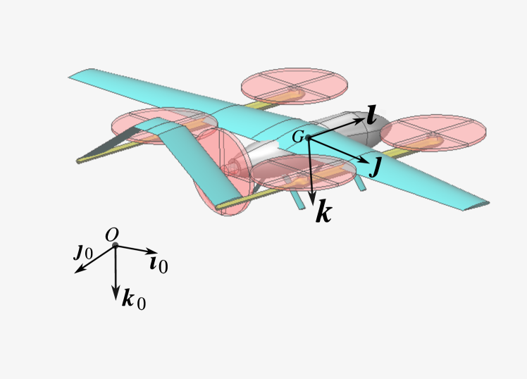
Figure 1: Inertial frame and body-fixed frame axis.

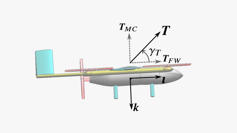
Figure 2: Thrust vectoring representation.

The ordinary differential equations that describe the time evolution of these variables, are obtained by applying the Newton-Euler Formalism, with the earth-fixed frame approximated as being an inertial frame. This yields the following set of kinematic and dynamic equations:

$$\dot{\bm{r}}={\bm{v}}$$ (1)

$$\dot{\bm{v}}={\bm{g}}+\frac{{\bm{F}}_{a}}{m}+\frac{\bm{T}}{m}$$ (2)

$$\frac{d}{dt}(\bm{\imath},\bm{\jmath},\bm{k})={\bm{\omega}}\times(\bm{\imath},\bm{\jmath},\bm{k})$$ (3)

$$J\dot{\omega}=-S(\omega)J\omega+M_{a}+M$$ (4)

Where ${\bm{g}}=g_{0}\bm{k}_{0}$ is the gravity vector, ${\bm{F}}_{a}$ is the resultant aeordynamic force, and ${\bm{T}}$ is the total thrust vector generated by the rotors. $J$ is the body inertia matrix, $M$ is the control torque produced by control surfaces or by propulsion systems, and $M_{a}$ is the residual aerodynamic torque related to the aircraft’s fixed surfaces. Equations (1) to (4) constitute the state equations for our system, with the vectors $\bm{T}$ and $M$ being the control terms.

2.1 Thrust force

Unlike multi-copter or fixed-wing configurations, hybrid VTOLs enable thrust vectoring capabilities via tilt-rotor mechanisms or by being equipped with multiple rotors generating thrust forces in different directions, as is the case for compound configurations. The direction of the total thrust is an additional degree-of-freedom represented here by the angle $\gamma_{T}$ according to Fig. 2. The total thrust force $\bm{T}$ can then be expressed as follows:

$$\bm{T}=|\bm{T}|(\cos(\gamma_{T})\bm{\imath}+\sin(\gamma_{T})\bm{k})$$ (5)

This mathematical representation is valid for both tilt-rotor and compound configurations. In the latter case (see Fig 2) the total thrust force is the sum of the pusher thrust $\bm{T}_{FW}$, and the collective thrust generated by the lift rotors $\bm{T}_{MC}$, i.e. $\bm{T}=\bm{T}_{FW}+\bm{T}_{MC}$. Assuming the pusher rotor is aligned with $\bm{\imath}$, the seperated thrust components can be deduced from $|\bm{T}|$ and $\gamma_{T}$ as follows:

$$\begin{split}\bm{T}_{MC}&=|\bm{T}|\sin(\gamma_{T})\bm{k}\\ \bm{T}_{FW}&=|\bm{T}|\cos(\gamma_{T})\bm{\imath}\end{split}$$ (6)

Also note that these modeling expressions cover the special cases of multi-copter vehicles by fixing $\gamma_{T}$ to $-\pi/2$, and fixed-wing aircraft by fixing $\gamma_{T}$ to zero or to any constant value representing the actual direction of the pusher rotor. For the sake of simplicity, the normal forces that appear in the plane of propellers operating at a non-zero angle of attack are neglected in this control model. However it is possible to approximate these effects as first-order drag forces, as shown in [19].

2.2 Aerodynamic forces

The resultant aerodynamic force $\bm{F}_{a}$ is traditionally decomposed into the sum of a drag and a lift force, or resolved into components along the body frame as following:

$$\bm{F}_{a} =\bm{F}_{X}+\bm{F}_{Y}+\bm{F}_{Z}$$ (7)

$$\bm{F}_{X} =-\frac{1}{2}\rho S|\bm{v}_{a}|^{2}C_{X}~{}\bm{\imath}$$ (8)

$$\bm{F}_{Y} =-\frac{1}{2}\rho S|\bm{v}_{a}|^{2}C_{Y}~{}\bm{\jmath}$$ (9)

$$\bm{F}_{Z} =-\frac{1}{2}\rho S|\bm{v}_{a}|^{2}C_{Z}~{}\bm{k}$$ (10)

Where the aerodynamic coefficients $C_{X}$, $C_{Y}$, and $C_{Z}$ depend on the angle-of-attack $\alpha=atan({\frac{v_{a,3}}{v_{a,1}}})$, and the sideslip angle $\beta=asin({\frac{v_{a,2}}{|\bm{v}_{a}|}})$, as well as on the Reynold and Mach numbers. In this work we consider that the flight conditions are limited to low altitude, and low airspeeds for which compressibility effects can be neglected, this allows to reduce the dependency of the aerodynamic coefficients to $\alpha$ and $\beta$. We also note that we would like to constitute a control model, which allows the design of a cascaded modular control architecture as will be seen in later sections. This motivates the modeling of a triangular system where external control loops do not depend on higher order states. In the case of aerial vehicles, this means that the dependency of $\bm{F}_{a}$ on the angular velocities and control surfaces deflections should be neglected at this stage .

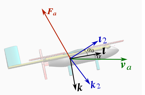
Figure 3: Modified body-axis.

Let $(\bm{\imath}_{2},\bm{\jmath},\bm{k}_{2})$ represent a modified body-fixed frame, with $\bm{\imath}_{2}$ aligned with the zero-lift line of the vehicle i.e. no lift force is generated if the relative air-velocity vector is aligned with $\bm{\imath}_{2}$. We consider that $\bm{\imath}_{2}$ is obtained by rotating $\bm{\imath}$ with an angle $\alpha_{0}$ around $\bm{\jmath}$ as shown in Fig 3 , this gives:

$$\begin{cases}\bm{\imath}_{2}=\cos(\alpha_{0})\bm{\imath}-\sin(\alpha_{0})\bm{k}\\ \bm{k}_{2}=\sin(\alpha_{0})\bm{\imath}+\cos(\alpha_{0})\bm{k}\end{cases},~{}~{}~{}~{}\begin{cases}\bm{\imath}=\cos(\alpha_{0})\bm{\imath}_{2}+\sin(\alpha_{0})\bm{k}_{2}\\ \bm{k}=-\sin(\alpha_{0})\bm{\imath}_{2}+\cos(\alpha_{0})\bm{k}_{2}\end{cases}$$ (11)

Where $\alpha_{0}$ can be defined as the angle between the body-fixed vector $\bm{\imath}$ and the zero-lift line.

Considering the previous definitions and hypothesis, we propose to work with the more specific model of aerodynamic forces previously used in [22],[23],[25], and modified here to account for the zero-lift line:

$$\bm{F}_{a}=-\frac{1}{2}\rho S|\bm{v}_{a}|(c_{0}(\bm{v}_{a}\cdot\bm{\imath}_{2})\bm{\imath}_{2}+\barbar{c}_{0}(\bm{v}_{a}\cdot\bm{\jmath})\bm{\jmath}+\bar{c}_{0}(\bm{v}_{a}\cdot\bm{k}_{2})\bm{k}_{2})$$ (12)

With $c_{0}$, $\bar{c}_{0}$, and $\barbar{c}_{0}$ denoting positive coefficients. As stated in [23] [22], this model is compatible with (12), and corresponds to using $C_{X}=c_{0}\cos(\alpha+\alpha_{0})\cos(\beta)$, $C_{Y}=\barbar{c}_{0}\sin(\beta)$ and $C_{Z}=\bar{c}_{0}\sin(\alpha+\alpha_{0})\cos(\beta)$. These expressions represent bounded non-linear aerodynamic coefficients, that do not grow unbounded when the angles $\alpha$ and $\beta$ get large, hence they remain physically relevant and sufficiently representative for control design purposes by allowing analytical dynamic inversion in the inertial frame as will be seen in later section. Indeed when the sideslip angle is equal to zero, the equivalent lift and drag coefficients are $C_{L}(\alpha)=\frac{1}{2}(\bar{c}_{0}-c_{0})\sin(2(\alpha+\alpha_{0}))$, and $C_{D}(\alpha)=c_{0}+(\bar{c}_{0}-c_{0})\sin^{2}(\alpha+\alpha_{0}).$ When linearizing these expressions with respect to $\alpha$ and $\beta$, one can also deduce the following matches between coefficients: $c_{0}=C_{D,0}$,  $\bar{c}_{0}=C_{D,0}+C_{L,\alpha}$,  and $\barbar{c}_{0}=C_{Y,\beta}$ . The aerodynamic model in 12 isn’t necessarily representative beyond the stall region at high angle of attacks. However when applying this model, the magnitude of the total aerodynamic force that results remains bounded at high airspeed, and it falls towards zero when the airspeed approaches zero where it remains well defined since it does not rely explicitely on $\alpha$ or $\beta$. This is of course a control model on the basis of which analytical flight control expressions will be derived. It remains to design reference trajectories which take into account the flight envelope limitations. For instance in the case of the transition maneuver that goes from zero to cruising speeds, care must be taken to maintain the trimmed angle of attack below the stall region at high airspeed, and only allow higher angles of attack when the airspeed is low enough, and the vehile is in a proper hovering (Multi-Copter) configuration.

2.3 Torque modeling

The aerodynamic torque $M_{a}$ is generally expressed in terms of non-dimensional coefficients (static and stability derivatives) which are themselves functions of $\alpha$, $\beta$ and the components of the angular velocity $\omega$. For the sake of simplicity, we do not expand this torque term and refer interested readers to the literature on the subject e.g. [26] [27]. The control torque $M$ can be considered by itself a control input term. This allows the model and control design to be generalized to a large class of configurations. However we will further develop the expression of $M$ for the compound VTOL configuration as this will constitute our use case in subsequent simulations.

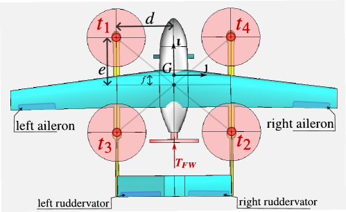
Figure 4: Acturators configuration for a compound VTOL.

Let $M_{MC}$ represent the torque generated by applying differential thrust on the lift rotors, and $M_{FW}$ the torque generated by aerodynamic control surfaces. Therefore, we have $M=M_{MC}+M_{FW}$. It is common to combine the torque vector $M_{MC}$ with the collective thrust generated by the lift rotors $|\bm{T}_{MC}|$ in one vector, that relates to the individual thrust forces $t_{i}$ generated by each rotor. We give the example here for a compound VTOL equipped with four lifting rotors:

$$\begin{bmatrix}|\bm{T}_{MC}|\\ M_{MC}\end{bmatrix}=A\begin{bmatrix}t_{1}\\ t_{2}\\ t_{3}\\ t_{4}\end{bmatrix},~{}~{}~{}~{}~{}A=\begin{bmatrix}1&1&1&1\\ d&-d&d&-d\\ e-f&-e-f&-e-f&e-f\\ \eta&\eta&-\eta&-\eta\end{bmatrix}$$ (13)

Where $d$,$e$ and $f$ are positive scalars characterizing the positions of the rotors with respect to the center of mass as shown in Fig. 4, and $\eta$ is a positive constant approximating the ratio of the power coefficient to the thrust coefficient of the lifting propellers near the hover condition.

Let $M_{FW}$ represent the total aerodynamic torque vector associated with the control surfaces. The vehicle we are considering is equipped with ailerons, and an inversed V-tail consisting of two ruddervators. The former generates principally a roll torque while the latter generate a pitching torque when deflecting in the same direction, and a yawing torque when deflecting in opposite directions. A possible expression for $M_{FW}$ as a function of the ailerons deflection $\delta_{a}$, and the left and right ruddervators deflection $\delta_{rel}$, $\delta_{rer}$ is the following:

$$M_{FW}=\rho|\bm{v}_{a}|^{2}B\begin{bmatrix}\delta_{a}\\ \delta_{rel}\\ \delta_{rer}\end{bmatrix},~{}~{}~{}~{}~{}B=\frac{1}{2}S\begin{bmatrix}bC_{l,\delta_{a}}&bC_{l,\delta_{rel}}&bC_{l,\delta_{rer}}\\ cC_{m,\delta_{a}}&cC_{m,\delta_{rel}}&cC_{m,\delta_{rer}}\\ bC_{n,\delta_{a}}&bC_{n,\delta_{rel}}&bC_{n,\delta_{rer}}\\ \end{bmatrix}$$ (14)

With the control allocation matrix $B$ being a function of control derivatives that are commonly considered to be constants. In nominal conditions, the symmetrical functioning of the ruddervators leads to the following equalities between the coefficients: $C_{m,\delta_{rer}}=C_{m,\delta_{rel}}$ and $C_{n,\delta_{rer}}=-C_{n,\delta_{rel}}$.

3 Control laws design

We start by giving a simplified overview of the control design methodology based on the previously defined control model. Consider first that a feedback control function $\bm{a}_{r}$ is designed in order to achieve an objective related to the trajectory of the vehicle, such that if the translation dynamics equation is $\dot{\bm{v}}(t)=\bm{a}_{r}(\bm{v}(t),\bm{v}_{r}(t))$, the velocity $\bm{v}(t)$ will converge to a desired velocity $\bm{v}_{r}(t)$. The next step consists in solving the required attitude and thrust vector such that the sum of all the forces acting on the vehicule, including aerodynamic forces, results in an acceleration of the vehicle that matches the previously defined control term $\bm{a}_{r}$. In other words, we solve equation ${\bm{a}_{r}}={\bm{g}}+\frac{{\bm{F}}_{a}}{m}+\frac{\bm{T}}{m}$ for the desired attitude of the vehicle represented by ${\mathcal{B}_{r}}=\{G,\bm{\imath}_{r},\bm{\jmath}_{r},\bm{k}_{r}\}$ and the desired thrust vector represented by $(|\bm{T}_{r}|,\gamma_{T,r})$, such that in view of equation 2, the resulting translation dynamics would be $\dot{\bm{v}}(t)=\bm{a}_{r}$ . Finally we design an attitude control function that makes the aircraft frame ${\mathcal{B}}=\{G,\bm{\imath}_{,}\bm{\jmath},\bm{k}\}$ converge to the previously defined desired attitude.

By following this control design methodology we have adopted a hierarchical control architecture with outer position and speed control loops, and inner attitude and angular rate control loops as shown in Fig. 5. A key concept to keep in mind when designing such cascaded loops is the time scale separation, which means that each loop should have relatively faster convergence properties than its outer loop especially when feedforward terms are not transmitted on top of feedback terms. This requirement can be satisfied in the case of aerial vehicles since the inner attitude control loops are fully actuated and can be designed to have higher bandwidth with respect to the under-actuated outer position/speed control loops.

Figure 5: Control Architecture.

Furthermore, hierarchical control offers many advantages by being modular and allowing to use the same control modules for different piloting modes. For instance, the same modules can be applied for a fully autonomous flight, or in the case of a pilot directly commanding speed vector components, altitude setpoints, attitude angles, angular rates, thrust setpoints, or even combinations of the previous commands. It is also worth mentioning the practical benefit linked with facilitating the tuning and failure diagnosis procedures when working with separated lower order systems. In the following subsections, each control module will be detailed by explaining its objective and the associated control law. These control laws build upon previous works in [22] where they were applied to fixed-wing configurations with associated convergence and stability analysis, and then in [24] with an attempt to extend their applicability to convertible VTOLs. Here we adapt these laws to compound VTOL configurations, and modify some control loops, in particular the ’thrust and attitude setpoint computation’ step, which will be designed to be applicable in a unique way across the entire flight envelope, while being compatible with the chosen transition strategy.

3.1 Position Control

In this section we detail the kinematical guidance loops where desired components of the speed vector $\bm{v}$ are computed to allow to achieve an objective related to the positioning of the center of mass of the vehicle. Two main types of position setpoints can be encountered:

• Trajectory: the objective is to track a reference time-varying point in space. This autonomous mode is common for multi-copter vehicles with a hovering flight condition (zero speed) included in their flight domain.

• Path: the objective is to follow a path without time-constraints. The center of mass of the vehicle should approach the path and follow it at a specified speed. This autonomous mode corresponds for example to classical waypoint following operations. It is also preferred for fixed-wing vehicles that apply a specified thrust and/or regulate their airspeed while adjusting their course to follow a desired path.

We choose to separate the problem between a vertical altitude control and a horizontal guidance control. This choice is motivated by the transition strategy that we are aiming for, and by the advantage of being able to maintain a unique altitude control loop functioning continuously all along the transition phase, even when the horizontal guidance switches from a trajectory tracking objective to a path following objective or vice-versa.

3.1.1 Altitude Control

Let $z_{r}(t)$ denote the desired vertical position . The objective of the altitude control module is to define a desired vertical speed $v_{z,r}(t)$ as an intermediate control variable that allows the convergence of the vertical position $z(t)=\bm{p}(t)\cdot\bm{k}_{0}$  to  $z_{r}(t)$, or equivalently the convergence of the tracking error $\tilde{z}=z-z_{r}$ to zero. We propose the following saturated proportional controller:

$$v_{z,r}=sat1D_{v_{z,min}}^{v_{z,max}}(-k_{z}\tilde{z}+\dot{z}_{r})$$ (15)

Where the first feedback term is complemented with the feedforward term $\dot{z}_{r}$, which accounts for time-varying reference inputs. The feedback gain $k_{z}$ is a positive scalar that determines the rate of convergence. The saturation limits $v_{z,min}$ and $v_{z,max}$ are chosen according to the flight envelope specifications of the vehicle and can take different values for multiple flight phases.

3.1.2 Guidance: Trajectory Tracking

Let $\bm{r}_{hor,r}(t)\in(\bm{\imath}_{0},\bm{\jmath}_{0})$ represent the reference position or trajectory of the vehicle in the horizontal plane. The objective of this module is to design an expression for the desired horizontal speed vector $\bm{v}_{hor,r}$ that ensures the convergence of the tracking error $\tilde{\bm{r}}_{hor}=\Pi_{\bm{k}_{0}}\bm{r}-\bm{r}_{hor,r}$ to zero. We propose the following saturated Proportional controller:

$$\bm{v}_{hor,r}=sat^{v_{h,max}}(-k_{p}\tilde{\bm{r}}_{hor}+\dot{\bm{r}}_{hor,r})$$ (16)

Similarly to the altitude controller, we have a feedback term with a positive proportional gain $k_{p}$ complemented with a feedforward term. The desired speed is saturated at $v_{h,max}$.

3.1.3 Guidance: Path Following

Let $(\mathcal{C})$ be a pre-defined geometric path in the horizontal plane. We define the heading of the vehicle by the unitary vector $\bm{h}=\frac{\Pi_{\bm{k}_{0}}\bm{v}}{|\Pi_{\bm{k}_{0}}\bm{v}|}$. The objective of this module is to compute a desired heading of the vehicle denoted by $\bm{h}_{r}\in(\bm{\imath}_{0},\bm{\jmath}_{0})$ that ensures the convergence to zero of the distance between the aircraft’s center of mass and $(\mathcal{C})$. Such approaches called ’vector field strategies’ are well elaborated in the literature. We do not provide a particular solution here since the objective of a path following won’t be necessary for our VTOL transition demonstration, and we refer interested readers to [22], and [28]. We assume here that a desired heading $\bm{h}_{r}$ (mainly constant) will be defined, and bypasses this guidance module if necessary to be treated directly in the following ’Speed Vector Control’ module.

3.2 Speed Vector Control

The inputs for this module take the form of a desired vertical speed $v_{z,r}$ and a horizontal desired velocity expressed as a vector $\bm{v}_{hor,r}$ or as separated horizontal heading reference $\bm{h}_{r}$ and desired horizontal speed $v_{h,r}\in\mathbb{R}^{+}$. These inputs can either come from the outer ’Position Control’ loops, or the outer loops can be bypassed and the inputs set directly here. Two types of horizontal velocity setpoints are identified; this leads to two separated horizontal speed control modules as shown in the following sections, with one of them being activated according to the type of the input. The output of this module is a desired acceleration vector that will serve for the computation of the desired attitude and thrust vector of the vehicle. Therefore, the computation of the desired acceleration is to be viewed as an intermediate step, while the actual intermediate control terms are the attitude and the thrust vector.

3.2.1 Vertical speed Control

The objective of this module is to achieve the convergence of the vertical speed $v_{z}=\bm{v}\cdot\bm{k}_{0}$ to the setpoint $v_{z,r}$ by determining an intermediate desired vertical acceleration $a_{z,r}$. We define the tracking error $\tilde{v}_{z}=v_{z}-v_{z,r}$ and propose the following Proportional/Integral (PI) function:

$$\begin{cases}a_{z,r}=sat1D_{a_{z,min}}^{a_{z,max}}(-k_{vz}\tilde{v}_{z}-I_{vz}+\dot{v}_{z,r})\\ \frac{d}{dt}I_{vz}=\begin{cases}0,~{}\textrm{if}~{}(|I_{vz}|\geq\Delta_{I,vz})\textrm{and}(I_{vz}\tilde{v}_{z}>0)\\ k_{I,vz}\tilde{v}_{z}~{}\textrm{otherwise}\end{cases}\end{cases}$$ (17)

Where $k_{vz}$, and $k_{I,vz}$ are positive proportional and integral gains. $I_{vz}$ is the integral term with its saturation value $\Delta_{I,vz}\in\mathbb{R}^{+}$. This saturation is taken into account to limit anti-windup effects. We also note that we start considering integral terms when dealing with dynamics that are subject to modeling uncertainties. Indeed, integral terms are known to add robustness properties to the control especially with respect to slowly time-varying disturbances. Note also that $a_{z,min}$ and $a_{z,max}$ are chosen to respect the flight envelope of the vehicle.

3.2.2 Horizontal speed Control: Velocity Tracking

The objective of this module is to track a horizontal time-varying velocity vector $\bm{v}_{hor,r}(t)$, by determining an intermediate desired horizontal acceleration $\bm{a}_{hor,r}(t)\in(\bm{\imath}_{0},\bm{\jmath}_{0})$. We define the tracking error by $\tilde{\bm{v}}_{hor}=\Pi_{\bm{k}_{0}}\bm{v}-\bm{v}_{hor,r}$, and propose the following PI function for $\bm{a}_{hor,r}$ :

$$\begin{cases}\bm{a}_{hor,r}=sat^{a_{h,max}}(-k_{vh}\tilde{\bm{v}}_{hor}-\bm{I}_{vh}+\dot{\bm{v}}_{hor,r})\\ \frac{d}{dt}\bm{I}_{vh}=\begin{cases}\bm{0},~{}\textrm{if}~{}(|\bm{I}_{vh}|\geq\Delta_{I,vh})\textrm{and}(\bm{I}_{vh}\cdot\tilde{\bm{v}}_{hor}>0)\\ k_{I,vh}\tilde{\bm{v}}_{hor}~{}\textrm{otherwise}\end{cases}\end{cases}$$ (18)

Where $k_{vh}$ and $k_{I,vh}$ are positive proportional and integral gains, $\bm{I}_{vh}$ is the integral term, and $\Delta_{I,vh}\in\mathbb{R}^{+}$ its associated saturation value. Note that $a_{h,max}$ is the maximum horizontal acceleration value, which indirectly limits the bank angle of the vehicle. For Multi-Copter platforms, and in the absence of aerodynamic forces, it can be shown that the maximum commanded bank angle will correspond to $atan(\frac{a_{h,max}}{g_{0}+a_{z,min}})$ .

3.2.3 Horizontal speed Control: Heading Tracking and Speed Regulation

In this control mode, the horizontal speed control has two objectives:

• Speed regulation: convergence of the aircraft horizontal speed $|\Pi_{\bm{k}_{0}}\bm{v}|$ to a setpoint $v_{h,r}\in\mathbb{R}^{+}$.

• Heading tracking: convergence of the heading $\bm{h}=\frac{\Pi_{\bm{k}_{0}}\bm{v}}{|\Pi_{\bm{k}_{0}}\bm{v}|}$ to the desired heading $\bm{h}_{r}\in(\bm{\imath}_{0},\bm{\jmath}_{0})$.

By definition, we have the following expression for the horizontal acceleration of the aircraft:

$$\begin{cases}\bm{a}_{hor}&=\frac{d}{dt}(\Pi_{\bm{k}_{0}}\bm{v})\\ &=\frac{d}{dt}(|\Pi_{\bm{k}_{0}}\bm{v}|\bm{h})\\ &=\frac{d}{dt}(|\Pi_{\bm{k}_{0}}\bm{v}|)\bm{h}+|\Pi_{\bm{k}_{0}}\bm{v}|(\bm{\omega}_{h}\times\bm{h})\end{cases}$$ (19)

Where, $\bm{\omega}_{h}=\bm{h}\times\dot{\bm{h}}$ denotes the angular velocity of the unitary heading vector $\bm{h}$. On the basis of this expression, we suggest to divide the desired horizontal acceleration $\bm{a}_{hor,r}$ into a tangential acceleration $\bm{a}_{tan,r}$ parallel to $\bm{h}$ and a second lateral acceleration $\bm{a}_{lat,r}$ orthogonal to the previous one. We define the speed regulation error as $e_{v}=|\Pi_{\bm{k}_{0}}\bm{v}|-v_{h,r}$ . An expression for $\bm{a}_{hor,r}$ is then given by the following:

$$\bm{a}_{hor,r}=\bm{a}_{tan,r}+\bm{a}_{lat,r}$$ (20)

with $\bm{a}_{tan,r}$ a saturated PI controller as following:

$$\begin{cases}\bm{a}_{tan,r}&=sat1D^{a_{t,max}}_{a_{t,min}}(-k_{t}e_{v}-I_{v,t}+\dot{v}_{h,r})\bm{h}\\ \frac{d}{dt}I_{v,t}&=\begin{cases}0,~{}\textrm{if}~{}(|I_{v,t}|\geq\Delta_{I,vt})\textrm{and}(I_{v,t}e_{v}>0)\\ k_{I,t}e_{v}~{}\textrm{otherwise}\end{cases}\end{cases}$$ (21)

where $k_{t}$, $k_{I,t}$ are positive gains, $\Delta_{I,vt}$ is the maximum value for the integrator, and $a_{t,min}$, $a_{t,max}$ are limitations for the tangential acceleration. In practice, and especially for fixed-wing platforms it is more common to regulate the airspeed |$\bm{v}_{a}$| instead of the ground speed, by modifying the expression of the regulation error and using $e_{v}=|\bm{v}_{a}|-v_{h,r}$ instead. Indeed, maintaining the airspeed at nominal values helps reducing aerodynamic perturbations, preventing stall conditions, and ensuring an efficient flight condition for which the aircraft has been dimensioned.

A stabilizing feedback expression for $\bm{a}_{lat,r}$ is the following geometric PI controller (see [22]):

$$\begin{cases}\bm{a}_{lat,r}&=sat^{a_{l,max}}(|\Pi_{\bm{k}_{0}}\bm{v}|(\bm{\omega}_{h,r}\times\bm{h}))\\ \bm{\omega}_{h,r}&=k_{h}(\bm{h}\times\bm{h}_{r})+\bm{I}_{h}+(\bm{h}_{r}\times\dot{\bm{h}}_{r})\\ \frac{d}{dt}\bm{I}_{h}&=\begin{cases}\bm{0},~{}\textrm{if}~{}(|\bm{I}_{h}|\geq\Delta_{I,h})\textrm{and}(\bm{I}_{h}\cdot(\bm{h}\times\bm{h}_{r})>0)\\ k_{I,h}(\bm{h}\times\bm{h}_{r})~{}\textrm{otherwise}\end{cases}\end{cases}$$ (22)

where $k_{h}$, $k_{I,h}$ are positive parameters, $\Delta_{I,h}$ is the maximum value for the integrator, and $a_{l,max}$ is the maximum lateral acceleration. It can be shown that the maximum commanded bank angle will correspond approximately to $atan(\frac{a_{l,max}}{g+a_{z,min}})$ .

3.2.4 Thrust Vector and Attitude Setpoints computation

The outputs of the ’Speed Vector Control’ can be summed in a single three-dimensional reference acceleration vector:

$$\bm{a}_{r}=a_{z,r}\bm{k}_{0}+\bm{a}_{hor,r}$$ (23)

This desired acceleration is a stabilizing feedback function for the outer loops. At this point, the objective is to impose this desired acceleration vector, through control terms defined by the thrust vector, and the attitude of the vehicle. Indeed, recalling the translation dynamics equation (2), the objective of imposing $\dot{\bm{v}}=\bm{a}_{r}$ becomes equivalent to solving the following equation:

$$\bm{a}_{r}={\bm{g}}+\frac{{\bm{F}}_{a}}{m}+\frac{\bm{T}}{m}$$ (24)

with $\bm{F}_{a}$ and $\bm{T}$ defined respectively in (12) and (5). Let $\mathcal{B}_{r}=(\bm{\imath}_{r},\bm{\jmath}_{r},\bm{k}_{r})$ represent the desired body frame, and $(|\bm{T}_{r}|,\gamma_{T,r})$ the norm and direction of the desired thrust vector. We propose the solution from [24], that is modified here to become applicable to hovering flights with $\bm{v}_{a}=\bm{0}$. This is done by not relying directly on the angle of attack in the computation of the desired attitude, but on a vector $\bm{a}^{\prime}$ that is always defined along the vehicle’s trajectory. Indeed $\alpha$ becomes ill-defined when the air-velocity $\bm{v}_{a}$ nears zero . In addition, the proposed solution takes into account a misalignement of the zero lift axis with the forward axis of the vehicle $\bm{\imath}$. A detailed proof is reported in appendix 7.1.

We first define the following:

$$\bm{a}^{\prime} =\bm{a}_{r}-\bm{g}$$ (25)

$$\bm{d} =m\bm{a}^{\prime}+\frac{1}{2}\rho S|\bm{v}_{a}|c_{0}\bm{v}_{a}$$ (26)

$$\bm{e} =m\bm{a}^{\prime}+\frac{1}{2}\rho S|\bm{v}_{a}|\bar{c}_{0}\bm{v}_{a}$$ (27)

The expression of $\bm{\jmath}_{r}$ is defined based on one of the two objectives:

• Imposing a desired yaw angle $\psi_{r}$, in which case we propose the following expression for $\bm{\jmath}_{r}$:

  $$\begin{cases}\bm{\jmath}_{r}&=\frac{\bm{h}_{\psi,r}\times\bm{a}^{\prime}}{|\bm{h}_{\psi,r}\times\bm{a}^{\prime}|}\\ \bm{h}_{\psi,r}&=[\cos(\psi_{r}),\sin(\psi_{r}),0]^{\top}\end{cases}$$ (28)

• Zeroing the sideslip angle $\beta$, which corresponds to adopting a ’balanced flight’ or a ’coordinated turn’. This is also equivalent to having the airspeed vector and the aerodynamic forces in the longitudinal plane of the aircraft $(\bm{\imath},\bm{k})$. Therefore $\bm{\jmath}_{r}$ should be orthogonal to both the air-velocity $\bm{v}_{a}$ and the apparent acceleration $\bm{a}^{\prime}$:

  $$\bm{\jmath}_{r}=\frac{\bm{v}_{a}\times\bm{a}^{\prime}}{|\bm{v}_{a}\times\bm{a}^{\prime}|}$$ (29)

  The first objective of tracking a yaw angle is mostly employed when piloting Multi-Copter platforms. In order to avoid the singularity at $|\bm{h}_{\psi,r}\times\bm{a}^{\prime}|=0$, one can choose a value of $a_{z,max}$ (maximum downward acceleration) inferior to the gravity acceleration $g$ in (17). The second objective of a balanced flight is employed in the case of Fixed-Wing platforms that fly at speeds that are sufficient enough to allow the estimation of the air-velocity vector $\bm{v}_{a}$. As discussed in [22], the condition $|\bm{v}_{a}\times\bm{a}^{\prime}|\neq 0$ is not restrictive in practice and includes a much larger set than classicaly defined trim trajectories. In practice, divisions by zero are avoided  .

We exploit here the thrust-vectoring capabilities of VTOL platforms, in two ways, either by imposing the thrust direction $\gamma_{T}$ (as in [24]), or by imposing the equivalent of a pitch angle for the vehicle attitude. We give next the expressions for the control terms that result from the proofs reported in the Appendix.

• case 1: Imposed thrust direction

  Here the value of $\gamma_{T}$ is imposed at $\gamma_{T,r}$. The expressions for the remaining desired body frame axis are the following:

  $$\begin{cases}\bm{k}_{r}&=\sin(\gamma)\frac{\bm{a}^{\prime}}{|\bm{a}^{\prime}|}+\cos(\gamma)\frac{\bm{a}^{{}^{\prime}\perp}}{|\bm{a}^{{}^{\prime}\perp}|}\\ \bm{\imath}_{r}&=\bm{\jmath}_{r}\times\bm{k}_{r}\\ \bm{a}^{{}^{\prime}\perp}&=\bm{a}^{\prime}\times\bm{\jmath}_{r}\\ \gamma&=atan2(y,x)-\alpha_{0}\\ y&=\sin(\gamma_{T,r}+\alpha_{0})\bm{d}\cdot\bm{a}^{\prime}-\cos(\gamma_{T,r}+\alpha_{0})\bm{e}\cdot\bm{a}^{{}^{\prime}\perp}\\ x&=\cos(\gamma_{T,r}+\alpha_{0})\bm{e}\cdot\bm{a}^{\prime}+\sin(\gamma_{T,r}+\alpha_{0})\bm{d}\cdot\bm{a}^{{}^{\prime}\perp}\end{cases}$$ (30)

• case 2: Imposed pitch angle

  Here a desired pitch angle denoted by $\theta_{r}$ is imposed. The expressions for the remaining desired body frame axis, and the desired thrust direction are the following:

  $$\begin{cases}\bm{\imath}_{r}&=\cos(\theta_{r})\bm{\eta}+\sin(\theta_{r})\bm{\eta}^{\perp}\\ \bm{k}_{r}&=\bm{\imath}_{r}\times\bm{\jmath}_{r}\\ \bm{\eta}&=\frac{\bm{\jmath}_{r}\times\bm{k}_{0}}{|\bm{\jmath}_{r}\times\bm{k}_{0}|}\\ \bm{\eta}^{\perp}&=\frac{\bm{\jmath}_{r}\times\bm{\eta}}{|\bm{\jmath}_{r}\times\bm{\eta}|}\\ \gamma_{T,r}&=atan2(y^{\prime},x^{\prime})-\alpha_{0}\\ y^{\prime}&=\sin(\alpha_{0})\bm{e}\cdot\bm{\imath}_{r}+\cos(\alpha_{0})\bm{e}\cdot\bm{k}_{r}\\ x^{\prime}&=\cos(\alpha_{0})\bm{d}\cdot\bm{\imath}_{r}-\sin(\alpha_{0})\bm{d}\cdot\bm{k}_{r}\end{cases}$$ (31)

For both cases the desired thrust norm is given by:

$$\begin{split}|\bm{T}_{r}|=&\cos(\gamma_{T,r}+\alpha_{0})\cos(\alpha_{0})\bm{d}\cdot\bm{\imath}_{r}-\cos(\gamma_{T,r}+\alpha_{0})\sin(\alpha_{0})\bm{d}\cdot\bm{k}_{r}\\ &+\sin(\gamma_{T,r}+\alpha_{0})\sin(\alpha_{0})\bm{e}\cdot\bm{\imath}_{r}+\sin(\gamma_{T,r}+\alpha_{0})\cos(\alpha_{0})\bm{e}\cdot\bm{k}_{r}\end{split}$$ (32)

Convergence analysis for the translation dynamics with the preceding control term expressions is reported in appendix 7.2.

In the case of compound configurations, one can deduce the values for the desired thrusts $|\bm{T}_{MC,r}|$ and $|\bm{T}_{FW,r}|$ from $|\bm{T}_{r}|$ and $\gamma_{T,r}$ using the expressions in (6). Additionally one can impose saturations on the computed thrust values according to the limitations of the rotors capabilities.

Note that the first case of imposing the thrust direction, reduces to conventional Multi-Copter piloting when imposing $\gamma_{T,r}=-\frac{\pi}{2}$ and neglecting the aerodynamic forces (by imposing $c_{0}=0$, and $\bar{c}_{0}=0$). Indeed, we find again the classical geometric control that is widely used today in open-source autopilots, but also in research projects such as [29],[30], [31] and [19]. This same approach is extended to fixed-wing applications by including the aerodynamic forces in the control model, indeed it suffices to fix $\gamma_{T,r}=0$ to find the control proposed in [22]. The general solution presented here is generic, it presents a common control design for different configurations and is therefore particularly suitable for VTOL transition maneuvers with all intermediate states encountered during vehicle reconfiguration.

3.3 Attitude control

The objective of this module is to make the aircraft frame ${\mathcal{B}}=\{G,\bm{\imath},\bm{\jmath},\bm{k}\}$ converge to the desired frame ${\mathcal{B}_{r}}=\{G,\bm{\imath}_{r},\bm{\jmath}_{r},\bm{k}_{r}\}$. This can be done using the following geometric control expression for the desired angular velocity in the inertial frame (see [22]):

$$\begin{cases}\bm{\omega}_{r}&=k_{\mathcal{B}}((\bm{\imath}\times\bm{\imath}_{r})+(\bm{\jmath}\times\bm{\jmath}_{r})+(\bm{k}\times\bm{k}_{r}))+\bm{\omega}_{ff}\\ \bm{\omega}_{ff}&=(\bm{k}_{r}\times\frac{d\bm{k}_{r}}{dt})+((\bm{\jmath}_{r}\times\frac{d\bm{\jmath}_{r}}{dt})\cdot\bm{k}_{r})\bm{k}_{r}\end{cases}$$ (33)

Where $k_{\mathcal{B}}$ is a positive proportional gain and $\bm{\omega}_{ff}$ is a feedforward term that corresponds to the angular velocity associated with the frame ${\mathcal{B}_{r}}$.

An alternative expression for the control term (33), that allows to associate seperate gains with each body-frame axis is the following:

$$\begin{cases}\bm{\omega}_{r}&=k_{\bm{\imath}}(\bm{\omega_{0}}\cdot\bm{\imath})\bm{\imath}+k_{\bm{\jmath}}(\bm{\omega_{0}}\cdot\bm{\jmath})\bm{\jmath}+k_{\bm{k}}(\bm{\omega_{0}}\cdot\bm{k})\bm{k}+\bm{\omega}_{ff}\\ \bm{\omega_{0}}&=(\bm{\imath}\times\bm{\imath}_{r})+(\bm{\jmath}\times\bm{\jmath}_{r})+(\bm{k}\times\bm{k}_{r})\\ \bm{\omega}_{ff}&=(\bm{k}_{r}\times\frac{d\bm{k}_{r}}{dt})+((\bm{\jmath}_{r}\times\frac{d\bm{\jmath}_{r}}{dt})\cdot\bm{k}_{r})\bm{k}_{r}\end{cases}$$ (34)

where $k_{\bm{\imath}}$, $k_{\bm{\jmath}}$ and $k_{\bm{k}}$ can be interpreted as respectively the roll, pitch and yaw proportional gains. A proof for asymptotic convergence associated with this last control term is reported in appendix 7.3.

3.4 Angular rate control

The objective of this module is to make the aircraft’s angular velocity $\bm{\omega}$ converge to the desired angular velocity vector $\bm{\omega}_{r}$. As shown in (4), the attitude dynamics are expressed in the body frame. Thus we elaborate here the control functions using the vectors of coordinates $\omega$ and $\omega_{r}$ expressed in the body frame. We define the tracking error as $\tilde{\omega}=\omega-\omega_{r}$, then on the basis of the state equation (4), we propose the following PI function for a desired control torque $M_{r}$:

$$\begin{cases}M_{r}=-K_{P,\omega}J\tilde{\omega}-I_{\omega}+\omega\times J\omega-M_{a}+J\dot{\omega}_{r}\\ \frac{d}{dt}I_{\omega,i}=\begin{cases}0,~{}\textrm{if}~{}(|I_{\omega,i}|\geq\Delta_{I,\omega_{i}})\textrm{and}(I_{\omega,i}\tilde{\omega}_{i}>0)\\ k_{I,\omega_{i}}~{}\tilde{\omega}_{i}~{}\textrm{otherwise}\\ \textrm{for}~{}i=1,2,3\end{cases}\end{cases}$$ (35)

where $K_{P,\omega}=diag(k_{p,\omega_{1}},k_{p,\omega_{2}},k_{p,\omega_{3}})$, is a diagonal matrix composed of three positive proportional gains. And $k_{I,\omega_{1}}$, $k_{I,\omega_{2}}$ and $k_{I,\omega_{3}}$ are three positive integral gains. The positive scalars $\Delta_{I,\omega_{i}}$ define saturation values for the integrators.

It is possible in practice to omit the cancelation of the aerodynamic torque $M_{a}$. For most aircrafts, this passive torque contributes to the stability of the attitude dynamics around trim trajectories, it is classically taken into account for the tuning of linear controllers, without necessarily being exactly compensated. Furthermore, for some UAV applications, the identification of stability derivatives can be challenging, and an estimation of the vector $M_{a}$ might not be available. However, this should not exclude the possibility to design control laws, especially for the attitude dynamics, which are fully actuated, and can in general tolerate high control gains. For all these reasons, and considering the relatively higher bandwidth of the attitude control loops, we can further neglect the Coriolis and feedforward terms and employ the following alternative expression for $M_{r}$:

$$M_{r}=-K_{P,\omega}J\tilde{\omega}-I_{\omega}$$ (36)

Note that this intermediate step of obtaining a control torque $M_{r}$ is still independent of the actuation configuration of the vehicle.

3.5 Control Allocation Mapping

From this point we give the example of control allocation mapping to the effectors in the case of a compound vehicle as it was modelled in 2.3. The inputs of this module are the commanded thrust vector $\bm{T}_{r}$ divided into two components $\bm{T}_{MC,r}$ and $\bm{T}_{FW,r}$ and the control torque $M_{r}$. Recall that the values for the desired thrusts $|\bm{T}_{MC,r}|$ and $|\bm{T}_{FW,r}|$ can be deduced from from $|\bm{T}_{r}|$ and $\gamma_{T,r}$ using the expressions in (6) as following:

$$|\bm{T}_{MC,r}| =|\bm{T}_{r}||sin(\gamma_{T,r})|$$ (37)

$$|\bm{T}_{FW,r}| =|\bm{T}_{r}||cos(\gamma_{T,r})|$$ (38)

We define the scalar $\lambda\in[0,1]$ as the blending coefficient for torque allocation. When $\lambda$ is set to $0$, the control torque should be generated entirely by the differential thrust of the lifting rotors. On the other hand, when $\lambda$ is set to $1$, the control torque is generated by the aerodynamic control surfaces. This allows to define the distribution of $M_{r}$ between a component $M_{MC,r}$ to be generated by the lifting rotors and a component $M_{FW,r}$ to be generated by the control surfaces. We choose the following continuous blending expressions with respect to $\lambda$:

$$\begin{cases}M_{MC,r}&=(1-\lambda)M_{r}\\ M_{FW,r}&=\lambda M_{r}\end{cases}$$ (39)

The individual thrust values of each lifting rotor, can be computed in accordance with (13), via the inversion of the matrix $A$, i.e.:

$$\begin{bmatrix}t_{1,r}\\ t_{2,r}\\ t_{3,r}\\ t_{4,r}\end{bmatrix}=A^{-1}\begin{bmatrix}|\bm{T}_{MC,r}|\\ M_{MC,r}\end{bmatrix}$$ (40)

The deflection angles of control surfaces, are computed in accordance with (14), as follows:

$$\begin{bmatrix}\delta_{a,r}\\ \delta_{rel,r}\\ \delta_{rer,r}\end{bmatrix}=\frac{1}{\rho|\bm{v}_{a}|^{2}}B^{-1}M_{FW,r}$$ (41)

In practice, desaturation strategies are implemented in addition to the previous allocation mapping in order to deal with situations where certain components of the commanded thrusts or control surfaces angles are outside of their feasible range. We do not detail a specific desaturation strategy in this paper for the sake of brevity and refer the interested reader to the abundant literature on the subject. For instance, the most common algorithms adopt a prioritized policy that favors pitch and roll torque realizations (see [32] and [33]).

4 High Level Transition Strategy

The transition strategy that we propose here, takes the form of successive high-level setpoints, that progressively achieve the reconfiguration of the vehicle from a hovering flight to a high-speed cruise flight and inversely. In this sense, we are exploiting the applicability of the previously designed control loops to the entire flight envelope, and restricting the design activity at this stage to the establishment of an adequate design of transition flight phases.

The sequence of the flight phases are represented in the form of the state machine shown in the Fig. 6. We assume that the vehicle takes off vertically and is piloted as a Multi-Copter vehicle. The pilot or the operator, may then specify the desired heading and initial altitude for the transition, and command the transition profile to be executed according to the state machine with specific parameters that shape the trajectory profile. In a similar way, the pilot or operator can initiate the back-transition maneuver from a cruise flight at a proper location and altitude. Another asset of the proposed transition strategy, is the ability to abort the transition at any intermediate state by progressing towards the appropriate state of the back-transition maneuver. Indeed the transition and back-transition states are designed to be analogous.

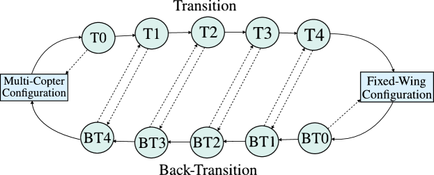
Figure 6: Transition and Back-Transition State Machine.

The forward conditions that clear the passage to the following state, can simply take the form of convergence criteria to desired high-level setpoints. For example, one may specify an acceptable threshold $\epsilon_{\tilde{x}}>0$ for each tracking error $\tilde{x}$, i.e. $|\tilde{x}|<\epsilon_{\tilde{x}}$. The backward conditions represented by dashed lines in Fig. 6, basically abort the transition. This can result from a pilot abort command, a failure detection, a divergence condition, or even ’timeouts’ suggesting an anomaly had occurred during the execution of the phase in question. Tables 2 and 3 describe each of the transition phases (T0 to T4) and the back-transition phases (BT0 and BT4) as well as the associated high-level setpoints.

4.1 Transition flight phases

Table 2: Transition flight phases description

Phase	Description	Setpoints
MC	The vehicle is piloted as a Multi-Copter.	$\gamma_{T,r}=-\frac{\pi}{2}$, $\lambda=0$
T0	Beginning of the transition from a hovering state, a pitch setpoint is specified,	$\theta_{T0}$, $\lambda=0$
	with a desired climb rate, a desired yaw,	$v_{z,T0}<0$, $\psi_{r}$
	and a desired horizontal speed vector increasing in magnitude.	$\bm{v}_{hor,r}$
T1	A pitch setpoint is specified,	$\theta_{T1}$, $\lambda=0$
	with a desired climb rate, sideslip cancellation,	$v_{z,T1}<0$, $\beta=0$
	a desired airspeed, and a desired horizontal heading.	$v_{a,T1}$, $\bm{h}_{r}$
T2	A pitch setpoint is specified, the torque control blended continuously towards	$\theta_{T2}$, $\lambda=0\longrightarrow 1$
	control surfaces, with a desired climb rate, sideslip cancellation,	$v_{z,T2}<0$, $\beta=0$
	a desired airspeed, and a desired horizontal heading.	$v_{a,T1}$, $\bm{h}_{r}$
T3	A pitch setpoint is specified,	$\theta_{T3}$, $\lambda=1$
	with a desired climb rate, sideslip cancellation,	$v_{z,T3}<0$, $\beta=0$
	a desired airspeed increasing towards cruise speed, and a desired horizontal heading.	$v_{a,FW}$, $\bm{h}_{r}$
T4	The vehicle is piloted in a Fixed-Wing configuration,	$\gamma_{T,r}=0$, $\lambda=1$
	at a fixed altitude, with sideslip cancellation,	$z_{r}$, $\beta=0$
	a fixed airspeed at nominal cruise speed, and a desired horizontal heading.	$v_{a,FW}$, $\bm{h}_{r}$
FW	The vehicle is piloted as a Fixed-Wing.	$\gamma_{T,r}=0$, $\lambda=1$

The transition begins with phase T0, where the pitch is imposed to a specific value, which will activate the pusher rotor on top of the lifting rotors in order to push the vehicle forward. A desired horizontal speed vector is specified with an increasing magnitude allowing to reach airspeed values at the end of T0 that are sufficient enough to ensure that $\bm{v}_{a}\neq 0$ and that $\bm{h}$ is well defined. This allows in phase T1 to track a desired heading of the vehicle and to adopt a balanced flight strategy (by zeroing the sideslip). At this point the airspeed is accelerated until it reaches an intermediate value $v_{a,T1}$ for which the aerodynamic control surfaces can produce enough torque actuation for the controllability of the attitude dynamics. The airspeed value $v_{a,T1}$ should also be chosen so that enough collective thrust $T_{MC}$ is produced to avoid reducing differential thrust authority so that a control torque can still be produced simultaneously whether by lifting rotors or control surfaces. Indeed in phase T2, we increase the blending factor $\lambda$ progressively from $0$ to $1$ during a fixed duration (typically two seconds), this will transfer the torque actuation entirely to control surfaces. In phase T3, the vehicle is accelerated towards cruise speed, with a fixed pitch angle $\theta_{T3}$ that is chosen here to be close to the trimming angle-of-attack at nominal cruise speed. During T3 it is expected that the aerodynamic lift force is increasing until it can compensate the weight of the vehicle, so that the thrust generated by the lifting rotors is sharply reduced. Finally, in phase T4 the vehicle is controlled in a pure Fixed-Wing configuration, with a stabilization of its altitude, heading and airspeed.

4.2 Back-Transition flight phases

Table 3: Back-Transition flight phases description

Phase	Description	Setpoints
FW	The vehicle is piloted as a Fixed-Wing.	$\gamma_{T,r}=0$, $\lambda=1$
BT0	The vehicle is piloted in a Fixed-Wing configuration,	$\gamma_{T,r}=0$, $\lambda=1$
	with a desired descent rate, with sideslip cancellation,	$v_{z,BT0}>0$, $\beta=0$
	a fixed airspeed at nominal cruise speed, and a desired horizontal heading.	$v_{a,FW}$, $\bm{h}_{r}$
BT1	A pitch setpoint is specified,	$\theta_{BT1}$, $\lambda=1$
	with a desired descent rate, with sideslip cancellation,	$v_{z,BT1}>0$, $\beta=0$
	a fixed airspeed at nominal cruise speed, and a desired horizontal heading.	$v_{a,FW}$, $\bm{h}_{r}$
BT2	A pitch setpoint is specified,	$\theta_{BT1}$, $\lambda=1$
	with a desired descent rate, with sideslip cancellation,	$v_{z,BT2}>0$, $\beta=0$
	a deceleration towards an intermediate airspeed, and a desired horizontal heading.	$v_{a,BT2}$, $\bm{h}_{r}$
BT3	A pitch setpoint is specified, the torque control blended continuously towards	$\theta_{BT3}$, $\lambda=1\longrightarrow 0$
	differential thrust, at a fixed altitude, with sideslip cancellation,	$z_{BT3}$, $\beta=0$
	at a fixed intermediate airspeed, and a desired horizontal heading.	$v_{a,BT2}$, $\bm{h}_{r}$
BT4	The vehicle is piloted in a Multi-Copter configuration,	$\gamma_{T,r}=-\frac{\pi}{2}$, $\lambda=0$
	at a fixed altitude, with a desired yaw,	$z_{BT4}$, $\psi_{r}$
	and a desired horizontal speed vector decreasing towards zero	$\bm{v}_{hor,r}$
MC	The vehicle is piloted as a Multi-Copter.	$\gamma_{T,r}=-\frac{\pi}{2}$, $\lambda=0$

The back-transition begins with phase BT0 which is essentially a descent phase allowing the aircraft to approach its landing site. In phase BT1, the pitch is imposed, this will activate the lifting rotors, which will allow the vehicle to decelerate its airspeed in BT2 while maintaining the descent rate control without stalling. Indeed the vehicle reaches the intermediate speed $v_{a,BT2}$ which can be chosen equal to $v_{a,T1}$. In BT3 the blending factor is varied progressively from $1$ to $0$ during a fixed duration (typically less than two seconds), this will transmit the generation to torque control entirely to the lifting rotors. The altitude is locked and regulated at its value at the beginning of the phase. Finally in phase BT4 sideslip control is abandoned to yaw control, and the vehicle is piloted as a Multi-Copter with a decelerating horizontal speed towards zero.

Variants of the proposed Transition and Back-Transition state machines can be proposed. For instance, climb and descent rates can be replaced everywhere with a fixed altitude setpoint in order to achieve ’horizontal’ transition maneuvers. One can also choose to keep imposing $\gamma_{T,r}=-\frac{\pi}{2}$ in phase T0, so that the vehicle advances by inclining the collective thrust of the lifting rotors, instead of activating the pusher rotor at this early stage. In order to guarantee a narrow flight corridor, it is also possible to follow a straight horizontal path during the transition and back-transition instead of tracking a fixed heading. Finally, instead of executing the transition and back-transition phases in a complete autonomous mode, it is possible to leave to the pilot or the remote operator the possibility to steer the vehicle in terms of heading, climb or descent rate and airspeed target.

5 Implementation and Hardware-In-The-Loop Simulations

In this section, we test the proposed control laws and transition strategy in a Hardware-In-The-Loop (HIL) simulation. The HIL setup consists of a Matlab/Simulink model of the vehicle connected to a commercially available "Pixhawk 3 Pro" autopilot flight controller, where virtual sensors values are sent to the controller, who in turn computes the actuator’s commands and sends them back, as shown in Fig. 7. The flight control implementation is based on the open-source PX4 flight stack, where the native control modules were replaced by the flight control algorithm and the transition state machine that are presented in this paper. Other functionalities of the PX4 autopilot are kept, in particular the Extended Kalman Filter (EKF) state observer.

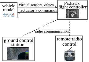
Figure 7: HIL setup.

The targeted vehicle is a commercially available compound VTOL, with a weight of $18Kg$, a wingspan of $3.2m$, and a wing surface of $0.87m^{2}$. It has the same actuators configuration shown in Fig. 4 . A corresponding dynamic model was implemented in the Matlab/Simulink environment, with the aerodynamics forces and torques modelled according to aerodynamic coefficients, and stability and control derivatives themselves estimated using the FlightStream aerodynamic modeling software. The aerodynamic model used in these simulations is more elaborate than the analytical control model (in equation 12) that was used for control design. It is based on look-up tables that cover large angle of attack and sideslip domains, and is complemented with flat plate models outside the domain of convergence of the modeling software via sigmoid blending functions (similarly to [34] chapter 4, or [35]). The thrust forces and shaft torques of the different blades are computed on the basis of a Blade-Element-Momentum-Theory (BEMT) model, see [36] or [27] for example . Typical time constants and power limitations are also included in the dynamic modeling of the control surfaces and of the electrical motors.

5.1 Practical Considerations

5.1.1 Estimation of the air-velocity vector

The peculiarity of UAVs is that they are usually not equipped with angle of attack and sideslip sensors. There is typically a pitot tube that measures a pressure difference translated into the airspeed component $v_{a,1}$. The control laws rely on the air-velocity vector $\bm{v}_{a}$, which requires estimating this vector despite the absence of angle of attack and sideslip sensors. There are several methods to solve this problem, they are mainly classified into two categories, model-based estimators (see [37] for example, or the method proposed in [22]) and kinematic estimators (see [38] for example). We propose here a simple kinematic method that exploits the measurement of the inertial speed $\bm{v}$, and assumes that the wind is horizontal and has no vertical component. It is also considered that sideslip remains low thanks to the passive stability of the airplane’s geometry (weather vane effects via its vertical stabilizer and wing dihedral). The estimation error due to this assumption should be compensated by the robustness of the control terms thanks to the use of integral terms.
We denote the estimated air-velocity and inertial speed vectors by $\hat{\bm{v}}_{a}$, and $\hat{\bm{v}}$ respectively. The assumption of a horizontal wind, implies that the vertical component of the air-velocity equals that of the inertial speed as follows:

$$\bm{\hat{}}{v}_{a}\cdot\bm{k}_{0}=\hat{\bm{v}}\cdot\bm{k}_{0}$$ (42)

Now replacing $\bm{v}_{a}$ with its decomposition in the body fixed-frame gives:

$$\hat{v}_{a,1}~{}\bm{\imath}\cdot\bm{k}_{0}+\hat{v}_{a,2}~{}\bm{\jmath}\cdot\bm{\jmath}_{0}+\hat{v}_{a,3}~{}\bm{k}\cdot\bm{k}_{0}=\hat{\bm{v}}\cdot\bm{k}_{0}$$ (43)

While the component $\hat{v}_{a,1}$ is considered to be obtained from the pitot tube measurement, we set $\hat{v}_{a,2}=0$ in accordance with the previous assumptions. The resulting expression for $\hat{v}_{a,3}$ is deduced from (43) as follows:

$$\hat{v}_{a,3}=\frac{\hat{\bm{v}}\cdot\bm{k}_{0}-\hat{v}_{a,1}~{}\bm{\imath}\cdot\bm{k}_{0}}{\bm{k}\cdot\bm{k}_{0}}$$ (44)

The resulting approximation of $\bm{v}_{a}$ is then $\hat{\bm{v}}_{a}=\hat{v}_{a,1}~{}\bm{\imath}+\hat{v}_{a,3}~{}\bm{k}$. It is of course necessary to avoid dividing by zero when $\bm{k}\cdot\bm{k}_{0}=0$, this can be done in practice by multiplying by $\frac{\bm{k}\cdot\bm{k}_{0}}{(\bm{k}\cdot\bm{k}_{0})^{2}+\epsilon}$ where $\epsilon$ is a small number, instead of the division. Moreover this singularity occurs at bank angles near $90^{\circ}$. This flight condition is clearly outside the flight envelope of the vehicle especially during the transition maneuver and should be avoided by choosing proper limitations on desired acceleration terms in the ’speed vector control’ module.

5.1.2 Translation to Pulse-Width-Modulation (PWM) signals

The outputs of the flight controller for commercial UAVs are generally PWM electronic square signals, that are encoded in the autopilot software as values comprised between $1000\mu s$ and $2000\mu s$ representing the period of time of the ’on’ state. The control terms that are computed need to be translated into corresponding PWM values. This means that for rotors, the desired thrust value $t_{i}$ (or $T_{FW}$ for the pusher rotor) should be transformed to the right PWM encoded value. The same applies for the deflection of control surfaces who are first computed as angles. In this research work, we first estimated the functions giving a control term $u$ as function of the applied PWM signal, i.e $u=f_{u}(PWM_{u})$, this was done by combining datasheet information with ground tests of the actuators. The next step consisted in inversing the previous relation, i.e. estimating the functions in the form $PWM_{u}=f_{u}^{-1}(u)$ that allows to deduce a command value $PWM_{u}$ for every desired actuation command $u$. Note that $f_{u}^{-1}$ can be obtained through a polynomial correlation, or even a tabulated interpolation.

5.2 Control parameters and simulation results

The control parameters used in the control laws are shown in table 4 . One can notice that a single set of parameters is applied for the entire flight envelope without the need for gain scheduling. This is made possible by the nonlinear aspect of the control design which is model-based and takes into account instaneous values of speed, airspeed and dynamic pressure (in equations (22), (26), (27) and (41) for instance). However, this is not guaranteed to be the case for all applications, especially for larger vehicles with lower actuator bandwidth. Typically, stability and robustness analysis can be peformed to validate parameters tuning and scheduling. Such assessment methods may involve frequency-domain analysis such as evaluation of stability margins and disturbation rejection bandwidth, or time-domain analysis using Monte-Carlo simulations to assess robustness in the presence of parameter dispersions. We refer the interested reader to the abundant literature on the subject (see for example [39] and [40]), and we focus in this paper on presenting the contributions of the proposed control approach.

The parameter $\lambda\in[0,1]$, which represents the blending coefficient for torque actuation, was varied smoothly and linearly. During phase T2, it was increased from $0$ to $1$ in two seconds according to the expression $\lambda(\Delta t)=min(0.5\Delta t,1)$, with $\Delta t$ the elapsed time since the beginning of T2. During phase BT3, it was decreased from $1$ to $0$ in one second according to the expression $\lambda(\Delta t)=max(1-\Delta t,0)$, with $\Delta t$ the elapsed time since the beginning of BT3.

Table 4: Control parameters

Control Module	Gains
Altitude Control	$k_{z}=0.25$, $v_{z,max}=1$, $v_{z,min}=-1.5$
Guidance, trajectory tracking	$k_{p}=0.29$, $v_{h,max}=5$
Vertical speed control	$k_{v,z}=3.65$, $k_{I,vz}=1.25$, $a_{z,max}=4.5$, $a_{z,min}=-5.5$, $\Delta_{I,vz}=3.15$
Horizontal speed control	$k_{v,h}=1.5$, $k_{I,vh}=0.7$, $a_{h,max}=3.35$, $\Delta_{I,vh}=2.75$
Velocity tracking
Horizontal speed control	$k_{t}=2.4$, $k_{I,t}=1.1$, $a_{t,max}=5$, $a_{t,min}=-1$, $\Delta_{I,vt}=1.3$, $k_{h}=0.8$, $k_{I,h}=0.16$,
Path following	$a_{l,max}=5.21$, $\Delta_{I,h}=1.5$
Model parameters	$m=17.5$, $\rho=1.2$, $c_{0}=0.074$, $\bar{c}_{0}=5.074$, $S=0.868$, $\alpha_{0}=4.53^{\circ}=0.0791~{}rad$
Attitude control	$k_{\bm{\imath}}=6$, $k_{\bm{\jmath}}=6$, $k_{\bm{k}}=1.8$
Angular rates control	$k_{p,\omega_{1}}=11$, $k_{p,\omega_{2}}=12$, $k_{p,\omega_{3}}=4.75$, $k_{I,\omega_{1}}=10$, $k_{I,\omega_{2}}=25$, $k_{I,\omega_{3}}=0.15$,
	$\Delta_{I,\omega_{1}}=3.5$, $\Delta_{I,\omega_{2}}=8$, $\Delta_{I,\omega_{3}}=0.5$
Actuators and inertia	$d=0.55$, $e=0.55$, $f=0.025$, $b=3.2$, $c=0.3$, $\eta=0.021$, $C_{l,\delta_{a}}=0.002$,
	$C_{l,\delta_{rel}}=C_{l,\delta_{rer}}=0$, $C_{m,\delta_{a}}=0$, $C_{m,\delta_{rel}}=C_{m,\delta_{rer}}=0.006$,
	$C_{n,\delta_{rer}}=-C_{n,\delta_{rel}}=0.0018$, $J=diag(0.87,1.11,1.84)$

The chosen flight scenario consists of five consecutive parts:

1. Multi-Copter (MC) mode: this phase consists of a manual Takeoff until hovering at a fixed altitude, with the pilot sending position and inertial speed commands, and the control modules running in a ’Multi-Copter’ mode, neglecting aerodynamic compensation, and imposing a thrust direction i.e. $\gamma_{T,r}=-\frac{\pi}{2}$, and a torque control achieved throught differential thrust i.e. $\lambda=0$ .

2. Transition: here the pilot triggers the transition (phases T0 to T4) which is achieved autonomously along the initial heading.

3. Fixed-Wing (FW) mode: in this phase the pilot is commanding the vehicle by sending airspeed, heading and altitude (or climb and descent rate) setpoints. The control modules are running in a ’Fixed-Wing’ mode, taking into account aerodynamic compensation, and imposing a thrust direction i.e. $\gamma_{T,r}=0$, and a torque control achieved through control surfaces i.e. $\lambda=1$ .

4. Back-Transition: here the pilot triggers the back-transition (phases BT0 to BT4) which is achieved autonomously along the intial heading.

5. Multi-Copter (MC) mode: in this phase the pilot is again taking control similarly to the first phase, with the intention to manually land the vehicle, with the control modules imposing $\gamma_{T,r}=-\frac{\pi}{2}$ and $\lambda=0$ .

A steady wind is added to the simulation, in such a manner that during the transition maneuver, a front wind is blowing at $3m/s$ which becomes a rear wind during the back transition. Both the transition and back transition experience a lateral wind blowing at $1m/s$. In order to further test the robustness of the control, the simulated weight of the vehicle has been increased to $19Kg$ while the value ’viewed’ by the control modules remained at $m=17.5Kg$.

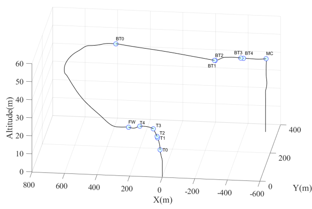
Figure 8: Aircraft’s trajectory.

Simulation results reported in the Figures 8 to 15, show that the control modules successfully achieved the transition and back-transition maneuvers progressively. The different setpoints were tracked with acceptable errors magnitudes in all the phases, as well as in manually piloted MC and FW phases. We notice that the desired deceleration of the airspeed during phase BT2 can’t be achieved at the required rate, that is due to the physical impossibility to achieve negative thrust with the pusher rotor, however this does not preclude the pursuit of the back-transition and the deceleration of the vehicle towards a hover flight condition.

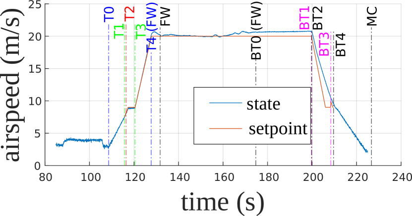
Figure 9: Airspeed.

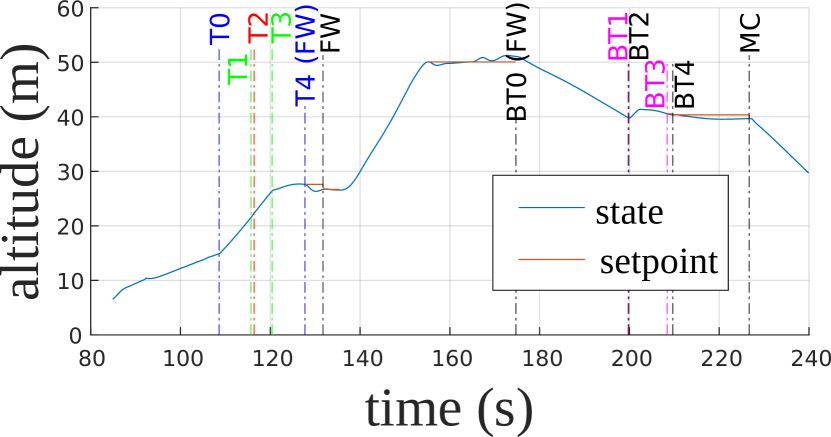
Figure 10: Altitude.

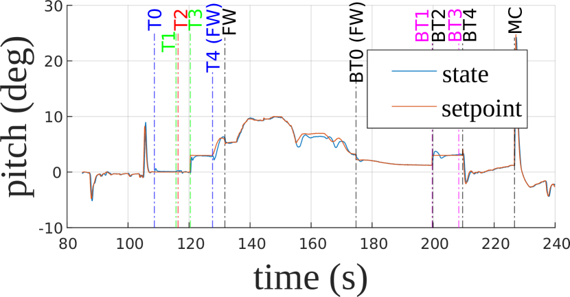
Figure 11: Pitch angle.

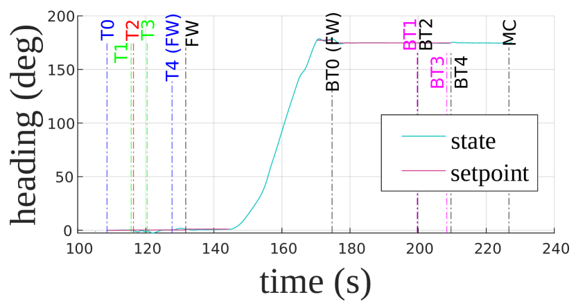
Figure 12: Heading of the vehicle with respect to axis $\bm{\imath}_{0}$

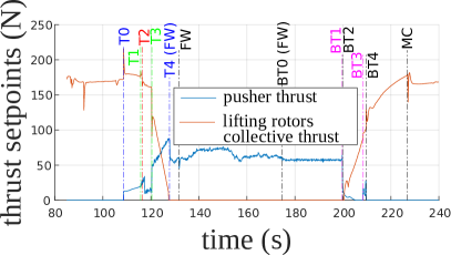
Figure 13: Collective Multi-Copter thrust ($|\bm{T}_{MC,r,}|$) and pusher thrust ($|\bm{T}_{FW,r,}|$) commands.

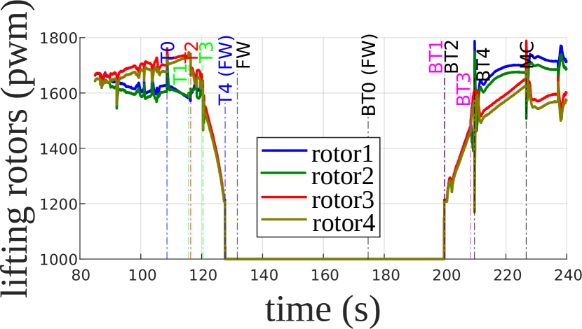
Figure 14: Lifting rotors PWM commands.

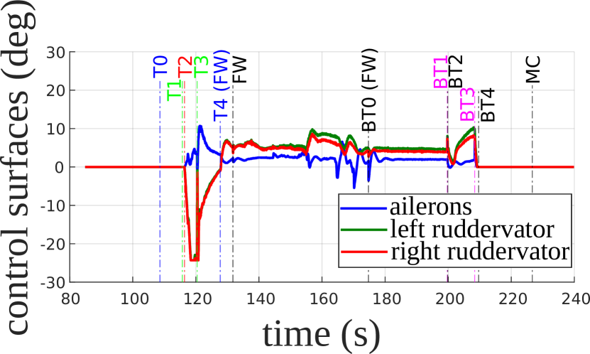
Figure 15: Control surfaces commands.

6 Flight Experiment

In this section, we experimentally test the transition maneuvers, with the flight controller integrated on board the compound VTOL shown in figure 16. During the experiment, a wind with an average magnitude of $3m/s$ was blowing from the east. After performing a manual takeoff in a Multi-Copter configuration, the pilot aligned the vehicle to face the coming wind and triggered the transition phase. Then, after having reached the final step (T4) of the transition in which the vehicle was flying autonomously in a Fixed-Wing configuration, the pilot initiated the back-transition maneuver. The vehicle was eventually decelerated to a hovering flight, after which it was manually landed.

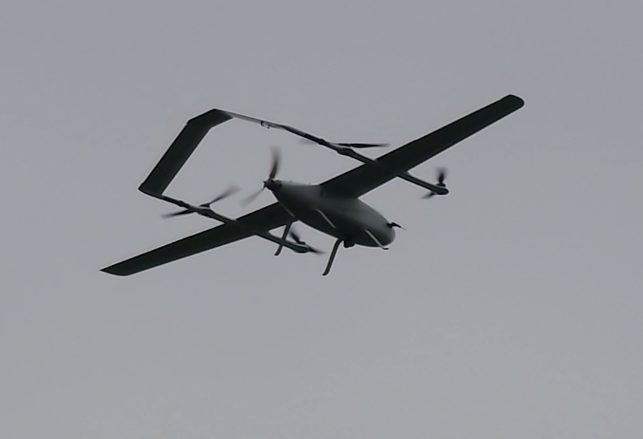
Figure 16: The VTOL UAV during the experiment.

Figures 17 to 24 show that the transition strategy and control laws succeeded in achieving the reconfiguration of the vehicle between the Multi-Copter and Fixed-Wing configurations. The desired heading is tracked with an error of less than $3^{\circ}$, which has resulted in an almost longitudinal flight respecting a narrow flight corridor. Also, note that no loss of altitude is experienced during the transition, and the airspeed is accelerated in accordance with the varying airspeed setpoint. A tracking error on the desired pitch can be noticed during the beginning of the transition and the end of the back-transition. This was attributed to downwash effects on the rear lifting rotors when flying at high airspeeds, which decreases their efficiency and leads to a positive torque offset. This highlights the complexity of designing such VTOL configurations that has to take into account complex aerodynamic interactions. However, the pitch tracking error did not prevent the vehicle from achieving the transition by accelerating to higher airspeeds at which aerodynamic control surfaces become sufficiently efficient to restore control robustness.

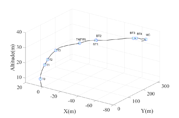
Figure 17: Aircraft’s trajectory.

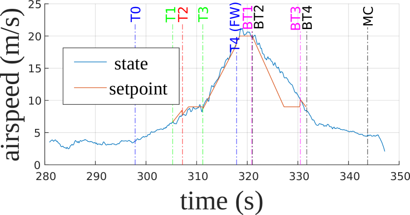
Figure 18: Airspeed.

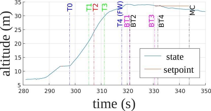
Figure 19: Altitude.

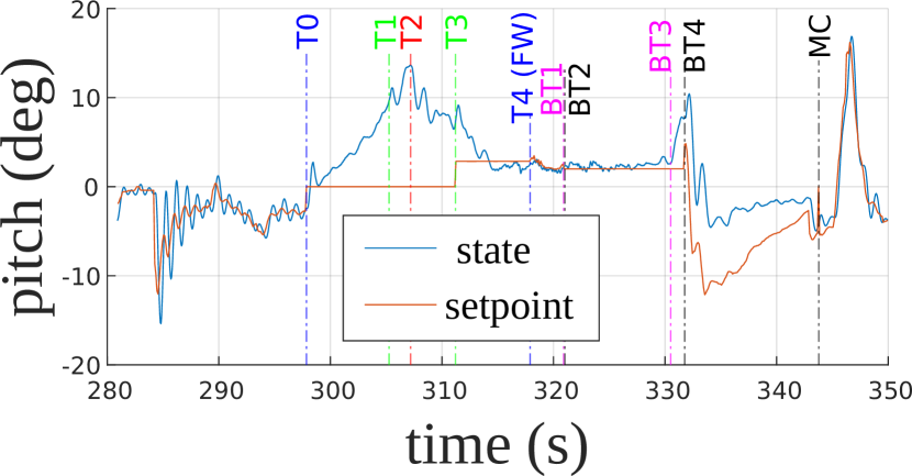
Figure 20: Pitch angle.

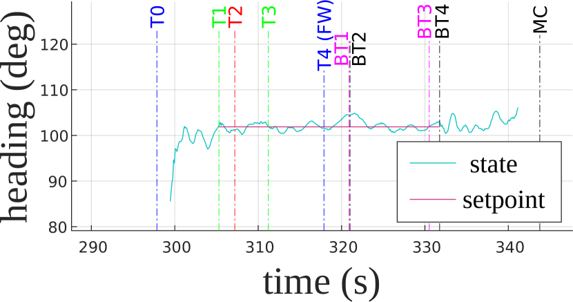
Figure 21: Heading of the vehicle with respect to axis $\bm{\imath}_{0}$

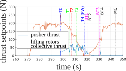
Figure 22: Collective Multi-Copter thrust ($|\bm{T}_{MC,r,}|$) and pusher thrust ($|\bm{T}_{FW,r,}|$) commands.

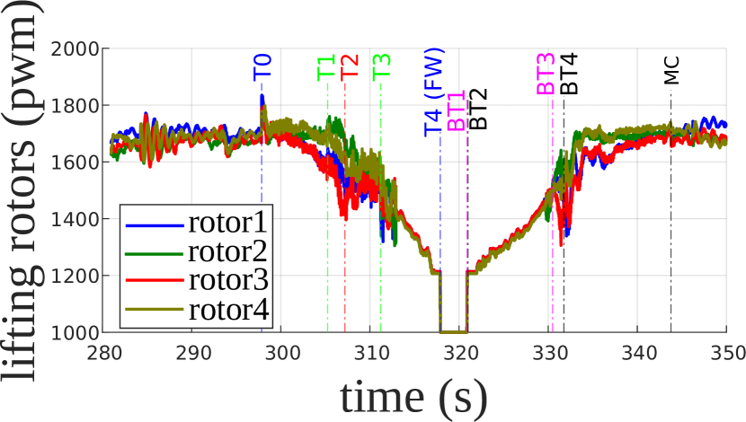
Figure 23: Lifting rotors PWM commands.

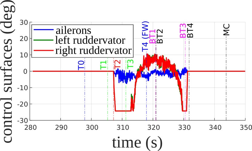
Figure 24: Control surfaces commands.

7 Conclusion

A flight control design and a transition strategy for compound eVTOLs was presented. The control laws are generic and applicable to any vehicle configuration whether it is a Multi-Copter, a Fixed-Wing or a VTOL with additional actuation capabilities and multiple means for torque generation. This control design was detailed for the compound VTOL configuration and was associated with a sequence of high-level setpoints in order to constitute a transition strategy that exploits the convergence and stability properties of the control laws throughout the intermediate transition states. Simulation results and flight experiments show the strategy’s potential to provide stable transition maneuvers, which makes it eligible to satisfy narrow flight corridor requirements and adds the capability to abandon the transition and back transition phases at any intermediate point of the maneuvers.

Appendix

7.1 Proof for the thrust vector and attitude setpoints computation

Here we give proofs for the expressions corresponding to equations (30), (31) and (32).The following proof differs from the work in [24] by computing the orientation of the desired body axis with respect to the apparent acceleration $\bm{a}^{\prime}$ instead of the air-velocity vector $\bm{v}_{a}$. This allows to define the control terms even when $\bm{v}_{a}$ is equal to zero. Another difference with [24], is the possibility to impose a pitch angle, as reported in the second case. Recall that the objective is to solve the following equation:

$$\bm{a}^{\prime}=\frac{{\bm{F}}_{a}}{m}+\frac{\bm{T}_{r}}{m}$$ (45)

We report here the previous definitions of the aerodynamic force model $\bm{F}_{a}$, and the vectors $\bm{a}^{\prime}$, $\bm{d}$ and $\bm{e}$:

$$\bm{F}_{a} =-\frac{1}{2}\rho S|\bm{v}_{a}|(c_{0}(\bm{v}_{a}\cdot\bm{\imath}_{2r})\bm{\imath}_{2r}+\barbar{c}_{0}(\bm{v}_{a}\cdot\bm{\jmath}_{r})\bm{\jmath}_{r}+\bar{c}_{0}(\bm{v}_{a}\cdot\bm{k}_{2r})\bm{k}_{2r})$$ (46)

$$\bm{a}^{\prime} =\bm{a}_{r}-\bm{g}$$ (47)

$$\bm{d} =m\bm{a}^{\prime}+\frac{1}{2}\rho S|\bm{v}_{a}|c_{0}\bm{v}_{a}$$ (48)

$$\bm{e} =m\bm{a}^{\prime}+\frac{1}{2}\rho S|\bm{v}_{a}|\bar{c}_{0}\bm{v}_{a}$$ (49)

Replacing these expressions in equation (45) yields:

$$(\bm{d}\cdot\bm{\imath}_{2r}-|\bm{T}_{r}|\cos(\gamma_{T,r}+\alpha_{0}))\bm{\imath}_{2r}+(\bm{e}\cdot\bm{k}_{2r}-|\bm{T}_{r}|\sin(\gamma_{T,r}+\alpha_{0}))\bm{k}_{2r}+(\bm{a}^{\prime}\cdot\bm{\jmath}_{r}+\frac{1}{2}\rho S|\bm{v}_{a}|\barbar{c}_{0}v_{a,2})\bm{\jmath}_{r}=0$$ (50)

With the chosen expressions of $\bm{\jmath}_{r}$ in section 3.2.4, and especially the expression employed in the presence of aerodynamic forces, i.e. equation (29), the last term in (50) equals zero. The equality in (50) becomes equivalent to solving the following system:

$$\begin{cases}\bm{d}\cdot\bm{\imath}_{2r}-|\bm{T}_{r}|\cos(\gamma_{T,r}+\alpha_{0})&=0\\ \bm{e}\cdot\bm{k}_{2r}-|\bm{T}_{r}|\sin(\gamma_{T,r}+\alpha_{0})&=0\end{cases}$$ (51)

Which is also equivalent to:

$$\begin{cases}(\bm{d}\cdot\bm{\imath}_{2r})\sin(\gamma_{T,r}+\alpha_{0})-(\bm{e}\cdot\bm{k}_{2r})\cos(\gamma_{T,r}+\alpha_{0})=0\\ |\bm{T}_{r}|=\cos(\gamma_{T,r}+\alpha_{0})(\bm{d}\cdot\bm{\imath}_{2r})+\sin(\gamma_{T,r}+\alpha_{0})(\bm{e}\cdot\bm{k}_{2r})\end{cases}$$ (52)

With the additional degree of freedom provided by the thrust direction term $\gamma_{T}$, there exists an infinity of solutions for the system (52). We restrict the analysis for the two cases considered in this paper.

• case 1: Imposed thrust direction $\gamma_{r}$ We recall the definition of $\bm{a}^{{}^{\prime}\perp}$:

  $$\bm{a}^{{}^{\prime}\perp}=\bm{a}^{\prime}\times\bm{\jmath}_{r}$$ (53)

  We consider that $\bm{\imath}_{r}$ can be obtained by rotating $\frac{\bm{a}^{\prime}}{|\bm{a}^{\prime}|}$ around $\bm{\jmath}_{r}$ with an angle $\gamma$ as shown in Fig. 25.

  

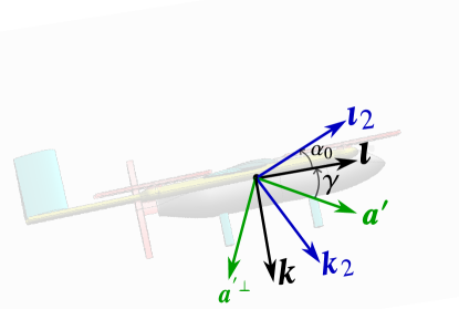
  Figure 25: Definitions of angles $\gamma$ and $\alpha_{0}$. Note that the shown angles are positive according to the chosen convention.

  This gives:

  $$\begin{cases}\bm{\imath}_{r}&=\cos{\gamma}\frac{\bm{a}^{\prime}}{|\bm{a}^{\prime}|}-\sin{\gamma}\frac{\bm{a}^{{}^{\prime}\perp}}{|\bm{a}^{{}^{\prime}\perp}|}\\ \bm{k}_{r}&=\sin{\gamma}\frac{\bm{a}^{\prime}}{|\bm{a}^{\prime}|}+\cos{\gamma}\frac{\bm{a}^{{}^{\prime}\perp}}{|\bm{a}^{{}^{\prime}\perp}|}\end{cases}$$ (54)

  The solution to the problem can then be given by:

  $$\begin{cases}\bm{k}_{r}&=\sin{\gamma}\frac{\bm{a}^{\prime}}{|\bm{a}^{\prime}|}+\cos{\gamma}\frac{\bm{a}^{{}^{\prime}\perp}}{|\bm{a}^{{}^{\prime}\perp}|}\\ \bm{\imath}_{r}&=\bm{\jmath}_{r}\times\bm{k}_{r}\end{cases}$$ (55)

  From here it suffices to solve the first equation in (52) for $\gamma$. Given the previous definition of angle $\alpha_{0}$ in section 2.2, we can write the following:

  $$\begin{cases}\bm{\imath}_{2r}&=\cos({\gamma+\alpha_{0}})\frac{\bm{a}^{\prime}}{|\bm{a}^{\prime}|}-\sin({\gamma+\alpha_{0}})\frac{\bm{a}^{{}^{\prime}\perp}}{|\bm{a}^{{}^{\prime}\perp}|}\\ \bm{k}_{2r}&=\sin({\gamma+\alpha_{0}})\frac{\bm{a}^{\prime}}{|\bm{a}^{\prime}|}+\cos({\gamma+\alpha_{0}})\frac{\bm{a}^{{}^{\prime}\perp}}{|\bm{a}^{{}^{\prime}\perp}|}\end{cases}$$ (56)

  Replacing equations (56) in the first equation of the system (52), we get:

  $$\begin{cases}\cos(\gamma+\alpha_{0})(\sin(\gamma_{T,r}+\alpha_{0})(\bm{d}\cdot\bm{a}^{\prime})-\cos(\gamma_{T,r}+\alpha_{0})\bm{e}\cdot\bm{a}^{{}^{\prime}\perp})\\ -\sin(\gamma+\alpha_{0})(\sin(\gamma_{T,r}+\alpha_{0})\bm{d}\cdot\bm{a}^{{}^{\prime}\perp}+\cos(\gamma_{T,r}+\alpha_{0})\bm{e}\cdot\bm{a}^{\prime})=0\end{cases}$$ (57)

  Or equivalently:

  $$\begin{cases}\gamma&=atan2(y,x)-\alpha_{0}\\ y&=\sin(\gamma_{T,r}+\alpha_{0})\bm{d}\cdot\bm{a}^{\prime}-\cos(\gamma_{T,r}+\alpha_{0})\bm{e}\cdot\bm{a}^{{}^{\prime}\perp}\\ x&=\cos(\gamma_{T,r}+\alpha_{0})\bm{e}\cdot\bm{a}^{\prime}+\sin(\gamma_{T,r}+\alpha_{0})\bm{d}\cdot\bm{a}^{{}^{\prime}\perp}\end{cases}$$ (58)

• case 2: Imposed pitch angle $\theta_{r}$:

  First, we recall the definition of the horizontal unitary vector $\bm{\eta}$ that is orthogonal to $\bm{\jmath}_{r}$:

  $$\bm{\eta}=\frac{\bm{\jmath}_{r}\times\bm{k}_{0}}{|\bm{\jmath}_{r}\times\bm{k}_{0}|}$$ (59)

  The unitary vector $\bm{\eta}^{\perp}$ that is orthogonal to both $\bm{\eta}$ and $\bm{\jmath}_{r}$ is given by:

  $$\bm{\eta}^{\perp}=\frac{\bm{\jmath}_{r}\times\bm{\eta}}{|\bm{\jmath}_{r}\times\bm{\eta}|}$$ (60)

  Since $\bm{\eta}$ is horizontal, an expression for the body axis $\bm{\imath}_{r}$ that corresponds to a pitch angle of $\theta_{r}$, can be expressed in the frame $(\bm{\eta},\bm{\eta}^{\perp})$ as:

  $$\bm{\imath}_{r}=\cos(\theta_{r})\bm{\eta}+\sin(\theta_{r})\bm{\eta}^{\perp}$$ (61)

  Then, $\bm{k}_{r}$ can be deduced as $\bm{k}_{r}=\bm{\imath}_{r}\times\bm{\jmath}_{r}$. It remains to find the solution for the thrust angle $\gamma_{T,r}$. The first equation in (52), is equivalent to:

  $$\gamma_{T,r}+\alpha_{0}=atan2(\bm{e}\cdot\bm{k}_{2r},\bm{d}\cdot\bm{\imath}_{2r})$$ (62)

  Using the expressions of the modified body axis in (11), and replacing them in (62), we find the expression for the desired thrust direction $\gamma_{T,r}$ as expressed in (31).

For the two preceding cases (imposed thrust direction and imposed pitch angle), the solution for the thrust norm $|\bm{T}_{r}|$ as function of the desired body axis $(\bm{\imath}_{r},\bm{k}_{r})$ can be obtained by combining (11) with the second equation in (52) to give the expression in (32).

7.2 Convergence analysis for the translation dynamics

Here we analyse the convergence of the translation dynamics. The objective is to reduce the closed-loop equation of the translation dynamics to the form:

$$\dot{\bm{v}}=\bm{a}_{r}+\bm{o}(t),~{}~{}\displaystyle{\lim_{t\to\infty}}\bm{o}(t)=0$$ (63)

with $\bm{a}_{r}$ a feedback control law equivalent to a desired acceleration vector that asymptotically (and locally exponentially) stabilizes the position and velocity tracking errors at zero, and $\bm{o}(t)$ a sum of additive perturbation terms that asymptotically (and locally exponentially) converges to $0$.

From equation 2 we have:

$$\dot{\bm{v}}={\bm{g}}+\frac{{\bm{F}}_{a}}{m}+\frac{\bm{T}}{m}$$ (64)

By combining the definition of $\bm{a}^{\prime}$ from equation 47 with equation 64, one can write:

$$\dot{\bm{v}}=\bm{a}_{r}-\bm{a}^{\prime}+\frac{{\bm{F}}_{a}}{m}+\frac{\bm{T}}{m}$$ (65)

We report again the definitions of the aerodynamic force model $\bm{F}_{a}$, the thrust vector $\bm{T}$ and the vectors $\bm{d}$ and $\bm{e}$:

$$\bm{F}_{a} =-\frac{1}{2}\rho S|\bm{v}_{a}|(c_{0}(\bm{v}_{a}\cdot\bm{\imath}_{2})\bm{\imath}_{2}+\barbar{c}_{0}(\bm{v}_{a}\cdot\bm{\jmath})\bm{\jmath}+\bar{c}_{0}(\bm{v}_{a}\cdot\bm{k}_{2})\bm{k}_{2})$$ (66)

$$\bm{T} =|\bm{T}|(\cos(\gamma_{T}+\alpha_{0})\bm{\imath}_{2}+\sin(\gamma_{T}+\alpha_{0})\bm{k}_{2})$$ (67)

$$\bm{d} =m\bm{a}^{\prime}+\frac{1}{2}\rho S|\bm{v}_{a}|c_{0}\bm{v}_{a}$$ (68)

$$\bm{e} =m\bm{a}^{\prime}+\frac{1}{2}\rho S|\bm{v}_{a}|\bar{c}_{0}\bm{v}_{a}$$ (69)

Replacing these expressions in equation (65) yields:

$$\dot{\bm{v}}=\bm{a}_{r}-\frac{1}{m}(\bm{d}\cdot\bm{\imath}_{2}-|\bm{T}|\cos(\gamma_{T}+\alpha_{0}))\bm{\imath}_{2}-\frac{1}{m}(\bm{e}\cdot\bm{k}_{2}-|\bm{T}|\sin(\gamma_{T}+\alpha_{0}))\bm{k}_{2}-\frac{1}{m}(\bm{a}^{\prime}\cdot\bm{\jmath}+\frac{1}{2}\rho S|\bm{v}_{a}|\barbar{c}_{0}\bm{v}_{a}\cdot\bm{\jmath})\bm{\jmath}$$ (70)

Recalling the relations from 51 for the solutions of $|\bm{T}_{r}|$, $\gamma_{T,r}$, $\bm{\imath}_{2r}$ and $\bm{k}_{2r}$, and using the fact that $\bm{\jmath}_{r}$ is orthogonal to both $\bm{a}^{\prime}$ and $\bm{v}_{a}$, equation 70 becomes:

$$\begin{split}\dot{\bm{v}}=~{}&\bm{a}_{r}-\frac{1}{m}(\bm{d}\cdot(\bm{\imath}_{2}-\bm{\imath}_{2r})+|\bm{T}_{r}|cos(\gamma_{T,r}+\alpha_{0})-|\bm{T}|\cos(\gamma_{T}+\alpha_{0}))\bm{\imath}_{2}\\ &-\frac{1}{m}(\bm{e}\cdot(\bm{k}_{2}-\bm{k}_{2r})+|\bm{T}_{r}|\sin(\gamma_{T,r}+\alpha_{0})-|\bm{T}|\sin(\gamma_{T}+\alpha_{0}))\bm{k}_{2}\\ &-\frac{1}{m}(\bm{a}^{\prime}\cdot(\bm{\jmath}-\bm{\jmath}_{r})+\frac{1}{2}\rho S|\bm{v}_{a}|\barbar{c}_{0}\bm{v}_{a}\cdot(\bm{\jmath}-\bm{\jmath}_{r}))\bm{\jmath}\end{split}$$ (71)

Using the expressions of the pusher thrust $\bm{T}_{FW}$ and the collective thrust $\bm{T}_{MC}$ from 6, as well as the relations between $(\bm{\imath},\bm{k})$ and $(\bm{\imath}_{2},\bm{k}_{2})$ from 11, one can verify that equation 71 can be written as:

$$\begin{split}\dot{\bm{v}}=~{}&\bm{a}_{r}-\frac{1}{m}(\bm{d}\cdot(\bm{\imath}_{2}-\bm{\imath}_{2r}))\bm{\imath}_{2}-\frac{1}{m}(\bm{e}\cdot(\bm{k}_{2}-\bm{k}_{2r}))\bm{k}_{2}\\ &-\frac{1}{m}((\bm{a}^{\prime}+\frac{1}{2}\rho S|\bm{v}_{a}|\barbar{c}_{0}\bm{v}_{a})\cdot(\bm{\jmath}-\bm{\jmath}_{r}))\bm{\jmath}\\ &+\frac{1}{m}(|\bm{T}_{FW}|-|\bm{T}_{FW,r}|)\bm{\imath}-\frac{1}{m}(|\bm{T}_{MC}|-|\bm{T}_{MC,r}|)\bm{k}\end{split}$$ (72)

where $|\bm{T}_{FW,r}|$ and $|\bm{T}_{MC,r}|$ are the desired pusher and collective thrust.

Assuming that $|\bm{v}_{a}|$ and $|\bm{a}_{r}|$ are bounded, then $|\bm{d}|$, $|\bm{e}|$, and $|\bm{a}^{\prime}+\frac{1}{2}\rho S|\bm{v}_{a}|\barbar{c}_{0}\bm{v}_{a}|$ are also bounded. Also assuming that internal control loops for the propulsion systems allow the convergence of $(|\bm{T}_{FW}|-|\bm{T}_{FW,r}|)$ and $(|\bm{T}_{MC}|-|\bm{T}_{MC,r}|)$ to 0, and that $\bm{\imath}_{2r}$, $\bm{\jmath}_{2}$ and $\bm{k}_{2r}$ are well defined, then it suffices to design an attitude control law that makes $|\bm{\imath}_{2}-\bm{\imath}_{2r}|$, $|\bm{\jmath}-\bm{\jmath}_{r}|$ and $|\bm{k}_{2}-\bm{k}_{2r}|$ converge to 0.

7.3 Proof for the attitude control convergence

Here we give a proof for the convergence of the body-fixed frame $\mathcal{B}$ to the desired frame $\mathcal{B}_{r}$ using the angular velocity control of equation 34. First let’s derive the expression for the feed-forward term $\bm{\omega}_{ff}$. The angular velocities of the unitary vectors $\bm{\jmath}_{r}$ and $\bm{k}$ associated with the reference frame $\mathcal{B}_{r}$ are given by:

$$\begin{cases}\bm{\omega}_{\bm{\jmath}_{r}}&=\bm{\jmath}_{r}\times\frac{d\bm{\jmath}_{r}}{dt}\\ \bm{\omega}_{\bm{k}_{r}}&=\bm{k}_{r}\times\frac{d\bm{k}_{r}}{dt}\\ \end{cases}$$ (73)

From these expressions, one can deduce that the angular velocity of the desired frame $\mathcal{B}_{r}$ can be computed as:

$$\bm{\omega}_{ff}=\bm{\omega}_{\bm{k}_{r}}+(\bm{\omega}_{\bm{\jmath}_{r}}\cdot\bm{k}_{r})\bm{k}_{r}$$ (74)

Let $(\bm{u}_{\theta},\tilde{\theta})$ denote the axis-angle representation of the rotation between the frames $\mathcal{B}$ and $\mathcal{B}_{r}$. Consider the following candidate Lyapunov function:

$$V=\frac{1}{2}\tan^{2}(\frac{\tilde{\theta}}{2})\geq 0$$ (75)

Taking the derivative of $V$ gives:

$$\dot{V}=\frac{1}{2}\frac{\tan(\frac{\tilde{\theta}}{2})}{\cos^{2}(\frac{\tilde{\theta}}{2})}\dot{\tilde{\theta}}$$ (76)

By definition of the error angle $\tilde{\theta}$, one can write $\dot{\tilde{\theta}}=(\bm{\omega}_{ff}-\bm{\omega})\cdot\bm{u}_{\theta}$. Replacing $\bm{\omega}$ by the control law of equation 34 yields:

$$\dot{\tilde{\theta}}=-(k_{\bm{\imath}}(\bm{\omega_{0}}\cdot\bm{\imath})\bm{\imath}+k_{\bm{\jmath}}(\bm{\omega_{0}}\cdot\bm{\jmath})\bm{\jmath}+k_{\bm{k}}(\bm{\omega_{0}}\cdot\bm{k})\bm{k})\cdot\bm{u}_{\theta}$$ (77)

From Rodrigues’ formula for the rotated vectors, one can deduce that:

$$\bm{\omega_{0}}=(\bm{\imath}\times\bm{\imath}_{r})+(\bm{\jmath}\times\bm{\jmath}_{r})+(\bm{k}\times\bm{k}_{r})=2\sin(\tilde{\theta})\bm{u}_{\theta}$$ (78)

Replacing $\bm{\omega_{0}}$ in the expression of $\dot{\tilde{\theta}}$ gives:

$$\dot{\tilde{\theta}}=-2\sin(\tilde{\theta})(k_{\bm{\imath}}(\bm{u}_{\theta}\cdot\bm{\imath})^{2}+k_{\bm{\jmath}}(\bm{u}_{\theta}\cdot\bm{\jmath})^{2}+k_{\bm{k}}(\bm{u}_{\theta}\cdot\bm{k})^{2})$$ (79)

Let $\lambda=min(k_{\bm{\imath}},k_{\bm{\jmath}},k_{\bm{k}})>0$ denote the minimal control gain. Since $\bm{u}_{\theta}$ is a unitary vector, one can deduce that $\dot{\tilde{\theta}}\leq-2\lambda\sin(\tilde{\theta})$, which when replaced in the expression of $\dot{V}$ gives:

$$\dot{V}\leq-4\lambda V$$ (80)

Therefore $V$ converges exponentially to zero, and almost global exponential stability of $\tilde{\theta}=0$ follows immediately. Note that orientations such that $\tilde{\theta}=\pi$ are unstable equilibria.

Also note that from the convergence of ${\mathcal{B}}=\{G,\bm{\imath},\bm{\jmath},\bm{k}\}$ to ${\mathcal{B}_{r}}=\{G,\bm{\imath}_{r},\bm{\jmath}_{r},\bm{k}_{r}\}$ follows immediately the convergence of $|\bm{\imath}_{2}-\bm{\imath}_{2r}|$, $|\bm{\jmath}-\bm{\jmath}_{r}|$ and $|\bm{k}_{2}-\bm{k}_{2r}|$ to zero, which in view of the analysis in appendix 7.2, results in a translation dynamics of the form $\dot{\bm{v}}=\bm{a}_{r}+\bm{o}(t)$ and the achievement of the high-level position and speed objectives.

References

- Bacchini and Cestino [2019] Bacchini, A., and Cestino, E., “Electric VTOL Configurations Comparison,” Aerospace, Vol. 6, 2019, p. 26. 10.3390/aerospace6030026.
- Ugwueze et al. [2023] Ugwueze, O., Statheros, T., Bromfield, M., and Horri, N., “Trends in eVTOL Aircraft Development: The Concepts, Enablers and Challenges,” 2023. 10.2514/6.2023-2096.
- Jang and Han [2018] Jang, J. T., and Han, S., “Analysis for VTOL Flight Software of PX4,” 2018 18th International Conference on Control, Automation and Systems (ICCAS), 2018, pp. 872–875.
- Sato and Muraoka [2014] Sato, M., and Muraoka, K., “Flight Controller Design and Demonstration of Quad-Tilt-Wing Unmanned Aerial Vehicle,” Journal of Guidance, Control, and Dynamics, Vol. 38, 2014, pp. 1–12. 10.2514/1.G000263.
- Dickeson et al. [2007] Dickeson, J. J., Miles, D., Cifdaloz, O., Wells, V. L., and Rodriguez, A. A., “Robust LPV H-inf gain-scheduled hover-to-cruise conversion for a tilt-wing rotorcraft in the presence of CG variations,” 2007 46th IEEE Conference on Decision and Control, 2007, pp. 2773–2778. 10.1109/CDC.2007.4435028.
- Hernández-García and Rodríguez-Cortés [2015] Hernández-García, R. G., and Rodríguez-Cortés, H., “Transition flight control of a cyclic tiltrotor UAV based on the Gain-Scheduling strategy,” 2015 International Conference on Unmanned Aircraft Systems (ICUAS), 2015, pp. 951–956. 10.1109/ICUAS.2015.7152383.
- Lombaerts et al. [2020a] Lombaerts, T., Kaneshige, J., and Feary, M., “Control Concepts for Simplified Vehicle Operations of a Quadrotor eVTOL Vehicle,” 2020a. 10.2514/6.2020-3189.
- Lombaerts et al. [2020b] Lombaerts, T., Kaneshige, J., Schuet, S., Aponso, B. L., Shish, K. H., and Hardy, G., “Dynamic Inversion based Full Envelope Flight Control for an eVTOL Vehicle using a Unified Framework,” AIAA Scitech 2020 Forum, 2020b. 10.2514/6.2020-1619.
- Milz and Looye [2022] Milz, D., and Looye, G., “Tilt-Wing Control Design for a Unified Control Concept,” AIAA Scitech 2022 Forum, 2022. 10.2514/6.2022-1084.
- Panish et al. [2023] Panish, L., Nicholls, C., and Bacic, M., “Nonlinear Dynamic Inversion Flight Control of a Tiltwing VTOL Aircraft,” 2023. 10.2514/6.2023-1910.
- Panish and Bacic [2023] Panish, L., and Bacic, M., “A Generalized Full-Envelope Outer-Loop Feedback Linearization Control Strategy for Transition VTOL Aircraft,” 2023. 10.2514/6.2023-4511.
- Di Francesco et al. [2015] Di Francesco, G., D’Amato, E., and Mattei, M., “INDI Control with Direct Lift for a Tilt Rotor UAV,” IFAC-PapersOnLine, Vol. 48, No. 9, 2015, pp. 156–161. https://doi.org/10.1016/j.ifacol.2015.08.076, URL https://www.sciencedirect.com/science/article/pii/S240589631500943X, 1st IFAC Workshop on Advanced Control and Navigation for Autonomous Aerospace Vehicles ACNAAV’15.
- Hartmann et al. [2017a] Hartmann, P., Meyer, C., and Moormann, D., “Unified Velocity Control and Flight State Transition of Unmanned Tilt-Wing Aircraft,” Journal of Guidance, Control, and Dynamics, Vol. 40, No. 6, 2017a, pp. 1348–1359. 10.2514/1.G002168, URL https://doi.org/10.2514/1.G002168.
- Hartmann et al. [2017b] Hartmann, P., Schütt, M., and Moormann, D., “Control of Departure and Approach Maneuvers of Tiltwing VTOL Aircraft,” 2017b. 10.2514/6.2017-1914.
- Kim et al. [2010] Kim, B.-M., Kim, B. S., and Kim, N.-W., “Trajectory tracking controller design using neural networks for a tiltrotor unmanned aerial vehicle,” Proceedings of the Institution of Mechanical Engineers, Part G: Journal of Aerospace Engineering, Vol. 224, No. 8, 2010, pp. 881–896. 10.1243/09544100JAERO710.
- Kang et al. [2017] Kang, Y., Kim, N., Kim, B.-S., and Tahk, M.-J., “Autopilot design for tilt-rotor unmanned aerial vehicle with nacelle mounted wing extension using single hidden layer perceptron neural network,” Proceedings of the Institution of Mechanical Engineers, Part G: Journal of Aerospace Engineering, Vol. 231, No. 11, 2017, pp. 1979–1992. 10.1177/0954410016664926.
- Allenspach and Ducard [2021] Allenspach, M., and Ducard, G. J. J., “Nonlinear model predictive control and guidance for a propeller-tilting hybrid unmanned air vehicle,” Automatica, Vol. 132, 2021, p. 109790. https://doi.org/10.1016/j.automatica.2021.109790.
- Hua et al. [2009] Hua, M.-D., Hamel, T., Morin, P., and Samson, C., “A control approach for thrust-propelled underactuated vehicles and its application to VTOL drones,” IEEE Transactions on Automatic Control, Vol. 54, No. 8, 2009, pp. 1837–1853. 10.1109/TAC.2009.2024569.
- Kai et al. [2017] Kai, J.-M., Allibert, G., Hua, M.-D., and Hamel, T., “Nonlinear feedback control of quadrotors exploiting first-order drag effects,” IFAC-PapersOnLine, Vol. 50, No. 1, 2017, pp. 8189–8195. 10.1016/j.ifacol.2017.08.1267.
- Pucci et al. [2015] Pucci, D., Hamel, T., Morin, P., and Samson, C., “Nonlinear feedback control of axisymmetric aerial vehicles,” Automatica, Vol. 53, 2015, pp. 72–78. 10.1016/j.ifacol.2017.08.1267.
- Kai et al. [2018] Kai, J.-M., Anglade, A., Hamel, T., and Samson, C., “Design and experimental validation of a new guidance and flight control system for scale-model airplanes,” 2018 IEEE Conference on Decision and Control (CDC), IEEE, 2018, pp. 4270–4276. 10.1109/CDC.2018.8619827.
- Kai et al. [2019a] Kai, J.-M., Hamel, T., and Samson, C., “A unified approach to fixed-wing aircraft path following guidance and control,” Automatica, Vol. 108, 2019a, p. 108491. https://doi.org/10.1016/j.automatica.2019.07.004.
- Kai [2018] Kai, J.-M., “Nonlinear automatic control of fixed-wing aerial vehicles,” Ph.D. thesis, Université Côte d’Azur, 2018.
- Anglade et al. [2019] Anglade, A., Kai, J.-M., Hamel, T., and Samson, C., “Automatic control of convertible fixed-wing drones with vectorized thrust,” 2019 IEEE 58th Conference on Decision and Control (CDC), IEEE, 2019, pp. 5880–5887. 10.1109/CDC40024.2019.9029274.
- Kai et al. [2019b] Kai, J.-M., Hamel, T., and Samson, C., “Novel Approach to Dynamic Soaring Modeling and Simulation,” Journal of Guidance, Control, and Dynamics, Vol. 42, No. 6, 2019b, pp. 1250–1260. https://doi.org/10.2514/1.G003866.
- Nelson [1998] Nelson, R., Flight Stability and Automatic Control, McGraw-Hill aerospace science & technology series, McGraw-Hill Education, 1998.
- Stevens et al. [2016] Stevens, B., Lewis, F., and Johnson, E., Aircraft Control and Simulation, 3rd Edition, Wiley, 2016.
- Nelson et al. [2007] Nelson, D. R., Barber, D. B., McLain, T. W., and Beard, R. W., “Vector Field Path Following for Miniature Air Vehicles,” IEEE Transactions on Robotics, Vol. 23, No. 3, 2007, pp. 519–529. 10.1109/TRO.2007.898976.
- Hamel et al. [2002] Hamel, T., Mahony, R., Lozano, R., and Ostrowski, J., “DYNAMIC MODELLING AND CONFIGURATION STABILIZATION FOR AN X4-FLYER.” IFAC Proceedings Volumes, Vol. 35, No. 1, 2002, pp. 217–222. https://doi.org/10.3182/20020721-6-ES-1901.00848, 15th IFAC World Congress.
- Ackerman et al. [2019] Ackerman, K. A., Gregory, I. M., and Hovakimyan, N., “Flight Control Methods for Multirotor UAS,” 2019 International Conference on Unmanned Aircraft Systems (ICUAS), 2019, pp. 353–361. 10.1109/ICUAS.2019.8797739.
- Mahony et al. [2012] Mahony, R., Kumar, V., and Corke, P., “Multirotor Aerial Vehicles: Modeling, Estimation, and Control of Quadrotor,” IEEE Robotics & Automation Magazine, Vol. 19, No. 3, 2012, pp. 20–32. 10.1109/MRA.2012.2206474.
- Brescianini and D’Andrea [2020] Brescianini, D., and D’Andrea, R., “Tilt-Prioritized Quadrocopter Attitude Control,” IEEE Transactions on Control Systems Technology, Vol. 28, No. 2, 2020, pp. 376–387. 10.1109/TCST.2018.2873224.
- Faessler et al. [2017] Faessler, M., Falanga, D., and Scaramuzza, D., “Thrust Mixing, Saturation, and Body-Rate Control for Accurate Aggressive Quadrotor Flight,” IEEE Robotics and Automation Letters, Vol. 2, No. 2, 2017, pp. 476–482. 10.1109/LRA.2016.2640362.
- Beard and McLain [2012] Beard, R., and McLain, T., Small Unmanned Aircraft: Theory and Practice, Princeton University Press, 2012.
- Liao and Bang [2023] Liao, J., and Bang, H., “Transition Nonlinear Blended Aerodynamic Modeling and Anti-Harmonic Disturbance Robust Control of Fixed-Wing Tiltrotor UAV,” Drones, Vol. 7, No. 4, 2023. 10.3390/drones7040255.
- Bangura [2017] Bangura, M., “Aerodynamics and Control of Quadrotors,” Ph.D. thesis, Australian National University, Canberra, Jan. 2017.
- Borup et al. [2016] Borup, K. T., Fossen, T. I., and Johansen, T. A., “A Nonlinear Model-Based Wind Velocity Observer for Unmanned Aerial Vehicles,” IFAC-PapersOnLine, Vol. 49, No. 18, 2016, pp. 276–283. https://doi.org/10.1016/j.ifacol.2016.10.177, URL https://www.sciencedirect.com/science/article/pii/S2405896316317566, 10th IFAC Symposium on Nonlinear Control Systems NOLCOS 2016.
- Johansen et al. [2015] Johansen, T. A., Cristofaro, A., Sørensen, K., Hansen, J. M., and Fossen, T. I., “On estimation of wind velocity, angle-of-attack and sideslip angle of small UAVs using standard sensors,” 2015 International Conference on Unmanned Aircraft Systems (ICUAS), 2015, pp. 510–519. 10.1109/ICUAS.2015.7152330.
- Tischler [2017] Tischler, M., Practical Methods for Aircraft and Rotorcraft Flight Control Design: An Optimization-based Approach, AIAA education series, American Institute of Aeronautics and Astronautics, Incorporated, 2017.
- Walter et al. [2019] Walter, A., Mckay, M., Niemiec, R., Gandhi, F., and Ivler, C., “Handling Qualities Based Assessment of Scalability for Variable-RPM Electric Multi-Rotor Aircraft,” 2019, pp. 1–11. 10.4050/F-0075-2019-14753.