Elasticity Measurements of Expanded Foams
using a Collaborative Robotic Arm

Abstract

Medical applications of robots are increasingly popular to objectivise and speed up the execution of several types of diagnostic and therapeutic interventions. Particularly important is a class of diagnostic activities that require physical contact between the robotic tool and the human body, such as palpation examinations and ultrasound scans. The practical application of these techniques can greatly benefit from an accurate estimation of the biomechanical properties of the patient’s tissues. In this paper, we evaluate the accuracy and precision of a robotic device used for medical purposes in estimating the elastic parameters of different materials. The measurements are evaluated against a ground truth consisting of a set of expanded foam specimens with different elasticity that are characterised using a high-precision device. The experimental results in terms of precision are comparable with the ground truth and suggest future ambitious developments.

This work has been submitted to the IEEE for possible publication. Copyright may be transferred without notice, after which this version may no longer be accessible.

I Introduction

The defining feature of medical robots is that to carry out their tasks properly they have to come into physical contact with the human body. This simple fact emphasises the importance of safety constraints in the interaction phase. To meet such stringent requirements, robots need contact models to estimate the extension of the contact area, estimate the interaction forces and the end-effector penetration into the external layers of the body. In this context, very popular is the Hunt-Crossley contact model [1, 2, 3], which takes into account the non-linear behaviour of the forces resulting from the three-dimensional nature of the contact. Despite its proven effectiveness, the model requires a difficult parameters identification phase (usually based on the solution of complex optimisation problems) and it does not allow establishing a clear connection between the model stiffness coefficient and the material elasticity. This is a major drawback for us, since elasticity, and more in general, visco-elasticity is known to play an important role in medical applications. For instance, the presence of a stiff area in the abdominal region may indicate the presence of a cancerous node [4]. Other similar exams can reveal the presence of systemic sclerosis (SSC) [5] or can be used to characterise the ageing phenomena [6].

Over the years, various techniques have been established to quantify the visco-elastic properties of the human body. Magnetic resonance tissue viscoelasticity, for example, estimates these parameters by assessing the shear wave propagation velocity [7, 8]. Ultrasound elastography utilises the captured images to estimate visco-elasticity by following the propagation of waves [9, 10, 7, 11, 12]. These techniques are highly efficient but require specific instrumentation to derive accurate estimates, and are in general too uncertain to collect measurements about the contact forces between the robot and the human body.

For these reasons, we have adopted the established method of Dimensionality Reduction [13], commonly employed in tribology, to reconstruct contact forces and determine the elasticity value. One of the most appealing features of the method is its ability to expose the correlation between the stiffness coefficient, the end-effector shape and the shape of the tip. This way, it is possible to estimate the elasticity values using instruments with more complex shapes than the classic spherical shape, for which the Hertzian theory can be used to estimate force and elasticity [14].

Since our final goal is to enable palpation or ultrasound scans using a remote or autonomous robot station, we need an appropriate instrument embedded in the robotic arm to collect the measurement and estimate the requested parameters within uncertainty. Our choice has fallen on a 6-axis force-torque sensor, which is applied on an end-effector consisting of a 3D-printed indenter, which can be used to execute the palpation tests. The whole system can be seen in Figure 1.

Figure 1: Experimental setup with the robotic arm made of a 6 DoF Ur3e robotic arm, a 6-axis F/T sensor, a 3D printed indenter and the speciment that is been tested.

Whilst static tests are sufficient to estimate the elasticity value [15, 16, 17, 18], the primary challenge with this estimation is determining the precise location of the surface in order to calculate penetration, particularly when working in unknown environments and when using a force sensor with unavoidable uncertainties. In this paper, we propose an estimation algorithm that addresses this important limitations of the literature. The final goal of the algorithm is to estimate the contact force between the end-effector and the surface tissues of the human body along with the elastic coefficient of the latter. The paper presents the main ideas underlying the described process and the results of the characterisation of the measurement system using different classes of materials with known model parameters. In particular, three expanded foams are used as test materials, as they show comparable elasticity values compared to biological tissues [19]. In addition, the position of the end effector and the contact forces were acquired to estimate the elasticity coefficient, taking into consideration the shape of the end-effector probing tip. At the same time, we determine the position of the surface that minimises the residuals of a least squares sum, which optimally calculates the elasticity value. Our findings show that the level of accuracy reached by the solution is sufficient for its application to the bio-medical context in a near future.

II System Models

A very effective way to describe the contact behaviour of any axial symmetric indenter on an elastic half-space is through the use of the Dimensionality Reduction [13]. The main idea behind this method is that the 3D contact between an indenter of an arbitrary shape and the surface of an object can be reproduced by a one-dimensional linearly elastic foundation, i.e., the material can be modelled as a set of identical springs positioned at a small distance. The resulting contact stiffness is a function of the size of the indenter, of the stiffness of the springs and their distance, i.e.,

$$\Delta k_{z}=E^{*}\Delta x,$$ (1)

with $\Delta k_{z}$ being the stiffness of a single spring, $\Delta x$ the spacing between the springs and $E^{*}$ the effective modulus of elasticity.

The indenter can be considered infinitely stiffer than the surface, so the elasticity can be extracted knowing the Poisson ratio $\nu$ as

$$E_{f}=E^{*}(1-\nu^{2}).$$ (2)

The force exerted by each spring is expressed as a function of the deformation using (1) and (2), that is

$$f_{N,i}=\frac{E_{f}}{1-\nu^{2}}\Delta xu_{z,i},$$ (3)

where $u_{z,i}$ is the deformation parameter of the $i$-th spring. The penetration depth of the indenter is a function of its shape and of the position of the tip of the end-effector. For example, for a flat indenter, the springs deformation will be equal everywhere, whereas with a spherical indenter the spring in the centre of the tip will be more compressed than the ones on the sides.

Spherical Indenter. Using the Hertzian theory, the profile of the indenter sphere can be approximated with the 2D parabolic profile $g(x)=\frac{x^{2}}{2R_{1}}$ [14], where $R_{1}$ is the radius of the sphere. Let $d$ be the depth of penetration into the material. The force exerted by an individual spring will vary according to its position along the two-dimensional profile of the indenter. For $\Delta x\rightarrow 0$, equation (3) can be written as:

$$f_{N}(x)=\frac{E_{f}}{1-\nu^{2}}\left(d-\frac{x^{2}}{2R_{1}}\right).$$ (4)

The part of the indenter in contact with the surface is $a=\sqrt{2R_{1}d}$, hence to obtain the total normal force generated by the material equation (4) is integrated from $-a$ to $a$ obtaining

$$F_{N}(d) =\int_{-a}^{a}\left[\frac{E_{f}}{1-\nu^{2}}\left(d-\frac{x^{2}}{2R_{1}}\right)\right]dx=$$ (5)

$$=\int_{-\sqrt{2R_{1}d}}^{\sqrt{2R_{1}d}}\left[\frac{E_{f}}{1-\nu^{2}}\left(d-\frac{x^{2}}{2R_{1}}\right)\right]dx=$$

$$=\frac{4}{3}\frac{E_{f}}{1-\nu^{2}}d\sqrt{2R_{1}d}.$$

Notice that, imposing $R=2R_{1}$, the same results of the Hertzian theory can be derived. In Figure 2, the 2D contact model between a sphere and an elastic half-space is represented.

Figure 2: Spherical indenter inside the elastic foundation, $d$ is the penetration, $a$ is the projection of the surface of the circle in contact and $R_{1}$ is the equivalent radius of the 3D sphere.

Generalisation to Symmetric indenters. The previous formulation can be extended to any axially symmetric indenter. For simplicity, we define the elastic half-space at $z=0$, thereby making $z$ the axis of symmetry. The surface of the indenter is then parameterised by the $x$ and $y$ coordinates.

For a generic axial symmetric indenter, the profile can be written as

$$\tilde{z}=l_{n}(r)=c_{n}r^{n},$$ (6)

where $c_{n}$ is a constant depending on the shape of the profile, $r=\sqrt{x^{2}+y^{2}}$ and $n$ is an arbitrary positive number. As previously discussed, a two-dimensional profile and a linear elastic foundation can model the contact between a three-dimensional object and an elastic half-space. Therefore, profile (6) is defined in one dimension as

$$\tilde{z}=g_{n}(x)=\tilde{c}_{n}|x|^{n},$$ (7)

where $\tilde{c}_{n}$ can be computed following the rule of Hess [13]. Finally the normal force can be written as

$$F_{N}(d)=\frac{2n}{n+1}\frac{E_{f}}{1-\nu^{2}}\tilde{c}^{-\frac{1}{n}}d^{\frac{n+1}{n}}.$$ (8)

Using (8), it is possible to obtain the force equation for the flat and for the parabolic indenter ($n=2$) as

$$F_{N,flat}(d)=\frac{E_{f}}{1-\nu^{2}}2ad,$$ (9)

$$F_{N,parab}(d)=\frac{4}{3}\frac{E_{f}}{1-\nu^{2}}d\sqrt{Rd}.$$ (10)

II-A Data Collection and Elasticity Estimation

Position data and force data are collected from two different sources. Since joint data are collected by the robotic arm encoders and following the Denavit-Hartenberg rule [20], a homogeneous transformation matrix corresponding to each of the $n$ joints can be built as

$$\boldsymbol{T}_{i}=\begin{bmatrix}\boldsymbol{R}_{i}&\boldsymbol{p}_{i}\\ \boldsymbol{0}&1\end{bmatrix},$$ (11)

where $i$ is the joint number, $\boldsymbol{R}_{i}\in\mathbb{R}^{3\text{x}3}$ is the orientation matrix representing the orientation of the joint $i$ and $\boldsymbol{p}_{i}\in\mathbb{R}^{3\text{x}1}$ is the position of the joint $i$. The pose of the end-effector for an $m$ joint arm can then be expressed as the product of the $m$ transformations in (11), i.e.

$$\boldsymbol{T}_{ee}=\boldsymbol{T}_{1}\boldsymbol{T}_{2}\cdots\boldsymbol{T}_{m}.$$ (12)

The force data are collected directly from the force torque sensor. To ensure synchronisation, the data are collected every control cycle by reading the latest update. The control cycle operates with a refresh rate that matches the slower sensor. Once the data have been collected, they are processed offline. The flow of the procedure can be seen in Figure 3.

Figure 3: Estimation algorithm scheme illustrating the measurement acquisition procedure, function of the robot trajectory, and resulting in the estimation of the elasticity value.

As aforementioned, the data on the position of the end-effector are obtained from the joint values. The penetration inside the body can be computed using as reference the position where we start recording positive forces. The force generated by the material is instead equal to the force registered along the $z$-axis of the force torque sensor.

A least squares algorithm is used to estimate the best elasticity value by minimising

$$\mathcal{L}=\sum_{j=i}^{L}\left(F_{sensor,j}-\kappa(d)^{n}\right)^{2},$$ (13)

where $j$ is the number of acquired measurement results, $d$ is the penetration, $n$ is the shape-factor discussed previously, and $\kappa$ is related to the elasticity as a function of the indenter shape. For example, using the sphere, $n=\frac{3}{2}$ and

$$E_{f}=\kappa\frac{3(1-\nu^{2})}{4\sqrt{R}}.$$ (14)

Once challenge for the problem at hand is related to the difficulties to locate the precise position of the specimen surface within the robot framework, since the detection of the contact force is affected by uncertainties. Therefore, a constrained minimisation problem is defined on 13 as

$$\min_{z_{surf}} \mathcal{L}$$ (15)

s.t. $$-F_{unc}\leq F(z_{surf})\leq F_{unc}.$$

where $z_{surf}$ and $z_{EE}$ are the $z$-axis positions of the surface and of the end-effector, respectively, $d=z_{surf}-z_{EE}$ by definition, $F_{unc}$ is the rated uncertainty of the sensor and $F$ is the collected force. This way, it is possible to find the position of the surface with precision despite the uncertainties of the force sensor.

III Experimental results

The characterisation of the measurement system has been carried out using a set of specimens that were tested with both a precise measurement system used for compression testing and with the robotic indenter. Quasi-static compression tests were performed at $23^{\circ}$C using an Instron® 4502 dynamometer (Norwood, MA, USA) equipped with a $50\text{\,}\mathrm{kN}$ load cell, shown in Figure 4.

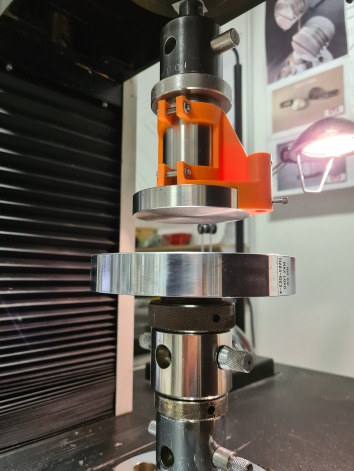
Figure 4: Instron® 4502 dynamometer used for the ground truth test of the specimens.

The tests were performed on parallelepiped-shaped specimens (see Figure 5) with $50\times 50$ mm section and thickness in range $20-30$ mm, at a cross-head speed of $50$ mm/min with sampling rate of $25$ pt/s (or $25$ Hz) up to $5$ mm of compression.

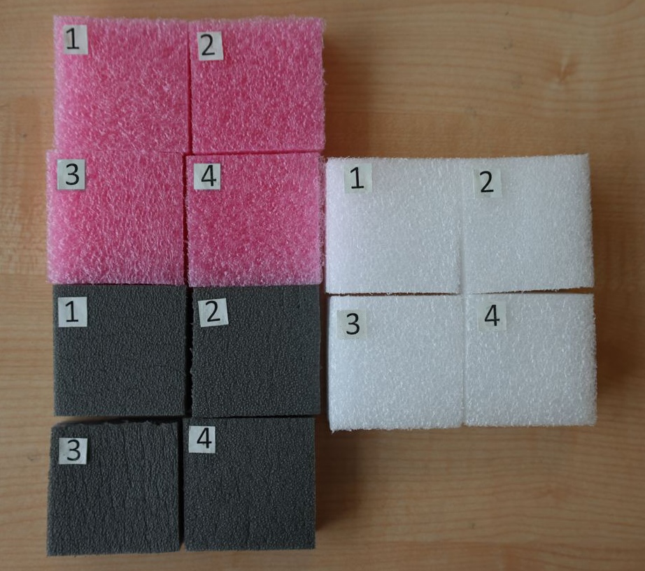
Figure 5: Specimens used during the experiments made of multilayer polymeric foams.

The samples used in the experiments were polymeric foams made of polyethylene and formed from multiple layers to achieve the desired thickness for the experiments, which present elasticity values comparable with biological tissues [19]. The geometric and physical characteristics are specified in Table I.

TABLE I: Geometric and physical parameters of the specimens.

Specimen	Density [$\text{\,}\mathrm{g}\mathrm{/}\mathrm{c}\mathrm{m}^{3}$]	Length x Width x Height [$\text{\,}\mathrm{m}\mathrm{m}^{3}$]
White	$0.0350$	$50\times 50\times 30$
Pink	$0.0181$	$50\times 50\times 20$
Grey	$0.0236$	$50\times 50\times 20$

III-A Robotic system

The robot that has been used for the experiment is an Ur3e, a widely used collaborative industrial robot. It has a maximum payload of $3$ kg and a pose repeatability per ISO 9283 of $\pm 0.03$ mm. Since the Ur3e is a $6$ degree-of-freedom robotic arm, we have $m=6$ in (12). At the end-effector of the manipulator is attached a $6$-axis force-torque sensor, i.e., the BOTA System SensONE. The sensor works at $800$ Hz with a peak-to-peak standard uncertainty of $48\cdot 10^{-3}$ N in the $z$-direction. Attached to the sensor there is a 3D printed indenter, whose position is computed using the $m$ joint encoders measurements. The robotic arm is controlled by a simple motion controller in the Cartesian space. This means that given the Cartesian position of the end-effector as input, the values of the joints are calculated by the robot inverse kinematics. The convergence speed is controlled by a PD controller, were the proportional gain was empirically set to $20$, while the derivative gain to $0.5$, thus ensuring an end-effector trajectory following with negligible errors.

III-B Results and analysis

The tests carried out with the laboratory instrument in Figure 5, treated here as ground truth, have been repeated using the Ur3e manipulator. The experiments were conducted using three different tips: a flat tip with $1$ cm radius, a spherical tip with $1$ cm radius and a parabolic tip with $1.17$ cm radius, all depicted in Figure 6.

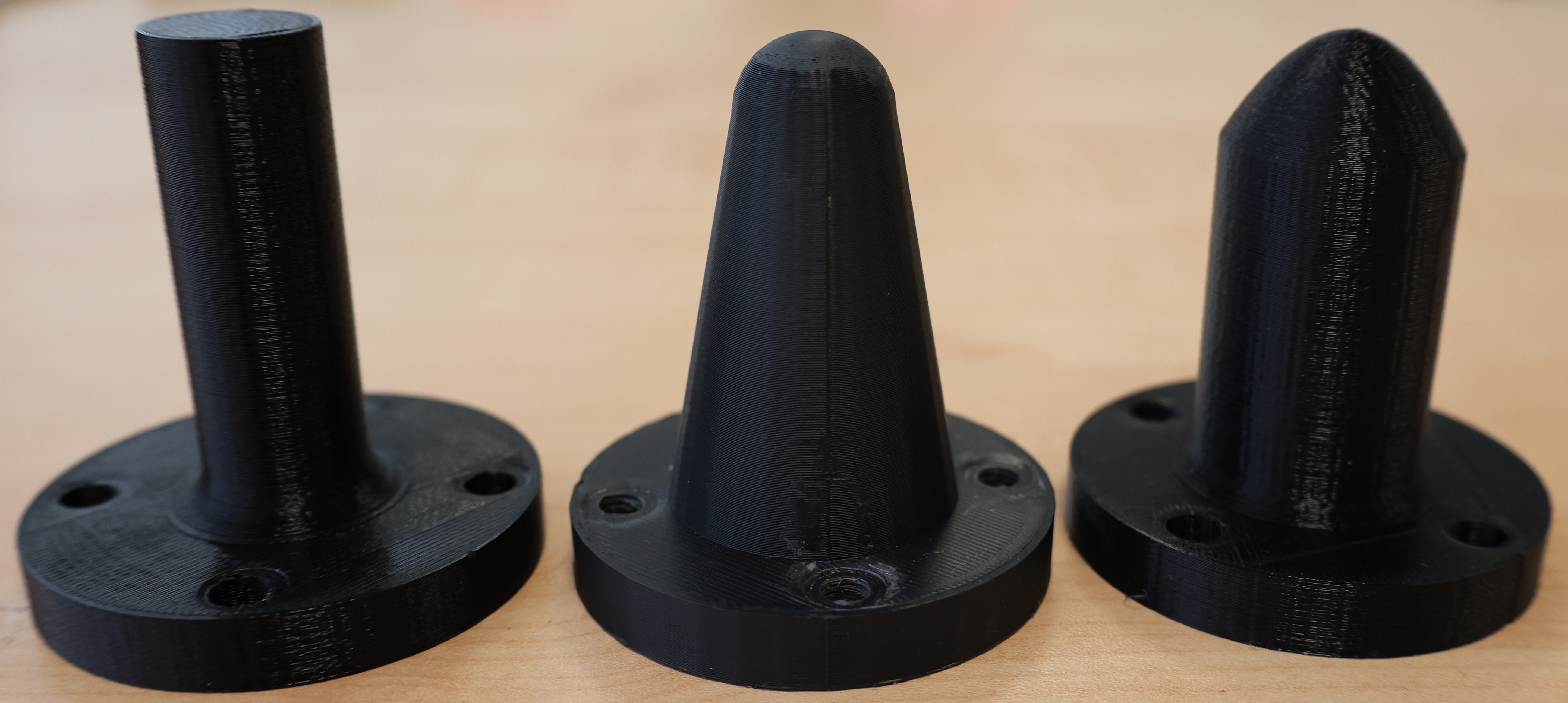
Figure 6: 3D-printed tips utilised in the experiments. From left: the flat, the spherical and the parabolic tips.

For comparisons, the penetration velocity remained consistent at $50$ mm per minute, as in the laboratory test. The indentation depth is adjusted to $10\%$ of the sample thickness to remain within the range of material linearity [18, 21], since any deeper penetration could amplify the non-linear characteristics of the material that are not modelled. During the experiment, the position and force in the $z$-direction are collected for the following offline post-processing, as described in Figure 3. Using (15), we were able to reconstruct the force quite precisely with a mean residual value that never exceeded $0.03\text{\,}\mathrm{k}\mathrm{Pa}^{2}$ for the spherical and paraboloidal tip and $0.06\text{\,}\mathrm{k}\mathrm{Pa}^{2}$ for the flat tip, as can be seen in Table II.

TABLE II: Residual resulting from the force reconstruction $\left[$\text{\,}\mathrm{k}\mathrm{Pa}^{2}$\right]$.

Specimen	Flat Tip	Sphere Tip	Paraboloid Tip
White	0.0316	0.0240	0.0292
Pink	0.0225	0.0250	0.0291
Grey	0.0613	0.0208	0.0308

The position of the surface for each specimen was estimated with relatively high accuracy except for the flat tip, resulting in a mean error for the spherical and paraboloidal tip of $0.38$ mm and for $0.39$ mm, respectively. Instead, since the flat tip had non-linearity of the phase after contact, we used the force measurements after $20\%$ of penetration to estimate the specimen elasticity. The estimated elasticity quantities are consistent with the ground truth, as depicted in Table III.

TABLE III: Results of the elastic value estimations for three different specimens using the three tips represented with the elasticity estimates $E$, the standard uncertainty $\sigma$, and the relative error $err$ with respect to the ground truth.

The flat tip exhibits the poorest behaviour due to the previously mentioned issues, leading to a maximum relative error of nearly $20\%$. On the other hand, the estimates for the spherical and the paraboloidal tip have a maximum relative error of $10\%$. Notice that the standard uncertainty of the ground truth is almost entirely due to the slight differences of the tested samples of the same material: a variability of up to $10\%$ may be expected due to the intricate structure of the expanded foam characteristics [22], since the average pore size significantly affects the mechanical properties and can differ among specimens. However, an uncertainty of $10\%$ is more than acceptable for medical applications given that cancers can be up to $100$ times stiffer than normal soft tissue [23].

The error between the ground truth forces and the one derived from the adopted models are reported in Figure 7.

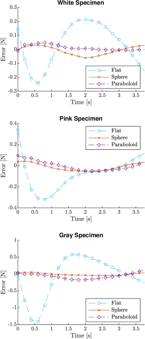
Figure 7: Average force error between the measured and the estimated value in the three specimens. In all experiments, the average error using the spherical and the paraboloid indenter is bounded, demonstrating the suitability of the model with these indenter shapes. On the other hand, the oscillating average error of the flat indenter does not ensure precise force estimation.

Again, the spherical and paraboloidal tips accurately reconstruct the forces along the contact, while the model with a flat surface shows less accuracy that maybe requires a nonlinear model to accurately describe the contact between the flat tip and the specimens.

As materials such as expanded foams require time to recover their characteristics after a test, we aim to investigate whether multiple measurements can be taken in a short time frame while accurately estimating the elasticity value. So we tried to understand if the increase in the material stiffness that occurs in foams when they are not allowed to restore to their initial properties after excitation was measurable by our system. Figure 8 illustrates how the elasticity changes with an increase in the palpation/excitation frequency.

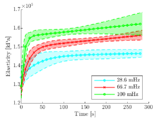
Figure 8: Change in stiffness when multiple experiments are performed without letting the specimen recover its characteristics. Each curve has its confidence interval of $95\%$.

When excitations had higher frequencies (i.e., there is less time for recovery from the previous deformation), higher measured elasticities are observed. This phenomenon can be mathematically modelled as a sum of two exponential functions:

$$E(t)=c_{1}e^{c_{2}t}+c_{3}e^{c_{4}t},$$ (16)

where $t$ us the time passed after the excitation, $c_{i}$ are tuning constants and $E(t)$ the elasticity. It can be seen from Figure 8 that the designed instrument is able to also detect this subtle changes in the material elasticity, thus it can be applied to estimate the parameters of (16) and, more importantly, further proving that our system is suitable for the foreseen medical applications.

IV Conclusion

In this paper, we have an experimental setup, based on the use of a robotic device, to estimate the elastic parameter of a material. This is fundamental to the development of robotic medical applications based on the physical interaction between a probe and the patient’s body. The paper shows that it is possible to reconstruct the contact force with high precision using different types of tips. By leveraging these results, we could estimate the elasticity value with an accuracy that is sufficient to detect imperfections in the human tissues that could reveal the presence of possible diseases.

Further work is required to improve the method. It is not reasonable to assume that all actions performed by the robot will be quasi-static and, hence, it will be necessary to implement a component that considers the dynamic properties of the material. In addition, an online estimation algorithm would be invaluable for automated diagnostic applications based on precise tactile inspections of some parts of the human body. In this paper, we have set the basis for this future development showing the high degree of accuracy that these measurements can potentially reach.

References

- [1] X. Zhu, B. Gao, Y. Zhong, C. Gu, and K. S. Choi, “Extended Kalman filter for online soft tissue characterization based on Hunt-Crossley contact model,” Journal of the Mechanical Behavior of Biomedical Materials, vol. 123, 2021.
- [2] A. Haddadi and K. Hashtrudi-Zaad, “Real-time identification of hunt-crossley dynamic models of contact environments,” IEEE Transactions on Robotics, vol. 28, no. 3, pp. 555–566, 2012.
- [3] A. Pappalardo, A. Albakri, C. Liu, L. Bascetta, E. De Momi, and P. Poignet, “Hunt-Crossley model based force control for minimally invasive robotic surgery,” Biomedical Signal Processing and Control, vol. 29, 2016.
- [4] J. F. Greenleaf, M. Fatemi, and M. Insana, “Selected methods for imaging elastic properties of biological tissues,” 2003.
- [5] H. P. Dobrev, “In vivo study of skin mechanical properties in patients with systemic sclerosis,” Journal of the American Academy of Dermatology, vol. 40, no. 3, 1999.
- [6] A. Lau, M. L. Oyen, R. W. Kent, D. Murakami, and T. Torigaki, “Indentation stiffness of aging human costal cartilage,” Acta Biomaterialia, vol. 4, no. 1, 2008.
- [7] A. Tang, G. Cloutier, N. M. Szeverenyi, and C. B. Sirlin, “Ultrasound elastography and MR elastography for assessing liver fibrosis: Part 1, principles and techniques,” American Journal of Roentgenology, vol. 205, no. 1, 2015.
- [8] A. Manduca, P. V. Bayly, R. L. Ehman, A. Kolipaka, T. J. Royston, I. Sack, R. Sinkus, and B. E. Van Beers, “MR elastography: Principles, guidelines, and terminology,” 2021.
- [9] N. Frulio and H. Trillaud, “Ultrasound elastography in liver,” 2013.
- [10] G. Y. Li and Y. Cao, “Mechanics of ultrasound elastography,” 2017.
- [11] K. Kumar, M. E. Andrews, V. Jayashankar, A. K. Mishra, and S. Suresh, “Measurement of viscoelastic properties of polyacrylamide-based tissue-mimicking phantoms for ultrasound elastography applications,” in IEEE Transactions on Instrumentation and Measurement, vol. 59, no. 5, 2010.
- [12] A. Eder, T. Arnold, and C. Kargel, “Performance evaluation of displacement estimators for real-time ultrasonic strain and blood flow imaging with improved spatial resolution,” IEEE Transactions on Instrumentation and Measurement, vol. 56, no. 4, 2007.
- [13] V. L. Popov and M. Heß, Method of dimensionality reduction in contact mechanics and friction. Springer, 2015.
- [14] K. L. Johnson, Contact mechanics. Cambridge University Press, 1985.
- [15] W. C. Hayes, L. M. Keer, G. Herrmann, and L. F. Mockros, “A mathematical analysis for indentation tests of articular cartilage,” Journal of Biomechanics, vol. 5, no. 5, 1972.
- [16] M. Sakamoto, G. Li, T. Hara, and E. Y. Chao, “A new method for theoretical analysis of static indentation test,” Journal of Biomechanics, vol. 29, no. 5, 1996.
- [17] N. E. Waters, “The indentation of thin rubber sheets by cylindrical indentors,” British Journal of Applied Physics, vol. 16, no. 9, 1965.
- [18] E. K. Dimitriadis, F. Horkay, J. Maresca, B. Kachar, and R. S. Chadwick, “Determination of elastic moduli of thin layers of soft material using the atomic force microscope,” Biophysical Journal, vol. 82, no. 5, 2002.
- [19] P. N. Wells and H. D. Liang, “Medical ultrasound: imaging of soft tissue strain and elasticity,” Journal of The Royal Society Interface, vol. 8, no. 64, pp. 1521–1549, 11 2011. [Online]. Available: https://royalsocietypublishing.org/doi/10.1098/rsif.2011.0054
- [20] J. J. Uigker, J. Denavit, and R. S. Hartenberg, “An iterative method for the displacement analysis of spatial mechanisms,” Journal of Applied Mechanics, Transactions ASME, vol. 31, no. 2, 1964.
- [21] B. Qiang, J. Greenleaf, M. Oyen, and X. Zhang, “Estimating material elasticity by spherical indentation load-relaxation tests on viscoelastic samples of finite thickness,” IEEE Transactions on Ultrasonics, Ferroelectrics, and Frequency Control, vol. 58, no. 7, 2011.
- [22] O. Weißenborn, S. Geller, M. Gude, F. Post, S. Praetorius, A. Voigt, and S. Aland, “Deformation analysis of polymer foams under compression load using in situ computed tomography and finite element simulation methods,” in ECCM 2016 - Proceeding of the 17th European Conference on Composite Materials, 2016.
- [23] R. Nadan, H. Irena, O. Milorad, O. Rajko, J. R. Jasminka, K. Marino, P. Roland, and V. Boris, “EUS elastography in the diagnosis of focal liver lesions,” Gastrointestinal Endoscopy, vol. 66, no. 4, 2007.