Matching prior pairs
connecting Maximum A Posteriori estimation
and posterior expectation

Abstract

Bayesian statistics has two common measures of central tendency of a posterior distribution: posterior means and Maximum A Posteriori (MAP) estimates. In this paper, we discuss a connection between MAP estimates and posterior means. We derive an asymptotic condition for a pair of prior densities under which the posterior mean based on one prior coincides with the MAP estimate based on the other prior. A sufficient condition for the existence of this prior pair relates to $\alpha$-flatness of the statistical model in information geometry. We also construct a matching prior pair using $\alpha$-parallel priors. Our result elucidates an interesting connection between regularization in generalized linear regression models and posterior expectation.

and

1 Introduction

In Bayesian statistics, two common measures of central tendency of a posterior distribution are posterior mean and Maximum A Posteriori (MAP) estimate. Posterior mean is the Bayes estimate, an estimate minimizing the expected loss for a squared-error loss function. This is usually computed by the expectation using Markov chain Monte Carlo (MCMC). MAP estimate lies in the literature of penalized likelihood estimate or regularized maximum likelihood estimate. This is obtained by the optimization. Although the computational schemes of two estimates are different, the celebrated Bernstein–von-Mises theorem tells that in the first-order asymptotic regime of the sample size, the posterior shape becomes Gaussian with the center equal to the MAP estimate. Thus the posterior mean and the MAP estimate become the same in the asymptotic regime. Yet, practical behaviours of these estimates are quite different (e.g., Pananos and Lizotte, 2020). Recent studies (Gribonval, 2011; Gribonval and Machart, 2013; Louchet and Moisan, 2013; Burger and Lucka, 2014) highlight differences and connections between these estimates in several statistical models. In particular, Gribonval and Machart (2013) reveals that in Gaussian linear inverse problems, although the posterior mean and the MAP estimate for the same prior may be different, every posterior mean based on a prior is also the MAP estimate based on a different prior.

To elucidate a further connection between MAP estimates and posterior means in general statistical models, this paper derives the asymptotic condition for a pair of priors $(\pi,\widetilde{\pi})$ under which the posterior mean derived from one prior $\pi$ coincides with the MAP estimate based on the other prior $\widetilde{\pi}$. We call this pair of priors matching prior pair. From our discovery of matching prior pairs, we see that in a generalized linear regression model, although the posterior mean based on a Gaussian prior may be different from the ridge regression (the MAP estimate based on a Gaussian prior), the matching prior pair of the Gaussian prior can deliver the MAP estimate closer to the posterior mean based on the Gaussian prior in asymptotic regimes. The discovery also has practical implications, in particular, in the computation of each estimate. When there exists a difficulty in optimizing the log posterior density to obtain a MAP estimate for a prior, we can utilize the posterior mean based on another prior that forms a matching pair with the given prior. In contrast, when it is hard to build an MCMC for computing a posterior mean, we can instead evaluate a MAP estimate that matches to the posterior mean.

The existence of a matching prior pair has an information-geometrical flavor (Amari, 1985). The information geometry presents a class of $\alpha$-connections $(\alpha\in\mathbb{R})$ concerning the manifold of probability distributions. We show that a matching prior pair exists if the target statistical model is $\alpha$-flat and the target parameter is $\alpha$-affine for some $\alpha\in\mathbb{R}$. Further, we also provide an explicit construction of the matching prior pair using $\alpha$-parallel priors (Takeuchi and Amari, 2005). This information-geometrical notation appears because the posterior expectation elicits the information about the flatness of the statistical model with respect to the $(-1)$-connection as observed in Komaki (1996) and in Okudo and Komaki (2021).

There is a literature on bridging the gap between the MAP estimation and the posterior expectation. In the objective Bayesian literature, a prior yielding the posterior mean asymptotically equal to the maximum likelihood estimate (MLE) is called by the moment matching prior. Ghosh and Liu (2011) derives a formula for constructing a moment matching prior. Hashimoto (2019) extends the construction to non-regular statistical models. Yanagimoto and Miyata (2023) extends the moment matching prior to the conditional inference. Our matching prior pair includes the moment matching prior and naturally extends its idea to the MAP estimate based on a non-uniform distribution. Gribonval and Machart (2013) reveals an elegant construction of an exact matching prior pair for linear inverse problems. Polson and Scott (2016) proposes an exact prior pair that matches a density with a MAP estimate plugged-in and a marginal density. These results are exact in the sense that it holds even in the finite regime of sample size but are limited to several models. Although our construction relies on the asymptotics with respect to the sample size, it elucidates the connection in general statistical models using information geometry.

The rest of this paper is structured as follows. Section 2 delivers the main result, an information-geometrical construction of a matching prior pair. Section 2.3 displays analytical examples that examine the main result. Section 3 presents numerical examples using synthetic and real data. All technical proofs are presented in Section 4.

2 Matching prior pairs

We first prepare several notations for the theory and then present the construction of the matching prior pair.

2.1 Preparation

Let $\mathcal{Y}$ be a sample space and let $dy$ be a base measure. Assume that we have observations $y^{n}=\{y(1),y(2),\dots,y(n)\}~{}~{}(y(1),\dots,y(n)\in\mathcal{Y})$ independently distributed according to a probability distribution with a density function $p(y\,;\,\theta)$ that belongs to a statistical model parameterized by $\theta$:

$$\mathcal{P}=\left\{p(y\,;\,\theta)\mid\theta\in\Theta\right\}\,\,\text{with}\,\,\Theta\subset\mathbb{R}^{d}.$$

We denote by $\mathrm{E}_{\theta}$ the expectation with respect to the density with $\theta$.

For the theory, we first introduce several information-geometric notations; for details, see Amari (1985). Components of the Fisher information matrix $g=(g_{ab})_{a,b=1,\ldots,d}$ are defined as

$$g_{ab}(\theta):=\int p(y\,;\,\theta)\{\partial_{a}\log p(y\,;\,\theta)\}\{\partial_{b}\log p(y\,;\,\theta)\}dy=\int\frac{\partial_{a}p(y\,;\,\theta)\partial_{b}p(y\,;\,\theta)}{p(y\,;\,\theta)}dy$$

where $\partial_{a}=\partial/\partial\theta^{a}$. For $a,b=1,\ldots,d$, let $g^{ab}$ be a component of the inverse matrix of the Fisher information matrix $g$. For $a,b,c=1,\ldots,d$, the m-connection coefficient (the $(-1)$-connection coefficient) and e-connection coefficient (the $1$-connection coefficient) are defined as

$$\raise 1.5pt\hbox{$\displaystyle\mathop{\Gamma}^{\rm m}$}_{abc}^{\,}:=\int\frac{\partial_{a}\partial_{b}p(y\,;\,\theta)\partial_{c}p(y\,;\,\theta)}{p(y\,;\,\theta)}dy\mbox{~{}~{}and~{}~{}}\raise 1.5pt\hbox{$\displaystyle\mathop{\Gamma}^{\rm e}$}_{abc}^{\,}:=\int p(y;\theta)\{\partial_{a}\partial_{b}\log p(y\,;\,\theta)\}\{\partial_{c}\log p(y\,;\,\theta)\}dy,$$ (1)

respectively. For $a,b,c=1,\ldots,d$, let

$$T_{abc}:=\raise 1.5pt\hbox{$\displaystyle\mathop{\Gamma}^{\rm m}$}_{abc}^{\,}-\raise 1.5pt\hbox{$\displaystyle\mathop{\Gamma}^{\rm e}$}_{abc}^{\,}=\int p(y;\theta)\{\partial_{a}\log p(y\,;\,\theta)\}\{\partial_{b}\log p(y\,;\,\theta)\}\{\partial_{c}\log p(y\,;\,\theta)\}dy.$$

Further, the $\alpha$-connection coefficient for $\alpha\in\mathbb{R}$ is defined as

$$\raise 1.5pt\hbox{$\displaystyle\mathop{\Gamma}^{\alpha}$}_{abc}^{\,}:=\raise 1.5pt\hbox{$\displaystyle\mathop{\Gamma}^{\rm m}$}_{abc}^{\,}-\frac{1+\alpha}{2}T_{abc}=\raise 1.5pt\hbox{$\displaystyle\mathop{\Gamma}^{\rm e}$}_{abc}^{\,}+\frac{1-\alpha}{2}T_{abc}\,\,\,(a,b,c=1,\ldots,d).$$ (2)

These connections form dual connections, that is,

$$\partial_{a}g_{bc}(\theta)=\raise 1.5pt\hbox{$\displaystyle\mathop{\Gamma}^{\alpha}$}_{abc}^{\,}(\theta)+\raise 1.5pt\hbox{$\displaystyle\mathop{\Gamma}^{-\alpha}$}_{acb}^{\,}(\theta)\quad\text{for any}\,\,\alpha\in\mathbb{R}.$$ (3)

To ease the notation, we use the Einstein summation convention: if an index occurs twice in any one term, once as an upper and once as a lower index, summation over that index is implied. Let

$$T_{a}:=T_{abc}g^{bc}\quad\text{and}\quad\raise 1.5pt\hbox{$\displaystyle\mathop{\Gamma}^{\alpha}$}_{ab}^{\,~{}c}:=\raise 1.5pt\hbox{$\displaystyle\mathop{\Gamma}^{\alpha}$}_{abe}^{\,}g^{ce}\,\,\,\,\text{for}\,\,a,b,c=1,\ldots,d.$$

We then prepare notions of flatness in the information geometry. For given $\alpha\in\mathbb{R}$, the statistical model $\mathcal{P}$ is called $\alpha$-flat if and only if there exists a parameterization with $\raise 1.5pt\hbox{$\displaystyle\mathop{\Gamma}^{\alpha}$}_{abc}^{\,}=0$ for all $a,b,c=1,\ldots,d$; e.g., p.47 of Amari (1985). The parameterization with $\raise 1.5pt\hbox{$\displaystyle\mathop{\Gamma}^{\rm m}$}_{abc}^{\,}=0$ for $a,b,c=1,\ldots,d$ is called an $\alpha$-affine coordinate. Further, the statistical model is said to be statistically equi-affine when $\partial_{a}T_{b}=\partial_{b}T_{a}$ for $\theta\in\Theta$; e.g., Definition 2 of Takeuchi and Amari (2005). The concept of statistical equi-affinity is important to the existence of the subsequent $\alpha$-parallel priors and we have a handy sufficient condition for the statistically equi-affinity as described below.

Lemma 2.1 (Lauritzen (1987); Propositions 3 and 4 of Takeuchi and Amari (2005)).

If the model is $\alpha$-flat for a certain $\alpha\neq 0$, it is statistically equi-affine.

We thirdly introduce $\alpha$-parallel priors. For $\alpha\in\mathbb{R}$, an $\alpha$-parallel prior $\pi_{\alpha}$ proposed by Takeuchi and Amari (2005) is defined by

$$\partial_{a}\log\pi_{\alpha}(\theta)=\raise 1.5pt\hbox{$\displaystyle\mathop{\Gamma}^{\alpha}$}_{ab}^{\,~{}b}(\theta)\,\,\,(a=1,\ldots,d)$$ (4)

if it exists. This class contains several non-informative priors proposed in the objective Bayesian literature (e.g., Tanaka, 2023). First, it includes the well-known Jeffreys prior $\pi_{\mathrm{J}}(\theta):=|g(\theta)|^{1/2}$ with the determinant $|\cdot|$ as the $0$-parallel prior:

$$\partial_{a}\log\pi_{\rm J}(\theta)=\frac{1}{2}\partial_{a}\log|g|(\theta)=\frac{1}{2}g^{bc}(\theta)\partial_{a}g_{bc}(\theta)=\raise 1.5pt\hbox{$\displaystyle\mathop{\Gamma}^{0}$}_{ab}^{\,~{}b}(\theta)\,\,\,(a=1,\ldots,d).$$

Second, it has the $\chi^{2}$-prior $\pi_{\chi^{2}}(\theta)$ proposed by Liu et al. (2014) as $1/2$-parallel prior:

$$\partial_{a}\log\pi_{\chi^{2}}(\theta)=\raise 1.5pt\hbox{$\displaystyle\mathop{\Gamma}^{1/2}$}_{ab}^{\,~{}b}(\theta)\,\,\,(a=1,\ldots,d),$$

which is recently pointed out by Tanaka (2023). For $\alpha=1$, we call this e-parallel prior $\pi_{\rm e}$, and for $\alpha=-1$, we call this m-parallel prior $\pi_{\rm m}$. Takeuchi and Amari (2005) find the following lemmas for the existence of $\alpha$-parallel priors.

Lemma 2.2 (Proposition 2 of Takeuchi and Amari (2005)).

A statistically equi-affine statistical model has $\alpha$-parallel priors for any $\alpha\in\mathbb{R}$. Otherwise, the model has only the $0$-parallel prior.

Lemma 2.3 (Proposition 5 of Takeuchi and Amari (2005)).

If a statistical model is $\alpha_{0}$-flat for a certain $\alpha_{0}\neq 0$, then the model has $\alpha$-parallel priors for arbitrary $\alpha\in\mathbb{R}$.

Example 2.1 (Exponential family).

Consider an exponential family with a sufficient statistic $T(y)\in\mathbb{R}^{d}$:

$$\{\,\exp\{\theta^{\top}T(y)-\psi(\theta)\}m(y)\mid\theta\in\Theta\},$$

where $\psi(\theta)$ is the potential function and $m(y)$ is a given function. The exponential family is $\mathrm{e}$- & $\mathrm{m}$-flat ($\pm 1$-flat), that is, it has parameterizations $\theta$ and $\eta=\mathrm{E}_{\theta}[T(Y)]$ with $\raise 1.5pt\hbox{$\displaystyle\mathop{\Gamma}^{\rm e}$}_{ab}^{\,~{}c}(\theta)=0$ and $\raise 1.5pt\hbox{$\displaystyle\mathop{\Gamma}^{\rm m}$}_{ab}^{\,~{}c}(\eta)=0$, respectively. Thus, Lemma 2.3 implies that exponential families have $\alpha$-parallel priors for arbitrary $\alpha$. In particular, the $\mathrm{e}$-parallel prior is a uniform prior with respect to $\theta$, and the $\mathrm{m}$-parallel prior is a uniform prior with respect to $\eta$.

We conclude this subsection by introducing a condition on the existence of the solution of a certain partial differential equation. For a differentiable function $h(\theta)=(h_{1}(\theta),\ldots,h_{d}(\theta))^{\top}$, consider the partial differential equation of $u(\theta)$ given by

$$\partial_{a}u(\theta)=h_{a}(\theta)\quad(a=1,\ldots,d).$$

Lemma 2.4 (p. 348 of Zwillinger (1997); Section 1-3 of Matsuda (1976)).

If $\partial_{b}h_{a}(\theta)=\partial_{a}h_{b}(\theta)$ for $1\leq a<b\leq d$, then $u(\theta)$ exists locally.

2.2 Main results

We present information-geometrical condition and construction of matching prior pairs. We begin with an asymptotic condition of matching prior pairs for general models, and then we derive a simple form for $\alpha$-flat statistical models and $\alpha$-affine parametrization. Lastly, we derive matching prior pairs for other statistics including variance and higher-order moments. In the rest of the paper, we assume the regularity conditions in Hartigan (1998).

The following theorem delivers an asymptotic condition to match a posterior mean based on a prior $\pi_{\mathrm{PM}}$ and a MAP estimate based on a prior $\pi_{\mathrm{MAP}}$ except for terms of ${\rm o}_{p}(n^{-1})$. The proof is given in Section 4.

Theorem 2.1.

The posterior mean $\hat{\theta}_{\rm PM}$ based on a prior $\pi_{\rm PM}$ and the MAP estimate $\hat{\theta}_{\rm MAP}$ based on a prior $\pi_{\rm MAP}$ coincide except for terms of $o_{p}(n^{-1})$ when the prior pair $(\pi_{\mathrm{PM}},\pi_{\mathrm{MAP}})$ satisfies, for $a=1,\ldots,d$,

$$\partial_{a}\log\frac{\pi_{\rm PM}}{\pi_{\rm MAP}}(\hat{\theta}_{\rm MLE})-\left(\partial_{a}\log\pi_{\rm J}(\hat{\theta}_{\rm MLE})+\frac{1}{2}g^{cd}(\hat{\theta}_{\rm MLE})\raise 1.5pt\hbox{$\displaystyle\mathop{\Gamma}^{\rm e}$}_{cda}^{\,}(\hat{\theta}_{\rm MLE})\right)=\mathrm{o}_{p}(n^{-1}),$$ (5)

where $\hat{\theta}_{\rm MLE}$ is the MLE.

Remark 2.1.

Theorem 2.1 includes the construction of the moment matching prior proposed by Ghosh and Liu (2011). The moment matching prior is the prior that yields the posterior mean asymptotically equal to the MLE. Tanaka (2023) rewrites the partial differential equation for the moment matching prior $\pi_{\rm MM}$ in an information-geometrical way:

$$\partial_{a}\log\pi_{\rm MM}(\theta)-\left(\partial_{a}\log{\pi_{\rm J}}(\theta)+\frac{1}{2}g^{cd}(\theta)\raise 1.5pt\hbox{$\displaystyle\mathop{\Gamma}^{\rm e}$}_{cda}^{\,}(\theta)\right)=0\,\,\,(a=1,\ldots,d).$$

As the prior that yields MLE as the MAP estimate is a uniform prior, the moment matching prior $\pi_{\rm MM}$ satisfies (5) as the matching prior pair of a uniform prior.

Remark 2.2.

Equation 5 lacks the invariance with respect to parameterization, which implies that an explicit form of a matching prior pair depends on parameterization. This is reasonable because the forms of both the posterior mean and the MAP estimate change according to the parameterization.

In a one-dimensional statistical model, an explicit construction of a matching prior pair is easy. Consider the following ordinary differential equation:

$$\frac{d}{d\theta}\log\frac{\pi_{\rm PM}(\theta)}{\pi_{\rm MAP}(\theta)\pi_{\rm J}(\theta)}=\frac{1}{2}g^{11}(\theta)\raise 1.5pt\hbox{$\displaystyle\mathop{\Gamma}^{\rm e}$}_{111}^{\,}(\theta).$$

The integration with respect to $\theta$ yields, for arbitrary $\theta_{0}\in\Theta$,

$$\frac{\pi_{\rm PM}(\theta)}{\pi_{\rm MAP}(\theta)}\propto\pi_{\rm J}(\theta)\exp\left\{\int_{\theta_{0}}^{\theta}\left(\frac{1}{2}g^{11}(\theta^{\prime})\raise 1.5pt\hbox{$\displaystyle\mathop{\Gamma}^{\rm e}$}_{111}^{\,}(\theta^{\prime})d\theta^{\prime}\right)\right\}.$$

Yet, in a multi-dimensional statistical model, even the existence of a matching prior pair is non-trivial. We then seek a sufficient condition for the existence of a matching prior pair and an explicit construction of the pair. The following corollary provides a sufficient condition of the existence and a explicit construction using information geometry.

Corollary 2.1.

Assume that the model is $\alpha$-flat and $\theta$ is $\alpha$-affine for a certain $\alpha\neq 0$. Then, a matching prior pair exists. Further, the prior pair $(\pi_{\rm PM},\pi_{\rm MAP})$ satisfying

$$\frac{\pi_{\rm PM}(\theta)}{\pi_{\rm MAP}(\theta)}\propto\pi_{\rm J}(\theta)\left(\frac{\pi_{\rm e}(\theta)}{\pi_{\rm m}(\theta)}\right)^{(1-\alpha)/4}$$ (6)

is a matching prior pair; that is, the posterior mean based on $\pi_{\rm PM}$ and the MAP estimate based on $\pi_{\rm MAP}$ coincide except for terms of $o_{p}(n^{-1})$.

Proof.

Observe that we have $\raise 1.5pt\hbox{$\displaystyle\mathop{\Gamma}^{\rm e}$}_{abc}^{\,}(\theta)=-\{(1-\alpha)/2\}T_{abc}(\theta)$ ($a,b,c=1,\ldots,d$) for an $\alpha$-affine coordinate $\theta$. Together with (2), this implies that for an $\alpha$-affine coordinate $\theta$, the condition (5) becomes

$$\partial_{a}\left(\log\frac{\pi_{\rm PM}(\theta)}{\pi_{\rm MAP}(\theta)\pi_{\rm J}(\theta)}\right)=-\frac{1-\alpha}{4}T_{a}(\theta)+{\rm o}_{p}(n^{-1})\quad\text{for $\theta=\hat{\theta}_{\rm MLE}$}.$$

Then, consider the following partial differential equation:

$$\partial_{a}\left(\log\frac{\pi_{\rm PM}(\theta)}{\pi_{\rm MAP}(\theta)\pi_{\rm J}(\theta)}\right)=-\frac{1-\alpha}{4}T_{a}(\theta).$$ (7)

Lemma 2.4 tells that this equation has a solution if

$$\partial_{b}T_{a}(\theta)=\partial_{a}T_{b}(\theta)\quad(1\leq a<b\leq d),$$

which is equal to the statistical equi-affinity of the model. An $\alpha$-flat model satisfies the equi-affinity (Lemma 2.3) and thus a matching prior pair exists.

Further, by the definition of the e-&m-parallel priors (4), we have

$$\partial_{a}\log\frac{\pi_{\rm m}(\theta)}{\pi_{\rm e}(\theta)}=T_{a}(\theta)\,\,\,(a=1,\ldots,d),$$

and obtain

$$\partial_{a}\left(\log\frac{\pi_{\rm PM}(\theta)}{\pi_{\rm MAP}(\theta)\pi_{\rm J}(\theta)}\right)=\partial_{a}\log\left(\frac{\pi_{\rm e}(\theta)}{\pi_{\rm m}(\theta)}\right)^{(1-\alpha)/4}\quad(a=1,\ldots,d).$$

So, the prior pair (6) is a matching prior pair, which completes the proof. ∎

We shall give several examples in the following subsection. We conclude this section with the following extension of matching prior pairs, that is, matching prior pairs for other statistics including higher-order moments.

Proposition 2.1.

Let $f(\theta)=(f_{1}(\theta),\ldots,f_{d}(\theta))$ be a third-times differentiable function. If two priors $\pi_{\rm PM}$ and $\pi_{\rm MAP}$ satisfy

$$\partial_{a}f_{i}(\theta)\left\{\partial_{b}\log\frac{\pi_{\rm PM}}{\pi_{\rm MAP}}(\theta)-\partial_{b}\log\pi_{\rm J}(\theta)-\frac{1}{2}g^{cd}(\theta)\raise 1.5pt\hbox{$\displaystyle\mathop{\Gamma}^{\rm e}$}_{cdb}^{\,}(\theta)\right\}-\frac{1}{2}\partial_{a}\partial_{b}f_{i}(\theta)=\mathrm{o}_{p}(n^{-1})$$

at $\theta=\hat{\theta}_{\rm MLE}$ for $i=1,\ldots,d$ and $a=1,\ldots,d$, the posterior expectation $f_{\pi_{\rm PM}}$ of $f$ based on $\pi_{\rm PM}$ and the MAP-plugged-in estimate $f(\hat{\theta}_{\rm MAP})$ based on $\pi_{\rm MAP}$ coincide except for $\mathrm{o}_{p}(n^{-1})$-terms.

2.3 Examples

In this section, we present matching prior pairs (6) in a submodel of an exponential family:

$$\{\exp\{\theta^{\top}(\xi)T(y)-\psi(\theta(\xi))\}m(y)\mid\xi\in\Xi\},$$

where $\theta$ is the $p$-dimensional canonical/natural parameter of the exponential family, and $\xi$ is a $d$-dimensional model parameter. This includes the exponential family itself and the generalized linear regression model with a canonical link function. As the exponential family is e-&m-flat and has $\alpha$-parallel priors, their e- or m-flat submodels also have $\alpha$-parallel priors and so we confine ourselves to e- or m-flat submodels of an exponential family.

2.3.1 Generalized linear models with canonical links and regression coefficients

We first consider a generalized linear regression model (GLM) with a canonical link function:

$$\{\exp(\theta^{\top}(\beta)T(y)-\psi(\theta(\beta)))m(y)\mid\beta\in\Xi\}\,\,\,\,\text{with}\,\,\theta=X\beta,$$

where $\beta$ is an unknown regression coefficient of $d$ dimension ($p\geq d$), and $X$ is a given full rank matrix $X\in\mathbb{R}^{p\times d}$. In this case, since $\theta$ is the e-affine coordinate and $\partial\theta/\partial\beta=X^{\top}$, the e-connection coefficient with respect to $\beta$ also vanishes $\raise 1.5pt\hbox{$\displaystyle\mathop{\Gamma}^{\rm e}$}_{abc}^{\,}(\beta)=0$, it suffices to seek the prior pair satisfying

$$\partial_{a}\log\frac{\pi_{\rm PM}}{\pi_{\rm MAP}}(\beta)-\left(\partial_{a}\log\pi_{\rm J}(\beta)\right)=0,$$ (8)

which is equal to

$$\frac{\pi_{\rm PM}(\beta)}{\pi_{\rm MAP}(\beta)}\propto\pi_{\rm J}(\beta).$$ (9)

As a simple example, consider a Gaussian model with mean zero and unknown variance: the data $y^{n}=\{y(1),\dots,y(n)\}$ independently come from a Gaussian distribution $N(0,\sigma^{2})$. Here we employ an inverse-gamma prior

$$\sigma^{2}\sim{\rm InvGamma}(a,b)\quad\text{with}\,\,a,b>0.$$

Consider the canonical parameter $\theta=\sigma^{-2}$ and the posterior mean of $\theta$. In this parameterization, the prior becomes

$$\theta\sim{\rm Gamma}(a,b).$$

Let $\pi_{\rm PM}$ denote its density. The posterior distribution of $\theta$ is ${\rm Gamma}(a+n/2,b+\sum\nolimits_{i=1}^{n}y(i)^{2}/2)$, and then the posterior mean based on $\pi_{\rm PM}$ is

$$\hat{\theta}_{\rm PM}=\frac{a+n/2}{b+\sum\nolimits_{i=1}^{n}y(i)^{2}/2}.$$

By using (9), we set $\pi_{\rm MAP}(\theta)\propto\pi_{\rm PM}(\theta)/\pi_{\rm J}(\theta)$, where $\pi_{\rm J}(\theta)\propto\theta^{-1}$. Since the log posterior density based on $\pi_{\rm MAP}$ is

$$\log p(y^{n}\,;\,\theta)+\log\pi_{\rm MAP}(\theta)=\left(a+n/2-1\right)\log\theta-(b+\sum\nolimits_{i=1}^{n}y(i)^{2}/2)\theta+\log\theta+C$$

with the constant $C$ independent from $\theta$, the MAP estimate based on $\pi_{\rm MAP}$ is

$$\hat{\theta}_{\rm MAP}=\frac{a+n/2}{b+\sum\nolimits_{i=1}^{n}y(i)^{2}/2},$$

which implies the exact matching $\hat{\theta}_{\rm PM}=\hat{\theta}_{\rm MAP}$.

2.3.2 m-flat submodels and m-affine parameters

We proceed to a linear submodel with respect to the expectation parameter $\eta=\mathrm{E}_{\theta}[T(Y)]$ of the exponential family:

$$\{\exp(\theta^{\top}(\xi)T(y)-\psi(\theta(\xi)))m(y)\mid\xi\in\Xi\}\,\,\,\,\text{with}\,\,\eta=\eta(\theta)=X\xi,$$

where $\eta\in\mathbb{R}^{p}$, $\xi$ is a model parameter of $d$ dimension $(p\geq d)$, and $X$ is a given full rank matrix $X\in\mathbb{R}^{p\times d}$. In this case, the m-connection coefficients $\raise 1.5pt\hbox{$\displaystyle\mathop{\Gamma}^{\rm m}$}_{abc}^{\,}(\xi)$ ($a,b,c=1,\ldots,d$) vanish and

$$\partial_{a}\log\pi_{\rm J}(\xi)=\raise 1.5pt\hbox{$\displaystyle\mathop{\Gamma}^{0}$}_{ab}^{\,b}(\xi)=\left(\raise 1.5pt\hbox{$\displaystyle\mathop{\Gamma}^{\rm m}$}_{ab}^{\,b}(\xi)-\frac{1}{2}T_{a}(\xi)\right)=-\frac{1}{2}T_{a}(\xi)=-\frac{1}{2}\partial_{a}\log\frac{\pi_{\rm m}(\xi)}{\pi_{\rm e}(\xi)},$$

which implies

$$\frac{\pi_{\rm e}(\xi)}{\pi_{\rm m}(\xi)}\propto\left\{\pi_{\rm J}(\xi)\right\}^{2}.$$

Then, the condition (6) becomes

$$\frac{\pi_{\rm PM}(\xi)}{\pi_{\rm MAP}(\xi)}\propto\pi_{\rm J}(\xi)\left\{(\pi_{\rm J}(\xi))^{2}\right\}^{1/2}=\left\{\pi_{\rm J}(\xi)\right\}^{2}.$$ (10)

As a simple example, consider a Poisson model: the data $y^{n}=\{y(1),\dots,y(n)\}$ independently come from a Poisson distribution ${\rm Poisson}(\lambda)$. Let us consider a Gamma prior $\lambda\sim{\rm Gamma}(a,b)$ with $a,b>0$ for $\lambda$ and denote the density by $\pi_{\rm PM}$. Then the posterior distribution is the Gamma distribution ${\rm Gamma}(a+\sum\nolimits_{i=1}^{n}y(n),b+n)$, and the posterior mean based on $\pi_{\rm PM}$ is

$$\hat{\lambda}_{\rm PM}=\frac{a+\sum\nolimits_{i=1}^{n}y(n)}{b+n}.$$

Since $\lambda$ is the expectation parameter and $\pi_{\rm J}(\lambda)\propto\lambda^{-1/2}$, the matching prior pair satisfies

$$\frac{\pi_{\rm PM}(\lambda)}{\pi_{\rm MAP}(\lambda)}\propto\lambda^{-1}.$$

We set $\pi_{\rm MAP}(\lambda)=\lambda\pi_{\rm PM}(\lambda)$. Since the log posterior density based on $\pi_{\rm MAP}$ is

$$\log p(y^{n}\,;\,\lambda)+\log\pi_{\rm MAP}(\lambda)=\left(a+\sum_{i=1}^{n}y(i)-1\right)\log\lambda-(b+n)\lambda+\log\lambda+C$$

with the constant $C$ independent from $\lambda$, the MAP estimate based on $\pi_{\rm MAP}$ is

$$\hat{\lambda}_{\rm MAP}=\frac{a+\sum\nolimits_{i=1}^{n}y(n)}{b+n},$$

which implies the exact matching $\hat{\lambda}_{\rm PM}=\hat{\lambda}_{\rm MAP}$.

3 Numerical experiments

In this section, we examine the theory using the Bayesian logistic regression model and the Poisson shrinkage model.

3.1 The Bayesian Logistic regression

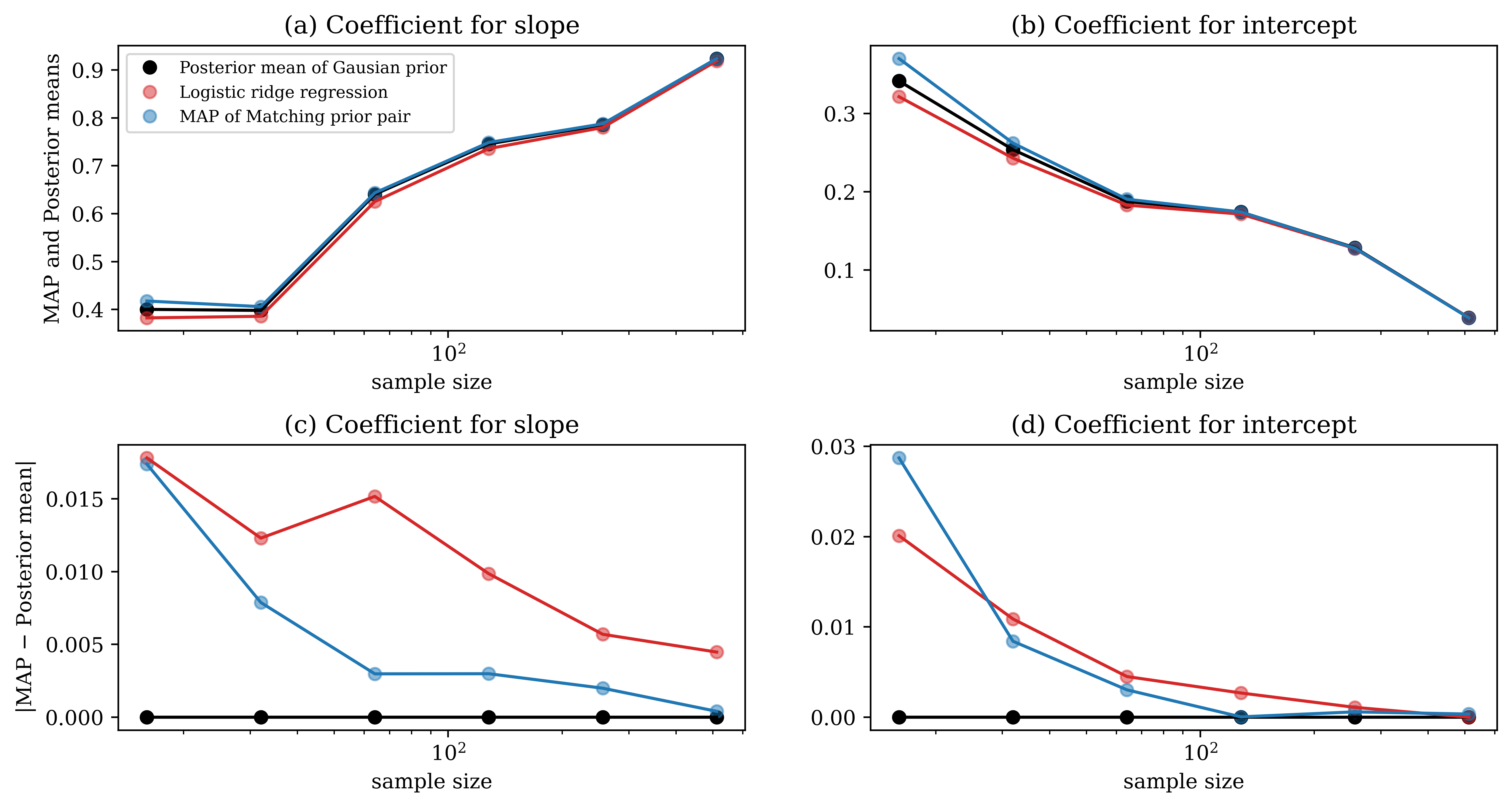
Figure 1: The posterior mean based on the Gaussian prior (colored in black), the logistic ridge regression (colored in red), and the MAP estimate based on the matching prior pair (colored in blue) under the correctly specified logistic regression model. (a)-(b) estimates themselves; (c)-(d) the differences with respect to the posterior mean based on the Gaussian prior. The horizontal axis adopts a logarithmic scale.

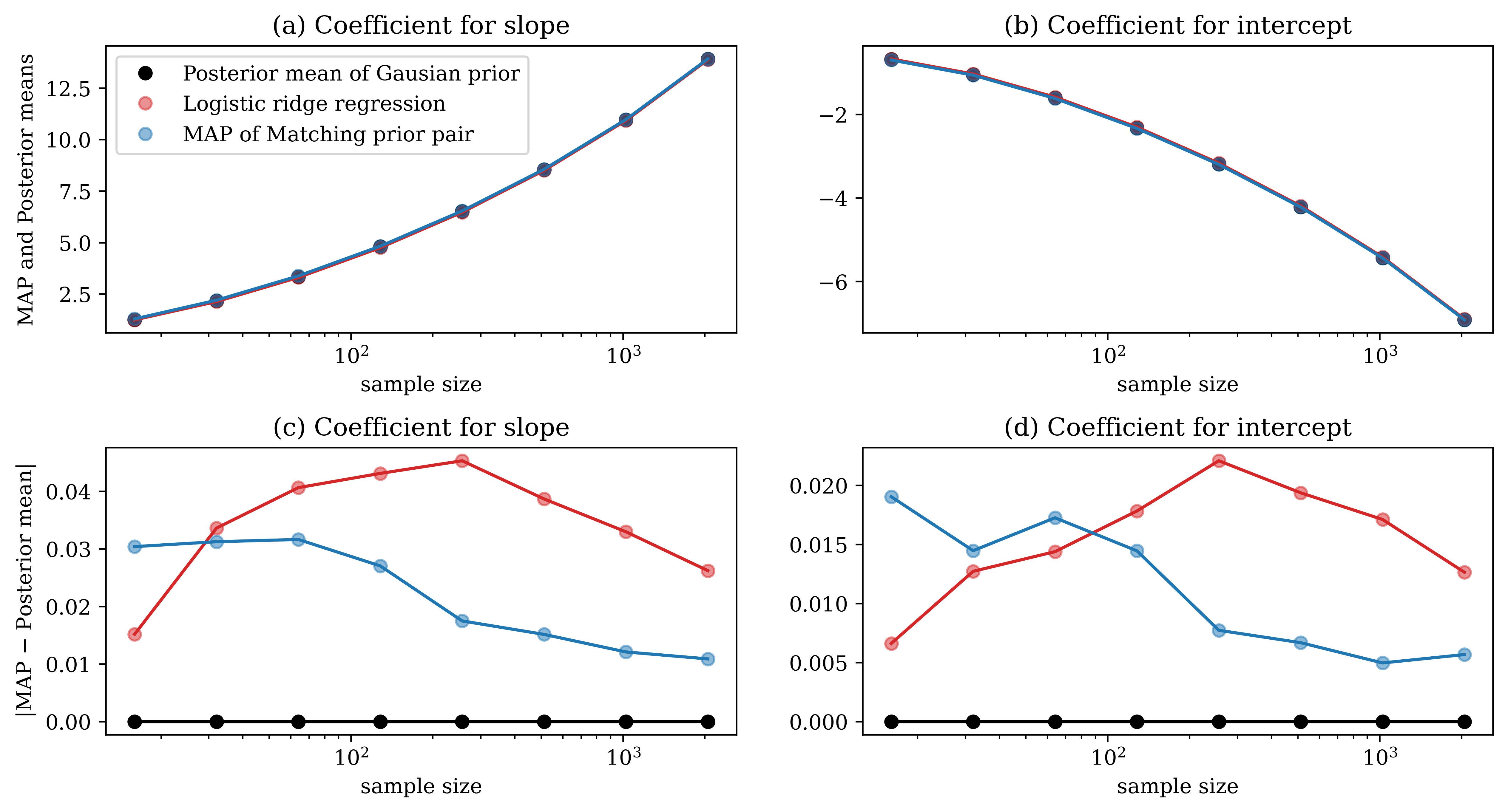
Figure 2: The posterior mean based on the Gaussian prior (colored in black), the logistic ridge regression (colored in red), and the MAP estimate based on the matching prior pair (colored in blue) under the misspecified logistic regression model. (a)-(b) estimates themselves; (c)-(d) the differences with respect to the posterior mean based on the Gaussian prior. The horizontal axis adopts a logarithmic scale.

Bayesian logistic regression model is a Bayesian version of the popular logistic regression model. By putting a Gaussian prior on regression coefficients, the working model becomes

$$Y(i)\mid X(i)\,,\,\beta \sim\mathrm{Bernoulli}(\sigma(X(i)\beta))\,\,(i=1,\ldots,n),$$

$$\beta \sim\mathrm{Normal}(0,I),$$

where $\sigma(x)=1/\{1+\exp(-x)\}$. This Bayesian model has been sometimes related to the logistic ridge regression:

$$\operatorname*{arg\,max}_{\beta}\left\{\sum_{i=1}^{n}l(y(i),x(i)\,;\,\beta)-\frac{\|\beta\|^{2}}{2}\right\}$$

with $l(y(i),x(i)\,;\,\beta):=y(i)\log\sigma(x(i)\beta)+(1-y(i))\log\{1-\sigma(x(i)\beta)\}$. Our theory tells a gap between the posterior mean based on the Gaussian prior $\pi_{\mathrm{PM}}(\beta)$ and the logistic ridge regression (the MAP estimate based on $\pi_{\mathrm{PM}}$). Also, the matching prior pair (5) gives another prior $\pi_{\mathrm{MAP}}$ yielding the MAP estimate asymptotically equal to the posterior mean of $\pi_{\mathrm{PM}}$

$$\pi_{\mathrm{MAP}}(\beta)\propto\left|\sum_{i=1}^{n}(X(i))^{\top}X(i)\left[\sigma(X(i)\beta)\{1-\sigma(X(i)\beta)\}\right]\right|^{-1/2}\pi_{\mathrm{PM}}(\beta),$$

inducing the following optimization:

$$\operatorname*{arg\,max}_{\beta}\left\{\sum_{i=1}^{n}l(y(i),x(i)\,;\,\beta)-\frac{1}{2}\|\beta\|^{2}-\frac{1}{2}\log\left|\sum_{i=1}^{n}(X(i))^{\top}X(i)\left[\sigma(X(i)\beta)\{1-\sigma(X(i)\beta)\}\right]\right|\right\}.$$

First, we check the behaviour of the matching prior pair by using the following two synthetic data:

$$X^{(1)}(i) =i/n,$$

$$Y^{(1)}(i)\mid X^{(1)}(i) \sim\sigma(X^{(1)}(i)+0.),$$

and

$$(Y^{(2)}(i),X^{(2)}(i))=\begin{cases}(1,i/n)\,\,\text{if}\,\,i>n/2,\\ (0,i/n)\,\,\text{if otherwise}.\end{cases}$$

The logistic regression model with 2-dimensional parameters (slope and intercept) applied to the former data $\{(Y^{(1)}(i),X^{(1)}(i))\,:\,i=1,\ldots,n\}$ is correctly-specified, while the model applied to the latter data $\{(Y^{(2)}(i),X^{(2)}(i))\,:\,i=1,\ldots,n\}$ is misspecified. The former data is random and so we take the mean of the performance using 50 repetitions. For the calculation of the posterior mean, we use the 10000 Markov chain Monte Carlo samples after the 10000 burnin samples by conducting the Pólya-Gamma augmentation (Polson and Scott, 2016). We vary the sample size in $\{2^{t}:t=4,5,6,7,8,9\}$ for the former case and in $\{2^{t}:t=4,5,6,7,8,9,10,11\}$ for the latter case, respectively.

Figures 1 and 2 display the results. From Figure 1, we see that under the correctly-specified model, the gap between the logistic ridge regression and the posterior mean based on the Gaussian prior is larger than the gap between the MAP estimate based on the matching prior pair and the posterior mean based on the Gaussian prior. Both gaps become smaller as the sample size gets larger. Figure 2 showcases the performance under the misspecified model. The performance with small sample sizes seems random but with moderate or large sample sizes, the MAP estimate based on the matching prior pair gets closer to the posterior mean based on the Gaussian prior. In both cases, there exists a gap between the logistic ridge regression and the posterior mean based on the Gaussian prior, and the matching prior pair reduces this gap.

Next, we check the performance of the matching prior pair by the banknote authentication data from UCI Machine Learning Repository (Dua and Graff, 2017). The banknote authentication data set classifies genuine and forged banknote-like specimens based on four image features (Variance, Skewness, Curtosis, and Entropy). The number of unknown parameters in this case is 4. We check the performance for sample sizes of $\{2^{t}:t=4,5,6,7,8,9,10\}$. For each sample size, we take indices randomly taken 50 times and then take the average of the performance.

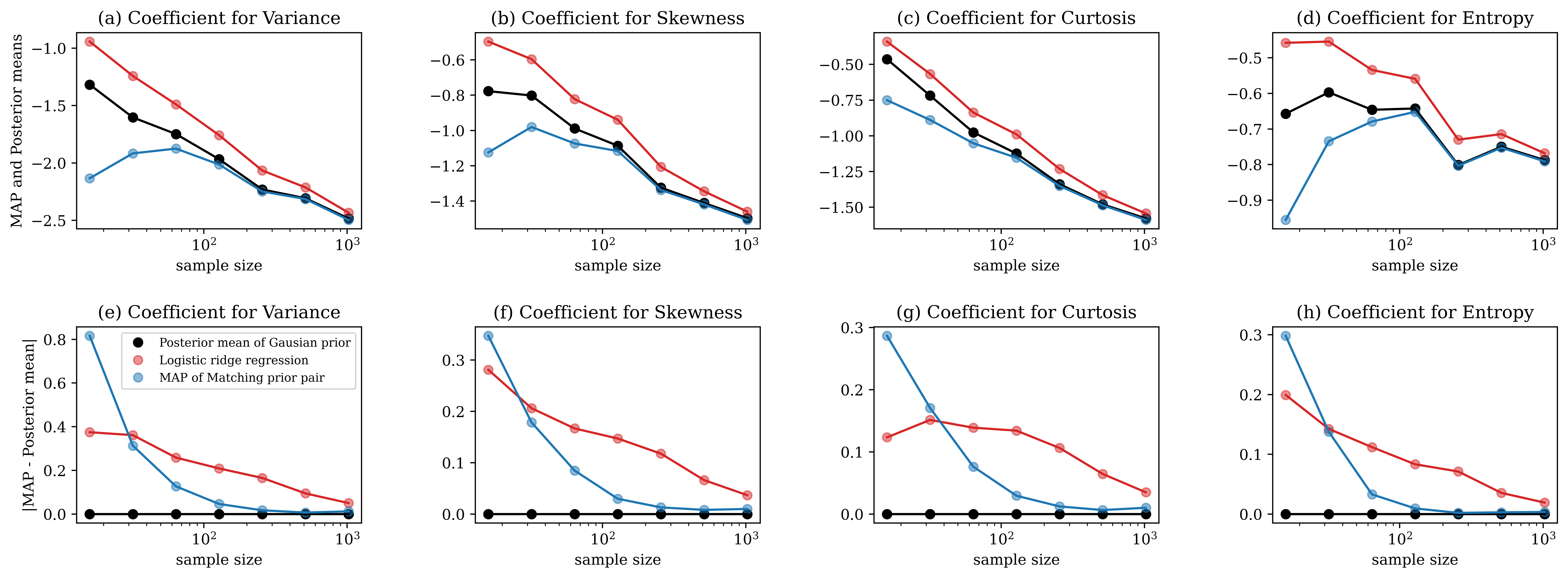
Figure 3: The Posterior mean based on the Gaussian prior (colored in black), the logistic ridge regression (colored in red), and the MAP estimate based on the matching prior pair (colored in blue) for the banknote authentification data. (a)-(b) estimates themselves; (c)-(d) the differences with respect to the posterior mean based on the Gaussian prior. The horizontal axis adopts a logarithmic scale.

Figure 3 displays the result. For all four variables, the matching prior pair reduces the gap with respect to the posterior mean based on the Gaussian prior except for small sample sizes. Although there seem some biases for the coefficients of Skewness and Curtosis, we note that there exist deviations from the theoretical values of the posterior means due to the randomness in MCMC. Overall, the calibration based on the matching prior pair works well for the logistic regression model.

3.2 The Poisson shrinkage model

Poisson sequence model is a canonical model for count-data analysis. Recently, incorporating the high-dimensional structure with Poisson sequence model has been well investigated (Komaki, 2004; Datta and Dunson, 2016; Yano et al., 2021; Hamura et al., 2022). Our focus here is to investigate the calibration based on the matching prior pair in high-dimension and under an improper prior. We work with the following model and the improper shrinkage prior proposed by Komaki (2006):

$$Y(i)=(Y_{1}(i),\ldots,Y_{d}(i))\mid\lambda=(\lambda_{1},\ldots,\lambda_{d}) \sim\otimes_{i=1}^{d}\mathrm{Poisson}(\lambda_{i})\,\,(i=1,\ldots,n),$$

$$\pi(\lambda) =\frac{\lambda_{1}^{\beta_{1}-1}\cdots\lambda_{d}^{\beta_{d}-1}}{(\lambda_{1}+\cdots+\lambda_{d})^{\alpha}},$$

where $\alpha>0$ and $\beta=(\beta_{1},\ldots,\beta_{d})$. The number of dimension $d$ is $100$ for synthetic data analysis and is $99$ for real data analysis, respectively. In the subsequent experiments, we set $\beta=(3,\ldots,3)$ and $\alpha=\sum_{j=1}^{d}\beta_{j}-1$.

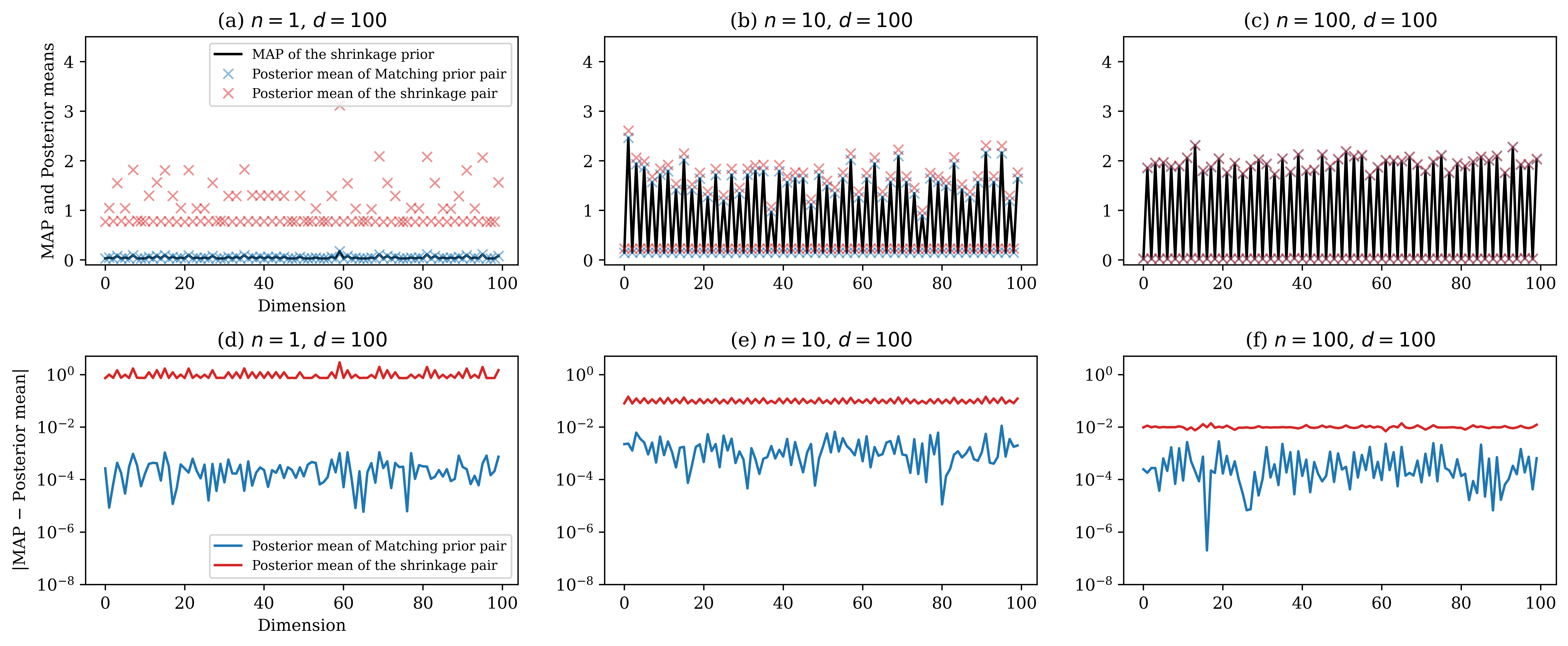
Figure 4: The MAP estimate based on the shrinkage prior (colored in black), the posterior mean based on the shrinkage prior (colored in red), and the posterior mean based on the matching prior pair (colored in blue) under the synthetic Poisson sequence model. (a)-(c) estimates themselves; (d)-(f) the differences with respect to the MAP estimate based on the shrinkage prior.

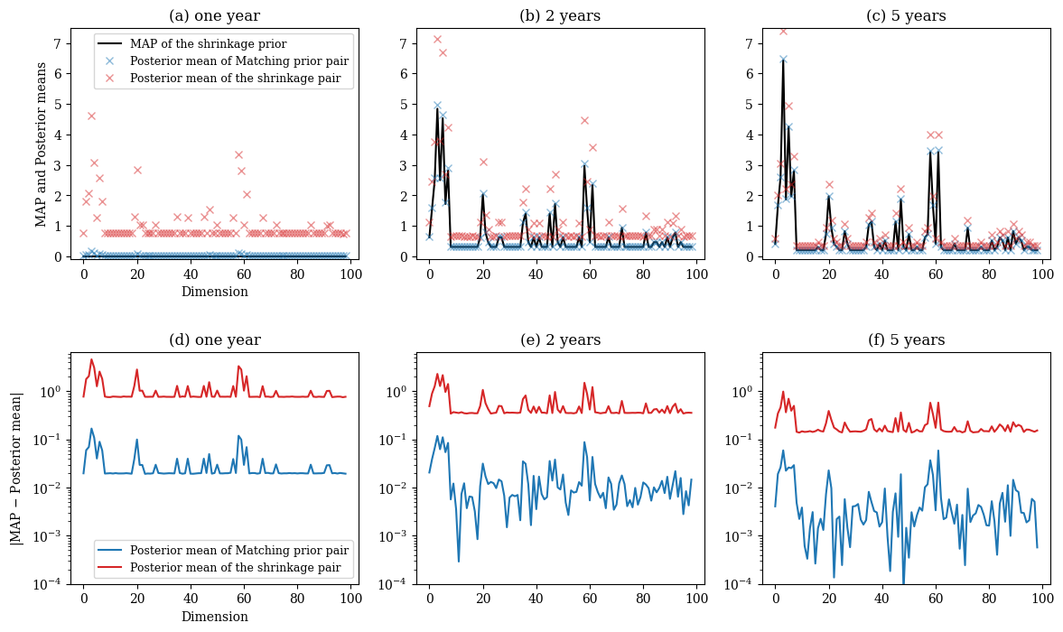
Figure 5: The MAP estimate based on the shrinkage prior (colored in black), the posterior mean based on the shrinkage prior (colored in red), and the posterior mean based on the matching prior pair (colored in blue) for pickpockets in Chuo ward, Tokyo, Japan. (a) estimates using only data for the entire year of 2012; (b) estimates using data from the two-year period of 2012-2013; (c) estimates using data from the five-year period of 2012-2016;(d)-(f) the differences with respect to the MAP estimate based on the shrinkage prior.

We begin with displaying the numerical experiment using the following synthetic data:

$$Y(i)=(Y_{1}(i),\ldots,Y_{d}(i))\mid\lambda=(\lambda_{1},\ldots,\lambda_{d}) \sim\otimes_{i=1}^{d}\mathrm{Poisson}(\lambda_{i})\,\,(i=1,\ldots,n),$$

$$\lambda_{j} =\begin{cases}0.001&\text{if}\,\,j\,\,\text{is odd},\\ 2&\text{if otherwise}.\end{cases}$$

In this experiment, we display the result for one realization because the result is not so much dependent on realization. For the calculation of the posterior mean, we use 10000 MCMC samples.

Figure 4 showcases the MAP estimate based on the shrinkage prior (colored in black), the posterior mean based on the shrinkage prior (colored in red), and the posterior mean based on the matching prior pair (colored in blue). From (d)-(f) of Figure 4, we see that the posterior mean based on the matching prior pair of the shrinkage prior can get closer to the MAP estimate based on the shrinkage prior than that based on the shrinkage prior. Surprisingly, even for high dimensional cases such as $(n,d)=(1,100)$ and $(n,d)=(10,100)$, the matching prior pair works well. One of potential reasons for this success in high dimension is that a Laplace approximation of the posterior distribution might still work in certain high-dimensional set-ups (e.g., Panov and Spokoiny, 2015; Yano and Kato, 2020; Kasprzaki et al., 2023).

We proceed to an application to Japanese pickpocket data from an official database (Department, 2023). This data reports the total numbers of pickpockets in each year in Tokyo Prefecture, and are classified by town and also by the type of crimes. We use pickpocket data from 2012 to 2016 at 99 towns in Chuo ward. We work with the Poisson sequence model ($d=99$, $n\leq 5$; $n$ is the number of years we use in the analysis) and report how the matching prior pair calibrates the shrinkage prior so as to get the posterior mean closer to the MAP estimate based on the shrinkage prior. For the calculation of the posterior mean, we use 10000 MCMC samples.

Figure 5 showcases the MAP estimate based on the shrinkage prior $\pi$ (colored in black), the posterior mean based on the shrinkage prior $\pi$ (colored in red), and the posterior mean based on the matching prior pair of $\pi$ (colored in blue) for pickpockets in Chuo ward, Tokyo, Japan. Figure 5 shows that for pickpocket data, the MAP estimate and the posterior mean based on the same shrinkage prior are different although the difference gets smaller as the sample size becomes larger, and the matching prior pair successfully yields the posterior mean closer to the MAP estimate based on the improper shrinkage prior.

4 Proofs

This section provides the proof of the main results.

Proof of Theorem 2.1.

The proof employs the following asymptotic expansions for a posterior mean and a MAP estimate.

Lemma 4.1.

The posterior mean of $\theta$ based on a prior $\pi_{\rm PM}(\theta)$ is expanded as

$$\hat{\theta}_{\rm PM}^{a}=\hat{\theta}_{\rm MLE}^{a} +\frac{{g}^{ab}(\hat{\theta}_{\rm MLE})}{n}\left(\partial_{b}\log\frac{\pi_{\rm PM}}{{\pi}_{\rm J}}(\hat{\theta}_{\rm MLE})+\frac{T_{b}(\hat{\theta}_{\rm MLE})}{2}\right)$$

$$+\frac{{g}^{bc}(\hat{\theta}_{\rm MLE})}{2n}\left(-\raise 1.5pt\hbox{$\displaystyle\mathop{\Gamma}^{\rm m}$}_{bc}^{\,~{}a}(\hat{\theta}_{\rm MLE})\right)+\mathrm{o}_{p}(n^{-1})\quad(a=1,\ldots,d).$$ (11)

Lemma 4.2.

The MAP estimate of $\theta$ based on a prior $\pi_{\rm MAP}(\theta)$ is expanded as

$$\hat{\theta}_{\rm MAP}^{a}=\hat{\theta}_{\rm MLE}^{a}+\frac{{g}^{ab}(\hat{\theta}_{\rm MLE})}{n}\partial_{b}\log{\pi_{\rm MAP}}(\hat{\theta}_{\rm MLE})+\mathrm{o}_{p}(n^{-1})\quad(a=1,\ldots,d).$$ (12)

The proofs of these lemmas are given right after the main proof.

These lemmas give the following condition under which the posterior mean $\hat{\theta}_{{\rm PM}}$ (4.3) and the MAP estimate $\hat{\theta}_{\rm MAP}$ (12) coincide except for $o_{p}(n^{-1})$ terms: for $a=1,\ldots,d$,

$$\frac{{g}^{ab}(\hat{\theta}_{\rm MLE})}{n}\left(\partial_{b}\log\frac{\pi_{\rm PM}}{{\pi}_{\rm J}}(\hat{\theta}_{\rm MLE})+\frac{T_{b}(\hat{\theta}_{\rm MLE})}{2}\right)+\frac{{g}^{bc}(\hat{\theta}_{\rm MLE})}{2n}\left(-\raise 1.5pt\hbox{$\displaystyle\mathop{\Gamma}^{\rm m}$}_{bc}^{\,~{}a}(\hat{\theta}_{\rm MLE})\right)$$

$$=\frac{{g}^{ab}(\hat{\theta}_{\rm MLE})}{n}\partial_{b}\log{\pi_{\rm MAP}}(\hat{\theta}_{\rm MLE})+\mathrm{o}_{p}(n^{-1}).$$

This is rewritten as

$${{g}^{ab}(\hat{\theta}_{\rm MLE})}\partial_{b}\log\frac{\pi_{\rm PM}}{{\pi}_{\rm MAP}}(\hat{\theta}_{\rm MLE})$$

$$={g}^{ab}(\hat{\theta}_{\rm MLE})\left(\partial_{b}\log{\pi_{\rm J}}(\hat{\theta}_{\rm MLE})-\frac{T_{b}(\hat{\theta}_{\rm MLE})}{2}\right)+\frac{{g}^{bc}(\hat{\theta}_{\rm MLE})}{2}\raise 1.5pt\hbox{$\displaystyle\mathop{\Gamma}^{\rm m}$}_{bc}^{\,~{}a}(\hat{\theta}_{\rm MLE})+\mathrm{o}_{p}(n^{-1})$$

$$={g}^{ab}(\hat{\theta}_{\rm MLE})\left[\partial_{b}\log{\pi_{\rm J}}(\hat{\theta}_{\rm MLE})-\frac{1}{2}\left\{\raise 1.5pt\hbox{$\displaystyle\mathop{\Gamma}^{\rm m}$}_{cdb}^{\,}(\hat{\theta}_{\rm MLE})-\raise 1.5pt\hbox{$\displaystyle\mathop{\Gamma}^{\rm e}$}_{cdb}^{\,}(\hat{\theta}_{\rm MLE})\right\}g^{cd}(\hat{\theta}_{\rm MLE})\right]$$ (13)

$$\quad+\frac{{g}^{bc}(\hat{\theta}_{\rm MLE})}{2}\raise 1.5pt\hbox{$\displaystyle\mathop{\Gamma}^{\rm m}$}_{bc}^{\,~{}a}(\hat{\theta}_{\rm MLE})+\mathrm{o}_{p}(n^{-1})$$

$$={g}^{ab}(\hat{\theta}_{\rm MLE})\partial_{b}\log{\pi_{\rm J}}(\hat{\theta}_{\rm MLE})+\frac{{g}^{bc}(\hat{\theta}_{\rm MLE})}{2}\raise 1.5pt\hbox{$\displaystyle\mathop{\Gamma}^{\rm e}$}_{bc}^{\,~{}a}(\hat{\theta}_{\rm MLE})+\mathrm{o}_{p}(n^{-1}),$$ (14)

where the second identity follows since $T_{abc}=\raise 1.5pt\hbox{$\displaystyle\mathop{\Gamma}^{\rm m}$}_{abc}^{\,}-\raise 1.5pt\hbox{$\displaystyle\mathop{\Gamma}^{\rm e}$}_{abc}^{\,}$. This completes the proof. ∎

Proof of Lemma 4.1.

In the proof, we consider an approximation of the posterior expectation of arbitrary third-times differentiable function $f:\Theta\to\mathbb{R}$. Setting $f(\theta)=\theta^{a}$ ($a=1,\ldots,d$) gives the approximation of the posterior mean of $\theta$. The following proof of Lemma 4.1 proceeds closely following the proof of Theorem III.1 in Okudo and Komaki (2021). The first step is to employ the Laplace approximation of integrals to get an approximation of the posterior expectation. The second step is to arrange terms in information-geometrical notations.

Step 1: Laplace approximation. Observe that the posterior expectation of a third-times differentiable function $f(\theta)$ based on a prior $\pi(\theta)$ is written as

$$f_{\pi}(y^{n})=\frac{\int f(\theta)p(y^{n}\,;\,\theta)\pi(\theta)d\theta}{\int p(y^{n}\,;\,\theta)\pi(\theta)d\theta}=\frac{\int f(\theta)\exp(n\bar{L}(\theta))\pi(\theta)d\theta}{\int\exp(n\bar{L}(\theta))\pi(\theta)d\theta},$$

where $\bar{L}(\theta)=(1/n)\sum_{t=1}^{n}\log p(y(t)\,;\,\theta)$. We approximate this using the Laplace method (e.g., Theorem 4.6.1 of Kass and Vos (1997) and Tierney and Kadane (1986)). Consider an expansion of $\pi(\theta)\exp(n\bar{L}(\theta))$ around $\theta=\hat{\theta}_{\rm MLE}$. In the following, for any function $g(\theta)$, we abbreviate the value $g(\hat{\theta}_{\rm MLE})$ to $\hat{g}$; e.g., $\hat{\pi}:=\pi(\hat{\theta}_{\rm MLE})$. By rescaling $\theta$ as $\theta=\hat{\theta}_{\rm MLE}+\phi/\sqrt{n}$, we get

$$\pi(\theta)\exp(n\bar{L}(\theta))$$

$$=\left(\hat{\pi}+\frac{(\partial_{a}\hat{\pi})\phi^{a}}{\sqrt{n}}+\frac{(\partial_{ab}\hat{\pi})\phi^{a}\phi^{b}}{2n}+\frac{(\partial_{abc}\hat{\pi})\phi^{a}\phi^{b}\phi^{c}}{6n\sqrt{n}}+\mathrm{O}_{p}(n^{-2})\right)$$

$$~{}~{}~{}\times\exp\left(n\hat{L}+\frac{(\partial_{ab}\hat{L})\phi^{a}\phi^{b}}{2}+\frac{(\partial_{abc}\hat{L})\phi^{a}\phi^{b}\phi^{c}}{6\sqrt{n}}+\frac{(\partial_{abcd}\hat{L})\phi^{a}\phi^{b}\phi^{c}\phi^{d}}{24{n}}+\frac{(\partial_{abcde}\hat{L})\phi^{a}\phi^{b}\phi^{c}\phi^{d}\phi^{e}}{120n\sqrt{n}}\right.$$

$$~{}~{}~{}~{}~{}~{}~{}~{}~{}~{}~{}~{}~{}~{}~{}\left.+\mathrm{O}_{p}(n^{-2})\right)$$

$$=\hat{\pi}e^{n\hat{L}}e^{(\partial_{ab}\hat{L})\phi^{a}\phi^{b}/2}\left(1+\frac{(\partial_{a}\hat{\pi})\phi^{a}}{\hat{\pi}\sqrt{n}}+\frac{(\partial_{ab}\hat{\pi})\phi^{a}\phi^{b}}{2\hat{\pi}n}+\frac{(\partial_{abc}\hat{\pi})\phi^{a}\phi^{b}\phi^{c}}{6\hat{\pi}n\sqrt{n}}+\mathrm{O}_{p}(n^{-2})\right)$$

$$~{}~{}~{}\times\left(1+\frac{(\partial_{abc}\hat{L})\phi^{a}\phi^{b}\phi^{c}}{6\sqrt{n}}+\frac{(\partial_{abcd}\hat{L})\phi^{a}\phi^{b}\phi^{c}\phi^{d}}{24{n}}+\frac{(\partial_{abc}\hat{L})(\partial_{a^{\prime}b^{\prime}c^{\prime}}\hat{L})\phi^{a}\phi^{b}\phi^{c}\phi^{a^{\prime}}\phi^{b^{\prime}}\phi^{c^{\prime}}}{72{n}}+\mathrm{O}_{p}(n^{-3/2})\right)$$

$$=\hat{\pi}e^{n\hat{L}}e^{-\hat{J}_{ab}\phi^{a}\phi^{b}/2}\left(1+\frac{(\partial_{a}\hat{\pi})\phi^{a}}{\hat{\pi}\sqrt{n}}{+\frac{(\partial_{abc}\hat{L})\phi^{a}\phi^{b}\phi^{c}}{6\sqrt{n}}}+\frac{(\partial_{ab}\hat{\pi})\phi^{a}\phi^{b}}{2\hat{\pi}n}+\frac{(\partial_{a}\hat{\pi})(\partial_{bcd}\hat{L})\phi^{a}\phi^{b}\phi^{c}\phi^{d}}{6\hat{\pi}n}\right.$$

$$~{}~{}\left.+\frac{(\partial_{abc}\hat{\pi})\phi^{a}\phi^{b}\phi^{c}}{6\hat{\pi}n\sqrt{n}}+\frac{(\partial_{ab}\hat{\pi})(\partial_{cde}\hat{L})\phi^{a}\phi^{b}\phi^{c}\phi^{d}\phi^{e}}{12\hat{\pi}n\sqrt{n}}+\frac{(\partial_{a}\hat{\pi})(\partial_{bcde}\hat{L})\phi^{a}\phi^{b}\phi^{c}\phi^{d}\phi^{e}}{24\hat{\pi}n\sqrt{n}}\right.$$

$$~{}~{}\left.+\frac{(\partial_{a}\hat{\pi})(\partial_{bcd}\hat{L})(\partial_{efg}\hat{L})\phi^{a}\phi^{b}\phi^{c}\phi^{d}\phi^{e}\phi^{f}\phi^{g}}{72\hat{\pi}n\sqrt{n}}{+\frac{C_{1}}{n}}+\mathrm{O}_{p}(n^{-2})\right),$$ (15)

where the second equation follows from $\exp(x)=1+x+O(x^{2})$, and in the third equation, we denote $-\partial_{ab}\hat{L}$ by $\hat{J}_{ab}$ and denote terms not depending on $\pi$ and $n$ by $C_{1}$, respectively.

Next, we integrate both sides of (15) with respect to $\theta$. Let $(\hat{J}^{ab})$ be the inverse matrix of $(\hat{J}_{ab})$. By changing the variables from $\theta$ to $\phi$, and by using the formula of moments of multivariate Gaussian distributions, we obtain

$$\int\pi(\theta)\exp(n\bar{L}(\theta))d\theta$$

$$=C_{2}\hat{\pi}\left(1+\frac{(\partial_{ab}\hat{\pi})}{2\hat{\pi}n}\int\phi^{a}\phi^{b}e^{-\hat{J}_{cd}\phi^{c}\phi^{d}/2}d\phi+\frac{(\partial_{a}\hat{\pi})(\partial_{bcd}\hat{L})}{6\hat{\pi}n}\int\phi^{a}\phi^{b}\phi^{c}\phi^{d}e^{-\hat{J}_{ef}\phi^{e}\phi^{f}/2}d\phi\right.$$

$$\left.\quad\quad\quad\quad+\frac{C_{1}}{n}+\mathrm{O}_{p}(n^{-2})\right)$$

$$=C_{2}\hat{\pi}\left(1+\frac{(\partial_{ab}\hat{\pi})\hat{J}^{ab}}{2\hat{\pi}n}+\frac{(\partial_{a}\hat{\pi})(\partial_{bcd}\hat{L})(\hat{J}^{ab}\hat{J}^{cd}+\hat{J}^{ac}\hat{J}^{bd}+\hat{J}^{ad}\hat{J}^{bc})}{6\hat{\pi}n}+{\frac{C_{1}}{n}}+\mathrm{O}_{p}(n^{-2})\right)$$

$$=C_{2}\hat{\pi}\left(1+\frac{(\partial_{ab}\hat{\pi})\hat{J}^{ab}}{2\hat{\pi}n}+\frac{(\partial_{a}\hat{\pi})(\partial_{bcd}\hat{L})\hat{J}^{ab}\hat{J}^{cd}}{2\hat{\pi}n}+{\frac{C_{1}}{n}}+\mathrm{O}_{p}(n^{-2})\right),$$

where $C_{2}$ is a constant not depending on $\pi$ and $n$. Replacing $\pi(\theta)$ by $f(\theta)\pi(\theta)$ for an arbitrary third-times differentiable function $f:\mathbb{R}^{d}\to\mathbb{R}$, we have

$$\int f(\theta)\pi(\theta)\exp(nL(\theta))d\theta$$

$$=C_{2}\hat{f}\hat{\pi}\left(1+\frac{\{\partial_{ab}(\hat{f}\hat{\pi})\}\hat{J}^{ab}}{2\hat{f}\hat{\pi}n}+\frac{\{\partial_{a}(\hat{f}\hat{\pi})\}(\partial_{bcd}\hat{L})\hat{J}^{ab}\hat{J}^{cd}}{2\hat{f}\hat{\pi}n}+{\frac{C_{1}}{n}}+\mathrm{O}_{p}(n^{-2})\right).$$

Therefore, the posterior expectation of $f(\theta)$ is expanded as

$$f_{\pi} =\frac{\int f(\theta)\exp(nL(\theta))\pi(\theta)d\theta}{\int\exp(nL(\theta))\pi(\theta)d\theta}$$

$$=\left.C_{2}\hat{f}\hat{\pi}\left(1+\frac{\partial_{ab}(\hat{f}\hat{\pi})\hat{J}^{ab}}{2\hat{f}\hat{\pi}n}+\frac{\{\partial_{a}(\hat{f}\hat{\pi})\}(\partial_{bcd}\hat{L})\hat{J}^{ab}\hat{J}^{cd}}{2\hat{f}\hat{\pi}n}+{\frac{C_{1}}{n}}+\mathrm{O}_{p}(n^{-2})\right)\right.$$

$$~{}~{}~{}\left.\middle/C_{2}\hat{\pi}\left(1+\frac{(\partial_{ab}\hat{\pi})\hat{J}^{ab}}{2\hat{\pi}n}+\frac{(\partial_{a}\hat{\pi})(\partial_{bcd}\hat{L})\hat{J}^{ab}\hat{J}^{cd}}{2\hat{\pi}n}+{\frac{C_{1}}{n}}+\mathrm{O}_{p}(n^{-2})\right)\right.$$

$$=\hat{f}\left(1+\frac{\hat{J}^{ab}}{2n}\left(\frac{\partial_{ab}(\hat{f}\hat{\pi})}{\hat{\theta}_{i}\hat{\pi}}-\frac{\partial_{ab}\hat{\pi}}{\hat{\pi}}\right)+\frac{\hat{J}^{ab}\hat{J}^{cd}\partial_{bcd}\hat{L}}{2n}\left(\frac{\partial_{a}(\hat{f}\hat{\pi})}{\hat{\theta}\hat{\pi}}-\frac{\partial_{a}\hat{\pi}}{\hat{\pi}}\right)+\mathrm{O}_{p}(n^{-2})\right)$$

$$=\hat{f}+\frac{\hat{J}^{ab}}{2n}\left(\partial_{ab}\hat{f}+\frac{2(\partial_{a}\hat{f})(\partial_{b}\hat{\pi})}{\hat{\pi}}\right)+\frac{\hat{J}^{ab}\hat{J}^{cd}\partial_{bcd}\hat{L}}{2n}\partial_{a}\hat{f}+\mathrm{O}_{p}(n^{-2}).$$ (16)

This completes Step 1.

Step 2: Rearrangement using the information-geometric notations. The law of large numbers yields $\hat{J}_{ab}=\hat{g}_{ab}+o_{p}(1)$ and $\partial_{bcd}\hat{L}=\mathrm{E}_{\theta}[\partial_{bcd}\hat{L}]+o_{p}(1)$. The Bartlett identity gives

$$\mathrm{E}_{\theta}[\partial_{bcd}L]=-\partial_{b}g_{cd}(\theta)-\raise 1.5pt\hbox{$\displaystyle\mathop{\Gamma}^{\rm e}$}_{cdb}^{\,}(\theta)=-\partial_{b}g_{cd}(\theta)-\raise 1.5pt\hbox{$\displaystyle\mathop{\Gamma}^{\rm m}$}_{cdb}^{\,}(\theta)+T_{bcd}(\theta).$$

Together with the definition of 0-parallel prior $g^{cd}\partial_{b}g_{cd}=\partial_{b}\log(|g|)=2\partial_{b}\log\pi_{\rm J}$, these give the following representation of the approximated posterior expectation of $f$:

$$f_{\pi} =\hat{f}+\frac{\hat{g}^{ab}}{2n}\left(\partial_{ab}\hat{f}+2\partial_{a}\hat{f}\partial_{b}\log\hat{\pi}\right)$$

$$\quad\quad+\frac{\hat{g}^{ab}}{2n}\left(-2\partial_{b}\log\hat{\pi}_{J}-\hat{g}^{cd}\raise 1.5pt\hbox{$\displaystyle\mathop{\Gamma}^{\rm m}$}_{cdb}^{\,}(\hat{\omega}_{\rm MLE})+T_{b}(\hat{\omega}_{\rm MLE})\right)\partial_{a}\hat{f}+\mathrm{o}_{p}(n^{-1})$$

$$=\hat{f}+\frac{\hat{g}^{ab}}{2n}\left(\partial_{ab}\hat{f}-\raise 1.5pt\hbox{$\displaystyle\mathop{\Gamma}^{\rm m}$}_{ab}^{\,~{}c}(\hat{\omega}_{\rm MLE})\partial_{c}\hat{f}\right)+\frac{\hat{g}^{ab}}{n}\left(\partial_{b}\log\frac{\hat{\pi}}{\hat{\pi}_{J}}+\frac{T_{b}(\hat{\omega}_{\rm MLE})}{2}\right)\partial_{a}\hat{f}+\mathrm{o}_{p}(n^{-1}).$$

Thus, replacing $f$ by $\theta^{a}$, we have

$$\hat{\theta}^{a}_{\rm PM} =\hat{\theta}^{a}+\frac{\hat{g}^{bc}}{2n}\left(-\raise 1.5pt\hbox{$\displaystyle\mathop{\Gamma}^{\rm m}$}_{bc}^{\,~{}a}(\hat{\theta}_{\rm MLE})\right)+\frac{\hat{g}^{ab}}{n}\left(\partial_{b}\log\frac{\hat{\pi}}{\hat{\pi}_{J}}+\frac{T_{b}(\hat{\theta}_{\rm MLE})}{2}\right)+\mathrm{o}_{p}(n^{-1}).$$

∎

Proof of Lemma 4.2.

Observe the definition of the MAP estimate $\hat{\theta}_{\rm MAP}$:

$$n\partial_{a}\bar{L}(\hat{\theta}_{\rm MAP})+\partial_{a}\log\pi(\hat{\theta}_{\rm MAP})=0\,\,(a=1,\ldots,d),$$

where $\bar{L}(\theta)=(1/n)\sum_{t=1}^{n}\log p(y(t)\,;\,\theta)$. Letting $\delta=\hat{\theta}_{\rm MAP}-\hat{\theta}_{\rm MLE}$, the Taylor expansion around $\hat{\theta}_{\rm MLE}$ yields, for $a=1,\ldots,d$,

$$0 =\partial_{a}\bar{L}(\hat{\theta}_{\rm MAP})+\frac{1}{n}\partial_{a}\log\pi(\hat{\theta}_{\rm MAP})$$

$$=\partial_{a}\bar{L}(\hat{\theta}_{\rm MLE})+\delta^{b}\partial_{ab}\bar{L}(\hat{\theta}_{\rm MLE})+\frac{1}{n}\partial_{a}\log\pi(\hat{\theta}_{\rm MLE})+{\rm O}_{p}(\|\delta\|^{2}),$$

$$=\delta^{b}\partial_{ab}\bar{L}(\hat{\theta}_{\rm MLE})+\frac{1}{n}\partial_{a}\log\pi(\hat{\theta}_{\rm MLE})+{\rm O}_{p}(\|\delta\|^{2}),$$

where the last equation follows since $\partial_{a}\bar{L}(\hat{\theta}_{\rm MLE})=0$ for $a=1,\ldots,d$. Because the law of large numbers and the central limit theorem give

$$\partial_{ab}\bar{L}(\hat{\theta}_{\rm MLE})=-g_{ab}(\hat{\theta}_{\rm MLE})+{\rm o}_{p}(1)\quad\text{and}\quad\partial_{ab}\bar{L}(\hat{\theta}_{\rm MLE})+g_{ab}(\hat{\theta}_{\rm MLE})={\rm O}_{p}(1/\sqrt{n}),$$

we get

$$\delta^{b}g_{ab}(\hat{\theta}_{\rm MLE})+{\rm O}_{p}(\|\delta\|/\sqrt{n})=\frac{1}{n}\partial_{a}\log\pi(\hat{\theta}_{\rm MLE})+{\rm O}_{p}(\|\delta\|^{2}),$$

which yields

$$\delta^{b} =\frac{1}{n}g^{ab}(\hat{\theta}_{\rm MLE})\partial_{a}\log\pi(\hat{\theta}_{\rm MLE})+{\rm o}_{p}(n^{-1})\,\,(b=1,\ldots,d)$$

and completes the proof. ∎

Proof of Proposition 4.4.

This proposition is proved simply by changing Lemmas 4.1-4.2 to the following lemmas.

Lemma 4.3.

For $i=1,\ldots,d$, the posterior mean of $f_{i}(\theta)$ based on a prior $\pi(\theta)$ is expanded as

$$(f_{\pi})_{i}= f_{i}(\hat{\theta}_{\rm MLE})+\frac{{g}^{ab}(\hat{\theta}_{\rm MLE})}{n}\left(\partial_{b}\log\frac{\pi}{{\pi}_{J}}(\hat{\theta}_{\rm MLE})+\frac{T_{b}(\hat{\theta}_{\rm MLE})}{2}\right)\partial_{a}f_{i}(\hat{\theta}_{\rm MLE})$$

$$+\frac{{g}^{bc}(\hat{\theta}_{\rm MLE})}{2n}\left(\partial_{b}\partial_{c}f_{i}(\hat{\theta}_{\rm MLE})-\raise 1.5pt\hbox{$\displaystyle\mathop{\Gamma}^{\rm m}$}_{bc}^{\,~{}a}(\hat{\theta}_{\rm MLE})\partial_{a}f_{i}(\hat{\theta}_{\rm MLE})\right)+\mathrm{o}_{p}(n^{-1}).$$

Lemma 4.4.

For $i=1,\ldots,d$, a plugin of the MAP estimate $\hat{\theta}_{\rm MAP}$ of $\theta$ based on a prior $\pi(\theta)$ into a statistic $f_{i}(\theta)$ is expanded as

$$f_{i}(\hat{\theta}_{\rm MAP})=f_{i}(\hat{\theta}_{\rm MLE})+\frac{{g}^{ab}(\hat{\theta}_{\rm MLE})}{n}\partial_{b}\log{\pi}(\hat{\theta}_{\rm MLE})\partial_{a}f_{i}(\hat{\theta}_{\rm MLE})+\mathrm{o}_{p}(n^{-1}).$$

The proofs of these lemmas are straightforward and omitted.

∎

5 Acknowledgements

The authors thank Kaoru Irie for helpful comments to the early version of this work. The authors also thank Ryoya Kaneko for sharing his python codes of data preprocessing. This work is supported by JSPS KAKENHI (JP19K20222, JP20K23316, JP21H05205, JP21K12067, JP22H00510, JP23K11024), MEXT (JPJ010217), and “Strategic Research Projects” grant (2022-SRP-13) from ROIS (Research Organization of Information and Systems).

References

- Amari (1985) S. Amari. Differential-Geometrical Methods in Statistics. Springer-Verlag, New York, 1985.
- Burger and Lucka (2014) M. Burger and F. Lucka. Maximum a posteriori estimates in linear inverse problems with log-concave priors are proper Bayes estimators. Inverse Problems, 30, 2014.
- Datta and Dunson (2016) J. Datta and D. Dunson. Bayesian inference on quasi-sparse count data. Biometrika, 103:971–983, 2016.
- Department (2023) Tokyo Metropolitan Police Department. The number of crimes in tokyo prefecture by town and type, 2023. https://www.keishicho.metro.tokyo.lg.jp/about_mpd/jokyo_tokei/jokyo/.
- Dua and Graff (2017) D. Dua and C. Graff. UCI machine learning repository, 2017. http://archive.ics.uci.edu/ml.
- Ghosh and Liu (2011) M. Ghosh and R. Liu. Moment matching priors. Sankhyā : The Indian Journal of Statistics, 73:185–201, 2011.
- Gribonval (2011) R. Gribonval. Should penalized least squares regression be interpreted as Maximum A Posteriori estimation? IEEE Transaction on Signal Processing, 59:2405–2410, 2011.
- Gribonval and Machart (2013) R. Gribonval and P. Machart. Reconciling “priors” & ”priors” without prejudice? Proceedings of Advances in Neural Information Processing Systems 26 (NIPS 2013), 2013.
- Hamura et al. (2022) H. Hamura, K. Irie, and S. Sugasawa. On global-local shrinkage priors for count data. Bayesian Analysis, 17:545–564, 2022.
- Hartigan (1998) J. Hartigan. The maximum likelihood prior. The Annals of Statistics, 26:2083–2103, 1998.
- Hashimoto (2019) S. Hashimoto. Moment matching priors for non-regular models. Journal of Statistical Planning and Inference, 203:169–177, 2019.
- Kasprzaki et al. (2023) M. Kasprzaki, R. Giordano, and T. Broderick. How good is your Laplace approximation of the Bayesian posterior? finite-sample computable error bounds for a variety of useful divergences, 2023. arXiv:2209.14992.
- Kass and Vos (1997) R. E. Kass and P. W. Vos. Geometrical Foundations of Asymptotic Inference. Wiley, New York, 1997.
- Komaki (1996) F. Komaki. On asymptotic properties of predictive distributions. Biometrika, 83:299–313, 1996.
- Komaki (2004) F. Komaki. Simultaneous prediction of independent Poisson observables. Annals of Statistics, 32:1744–1769, 2004.
- Komaki (2006) F. Komaki. Shrinkage priors for Bayesian prediction. Annals of Statistics, 34:808–819, 2006.
- Lauritzen (1987) S. Lauritzen. Statistical manifolds, chapter 4. Institute of Mathematical Statistic, 1987.
- Liu et al. (2014) R. Liu, A. Chakrabarti, T. Samanta, J. Ghosh, and M. Ghosh. On divergence measures leading to Jeffreys and other reference priors. Bayesian Analysis, 9:331–370, 2014.
- Louchet and Moisan (2013) C. Louchet and L. Moisan. Posterior expectation of the total variation model: Properties and experiments. SIAM JOurnal of Imaging Science, 6:2640–2684, 2013.
- Matsuda (1976) M. Matsuda. Theory of exterior differential forms. Iwanami shoten, 1976. in Japanese.
- Okudo and Komaki (2021) M. Okudo and F. Komaki. Bayes extended estimators for curved exponential families. IEEE Transactions on Information Theory, 67:1088–1098, 2021.
- Pananos and Lizotte (2020) A. Pananos and D. Lizotte. Comparisons between Hamiltonian Monte Carlo and Maximum A Posteriori for a Bayesian model for Apixaban induction dose & dose personalization. Proceedings of Machine Learning Research, 126:1–20, 2020.
- Panov and Spokoiny (2015) M. Panov and V. Spokoiny. Finite sample Bernstein–von Mises theorem for semiparametric problems. Bayesian Analysis, 10:665–710, 2015.
- Polson and Scott (2016) N. Polson and J. Scott. Mixtures, envelopes and hierarchical duality. Journal of the Royal Statistical Society Series B: Statistical Methodology, 78(4):701–727, 2016.
- Takeuchi and Amari (2005) J. Takeuchi and S. Amari. -parallel prior and its properties. IEEE transactions on information theory, 51(3):1011–1023, 2005.
- Tanaka (2023) F. Tanaka. Geometric properties of noninformative priors based on the chi-square divergence. Frontiers in Applied Mathematics and Statistics, 9, 2023.
- Tierney and Kadane (1986) L. Tierney and J. B. Kadane. Accurate approximations for posterior moments and marginal densities. Journal of the American Statistical Association, 81:82–86, 1986.
- Yanagimoto and Miyata (2023) T. Yanagimoto and Y. Miyata. A pair of novel priors for improving and extending the conditional MLE. Journal of Statistical Planning and Inference, in press:106–117, 2023.
- Yano and Kato (2020) K. Yano and K. Kato. On frequentist coverage errors of Bayesian credible sets in moderately high dimensions. Bernoulli, 26:616–641, 2020.
- Yano et al. (2021) K. Yano, R. Kaneko, and F. Komaki. Minimax predictive density for sparse count data. Bernoulli, 27:1212–1238, 2021.
- Zwillinger (1997) D. Zwillinger. Handbook of Differential Equations. Academic Press, third edition edition, 1997.