Joint State Estimation and Noise Identification Based on Variational Optimization

Abstract

In this article, the state estimation problems with unknown process noise and measurement noise covariances for both linear and nonlinear systems are considered. By formulating the joint estimation of system state and noise parameters into an optimization problem, a novel adaptive Kalman filter method based on conjugate-computation variational inference, referred to as CVIAKF, is proposed to approximate the joint posterior probability density function of the latent variables (i.e., the noise covariance matrices and system state). Unlike the existing adaptive Kalman filter methods utilizing variational inference in natural-parameter space, CVIAKF performs optimization in expectation-parameter space, resulting in a faster and simpler solution, particularly for nonlinear state estimation. Meanwhile, CVIAKF divides optimization objectives into conjugate and non-conjugate parts of nonlinear dynamical models, whereas conjugate computations and stochastic mirror-descent are applied, respectively. Remarkably, the reparameterization trick is used to reduce the variance of stochastic gradients of the non-conjugate parts. The effectiveness of CVIAKF is validated through synthetic and real-world datasets of maneuvering target tracking.

I Introduction

Most state estimation methods are based on the assumptions that the dynamical models and the noise covariance matrices of the studied system are known a priori. However, in practice, obtaining accurate statistics of the noise can be difficult or even impossible. For example, in noncooperative target tracking [1], the noise covariance matrices are often time-varying and unknown, arising from unexpected maneuvers of noncooperative targets and measurement outliers. In such cases, standard Kalman filtering methods that rely on knowledge of noise statistic parameters may lose their accuracy or even lead to filter divergence. To solve this problem, one must resort to an adaptive Kalman filter [2], which performs state estimation and noise identification simultaneously.

There are two primary categories of adaptive Kalman filter methods, namely model adaptive methods and parameter adaptive methods. The model adaptive methods consist of the so-called multiple model estimators [3], which perform the joint state estimation and model selection by employing a series of candidate models characterizing different system modes. Optimal state estimation is intractable for multiple model systems due to the exponential growth of hypotheses. Therefore, some suboptimal approaches have been investigated to reduce the number of underlying hypotheses, including the well-known interactive multiple model estimator (IMM) [4, 5]. The model adaptive methods show promising performance in maneuvering target tracking, signal processing, fault detection, etc. However, the requirement of available complete model sets restricts their capability of tackling model uncertainties. The parameter adaptive methods consist of the so-called equivalent-noise methods [6], whereas the transition function of the dynamic system and the measurement function of the sensor are known, and the equivalent noise quantifies the modeling error, e.g., maneuvers. The noise statistics are nonstationary and unknown, which need to be identified along with the state estimation. The main idea of parameter adaptive methods is to infer the intractable joint posterior probability density function (PDF) of system state and noise parameter. Closed-form analytical solutions may not exist for optimal Bayesian inference. In such situations, one needs to resort to approximation schemes. There are mainly two categories of methods, including sampling-based stochastic approximation [7] and optimizing-based deterministic approximation, which trade off speed, accuracy, simplicity, and generality. The sampling-based sequential Monte Carlo (SMC) [7] methods approximate the intractable joint PDFs via particle propagation [8]. However, their applicability is restricted to small-scale state estimation problems due to the significant computational burden they impose. The optimizing-based variational Bayes (VB) [9] reduces posterior inference into optimization, yielding an approximate analytical solution. Due to the efficient computation for high-dimensional estimation problems, VB-based methods have received ubiquitous interest in adaptive filtering applications.

Considering that the covariance matrix of the measurement noise is unknown, Särkkä and Nummenmaa [10] presented the first VB-based adaptive Kalman filtering, whereas the Gaussian Inverse-Gamma variational distributions are used to approximate the joint PDFs of system state and noise parameters. This work was further extended to adaptive Kalman filtering [11] and smoother [12] with both unknown process and measurement noise covariances. Ma et al. [13] approximated the joint PDF of the state and model identity via VB to solve the state estimation of multiple state-space models. Leveraging Student-t noise modeling, Zhu et al. [14] proposed a variational outlier-robust Kalman filter by utilizing sliding window measurements to distinguish model uncertainties. Yu and Meng [15] considered the joint estimation of state and multiplicative noise covariance and proposed VB-based robust Kalman filters. Xu et al. [16] proposed the VB-based adaptive fixed-lag smoothing with unknown measurement noise covariance. Xia et al. [17] proposed an adaptive variational Kalman filter with unknown measurement noise to solve the calibration problem. Zhu et al. [18, 19] proposed variational Kalman filters designed for state estimation in the presence of unknown, time-varying, and non-stationary heavy-tailed process and measurement noises.

Most existing VB-based adaptive Kalman filter methods are limited to linear state space models, whereas the posterior PDFs of state and noise covariance are updated via the coordinate ascent under the requirement of conjugate prior PDF. For nonlinear state space models, the coordinate ascent loses its effectiveness in maximizing the evidence lower bound (ELBO). The common solution is combining the adaptive Kalman filter with nonlinear approximations, such as adaptive Metropolis sampling [20] and cubature integration rule [21]. Stochastic-gradient methods [22] are an effective approach to tackle this issue. Recently, Lan et al. [23] proposed the nonlinear adaptive Kalman with unknown process noise covariance based on stochastic search variational inference, achieving high accuracy but suffering from slow iteration convergence. Another approach is to employ natural gradient descent [24], leveraging the Riemannian geometry of the variational distribution for accelerated convergence compared to stochastic gradient descent [25]. Unfortunately, the simplicity of natural-gradient updates is limited to a specific class of conditionally conjugate models and proves ineffective for non-conjugate models, as indicated by Lin et al. [26]. Khan and Lin [27] proposed a conjugate-computation variational inference (CVI) method, which generalizes the use of natural gradients to complex non-conjugate models. Different from the existing VB methods performing the natural-gradient descent in hyperparameter or natural-parameter space, the CVI method optimizes in expectation parameter spaces, enabling a simple and efficient natural-gradient update.

This article considers state estimation problems with unknown process and measurement noise covariances for linear and nonlinear systems. By formulating the joint estimation of system state and noise covariances into a variational optimization problem, a novel adaptive Kalman filter method derived from conjugate-computation variational inference, referred to as CVIAKF, is proposed to approximate the joint PDFs of latent variables. The CVIAKF uses a stochastic mirror-descent method in the expectation-parameter space which differs from the existing VB-based adaptive Kalman filters that perform in the natural-parameter space. For linear systems, the CVIAKF updates the variational hyperparameters in closed-loop solutions. For nonlinear systems, CVIAKF decomposes the ELBO optimization problem into conjugate terms and non-conjugate terms. Conjugate computations are employed for the former, while stochastic mirror gradients are applied for the latter. Finally, the effectiveness of CVIAKF is verified on both synthetic and real-world datasets for maneuvering target tracking applications.

The remainder of the article is organized as follows. Section II elaborates on the problem formulation of the adaptive Kalman filter with unknown process noise covariance and measurement noise covariance. Section III presents the proposed CVIAKF method for both linear and nonlinear systems. Section IV and Section V evaluate the performance of CVIAKF by comparing it with the state-of-the-art adaptive Kalman filters using both synthetic and real-world datasets, respectively. Finally, the conclusion is given in Section VI.

II Problem Formation

The discrete-time state space model is described as

$$\begin{split}\bm{x}_{k}&=\bm{f}_{k}\left(\bm{x}_{k-1}\right)+\bm{v}_{k},\\ \bm{y}_{k}&=\bm{h}_{k}\left(\bm{x}_{k}\right)+\bm{w}_{k},\end{split}$$ (1)

where $k$ is the time index; $\bm{x}_{k}$ and $\bm{y}_{k}$ are the state vector and measurement vector; $\bm{f}_{k}(\cdot)$ and $\bm{h}_{k}(\cdot)$ are the state transition function and measurement function; $\bm{v}_{k}\sim\bm{\mathrm{N}}(\bm{0},\bm{Q}_{k})$ is process noise, $\bm{w}_{k}\sim\bm{\mathrm{N}}(\bm{0},\bm{R}_{k})$ is measurement noise, the initial state $\bm{x}_{0}\sim\bm{\mathrm{N}}(\hat{\bm{x}}_{0|0},\bm{P}_{0|0})$, where $\bm{\mathrm{N}}(\cdot,\cdot)$ denotes a Gaussian distribution. Moreover, $\bm{x}_{0}$, $\bm{v}_{k}$ and $\bm{w}_{k}$ are mutually independent.

Under the assumptions of linear transition and observation functions $f_{k}$ and $h_{k}$, Gaussian process noise $\bm{v}_{k}$ and Gaussian observation noise $\bm{w}_{k}$, and the full knowledge of $\bm{Q}_{k}$ and $\bm{R}_{k}$, the Kalman filter achieves optimality with respect to minimizing the minimum mean square error (MMSE) for state-space model (1). However, in many real applications, $\bm{Q}_{k}$ and $\bm{R}_{k}$ are often unknown or only partially known. For instance, in radar target tracking, $\bm{Q}_{k}$ is unknown since the maneuver of the noncooperative target is unpredictable. The covariance $\bm{R}_{k}$, correlated to the radar waveform and signal-to-noise ratio [28], is time-varying and uncertain. Employing incorrect or imprecise $\bm{Q}_{k}$ or $\bm{R}_{k}$ values can lead to significant estimation errors or even filter divergence.

In the Bayesian estimation framework, adaptive Kalman filtering requires to solve the joint posterior PDFs $p(\bm{\Theta}_{k}|\bm{y}_{1:k})$ of latent variables $\bm{\Theta}_{k}\triangleq\{\bm{x}_{k},\bm{Q}_{k},\bm{R}_{k}\}$, including system state $\bm{x}_{k}$ and noise covariance matrices $\bm{Q}_{k}$, $\bm{R}_{k}$. The optimal Bayesian filtering is required to recursively solve the predict-update cycle:

• Initialization: Initialize prior PDF $p(\bm{\Theta}_{0})$.

• Prediction: Calculate the predicted PDF of $\bm{\Theta}_{k}$ via the Chapman-Kolmogorov equation:

  $$\begin{split}p(\bm{\Theta}_{k}|&\bm{y}_{1:k-1})=\int p(\bm{x}_{k}|\bm{x}_{k-1},\bm{Q}_{k})p(\bm{Q}_{k}|\bm{Q}_{k-1})\\ &\times p(\bm{R}_{k}|\bm{R}_{k-1})p(\bm{\Theta}_{k-1}|\bm{y}_{1:k-1})\text{d}\bm{\Theta}_{k-1}.\end{split}$$ (2)

• Update: Update $p(\bm{\Theta}_{k}|\bm{y}_{1:k-1})$ with measurement $\bm{y}_{k}$ according to the Bayes’ rule:

  $$p(\bm{\Theta}_{k}|\bm{y}_{k})\propto p(\bm{y}_{k}|\bm{x}_{k},\bm{R}_{k})p(\bm{\Theta}_{k}|\bm{y}_{1:k-1}).$$ (3)

Remark 1

Due to the intractable integration and the nonlinearity involved in the predict-update cycle, the posterior PDF of joint latent variables has no closed-form analytical solution. Most existing VB-based adaptive or robust Kalman filter methods [10, 11, 12, 13, 14, 15, 16, 17, 18, 19] focus on the linear state space models, whereas the posterior PDFs of state and noise covariance are updated via the coordinate ascent algorithm with necessitated conjugate prior PDF. The coordinate ascent algorithm is in general intractable for nonlinear or non-conjugate models. One solution is to approximate the intractable nonlinear integrals using conventional techniques, such as spherical cubature integration approximation [21], and then update the variational hyperparameters. The resulting optimization of this approximation is no longer substantiated to maximize the ELBO objective [29]. An alternative way is to optimize the ELBO objective through stochastic-gradient descent directly, which exhibits the slow convergence [23].

III Adaptive Kalman Filtering using CVI method

III-A Conjugate-computation Variational Inference

As aforementioned, it is intractable to calculate posterior PDF $p(\bm{\Theta}_{k}|\bm{y}_{k})$ in (2)-(3). VB translates the intractable posterior PDF inference problem into finding an optimal variational distribution $q(\bm{\Theta}_{k};\bm{\lambda}_{k})$ that approximates the true posterior distribution $p(\bm{\Theta}_{k}|\bm{y}_{k})$ with minimized Kullback-Leibler (KL) divergence, where $\bm{\lambda}_{k}$ denotes the variational parameters. Minimizing the KL-divergence is equivalent to maximize the following ELBO $\mathcal{B}(\bm{\lambda}_{k})$

$$q(\bm{\Theta}_{k};\bm{\lambda}_{k}^{*})\!=\!\arg\max_{\bm{\lambda}_{k}}\underbrace{\mathbb{E}_{q}\left[\log p(\bm{\Theta}_{k},\bm{y}_{k})\!-\!\log q(\bm{\Theta}_{k};\bm{\lambda}_{k})\right]}_{\mathcal{B}(\bm{\lambda}_{k})}.$$ (4)

Based on the coordinate ascent for conjugate exponential models, computation of the posterior PDF can be achieved by simply adding sufficient statistics of the likelihood to the natural parameter of the prior, which is referred to as conjugate computations. Unfortunately, conjugate computations exhibit low efficiency when the joint PDF $p(\bm{\Theta}_{k},\bm{y}_{k})$ contains non-conjugate terms (i.e., nonlinear state space model) because of the expectation $\mathbb{E}_{q}[\log p(\bm{\Theta}_{k},\bm{y}_{k})]$ in (4) lacking a closed-form solution. Natural-gradient descent exploits the Riemannian geometry of exponential-family approximations to enhance the convergence rate, compared with the stochastic-gradient descent. CVI expands the application of natural gradients to complicated non-conjugate models by utilizing a stochastic mirror-descent strategy in the expectation-parameter space. Consider the following preliminaries.

Assumption 1 [minimality]: The variational distribution $q(\bm{z}_{k}|\bm{\lambda}_{k})$ is in the minimal exponential family with its density written as

$$q(\bm{z}_{k}|\bm{\lambda}_{k})=g(\bm{z}_{k})\exp{\left(\bm{\lambda}_{k}^{\top}\bm{\phi}(\bm{z}_{k})-A(\bm{\lambda}_{k})\right)},$$ (5)

where $g(\bm{z}_{k})$ denotes the base measure, $\bm{\phi}(\bm{z}_{k})$ and $\bm{\lambda}_{k}$ are respectively defined as the sufficient statistics and natural parameters, and $A(\bm{\lambda}_{k})$ is the log-partition function.

The minimal representation implies that there is a one-to-one mapping between the mean parameter $\bm{\mu}_{k}\triangleq\mathbb{E}_{q}[\bm{\phi}_{k}]$ and the natural parameters $\bm{\lambda}_{k}$. Therefore, the ELBO optimization $\mathcal{B}(\bm{\lambda}_{k})$ in natural parameters space can be expressed over $\bm{\mu}_{k}\in\mathcal{M}$, where $\mathcal{M}$ is the set of valid mean parameters space. This new objective function is denoted by $\mathcal{\bar{B}}(\bm{\mu}_{k})\triangleq\mathcal{B}(\bm{\lambda}_{k})$.

Assumption 2 [conjugacy]: The joint distribution $p(\bm{z}_{k},\bm{y}_{k})$ in (4) is assumed to be partitioned into two joint distributions, i.e., $p(\bm{z}_{k},\bm{y}_{k})\propto p_{\text{nc}}(\bm{z}_{k},\bm{y}_{k})p_{\text{c}}(\bm{z}_{k},\bm{y}_{k})$, including the conjugate terms $p_{\text{c}}(\bm{z}_{k},\bm{y}_{k})$ and non-conjugate terms $p_{\text{nc}}(\bm{z}_{k},\bm{y}_{k})$.

This assumption can always be satisfied, e.g., by setting $p_{\text{c}}(\bm{z}_{k},\bm{y}_{k})=p(\bm{z}_{k},\bm{y}_{k})$ and $p_{\text{nc}}(\bm{z}_{k},\bm{y}_{k})=1$ for linear state space model. By categorizing the joint distribution into the conjugate part and the non-conjugate part, one can perform conjugate computations on the conjugate part and stochastic gradient descent on the non-conjugate part, enabling an effective and scalable inference.

Stochastic gradient descent: Considering the ELBO optimization problem in (4), the conjugate computation is intractable due to the non-conjugate terms. One can resort to the stochastic gradient descent, which optimizes the natural parameters $\bm{\lambda}_{k}$ iteratively by computing the gradient of the ELBO objective function, that is,

$$\bm{\lambda}^{(r+1)}_{k}=\bm{\lambda}^{(r)}_{k}+\beta_{k}^{(r)}\nabla_{\bm{\lambda}}\mathcal{B}(\bm{\lambda}_{k}),$$ (6)

where $r$ is the iteration number, $\beta_{k}^{(r)}$ is the learning rate or step size, $\nabla_{\bm{\lambda}}\mathcal{B}(\bm{\lambda}_{k})\triangleq\partial\mathcal{B}(\bm{\lambda}_{k})/\partial\bm{\lambda}_{k}$ is a stochastic gradient of the lower bound at $\bm{\lambda}_{k}=\bm{\lambda}^{(r)}_{k}$.

Remark 2

Stochastic gradient descent may converge slowly because it relies on an estimate of the stochastic gradient. Natural gradient descent, exploiting the Riemannian geometry of variational distribution, uses the inverse Fisher information matrix as a preconditioning matrix to speed up the convergence. The natural parameters update with natural gradient is

$$\bm{\lambda}^{(r+1)}_{k}=\bm{\lambda}^{(r)}_{k}+\beta_{k}^{(r)}\bm{\mathrm{F}}^{-1}(\bm{\lambda}_{k})\nabla_{\bm{\lambda}}\mathcal{B}(\bm{\lambda}_{k}),$$ (7)

where $\bm{\mathrm{F}}^{-1}(\bm{\lambda}_{k})\nabla_{\bm{\lambda}}\mathcal{B}(\bm{\lambda}_{k})$ is defined as the natural gradient.

Apparently, the inverse Fisher information matrix $\bm{\mathrm{F}}^{-1}(\bm{\lambda}_{k})$ in (7) needs to be computed and stored explicitly in every iteration, which increases the computation burden and might be infeasible when the variational parameters are high-dimensional.

Stochastic mirror descent [27]: Instead of updating in natural-parameter space, stochastic mirror descent avoids the computation of the Fisher information matrix by updating the parameters in expectation-parameter space. It establishes the equivalence with the natural gradient descent. The natural parameters can be updated as

$$\bm{\lambda}^{(r+1)}_{k}=\bm{\lambda}^{(r)}_{k}+\beta_{k}^{(r)}\nabla_{\bm{\mu}}\mathcal{\bar{B}}(\bm{\mu}_{k}),$$ (8)

where

$$\nabla_{\bm{\mu}}\mathcal{\bar{B}}(\bm{\mu}_{k})=\left[\dfrac{\partial{\bm{\mu}_{k}}}{\partial{\bm{\lambda}_{k}}}\right]^{-1}\dfrac{\partial{\mathcal{B}(\bm{\lambda}_{k})}}{\partial{\bm{\lambda}_{k}}}=\bm{\mathrm{F}}^{-1}(\bm{\lambda}_{k})\nabla_{\bm{\lambda}}\mathcal{B}(\bm{\lambda}_{k})$$ (9)

denotes the gradients of the ELBO with respect to (w.r.t.) the expectation parameters $\bm{\mu}_{k}$.

III-B Adaptive Kalman Filtering with CVI

Following the framework of recursive Bayesian filtering, the adaptive Kalman filtering encompasses three essential phases: initialization, prediction, and update. The initialization phase involves the modeling of the prior PDF of latent variables.

III-B1 Initialization

Assume that the joint conditional distribution of $\bm{\Theta}_{k-1}$ given measurements $\bm{y}_{1:k-1}$ is approximated as a product of distributions as follows:

$$\begin{split}p(\bm{\Theta}_{k-1}|\bm{y}_{1:k-1})=&\textbf{N}(\bm{x}_{k-1}|\hat{\bm{x}}_{k-1|k-1},\bm{P}_{k-1|k-1})\times\\ &\textbf{IW}(\bm{Q}_{k-1}|\hat{t}_{k-1|k-1},\bm{T}_{k-1|k-1})\times\\ &\textbf{IW}(\bm{R}_{k-1}|\hat{v}_{k-1|k-1},\bm{V}_{k-1|k-1}),\end{split}$$ (10)

where the distribution $\textbf{N}(\bm{x}|\bm{m},\bm{P})$ denotes the random vector $\bm{x}$ obeys Gaussian distribution with mean $\bm{m}$ and covariance $\bm{P}$, and the distribution $\textbf{IW}(\bm{S}|\nu,\bm{\Psi})$ signifies that $\bm{S}$ obeys an inverse Wishart distribution with scale matrix $\bm{\Psi}\in\mathbb{R}^{p\times p}$ and degrees of freedom parameter $\nu$ satisfying $\nu>p+1$. Then, $\mathbb{E}[\bm{S}^{-1}]=(\nu-p-1)\bm{\Psi}^{-1}$.

III-B2 Prediction

Given the previous PDF $p(\bm{\Theta}_{k-1}|\bm{y}_{1:k-1})$, the predicted PDF can be factorized as

$$\begin{split}p(\bm{\Theta}_{k}|\bm{y}_{1:k-1})=&\textbf{N}(\bm{x}_{k}|\hat{\bm{x}}_{k|k-1},\bm{P}_{k|k-1})\\ &\times\textbf{IW}(\bm{Q}_{k}|\hat{t}_{k|k-1},\bm{T}_{k|k-1})\\ &\times\textbf{IW}(\bm{R}_{k}|\hat{v}_{k|k-1},\bm{V}_{k|k-1}).\end{split}$$ (11)

It is worth noting that $\bm{R}_{k}$ is assumed to be independent with $\bm{x}_{k}$ and $\bm{Q}_{k}$, while $\bm{x}_{k}$ and $\bm{Q}_{k}$ are coupled due to the relationship between predicted state covariance $\bm{P}_{k|k-1}$ and $\bm{Q}_{k}$. By the fact that the covariance of $\bm{x}_{k}$ is $\bm{P}_{k|k-1}$ rather than $\bm{Q}_{k}$, the predicted PDF $p(\bm{x}_{k},\bm{Q}_{k}|\bm{y}_{1:k-1})$ is non-conjugate, making the inference of the prediction step in (2) intractable. In the vein of [11], we regard $\bm{P}_{k|k-1}$ as the latent variable instead of $\bm{Q}_{k}$ to make the conjugate distribution available. Then, the joint latent variables are redefined as $\bm{\bar{\Theta}}_{k}\triangleq\{\bm{x}_{k},\bm{P}_{k|k-1},\bm{R}_{k}\}$. The predicted PDFs can be reconstructed as

$$\begin{split}p(\bm{\bar{\Theta}}_{k}|\bm{y}_{1:k-1})=&\textbf{N}(\bm{x}_{k}|\hat{\bm{x}}_{k|k-1},\bm{P}_{k|k-1})\\ &\times\textbf{IW}(\bm{P}_{k|k-1}|\hat{u}_{k|k-1},\bm{U}_{k|k-1})\\ &\times\textbf{IW}(\bm{R}_{k}|\hat{v}_{k|k-1},\bm{V}_{k|k-1})\end{split}$$ (12)

with the parameters of the predicted PDF given by [11]

$$\hat{\bm{x}}_{k|k-1}=\, \mathbb{E}[\bm{f}_{k}(\bm{x}_{k-1})],$$ (13)

$$\bm{P}_{k|k-1}=\, \mathbb{E}[(\bm{f}_{k}(\bm{x}_{k-1})-\hat{\bm{x}}_{k|k-1})(\cdot)^{\top}]+\hat{\bm{Q}}_{k},$$

$$\hat{u}_{k|k-1}=\, n+\tau_{P}+1,$$ (14)

$$\bm{U}_{k|k-1}=\, \tau_{P}\bm{P}_{k|k-1},$$

$$\hat{v}_{k|k-1}=\, \rho_{R}(\hat{v}_{k-1|k-1}-m-1)+m+1,$$ (15)

$$\bm{V}_{k|k-1}=\, \rho_{R}\bm{V}_{k-1|k-1},$$

where $\hat{\bm{Q}}_{k}$ is the nominal process noise covariance, $\tau_{P}>0$ is a tuning parameter, and $\rho_{R}\in(0,1]$ is the forgetting factor of $\bm{R}_{k}$. $n$ and $m$ are the dimensions of state and measurement, respectively. The initial $\bm{R}_{0}$ is assumed to be inverse Wishart distribution, i.e., $p(\bm{R}_{0})=\bm{\mathrm{IW}}(\bm{R}_{0};\hat{v}_{0|0},\bm{U}_{0|0})$. The expectation of $\bm{R}_{0}$ satisfies that $\hat{\bm{R}}_{0}=\bm{V}_{0|0}/(\hat{v}_{0|0}-m-1)$ with $\hat{v}_{0|0}=\tau_{R}+m+1$ and $\bm{V}_{0|0}=\tau_{R}\hat{\bm{R}}_{0}$.

III-B3 Update

By the assumption that the likelihood function is a Gaussian distribution, the predicted PDF $p(\bm{\bar{\Theta}}_{k}|\bm{y}_{1:k-1})$ is updated with measurement $\bm{y}_{k}$ by

$$\begin{split}p(\bm{\bar{\Theta}}_{k}|\bm{y}_{1:k})\!\propto&\textbf{N}(\bm{y}_{k}|\bm{h}_{k}(\bm{x}_{k}),\bm{R}_{k})\textbf{N}(\bm{x}_{k}|\hat{\bm{x}}_{k|k-1},\bm{P}_{k|k-1})\\ &\times\textbf{IW}(\bm{P}_{k|k-1}|\hat{u}_{k|k-1},\bm{U}_{k|k-1})\\ &\times\textbf{IW}(\bm{R}_{k}|\hat{v}_{k|k-1},\bm{V}_{k|k-1}).\end{split}$$ (16)

It follows that the state $\bm{x}_{k}$ and measurement noise covariance $\bm{R}_{k}$ are coupled due to the likelihood function $p(\bm{y}_{k}|\bm{h}_{k}(\bm{x}_{k}),\bm{R}_{k})$, for which the posterior PDF does not exist in closed forms. Nonetheless, we can approximate the posterior PDF via the CVI methods [27]. Based on the mean-field VB approximation where the latent variables are independent of each other and controlled by the corresponding hyperparameters, the variational distribution can be factorized as

$$q(\bm{\bar{\Theta}}_{k};\bm{\lambda}_{k})=q(\bm{x}_{k};\bm{\lambda}_{k}^{\bm{x}})q(\bm{P}_{k|k-1};\bm{\lambda}_{k}^{\bm{P}})q(\bm{R}_{k};\bm{\lambda}_{k}^{\bm{R}}),$$ (17)

where $\bm{\lambda}_{k}\triangleq\{\bm{\lambda}_{k}^{\bm{x}},\bm{\lambda}_{k}^{\bm{P}},\bm{\lambda}_{k}^{\bm{R}}\}$ denotes the natural parameters of the corresponding variational distribution. The variational distribution, e.g., $q(\bm{x}_{k};\bm{\lambda}_{k}^{\bm{x}})$, is the approximated distribution of the intractable posterior distribution $p(\bm{x}_{k}|\bm{y}_{1:k})$. In this context, adaptive Kalman filtering is necessitated to solve the following ELBO optimization problem,

$$\bm{\lambda}_{k}^{*}=\arg\max_{\bm{\lambda}_{k}}\underbrace{\mathbb{E}_{q}\left[\log p(\bm{\bar{\Theta}}_{k},\bm{y}_{k})-\log q(\bm{\bar{\Theta}}_{k};\bm{\lambda}_{k})\right]}_{\mathcal{B}(\bm{\lambda}_{k})}.$$ (18)

Unlike [21, 11] that carried out the optimization in (18) directly within the space of the hyperparameter or natural-parameter $\bm{\lambda}_{k}$, we perform the stochastic mirror descent in the expectation-parameter space $\bm{\mu}_{k}$, avoiding high complexity of computing the Fisher information matrix. In this way, the alternative ELBO $\bar{\mathcal{B}}(\bm{\mu}_{k})$ is given by

$$\begin{split}\bar{\mathcal{B}}(\bm{\mu}_{k})&=\mathbb{E}[\log p(\bm{x}_{k}|\hat{\bm{x}}_{k|k-1},\bm{P}_{k|k-1})]\\ &+\mathbb{E}[\log p(\bm{P}_{k|k-1}|\hat{u}_{k|k-1},\bm{U}_{k|k-1})]\\ &+\mathbb{E}[\log p(\bm{R}_{k}|\hat{v}_{k|k-1},\bm{V}_{k|k-1})]\\ &+\mathbb{E}[\log p(\bm{y}_{k}|\bm{h}_{k}(\bm{x}_{k}),\bm{R}_{k})]-\mathbb{E}[\log q(\bm{x}_{k};\bm{\mu}_{k}^{\bm{x}})]\\ &-\mathbb{E}[\log q(\bm{P}_{k|k-1};\bm{\mu}_{k}^{\bm{P}})]-\mathbb{E}[\log q(\bm{R}_{k};\bm{\mu}_{k}^{\bm{R}})].\end{split}$$ (19)

The Gaussian distribution $\bm{x}_{k}$ and Inverse Wishart distribution $\bm{P}_{k|k-1}$, $\bm{R}_{k}$ belong to the minimal exponential family distribution, which is easily expressed as a function of its sufficient statistics $\bm{\phi}(\bm{z})$. For state $\bm{x}_{k}\sim q(\bm{x}_{k}|\bm{m}_{k},\bm{P}_{k})$, the natural parameters $\bm{\lambda}_{k}^{\bm{x}}$ and expectation parameters $\bm{\mu}_{k}^{\bm{x}}$ are given by

$$\bm{\lambda}_{k}^{\bm{x}}=\left[\begin{matrix}\bm{P}_{k}^{-1}\bm{m}_{k}\\ -0.5\bm{P}_{k}^{-1}\end{matrix}\right],\bm{\mu}_{k}^{\bm{x}}=\left[\begin{matrix}\mathbb{E}_{q}(\bm{x}_{k})\\ \mathbb{E}_{q}(\bm{x}_{k}\bm{x}_{k}^{\top})\end{matrix}\right].$$ (20)

For predicted state covariance $\bm{P}_{k|k-1}\sim\textbf{IW}(\bm{P}_{k|k-1}|u_{k},\bm{U}_{k})$ and measurement noise covariance $\bm{R}_{k}\sim\textbf{IW}(\bm{R}_{k}|v_{k},\bm{V}_{k})$, the natural parameters $\bm{\lambda}_{k}^{\bm{P}},\bm{\lambda}_{k}^{\bm{R}}$ and expectation parameters $\bm{\mu}_{k}^{\bm{P}},\bm{\mu}_{k}^{\bm{R}}$ are given by

$$\bm{\lambda}_{k}^{\bm{P}}=\left[\begin{matrix}-0.5(u_{k}+n+1)\\ -0.5\bm{U}_{k}\end{matrix}\right],\bm{\mu}_{k}^{\bm{P}}=\left[\begin{matrix}\mathbb{E}(\log\left|\bm{P}_{k|k-1}\right|)\\ \mathbb{E}(\bm{P}_{k|k-1}^{-1})\end{matrix}\right],$$ (21)

and

$$\bm{\lambda}_{k}^{\bm{R}}=\left[\begin{matrix}-0.5(v_{k}+m+1)\\ -0.5\bm{V}_{k}\end{matrix}\right],\bm{\mu}_{k}^{\bm{R}}=\left[\begin{matrix}\mathbb{E}(\log\left|\bm{R}_{k}\right|)\\ \mathbb{E}(\bm{R}_{k}^{-1})\end{matrix}\right].$$ (22)

Based on the conjugate-computation variational inference, we hereby utilize the adaptive Kalman filtering, referred to as the CVIAKF, to solve the ELBO optimization problem as follows

$$\bm{\lambda}_{k}^{*}=\arg\max_{\bm{\lambda}_{k}}\bar{\mathcal{B}}(\bm{\mu}_{k}).$$ (23)

Theorem 1. Consider the adaptive Kalman filter for linear state space model with $\bm{f}_{k}(\bm{x}_{k})=\bm{F}_{k}\bm{x}_{k}$ and $\bm{h}_{k}(\bm{x}_{k})=\bm{H}_{k}\bm{x}_{k}$, where $\bm{F}_{k}$ and $\bm{H}_{k}$ are known state transition matrix and measurement matrix, respectively. The optimal natural parameters $\bm{\lambda}_{k}$ are updated as follows:

1. Update the natural parameters $\bm{\lambda}_{k}^{\bm{x}}$ as

   $$\begin{split}\bm{\lambda}_{k}^{\bm{x}}(1)=&\mathbb{E}[\bm{P}_{k|k-1}^{-1}]\hat{\bm{x}}_{k|k-1}+\bm{H}_{k}^{\top}\mathbb{E}[\bm{R}_{k}^{-1}]\bm{y}_{k},\\ \bm{\lambda}_{k}^{\bm{x}}(2)=&-0.5\mathbb{E}[\bm{P}_{k|k-1}^{-1}]-0.5\bm{H}_{k}^{\top}\mathbb{E}[\bm{R}_{k}^{-1}]\bm{H}_{k},\end{split}$$ (24)

   with

   $$\begin{split}\mathbb{E}[\bm{P}_{k|k-1}^{-1}]&=(\hat{u}_{k|k}-n-1)\bm{U}_{k|k}^{-1},\\ \mathbb{E}[\bm{R}_{k}^{-1}]&=(\hat{v}_{k|k}-m-1)\bm{V}_{k|k}^{-1}.\end{split}$$

2. Update the natural parameters $\bm{\lambda}_{k}^{\bm{P}}$ as

   $$\begin{split}\bm{\lambda}_{k}^{\bm{P}}(1)=&-0.5(\hat{u}_{k|k-1}+n+2),\\ \bm{\lambda}_{k}^{\bm{P}}(2)=&-0.5(\bm{U}_{k|k-1}+\bm{C}_{k}),\end{split}$$ (25)

   with $\bm{C}_{k}=(\hat{\bm{x}}_{k|k}-\hat{\bm{x}}_{k|k-1})(\cdot)^{\top}+\bm{P}_{k|k}$.

3. Update the natural parameters $\bm{\lambda}_{k}^{\bm{R}}$ as

   $$\begin{split}\bm{\lambda}_{k}^{\bm{R}}(1)&=-0.5(\hat{v}_{k|k-1}+m+2),\\ \bm{\lambda}_{k}^{\bm{R}}(2)&=-0.5(\bm{V}_{k|k-1}+\bm{A}_{k}),\end{split}$$ (26)

   with $\bm{A}_{k}=(\bm{y}_{k}-\bm{H}_{k}\hat{\bm{x}}_{k|k})(\cdot)^{\top}+\bm{H}_{k}\bm{P}_{k|k}\bm{H}_{k}^{\top}$.

Proof. See Appendix A. $\hfill\Large\square$

Proposition 1. For linear models, CVIAKF is equivalent to VBAKF proposed in [11]. Also, CVIAKF can be transformed into an information filter when $\bm{Q}_{k}$ and $\bm{R}_{k}$ are known.

Proof. See Appendix B. $\hfill\Large\square$

Theorem 2. Considering the adaptive Kalman filter for nonlinear state space model (1), the optimal natural parameters $\bm{\lambda}_{k}$ can be iteratively updated as follows:

(1) Update the natural parameters $\bm{\lambda}_{k}^{\bm{x}}$ iteratively as

$$\begin{split}(\bm{P}_{k|k}^{-1})^{(r+1)}=&0.5(\beta_{k}^{(r)})^{2}\hat{\bm{\mathrm{G}}}_{k}\bm{P}_{k|k}^{(r)}\hat{\bm{\mathrm{G}}}_{k}+(1-\beta_{k}^{(r)})(\bm{P}_{k|k}^{-1})^{(r)}\\ &+\beta_{k}^{(r)}(\mathbb{E}[\bm{P}_{k|k-1}^{-1}]+\nabla_{\bm{P}_{k|k}}\mathcal{D}(\bm{\mu}_{\bm{x}}))\\ \hat{\bm{x}}_{k|k}^{(r+1)}=&\hat{\bm{x}}_{k|k}^{(r)}-0.5\beta_{k}^{(r)}\bm{P}_{k|k}^{(r+1)}\nabla_{\hat{\bm{x}}_{k|k}}\mathcal{D}(\bm{\mu}_{\bm{x}})\\ &+\beta_{k}^{(r)}\bm{P}_{k|k}^{(r+1)}\mathbb{E}[\bm{P}_{k|k-1}^{-1}](\hat{\bm{x}}_{k|k-1}-\hat{\bm{x}}_{k|k}^{(r)})\end{split}$$ (27)

with

$$\begin{split}\nabla_{\hat{\bm{x}}_{k|k}}\mathcal{D}(\bm{\mu}_{\bm{x}})=&-\frac{2}{S}\sum_{s=1}^{S}\bm{H}_{k}(\bm{g}(\bm{\epsilon}_{k}^{s}))^{\top}\mathbb{E}[\bm{R}_{k}^{-1}]\\ &\times(\bm{y}_{k}-\bm{h}_{k}(\bm{g}(\bm{\epsilon}_{k}^{s}))),\\ \nabla_{\bm{P}_{k|k}}\mathcal{D}(\bm{\mu}_{\bm{x}})=&-\frac{1}{S}\sum_{s=1}^{S}\bm{H}_{k}(\bm{g}(\bm{\epsilon}_{k}^{s}))^{\top}\mathbb{E}[\bm{R}_{k}^{-1}]\\ &\times(\bm{y}_{k}-\bm{h}_{k}(\bm{g}(\bm{\epsilon}_{k}^{s})))(\bm{\epsilon}_{k}^{s})^{\top}\bm{L}_{k}^{-1},\\ \hat{\bm{\mathrm{G}}}_{k}=&(\bm{P}_{k|k}^{-1})^{(r)}-\mathbb{E}[\bm{P}_{k|k-1}^{-1}]-\nabla_{\bm{P}_{k|k}}\mathcal{D}(\bm{\mu}_{\bm{x}}),\end{split}$$

where $\bm{g}(\bm{\epsilon}_{k}^{s})=\hat{\bm{x}}_{k|k}+\bm{L}_{k}\bm{\epsilon}_{k}^{s}$ with $\bm{L}_{k}\bm{L}_{k}^{\top}=\bm{P}_{k|k}$, $\bm{\epsilon}^{s}_{k}\overset{\mathrm{iid}}{\sim}\bm{\mathrm{N}}(\bm{\mathrm{0}},\bm{\mathrm{I}}_{n})$, $s=1,2,\cdots,S$ with $S$ being the total sampling number. $\bm{H}_{k}(\bm{g}(\bm{\epsilon}^{s}))$ denotes the Jacobian matrix of $\bm{h}_{k}(\bm{g}(\bm{\epsilon}^{s}))$. $\beta_{k}^{(r)}\in(0,1]$ is the learning rate, $r$ is the iteration number.

(2) The updates of natural parameters $\bm{\lambda}_{k}^{\bm{P}}$ and $\bm{\lambda}_{k}^{\bm{R}}$ have the same forms as (25) and (26), where $\bm{A}_{k}$ is corrected as

$$\bm{A}_{k}=\sum_{s=1}^{S}(\bm{y}_{k}-\bm{h}_{k}(\hat{\bm{x}}_{k|k}+\bm{L}_{k}\bm{\epsilon}_{k}^{s}))(\cdot)^{\top}.$$ (28)

Proof. See Appendix C. $\hfill\Large\square$

Remark 3

The update of natural parameters $\bm{\lambda}_{k}^{\bm{x}}$ can be split into a conjugate part and a non-conjugate part. For the non-conjugate part arising from the nonlinear measurement function $\bm{h}_{k}(\bm{x}_{k})$, the stochastic mirror gradient method needs to compute the intractable gradients w.r.t. the expectation parameters. To address this problem, the gradients w.r.t. the expectation parameters are transformed into gradients w.r.t. variational hyperparameters via the chain rule, where the reparameterization trick is employed to reduce the variance of gradient approximation. Meanwhile, the original stochastic mirror gradient method may suffer from numerical instability issues. The line-search approach [30] is exploited to ensure the updated state covariance matrix $\bm{P}_{k|k}$ is always positive-definite.

III-C Summary and Discussion

We have proposed the CVIAKF method for joint state estimation and noise parameter identification. For linear systems, CVIAKF has a closed-loop analytical solution and is equivalent to the information forms of VBAKF method. For nonlinear systems, CVIAKF updates the natural parameters of joint latent variables via the stochastic mirror gradient method incorporating the reparameterization trick and positive definite constraint. The proposed CVIAKF method can be summarized in Algorithm1.

Input: $\bm{y}_{k}$, $q(\bm{x}_{k-1})$, $q(\bm{P}_{k-1})$ and $q(\bm{R}_{k-1})$;

Output: $q(\bm{x}_{k})$, $q(\bm{P}_{k|k-1})$ and $q(\bm{R}_{k})$;

1

2Time Prediction: compute the predicted PDFs

3$p(\bm{x}_{k}|\bm{y}_{1:k-1})$ via (13);

4$p(\bm{P}_{k|k-1}|\bm{y}_{1:k-1})$ via (14);

5$p(\bm{R}_{k}|\bm{y}_{1:k-1})$ via (15);

Measurement Update: ;

  // Iteratively update the variational PDFs

6

7Set $q^{(0)}(\bm{x}_{k})=p(\bm{x}_{k}|\bm{y}_{1:k-1})$, $q^{(0)}(\bm{P}_{k|k-1})=p(\bm{P}_{k|k-1}|\bm{y}_{1:k-1})$, $q^{(0)}(\bm{R}_{k})=p(\bm{R}_{k}|\bm{y}_{1:k-1})$;

8while not convergence do

       /* CVIAKF for linear models (Theorem 1) */

9       if $\bm{f}_{k}(\bm{x}_{k})$ and $\bm{h}_{k}(\bm{x}_{k})$ are linear then

10             Update posterior $q(\bm{x}_{k}|\bm{\lambda}_{k}^{\bm{x}})$ via (24);

11            Update posterior $q(\bm{P}_{k|k-1}|\bm{\lambda}_{k}^{\bm{P}})$ via (25);

12            Update posterior $q(\bm{R}_{k}|\bm{\lambda}_{k}^{\bm{R}})$ via (26);

      /* CVIAKF for nonlinear models (Theorem 2) */

13       else

             Update posterior $q(\bm{x}_{k}|\bm{\lambda}_{k}^{\bm{x}})$ via (27) ;

              // stochastic mirror gradient descent

14            

15            Update posterior $q(\bm{P}_{k|k-1}|\bm{\lambda}_{k}^{\bm{P}})$ via (25);

16            Update posterior $q(\bm{R}_{k}|\bm{\lambda}_{k}^{\bm{R}})$ via (26) with $\bm{A}_{k}$ given by (28).

17      

Algorithm 1 CVIAKF (at time $k$)

IV Results For Synthetic Data

IV-A Simulation Configuration

The simulation encompasses four distinct scenarios for tracking maneuvering targets, outlined as follows:

• S1: Adaptive linear filtering with time-varying periodic noise covariances [12, 11];

• S2: Adaptive linear filtering with time-varying piecewise noise covariances [10, 21];

• S3: Adaptive nonlinear filtering with time-varying periodic noise covariances;

• S4: Adaptive nonlinear filtering with time-varying piecewise noise covariances.

The kinematic state of a target, denoted as $\bm{x}_{k}=[x_{k},\dot{x}_{k},y_{k},\dot{y}_{k}]^{\top}$, comprises the target’s position $[x_{k},y_{k}]^{\top}$ and velocity $[\dot{x}_{k},\dot{y}_{k}]^{\top}$. The initial state $\bm{x}_{0}=[5e^{5}\text{m},-100\text{m/s},5e^{5}\text{m},-100\text{m/s}]^{\top}$, the total simulated steps $N=300$, and sampling period $T=1\text{s}$. In the simulations, the initial states $\bm{\hat{x}}_{0|0}$ for filters are produced randomly from $\textbf{N}(\bm{x}_{0},\bm{P}_{0})$ in each turn with $\bm{P}_{0}=\text{diag}([100\text{m}^{2},1\text{m}^{2}/\text{s}^{2},100\text{m}^{2},1\text{m}^{2}/\text{s}^{2}])$ for linear systems and $\bm{P}_{0}=\text{diag}([100^{2}\text{m}^{2},10^{2}\text{m}^{2}/\text{s}^{2},100^{2}\text{m}^{2},10^{2}\text{m}^{2}/\text{s}^{2}])$ for nonlinear systems. The state transition matrix $\bm{F}_{k}$ and nominal process noise covariance $\bm{Q}_{0}$ are given by

$$\bm{F}_{k}=\textbf{I}_{2}\otimes\begin{bmatrix}1&T\\ 0&1\\ \end{bmatrix},\quad\bm{Q}_{0}=\textbf{I}_{2}\otimes\begin{bmatrix}T^{3}/3&T^{2}/2\\ T^{2}/2&T\\ \end{bmatrix},$$

where $\textbf{I}_{2}$ is $2\times 2$ identity matrix. For linear scenarios S1 and S2, the measurements $\bm{y}_{k}=[x_{k},y_{k}]^{T}$, the measurement matrix $\bm{h}^{c}_{k}$ and nominal measurement noise covariance $\bm{R}^{c}_{0}$ are

$$\bm{h}^{c}_{0}=\begin{bmatrix}1&0&0&0\\ 0&0&1&0\end{bmatrix},\bm{R}^{c}_{0}=\begin{bmatrix}10^{4}\text{m}^{2}&100\text{m}^{2}\\ 100\text{m}^{2}&10^{4}\text{m}^{2}\end{bmatrix}.$$

For nonlinear scenarios S3 and S4, $\bm{y}_{k}=[r_{k},a_{k}]^{T}$ consists of range $r_{k}$ and azimuth $a_{k}$. The measurement function $\bm{h}^{nc}_{k}$ and nominal measurement noise covariance $\bm{R}^{nc}_{0}$ are

$$\bm{h}^{nc}_{k}=\begin{bmatrix}\sqrt{x_{k}^{2}+y_{k}^{2}}\\ \arctan\left({y_{k}}/{x_{k}}\right)\end{bmatrix},\bm{R}^{nc}_{0}=\begin{bmatrix}100\text{m}^{2}&0\text{m$\cdot$rad}\\ 0\text{m$\cdot$rad}&10^{-6}\text{rad}^{2}\end{bmatrix}.$$

The process noise covariance $\bm{Q}_{k}$ and measurement noise covariance $\bm{R}_{k}$ for different scenarios are given in TABLE. I

TABLE I: Scenario parameters

Scenario	$\bm{Q}_{k}$	$\bm{R}_{k}$
S1	$\left(10+5\cos{(\pi k/N)}\right)\bm{Q}_{0}$	$\left(1+0.5\cos{(\pi k/N)}\right)\bm{R}_{0}^{c}$
S2	$\begin{cases}\bm{Q}_{0},&k\in[1,100)\\ 5\bm{Q}_{0},&k\in[100,200)\\ \bm{Q}_{0},&k\in[200,300]\end{cases}$	$\begin{cases}\bm{R}_{0}^{c},&k\in[1,100)\\ \bm{R}_{0}^{c},&k\in[100,200)\\ 5\bm{R}_{0}^{c},&k\in[200,300]\end{cases}$
S3	$\left(100+50\cos{(\pi k/N)}\right)\bm{Q}_{0}$	$\left(1+0.5\cos{(\pi k/N)}\right)\bm{R}_{0}^{nc}$
S4	$\begin{cases}\bm{Q}_{0},&k\in[1,100)\\ 100\bm{Q}_{0},&k\in[100,200)\\ \bm{Q}_{0},&k\in[200,300]\end{cases}$	$\left(1+0.5\cos{(\pi k/N)}\right)\bm{R}_{0}^{nc}$

The following adaptive Kalman filtering methods are compared with the proposed CVIAKF:

• KFTCM: KF with true $\bm{Q}_{k}$ and $\bm{R}_{k}$;

• KFNCM: KF with nominal $\bm{Q}_{0}$ and $\bm{R}^{c}_{0}$;

• VBAKF [11]: linear AKF with unknown $\bm{Q}_{k},\bm{R}_{k}$;

• VBACIF [21]: nonlinear AKF with unknown $\bm{R}_{k}$.

• SSVBAKF [23]: nonlinear AKF with unknown $\bm{Q}_{k}$.

• VBAKF-CM: VBAKF for nonlinear systems combined with unbiased measurement conversion [31].

For linear cases S1 and S2, we compare CVIAKF with KFTCM, KFNCM, and VBAKF. VBACIF, SSVBAKF, and VBAKF-CM are compared with CVIAKF for nonlinear cases S3 and S4. The root mean square error (RMSE) and average RMSE (ARMSE) over time are used to evaluate the estimation performance of different methods

$$\text{RMSE}(k)\triangleq\sqrt{{\dfrac{1}{M}\sum_{i=1}^{M}(\hat{x}_{k}^{i}-x_{k}^{i})^{2}+(\hat{y}_{k}^{i}-y_{k}^{i})^{2}}},$$ (29)

where $(\hat{x}_{k}^{i},\hat{y}_{k}^{i})$ and $(x_{k}^{i},y_{k}^{i})$ are the estimated and true values at the $i-$th Monte Carlo run with $M$ being the number of Monte Carlo runs.

The parameters for different scenarios are set as follows:

• For linear cases S1 and S2, $\hat{\bm{Q}}_{0}=\alpha\bm{\mathrm{I}}_{4}$, $\hat{\bm{R}}_{0}=\beta\bm{\mathrm{I}}_{2}$ with $\alpha=10$ and $\beta=100$, $\tau_{R}=\tau_{P}=3$, $\rho_{R}=1-\exp(-4)$, iteration threshold $\delta=1e-7$.

• For nonlinear cases S3 and S4, $\tau_{P}=3$, $\tau_{R}=6$, $\rho_{R}=1-\exp(-4)$, $\hat{\bm{Q}}_{0}=\alpha\bm{\mathrm{I}}_{4}$ with $\alpha=20$, $\hat{\bm{R}}_{0}=\bm{R}_{0}$, iteration threshold $\delta=1e-7$. The learning rate $\beta=0.23$, and the samples $S=1000$. Let $\bm{Q}_{k}=\bm{Q}_{0}$ and $\bm{R}_{k}=\bm{R}_{0}$ for VBACIF and SSVBAKF, respectively.

For each scenario, 100 Monte Carlo runs are accomplished on a computer equipped with a Legion Y9000P IRX8H CPU operating at 2.20 GHz. The comparison of RMSEs for scenario S1 and S2 are depicted in Fig. 1 and Fig. 2, respectively. It is observed that CVIAKF has the same RMSEs as VBAKF, demonstrating their equivalence in the linear scenarios. CVIAKF outperforms KFNCM and is comparable to KFTCM as time increases. In particular, CVIAKF and VBAKF exhibit good estimation performance for scenario S1 when the noise covariances $\bm{Q}_{k}$ and $\bm{R}_{k}$ are periodic time-varying. For scenario S2 with time-varying piecewise noise covariances, the estimation performance of CVIAKF and VBAKF approach that of KFTCM when the noise covariance remains unchanged ($k\in[0,100)$) or the measurement noise $\bm{R}_{k}$ changes but deteriorates when the process noise $\bm{Q}_{k}$ changes ($k\in[100,200)$) abruptly. This is because the performance of CVIAKF and VBAKF is dependent on the initial values of $\bm{Q}_{k}$. Abrupt changes in $\bm{Q}_{k}$ can lead to a deterioration of their performance [32]. Tables II shows the ARMSEs of position and velocity, which indicates the effectiveness of CVIAKF. The computational cost of CVIAKF and VBAKF is about ten times higher than that of standard Kalman filtering. This is mainly because CVIAKF and VBAKF contain iterative loop processing among state estimation and noise covariance identification, and the average iterations are 9 and 7 for S1 and S2, respectively.

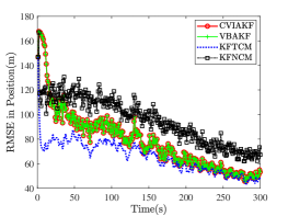
(a) RMSE in position

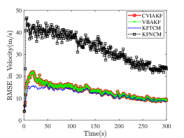
(b) RMSE in velocity

Figure 1: RMSE comparison for simulated scenario S1

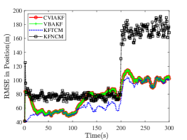
(a) RMSE in position

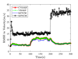
(b) RMSE in velocity

Figure 2: RMSE comparison for simulated scenario S2

TABLE II: ARMSE comparison for linear scenarios

Scenarios	S1		S2
Methods	Position	Velocity	Position	Velocity
KFNCM	95.21	32.79	108.54	21.18
VBAKF	79.01	13.27	78.24	7.74
CVIAKF	79.01	13.27	78.24	7.74
KFTCM	65.34	12.07	69.87	7.19

The RMSEs comparison for nonlinear scenarios S3 and S4 are shown in Fig. 3 and Fig. 5, respectively. It is shown that CVIAKF outperforms existing VB-based adaptive filters. This is because both CVIAKF and VBAKF-CM estimate the unknown $\bm{Q}_{k}$ and $\bm{R}_{k}$, which is better than VBACIF estimating only $\bm{R}_{k}$ and SSVBAKF estimating only $\bm{Q}_{k}$. Meanwhile, CVIAKF directly optimizes the non-conjugate ELBO via the stochastic mirror gradient descent method. VBAKF-CM carries out the nonlinear adaptive filtering into two subproblems: linear approximation based on unbiased measurement conversion and linear adaptive filtering. In cases where the measurement noise covariance $\bm{R}_{k}$ is unknown, there may be significant errors in the conversion process. Table.III illustrates the ARMSE comparison for different methods, indicating that CVIAKF is the best, followed by VBAKF-CM and SSVBAKF, and VBACIF is the worst. All comparison methods are based on VB. The average iterations of VBACIF, VBAKF-CM, SSVBAKF and CVIAKF are 5, 9, 120, 27 for scenario S3, and 5, 8, 68, 24 for scenario S4, respectively. The fast convergence of VBACIF and VBAKF-CM can be attributed to their use of conjugate computations. On the other hand, SSVBAKF and CVIAKF require more iterations to update their hyperparameters since they rely on stochastic gradient optimization. However, CVIAKF uses stochastic mirror gradient descent to accelerate the convergence of stochastic gradient descent, which ultimately results in fewer iterations than SSVBAKF.

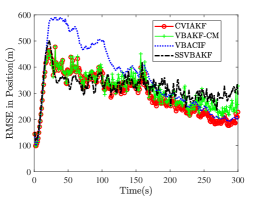
(a) RMSE in position

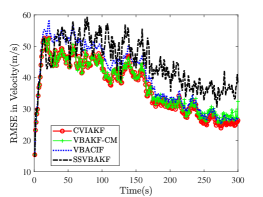
(b) RMSE in velocity

Figure 3: RMSE comparison for simulated scenario S3

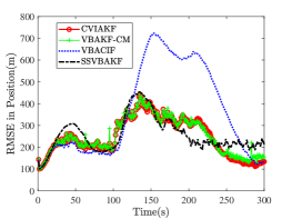
(a) RMSE in position

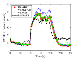
(b) RMSE in velocity

Figure 4: RMSE comparison for simulated scenario S4

TABLE III: ARMSE comparison for nonlinear scenarios

Scenarios	S3		S4
Methods	Position	Velocity	Position	Velocity
VBACIF	363.55	40.46	362.55	23.71
SSVBAKF	322.78	44.72	256.51	21.61
VBAKF-CM	314.71	37.59	250.52	21.52
CVIAKF	295.19	37.03	245.84	21.32

V Results For Real-World Data

Three different maneuvering target tracking applications with real-world 2D surveillance radar datasets are used to evaluate the performance of different VB-based adaptive filtering methods.

• R1[23]: The aerial target trajectory is shown in Fig. 5a, which consists of six different segments or maneuver modes. These segments include segment-A (CV), segment-B (left CT), segment C (CV), segment D (right CT), segment E (CA), and segment-F (figure-eight flight pattern).

• R2[23]: The vehicle target trajectory is shown in Fig. 5b which consists of round-trip maneuver.

• R3[23]: The ship target trajectory is shown in Fig. 5c which consists of coordinated turn maneuver.

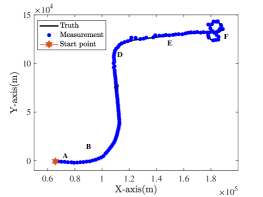
(a) R1

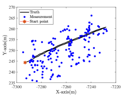
(b) R2

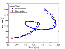
(c) R3

Figure 5: Trajectories of targets and radar measurements in real-world scenarios.

The radar sampling period $T$ for R1, R2, and R3 are 10s, 2s, and 3s, respectively. The algorithms are configured with the same parameters as the synthetic data scenarios. The results are shown as follows. Fig.6 and Table.IV depict the RMSE and ARMSE for different real-world datasets, respectively. It is seen that CVIAKF has the best tracking performance for all real scenarios, followed by SSVBAKF and VBAKF-CM, and VBACIF is the worst. In particular, Fig. 6a and Table. V show the segment analysis of RMSE for scenario R1. When the target moves with CV modes or with small turning maneuvers, all adaptive Kalman filtering methods perform well. However, VBAEKF-CM and CVIAKF have proven to be the most effective. When the target executes a large turning maneuver (segments D and F) or experiences acceleration (segment E), the filtering performance of all methods degrades. Nonetheless, CVIAKF exhibits relatively robust performance for different maneuvers. In contrast to scenario R1, the targets in scenarios R2 and R3 exhibit a more consistent movement pattern characterized by straight lines or turns. In these scenarios, all adaptive Kalman filtering methods can produce satisfactory estimation results. The average iterations for VBACIF, VBAKF-CM, SSVBAKF, and CVIAKF are 5, 5, 914, 183 for scenario R1, 4, 3, 6, 14 for scenario R2, and 5, 6, 590, 180 for scenario R3, respectively.

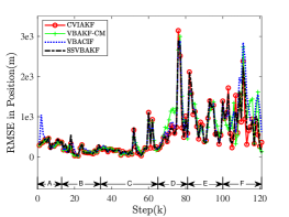
(a) R1

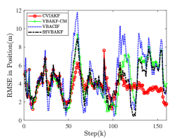
(b) R2

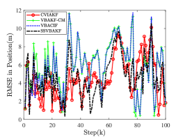
(c) R3

Figure 6: Position RSME comparison for real-world scenarios

TABLE IV: ARMSE comparison of positions for real-world scenarios (units: m)

Scenario	VBACIF	VBAKF-CM	SSVBAKF	CVIAKF
R1	628.10	597.52	548.25	531.54
R2	4.72	4.38	4.22	3.71
R3	5.80	5.96	4.64	4.42

TABLE V: ARMSE comparison of positions of different segments for scenario R1 (units: m)

Segment	VBACIF	VBAKF-CM	SSVBAKF	CVIAKF
A : [0, 13)	419.99	341.10	361.40	346.06
B : [13, 34)	186.07	156.18	177.24	159.45
C : [34, 65)	237.36	238.56	234.03	226.87
D : [65, 81)	943.45	1077.90	835.06	840.71
E : [81, 100)	877.71	908.06	904.38	893.37
F : [100, 121]	1269.20	1046.80	930.95	878.05

VI Conclusion

We have proposed CVIAKF for both linear and nonlinear state space models. Unlike the existing adaptive Kalman filters that directly apply variational inference in natural-parameter space, CVIAKF conducts optimization in the expectation-parameter space, leading to a faster and simpler solution, especially for nonlinear state estimation. Meanwhile, CVIAKF divides the ELBO optimization into conjugate parts and non-conjugate parts for nonlinear dynamic models, for which the conjugate computations and stochastic mirror-descent are applied, respectively. The reparameterization trick is used to reduce the variance of stochastic gradients of the non-conjugate parts, which can further improve the estimation accuracy. The positive-definite constraint in the stochastic mirror-descent method has been considered for enhancing numerical stability. The CVIAKF method has been validated with synthetic and real-world datasets for maneuvering target tracking.

APPENDIX A

For linear models, the updates of natural parameters $\bm{\lambda}_{k}^{\bm{x}}$, $\bm{\lambda}_{k}^{\bm{P}}$ and $\bm{\lambda}_{k}^{\bm{R}}$ can be obtained directly by setting the deviations of ELBO $\mathcal{\bar{B}}(\bm{\mu}_{k})$ equal to zeros. For simplicity, here and thereafter, we denote the expectation $\mathbb{E}_{q(\bm{x})}[\bm{x}]$ as $\mathbb{E}[\bm{x}]$.

$$\begin{split}\mathcal{\bar{B}}(\bm{\mu}_{k}^{\bm{x}})=&\mathbb{E}\left[-0.5(\bm{y}_{k}-\bm{H}_{k}\bm{x}_{k})^{\top}\bm{R}_{k}^{-1}(\bm{y}_{k}-\bm{H}_{k}\bm{x}_{k})\right]+\mathbb{E}\left[-0.5(\bm{x}_{k}-\hat{\bm{x}}_{k|k-1})^{\top}\bm{P}_{k|k-1}^{-1}(\bm{x}_{k}-\hat{\bm{x}}_{k|k-1})\right]\\ &-\mathbb{E}\left[-0.5(\bm{x}_{k}-\hat{\bm{x}}_{k|k})^{\top}\bm{P}_{k|k}^{-1}(\bm{x}_{k}-\hat{\bm{x}}_{k|k})\right]\\ =&\mathrm{Tr}\left\{\big{(}\bm{H}_{k}^{\top}\mathbb{E}[\bm{R}_{k}^{-1}]\bm{y}_{k}+\mathbb{E}[\bm{P}_{k|k-1}^{-1}]\hat{\bm{x}}_{k|k-1}-\bm{P}_{k|k}^{-1}\hat{\bm{x}}_{k|k}\big{)}(\bm{\mu}_{k}^{\bm{x}}(1))^{\top}\right\}\\ &-0.5\mathrm{Tr}\left\{\big{(}\bm{H}_{k}^{\top}\mathbb{E}[\bm{R}_{k}^{-1}]\bm{H}_{k}+\mathbb{E}[\bm{P}_{k|k-1}^{-1}]-\bm{P}_{k|k}^{-1}\big{)}\bm{\mu}_{k}^{\bm{x}}(2)\right\}\end{split}$$ (33)

1. Derivations of $\bm{\lambda}_{k}^{\bm{x}}$: Omitting the terms that are independent of $\bm{x}_{k}$, the simplified ELBO $\mathcal{\bar{B}}(\bm{\mu}_{k})$, denoted by $\mathcal{\bar{B}}(\bm{\mu}_{k}^{\bm{x}})$, can be written as (33), where $\bm{\mu}_{k}^{\bm{x}}(1)=\mathbb{E}[\bm{x}_{k}]$ and $\bm{\mu}_{k}^{\bm{x}}(2)=\mathbb{E}[\bm{x}_{k}\bm{x}_{k}^{\top}]$.

Let the gradients of (33) w.r.t. $\bm{\mu}_{k}^{\bm{x}}$ be equal to zeros, the variational parameters $\bm{\hat{x}}_{k}$ and $\bm{P}_{k|k}$ can be updated as

$$\begin{split}\bm{P}_{k|k}^{-1}\hat{\bm{x}}_{k|k}=\,&\mathbb{E}[\bm{P}_{k|k-1}^{-1}]\hat{\bm{x}}_{k|k-1}+\bm{H}_{k}^{\top}\mathbb{E}[\bm{R}_{k}^{-1}]\bm{y}_{k},\\ \bm{P}_{k|k}^{-1}=\,&\mathbb{E}[\bm{P}_{k|k-1}^{-1}]+\bm{H}_{k}^{\top}\mathbb{E}[\bm{R}_{k}^{-1}]\bm{H}_{k}.\end{split}$$ (31)

$$\begin{split}\mathcal{\bar{B}}(\bm{\mu}_{k}^{\bm{P}})=&\mathbb{E}\left[-0.5(\bm{x}_{k}-\hat{\bm{x}}_{k|k-1})^{\top}\bm{P}_{k|k-1}^{-1}(\bm{x}_{k}-\hat{\bm{x}}_{k|k-1})-0.5\log\left|\bm{P}_{k|k-1}\right|\right]\\ &+\mathbb{E}\left[-0.5(\hat{u}_{k|k-1}+n+1)\log\left|\bm{P}_{k|k-1}\right|-0.5\mathrm{Tr}\{\bm{U}_{k|k-1}\bm{P}_{k|k-1}^{-1}\}\right]\\ &+\mathbb{E}\left[0.5(\hat{u}_{k|k}+n+1)\log\left|\bm{P}_{k|k-1}\right|+0.5\mathrm{Tr}\{\bm{U}_{k|k}\bm{P}_{k|k-1}^{-1}\}\right]\\ &=0.5(\hat{u}_{k|k}-\hat{u}_{k|k-1}-1)\bm{\mu}_{k}^{\bm{P}}(1)+0.5\mathrm{Tr}\left\{\left(\bm{U}_{k|k}-\bm{C}_{k}-\bm{U}_{k|k-1}\right)\bm{\mu}_{k}^{\bm{P}}(2)\right\}\end{split}$$ (35)

2. Derivations of $\bm{\lambda}_{k}^{\bm{P}}$: Omitting the terms that are independent of $\bm{P}_{k|k-1}$, the simplified ELBO $\mathcal{\bar{B}}(\bm{\mu}_{k})$, denoted by $\mathcal{\bar{B}}(\bm{\mu}_{k}^{\bm{P}})$, can be written as (35), where $\bm{\mu}_{k}^{\bm{P}}(1)=\mathbb{E}[\log|\bm{P}_{k|k-1}|]$, $\bm{\mu}_{k}^{\bm{P}}(2)=\mathbb{E}[\bm{P}_{k|k-1}^{-1}]$, and $\bm{C}_{k}\triangleq\mathbb{E}[(\bm{x}_{k}-\hat{\bm{x}}_{k|k-1})(\bm{x}_{k}-\hat{\bm{x}}_{k|k-1})^{\top}]=(\hat{\bm{x}}_{k|k}-\hat{\bm{x}}_{k|k-1})(\hat{\bm{x}}_{k|k}-\hat{\bm{x}}_{k|k-1})^{\top}+\bm{P}_{k|k}$.

Let the gradients of (35) w.r.t. $\bm{\mu}_{k}^{\bm{P}}$ be equal to zeros, the variational parameters $u_{k|k}$ and $\bm{U}_{k|k}$ can be updated as

$$\begin{split}\hat{u}_{k|k}=&\hat{u}_{k|k-1}+1,\\ \bm{U}_{k|k}=&\bm{U}_{k|k-1}+\bm{C}_{k}.\end{split}$$ (33)

3. Derivations of $\bm{\lambda}_{k}^{\bm{R}}$: Omitting the terms that are independent of $\bm{R}_{k}$, the simplified ELBO $\mathcal{\bar{B}}(\bm{\mu}_{k})$, denoted by $\mathcal{\bar{B}}(\bm{\mu}_{k}^{\bm{R}})$, can be written as (37), where $\bm{\mu}_{k}^{\bm{R}}(1)=\mathbb{E}[\log|\bm{R}_{k}|]$, $\bm{\mu}_{k}^{\bm{R}}(2)=\mathbb{E}[\bm{R}_{k}^{-1}]$, and $\bm{A}_{k}\triangleq\mathbb{E}[(\bm{y}_{k}-\bm{H}_{k}\bm{x}_{k})(\bm{y}_{k}-\bm{H}_{k}\bm{x}_{k})^{\top}]=(\bm{y}_{k}-\bm{H}_{k}\hat{\bm{x}}_{k|k})(\bm{y}_{k}-\bm{H}_{k}\hat{\bm{x}}_{k|k})^{\top}+\bm{H}_{k}\bm{P}_{k|k}\bm{H}_{k}^{\top}$.

$$\begin{split}\mathcal{\bar{B}}(\bm{\mu}_{k}^{\bm{R}})=&\mathbb{E}\left[-0.5(\bm{y}_{k}-\bm{H}_{k}\bm{x}_{k})^{\top}\bm{R}_{k}^{-1}(\bm{y}_{k}-\bm{H}_{k}\bm{x}_{k})-0.5\log\left|\bm{R}_{k}\right|\right]\\ &-\mathbb{E}\left[0.5(\hat{v}_{k|k-1}+m+1)\log\left|\bm{R}_{k}\right|+0.5\mathrm{Tr}\{\bm{V}_{k|k-1}\bm{R}_{k}^{-1}\}\right]\\ &+\mathbb{E}\left[0.5(\hat{v}_{k|k}+m+1)\log\left|\bm{R}_{k}\right|+0.5\mathrm{Tr}\{\bm{V}_{k|k}\bm{R}_{k}^{-1}\}\right]\\ =&0.5(\hat{v}_{k|k}-\hat{v}_{k|k-1}-1)\bm{\mu}_{k}^{\bm{R}}(1)+0.5\mathrm{Tr}\left\{\left(\bm{V}_{k|k}-\bm{A}_{k}-\bm{V}_{k|k-1}\right)\bm{\mu}_{k}^{\bm{R}}(2)\right\}\end{split}$$ (37)

Let the gradients of (37) w.r.t. $\bm{\mu}_{k}^{\bm{R}}$ be equal to zeros, the variational parameters $v_{k|k}$ and $\bm{V}_{k|k}$ can be updated as

$$\begin{split}\hat{v}_{k|k}=&\hat{v}_{k|k-1}+1,\\ \bm{V}_{k|k}=&\bm{V}_{k|k-1}+\bm{A}_{k}.\end{split}$$ (35)

The proof of Theorem 1 has been completed. $\hfill\Large\square$

APPENDIX B

For linear models, the update of the natural parameters $\bm{\lambda}_{k}^{x}$ (24) can be simplified as

$$\bm{P}_{k|k}^{-1}=\, \mathbb{E}[\bm{P}_{k|k-1}^{-1}]+\bm{H}_{k}^{\top}\mathbb{E}[\bm{R}_{k}^{-1}]\bm{H}_{k},$$ (36)

$$\hat{\bm{x}}_{k|k}=\, \bm{P}_{k|k}\left[\mathbb{E}[\bm{P}_{k|k-1}^{-1}]\hat{\bm{x}}_{k|k-1}+\bm{H}_{k}^{\top}\mathbb{E}[\bm{R}_{k}^{-1}]\bm{y}_{k}\right].$$ (37)

Inverting both sides of (36) and employing the Sherman-Morrison-Woodbury Lemma, we have

$$\begin{split}\bm{P}_{k|k}=\,&\left[\mathbb{E}[\bm{P}_{k|k-1}^{-1}]+\bm{H}_{k}^{\top}\mathbb{E}[\bm{R}_{k}^{-1}]\bm{H}_{k}\right]^{-1}\\ =\,&\tilde{\bm{P}}_{k|k-1}-\bm{K}_{k}\bm{H}_{k}\tilde{\bm{P}}_{k|k-1}\\ =\,&(\bm{\mathrm{I}}_{n}-\bm{K}_{k}\bm{H}_{k})\tilde{\bm{P}}_{k|k-1}\end{split}$$ (38)

with $\tilde{\bm{P}}_{k|k-1}^{-1}\triangleq\mathbb{E}[\bm{P}_{k|k-1}^{-1}]$, $\tilde{\bm{R}}_{k}^{-1}\triangleq\mathbb{E}[\bm{R}_{k}^{-1}]$, and the filter gain $\bm{K}_{k}=\tilde{\bm{P}}_{k|k-1}\bm{H}_{k}^{\top}(\tilde{\bm{R}}_{k}+\bm{H}_{k}\tilde{\bm{P}}_{k|k-1}\bm{H}_{k}^{\top})^{-1}$.

By the fact that the following equation holds

$$\begin{split}\bm{K}\tilde{\bm{R}}_{k}=\,&\bm{K}(\tilde{\bm{R}}_{k}+\bm{H}_{k}\tilde{\bm{P}}_{k|k-1}\bm{H}^{\top})-\bm{K}\bm{H}_{k}\tilde{\bm{P}}_{k|k-1}\bm{H}_{k}^{\top}\\ =\,&\tilde{\bm{P}}_{k|k-1}\bm{H}_{k}^{\top}-\bm{K}\bm{H}_{k}\tilde{\bm{P}}_{k|k-1}\bm{H}_{k}^{\top}\\ =\,&(\bm{\mathrm{I}}_{n}-\bm{K}\bm{H}_{k})\tilde{\bm{P}}_{k|k-1}\bm{H}_{k}^{\top}\\ =\,&\bm{P}_{k|k}\bm{H}_{k}^{\top},\end{split}$$ (39)

the filter gain can be rewritten as $\bm{K}=\bm{P}_{k|k}\bm{H}_{k}^{\top}\tilde{\bm{R}}_{k}^{-1}$.

Therefore, (37) can be expressed as

$$\begin{split}\hat{\bm{x}}_{k|k}=\,&\bm{P}_{k|k}\tilde{\bm{P}}_{k|k-1}^{-1}\hat{\bm{x}}_{k|k-1}+\bm{P}_{k|k}\bm{H}_{k}^{\top}\tilde{\bm{R}}_{k}^{-1}\bm{y}_{k}\\ =\,&\hat{\bm{x}}_{k|k-1}-\bm{K}\bm{H}_{k}\hat{\bm{x}}_{k|k-1}+\bm{K}\bm{y}_{k}\\ =\,&\hat{\bm{x}}_{k|k-1}+\bm{K}(\bm{y}_{k}-\bm{H}_{k}\hat{\bm{x}}_{k|k-1}).\end{split}$$ (40)

From the proof of Theorem 1, the updated natural parameters of $\bm{P}_{k|k-1}$ and $\bm{R}_{k}$ can be simplified as (33) and (35), respectively. Combining (38) with (40), it is demonstrated that CVIAKF is equivalent to VBAKF.

When $\bm{Q}_{k}$ and $\bm{R}_{k}$ are known, the predicted state $\bm{P}_{k|k-1}$ and $\bm{R}_{k}$ can be obtained accurately. Then, $\mathbb{E}[\bm{P}_{k|k-1}^{-1}]=\bm{P}_{k|k-1}^{-1}$ and $\mathbb{E}[\bm{R}_{k}^{-1}]=\bm{R}_{k}^{-1}$. The updated natural parameters $\bm{\lambda}_{k}^{x}$ (24) can be simplified as

$$\begin{split}\bm{P}_{k|k}^{-1}=\,&\bm{P}_{k|k-1}^{-1}+\bm{H}_{k}^{\top}\bm{R}_{k}^{-1}\bm{H}_{k},\\ \bm{P}_{k|k}^{-1}\hat{\bm{x}}_{k|k}=\,&\bm{P}_{k|k-1}^{-1}\hat{\bm{x}}_{k|k-1}+\bm{H}_{k}^{\top}\bm{R}_{k}^{-1}\bm{y}_{k}.\end{split}$$ (41)

The update of simplified parameters (41) is a standard information filter, where $\bm{P}_{k|k}^{-1}$ and $\bm{P}_{k|k}^{-1}\hat{\bm{x}}_{k|k}$ are respectively defined as the information matrix and information vector. The predicted information matrix and predicted information vector are $\bm{P}_{k|k-1}^{-1}$ and $\bm{P}_{k|k-1}^{-1}\hat{\bm{x}}_{k|k-1}$. The measurement covariance is $\bm{H}_{k}^{\top}\bm{R}_{k}^{-1}\bm{H}_{k}$, and the measurement vector is $\bm{H}_{k}^{\top}\bm{R}_{k}^{-1}\bm{y}_{k}$.

The proof of Proposition 1 has been completed. $\hfill\Large\square$

APPENDIX C

For nonlinear models, it is intractable to optimize the ELBO objective directly. One should resort to the stochastic mirror descent method.

$$\begin{split}\mathcal{\bar{B}}(\bm{\mu}_{k}^{\bm{x}})=&-0.5\underbrace{\mathbb{E}\left[(\bm{y}_{k}-\bm{h}_{k}(\bm{x}_{k}))^{\top}\bm{R}_{k}^{-1}(\bm{y}_{k}-\bm{h}_{k}(\bm{x}_{k}))\right]}_{\mathcal{D}(\bm{\mu}_{k}^{\bm{x}})}\\ &-0.5\underbrace{\mathbb{E}\left[(\bm{x}_{k}-\hat{\bm{x}}_{k|k-1})^{\top}\bm{P}_{k|k-1}^{-1}(\bm{x}_{k}-\hat{\bm{x}}_{k|k-1})-(\bm{x}_{k}-\hat{\bm{x}}_{k|k})^{\top}\bm{P}_{k|k}^{-1}(\bm{x}_{k}-\hat{\bm{x}}_{k|k})\right]}_{\mathcal{E}(\bm{\mu}_{k}^{\bm{x}})}\end{split}$$ (45)

1. Derivations of $\bm{\lambda}_{k}^{\bm{x}}$: Omitting the terms that are independent of $\bm{x}_{k}$, the simplified ELBO $\mathcal{\bar{B}}(\bm{\mu}_{k})$, denoted by $\mathcal{\bar{B}}(\bm{\mu}_{k}^{\bm{x}})$, can be written as (45), where $\mathcal{E}(\bm{\mu}_{k}^{\bm{x}})$ and $\mathcal{D}(\bm{\mu}_{k}^{\bm{x}})$ are the conjugate part and non-conjugate part of $\mathcal{\bar{B}}(\bm{\mu}_{k}^{\bm{x}})$, respectively.

The gradient of the ELBO $\mathcal{\bar{B}}(\bm{\mu}_{k}^{\bm{x}})$ w.r.t. expectation parameters $\bm{\mu}_{k}^{\bm{x}}$ can be expressed as

$$\nabla_{\bm{\mu}_{k}^{\bm{x}}}\mathcal{\bar{B}}(\bm{\mu}_{k}^{\bm{x}})=-0.5\nabla_{\bm{\mu}_{k}^{\bm{x}}}\mathcal{E}(\bm{\mu}_{k}^{\bm{x}})-0.5\nabla_{\bm{\mu}_{k}^{\bm{x}}}\mathcal{D}(\bm{\mu}_{k}^{\bm{x}}).$$ (43)

$$\begin{split}\nabla_{\bm{\mu}_{k}^{\bm{x}}}\mathcal{E}(\bm{\mu}_{k}^{\bm{x}})=\nabla_{\bm{\mu}_{k}^{\bm{x}}}\mathrm{Tr}\left\{2\big{(}-\mathbb{E}[\bm{P}_{k|k-1}^{-1}]\hat{\bm{x}}_{k|k-1}+\bm{P}_{k|k}^{-1}\hat{\bm{x}}_{k|k}\big{)}(\bm{\mu}_{k}^{\bm{x}}(1))^{\top}\right\}+\nabla_{\bm{\mu}_{k}^{\bm{x}}}\mathrm{Tr}\left\{\big{(}\mathbb{E}[\bm{P}_{k|k-1}^{-1}]-\bm{P}_{k|k}^{-1}\big{)}\bm{\mu}_{k}^{\bm{x}}(2)\right\}\end{split}$$ (47)

For the conjugate part $\mathcal{E}(\bm{\mu}_{k}^{\bm{x}})$, its gradient can be computed as (47), where $\bm{\mu}_{k}^{\bm{x}}=[\bm{\mu}_{k}^{\bm{x}}(1),\bm{\mu}_{k}^{\bm{x}}(2)]^{\top}$ with $\bm{\mu}_{k}^{\bm{x}}(1)=\mathbb{E}[\bm{x}_{k}]$ and $\bm{\mu}_{k}^{\bm{x}}(2)=\mathbb{E}[\bm{x}_{k}\bm{x}_{k}^{\top}]$. Then, the gradient of conjugate part $\nabla_{\bm{\mu}_{k}^{\bm{x}}}\mathcal{E}(\bm{\mu}_{k}^{\bm{x}})$ can be calculated in analytical form as

$$\begin{split}\nabla_{\bm{\mu}_{k}^{\bm{x}}(1)}\mathcal{E}(\bm{\mu}_{k}^{\bm{x}})=\,&-2\mathbb{E}[\bm{P}_{k|k-1}^{-1}]\hat{\bm{x}}_{k|k-1}+2\bm{P}_{k|k}^{-1}\hat{\bm{x}}_{k|k},\\ \nabla_{\bm{\mu}_{k}^{\bm{x}}(2)}\mathcal{E}(\bm{\mu}_{k}^{\bm{x}})=\,&\mathbb{E}[\bm{P}_{k|k-1}^{-1}]-\bm{P}_{k|k}^{-1}.\end{split}$$ (45)

$$\begin{split}\nabla_{\bm{\mu}_{k}^{\bm{x}}}\mathcal{D}(\bm{\mu}_{k}^{\bm{x}})=\nabla_{\bm{\mu}_{k}^{\bm{x}}}\mathrm{Tr}\left\{\mathbb{E}\left[\bm{R}_{k}^{-1}\right]\mathbb{E}\left[(\bm{y}_{k}-\bm{h}_{k}(\bm{x}_{k}))(\bm{y}_{k}-\bm{h}_{k}(\bm{x}_{k}))^{\top}\right]\right\}\end{split}$$ (49)

For the non-conjugate part $\mathcal{D}(\bm{\mu}_{k}^{\bm{x}})$, its gradient can be computed as (49). It is intractable to calculate the above gradient due to the nonlinear measurement function $\bm{h}_{k}(\bm{x}_{k})$. By using the chain rule, the gradient w.r.t. multivariate Gaussian distribution $\bm{x}_{k}\sim\bm{\mathrm{N}}(\bm{x}_{k}|\bm{\hat{x}}_{k|k},\bm{P}_{k|k})$ can be rewritten as

$$\begin{split}\nabla_{\bm{\mu}_{k}^{\bm{x}}(1)}\mathcal{D}(\bm{\mu}_{k}^{\bm{x}})=\,&\nabla_{\hat{\bm{x}}_{k|k}}\mathcal{D}(\bm{\mu}_{k}^{\bm{x}})-2\nabla_{\bm{P}_{k|k}}\mathcal{D}(\bm{\mu}_{k}^{\bm{x}})\hat{\bm{x}}_{k|k},\\ \nabla_{\bm{\mu}_{k}^{\bm{x}}(2)}\mathcal{D}(\bm{\mu}_{k}^{\bm{x}})=&\nabla_{\bm{P}_{k|k}}\mathcal{D}(\bm{\mu}_{k}^{\bm{x}}).\end{split}$$ (47)

Let $\varphi(\bm{x}_{k})=(\bm{y}_{k}-\bm{h}_{k}(\bm{x}_{k}))^{\top}\bm{R}_{k}^{-1}(\bm{y}_{k}-\bm{h}_{k}(\bm{x}_{k}))$. Using the Monte Carlo integration, and Bonnet’s theorem and Price’s theorem [33], the gradients in (47) can be approximated by (51)-(52), where $\bm{x}_{k}^{s}\overset{\mathrm{iid}}{\sim}\bm{\mathrm{N}}(\bm{x}_{k}|\bm{\hat{x}}_{k|k},\bm{P}_{k|k})$, $s=1,2,\cdots,S$ are the sampling particles with $S$ being the number of samples. $\bm{H}_{k}(\bm{x}_{k})\in\mathbb{R}^{m\times n}$ denotes the Jacobian matrix of $\bm{h}_{k}(\bm{x}_{k})$. Let $\mathcal{H}_{i}(\bm{x}_{k})\in\mathbb{R}^{1\times n}$ denote the $i$th row of $\bm{H}_{k}(\bm{x}_{k})$, then $\bm{G}_{i}(\bm{x}_{k})\in\mathbb{R}^{n\times n}$ is the Jacobian matrix of $\mathcal{H}_{i}(\bm{x}_{k})$. $B_{i}(\bm{x}_{k})$ denotes the $i$th element of the vector $\bm{R}_{k}^{-1}(\bm{y}_{k}-\bm{h}_{k}(\bm{x}_{k}))$.

$$\begin{split}\nabla_{\hat{\bm{x}}_{k|k}}\mathcal{D}(\bm{\mu}_{k}^{\bm{x}})=\mathbb{E}\left[\nabla_{\bm{x}_{k}}\varphi(\bm{x}_{k})\right]=-2\mathbb{E}\left[\bm{H}^{\top}_{k}(\bm{x}_{k})\bm{R}_{k}^{-1}(\bm{y}_{k}-\bm{h}_{k}(\bm{x}_{k}))\right]\approx-\frac{2}{S}\sum_{s=1}^{S}\bm{H}^{\top}_{k}(\bm{x}_{k}^{s})\mathbb{E}[\bm{R}_{k}^{-1}](\bm{y}_{k}-\bm{h}_{k}(\bm{x}_{k}^{s}))\end{split}$$ (51)

$$\begin{split}\nabla_{\bm{P}_{k|k}}\mathcal{D}(\bm{\mu}_{k}^{\bm{x}})=&0.5\mathbb{E}\left[\nabla^{2}_{\bm{x}_{k}}\varphi(\bm{x}_{k})\right]=\mathbb{E}\left[\bm{H}^{\top}_{k}(\bm{x}_{k})\bm{R}_{k}^{-1}\bm{H}_{k}(\bm{x}_{k})-\sum_{i=1}^{m}\bm{G}_{i}^{\top}(\bm{x}_{k})B_{i}(\bm{x}_{k})\right]\\ \approx&\frac{1}{S}\sum_{s=1}^{S}\left[\bm{H}^{\top}_{k}(\bm{x}_{k}^{s})\mathbb{E}[\bm{R}_{k}^{-1}]\bm{H}_{k}(\bm{x}_{k}^{s})-\sum_{i=1}^{m}\bm{G}_{i}^{\top}(\bm{x}^{s}_{k})B_{i}(\bm{x}^{s}_{k})\right]\end{split}$$ (52)

In practice, the gradients in (51)-(52) approximated by Monte Carlo integration may have high variance. To address this issue, we employ the reparameterization trick [34] to reduce the estimation variance.

Assume that the random variable $\bm{x}_{k}$ can be expressed as the noise term $\bm{\epsilon}$ and deterministic terms $\bm{\theta}_{k}$, the reparameterization trick involves sampling from a noise distribution $q_{0}(\bm{\epsilon}_{k})$, which is independent of $\bm{\theta}_{k}$, and subsequently transforming to $\bm{x}_{k}$ through a deterministic and differentiable function $\bm{x}_{k}=\bm{g}(\bm{\epsilon}_{k})$. For Gaussian random variable $\bm{x}_{k}$, instead of sampling $\bm{x}_{k}\sim\bm{\mathrm{N}}(\bm{x}_{k}|\bm{\hat{x}}_{k|k},\bm{P}_{k|k})$, we can sample $\bm{\epsilon}_{k}\sim\bm{\mathrm{N}}(\bm{\mathrm{0}},\bm{\mathrm{I}}_{n})$ and compute $\bm{x}_{k}=\bm{g}(\bm{\epsilon}_{k})=\hat{\bm{x}}_{k|k}+\bm{L}_{k}\bm{\epsilon}_{k}$ with $\bm{L}_{k}\bm{L}_{k}^{\top}=\bm{P}_{k|k}$. Then, the reparameterization gradients are computed by

$$\begin{split}\nabla_{\hat{\bm{x}}_{k|k}}\mathcal{D}(\bm{\mu}_{k}^{\bm{x}})=&\mathbb{E}\left[\nabla_{\bm{g}(\bm{\epsilon}_{k})}\varphi(\bm{x}_{k})\nabla_{\hat{\bm{x}}_{k|k}}\bm{g}(\bm{\epsilon}_{k})\right]\\ =&-2\mathbb{E}\left[\bm{H}^{\top}_{k}(\bm{x}_{k})\bm{R}_{k}^{-1}(\bm{y}_{k}-\bm{h}_{k}(\bm{x}_{k}))\right]\\ \approx&-\frac{2}{S}\sum_{s=1}^{S}\bm{H}^{\top}_{k}(\bm{g}(\bm{\epsilon}_{k}^{s}))\mathbb{E}[\bm{R}_{k}^{-1}](\bm{y}_{k}-\bm{h}_{k}(\bm{\epsilon}_{k}^{s})),\end{split}$$ (50)

and

$$\begin{split}\nabla_{\bm{P}_{k|k}}\mathcal{D}(\bm{\mu}_{k}^{\bm{x}})=&\mathbb{E}\left[\nabla_{\bm{g}(\bm{\epsilon}_{k})}\varphi(\bm{x}_{k})\nabla_{\bm{P}_{k|k}}\bm{g}(\bm{\epsilon}_{k})\right]\\ \approx&-\frac{1}{S}\sum_{s=1}^{S}\bm{H}^{\top}_{k}(\bm{g}(\bm{\epsilon}_{k}^{s}))\mathbb{E}[\bm{R}_{k}^{-1}]\\ &\times(\bm{y}_{k}-\bm{h}_{k}(\bm{g}(\bm{\epsilon}_{k}^{s})))(\bm{\epsilon}_{k}^{s})^{\top}\bm{L}_{k}^{-1}.\end{split}$$ (51)

Based on the stochastic mirror descent method, the natural parameters of $\bm{x}_{k}$ can be updated iteratively as

$$\begin{split}(-0.5\bm{P}_{k|k}^{-1})^{(r+1)}=&(-0.5\bm{P}_{k|k}^{-1})^{(r)}+\beta_{k}^{(r)}\nabla_{\bm{\mu}_{k}^{\bm{x}}{(2)}}\mathcal{\bar{B}}(\bm{\mu}_{k}^{\bm{x}}),\\ (\bm{P}_{k|k}^{-1}\hat{\bm{x}}_{k|k})^{(r+1)}=&(\bm{P}_{k|k}^{-1}\hat{\bm{x}}_{k|k})^{(r)}+\beta_{k}^{(r)}\nabla_{\bm{\mu}_{k}^{\bm{x}}(1)}\mathcal{\bar{B}}(\bm{\mu}_{k}^{\bm{x}}),\end{split}$$ (52)

where $\beta_{k}^{(r)}$ is learning rate and $r$ is the iteration number.

Substituting the conjugate part in (45) and the non-conjugate part in (50)-(51) into (52), yields

$$\begin{split}(\bm{P}_{k|k}^{-1})^{(r+1)}=&(1-\beta_{k}^{(r)})(\bm{P}_{k|k}^{-1})^{(r)}\\ &+\beta_{k}^{(r)}\left(\mathbb{E}[\bm{P}_{k|k-1}^{-1}]+\nabla_{\bm{P}_{k|k}}\mathcal{D}(\bm{\mu}_{k}^{\bm{x}})\right),\end{split}$$ (53)

$$\begin{split}\hat{\bm{x}}_{k|k}^{(r+1)}=&\hat{\bm{x}}_{k|k}^{(r)}+\beta_{k}^{(r)}\bm{P}_{k|k}^{(r+1)}\mathbb{E}[\bm{P}_{k|k-1}^{-1}](\hat{\bm{x}}_{k|k-1}-\hat{\bm{x}}_{k|k}^{(r)})\\ &-0.5\beta_{k}^{(r)}\bm{P}_{k|k}^{(r+1)}\nabla_{\hat{\bm{x}}_{k|k}}\mathcal{D}(\bm{\mu}_{k}^{\bm{x}}).\end{split}$$ (54)

An issue with the above updates (53)-(54) is that the constraint is not taken into account. For multivariate Gaussian distribution, the covariance matrix $\bm{P}_{k|k}$ should be real-value and positive-definite. However, the learning rate $\beta_{k}^{(r)}$ in (53) does not ensure that $\bm{P}_{k|k}$ are always positive. Setting the learning rate $\beta_{k}^{(r)}$ too high can cause the CVIAKF algorithm to diverge, and too low makes it slow to converge.

To address this issue, one can use the line-search approach [30]. The constraint can be satisfied by adding a compensation term into Eq.(53), that is:

$$\begin{split}(\bm{P}_{k|k}^{-1})^{(r+1)}=&\frac{(\beta_{k}^{(r)})^{2}}{2}\hat{\bm{\mathrm{G}}}_{k}\bm{P}^{(r)}_{k|k}\hat{\bm{\mathrm{G}}}_{k}+(1-\beta_{k}^{(r)})(\bm{P}_{k|k}^{-1})^{(r)}\\ &+\beta_{k}^{(r)}\left(\mathbb{E}[\bm{P}_{k|k-1}^{-1}]+\nabla_{\bm{P}_{k|k}}\mathcal{D}(\bm{\mu}_{k}^{\bm{x}})\right)\end{split}$$ (55)

with

$$\hat{\bm{\mathrm{G}}}_{k}=(\bm{P}_{k|k}^{-1})^{(r)}-\left(\mathbb{E}[\bm{P}_{k|k-1}^{-1}]+\nabla_{\bm{P}_{k|k}}\mathcal{D}(\bm{\mu}_{k}^{\bm{x}})\right).$$ (56)

The update (55) can substantiate that $\bm{P}_{k|k}^{-1}$ is always positive-definite [30].

2. Derivations of $\bm{\lambda}_{k}^{\bm{P}}$: the update of natural parameter $\bm{\lambda}_{k}^{\bm{P}}$ is same as (33) since the measurement function $\bm{h}_{k}(\bm{x}_{k})$ has no relationship with (35).

3. Derivations of $\bm{\lambda}_{k}^{\bm{R}}$: the update of natural parameter $\bm{\lambda}_{k}^{\bm{R}}$ remains to be (35), whereas the term $\bm{A}_{k}$ is modified as

$$\begin{split}\bm{A}_{k}=\,&\mathbb{E}[(\bm{y}_{k}-\bm{h}_{k}(\bm{x}_{k}))(\bm{y}_{k}-\bm{h}_{k}(\bm{x}_{k}))^{\top}]\\ \approx\,&\frac{1}{S}\sum_{s=1}^{S}[(\bm{y}_{k}-\bm{h}_{k}(\hat{\bm{x}}_{k|k}+\bm{L}_{k}\bm{\epsilon}_{k}^{s}))(\cdot)^{\top}].\end{split}$$ (57)

The proof of Theorem 2 has been completed. $\hfill\Large\square$

References

- [1] N. H. Gholson and R. L. Moose, “Maneuvering target tracking using adaptive state estimation,” IEEE Transactions on Aerospace and Electronic Systems, no. 3, pp. 310–317, 1977.
- [2] K. Li, S. Zhao, C. K. Ahn, and F. Liu, “State estimation for jump Markov nonlinear systems of unknown measurement data covariance,” Journal of the Franklin Institute, vol. 358, no. 2, pp. 1673–1691, 2021.
- [3] X.-R. Li and Y. Bar-Shalom, “Multiple-model estimation with variable structure,” IEEE Transactions on Automatic control, vol. 41, no. 4, pp. 478–493, 1996.
- [4] H. A. Blom and Y. Bar-Shalom, “The interacting multiple model algorithm for systems with Markovian switching coefficients,” IEEE Transactions on Automatic Control, vol. 33, no. 8, pp. 780–783, 1988.
- [5] E. Mazor, A. Averbuch, Y. Bar-Shalom, and J. Dayan, “Interacting multiple model methods in target tracking: A survey,” IEEE Transactions on Aerospace and Electronic Systems, vol. 34, no. 1, pp. 103–123, 1998.
- [6] X. R. Li and V. P. Jilkov, “Survey of maneuvering target tracking: Decision-based methods,” in Signal and Data Processing of Small Targets 2002, vol. 4728. SPIE, 2002, pp. 511–534.
- [7] M. S. Arulampalam, S. Maskell, N. Gordon, and T. Clapp, “A tutorial on particle filters for online nonlinear/non-gaussian Bayesian tracking,” IEEE Transactions on Signal Processing, vol. 50, no. 2, pp. 174–188, 2002.
- [8] E. Özkan, V. Šmídl, S. Saha, C. Lundquist, and F. Gustafsson, “Marginalized adaptive particle filtering for nonlinear models with unknown time-varying noise parameters,” Automatica, vol. 49, no. 6, pp. 1566–1575, 2013.
- [9] D. M. Blei, A. Kucukelbir, and J. D. McAuliffe, “Variational inference: A review for statisticians,” Journal of the American Statistical Association, vol. 112, no. 518, pp. 859–877, 2017.
- [10] S. Sarkka and A. Nummenmaa, “Recursive noise adaptive Kalman filtering by variational Bayesian approximations,” IEEE Transactions on Automatic control, vol. 54, no. 3, pp. 596–600, 2009.
- [11] Y. Huang, Y. Zhang, Z. Wu, N. Li, and J. Chambers, “A novel adaptive Kalman filter with inaccurate process and measurement noise covariance matrices,” IEEE Transactions on Automatic Control, vol. 63, no. 2, pp. 594–601, 2018.
- [12] T. Ardeshiri, E. Özkan, U. Orguner, and F. Gustafsson, “Approximate Bayesian smoothing with unknown process and measurement noise covariances,” IEEE Signal Processing Letters, vol. 22, no. 12, pp. 2450–2454, 2015.
- [13] Y. Ma, S. Zhao, and B. Huang, “Multiple-model state estimation based on variational Bayesian inference,” IEEE Transactions on Automatic Control, vol. 64, no. 4, pp. 1679–1685, 2018.
- [14] F. Zhu, Y. Huang, C. Xue, L. Mihaylova, and J. Chambers, “A sliding window variational outlier-robust Kalman filter based on student’s t-noise modeling,” IEEE Transactions on Aerospace and Electronic Systems, vol. 58, no. 5, pp. 4835–4849, 2022.
- [15] X. Yu and Z. Meng, “Robust Kalman filters with unknown covariance of multiplicative noise,” IEEE Transactions on Automatic Control, pp. 1–8, 2023.
- [16] H. Xu, K. Duan, H. Yuan, W. Xie, and Y. Wang, “Adaptive fixed-lag smoothing algorithms based on the variational Bayesian method,” IEEE Transactions on Automatic Control, vol. 66, no. 10, pp. 4881–4887, 2020.
- [17] M. Xia, T. Zhang, J. Wang, L. Zhang, Y. Zhu, and L. Guo, “The fine calibration of the ultra-short baseline system with inaccurate measurement noise covariance matrix,” IEEE Transactions on Instrumentation and Measurement, vol. 71, pp. 1–8, 2021.
- [18] H. Zhu, G. Zhang, Y. Li, and H. Leung, “A novel robust Kalman filter with unknown non-stationary heavy-tailed noise,” Automatica, vol. 127, p. 109511, 2021.
- [19] ——, “An adaptive Kalman filter with inaccurate noise covariances in the presence of outliers,” IEEE Transactions on Automatic Control, vol. 67, no. 1, pp. 374–381, 2021.
- [20] I. S. Mbalawata, S. Sarkka, M. Vihola, and H. Haario, “Adaptive Metropolis algorithm using variational Bayesian adaptive Kalman filter,” Computational Statistics & Data Analysis, vol. 83, pp. 101–115, 2015.
- [21] P. Dong, Z. Jing, H. Leung, and K. Shen, “Variational Bayesian adaptive cubature information filter based on Wishart distribution,” IEEE Transactions on Automatic Control, vol. 62, no. 11, pp. 6051–6057, 2017.
- [22] M. D. Hoffman, D. M. Blei, C. Wang, and J. Paisley, “Stochastic variational inference,” Journal of Machine Learning Research, vol. 14, pp. 1303–1347, 2013.
- [23] H. Lan, J. Hu, Z. Wang, and Q. Cheng, “Variational nonlinear Kalman filtering with unknown process noise covariance,” IEEE Transactions on Aerospace and Electronic Systems, vol. 59, no. 6, pp. 9177–9190, 2023.
- [24] J. Martens, “New insights and perspectives on the natural gradient method,” The Journal of Machine Learning Research, vol. 21, no. 1, pp. 5776–5851, 2020.
- [25] J. Hensman, M. Rattray, and N. Lawrence, “Fast variational inference in the conjugate exponential family,” Advances in Neural Information Processing Systems, vol. 25, 2012.
- [26] W. Lin, M. E. Khan, and M. Schmidt, “Fast and simple natural-gradient variational inference with mixture of exponential-family approximations,” in International Conference on Machine Learning. PMLR, 2019, pp. 3992–4002.
- [27] M. Khan and W. Lin, “Conjugate-computation variational inference: Converting variational inference in non-conjugate models to inferences in conjugate models,” in Artificial Intelligence and Statistics. PMLR, 2017, pp. 878–887.
- [28] M. I. Skolnik, “Theoretical accuracy of radar measurements,” IRE Transactions on Aeronautical and Navigational Electronics, no. 4, pp. 123–129, 1960.
- [29] S. Gultekin and J. Paisley, “Nonlinear Kalman filtering with divergence minimization,” IEEE Transactions on Signal Processing, vol. 65, no. 23, pp. 6319–6331, 2017.
- [30] W. Lin, M. Schmidt, and M. E. Khan, “Handling the positive-definite constraint in the Bayesian learning rule,” in International Conference on Machine Learning. PMLR, 2020, pp. 6116–6126.
- [31] S. Bordonaro, P. Willett, and Y. Bar-Shalom, “Decorrelated unbiased converted measurement Kalman filter,” IEEE Transactions on Aerospace and Electronic Systems, vol. 50, no. 2, pp. 1431–1444, 2014.
- [32] Y. Huang, Y. Zhang, P. Shi, and J. Chambers, “Variational adaptive Kalman filter with Gaussian-inverse-Wishart mixture distribution,” IEEE Transactions on Automatic Control, vol. 66, no. 4, pp. 1786–1793, 2020.
- [33] K. P. Murphy, Probabilistic machine learning: Advanced topics. MIT press, 2023.
- [34] S. Mohamed, M. Rosca, M. Figurnov, and A. Mnih, “Monte carlo gradient estimation in machine learning,” The Journal of Machine Learning Research, vol. 21, no. 1, pp. 5183–5244, 2020.