Learning-based Axial Motion Magnification

Abstract

Video motion magnification amplifies invisible small motions to be perceptible, which provides humans with spatially dense and holistic understanding about small motions from the scene of interest. This is based on the premise that magnifying small motions enhances the legibility of the motion. In the real world, however, vibrating objects often possess complex systems, having complex natural frequencies, modes, and directions. Existing motion magnification often fails to improve the legibility since the intricate motions still retain complex characteristics even when magnified, which distracts us from analyzing them. In this work, we focus on improving the legibility by proposing a new concept, axial motion magnification, which magnifies decomposed motions along the user-specified direction. Axial motion magnification can be applied to various applications where motions of specific axes are critical, by providing simplified and easily readable motion information. We propose a novel learning-based axial motion magnification method with the Motion Separation Module that enables to disentangle and magnify the motion representation along axes of interest. Further, we build a new synthetic training dataset for the axial motion magnification task. Our proposed method improves the legibility of resulting motions along certain axes, while adding additional user controllability. Our method can be directly adopted to the generic motion magnification and achieves favorable performance against competing methods. Our project page is available at https://axial-momag.github.io/axial-momag/.

1 Introduction

Motions are always present in our surroundings. Among them, small motions often convey important signals in practical applications, e.g., building structure health monitoring [4, 5, 8, 6, 7, 25], machinery fault detection [26, 36, 30], sound recovery [9], and healthcare [1, 2, 22, 11, 14]. Video motion magnification [19, 38, 23, 37, 40] is the technique to amplify subtle motions in a video, revealing details of motion that are hard to perceive with the naked eyes. This allows users to grasp spatially dense and holistic behavior information of the scene of interest instantly, as long as the resulting motion is simple and easily interpretable. However, in practice, vibrating objects in the real world often possess complex systems, having complex natural frequencies, modes, and directions [24]. Even when magnified, the intricate movement within videos persists, which restricts the advantages of motion magnification because the key underlying premise of its effectiveness is based on the legibility of the magnified motion in aforementioned applications, i.e., effectively understanding the way objects move.

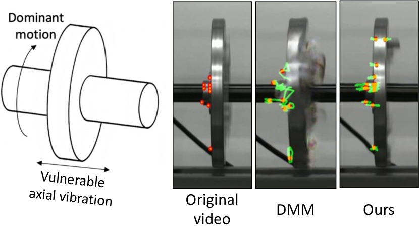
Figure 1: Importance of axial motion magnification. When identifying faults in rotating machinery, analysis of the vulnerable axial vibration is critical [21]. Existing motion magnification methods, e.g., Deep Motion Magnification (DMM) [23] amplifies motions along all axes, which yield artifacts driven by amplifying the dominant motion in this sample. It hinders the analyses of vulnerable axial vibration. This motivates the importance of our axial motion magnification that magnifies decomposed motions along a user-specified axis. We magnify the axial vibration only, achieving artifact-free magnified results and the legibility of critical motions. For the visualization purpose, we overlay the sampled trajectories obtained from the Kanade-Lucas-Tomasi (KLT) Tracker [20].

In this work, we focus on improving the legibility of magnified motion by proposing a novel concept, axial motion magnification, which magnifies decomposed motions along a user-specified direction. All the existing works, e.g.,  [40, 37, 38, 23, 16, 29], have overlooked this key importance of the legibility according to axes in practice. There are many practical cases where the importance of motion varies according to axes. For example, in the fault detection application of machines in Fig. 1, even small motions along the vulnerable axis are critical while bigger and dominant rotational motions are not [21]. Likewise, many apparatus consisting of natural or artificial materials often have vulnerable axes due to the asymmetry property of microstructures, e.g., fracture toughness [35, 3, 17]. This motivates us to separately analyze motions according to axes.

Specifically, we propose a novel learning-based axial motion magnification method, where the motions in a user-specified axis are magnified. Our method can independently magnify small motions along two orthogonal orientation axes with two independent magnification factors for each axis, which facilitates the analysis of complex small motions in the lens of axes favorable to the user. To this end, we propose Motion Separation Module (MSM) that disentangles the motion representation into two orthogonal orientations and manipulates it into the direction specified by the user. Additionally, for training the neural network, we develop and build a new synthetic dataset for the axial motion magnification task. Thereby, our proposed approach adds user control capability, while improving the legibility of resulting motions along a certain axis. We can directly adopt our method to the generic motion magnification task and achieve favorable performance against competing methods. We summarize our main contributions as follows:

• We propose the first learning-based axial motion magnification method, which allows us to selectively amplify small motions along a specific direction.

• We construct a new synthetic dataset to train the new axial motion magnification model.

• We conduct analyses and find that adopting the Motion Separation Module (MSM) is effective in distinguishing small motions from noise.

2 Related Work

Liu et al. [19] first pioneered the video motion magnification task, which involves estimating explicit motion trajectory via optical flow, known as the Lagrangian representation [40], to generate magnified frames. They group and filter the motion trajectories based on motion similarity and user’s intervention, and magnify them through explicit image warping, followed by video inpainting to fill holes created by the explicit warping.

Wu et al. [40] re-formulate the motion magnification task as an Eulerian method that represents motion by intensity changes of pixels at each fixed location without actual movement [12]. The Eulerian approach, e.g., [40, 37, 38, 41, 31, 23, 32, 33, 34], becomes standard in motion magnification due to its noise robustness, sensitivity to small motions, and simplified system by avoiding the challenges of the warp and inpaint approach for filling holes and handling occlusions. The system of the Eulerian methods typically consists of motion representation, manipulation, and reconstruction. The previous works can be categorized into two main focuses: 1) proposing motion representations or 2) motion manipulation methods.

In the first category, Wu et al. [40] present the motion representation motivated by the first-order Taylor expansion, which is implemented by Laplacian pyramid as spatial decomposition. Wadhwa et al. [37, 38] enhance the representation by modeling the motion as phase representations, which are implemented by complex steerable filters [27] in [37] and Riesz transform in [38] as spatial decomposition, respectively. These works rely on the classic signal processing theory with such hand-designed spatial filter designs, which do not model non-linear phenomenons such as occlusion or disocclusion of objects. This yields artifacts and noisy results, especially in object boundaries.

To deal with it, Oh et al. [23] first coined learning-based video motion magnification, called Deep Motion Magnification (DMM), by modeling motion representation with deep neural networks. Since no real data exists for training video motion magnification, they propose a method to build motion magnification synthetic data. With the development, other learning-based variants [16, 29] have been proposed by focusing on neural network architectures. These approaches demonstrate promising results by effectively handling diverse challenging scenarios such as occlusion and noisy inputs. Also, the motion magnification factors of the data-driven approaches can be controlled by the way the synthetic dataset is generated, while those of the traditional methods [40, 37] are theoretically restricted.

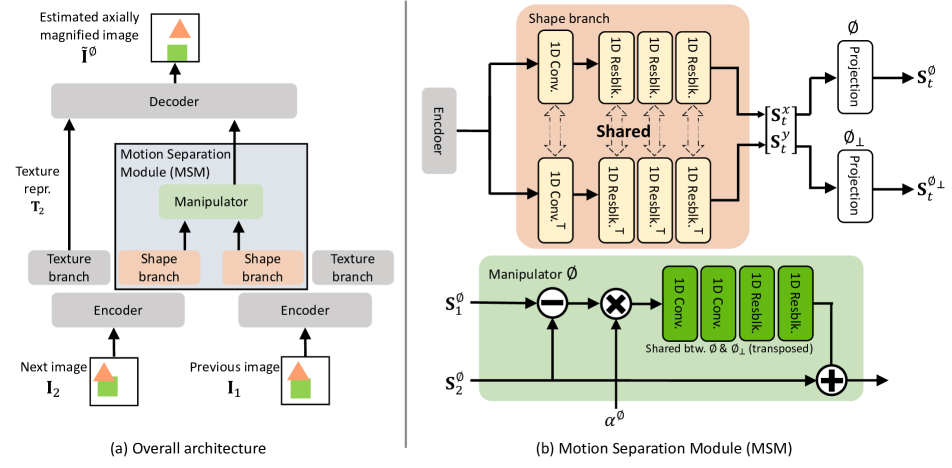
Figure 2: Proposed network architecture. (a) The Encoder outputs features from input images and the features are fed to the Texture branch and Motion Separation Module (MSM). (b) Using weight-shared 1D convolutions, the Shape branch extracts shape representations along the $x$ and $y$-axis, which are sequentially projected by the user-defined direction $\phi$ and $\phi_{\perp}$, respectively. The Decoder predicts the axially magnified image from the outputs from the Texture branch and MSM.

In the second category, when Wu et al. [40] present Eulerian motion magnification, they also propose to use a temporal filter on the motion representation to select the motion frequency of interest. This allows to suppress the noise by focusing on specific motions as well as increasing the legibility of magnified motion. There were attempts to extend to increase the legibility by proposing temporal filters to magnify different types of motions and deal with artifacts from large motions: acceleration [41, 31], intensity-aware temporal filter [34], velocity or all-frequency filter [23]. Our work is compatible with all these methods.

In this work, we present a new notion of motion magnification by disentangling motion axes of the user’s interest. We design a neural architecture to induce disentanglement of motion in oriented axes. Also, to train such a model, we propose the synthetic data generation pipeline for the axial motion magnification task. In contrast to all the existing Eulerian methods, which overlook the directional legibility of the resulting magnified motions, we add an additional feature to motion magnification.

3 Learning-based Axial Motion Magnification

In this section, we first briefly discuss preliminaries about generic motion magnification, which refers to the methods that amplify the motion regardless of motion direction, including the prior arts [40, 23, 29, 16] (Sec. 3.1). Then, we re-frame the motion magnification problem in the view of axial motion magnification (Sec. 3.2), and elaborate on our network architecture, synthetic data generation method, and objective functions (Sec. 3.3).

3.1 Preliminary – Generic Motion Magnification

Following the convention [40, 37], for simplicity, we consider the 1D image intensity being shifted by the displacement function $\delta(x,t)$ parameterized by position $x$ and time $t$. It can be generalized to local translational motion in 2D image [40]. Given an underlying intensity profile function $f(\cdot)$, the 1D image intensity $I(x,t)$ can be represented as

$$I(x,t)=f(x+\delta(x,t)).$$ (1)

The goal of motion magnification is to synthesize the magnified image intensity $\hat{I}(x,t)$:

$$\hat{I}(x,t)=f(x+(1+\alpha)\delta(x,t)),$$ (2)

where $\alpha$ denotes the magnification factor. The key factor of motion magnification methods lies in the extraction of the displacement function $\delta(x,t)$ from Eq. (1). If $\delta(x,t)$ can be decomposed, we can approximate $\hat{I}(x,t)$ by multiplying $\delta(x,t)$ with the magnification factor $\alpha$ and applying the reverse of the decomposition process. However, it is challenging and ill-posed to extract exact displacements from the observed intensity images [40]. Instead, the prior arts approximately decompose $\delta(x,t)$; for example, Wu et al. [40] use the first-order Taylor expansion:

$$I(x,t)\approx f(x)+\delta(x,t)\tfrac{\partial f(x)}{\partial x}.$$ (3)

Learning-based methods [23, 16, 29] design neural networks that have intermediate representations related to $\delta(\cdot)$, called shape representation. The representations are multiplied by $\alpha$, followed by reconstruction for magnification.

3.2 Axial Motion Magnification

To introduce the axial motion magnification task, we now consider the 2D spatial coordinate by slightly abusing the notations, e.g., $\textbf{x}=(x,y)$ to refer to the coordinate in the 2D image intensity $I(\textbf{x},t)$.

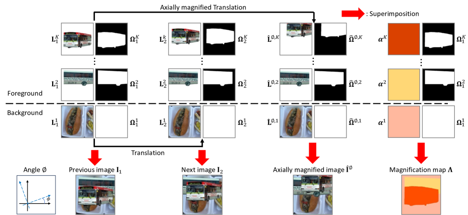
Figure 3: Synthetic data generation pipeline for axial motion magnification. From the sampled background and foregrounds, each with their own segmentation masks, we compose the previous layer images $\{{\mathbf{L}}^{k}_{1}\}_{k=1}^{K}$ and masks $\{\boldsymbol{\Omega}^{k}_{1}\}_{k=1}^{K}$. To generate next layer images $\{{\mathbf{L}}^{k}_{2}\}_{k=1}^{K}$ and masks $\{\boldsymbol{\Omega}^{k}_{2}\}_{k=1}^{K}$, we apply the random translations to $\{{\mathbf{L}}^{k}_{1}\}_{k=1}^{K}$ and $\{\boldsymbol{\Omega}^{k}_{1}\}_{k=1}^{K}$. Axially magnified layer images $\{\hat{{\mathbf{L}}}^{\phi,k}\}_{k=1}^{K}$ and masks $\{\hat{\boldsymbol{\Omega}}^{\phi,k}\}_{k=1}^{K}$ are also synthesized by translations but with the axially magnified translation parameters. The previous, next, and axially magnified layer images and masks are then superimposed into a single image to yield $\textbf{I}_{1}$, $\textbf{I}_{2}$, and $\hat{\textbf{I}}^{\phi}$, respectively. The dataset also include angles $\phi$ and the object-wise magnification maps $\boldsymbol{\Lambda}$ generated by superimposing $\{\boldsymbol{\alpha}^{k}\}_{k=1}^{K}$ with $\{\boldsymbol{\Omega}_{1}^{k}\}_{k=1}^{K}$.

Problem Definition

We can represent $I(\textbf{x},t)=f(\textbf{x}+\boldsymbol{\delta}(\textbf{x},t))$ with a 2D displacement vector $\boldsymbol{\delta}(\textbf{x},t)\in\mathbb{R}^{2}$. Given an angle $\phi\,{\in}\,\mathbb{R}$ of the user-specified direction of interest, the goal of the axial motion magnification task is to isolate and amplify the motion component corresponding to the direction angle $\phi$ within the displacement vector. We represent the axially magnified image $\hat{I}^{\phi}(\textbf{x},t)$ as

$$\hat{I}^{\phi}(\textbf{x},t)=f(\textbf{x}+\alpha^{\phi}\boldsymbol{\delta}^{\phi}(\textbf{x},t)),$$ (4)

where $\alpha^{\phi}\geq 0$ denotes the axial magnification factor and $\boldsymbol{\delta}^{\phi}(\textbf{x},t)$ represents the projection of $\boldsymbol{\delta}(\textbf{x},t)$ onto a 2D directional unit vector $\textbf{p}^{\phi}$ of the angle $\phi$, i.e., the motion component. We can break down the motion component $\boldsymbol{\delta}^{\phi}(\textbf{x},t)$ into:

$$\boldsymbol{\delta}^{\phi}(\textbf{x},t)=\operatorname{proj}_{\mathbf{\textbf{p}^{\phi}}}{\boldsymbol{\delta}(\textbf{x},t)},$$ (5)

which we refer to as angular modulation. Thus, the problem boils down to how to extract $\boldsymbol{\delta}^{\phi}$ from the input video.

3.3 Neural Networks and Training

Since the previous learning-based methods [23, 29, 16] were designed for generic motion magnification, we design a new neural network architecture and a training dataset to learn the motion representation proportional to $\boldsymbol{\delta}^{\phi}$.

Network Architecture

Our whole architecture consists of Encoder, Texture branch, Shape branch, Manipulator, and Decoder similar to DMM [23] (see Fig. 2-(a)), where texture represents color and texture-related information while shape represents scene structure-related information that later leads to motion $\boldsymbol{\delta}$ [23]. To extract axial shape representations, we design Motion Separation Module (MSM) consisting of the completely re-designed and dedicated Shape branch and Manipulator as depicted in Fig. 2-(b). In MSM, instead of extracting a single specified direction $\boldsymbol{\delta}^{\phi}$, we design to extract its orthogonal direction $\boldsymbol{\delta}^{\phi_{\perp}}$ as well.

Given consecutive input images $\textbf{I}_{t}\in\mathbb{R}^{H\times W\times 3}$ at $t=1$ and $t=2$, texture representations $\textbf{T}_{t}\in\mathbb{R}^{H/4\times W/4\times 32}$ are obtained by $\textbf{T}_{t}=F(E(\textbf{I}_{t}))$, where $E(\cdot)$ and $F(\cdot)$ denote the Encoder and the Texture branch, respectively. The outputs of $E$ are fed into MSM.

To extract he motion representations along two orthogonal orientations and manipulate them based on the user-defined angle, we grant the learnable parameters to learn the directionality in MSM. Our Shape branch $G(\cdot)$ first extracts the axial shape representations along the canonical $x$ and $y$-axes by applying weight-shared 1D convolutions but with spatially transposing the convolution kernels, yielding $[\textbf{S}^{x}_{t},\textbf{S}^{y}_{t}]$=$G(E(\textbf{I}_{t}))$ where $\textbf{S}^{x}_{t},\textbf{S}^{y}_{t}\in\mathbb{R}^{H/2\times W/2\times 32}$. Then, these are projected according to the user-defined direction $\phi$ by the Projection layer, which produces axial shape representations, i.e., $\textbf{S}^{\phi}_{t}$ and $\textbf{S}^{\phi_{\perp}}_{t}$.

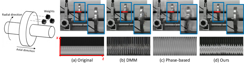
Figure 4: [Left] Imposing an imbalance on a rotor, [Right] Qualitative results in axial motion magnification scenario. We attach weights to a rotor to impose an imbalance and acquire rotor imbalance sequence, which has axial vibrations. Then, we amplify only the motion of rotor’s axial direction with the magnification factor $\alpha=40$, using ours and phase-based method [37]. We also show the magnified result of DMM [23] as one reference result of generic motion magnification methods. Our method produces magnified output frames without artifacts and exhibits the $x$-t graph showing clearly legible axial vibrations, while the magnified results of phase-based method and DMM both suffer from severe artifacts and have unclear axial vibrations in the $x$-t graph.

The Manipulator $M(\cdot)$ calculates the difference of the axial shape representations and magnifies them by multiplying the axial magnification factor $\alpha^{\phi}$. Then, these manipulated representations are fed into subsequent 1D convolutions, and added to the axial shape representation $\textbf{S}^{\phi}_{2}$. For $\phi_{\perp}$, we use the same manipulator, of which weights are shared but spatially transposed, for applying $\alpha^{\phi_{\perp}}$. Note that, with this separation of $\phi$ and $\phi_{\perp}$, we can set the magnification factors $\alpha^{\phi}$ and $\alpha^{\phi_{\perp}}$ independently, enabling broad applications of controls as another benefit. Finally, the Decoder $D(\cdot)$ predicts the axially magnified output frame $\tilde{\textbf{I}}^{\phi}$ as

$$\tilde{\textbf{I}}^{\phi}=D\left(\textbf{T}_{2},M(\textbf{S}^{\phi}_{1},\textbf{S}^{\phi}_{2},\alpha^{\phi}),M(\textbf{S}^{\phi_{\perp}}_{1},\textbf{S}^{\phi_{\perp}}_{2},\alpha^{\phi_{\perp}})\right).$$ (6)

Note that the Decoder is designed and trained to deal with both $S^{\phi}$ and $S^{\phi_{\perp}}$ in a unified manner. This enables the network to conduct both generic and axial motion magnification, given the user setting of the angle $\phi$.

Training Data Generation

In the real world, acquiring consecutive images and magnified images at the same time is impossible. Due to this, DMM [23] proposes a synthetic training dataset for the generic motion magnification task. While the dataset is effective for learning generic motion magnification, it is not effective and sufficient to induce the disentanglement of the axial property we need. Thus, we propose a new synthetic dataset specifically designed for learning the axial motion magnification, where the motion between $\textbf{I}_{1}$ and $\hat{\textbf{I}}^{\phi}$ is associated with the angle $\phi$ and axial magnification factor vector $\boldsymbol{\alpha}{=}(\alpha^{\phi};\alpha^{\phi_{\perp}})$. Motivated by the established synthetic dataset generation protocol of DMM, we synthesize the training data pairs using the widely adopted simple copy-paste method [23, 13].

Figure 3 shows the synthetic data generation pipeline. We sample one background from COCO [18] and $K{-}1$ number of foreground textures with segmentation masks from PASCAL VOC [10]. These elements are randomly located on image planes of resolution 384$\times$384 to produce $K$ previous layer images $\{{\mathbf{L}}^{k}_{1}\}_{k=1}^{K}$ and corresponding masks $\{\boldsymbol{\Omega}^{k}_{1}\}_{k=1}^{K}$. Following this, with randomly sampled $K$ translation parameters $\{\textbf{d}^{k}\}_{k=1}^{K}$, we generate the next layer images $\{{\mathbf{L}}^{k}_{2}\}_{k=1}^{K}$ and masks $\{\boldsymbol{\Omega}^{k}_{2}\}_{k=1}^{K}$ by translating the initial layers and masks according to $\{\textbf{d}^{k}\}_{k=1}^{K}$. For the axially magnified layer images $\{\hat{{\mathbf{L}}}^{\phi,k}\}_{k=1}^{K}$ and their masks $\{\hat{\boldsymbol{\Omega}}^{\phi,k}\}_{k=1}^{K}$, we sample $K$ axial magnification vectors $\{\boldsymbol{\alpha}^{k}\}_{k=1}^{K}$ and a single degree of angle $\phi$. Then, we perform the same procedure as the next layers but with the axially magnified translation parameters $\{\boldsymbol{\alpha}^{k}(\operatorname{proj}_{\mathbf{\textbf{p}^{\phi}}}{\textbf{d}^{k}};\operatorname{proj}_{\mathbf{\textbf{p}^{\phi_{\perp}}}}{\textbf{d}^{k}})\}_{k=1}^{K}$. These previous, next, and axially magnified layer images and masks are then superimposed into a single image to yield $\textbf{I}_{1}$, $\textbf{I}_{2}$, and $\hat{\textbf{I}}^{\phi}$, respectively. Our dataset also includes the angle $\phi$ and the object-wise magnification map $\boldsymbol{\Lambda}$ which is generated by superimposing $\{\boldsymbol{\alpha}^{k}\}_{k=1}^{K}$ segmented with $\{\boldsymbol{\Omega}_{1}^{k}\}_{k=1}^{K}$. We observe that $\phi$ and $\boldsymbol{\Lambda}$ are useful to learn the representations robust to the noise, which will be discussed on Sec. 4.3. We provide more details in the supplementary materials.

Loss Function

Based on the implementation of DMM [23], we apply the reconstruction, texture, and shape losses. The reconstruction loss $L_{\text{recon}}$ is $l_{1}$ loss between the ground truth of the axially magnified image $\hat{\textbf{I}}^{\phi}$ and the estimated axially magnified image $\tilde{\textbf{I}}^{\phi}$. The texture loss $L_{\text{texture}}$ and the shape loss $L_{\text{shape}}$ are $l_{1}$ losses and designed so that the texture / shape representation represents intensity / motion information, respectively. We additionally apply perceptual loss $L_{\text{per}}$ [15] and Laplacian loss $L_{\text{lap}}$ between $\hat{\textbf{I}}^{\phi}$ and $\tilde{\textbf{I}}^{\phi}$. We observed an improvement in both quantitative and qualitative results when applying these two losses together. The total loss $L_{\text{total}}$ is as follows:

$$L_{\text{total}} =L_{\text{recon}}(\hat{\textbf{I}}^{\phi},\tilde{\textbf{I}}^{\phi})+\gamma L_{\text{lap}}(\hat{\textbf{I}}^{\phi},\tilde{\textbf{I}}^{\phi})+\beta\Bigl{(}L_{\text{texture}}(\textbf{T}_{1},\textbf{T}_{2})$$

$${\,+}L_{\text{shape}}(\textbf{S}^{x}_{2},\acute{\textbf{S}}^{x}_{2}){\,+}L_{\text{shape}}(\textbf{S}^{y}_{2},\acute{\textbf{S}}^{y}_{2}){\,+}L_{\text{per}}(\hat{\textbf{I}}^{\phi},\tilde{\textbf{I}}^{\phi})\Bigr{)},$$ (7)

where $\acute{\textbf{S}}^{x}_{2}$ and $\acute{\textbf{S}}^{y}_{2}$ denote the shape representations of color perturbed next image $\acute{\textbf{I}}_{2}$ as suggested by Oh et al. [23]. We set $\beta{=}0.1$ and $\gamma{=}0.5$. Refer to the ablation study and the details of the loss functions in the supplementary material.

4 Experiments

We examine the performance of our method in comparison to other motion magnification methods, considering both cases of axial and generic motion magnification. We train our learning-based axial motion magnification network on the newly proposed dataset, which contains a total of 100k samples, for 50 epochs with a batch size of $8$ and a learning rate $2\times 10^{-4}$. We use both the dynamic and static modes in the experiments following DMM [23], without a temporal bandpass filter that separates the motion with the frequency of interest. Details and additional experiments can be found in the supplementary material, including the magnified results with the temporal bandpass filters.

4.1 Axial Motion Magnification

We evaluate our method compared to the phase-based method [37] in the axial motion magnification scenario, to demonstrate the effectiveness of the learning-based axial motion magnification. In our experiment, we modulate the phase-based to operate in axial scenario by employing a half-octave bandwidth pyramid and two orientations, with one of them having its phase representation manipulated along the axis of interest.

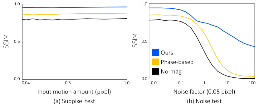
Figure 5: Quantitative results in axial motion magnification scenario. (a) In the subpixel test, our method demonstrates superior performance on SSIM over the phase-based method [37] across all input motion amount, ranging from $0.04$ to $1.0$. (b) In the noise tests when the input motion amount is 0.05 pixel, we observe a growing disparity in SSIM scores between our method and the phase-based approach, as the noise factor rises.

Qualitative Results

We will demonstrate the advantage of our method that it can amplify only the motion along the axis of interest while disentangling the motions in uninterested directions that interfere with motion analysis. To illustrate this concept concretely, consider a scenario where a shaft is rotating in the radial direction. In such cases, magnifying and examining the motion along the axial direction, which is crucial to assess the condition of the rotating machinery [21], becomes challenging due to the dominance of rotational motion over the axial component. We conduct an experiment as depicted in Fig. 4 to illustrate this challenge, by attaching weights to a rotor to impose an imbalance, which results in axial vibrations. Then, we acquire a video of the imbalanced rotor, called rotor imbalance sequence, using a camera that captures $120$ Frames Per Second (FPS). We choose a horizontal-axis line in the original frame and plot $x$-t graphs for the magnified output frames from each method, respectively. Note that we also provide the result of Deep Motion Magnification (DMM) [23] as a reference to compare the results of axial motion magnification with generic motion magnification.

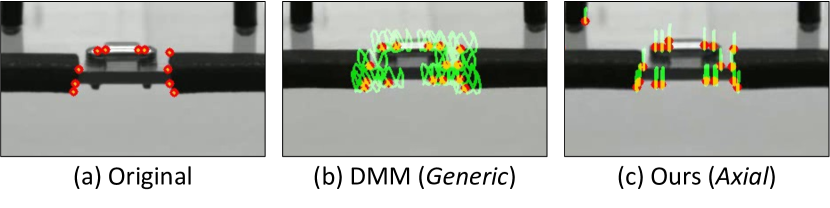
Figure 6: Motion legibility improvement. We visualize the 40$\times$ magnified frames of the structure, which are overlaid with the sampled trajectories from the KLT tracker. Ours shows simplified and legible motion trajectories when magnifying along the specific axis (i.e., y-axis in this case), while DMM [23] produces the trajectories that are more complex and challenging to interpret.

As shown in Fig. 4, our method produces the magnified output frames without artifacts and exhibits the $x$-t graph that clearly depicts axial vibrations. In contrast, the phase-based method [37] suffers from severe ringing artifacts, likely due to the overcompleteness of the complex steerable filter [28, 27], which cannot perfectly separate the phase representation into two orthogonal directions. DMM yields the magnified frames with artifacts and unclear axial vibrations in the $x$-t graph, since the representation of generic motion magnification method struggles to disentangle the dominant motion of the radial direction from the motion of interest, i.e., axial direction’s motion.

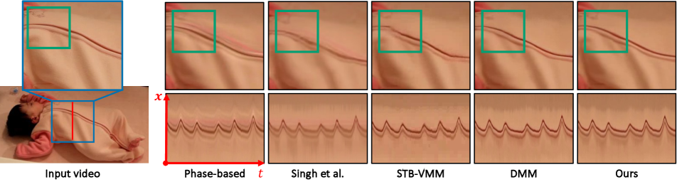
Figure 7: Qualitative results in generic motion magnification scenario. We amplify the motions in baby sequence with the magnification factor $\alpha=20$, using phase-based method [37], Singh et al. [29], STB-VMM [16], DMM [23], and our method. Both Ours and DMM favorably preserve the edges of the baby’s clothing and show no ringing artifacts in the magnified output frames and the $x$-t graphs. In contrast, the magnified output frames of the phase-based, STB-VMM, and Singh et al. show severe ringing artifacts or blurry results.

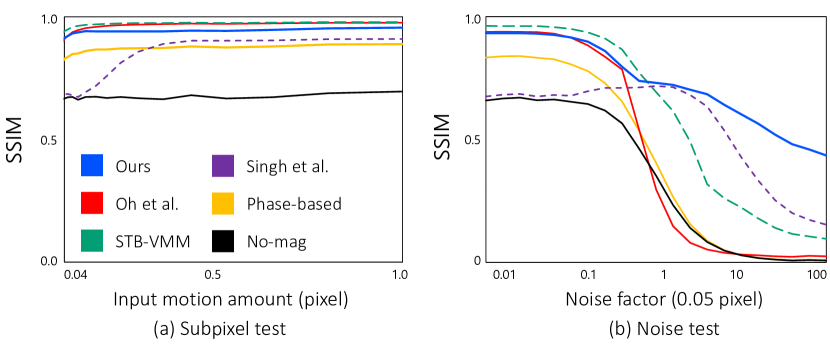
Figure 8: Quantitative results in generic motion magnification scenario. (a) In the subpixel test, which measures performance with varying input motion amount, Ours outperforms phase-based method [37] and Singh et al. [29], and achieves favorable performance on SSIM compared to DMM [23] and STB-VMM [16]. (b) In the noise tests, compared to other methods, ours shows outstanding noise tolerance as the noise factor increases.

Quantitative Results

To quantitatively evaluate our learning-based axial motion magnification method, we generate axial evaluation dataset based on the validation dataset of DMM [23]. The method of generating the dataset is almost the same as that of the training dataset. One difference is that we adjust the motion amplification factor to ensure that the amplified motion magnitude along a random axis is equal to 10. The motion amplification factor for the other axis is set to half the value. Note that we set $\phi$ to be $0$ for this quantitative evaluation. We report the Structural Similarity Index (SSIM) [39] between the ground truth and output frames of the phase-based method and ours. As a reference, we provide the SSIM between ground truth and input frames. Figure 5 summarizes the results. We measure the SSIM by varying the levels of motion (Fig. 5-(a) Subpixel test) and additive noise (Fig. 5-(b) Noise test) in the input images. The number of evaluation data samples for each level of motion and noise is $1,000$. Regardless of the input motion magnitude and noise level, our method consistently outperforms the phase-based approach, which indicates that our proposed network architecture and dataset are effective for learning axis-wise disentangled representations.

Motion Legibility Comparison

To demonstrate the efficacy of our method in improving the legibility of magnified motions, we use a structure that exhibits complex movements. We then visualize and compare the motion trajectories, tracked by the KLT tracker, of the $40\times$ magnified video sequences of this structure using both the generic method (DMM) [23] and the axial method (Ours). As shown in Fig. 6, our method shows simplified and legible trajectories when magnifying along the specific axis (i.e., $y$-axis in this case), while DMM shows the trajectories difficult to decipher the motion of the structure.

4.2 Generic Motion Magnification

While our method focuses on the axial motion magnification task, it can be readily adapted for generic motion magnification scenario. This adaptability is achieved by simply multiplying the same magnification factors with the axis-wise shape representations. In the context of generic motion magnification, to demonstrate the effectiveness of our method, we compare it with the phase-based method [37] and the learning-based methods [23, 16, 29].

Qualitative Results

We visualize the magnified output frames and plot the $x$-t graphs for the baby sequence, comparing ours with the several motion magnification methods in the generic motion magnification scenario (see Fig. LABEL:figure:generic_qualitative). Both our method and DMM [23] favorably preserve the edges of the baby’s clothing and show no ringing artifacts in the magnified results of breathing motion. In contrast, the phase-based method [37], STB-VMM [16], and Singh et al. [29] show severe ringing artifacts or blurry results.

Quantitative Results

To quantitatively verify the ability of our method in generic motion magnification, we synthesize the generic validation dataset. Unlike the axial motion magnification case, we set the motion magnification factor $\alpha$ to be identical along the $x$ and $y$ axes. We report SSIM [39] between ground truth frames and output frames from the phase-based method [37] and the learning-based methods [23, 29, 16]. As shown in Fig. 8, when the amount of input motion ranges from $0.04$ to $1.0$, ours outperforms the phase-based method and Singh et al. [29], achieving favorable performance in SSIM compared to DMM [23] and STB-VMM [16]. Our method also shows notable noise tolerance as the noise factor rises in the noise test at $0.05$ pixel.

4.3 Ablation Study

In this section, we conduct ablation studies to evaluate the impact of the Motion Separation Module (MSM) and the components of the proposed synthetic training data. For the ablation studies, we carry out quantitative experiments on the evaluation dataset of both the generic case and the axial case that has random angles.

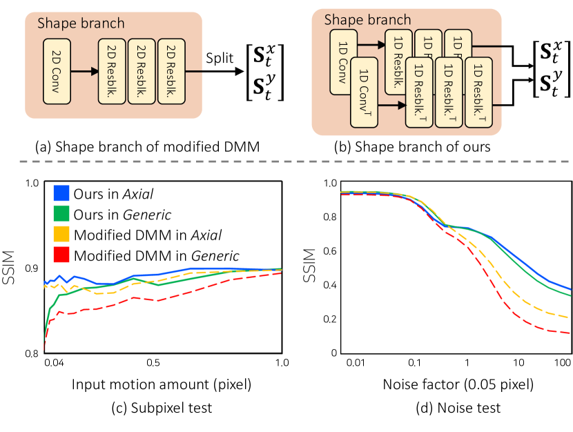
Figure 9: [Top] Architectural difference on the shape branch, [Bottom] Quantitative results of ablating Motion Separation Module (MSM). The modified DMM, desinged for ablation study, employs 2D convolutions and splits features along channel dimensions for axial motion magnification. Ours with Motion Separation Module (MSM) achieves higher SSIM in both the subpixel and noise tests on generic and axial evaluation datasets, respectively.

Motion Separation Module

To validate the effectiveness of our proposed Motion Separation Module (MSM), we design a competitor called modified DMM. While the design of the modified DMM closely resembles that of DMM [23], it differs in its approach to splitting the shape representation axis-wise for axial motion magnification. As shown in the top of Fig. 9, different from our method that uses 1D convolutions, the modified DMM employs 2D convolutions in the Shape branch and the Manipulator. The axis-wise shape representations of modified DMM are acquired by dividing the feature map along the channel dimension. We train the networks with the loss used in DMM [23] for an independent ablation on the network itself.

The bottom of Fig. 9 summarizes the quantitative results of our method and modified DMM. Ours with the MSM achieves higher SSIM on the subpixel and noise tests, compared to the modified DMM in both the axial and generic cases. These results show the effectiveness of the MSM in capturing small motions and handling noisy input images.

Components of Synthetic Training Data

To evaluate the impact of the angle $\phi$ and the object-wise motion magnification map $\boldsymbol{{\Lambda}}$, we generate the different types of training data varying the presence of these components. Our newly proposed dataset includes both $\phi$ and $\boldsymbol{{\Lambda}}$, whereas the dataset under the same configuration as DMM [23] lacks both. We further produce two additional datasets by individually adding each component to the dataset without $\phi$ and $\boldsymbol{{\Lambda}}$. Note that evaluating on the axial evaluation dataset is infeasible since it requires $\phi$ in the training time. As shown in Fig. 10, adding $\phi$ achieves no performance improvement in the subpixel test, making the network vulnerable to the noise of input images. In contrast, adding $\boldsymbol{{\Lambda}}$ leads to an increase on SSIM [39] in the subpixel test and huge robustness against noises in the noise test. The combined use of both $\phi$ and $\boldsymbol{{\Lambda}}$ yields the most significant performance improvement in the noise test, demonstrating that our proposed dataset is beneficial in the generic motion magnification task, as well.

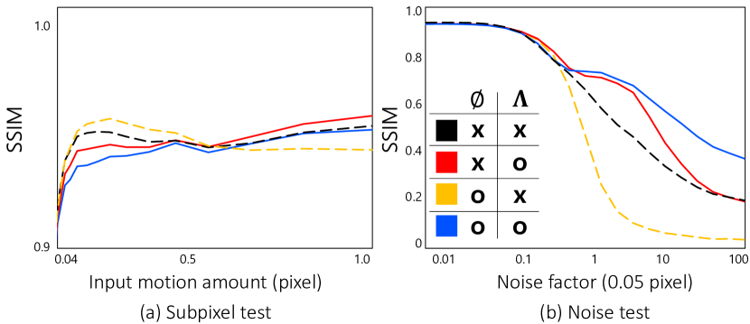
Figure 10: Ablation study of the components in data generation pipeline in the generic evaluation dataset. We generate the different types of training data varying the presence of the angle $\phi$ and the object-wise motion magnification map $\boldsymbol{{\Lambda}}$, evaluating the networks trained on each dataset configuration using the generic evaluation dataset. Using both $\phi$ and $\boldsymbol{{\Lambda}}$ demonstrates superior noise tolerance compared to the other configurations.

5 Conclusion

In this work, we present a novel concept, axial motion magnification, which improves the legibility of the motions by disentangling and magnifying the motion representations along axes specified by users. Axial motion magnification can offer easily decipherable motion information in various applications, where recognizing movements along particular axes is crucial. To this end, we propose an innovative learning-based approach for axial motion magnification, incorporating the Motion Separation Module (MSM) to effectively extract and magnify motion representations along two orthogonal orientations. To support this, we establish a new synthetic dataset generation pipeline tailored for axial motion magnification. Our proposed method provides user controllability and significantly enhances the legibility of the motions along chosen axes, showing favorable performance compared to competing methods, even in cases of generic motion magnification.

Supplementary Material

Contents

A    Implementation Details
  A.1    Data Generation
  A.2    Loss Function
B    Additional Experiments
  B.1    Physical Accuracy
  B.2    Motion Separation Effect of the MSM
  B.3    Angular Analysis of Axial Motion Magnification
  B.4    Compatibility with the Temporal Filter
  B.5    Ablation Studies of Loss Function
C    Discussion
 

Supplementary Material

In this supplementary material, we present the implementation details and additional experiments. We conclude our paper with a discussion section.

Appendix A Implementation Details

We provide the details of data generation pipeline (Sec. A.1) and the loss function for the learning-based axial motion magnification (Sec. A.2).

A.1 Data generation

Training Dataset

We randomly sample foreground textures ranging from $7$ to $14$ with segmentation masks from PASCAL VOC [10] and one background from COCO [18]. For each layer, we sample the axial magnification factor $\boldsymbol{\alpha}=(\alpha^{\phi};\alpha^{\phi_{\perp}})$ from the uniform distributions whose values are ranging from $1$ to $80$. Each element of translation parameter $\textbf{d}\in\mathbb{R}^{2}$ is uniformly sampled from the range $-u$ to $u$, where $u$ equals $\mbox{min}(10,30/\mbox{max}(\alpha^{\phi},\alpha^{\phi_{\perp}}))$. It constrains the input motion to be less than $10$ pixels or amplified motions under $30$ pixels. We sample the angle $\phi$ within the range of $0$ to $90$ degrees. Note that our method enables axial motion magnification not only in the angle $\phi$ but also in the angle $\phi_{\perp}$, making axial motion magnification possible in $0$ to $180$ degrees. To address the loss of subpixel motion due to image quantization, as proposed in DMM [23], we apply uniform quantization noise to the images before quantizing them.

Generic Evaluation Dataset

Based on the validation dataset of DMM [23], we construct the generic evaluation dataset comprising the previous image, next image, magnified image, and a single magnification factor. The generic evaluation dataset consists of two datasets for the subpixel test and noise test. The dataset for the subpixel test includes $15$ levels of motion, ranging from a motion magnitude of $0.04$ to $1.0$ pixel, changing in a logarithmic scale. The motion magnification factor is adjusted to ensure that the amplified motion magnitude becomes $10$ pixel. The dataset for the noise test includes $21$ levels of noise, ranging from a noise factor of $0.01$ to $100$ in a logarithmic scale. The amount of input motion is $0.05$ pixel, and the motion amplification factor is also set to ensure that the amplified motion magnitude becomes $10$ pixel.

Axial Evaluation Dataset

The axial evaluation dataset consists of the previous image, next image, axially magnified image, axial magnification factor vector, and angle. The axial magnification factor vector is composed of two magnification factors corresponding to two orthogonal orientations. The axial evaluation dataset also includes two datasets for the subpixel test and noise test. For the subpixel test dataset, we generate data with 15 levels of motion ranging from $0.04$ to $1.0$ pixel in a logarithmic scale. We set the motion amplification factor vector to guarantee that the magnified motion magnitude along a random orientation equals 10 pixel. For the other orientation axis, we allocate half of that value. For the noise test dataset, we have $21$ levels of noise factor ranging from $0.01$ to $100$ in a logarithmic scale. The input motion size along two orthogonal orientations is 0.05 pixel, and the motion magnification factor is set to achieve an amplified motion size of $10$ pixel for one of the orthogonal axes, while the motion magnification factor for the other axis is set to half of that value. The angle $\phi$ is randomly sampled between $0$ and $90$ degrees, except in the experiment of Fig.5 in the main paper, where $\phi$ is set to the $0$ degrees for comparison with the phase-based method [37].

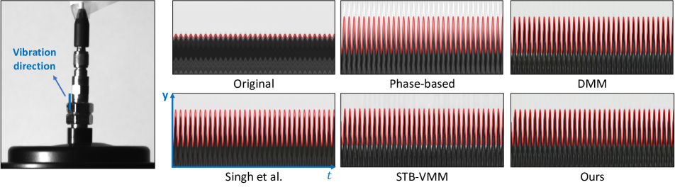
Figure 11: Physical accuracy of our method. We compare the physically calculated sinusoidal wave of pixel displacement (red line) to the $y$-t graph’s waves of $10\times$ magnified videos from motion magnification methods. We also provide the $y$-t graph’s wave of the original video and sinusoidal wave before amplification. The $y$-t graph’s wave of Ours matches the actual pixel displacement. The phase-based method [37] exhibits results consistent with the red wave of pixel displacement, albeit suffering from ringing artifacts. Other learning-based methods, such as DMM [23], STM-VMM [16], and Singh et al. [29], also demonstrate correspondences, with a marginal difference in amplification.

A.2 Loss Function

DMM [23] propose the texture loss $L_{\text{texture}}$ and shape loss $L_{\text{shape}}$ to represent intensity and motion information, respectively. These losses are combined with the reconstruction loss $L_{\text{recon}}$, resulting in the loss of DMM $L_{\text{DMM}}$. $L_{\text{DMM}}$ in the case of axial motion magnification is as follows:

$$L_{\text{DMM}} =L_{\text{recon}}(\hat{{\mathbf{I}}}^{\phi},\tilde{{\mathbf{I}}}^{\phi})+L_{\text{texture}}(\textbf{T}_{1},\textbf{T}_{2})$$

$$+L_{\text{shape}}(\textbf{S}^{x}_{2},\acute{\textbf{S}}^{x}_{2})+L_{\text{shape}}(\textbf{S}^{y}_{2},\acute{\textbf{S}}^{y}_{2}).$$ (8)

Based on the $L_{\text{DMM}}$, we also integrate perceptual loss $L_{\text{per}}$ [15] and Laplacian loss $L_{\text{lap}}$ into our total loss $L_{\text{total}}$, which corresponds to:

$$L_{\text{total}} =L_{\text{recon}}(\hat{\textbf{I}}^{\phi},\tilde{\textbf{I}}^{\phi})+\gamma L_{\text{lap}}(\hat{\textbf{I}}^{\phi},\tilde{\textbf{I}}^{\phi})+\beta\Bigl{(}L_{\text{texture}}(\textbf{T}_{1},\textbf{T}_{2})$$

$${\,+}L_{\text{shape}}(\textbf{S}^{x}_{2},\acute{\textbf{S}}^{x}_{2}){\,+}L_{\text{shape}}(\textbf{S}^{y}_{2},\acute{\textbf{S}}^{y}_{2}){\,+}L_{\text{per}}(\hat{\textbf{I}}^{\phi},\tilde{\textbf{I}}^{\phi})\Bigr{)},$$ (9)

where we set $\beta$ and $\gamma$ to 0.1 and 0.5, respectively. We train our model using two NVIDIA Titan RTX GPUs. The efficacy of $L_{\text{per}}$ and $L_{\text{lap}}$ will be discussed in the Sec. B.5.

Appendix B Additional Experiments

In this section, we assess the physical accuracy (Sec. B.1), motion separation effect of the MSM (Sec. B.2), and the behavior of our method across varying degrees (Sec. B.3). We also demonstrate the compatibility of our method with the temporal filter (Sec. B.4) and conduct ablation studies on the loss function (Sec. B.5).

B.1 Physical Accuracy

To assess the physical accuracy, we examine whether the vibrations of the magnified video, using the proposed method, matched those of actual vibrations. First, we generate a $20$Hz sinusoidal vibration using a vibration generator. Next, we obtain the peak amplitude of acceleration ($\text{m}/\text{s}^{2}$) from the attached accelerometer and convert it into a sinusoidal wave of displacement (m), which is transformed into a sinusoidal wave of pixel displacement (px) on the image plane through pinhole camera geometry. We investigate if this wave corresponds to the vibration of the $10\times$ magnified video using the static mode. The transformation from the peak amplitude of acceleration $a$ to the peak amplitude of displacement $\mu$ is as follows:

$$\mu=a/\omega^{2},$$ (10)

where the $\omega$ denotes the frequency of sinusoidal vibration. Using $\mu$, we obtain the sinusoidal wave of real-world displacement $s(t)$ over time $t$ and transform it into pixel displacement $k(t)$, which corresponds to

$$k(t)=\frac{f}{Lv}s(t).$$ (11)

The $f$, $L$, and $v$ refer to the focal length, camera-to-vibrator distance, and per-pixel sensor size.

Hyperparameters	Unit	Value
Vibration frequency $\omega$	Hz	20
Peak amplitude of acceleration $a$	$\text{m/s}^{2}$	4.11
Camera-to-vibrator distance $L$	m	2
Focal length $f$	mm	100
Per-pixel sensor size $v$	$\mu$m	5.86

Table 1: Hyperparameters for acquiring pixel displacement.

As shown in Fig. 11, the $y$-t graph’s wave of our method demonstrates a correspondence with the red wave of pixel displacement that is $10\times$ amplified. The phase-based method [37] and other learning-based methods [23, 29, 16] also show correspondences, albeit with marginal differences in amplification. These results validate the physical accuracy of our method, as well as that of other motion amplification methods. We list the hyperparameters for converting the acceleration ($\text{m}/\text{s}^{2}$) to pixel displacement (px) in Table 1.

B.2 Motion Separation Effect of the MSM

We assess the effectiveness of the Motion Separation Module (MSM) in distinguishing between two orthogonal directional motions. To explore this, we rotate the video of a vibrator oscillating solely along the $y$-axis by the angle $\phi$ and apply the $10\times$ axial motion magnification to the video along the $\phi_{\perp}$ direction using both our method and the modified DMM with the static mode. Subsequently, we compare the time slices in the direction of $\phi_{\perp}$, i.e., the direction with no motion. In this experiment, we set $\phi$ to $30$ degrees. Figure 12 demonstrates the results. Unlike the $\phi_{\perp}$-t graph of the original, where there is no motion in the $\phi_{\perp}$ direction, modified DMM fails to separate the motion and exhibits motion in the $\phi_{\perp}$ direction. In contrast, Ours with MSM effectively separates the motions in two orthogonal directions, showing results similar to the original in the $\phi_{\perp}$ direction.

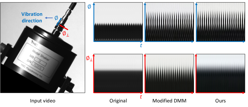
Figure 12: Motion separation experiment with MSM. Along the $\phi_{\perp}$ direction, we apply the $10\times$ axial motion magnification to the video of a vibrator oscillating only in the $\phi$ direction using Ours and the modified DMM. Unlike the $\phi_{\perp}$-t graph of the original, the modified DMM exhibits vibration in the $\phi_{\perp}$ direction due to the unsuccessful motion separation. In contrast, our method, which uses MSM, effectively separates two orthogonal motions and presents a $\phi_{\perp}$-t graph similar to that of the original.

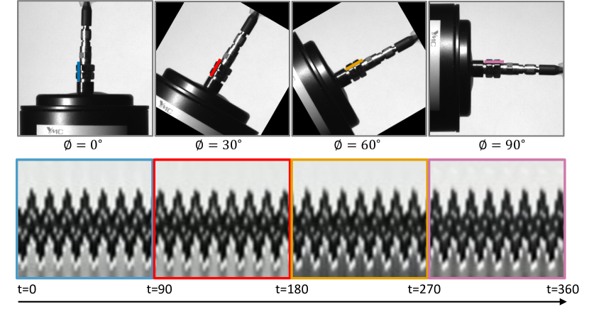
Figure 13: Axial motion magnification results across various angles. We applied axial motion magnification to amplify motion in the direction $\phi$ for vibrator videos rotated at various angles $\phi$. The time slices of axially amplified videos using our method show the smooth transition at boundaries where the angle $\phi$ changes.

B.3 Angular Analysis of Axial Motion Magnification

Our learning-based axial motion magnification can magnify the motion along the user-defined direction. We examine whether the behavior of our learning-based axial motion magnification remains consistent with changing angles. As shown in Fig. 13, we rotate the vibrator video at various angles $\phi$ and apply $10\times$ axial motion magnification to amplify only the motion corresponding to $\phi$. Subsequently, time slices are obtained from the rotated videos for the same point, and these slices are connected over time. The connected time slices exhibit a smooth transition at boundaries where the angle $\phi$ changes. This demonstrates the consistent behavior of our learning-based axial motion magnification across various angles.

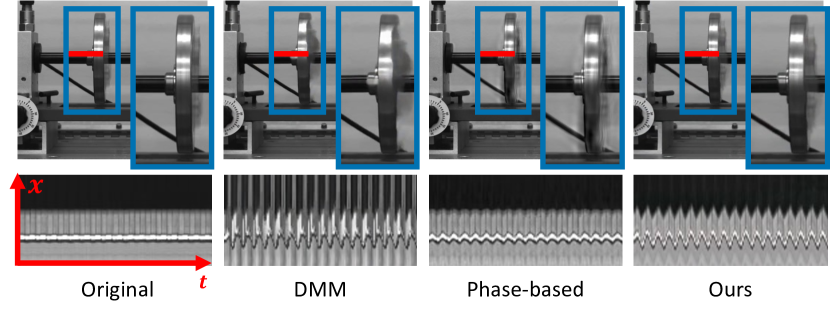
Figure 14: Axial motion magnification with temporal filter. With the Butterworth filter, we $40\times$ magnify the rotor imbalance sequence along the $x$-axis, i.e., the axial direction, using Ours and phase-based method [37]. We also show the $40\times$ magnified result of DMM [23] with the temporal filter as one reference result of generic motion magnification methods. Our shows the clear magnified output frame and $x$-t graph, which represents legible axial vibrations. The magnified frame of the phase-based method suffers from ringing artifacts, and the DMM demonstrates the magnified frames with artifacts and unclear axial vibrations due to dominant rotational motion, even with the temporal filter.

B.4 Compatibility with the Temporal Filter

Our learning-based axial motion magnification is compatible with temporal filters. To demonstrate compatibility with a temporal filter during axial motion magnification, we apply a $40\times$ magnification to the rotor imbalance sequence along the $axial$ direction ($x$-axis) using Ours and phase-based method [37]. We use a Butterworth filter with a frequency range of $3\sim 20$Hz as the temporal filter. The result obtained from DMM [23] with the same filter is provided for comparison with generic motion magnification. As shown in Fig. 14, the magnified frame using our method is free from artifacts, and the $x$-t graph clearly depicts axial vibrations. In contrast, the output of the phase-based method exhibits ringing artifacts, and DMM produces magnified frames with artifacts and unclear axial vibrations due to dominant rotational motion, even with the temporal filter.

In the case of generic motion magnification, our method is also compatible with the temporal filter, as illustrated in Fig. 15. When magnifying the baby sequence 20 times with the IIR filter with a range of $0.04\sim 0.4$Hz, Ours and DMM preserve the boundaries of the baby’s clothing and clearly represent the breathing motion of the baby. The phase-based approach also represents the breathing motion well, but it exhibits slight ringing artifacts.

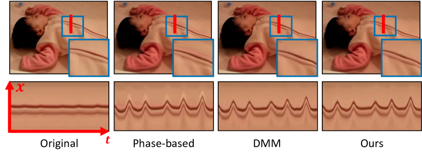
Figure 15: Generic motion magnification with temporal filter. We applied generic motion magnification to the baby sequence using the phase-based, DMM, and our methods. The motion magnification factor is set to $20$, and we use the IIR filter as the temporal filter. Ours and DMM preserve the boundaries of the baby’s cloth and depict the breathing motion well. The phase-based method exhibits slight ringing artifacts.

B.5 Ablation Studies of Loss Function

We analyze the effects of $L_{\text{per}}$ and $L_{\text{lap}}$ quantitatively and qualitatively. We progressively introduce $L_{\text{per}}$ and $L_{\text{lap}}$ to $L_{\text{DMM}}$ and evaluate the performance of the networks trained with these additional losses.

Quantitative Analysis

To quantitatively assess the effects of additional losses, we evaluate the performance on both generic and axial evaluation datasets. Figure 16 demonstrates the results. Applying both $L_{\text{per}}$ and $L_{\text{lap}}$ shows superior performance in subpixel and noise tests on both axial and generic evaluation datasets. Adding $L_{\text{per}}$ achieves marginal performance improvement in the two subpixel tests, but the robustness against noises in the generic evaluation dataset decreases. This result is consistent with the observation of DMM [23] that perceptual loss do not yield a noticeable difference. Similarly, using $L_{\text{lap}}$ alone exhibits the trade-offs similar to $L_{\text{per}}$.

Qualitative analysis

We observe that applying both $L_{\text{per}}$ and $L_{\text{lap}}$ is effective to represent the motion of rigid objects. We apply the $40\times$ axial motion magnification along the $y$-axis to the rotor imbalance sequence. As shown in Fig. 17, applying both $L_{\text{per}}$ and $L_{\text{lap}}$ preserves the boundary of the shaft well. However, in other cases, the boundary of the shaft is distorted.

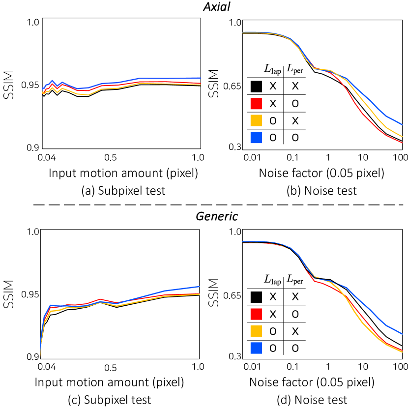
Figure 16: Quantitative results on different combinations of losses. Applying both $L_{\text{per}}$ and $L_{\text{lap}}$ shows superior performance in subpixel and noise tests on both axial and generic evaluation datasets. In contrast, applying either $L_{\text{per}}$ or $L_{\text{lap}}$ alone demonstrates a trade-off compared to applying none.

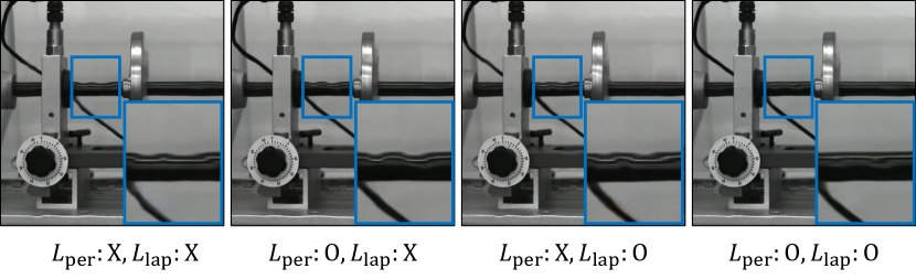
Figure 17: Qualitative results on different combinations of losses. When the rotor imbalance sequence is axially magnified $40$ times along the $y$-axis, applying both $L_{\text{per}}$ and $L_{\text{lap}}$ effectively preserves the boundary of the shaft.

Appendix C Discussion

To improve the legibility of magnified motion, we propose a novel concept, axial motion magnification. Additionally, we propose a new learning-based axial motion magnification method, incorporating a training dataset. Although axial motion magnification serves as one branch that enhances user convenience, another branch can be the method to perform motion magnification in real-time, which is useful and beneficial for various applications of motion magnification. Our method operates at 15.6 FPS on 720p videos, and DMM operates at 18.1 FPS, which does not achieve real-time performance. Improving the efficiency of learning-based axial motion magnification requires further research.

References

- Balakrishnan et al. [2013] Guha Balakrishnan, Fredo Durand, and John Guttag. Detecting pulse from head motions in video. In Proceedings of the IEEE conference on computer vision and pattern recognition, pages 3430–3437, 2013.
- Brattoli et al. [2021] Biagio Brattoli, Uta Büchler, Michael Dorkenwald, Philipp Reiser, Linard Filli, Fritjof Helmchen, Anna-Sophia Wahl, and Björn Ommer. Unsupervised behaviour analysis and magnification (ubam) using deep learning. Nature Machine Intelligence, 3(6):495–506, 2021.
- Brodnik et al. [2021] NR Brodnik, Stella Brach, CM Long, G Ravichandran, B Bourdin, KT Faber, and K Bhattacharya. Fracture diodes: Directional asymmetry of fracture toughness. Physical Review Letters, 126(2):025503, 2021.
- Cha et al. [2017] Y-J Cha, Justin G Chen, and Oral Büyüköztürk. Output-only computer vision based damage detection using phase-based optical flow and unscented kalman filters. Engineering Structures, 132:300–313, 2017.
- Chen et al. [2014] Justin G Chen, Neal Wadhwa, Young-Jin Cha, Frédo Durand, William T Freeman, and Oral Buyukozturk. Structural modal identification through high speed camera video: Motion magnification. In Topics in Modal Analysis I, Volume 7: Proceedings of the 32nd IMAC, A Conference and Exposition on Structural Dynamics, 2014, pages 191–197. Springer, 2014.
- Chen et al. [2015a] Justin G Chen, Neal Wadhwa, Young-Jin Cha, Frédo Durand, William T Freeman, and Oral Buyukozturk. Modal identification of simple structures with high-speed video using motion magnification. Journal of Sound and Vibration, 345:58–71, 2015a.
- Chen et al. [2015b] Justin G Chen, Neal Wadhwa, Frédo Durand, William T Freeman, and Oral Buyukozturk. Developments with motion magnification for structural modal identification through camera video. In Dynamics of Civil Structures, Volume 2, pages 49–57. Springer, 2015b.
- Chen et al. [2017] Justin G Chen, Abe Davis, Neal Wadhwa, Frédo Durand, William T Freeman, and Oral Büyüköztürk. Video camera–based vibration measurement for civil infrastructure applications. Journal of Infrastructure Systems, 23(3):B4016013, 2017.
- Davis et al. [2014] Abe Davis, Michael Rubinstein, Neal Wadhwa, Gautham J Mysore, Fredo Durand, and William T Freeman. The visual microphone: Passive recovery of sound from video. 2014.
- Everingham et al. [2010] Mark Everingham, Luc Van Gool, Christopher KI Williams, John Winn, and Andrew Zisserman. The pascal visual object classes (voc) challenge. International journal of computer vision, 88(2):303–338, 2010.
- Fan et al. [2021] Wenkang Fan, Zhuohui Zheng, Wankang Zeng, Yinran Chen, Hui-Qing Zeng, Hong Shi, and Xiongbiao Luo. Robotically surgical vessel localization using robust hybrid video motion magnification. IEEE Robotics and Automation Letters, 6(2):1567–1573, 2021.
- Freeman et al. [1991] William T Freeman, Edward H Adelson, and David J Heeger. Motion without movement. ACM SIGGRAPH, 25(4):27–30, 1991.
- Ghiasi et al. [2021] Golnaz Ghiasi, Yin Cui, Aravind Srinivas, Rui Qian, Tsung-Yi Lin, Ekin D Cubuk, Quoc V Le, and Barret Zoph. Simple copy-paste is a strong data augmentation method for instance segmentation. In Proceedings of the IEEE/CVF conference on computer vision and pattern recognition, pages 2918–2928, 2021.
- Janatka et al. [2020] Mirek Janatka, Hani J Marcus, Neil L Dorward, and Danail Stoyanov. Surgical video motion magnification with suppression of instrument artefacts. In Medical Image Computing and Computer Assisted Intervention–MICCAI 2020: 23rd International Conference, Lima, Peru, October 4–8, 2020, Proceedings, Part III 23, pages 353–363. Springer, 2020.
- Johnson et al. [2016] Justin Johnson, Alexandre Alahi, and Li Fei-Fei. Perceptual losses for real-time style transfer and super-resolution. In Computer Vision–ECCV 2016: 14th European Conference, Amsterdam, The Netherlands, October 11-14, 2016, Proceedings, Part II 14, pages 694–711. Springer, 2016.
- Lado-Roigé and Pérez [2023] Ricard Lado-Roigé and Marco A Pérez. Stb-vmm: Swin transformer based video motion magnification. Knowledge-Based Systems, 269:110493, 2023.
- Li et al. [2023] Beichen Li, Bolei Deng, Wan Shou, Tae-Hyun Oh, Yuanming Hu, Yiyue Luo, Liang Shi, and Wojciech Matusik. Computational discovery of microstructured composites with optimal strength-toughness trade-offs. arXiv preprint arXiv:2302.01078, 2023.
- Lin et al. [2014] Tsung-Yi Lin, Michael Maire, Serge Belongie, James Hays, Pietro Perona, Deva Ramanan, Piotr Dollár, and C Lawrence Zitnick. Microsoft coco: Common objects in context. In European Conference on Computer Vision (ECCV), 2014.
- Liu et al. [2005] Ce Liu, Antonio Torralba, William T Freeman, Frédo Durand, and Edward H Adelson. Motion magnification. ACM transactions on graphics (TOG), 24(3):519–526, 2005.
- Lucas and Kanade [1981] Bruce D Lucas and Takeo Kanade. An iterative image registration technique with an application to stereo vision. In IJCAI’81: 7th international joint conference on Artificial intelligence, pages 674–679, 1981.
- Luo et al. [2021] Yin Luo, Wenqi Zhang, Yakun Fan, Yuejiang Han, Weimin Li, and Emmanuel Acheaw. Analysis of vibration characteristics of centrifugal pump mechanical seal under wear and damage degree. Shock and Vibration, 2021:1–9, 2021.
- Moya-Albor et al. [2020] Ernesto Moya-Albor, Jorge Brieva, Hiram Ponce, and Lourdes Martínez-Villaseñor. A non-contact heart rate estimation method using video magnification and neural networks. IEEE Instrumentation & Measurement Magazine, 23(4):56–62, 2020.
- Oh et al. [2018] Tae-Hyun Oh, Ronnachai Jaroensri, Changil Kim, Mohamed Elgharib, Fr’edo Durand, William T Freeman, and Wojciech Matusik. Learning-based video motion magnification. In Proceedings of the European Conference on Computer Vision (ECCV), pages 633–648, 2018.
- Oliveto et al. [1997] G Oliveto, Adolfo Santini, and E Tripodi. Complex modal analysis of a flexural vibrating beam with viscous end conditions. Journal of Sound and Vibration, 200(3):327–345, 1997.
- Qiu and Lau [2018] Qiwen Qiu and Denvid Lau. Defect detection in frp-bonded structural system via phase-based motion magnification technique. Structural Control and Health Monitoring, 25(12):e2259, 2018.
- Sarrafi et al. [2018] Aral Sarrafi, Zhu Mao, Christopher Niezrecki, and Peyman Poozesh. Vibration-based damage detection in wind turbine blades using phase-based motion estimation and motion magnification. Journal of Sound and vibration, 421:300–318, 2018.
- Simoncelli and Freeman [1995] Eero P Simoncelli and William T Freeman. The steerable pyramid: A flexible architecture for multi-scale derivative computation. In Proceedings., International Conference on Image Processing, pages 444–447. IEEE, 1995.
- Simoncelli et al. [1992] Eero P Simoncelli, William T Freeman, Edward H Adelson, and David J Heeger. Shiftable multiscale transforms. IEEE transactions on Information Theory, 38(2):587–607, 1992.
- Singh et al. [2023] Jasdeep Singh, Subrahmanyam Murala, and G Kosuru. Multi domain learning for motion magnification. In Proceedings of the IEEE/CVF Conference on Computer Vision and Pattern Recognition, pages 13914–13923, 2023.
- Śmieja et al. [2021] Michał Śmieja, Jarosław Mamala, Krzysztof Prażnowski, Tomasz Ciepliński, and Łukasz Szumilas. Motion magnification of vibration image in estimation of technical object condition-review. Sensors, 21(19):6572, 2021.
- Takeda et al. [2018] Shoichiro Takeda, Kazuki Okami, Dan Mikami, Megumi Isogai, and Hideaki Kimata. Jerk-aware video acceleration magnification. In IEEE Conference on Computer Vision and Pattern Recognition (CVPR), 2018.
- Takeda et al. [2019] Shoichiro Takeda, Yasunori Akagi, Kazuki Okami, Megumi Isogai, and Hideaki Kimata. Video magnification in the wild using fractional anisotropy in temporal distribution. In IEEE Conference on Computer Vision and Pattern Recognition (CVPR), 2019.
- Takeda et al. [2020] Shoichiro Takeda, Megumi Isogai, Shinya Shimizu, and Hideaki Kimata. Local riesz pyramid for faster phase-based video magnification. 103(10):2036–2046, 2020.
- Takeda et al. [2022] Shoichiro Takeda, Kenta Niwa, Mariko Isogawa, Shinya Shimizu, Kazuki Okami, and Yushi Aono. Bilateral video magnification filter. In IEEE Conference on Computer Vision and Pattern Recognition (CVPR), 2022.
- Tilbrook et al. [2006] MT Tilbrook, K Rozenburg, ED Steffler, L Rutgers, and M Hoffman. Crack propagation paths in layered, graded composites. Composites Part B: Engineering, 37(6):490–498, 2006.
- Vernekar et al. [2014] Kiran Vernekar, Hemantha Kumar, and KV Gangadharan. Gear fault detection using vibration analysis and continuous wavelet transform. Procedia Materials Science, 5:1846–1852, 2014.
- Wadhwa et al. [2013] Neal Wadhwa, Michael Rubinstein, Frédo Durand, and William T Freeman. Phase-based video motion processing. ACM Transactions on Graphics (TOG), 32(4):1–10, 2013.
- Wadhwa et al. [2014] Neal Wadhwa, Michael Rubinstein, Frédo Durand, and William T Freeman. Riesz pyramids for fast phase-based video magnification. In IEEE International Conference on Computational Photography (ICCP). IEEE, 2014.
- Wang et al. [2004] Zhou Wang, Alan C Bovik, Hamid R Sheikh, and Eero P Simoncelli. Image quality assessment: from error visibility to structural similarity. IEEE transactions on image processing, 13(4):600–612, 2004.
- Wu et al. [2012] Hao-Yu Wu, Michael Rubinstein, Eugene Shih, John Guttag, Frédo Durand, and William Freeman. Eulerian video magnification for revealing subtle changes in the world. ACM transactions on graphics (TOG), 31(4):1–8, 2012.
- Zhang et al. [2017] Yichao Zhang, Silvia L Pintea, and Jan C Van Gemert. Video acceleration magnification. In IEEE Conference on Computer Vision and Pattern Recognition (CVPR), 2017.