Electromagnetic field in a cavity induced by gravitational waves

Abstract

The detection method of gravitational waves (GW) using electromagnetic (EM) cavities has garnered significant attention in recent years. This paper thoroughly examines the analysis for the perturbation of the EM field and raises some issues in the existing literature. Our work demonstrates that the rigid condition imposed on the material, as provided in the literature, is inappropriate due to its reliance on a gauge-dependent quantity that cannot be controlled experimentally. Instead, we incorporate elasticity into the material and revise the governing equations for the electric field induced by GWs, expressing them solely in terms of gauge-invariant quantities. Applying these equations to a cylindrical cavity with the TM010 mode, we present the GW antenna pattern for the detector.

I Introduction

Electromagnetic (EM) fields play a crucial role in the observation of gravitational waves (GWs). Interferometer-type GW detectors utilize lasers Abbott et al. (2023), and pulsar timing arrays employ EM pulses from millisecond pulsars to detect GWs The EPTA and InPTA collaborations et al. (2023); Reardon et al. (2023); Agazie et al. (2023); Xu et al. (2023). Recently, the idea of using high-sensitivity EM cavities for GW detection has been receiving considerable attention Herman et al. (2021); Aggarwal et al. (2021); Berlin et al. (2022); Domcke et al. (2022). The principle underlying this method involves resonating EM fields when the frequency of GWs closely matches the resonant frequency of the EM cavity. This approach has the advantage of being relatively easy to try because sensitive cavity experiments are already being conducted worldwide to search for axion dark matter Andrew et al. (2023); Bartram et al. (2021); Backes et al. (2021).

The resonant frequency of an EM cavity is determined by the size of the cavity. For instance, assuming a cavity size of approximately $0.1$ meter would yield a resonant frequency in the GHz range. If we consider binary black holes as the source of GWs, planet-mass binary black holes of about $\sim 10^{-5}M_{\odot}$ would be required to produce GWs at GHz frequencies just before merging Maggiore (2007). Such mass black holes are challenging to form from stars Collaboration (2023), hence, if they exist, they are likely to be primordial black holes formed from the density fluctuations in the early universe. Although direct evidence of black holes of this mass has yet to be found, the study Niikura et al. (2019), that suggests the possibility of planet-mass black holes through micro-gravitational lensing events is noteworthy.

The phenomena derived from GWs are described by the perturbation theory. In the process of unfolding that, there is freedom in the choice of gauge. However, that choice cannot create any physical differences. Depending on the gauge choice, there are various paths to reach an identical gauge-invariant quantity. When dealing with gauge-dependent quantities, it is easy to fall into the trap of considering gauge artifacts as physical entities. Therefore, to avoid this, it is preferable to describe the governing equations and imposed physical conditions solely in terms of gauge-invariant quantities. To achieve this, we will introduce appropriate gauge-invariant quantities to describe equations and physical conditions. Moreover, in the process, we will not choose any specific gauge.

In this paper, we extensively investigate the interrelation of EM fields, acoustic oscillations, and GWs to deepen our understanding of the operational principles of the EM cavity. The oscillations of the material and the EM field induced by GWs are expressed through the equations containing only gauge-invariant quantities. The prescribed physical conditions are also presented using gauge-invariant quantities, enabling experimental implementation. From this perspective, we critically review existing studies Berlin et al. (2022); Domcke et al. (2022), pointing out certain issues. Furthermore, we obtain solutions for gauge-invariant quantities from revised equations and physical conditions. This allows us to comprehend the interactions among the EM field, acoustic oscillations, and GWs, and accurately describe the GW signal measurable from the EM cavity.

Our paper is structured as follows. In Section II.1, we introduce physical laws in curved spacetime necessary for discussing the induced EM field by GWs. Section II.2 covers the basics of the EM cavity. To provide a helpful pedagogical illustration, Section II.3 presents an example of forced oscillation. In Section III.1, we present the covariant perturbation theory, enabling a concise perturbation analysis. Applying this approach, we discuss perturbations of Minkowski spacetime in Section III.2 without choosing any gauge. The perturbations of elasticity are developed in Section III.3, and those of electromagnetism are discussed in Section III.4. For the inside of the vacuum cavity, we provide the equation for the induced electric field by GWs in Section III.5. Section III.6 addresses the inadequacy of the rigid condition given in Berlin et al. (2022); Domcke et al. (2022). Using corrected equations, we present an antenna pattern for the detector in Section IV.

II Preliminary

II.1 Physical Laws in Curved Spacetime

The indices $a,b,\cdots$ represent abstract indices Wald (1984), while $\alpha,\beta,\cdots$ denote indices of spacetime components in a basis. We set $c=1$ and $G=1$ (geometrized unit), and $\epsilon_{0}=1/4\pi$ and $\mu_{0}=4\pi$ (Gaussian unit). We introduce the metric signature of $\left(-1,1,1,1\right)$. Consider a globally hyperbolic spacetime $\mathcal{M}$, which is described by Einstein’s equations as

$$G_{ab}=8\pi T_{ab},$$ (1)

where $G$ is the Einstein tensor and $T$ is the stress-energy of matters. The contracted Bianchi identities yields

$$\nabla^{b}T_{ab}=0,$$ (2)

where $\nabla$ is the Levi-Civita connection associated with the spacetime metric $g$. Now, let us consider the unit vector field $u$ for a timelike geodesic congruence without vorticity. Its normalization condition is given by

$$u\cdot u =-1,$$ (3)

where $\cdot$ denotes the inner product defined by $g$. The spatial metric $\gamma$ and the volume form $\varepsilon$ orthogonal to $u$ are defined as

$$\gamma_{ab} \equiv g_{ab}+u_{a}u_{b},$$ (4)

$$\varepsilon_{abc} \equiv u^{d}\varepsilon^{\left(4\right)}_{dabc},$$ (5)

where $\varepsilon^{\left(4\right)}$ is the spacetime volume form. We introduce the extrinsic curvature defined by

$$K_{ab}\equiv\nabla_{b}u_{a}.$$ (6)

This curvature is spatial, as contractions between $u$ and all indices of $K$ vanish, and it is symmetric due to the absence of vorticity. By the Ricci identity, the covariant derivative of $K$ is given by

$$\nabla_{c}K_{ab} =\nabla_{b}K_{ac}-u_{d}\tensor{R}{{}^{d}_{acb}},$$ (7)

where $R$ is the Riemenn tensor.

Let us consider a material with a vacuum cavity, where the motion of the cavity forms a 4-dimensional volume $\mathcal{W}$ in $\mathcal{M}$. Introduce the unit vector field $v$ for a timelike congruence with the normalization condition

$$v\cdot v =-1,$$ (8)

such that its values on the material are 4-velocities of the material elements. The spatial metric $\gamma^{\prime}$ and the volume form $\varepsilon^{\prime}$ orthogonal to $v$ are given by

$$\gamma^{\prime}_{ab} \equiv g_{ab}+v_{a}v_{b},$$ (9)

$$\varepsilon^{\prime}_{abc} \equiv v^{d}\varepsilon^{\left(4\right)}_{dabc}.$$ (10)

The motions of material elements are influenced not only by spacetime but also by the elastic force arising from the deformation of the material. To analyze the elasticity, we require geometrical quantities known as the material metric $\chi$ and the material volume form $\Omega$, as discussed in Hudelist et al. (2023). These quantities are spatial to $v$ in the sense that

$$\chi_{ab}v^{b} =0,$$ (11)

$$\Omega_{abc}v^{c} =0.$$ (12)

They are also symmetric along $v$, and $\Omega$ is proportional to $\varepsilon^{\prime}$ as follows:

$$\mathcal{L}_{v}\chi_{ab}=0,$$ (13)

$$\mathcal{L}_{v}\Omega_{abc}=0,$$ (14)

$$\varepsilon^{\prime}_{abc}=J\Omega_{abc},$$ (15)

where $\mathcal{L}$ is the Lie derivative and $J$ represents the Jacobian.

The stress-energy of the material is decomposed into

$$T_{ab}=\rho v_{a}v_{b}+\sigma_{ab},$$ (16)

where $\rho$ is the energy density and $\sigma$ is the stress. We assume that the material is homogeneous and isotropic in terms of the material metric $\chi$, such that $\rho$ and $\sigma$ satisfy

$$\nabla_{a}\left(\rho v^{a}\right)=0,$$ (17)

$$\sigma_{ab}=-J^{-1}\left(\lambda\chi_{ab}\left(e_{cd}\chi^{cd}\right)+2\mu e_{ab}\right),$$ (18)

where $\lambda$ and $\mu$ are constant Lamé parameters, and $e$ is the strain defined by

$$e_{ab}\equiv\frac{1}{2}\left(\gamma^{\prime}_{ab}-\chi_{ab}\right).$$ (19)

We introduce the orthogonal decomposition Gourgoulhon (2012) with respect to $u$. Its derived quantities will be useful in the analysis of perturbation. The orthogonal decomposition of $v$ is given by

$$v^{a} =\left(u^{a}+V^{a}\right)\Gamma,$$ (20)

$$\Gamma \equiv-\left(u\cdot v\right),$$ (21)

$$V^{a} \equiv\left(\gamma v\right)^{a}\Gamma^{-1},$$ (22)

where $\Gamma$ is the Lorentz factor, $V$ is the spatial velocity, and $\gamma\left(\cdot\right)$ is the projection operator to the tangent subspace orthogonal to $u$ for all indices of the dot. The material metric $\chi_{ab}$ is decomposed into

$$\chi_{ab} =\alpha u_{a}u_{b}+u_{a}\beta_{b}+\beta_{a}u_{b}+W_{ab}+\gamma_{ab},$$ (23)

$$\alpha \equiv\chi_{ab}u^{a}u^{b}=\chi_{ab}V^{a}V^{b},$$ (24)

$$\beta_{a} \equiv-u^{c}\tensor{\gamma}{{}^{d}_{a}}\chi_{cd}=V^{c}\tensor{\gamma}{{}^{d}_{a}}\chi_{cd},$$ (25)

$$W_{ab} \equiv\left(\gamma\chi\right)_{ab}-\gamma_{ab},$$ (26)

where $\alpha$ is the temporal-temporal part, $\beta$ is the temporal-spatial part, and $W$ is taken from the spatial-spatial part of $\chi$. For Eqs. 24 and 25, we utilized Eq. 11.

EM fields $F$ are governed by Maxwell’s equations as

$$\nabla^{b}F_{ab} =4\pi j_{a},$$ (27)

$$dF =0,$$ (28)

where $j$ is the EM current and $d$ is the exterior derivative. Using the above, we obtain the wave equation for $F$ as

$$\Box F_{ab}=-4\pi\left(dj\right)_{ab}-F_{cd}\tensor{R}{{}^{cd}_{ab}}-2F_{c[a}\tensor{R}{{}^{cd}_{b]d}},$$ (29)

where $\Box\equiv\nabla^{a}\nabla_{a}$ is the D’Alembertian as Eq. (6) in Herman et al. (2021). The electric and magnetic fields with respect to the material elements are given by

$$E_{a} =F_{ab}v^{b},$$ (30)

$$B_{a} =\frac{1}{2}\tensor{\varepsilon}{{}^{\prime bc}_{a}}F_{bc},$$ (31)

as pointed out in Hwang and Noh (2023).

Because the cavity is a vacuum, we set conditions on $\mathcal{W}$ as

$$\left.V^{a}\right|_{\mathcal{W}} =0,$$ (32)

$$\left.j_{a}\right|_{\mathcal{W}} =0.$$ (33)

When the material is a perfect conductor, we can impose the boundary condition on $\partial\mathcal{W}$, which is the 3-dimensional timelike hypersurface between the cavity and the material, given by

$$\left.\tensor{P}{{}^{b}_{a}}E_{b}\right|_{\partial\mathcal{W}}=0,$$ (34)

where $\tensor{P}{{}^{a}_{b}}\equiv\tensor{\gamma}{{}^{\prime a}_{b}}-n^{a}n_{b}$ is the projection operator, and $n$ is the spacelike unit vector field such that its values on $\partial\mathcal{W}$ are identical to the normal vector of $\partial\mathcal{W}$. Note that $n$ is orthogonal to $v$.

II.2 EM Cavity in Minkowski Spacetime

Consider the EM cavity in Minkowski spacetime, where the material and the EM field are weak enough to ignore changes of Minkowski spacetime. In this case, we can set $u$ as the constant vector field of 4-velocity aligning with our laboratory. Inside the cavity, Eq. 29 by contracting with $u$ becomes the homogeneous wave equation for the electric field. When the material is a perfect conductor, we obtain the stationary solution as

$$E_{a}\left(t,\vec{x}\right)=2\Re\left[\sum_{n}\tilde{\mathcal{E}}_{n}\mathfrak{e}^{n}_{a}\left(\vec{x}\right)e^{-i\omega_{n}t}\right],$$ (35)

where we introduce a globally inertial coordinate system $\left\{t,\vec{x}\right\}$ such that $u=\left(\partial\middle/\partial t\right)$. Here, $\mathfrak{e}^{n}\left(\vec{x}\right)$ is the real resonant mode satisfying the boundary condition Eq. 34, $\omega_{n}$ is the resonant frequency, and $\tilde{\mathcal{E}}_{n}$ is the complex amplitude. The resonant modes satisfy that following properties:

$$\Delta\mathfrak{e}^{n}_{a}=-\omega_{n}^{2}\mathfrak{e}^{n}_{a},$$ (36)

$$\int_{\mathcal{V}}d\mathcal{V}\,\mathfrak{e}^{n}\cdot\mathfrak{e}^{m}=\delta^{nm}\mathcal{V},$$ (37)

where $\Delta$ is the Laplacian, $\mathcal{V}$ is the spatial volume of the cavity, and $\delta^{nm}$ is the Kronecker delta. Note that $\mathfrak{e}^{n}\left(\vec{x}\right)$ is dimensionless, and $\tilde{\mathcal{E}}_{n}$ has the same dimension as the electric field.

The resonant modes of a cylindrical cavity are categorized into transverse magnetic (TM) and transverse electric (TE) modes. In each category, they have indices $(m,n,p)$ where $m=0,1,\cdots$ is the azimuthal, $n=1,2,\cdots$ is the radial, and $p=0,1,\cdots$ is the longitudinal mode number. A resonant mode $\mathfrak{e}_{mnp}\left(\vec{x}\right)$ for TM or TE modes has the parity symmetry as

$$\mathfrak{e}_{mnp}\left(r,\pi+\varphi,-z\right)=\left(-1\right)^{m+p}\mathfrak{e}_{mnp}\left(r,\varphi,z\right),$$ (38)

where we introduce the cylindrical coordinate system $\left\{r,\varphi,z\right\}$ whose origin is located at the center of the cylinder. For example, the TM010 mode $\mathfrak{e}_{010}\left(\vec{x}\right)$ is given by

$$\mathfrak{e}_{010}\left(r,\varphi,z\right)=\frac{\mathfrak{J}_{0}\left(\omega_{010}r\right)}{\mathfrak{J}_{1}\left(\mathfrak{j}_{0,1}\right)}\hat{z},$$ (39)

where $\mathfrak{J}_{n}$ is the Bessel function, $\mathfrak{j}_{0,1}$ is the first zero of the zeroth Bessel function, $\omega_{010}\equiv\mathfrak{j}_{0,1}/R$ is the resonance frequency, and $R$ is the radius of the cylinder. Note that the above is normalized by Eq. 37.

II.3 Forced Oscillation

Let us consider a pedagogical example of the resonance of a mass $m$ attached to a spring with coefficient $k$ and subjected to an external force $f\left(t\right)$. The equation of motion is given by

$$m\ddot{x}+b\dot{x}+kx=f\left(t\right),$$ (40)

where $x\left(t\right)$ is the displacement of the mass from the equilibrium point, and $b$ is the friction coefficient. By applying Fourier transformation, the solution $x$ is given by

$$\tilde{x}\left(\omega\right)=A\left(\omega;\omega_{0},Q\right)e^{ia\left(\omega;\omega_{0},Q\right)}\tilde{f}\left(\omega\right)/k,$$ (41)

where $\tilde{x}\left(\omega\right)$ and $\tilde{f}\left(\omega\right)$ are the Fourier transformations of $x\left(t\right)$ and $f\left(t\right)$, respectively. Here, $\omega_{0}=\sqrt{k/m}$ is the resonance frequency, $Q=m\omega_{0}/b$ is the quality factor, and the resonance amplitude $A\left(\omega;\omega_{0},Q\right)$ and the phase $a\left(\omega;\omega_{0},Q\right)$ are defined by

$$A\left(\omega;\omega_{0},Q\right) \equiv\left[\left\{1-\left(\frac{\omega}{\omega_{0}}\right)^{2}\right\}^{2}+\left(\frac{\omega}{\omega_{0}Q}\right)^{2}\right]^{-1/2},$$ (42)

$$a\left(\omega;\omega_{0},Q\right) \equiv\operatorname{Arg}\left[\omega_{0}^{2}-\omega^{2}-i\frac{\omega_{0}\omega}{Q}\right].$$ (43)

Note that $A\left(\omega;\omega_{0},Q\right)$ is dimensionless, and its maximum value is $Q$ at $\omega=\omega_{0}$. The EM resonance in the cavity will also have the resonance amplitudes identical to $A\left(\omega;\omega_{0},Q\right)$ with their own $\omega_{0}$ and $Q$.

III Perturbations

III.1 Covariant Perturbation Theory

Let us delve into covariant perturbation theory to facilitate a clear and concise discussion. Consider a foliation $\mathcal{F}$ by a one-parameter family of perturbed spacetime $\mathcal{M}_{\epsilon}$, where $\epsilon$ is the dimensionless perturbation parameter. We set $\mathcal{M}_{0}$ as the background spacetime. To discuss perturbations, we introduce a one-parameter group of diffeomorphisms $\phi_{\epsilon}:\mathcal{M}_{0}\rightarrow\mathcal{M}_{\epsilon}$. Then, the perturbed quantity for a tensor $X$ is given by the pull-back through $\phi_{\epsilon}$ as $\tilde{X}\left(\epsilon\right)\equiv\phi_{-\epsilon}^{*}X$. When $\tilde{X}\left(\epsilon\right)=O\left(\epsilon^{n}\right)$ for a positive integer $n$, it is convenient to introduce a quantity $Y$ such that $\tilde{X}\left(\epsilon\right)=\epsilon^{n}\tilde{Y}\left(\epsilon\right)$, where $\tilde{Y}\left(\epsilon\right)\equiv\phi_{-\epsilon}^{*}Y=O\left(1\right)$. Then, the perturbed quantity is expanded by

$$\tilde{X}\left(\epsilon\right)=\epsilon^{n}\left\{Y^{\left(0\right)}+\epsilon\left(\delta Y\right)+O\left(\epsilon^{2}\right)\right\},$$ (44)

where $Y^{\left(0\right)}=\left.Y\right|_{\epsilon=0}$ is the leading-order value, and $\delta Y$ is the linear perturbation. The linear perturbation is provided by the Lie derivative of the quantity, i.e., $\delta Y=\left[\mathcal{L}_{\upsilon}Y\right]_{\epsilon=0}$, where $\upsilon$ is the 5-dimensional vector field on $\mathcal{F}$ generating $\phi_{\epsilon}$. Refer to Figure 1 in Park (2022) for a helpful visualization of the concept.

It is crucial to recognize that the perturbed quantity depends on our choice of $\phi_{\epsilon}$. This introduces mathematical redundancies, or gauges, in the perturbation. The gauge transformation between $\delta Y=\left[\mathcal{L}_{\upsilon}Y\right]_{\epsilon=0}$ and $\delta^{\prime}Y=\left[\mathcal{L}_{\upsilon^{\prime}}Y\right]_{\epsilon=0}$, where $\upsilon$ and $\upsilon^{\prime}$ are generators of $\phi_{\epsilon}$ and $\phi^{\prime}_{\epsilon}$, respectively, is given by

$$\delta^{\prime}Y-\delta Y=\left[\mathcal{L}_{\xi}Y\right]_{\epsilon=0},$$ (45)

where $\xi\equiv{}\upsilon^{\prime}-\upsilon$. Moreover, $\left.\xi\right|_{\epsilon=0}$ is tangent to $\mathcal{M}_{0}$ because $\xi\left(\epsilon\right)=\upsilon^{\prime}\left(\epsilon\right)-\upsilon\left(\epsilon\right)=1-1=0$, where $\epsilon$ is understood as the scalar field on $\mathcal{F}$. Hence, we can evaluate $\left[\mathcal{L}_{\xi}Y\right]_{\epsilon=0}$ using only quantities in $\mathcal{M}_{0}$, which means that $\left[\mathcal{L}_{\xi}Y\right]_{\epsilon=0}=\mathcal{L}_{\left.\xi\right|_{\epsilon=0}}\left[Y^{\left(0\right)}\right]$. By the formulation of $\left.\xi\right|_{\epsilon=0}$, we can generate all possible linear perturbations using the gauge transformation.

In the process of determining $\delta Y$ from a measurement, the background spacetime $\mathcal{M}_{0}$ and the leading-order value $Y^{\left(0\right)}$ in $\mathcal{M}_{0}$ are typically known, and the experimental measurement $Y$ is performed in the perturbed spacetime $\mathcal{M}_{\epsilon}$. To determine $\delta Y$ from Eq. 44, ignoring higher-order terms, one needs to choose a gauge to specify the perturbed value $\tilde{Y}\left(\epsilon\right)$. Due to the absence of a preferred gauge, $\delta Y$ cannot be uniquely determined when it is gauge-dependent, making it not measurable. Therefore, gauge invariance for the linear perturbation is essential to enable its measurement. According to the lemma from Stewart and Walker (1974), $\delta Y$ is gauge-invariant if and only if $Y^{\left(0\right)}$ is zero, a constant scalar, or constructed by the Kronecker delta with constant coefficients.

Let us consider perturbations of spacetime quantities. The perturbed metric expanded as

$$\tilde{g}_{ab}\left(\epsilon\right)=g^{\left(0\right)}_{ab}+\epsilon h_{ab}+O\left(\epsilon^{2}\right),$$ (46)

where $g^{\left(0\right)}$ is the leading-order metric, and $h\equiv\delta g$ is the linear perturbation. The perturbation of the covariant derivative with the Levi-Civita connection $\nabla$ associated with $g$ for a rank (1,1) tensor $X$ is given by

$$\delta\left(\nabla_{c}\tensor{X}{{}^{a}_{b}}\right)=\nabla^{\left(0\right)}_{c}\tensor{\left(\delta X\right)}{{}^{a}_{b}}+\tensor{(X^{\left(0\right)})}{{}^{d}_{b}}\tensor{\left(\delta C\right)}{{}^{a}_{dc}}\\ -\tensor{(X^{\left(0\right)})}{{}^{a}_{d}}\tensor{\left(\delta C\right)}{{}^{d}_{bc}},$$ (47)

where $\nabla^{\left(0\right)}$ is the Levi-Civita connections associated with $g^{\left(0\right)}$ on $\mathcal{M}_{0}$, $X^{\left(0\right)}$ is the leading-order, $\delta X$ is the linear perturbation, and

$$\tensor{\left(\delta C\right)}{{}^{a}_{bc}} =\frac{1}{2}g^{ad}_{\left(0\right)}\left(\nabla^{\left(0\right)}_{c}h_{bd}+\nabla^{\left(0\right)}_{b}h_{cd}-\nabla^{\left(0\right)}_{d}h_{bc}\right),$$ (48)

where $g^{ab}_{\left(0\right)}$ is the inverse of $g^{\left(0\right)}_{ab}$. The Ricci identity for a vector $X$ is given by

$$\tensor{R}{{}^{a}_{bcd}}X^{b}=2\nabla_{[c}\nabla_{d]}X^{a},$$ (49)

where $\tensor{R}{{}^{a}_{bcd}}$ is the Riemann tensor. Introducing perturbations to both sides, we obtain the perturbation of the Riemann tensor as

$$g^{be}\tensor{\left(\delta R\right)}{{}^{a}_{ecd}}=-2\nabla^{\left(0\right)}_{[c}\nabla_{\left(0\right)}^{[a}\tensor{h}{{}_{d]}^{b]}}-h^{e[a}\tensor{(R^{\left(0\right)})}{{}^{b]}_{ecd}},$$ (50)

where $\tensor{(R^{\left(0\right)})}{{}^{a}_{bcd}}$ is the leading-order Riemann tensor.

So far, we have not introduced any coordinate system in the development of perturbation theory, nor do we need it. However, for readers familiar with perturbations using coordinate systems, we provide the perturbation of a coordinate system and its relation to our approach. Given the coordinate system $\{x^{\alpha}_{\left(0\right)}\}$ on $\mathcal{M}_{0}$, we introduce the adapted coordinate system $\left\{x^{\alpha}\right\}$ on $\mathcal{M}_{\epsilon}$ corresponding to a gauge $\phi_{\epsilon}$ such that $x^{\alpha}=x^{\alpha}_{\left(0\right)}\cdot\phi_{-\epsilon}$. The perturbation of the adapted coordinate system is then given by

$$\delta x^{\alpha}=\mathcal{L}_{\upsilon}\left(x^{\alpha}\right)=0,$$ (51)

where $\upsilon$ is the generating vector field for $\phi_{\epsilon}$. Utilizing the commutativity of Lie derivative and exterior derivative for the scalar field, we find the perturbation of coordinate dual basis $\left\{dx^{\alpha}\right\}$ as

$$\delta\left(\left(dx^{\alpha}\right)_{a}\right)=0.$$ (52)

Using the fact $\left(\partial\middle/\partial x^{\beta}\right)^{a}\left(dx^{\alpha}\right)_{a}=\tensor{\delta}{{}^{\alpha}_{\beta}}$, we obtain the perturbation of the coordinate basis $\left\{\partial\middle/\partial x^{\alpha}\right\}$ as

$$\delta\left(\left(\partial\middle/\partial x^{\alpha}\right)^{a}\right)=0.$$ (53)

Finally, we express the perturbation of tensor components as

$$\delta\left(\tensor{X}{{}^{\alpha}_{\beta}}\right)=\delta\left(\tensor{X}{{}^{a}_{b}}\left(dx^{\alpha}\right)_{a}\left(\partial\middle/\partial x^{\beta}\right)_{b}\right)=\tensor{\left(\delta X\right)}{{}^{\alpha}_{\beta}},$$ (54)

where $X$ is a rank (1,1) tensor on $\mathcal{M}_{\epsilon}$, and the components of $\delta X$ are evaluated with the coordinate system $\{x_{\left(0\right)}^{\alpha}\}$ on $\mathcal{M}_{0}$.

To obtain the transformation of adapted coordinate systems, let us consider coordinate systems $\left\{x^{\alpha}\right\}$ and $\left\{x^{\prime\alpha}\right\}$ in $\mathcal{M}_{\epsilon}$ adapted to $\phi_{\epsilon}$ and $\phi^{\prime}_{\epsilon}$, respectively. The perturbation of their difference in $\phi_{\epsilon}$ becomes

$$\delta\left(x^{\prime\alpha}-x^{\alpha}\right)=\delta x^{\prime\alpha}=-\left(\delta^{\prime}-\delta\right)x^{\prime\alpha}=-\mathcal{L}_{\xi}x_{\left(0\right)}^{\alpha}.$$ (55)

Introducing pull-backs $\tilde{x}^{\alpha}\left(\epsilon\right)$ and $\tilde{x}^{\prime\alpha}\left(\epsilon\right)$ for $\left\{x^{\alpha}\right\}$ and $\left\{x^{\prime\alpha}\right\}$, respectively, by $\phi_{\epsilon}$, we get the relation given by

$$\tilde{x}^{\prime\alpha}\left(\epsilon\right)-\tilde{x}^{\alpha}\left(\epsilon\right)=-\epsilon\xi^{\alpha}+O\left(\epsilon^{2}\right).$$ (56)

Many approaches to perturbation theory often start from this relation, but in our approach, it is a consequence.

III.2 Perturbation of Minkowski Spacetime

Henceforth, we assume that all quantities exist in $\mathcal{M}_{0}$ unless explicitly stated. We also omit the superscript $\left(0\right)$ for brevity when referring to leading-order quantities. Defining $\mathcal{M}_{0}$ as Minkowski spacetime, we have the flat metric $g$, its associated Levi-Civita connection $\nabla$, and the vanishing Riemann tensor $R=0$ at the leading-order. From Eq. 50, the linear perturbation of the Riemann tensor is then given by

$$\tensor{\left(\delta R\right)}{{}^{ab}_{cd}}=-2\nabla^{[a}\nabla_{[c}\tensor{h}{{}^{b]}_{d]}},$$ (57)

which is gauge-invariant due to its vanishing leading-order. Utilizing the commutativity of perturbation and self-contraction, we derive the perturbation of the Ricci tensor as

$$\delta\left(\tensor{R}{{}^{c}_{acb}}\right)=-\frac{1}{2}\Box h_{ab}-\frac{1}{2}\nabla_{b}\nabla_{a}\tensor{h}{{}^{c}_{c}}+\nabla_{(a}\nabla^{c}h_{b)c}.$$ (58)

The perturbation of the Ricci scalar is expressed as

$$\delta\left(\tensor{R}{{}^{c}_{acb}}g^{ab}\right)=\nabla_{b}\nabla_{a}h^{ab}-\Box\tensor{h}{{}^{a}_{a}}.$$ (59)

Assuming the perturbed stress-energy as $\tilde{T}\left(\epsilon\right)=O\left(\epsilon^{2}\right)$, the perturbation of Einstein’s equations in Eq. 1 is given by

$$0=-\frac{1}{2}\Box h_{ab}-\frac{1}{2}\nabla_{b}\nabla_{a}\tensor{h}{{}^{c}_{c}}+\nabla_{(a}\nabla^{c}h_{b)c}\\ -\frac{1}{2}g_{ab}\left(\nabla_{d}\nabla_{c}h^{cd}-\Box\tensor{h}{{}^{c}_{c}}\right).$$ (60)

Taking the trace of the above equation reveals the vanishing the perturbation of the Ricci scalar, leading to the conclusion that the perturbation of the Ricci tensor also vanishes.

Applying the D’Alembertian to Eq. 57 and utilizing Einstein’s equations from Eq. 60, we obtain the wave equation for the perturbation of Riemann tensor as

$$\Box\tensor{\left(\delta R\right)}{{}^{a}_{bcd}}=0.$$ (61)

Its wave solution, representing GWs, is given by

$$\tensor{\left(\delta R\right)}{{}^{a}_{bcd}}\left(t,\vec{x}\right)=\int d^{2}\kappa\int_{-\infty}^{\infty}\frac{d\omega}{2\pi}\,\tensor{\tilde{R}}{{}^{a}_{bcd}}\left(\omega,\kappa\right)e^{iP\left(t,\vec{x};\omega,\kappa\right)},$$ (62)

where $\left\{t,\vec{x}\right\}$ denotes the globally inertial coordinate system defined in Section II.2, $\omega$ is the parameter for angular frequency, $\kappa$ is the unit spatial vector for the propagation direction, $\int d^{2}\kappa$ represents integration over all directions, $\tilde{R}$ is the amplitude, and $P\left(t,\vec{x};\omega,\kappa\right)\equiv\omega\left(-t+\kappa\cdot\vec{x}\right)$ is the phase. Subsequently, Eq. 57 has the general solution, composed of the particular and homogeneous solutions:

$$h_{ab}\left(t,\vec{x}\right)=\int d^{2}\kappa\int_{-\infty}^{\infty}\frac{d\omega}{2\pi}\,(\tilde{h}^{\mathrm{p}})_{ab}\left(\omega,\kappa\right)e^{iP\left(t,\vec{x};\omega,\kappa\right)}\\ +(h^{\mathrm{h}})_{ab}\left(t,\vec{x}\right),$$ (63)

where $h^{\mathrm{h}}\left(t,\vec{x}\right)$ is the homogeneous solution, and $\tilde{h}^{\mathrm{p}}\left(\omega,\kappa\right)$ is the amplitude of the particular solution satisfying

$$\tensor{\tilde{R}}{{}^{ab}_{cd}}=2k^{[a}k_{[c}\tensor{(\tilde{h}^{\mathrm{p}})}{{}^{b]}_{d]}},$$ (64)

where $k^{a}\equiv\nabla^{a}P$.

For the geodesic congruence, its unit vector field and extrinsic curvuatre are expanded as follows:

$$\tilde{u}^{a}\left(\epsilon\right) =u^{a}+\epsilon\left(\delta u\right)^{a}+O\left(\epsilon^{2}\right),$$ (65)

$$\tilde{K}_{ab}\left(\epsilon\right) =K_{ab}+\epsilon\left(\delta K\right)_{ab}+O\left(\epsilon^{2}\right),$$ (66)

where the leading-order $u$ is the constant 4-velocity aligned to the laboratory, $\delta u$ is its linear perturbation, the leading-order $K$ vanishes, and $\delta K$ is its linear perturbation. The normalization condition Eq. 3 provides

$$u\cdot\left(\delta u\right)=-\frac{1}{2}h\left(u,u\right).$$ (67)

Perturbations of Eqs. 6 and 7 give

$$\left(\delta K\right)_{ab}=\nabla_{b}\left(\delta u\right)_{a}+u^{c}\tensor{\left(\delta C\right)}{{}_{acb}},$$ (68)

$$\nabla_{c}\left(\delta K\right)_{ab}=\nabla_{b}\left(\delta K\right)_{ac}-u_{d}\tensor{\left(\delta R\right)}{{}^{d}_{acb}}.$$ (69)

Notice that $\delta K$ is spatial to $u$ and gauge-invariant because its leading-order vanishes. Contracting indices in Eq. 69, we obtain

$$D^{b}\left(\delta K\right)_{ab} =0,$$ (70)

$$\nabla_{a}\tensor{\left(\delta K\right)}{{}^{b}_{b}} =0,$$ (71)

where $D$ is the spatial derivative operator defined as $DX=\gamma\left(\nabla X\right)$ for a spatial tensor $X$.

III.3 Perturbation of Elasticity

Perturbed geometrical quantities for elastic material are expressed as follows:

$$\tilde{v}^{a}\left(\epsilon\right) =v^{a}+\epsilon\left(\delta v\right)^{a}+O\left(\epsilon^{2}\right),$$ (72)

$$\tilde{\chi}_{ab}\left(\epsilon\right) =\chi_{ab}+\epsilon\left(\delta\chi\right)_{ab}+O\left(\epsilon^{2}\right).$$ (73)

Considering static material at the leading-order, we set $v^{a}=u^{a}$ and $\chi_{ab}=\gamma_{ab}$. Perturbations of the normalization condition Eq. 8, the Lorentz factor Eq. 21, and the spatial velocity Eq. 22 provide the following:

$$u\cdot\left(\delta v\right)=-\frac{1}{2}h\left(u,u\right),$$ (74)

$$\delta\Gamma=0,$$ (75)

$$\left(\delta V\right)^{a}=\left(\gamma\delta v\right)^{a}-\left(\gamma\delta u\right)^{a}.$$ (76)

Eqs. 23 and 13 for the material metric give

$$\left(\delta\chi\right)_{ab}=u_{a}\left(\delta V\right)_{b}+\left(\delta V\right)_{a}u_{b}+\left(\delta W\right)_{ab}+\left(\delta\gamma\right)_{ab},$$ (77)

$$\nabla_{u}\left(\delta W\right)_{ab}=-2D_{(a}\left(\delta V\right)_{b)}-2\left(\delta K\right)_{ab},$$ (78)

where $\nabla_{u}$ is the covariant derivative along $u$. Perturbations of the spatial metric Eq. 9 and the strain Eq. 19 yield

$$\left(\delta e\right)_{ab} =-\frac{1}{2}\left(\delta W\right)_{ab}.$$ (79)

Note that $\delta V$, $\delta W$, and $\delta e$ are spatial and gauge-invariant because their leading-order values vanish.

We introduce the perturbed stress-energy of the material given by

$$\tilde{T}_{ab}\left(\epsilon\right) =\epsilon^{2}\left\{T_{ab}+\epsilon\left(\delta T\right)_{ab}+O\left(\epsilon^{2}\right)\right\},$$ (80)

$$\tilde{\rho}\left(\epsilon\right) =\epsilon^{2}\left\{\rho+\epsilon\left(\delta\rho\right)+O\left(\epsilon^{2}\right)\right\},$$ (81)

$$\tilde{\sigma}_{ab}\left(\epsilon\right) =\epsilon^{2}\left\{\sigma_{ab}+\epsilon\left(\delta\sigma\right)_{ab}+O\left(\epsilon^{2}\right)\right\}.$$ (82)

We choose $\tilde{T}\left(\epsilon\right)=O\left(\epsilon^{2}\right)$ to be compatible with the perturbed Einstein equation in Eq. 60 and assume that there is no other contribution except the material on $\tilde{T}\left(\epsilon\right)$ up to $\epsilon^{3}$. Considering homogeneous material without stress at the leading-order, we set $\nabla_{a}\rho=0$, and $\sigma_{ab}=0$. Then, Eq. 16 becomes

$$T_{ab} =\rho u_{a}u_{b},$$ (83)

$$\left(\delta T\right)_{ab} =\left(\delta\rho\right)u_{a}u_{b}+2\rho\left(u_{(a}\left(\delta v\right)_{b)}+u_{(a}h_{b)c}u^{c}\right)$$

$$\qquad\qquad\qquad\qquad\qquad\qquad\qquad+\left(\delta\sigma\right)_{ab}.$$ (84)

Note that $\delta\sigma$ is spatial and gauge-invariant because its leading-order vanishes.

To derive evolution equations for the material, we perturb the conservation equation Eq. 17 and the contracted Bianchi identity Eq. 2 as follows:

$$\nabla_{u}\left(\delta\rho\right) =-\rho D\cdot\left(\delta V\right),$$ (85)

$$\nabla_{u}\left(\delta V\right)^{a} =-\frac{1}{2}\frac{\lambda}{\rho}D^{a}\tensor{\left(\delta W\right)}{{}^{b}_{b}}-\frac{\mu}{\rho}D_{b}\left(\delta W\right)^{ab},$$ (86)

where $D\cdot X$ is the divergence for a spatial vector $X$. Differentiating Eq. 86 by $\nabla_{u}$, substituting Eq. 78, and utilizing Eqs. 70 and 71, we obtain

$$0 =-\nabla_{u}^{2}\left(\delta V\right)^{a}+\frac{\lambda+\mu}{\rho}D^{a}\left(D\cdot\delta V\right)+\frac{\mu}{\rho}\Delta\left(\delta V\right)^{a}.$$ (87)

Note that this equation is expressed solely in gauge-invariant quantities, and there is no GW contribution in the above.

The Helmholtz decomposition allows the separation of solenoidal and irrotational modes for $\delta V$. The solenoidal mode (S wave), satisfying $D\cdot\left(\delta V\right)_{\mathrm{S}}=0$, and the irrotational mode (P wave), satisfying $D\times\left(\delta V\right)_{\mathrm{P}}=0$, have wave equations, respectively, as follows:

$$0 =-\nabla_{u}^{2}\left(\delta V\right)_{\mathrm{S}}^{a}+\frac{\mu}{\rho}\Delta\left(\delta V\right)_{\mathrm{S}}^{a},$$ (88)

$$0 =-\nabla_{u}^{2}\left(\delta V\right)_{\mathrm{P}}^{a}+\frac{\lambda+2\mu}{\rho}\Delta\left(\delta V\right)_{\mathrm{P}}^{a},$$ (89)

where $\nabla_{u}^{2}$ is the second-order time derivative. Similarly, one can derive inhomogeneous wave equations for $\delta W$ that have contributions from GWs.

III.4 Perturbation of EM Field

The perturbed EM field and current are expressed as follows:

$$\tilde{F}_{ab}\left(\epsilon\right) =\epsilon^{2}\left\{F_{ab}+\epsilon\left(\delta F\right)_{ab}+O\left(\epsilon^{2}\right)\right\},$$ (90)

$$\tilde{j}_{a}\left(\epsilon\right) =\epsilon^{2}\left\{j_{a}+\epsilon\left(\delta j\right)_{a}+O\left(\epsilon^{2}\right)\right\}.$$ (91)

Because we imposed $\tilde{F}\left(\epsilon\right)=O\left(\epsilon^{2}\right)$, the EM contribution on $\tilde{T}\left(\epsilon\right)$ is at $O\left(\epsilon^{4}\right)$. It is compatible with the perturbed Einstein’s equations Eq. 60 and the perturbed contracted Bianchi identities Eq. 86. For the leading-orders, we set $j_{a}=0$ and $F_{ab}=\tensor{\varepsilon}{{}^{c}_{ab}}B_{c}$ where $B$ is the constant magnetic field. Notice that $\delta j$ is gauge-invariant because its leading-order vanishes. Then, the linear perturbation of Eqs. 27, 28 and 29 becomes:

$$\nabla^{b}\left(\delta F\right)_{ab} =4\pi\left(\delta j\right)_{a}-2F_{c[a}\nabla^{b}\tensor{h}{{}^{c}_{b]}}-\frac{1}{2}F_{ab}\nabla^{b}\tensor{h}{{}^{c}_{c}},$$ (92)

$$d\left(\delta F\right) =0,$$ (93)

$$\Box\left(\delta F\right)_{ab}+2F_{d[a}\nabla^{c}\tensor{\left(\delta C\right)}{{}^{d}_{b]c}}\\ =-4\pi\left(d\left(\delta j\right)\right)_{ab}-F_{cd}\tensor{\left(\delta R\right)}{{}^{cd}_{ab}}.$$ (94)

From the definition of the electric field in Eq. 30, we obtain its linear perturbation as follows:

$$\left(\delta E\right)_{a} =\left(\delta F\right)_{ab}u^{b}+F_{ab}\left(\delta v\right)^{b}.$$ (95)

Note that $\delta E$ is spatial and gauge-invariant because its leading-order vanishes. By contracting $u$ with Eqs. 92 and 94, we obtain equations for $\delta E$ as

$$D^{a}\left[\left(\delta E\right)_{a}-F_{ab}\left(\delta V\right)^{b}\right] =-4\pi\left(u\cdot\left(\delta j\right)\right),$$ (96)

$$\Box\left[\left(\delta E\right)_{a}-F_{ab}\left(\delta V\right)^{b}\right] =D_{a}\left[D^{b}\left(\left(\delta E\right)_{b}-F_{bc}\left(\delta V\right)^{c}\right)\right]$$

$$\qquad+4\pi\nabla_{u}\left(\gamma\delta j\right)_{a}$$

$$\qquad-F_{cd}\tensor{\left(\delta R\right)}{{}^{cd}_{ab}}u^{b}.$$ (97)

Note that these equations are written in only gauge-invariant quantities.

III.5 Inside the Cavity

To derive the perturbations of conditions Eqs. 32 and 33 within the cavity, let us introduce $\mathcal{W}_{\epsilon}$ as the 4-dimensional volume for the cavity motion in $\mathcal{M}_{\epsilon}$. By considering a gauge $\phi_{\epsilon}$ such that $\phi_{\epsilon}\left[\mathcal{W}_{0}\right]=\mathcal{W}_{\epsilon}$, the perturbations of Eqs. 32 and 33 on $\mathcal{W}_{0}$ can be expressed as follows:

$$\left.\left(\delta V\right)^{a}\right|_{\mathcal{W}_{0}} =0,$$ (98)

$$\left.\left(\delta j\right)_{a}\right|_{\mathcal{W}_{0}} =0.$$ (99)

Because $\delta V$ and $\delta j$ are gauge-invariant, these conditions hold in any gauge. Subsequently, within the cavity, Eqs. 96 and 97 transform into the following equations:

$$\left.D\cdot\left(\delta E\right)\right|_{\mathcal{W}_{0}} =0,$$ (100)

$$\left.\Box\left(\delta E\right)_{a}\right|_{\mathcal{W}_{0}} =\left.-F_{cd}\tensor{\left(\delta R\right)}{{}^{cd}_{ab}}u^{b}\right|_{\mathcal{W}_{0}}.$$ (101)

In a similar discussion, one can prove that the following condition, originating from Eq. 34, remains valid in any gauge at the boundary:

$$\left.\tensor{P}{{}^{b}_{a}}\left(\delta E\right)_{b}\right|_{\partial\mathcal{W}_{0}}=0.$$ (102)

III.6 Gauges and Rigidity

Eqs. 100, 101 and 102 hold for all gauges. Moreover, each term in these equations is gauge-invariant as they involve only gauge-invariant quantities. The contribution of GWs comes from only the right-hand side in Eq. 101. This term vanishes when the direction of GWs aligns with the magnetic field direction due to Eq. 64. This observation contradicts the claims made in Berlin et al. (2022); Domcke et al. (2022). Let us discuss the reason.

In Berlin et al. (2022), they impose rigidity of the material by fixing the 4-velocity for conductor elements $v$ as $\left(\partial\middle/\partial t\right)$ in the proper detector frame even when GWs pass. Then, $\delta v=0$ due to Eq. 53 in the proper detector gauge, and Eqs. 92 and 94 become

$$D\cdot\left(\delta E\right) =-4\pi\left(u\cdot\left(\delta j\right)\right)-F_{ab}u^{c}\tensor{\left(\delta C\right)}{{}^{a}_{c}{}^{b}},$$ (103)

$$\Box\left(\delta E\right)_{a} =D_{a}\left(D\cdot\left(\delta E\right)\right)+4\pi\nabla_{u}\left(\gamma\delta j\right)_{a}$$

$$\qquad-F_{cd}\tensor{\left(\delta R\right)}{{}^{cd}_{ab}}u^{b}$$

$$\qquad+F_{ab}u^{c}\nabla^{d}\tensor{\left(\delta C\right)}{{}^{b}_{cd}}+F_{bc}u^{d}D_{a}\tensor{\left(\delta C\right)}{{}^{b}_{d}{}^{c}}.$$ (104)

In these equations, the second term on the right-hand side in Eq. 103 represents the “effective charge”, while the third, fourth, and fifth terms on the right-hand side in Eq. 104 constitute the temporal derivative of spatial “effective current”, as defined in Berlin et al. (2022).

We would like to address three points. Firstly, $\left(\partial/\partial t\right)$ in the perturbed spacetime $\mathcal{M}_{\epsilon}$ is not normalized. To accurately obtain the electric field, it is essential to use a normalized vector in Eq. 30. Secondly, $\delta v$ is a gauge-dependent quantity due to $\mathcal{L}_{\xi}v\neq 0$ in $\mathcal{M}_{0}$. Consequently, $\delta v$ is not controllable experimentally. Enforcing $\delta v=0$ requires a condition imposed by Eq. 76, such as $\left(\delta V\right)^{a}=-\left(\gamma\delta u\right)^{a}$, where $\delta u$ is the gauge-dependent perturbation in the proper detector gauge. This cannot be the solution for Eq. 87 that is the acoustic wave equation with its propagating velocity smaller than the speed of light, while $\delta u$ has the phase of GWs. Thirdly, a perfect rigid body does not exist in the framework of general relativity because it violates causality, as discussed in Giulini (2010).

IV Gravitational Wave Signal

IV.1 Electric Field inside Cavity

We observe that the boundary condition for $\delta E$ in Eq. 102 shares an identical form with Eq. 34 in Minkowski spacetime. Therefore, as in Eq. 35, the solution $\delta E$ for Eq. 101 is superposed by resonant modes as

$$\left(\delta E\right)_{a}\left(t,\vec{x}\right) =\sum_{n}\mathcal{E}_{n}\left(t\right)\mathfrak{e}^{n}_{a}\left(\vec{x}\right),$$ (105)

where $\mathcal{E}_{n}\left(t\right)$ is the time-dependent amplitude for mode $n$ having the dimension identical to the electric field. This allows us to transform Eq. 101 into an equation for $\mathcal{E}_{n}\left(t\right)$ similar to the forced oscillation equation in Eq. 40:

$$\frac{\mathcal{V}}{\omega_{n}^{2}}\left(\ddot{\mathcal{E}}_{n}+\frac{\omega_{n}}{Q_{n}}\dot{\mathcal{E}}_{n}+\omega_{n}^{2}\mathcal{E}_{n}\right)=f_{n}\left(t\right),$$ (106)

where we include the dissipation term with the quality factor $Q_{n}$ and $f_{n}\left(t\right)$ is the external “force” defined by

$$f_{n}\left(t\right)\equiv\frac{1}{\omega_{n}^{2}}\int_{\mathcal{V}}d\mathcal{V}\,F_{cd}\tensor{\left(\delta R\right)}{{}^{cd}_{ab}}u^{b}\mathfrak{e}_{n}^{a}\left(\vec{x}\right),$$ (107)

where $\mathfrak{e}^{a}_{n}\left(\vec{x}\right)$ is the metric dual to $\mathfrak{e}^{n}_{a}\left(\vec{x}\right)$. Notice that the factor $\mathcal{V}/\omega_{n}^{2}$ in Eq. 106 makes the dimension of “force” identical to the dimension of energy over the electric field.

The solution $\mathcal{E}_{n}\left(t\right)$ is given by

$$\tilde{\mathcal{E}}_{n}\left(\omega\right) =A\left(\omega;\omega_{n},Q_{n}\right)e^{ia\left(\omega;\omega_{n},Q_{n}\right)}\tilde{f}_{n}\left(\omega\right)/\mathcal{V},$$ (108)

$$\tilde{f}_{n}\left(\omega\right) =\mathcal{V}\left|B\right|\left(\frac{\omega}{\omega_{n}}\right)^{2}$$

$$\times\int d^{2}\kappa\,\tilde{h}_{ab}\left(\omega,\kappa\right)\left(\hat{B}\times\kappa\right)^{a}\bar{\mathfrak{e}}_{n}^{b}\left(\omega,\kappa\right)e^{i\omega\kappa\cdot\vec{x}_{0}}.$$ (109)

Here, $\tilde{\mathcal{E}}_{n}\left(\omega\right)$ and $\tilde{f}_{n}\left(\omega\right)$ are the Fourier transformations of $\mathcal{E}_{n}\left(t\right)$ and $f_{n}\left(t\right)$, respectively. $A\left(\omega;\omega_{n},Q_{n}\right)$ and $a\left(\omega;\omega_{n},Q_{n}\right)$ are defined in Eqs. 42 and 43. Also, $\left|B\right|\equiv\sqrt{B\cdot B}$, $\hat{B}\equiv B/\left|B\right|$, and $\times$ is the cross product with $\varepsilon$. Additionally, $\vec{x}_{0}$ is a position inside $\mathcal{V}$, and $\bar{\mathfrak{e}}_{n}\left(\omega,\kappa\right)$ is defined by

$$\bar{\mathfrak{e}}^{a}_{n}\left(\omega,\kappa\right)\equiv\frac{1}{\mathcal{V}}\int_{\mathcal{V}}d\mathcal{V}\left(\vec{x}^{\prime}\right)\,\mathfrak{e}_{n}^{a}\left(\vec{x}^{\prime}\right)e^{i\omega\kappa\cdot\vec{x}^{\prime}}.$$ (110)

IV.2 Signal and Antenna Pattern

In the context of GW detection using mode $n$, we introduce the GW signal $h\left(t\right)$, the detector tensor $\tilde{D}^{ab}\left(\omega,\kappa\right)$ and the transfer function $\tilde{T}\left(\omega\right)$ as follows:

$$\tilde{\mathcal{E}}_{n}\left(\omega\right) =\tilde{T}\left(\omega\right)\tilde{h}\left(\omega\right),$$ (111)

$$\tilde{T}\left(\omega\right) \equiv A\left(\omega;\omega_{n},Q_{n}\right)e^{ia\left(\omega;\omega_{n},Q_{n}\right)}\left(\frac{\omega}{\omega_{n}}\right)^{2}\left|B\right|,$$ (112)

$$\tilde{h}\left(\omega\right) \equiv\int d^{2}\kappa\,\tilde{D}^{ab}\left(\omega,\kappa\right)\tilde{h}_{ab}\left(\omega,\kappa\right)e^{i\omega\kappa\cdot\vec{x}_{0}},$$ (113)

$$\tilde{D}^{ab}\left(\omega,\kappa\right) \equiv\left(\hat{B}\times\kappa\right)^{a}\bar{\mathfrak{e}}_{n}^{b}\left(\omega,\kappa\right).$$ (114)

Here, $\tilde{h}\left(\omega\right)$ represents the Fourier transformation of $h\left(t\right)$, with the note that $h\left(t\right)$ is dimensionless.

We present the expression for the GW amplitude following the format in Section 7 of Park (2022):

$$\tilde{h}_{ab}\left(\omega,\kappa;H,\chi,\psi\right)\\ =H\left(\cos\chi e^{+}_{ab}\left(\kappa;\psi\right)+i\sin\chi e^{\times}_{ab}\left(\kappa;\psi\right)\right)e^{i\xi}.$$ (115)

Here, $H\left(\omega,\kappa\right)>0$ represents the amplitude strength, $\chi\left(\omega,\kappa\right)$ is the ellipticity, $\psi\left(\omega,\kappa\right)$ is the polarization angle, $\xi\left(\omega,\kappa\right)$ is the phase. The real orthonormal basis $\left\{e^{+},e^{\times}\right\}$ is defined by:

$$\begin{bmatrix}e^{+}\left(\kappa;\psi\right)\\ e^{\times}\left(\kappa;\psi\right)\end{bmatrix} =\begin{bmatrix}\cos\left(2\psi\right)&\sin\left(2\psi\right)\\ -\sin\left(2\psi\right)&\cos\left(2\psi\right)\end{bmatrix}\begin{bmatrix}e^{+}\left(\kappa;0\right)\\ e^{\times}\left(\kappa;0\right)\end{bmatrix},$$ (116)

$$e^{+}_{ab}\left(\kappa;0\right) =\frac{1}{\sqrt{2}}\left(x_{a}x_{b}-y_{a}y_{b}\right),$$ (117)

$$e^{\times}_{ab}\left(\kappa;0\right) =\frac{1}{\sqrt{2}}\left(x_{a}y_{b}+y_{a}x_{b}\right).$$ (118)

Here, $\left\{x,y\right\}$ belongs to the right-handed orthonormal frame $\left\{u,x,y,\kappa\right\}$. Note that the factor $1/\sqrt{2}$ ensures normalization of the basis, satisfying $e_{ab}^{A}e_{cd}^{B}g^{ac}g^{bd}=\delta^{AB}$, where $A,B\in\left\{+,\times\right\}$.

We rewrite Eq. 113 as

$$\tilde{h}\left(\omega\right)=\int d^{2}\kappa\,H\left(\omega,\kappa\right)\tilde{F}\left(\omega,\kappa;\chi,\psi\right)e^{i\omega\kappa\cdot\vec{x}_{0}}e^{i\xi\left(\omega,\kappa\right)},$$ (119)

where $\tilde{F}\equiv\tilde{D}^{ab}\left(\cos\chi e^{+}_{ab}+i\sin\chi e^{\times}_{ab}\right)$ is the pattern function. If the detector tensor has the form of $\tilde{D}^{ab}=D^{ab}e^{i\xi}$, where $D\left(\omega,\kappa\right)$ is a real tensor and $\xi\left(\omega,\kappa\right)$ is a real phase, we obtain the antenna pattern as

$$\mathfrak{F}\left(\omega,\kappa\right) \equiv\sqrt{\frac{1}{2\pi}\int_{0}^{2\pi}d\psi\,\tilde{F}\left(\omega,\kappa;\chi,\psi\right)\tilde{F}^{*}\left(\omega,\kappa;\chi,\psi\right)},$$

$$=\sqrt{\frac{1}{2}\Lambda_{abcd}\left(\kappa\right)D^{ab}\left(\omega,\kappa\right)D^{cd}\left(\omega,\kappa\right)},$$ (120)

where $\Lambda_{abcd}\equiv\sum_{A}e^{A}_{ab}e^{A}_{cd}$. Note that this $\mathfrak{F}\left(\omega,\lambda\right)$ does not depend on the ellipticity $\chi$.

IV.3 Example: Cylindrical Cavity with TM010 Mode

For a cylindrical cavity, we find that $\bar{\mathfrak{e}}_{n}^{a}\left(\omega,\kappa\right)$ defined in Eq. 110 is real or pure imaginary because of the parity symmetry, as in Eq. 38. Therefore, the antenna pattern given in Eq. 120 is applicable to the cylindrical cavity. We introduce a pair of polar and azimuthal angles $\left(\theta,\phi\right)$ for the GW propagation such that $\kappa\left(\theta,\phi\right)=\sin\theta\cos\phi\hat{x}+\sin\theta\sin\phi\hat{y}+\cos\theta\hat{z}$ and parameter $\alpha$ for the magnetic field direction as $\hat{B}\left(\alpha\right)=\cos\alpha\hat{z}+\sin\alpha\hat{x}$. Then, $\bar{\mathfrak{e}}_{010}\left(\omega,\kappa\right)$ for TM010 mode using Eq. 110 is given by

$$\bar{\mathfrak{e}}_{010}\left(\omega,\theta,\phi\right)=2\frac{\sin\left(\frac{1}{2}\omega L\cos\theta\right)}{\frac{1}{2}\omega L\cos\theta}\frac{\mathfrak{j}_{0,1}\mathfrak{J}_{0}\left(\omega R\sin\theta\right)}{\mathfrak{j}^{2}_{0,1}-\left(\omega R\sin\theta\right)^{2}}\hat{z},$$ (121)

where the origin of $\vec{x}^{\prime}$ in Eq. 110, i.e. $\vec{x}_{0}$ in Eq. 109, is selected as the center of the cylinder, and $L$ denotes the length of the cylinder. From Eq. 120, we get the antenna pattern as

$$\mathfrak{F}\left(\omega,\theta,\phi\right) =\frac{1}{2}\left|\bar{\mathfrak{e}}_{010}\left(\omega,\theta,\phi\right)\right|$$

$$\times\left[\sin^{4}\theta-\cos\theta\sin^{3}\theta\cos\phi\sin\left(2\alpha\right)\right.$$

$$\quad\left.+\sin^{2}\theta\left\{1+\sin^{2}\theta\left(\sin^{2}\phi-2\right)\right\}\sin^{2}\alpha\right]^{\frac{1}{2}}.$$ (122)

Fig. 1 shows antenna patterns in the resonance frequency for several $\alpha$ and $L/R=1$. If the direction of GWs is parallel to the cylinder axis or the magnetic field, there is no GW signal, as shown in the Fig. 1.

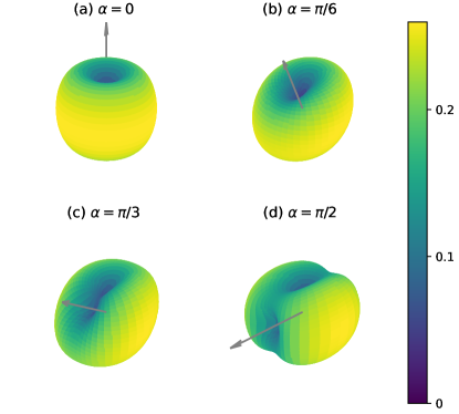
Figure 1: This figure depicts the antenna patterns, denoted as $\mathfrak{F}\left(\omega_{010},\theta,\phi\right)$ in Eq. 122, corresponding to magnetic field directions $\alpha\in\left\{0,\pi/6,\pi/3,\pi/2\right\}$ and an aspect ratio $L/R=1$. The gray arrows indicate the magnetic field directions. Antenna patterns for $\alpha>\pi/2$ can be obtained by rotating the patterns in the figure by $\pi$ around the axis of cylinder and reversing the direction of the gray arrows. This symmetry arises from the relation $\mathfrak{F}\left(\omega,\theta,\phi;\alpha\right)=\mathfrak{F}\left(\omega,\theta,\pi+\phi;\pi-\alpha\right)$.

V Summary and Discussion

We introduce physical laws in a globally hyperbolic spacetime described by Einstein’s equations. The contracted Bianchi identities imply the conservation of stress-energy. The congruence of the timelike geodesics without vorticity, have their spatial distribution determined by the extrinsic curvature. However, material elements, despite being influenced by gravity, deviate from geodesics due to elasticity stemming from their deformation. To account for the acoustic oscillation of the material, we introduce the 4-velocity and strain, both contributing the stress-energy. The equations of motion for these material elements encompass the temporal symmetry of the material metric, energy conservation, and the conservation of stress-energy. The EM field is governed by Maxwell’s equations. The electric and magnetic field to the material elements are determined by the 4-velocities of the elements. Considering the cavity as a vacuum, we impose the condition of vanishing spatial velocity and EM current. In cases where the material acts as a perfect conductor, the electric field is constrained to be orthogonal to the surface at the boundary.

For a concise discussion, we utilize covariant perturbation theory. Within this framework, we introduce the lemma that a linear perturbation is gauge-invariant if and only if the Lie derivative of its leading-order value vanishes along all directions. The perturbation of Einstein’s equations transforms into the wave equation for the Riemann tensor, where its wave solutions manifest as GWs. Utilizing these solutions, we present the perturbation of the timelike geodesic congruence. The perturbations of spatial velocity and strain for the material exhibit homogeneous and inhomogeneous wave equations, respectively, as dictated by their equations of motion. Perturbing Maxwell’s equations yield the wave equation for the perturbation of the electric field. Within the cavity, this equation indicates that GWs contribute to the perturbation of the electric field solely through the coupling between the EM field and the Riemann tensor. Lastly, we point out that fixing the 4-velocity of the material in a coordinate system or considering a rigid body within context of general relativity is not appropriate.

We solve Maxwell’s equations within the cavity. Using the solution for the electric field, we define the transfer function and the dimensionless GW signal. To derive the antenna pattern, we separate the GW signal into its strength and pattern function. Averaging the pattern function over the polarization angle yields the antenna pattern. As an illustrative example, we present the antenna pattern for the EM cavity using the TM010 mode at the resonance frequency.

Our work enables a profound understanding of the operational principles of GW detectors employing EM cavities by clearly elucidating the interplay among electric fields, acoustic oscillations, and GWs. Due to the generality of our analysis, it is relevant to various GW detectors employing EM fields. Our paper does not address the measurement principles and methods for the induced EM fields. We perceive this as a challenging problem, and it will be the focus of our future work.

References

• Abbott et al. (2023) R. Abbott, T. D. Abbott, F. Acernese, K. Ackley, C. Adams, N. Adhikari, R. X. Adhikari, V. B. Adya, C. Affeldt, D. Agarwal, et al., Physical Review X 13, 041039 (2023), ISSN 2160-3308.
• The EPTA and InPTA collaborations et al. (2023) The EPTA and InPTA collaborations, J. Antoniadis, S. Babak, A.-S. Bak Nielsen, and Al., Astronomy & Astrophysics (2023), ISSN 0004-6361, 1432-0746.
• Reardon et al. (2023) D. J. Reardon, A. Zic, R. M. Shannon, G. B. Hobbs, M. Bailes, V. Di Marco, A. Kapur, A. F. Rogers, E. Thrane, J. Askew, et al., The Astrophysical Journal Letters 951, L6 (2023), ISSN 2041-8205, 2041-8213.
• Agazie et al. (2023) G. Agazie, A. Anumarlapudi, A. M. Archibald, Z. Arzoumanian, P. T. Baker, B. Bécsy, L. Blecha, A. Brazier, P. R. Brook, S. Burke-Spolaor, et al., The Astrophysical Journal Letters 951, L8 (2023).
• Xu et al. (2023) H. Xu, S. Chen, Y. Guo, J. Jiang, B. Wang, J. Xu, Z. Xue, R. Nicolas Caballero, J. Yuan, Y. Xu, et al., Research in Astronomy and Astrophysics 23, 075024 (2023), ISSN 1674-4527.
• Herman et al. (2021) N. Herman, A. Fűzfa, L. Lehoucq, and S. Clesse, Physical Review D 104, 023524 (2021), ISSN 2470-0010, 2470-0029.
• Aggarwal et al. (2021) N. Aggarwal, O. D. Aguiar, A. Bauswein, G. Cella, S. Clesse, A. M. Cruise, V. Domcke, D. G. Figueroa, A. Geraci, M. Goryachev, et al., Living Reviews in Relativity 24, 4 (2021), ISSN 2367-3613, 1433-8351.
• Berlin et al. (2022) A. Berlin, D. Blas, R. T. D’Agnolo, S. A. R. Ellis, R. Harnik, Y. Kahn, and J. Schütte-Engel, Physical Review D 105, 116011 (2022), ISSN 2470-0010, 2470-0029.
• Domcke et al. (2022) V. Domcke, C. Garcia-Cely, and N. L. Rodd, Physical Review Letters 129, 041101 (2022), ISSN 0031-9007, 1079-7114.
• Andrew et al. (2023) K. Y. Andrew, S. Ahn, Ç. Kutlu, J. Kim, B. R. Ko, B. I. Ivanov, H. Byun, A. F. van Loo, S. Park, J. Jeong, et al., Physical Review Letters 130, 071002 (2023).
• Bartram et al. (2021) C. Bartram, T. Braine, E. Burns, R. Cervantes, N. Crisosto, N. Du, H. Korandla, G. Leum, P. Mohapatra, T. Nitta, et al., Physical review letters 127, 261803 (2021).
• Backes et al. (2021) K. M. Backes, D. A. Palken, S. A. Kenany, B. M. Brubaker, S. Cahn, A. Droster, G. C. Hilton, S. Ghosh, H. Jackson, S. K. Lamoreaux, et al., Nature 590, 238 (2021).
• Maggiore (2007) M. Maggiore, Gravitational Waves. Vol. 1: Theory and Experiments (Oxford University Press, 2007), ISBN 978-0-19-171766-6, 978-0-19-852074-0.
• Collaboration (2023) T. L. Collaboration, Monthly Notices of the Royal Astronomical Society 524, 5984 (2023), ISSN 0035-8711, eprint https://academic.oup.com/mnras/article-pdf/524/4/5984/52633671/stad588.pdf, URL https://doi.org/10.1093/mnras/stad588.
• Niikura et al. (2019) H. Niikura, M. Takada, S. Yokoyama, T. Sumi, and S. Masaki, Physical Review D 99, 083503 (2019), ISSN 2470-0010, 2470-0029.
• Wald (1984) R. M. Wald, General Relativity (University of Chicago Press, Chicago, IL, 1984), ISBN 0-226-87033-2.
• Hudelist et al. (2023) M. Hudelist, T. B. Mieling, and S. Palenta, Classical and Quantum Gravity 40, 085007 (2023), ISSN 0264-9381, 1361-6382.
• Gourgoulhon (2012) E. Gourgoulhon, 3+1 Formalism in General Relativity, vol. 846 (Springer Berlin Heidelberg, Berlin, Heidelberg, 2012), ISBN 978-3-642-24524-4.
• Hwang and Noh (2023) J.-c. Hwang and H. Noh, Annals of Physics 454, 169332 (2023), ISSN 00034916.
• Park (2022) C. Park, The Astrophysical Journal 940, 58 (2022), ISSN 0004-637X, 1538-4357.
• Stewart and Walker (1974) J. M. Stewart and M. Walker, Proceedings of the Royal Society of London. A. Mathematical and Physical Sciences 341, 49 (1974).
• Giulini (2010) D. Giulini, The Rich Structure of Minkowski Space (Springer Netherlands, Dordrecht, 2010), pp. 83–132, ISBN 978-90-481-3475-5, URL https://doi.org/10.1007/978-90-481-3475-5_4.