Abstract

String theory on $\text{AdS}_{3}\times\mathrm{S}^{3}\times\mathrm{T}^{4}$ geometries supported by a combination of NS-NS and R-R charges is believed to be integrable. We elucidate the kinematics and analytic structure of worldsheet excitations in mixed charge and pure NS-NS backgrounds, when expressed in momentum, Zhukovsky variables and the rapidity $u$ which appears in the quantum spectral curve. We discuss the relations between fundamental and bound state excitations and the role of fusion in constraining and determining the S matrices of these theories. We propose a scalar dressing factor consistent with a novel $u$-plane periodicity and comment on its close relation to the XXZ model at roots of unity. We solve the odd part of crossing and show that our solution is consistent with fusion and reduces in the relativistic limit to dressing phases previously found in the literature.

1 Introduction

The spectral problem of string theory on $\text{AdS}_{3}\times\mathrm{S}^{3}\times\mathrm{T}^{4}$ backgrounds is believed to be integrable [1, 2, 3]. Given any set of NS-NS and R-R charges and any value of moduli [6], an exact worldsheet S matrix satisfying the Yang-Baxter equation was constructed [7], by using the centrally-extended symmetries of the magnons in this theory. This generalises the findings for backgrounds with only R-R charge [8, 9, 10]. In all backgrounds supported by a mixture of NS-NS and R-R charge, the elementary worldsheet magnons have mass $m=1$ or $m=0$ and come in two type, denoted by L and R, in reference to their chirality in the dual $\text{CFT}_{2}$. Their exact dispersion relation [11, 7] is

$$E_{\mbox{\tiny L}}(p)=\sqrt{(m+\mathchar 22\relax\mkern-9.0mukp)^{2}+4h^{2}\sin^{2}\frac{p}{2}},\qquad E_{\mbox{\tiny R}}(p)=\sqrt{(m-\mathchar 22\relax\mkern-9.0mukp)^{2}+4h^{2}\sin^{2}\frac{p}{2}},$$ (1.1)

where

$$\mathchar 22\relax\mkern-9.0muk=\frac{k}{2\pi},$$ (1.2)

with $k\in\mathbb{Z}$ the level of the WZW term in the action. Above, $h$ is a function of the moduli of the mixed NS-NS and R-R charges, whose exact form remains to be determined, but whose leading order expressions are known [6]. When $\mathchar 22\relax\mkern-9.0muk$ is non-zero, the backgrounds have been referred to in the literature as mixed-flux, because at a generic point in moduli space both R-R and NS-NS fluxes are turned on in the supergravity solutions. As was clarified in [6], mixed-flux backgrounds include the theory supported by only NS-NS charge, for which at a generic point in moduli space the R-R three form flux is also non-zero due to the coupling to R-R axions. Turning off such axion moduli corresponds to setting $h=0$ and corresponds to the WZW point [13]. With this clarification implict, we will continue to use the term mixed-flux to refer to all backgrounds with $\mathchar 22\relax\mkern-9.0muk\neq 0$.

Unlike in the R-R theory [9], the mixed-flux dispersion relations (1.1) are no longer periodic in $p$ and physical momenta can take any real value. As a result, the kinematics of the excitations in mixed-flux theories is very different from the R-R cases. While momentum periodicity is broken, it is nevertheless useful to think of distinct momentum intervals, each with their own Zhukovsky sheets that can be reached through analytic continuation. While most of the Zhukovsky sheets share some similarities with the familiar R-R ones, they have important differences including a more complicated set of physical regions. In addition, there is one set of sheets which exhibits a novel type of periodicity. We explore these new features, in part using a visualisation programme [14] that is released together with this paper. For example, we find that the bound-state structure is novel compared to R-R theories, with bound states whose mass is larger than $k$ being identical to fundamental excitations with momentum on a different interval or equivalently on a different set of Zhukovsky sheets. This novel behaviour places important restrictions on the S matrices through fusion, relating for example the RL S matrix to the LL one.

This paper is organised as follows. In section 2, we disccuss in detail the mixed-flux Zhukovsky variables in terms of which the S matrix is most easily expressed, as well as the mixed-flux generalisation of the rapidity $u$, which has featured prominently in the quantum spectral curve (QSC) of R-R backgrounds [15, 16, 17, 18]. In section 3 we discuss the crossing transformations that place restricitions on the scalar factors of the S matrix and summarise our normalization conventions in section 4. In section 5, we review the R-R dressing factors proposed as solutions to the massive crossing equations in [10]. It was pointed out in [19] that these factors have unphysical logarithmic cuts in the Zhukovsky plane. Cavaglià and Ekhammar showed that these unwanted cuts can be removed in a straightforward way without spoiling the crossing or unitarity properites. This simple correction to [10] matches the dressing factors found in [19]. We review these findings in section 5, before solving the odd part [20] of the mixed-flux crossing equations in section 6. There, we also make proposals for the even scalar factors in the theory, which give rise to the expected bound state poles, but are trivial under crossing. Exploiting the periodicity on one of the sheets, we propose a scalar factor closely related to that of the XXZ model at a root of unity, i.e., with anisotropy of the form $\Delta=\cos\frac{\pi}{k}$. We show how in a relativistic limit, our results reduce to those found in [21]. Finally, in section 7 we discuss the bound-state analytic structure and fusion and show their compatibility with the odd dressing factors and the scalar factors we found. Finding the full even dressing factor which generalises the even part of the Beisert-Eden-Staudacher (BES) phase [20, 22] is beyond the scope of this paper and we hope to return to it in the near future.

2 Mixed-flux kinematics

The global symmetry of string theory on $\text{AdS}_{3}\times\mathrm{S}^{3}\times\mathrm{T}^{4}$ backgrounds is $\mathrm{psu}(1,1|2)^{2}$. When quantising the worldsheet theory in uniform light-cone gauge around the BMN vacuum, this is broken to $\mathrm{psu}(1|1)^{4}$. Each fundamental world-sheet excitation transforms in a short representation of a particular central extension of this algebra, conventionally denoted $\mathrm{psu}(1|1)^{4}_{\text{ce}}$. The dispersion relations (1.1) follow from the shoretening conditions, just as they do in integrable R-R backgrounds, see [23, 24] and references therein. In the pure R-R charge world-sheet theory ($\mathchar 22\relax\mkern-9.0muk=0$) the dispersion relation is periodic

$$E_{\text{R-R}}(p)=\sqrt{m^{2}+4h^{2}\sin^{2}\frac{p}{2}},$$ (2.1)

while in the pure NS-NS charge theory at the WZW point $(h=0)$, the dispersion relation reduces to a linear relativistic one

$$E_{\text{NS-NS}}(p)=|m+\mathchar 22\relax\mkern-9.0mukp|.$$ (2.2)

In contrast to the case of R-R backgrounds (for which $\mathchar 22\relax\mkern-9.0muk=0$), the mixed-flux dispersion relations are not periodic. There is instead a shift symmetry

$$p\to p\pm 2\pi,\qquad m\to m+k,$$ (2.3)

with $\pm=+$ for L representations and $\pm=-$ for R representations, discussed below. In this paper we are mainly concerned with fundamental excitations with mass $m=1$. Since the dispersion relation is no longer periodic, we allow for momenta of physical excitations to take any real value, rather than being restricted to the $\left[0,2\pi\right]$ interval familiar from integrable string theories with R-R flux. Analytic continuation in $p$ will then lead to a complex $p$ plane with cuts.

The L and R dispersion relations have branch points at complex values of momenta for which $E_{\mbox{\tiny L}}(p)=0$, respectively $E_{\mbox{\tiny R}}(p)=0$. The solutions of these equations, labelled $p^{(n)}_{b.p.}$, with $n\in\mathbb{Z}$ can be found numerically and come in complex conjugate pairs, with

$$\mbox{Re}\left(p_{b.p.}^{(n)}\right)\in\bigl{(}2\pi(n-\tfrac{1}{2}),2\pi(n+\tfrac{1}{2})\bigr{)}.$$ (2.4)

We choose the cuts to lie along the contours where $E_{\mbox{\tiny L}}(p)$ is imaginary, so the cuts do not cross the real $p$ axis as shown in figure 1. It is natural to think about these two sheets of the $p$ plane as a physical sheet, which contains the line where $p\in\mathbb{R}$ and $\mathop{\mathrm{Re}}E>0$, and a crossed sheet, containing the line $p\in\mathbb{R}$ and $\mathop{\mathrm{Re}}E<0$. However, as we will see later, once we consider bound states, not all physical (crossed) states fully sit on the physical (crossed) sheet of the $p$ plane.

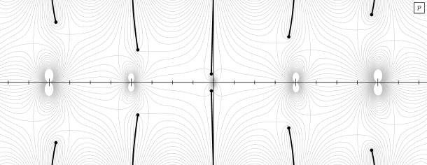
Figure 1: Location of branch points and branch cuts of $E_{L}(p)$. They come in complex conjugate pairs and we label each pair by an integer $n$, with the $n=0$ pair closest to the imaginary $p$-axis.

2.1 Zhukovsky variables

The mixed-flux dispersion relation and world-sheet S matrix take a simple form when expressed in terms of Zhukovsky variables. Since the theory is not parity invariant, these come in two types: $x_{\mbox{\tiny L}}^{\pm}$ and $x_{\mbox{\tiny R}}^{\pm}$, corresponding to two types of short representations L and R. Worldsheet energy and momentum can be expressed in terms of Zhukovsky variables in the same way as in the R-R case

$$e^{ip}=\frac{x_{\mbox{\tiny I}}^{+}}{x_{\mbox{\tiny I}}^{-}},\qquad E_{\mbox{\tiny I}}(p)=-\frac{ih}{2}\Bigl{(}x_{\mbox{\tiny I}}^{+}-\frac{1}{x_{\mbox{\tiny I}}^{+}}-x_{\mbox{\tiny I}}^{-}+\frac{1}{x_{\mbox{\tiny I}}^{-}}\Bigr{)},\qquad\mbox{I}=\mbox{L},\mbox{R}.$$ (2.5)

However, the L and R variables satisfy different shortening conditions

$$x_{\mbox{\tiny L}}^{+}+\frac{1}{x_{\mbox{\tiny L}}^{+}}-x_{\mbox{\tiny L}}^{-}-\frac{1}{x_{\mbox{\tiny L}}^{-}} =\frac{2i(m+\mathchar 22\relax\mkern-9.0mukp)}{h},$$ (2.6)

$$x_{\mbox{\tiny R}}^{+}+\frac{1}{x_{\mbox{\tiny R}}^{+}}-x_{\mbox{\tiny R}}^{-}-\frac{1}{x_{\mbox{\tiny R}}^{-}} =\frac{2i(m-\mathchar 22\relax\mkern-9.0mukp)}{h}.$$

Focussing on the L representations, from (2.5) we find that an excitation with real momentum and positive energy has $x_{\mbox{\tiny L}}^{+}$ in the upper half-plane and $x_{\mbox{\tiny L}}^{-}=(x_{\mbox{\tiny L}}^{+})^{*}$. The shortening condition is then solved by

$$x_{\mbox{\tiny L}}^{\pm}(p,m)=\Xi_{\mbox{\tiny L}}^{\pm}(p,m)\equiv\frac{m+\mathchar 22\relax\mkern-9.0mukp+\sqrt{(m+\mathchar 22\relax\mkern-9.0mukp)^{2}+4h^{2}\sin^{2}\frac{p}{2}}}{2h\sin\frac{p}{2}}e^{\pm\frac{ip}{2}}.$$ (2.7)

We often drop the arguments of $x_{\mbox{\tiny L}}^{\pm}$ and, unless otherwise specified, we then consider the case of a fundamental excitation with $m=1$.

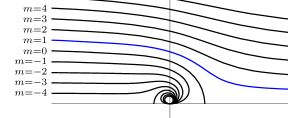
(a) $\Xi_{\mbox{\tiny L}}^{+}(p,m)$

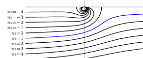
(b) $\Xi_{\mbox{\tiny L}}^{-}(p,m)$

Figure 2: Plots of the functions $\Xi_{\mbox{\tiny L}}^{\pm}(p,m)$ with $m=-8,\dots,6$ and $p\in[0,2\pi]$. In the $\Xi_{\mbox{\tiny L}}^{+}(p,m)$ ($\Xi_{\mbox{\tiny L}}^{-}(p,m)$) plot the top (bottom) curve has $m=6$ and $m$ decreases as one moves to lower (higher) curves, with the smallest oval curve shown having $m=-8$. Non-integer values of $m$ will fill the remaining parts of each half-plane. The blue curves have $m=1$ and shows the location of fundamental excitations with $p\in[0,2\pi]$.

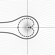
(a) $h=7$, $k=3$

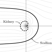
(b) $h=2$, $k=5$

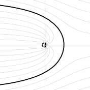
(c) $h=1$, $k=7$

Figure 3: The scallion and kidney contours for various values of the couplings.

The functions $\Xi_{\mbox{\tiny L}}^{\pm}(p,m)$ appearing on the right hand side of (2.7) can also be used to cover the Zhukovsky planes. To do this we consider $m\in\mathbb{R}$ and because of the symmetry (2.3), we can restrict to $p\in[0,2\pi]$. In figure 2 we plot $\Xi_{\mbox{\tiny L}}^{\pm}(p,m)$ for $m=-8,\dots,6$ and $p\in[0,2\pi]$. From the figure it should be clear that with $m\in\mathbb{R}$, $\Xi_{\mbox{\tiny L}}^{+}(p,m)$ covers the UHP while $\Xi_{\mbox{\tiny L}}^{-}(p,m)$ covers the LHP. We may view the parameter $m$ as a type of radial ordering of the Zhukovsky planes.

For later convenience we also introduce the related function

$$\tilde{\Xi}_{\mbox{\tiny L}}^{\pm}(p,m)=\frac{m+\mathchar 22\relax\mkern-9.0mukp-\sqrt{(m+\mathchar 22\relax\mkern-9.0mukp)^{2}+4h^{2}\sin^{2}\frac{p}{2}}}{2h\sin\frac{p}{2}}e^{\pm\frac{ip}{2}},$$ (2.8)

which solves the L shortening condition when $\mathop{\mathrm{Re}}E_{\mbox{\tiny L}}(p)<0$, as well as the functions

$$\Xi_{\mbox{\tiny R}}^{\pm}(p,m) =\frac{m-\mathchar 22\relax\mkern-9.0mukp+\sqrt{(m-\mathchar 22\relax\mkern-9.0mukp)^{2}+4h^{2}\sin^{2}\frac{p}{2}}}{2h\sin\frac{p}{2}}e^{\pm\frac{ip}{2}},$$ (2.9)

$$\tilde{\Xi}_{\mbox{\tiny R}}^{\pm}(p,m) =\frac{m-\mathchar 22\relax\mkern-9.0mukp-\sqrt{(m-\mathchar 22\relax\mkern-9.0mukp)^{2}+4h^{2}\sin^{2}\frac{p}{2}}}{2h\sin\frac{p}{2}}e^{\pm\frac{ip}{2}},$$

which solve the R shortening conditions when $\mathop{\mathrm{Im}}E_{\mbox{\tiny R}}(p)>0$ and $\mathop{\mathrm{Im}}E_{\mbox{\tiny R}}(p)<0$, respectively.

The contours $\Xi_{\mbox{\tiny L}}^{\pm}(p,m=0)$ and $\Xi_{\mbox{\tiny L}}^{\pm}(p,m=-k)$, which are shown in figure 3, play a distinguished role in the Zhukovsky planes, since they correspond to the branch cuts in the rapidity plane. We find their form reminiscent of scallion and a kidney and we will often refer to these curves as such.

For a given real momentum $p^{\prime}\in[0,2\pi]$ and real mass $m^{\prime}$ there is an infinite number of complex momenta $p$ such that $x_{\mbox{\tiny L}}^{+}(p,m=1)=\Xi_{\mbox{\tiny L}}^{+}(p^{\prime},m^{\prime})$ and also an infinite number of (separate) complex momenta $p$ such that $x_{\mbox{\tiny L}}^{+}(p,m=1)=\Xi_{\mbox{\tiny L}}^{-}(p^{\prime},m^{\prime})$. The same holds for the equations $x_{\mbox{\tiny L}}^{-}(p,m=1)=\Xi_{\mbox{\tiny L}}^{\pm}(p^{\prime},m^{\prime})$. To illustrate this, figure 4a on page 4a shows the $p$ plane with contours labelled by $m^{\prime}\in\mathbb{Z}$ such that $x_{\mbox{\tiny L}}^{+}(p,m=1)=\Xi_{\mbox{\tiny L}}^{+}(p^{\prime},m^{\prime})$ or $x_{\mbox{\tiny L}}^{+}(p,m=1)=\Xi_{\mbox{\tiny L}}^{-}(p^{\prime},m^{\prime})$ for some real $p^{\prime}\in[0,2\pi]$. Figure 4b shows the corresponding plot for $x_{\mbox{\tiny L}}^{-}(p,m=1)$. In the figures we have also indicated the curves mapping to the real line of the $x_{\mbox{\tiny L}}^{\pm}$ planes, as well as the pre-images of the scallion and kidney contours. The distinguished role of these contours can be seen in the figures: in the $x_{\mbox{\tiny L}}^{+}$ plot in figure 4a there is a branch point where the $x_{\mbox{\tiny L}}^{-}$ scallion or kidney intersects with the $x_{\mbox{\tiny L}}^{-}$ real line. The nature of these branch points is best understood through the $u$ plane which we will introduce next.

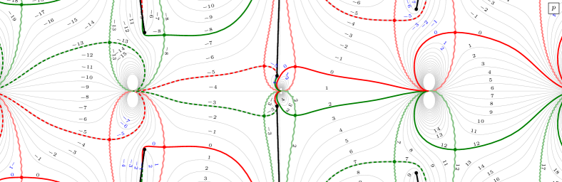
(a) $x_{\mbox{\tiny L}}^{+}(p,m=1)=\Xi^{\pm}(p^{\prime},m^{\prime})$

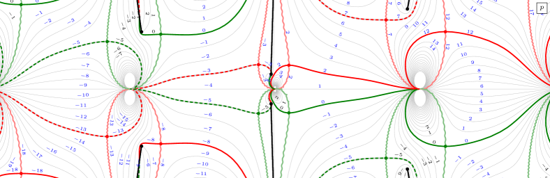
(b) $x_{\mbox{\tiny L}}^{+}(p,m=1)=\Xi^{\pm}(p^{\prime},m^{\prime})$

Figure 4: Plots of the complex $p$ plane with contours labelled by $m^{\prime}\in\mathbb{Z}$ such that $x_{\mbox{\tiny L}}^{\pm}(p,m=1)=\Xi_{\mbox{\tiny L}}^{+}(p^{\prime},m^{\prime})$ (in black) or $x_{\mbox{\tiny L}}^{\pm}(p,m=1)=\Xi_{\mbox{\tiny L}}^{-}(p^{\prime},m^{\prime})$ (in blue). The wavy red and green lines show the pre-image of the real line in the $x_{\mbox{\tiny L}}^{+}$ and $x_{\mbox{\tiny L}}^{-}$ lines. We also indicate the location of the $x_{\mbox{\tiny L}}^{+}$/$x_{\mbox{\tiny L}}^{-}$ scallion with solid red/green curves, and the kidneys with corresponding dashed curves.

2.2 The $u$-plane

Another variable that is often useful in integrable holographic models is the rapidity $u$. In the mixed-flux setting this is defined as [11]

$$u_{\mbox{\tiny L}}(x)=x+\frac{1}{x}-\frac{2\mathchar 22\relax\mkern-9.0muk}{h}\log x,\qquad u_{\mbox{\tiny R}}(x)=x+\frac{1}{x}+\frac{2\mathchar 22\relax\mkern-9.0muk}{h}\log x.$$ (2.10)

The shortening conditions (2.6) can then be written as

$$u_{\mbox{\tiny L}}(x_{\mbox{\tiny L}}^{+})-u_{\mbox{\tiny L}}(x_{\mbox{\tiny L}}^{-})=\frac{2im}{h},\qquad u_{\mbox{\tiny R}}(x_{\mbox{\tiny R}}^{+})-u_{\mbox{\tiny R}}(x_{\mbox{\tiny R}}^{-})=\frac{2im}{h}.$$ (2.11)

It is then natural the introduce the rapidities $u_{\mbox{\tiny L}}$ and $u_{\mbox{\tiny R}}$ such that

$$u_{\mbox{\tiny L}}(x_{\mbox{\tiny L}}^{\pm})=u_{\mbox{\tiny L}}\pm\frac{im}{h},\qquad u_{\mbox{\tiny R}}(x_{\mbox{\tiny R}}^{\pm})=u_{\mbox{\tiny R}}\pm\frac{im}{h}.$$ (2.12)

By solving $\frac{du}{dx}=0$ we find that the branch points of $x_{\mbox{\tiny L}}(u_{\mbox{\tiny L}})$ are at

$$x^{\mbox{\scriptsize b.p.}}_{L}=s,\,-s^{-1},$$ (2.13)

while those of $x_{\mbox{\tiny R}}(u_{\mbox{\tiny R}})$ are at

$$x^{\mbox{\scriptsize b.p.}}_{R}=-s,\,s^{-1},$$ (2.14)

where, following [25], we have introduced the parameter $s$

$$\frac{\mathchar 22\relax\mkern-9.0muk}{h}=\frac{s-s^{-1}}{2},$$ (2.15)

with $s\geq 1$, in which case

$$s=\frac{\mathchar 22\relax\mkern-9.0muk+\sqrt{h^{2}+\mathchar 22\relax\mkern-9.0muk^{2}}}{h},\qquad\qquad-s^{-1}=\frac{\mathchar 22\relax\mkern-9.0muk-\sqrt{h^{2}+\mathchar 22\relax\mkern-9.0muk^{2}}}{h}.$$ (2.16)

2.2.1 The analytical structure of $u_{\mbox{\tiny L}}(x_{\mbox{\tiny L}})$

The function $u_{\mbox{\tiny L}}(x_{\mbox{\tiny L}})$ has a fairly complicated analytical structure. The inverse function $x_{\mbox{\tiny L}}(u_{\mbox{\tiny L}})$ has branch points at $x_{\mbox{\tiny L}}=s$ and $x_{\mbox{\tiny L}}=-1/s$. Additionally $u_{\mbox{\tiny L}}(x_{\mbox{\tiny L}})$ itself has a log cut which sits on the negative real axis of the $x_{\mbox{\tiny L}}$ plane. Together this means that we will need an infinite number of sheets in both the $x_{\mbox{\tiny L}}$ plane and the $u_{\mbox{\tiny L}}$ plane to describe the full function.

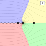
(a) The $x_{\mbox{\tiny L}}$ plane with long cuts.

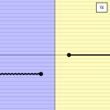
(b) Sheet covering the upper half of the $x_{\mbox{\tiny L}}$ plane.

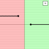
(c) Sheet covering the lower half of the $x_{\mbox{\tiny L}}$ plane.

Figure 5: The $u_{\mbox{\tiny L}}$ plane with long cuts.

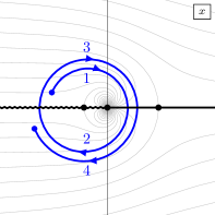
Figure 6: A path wrapping twice around the origin of $x_{\mbox{\tiny L}}$.

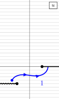
(a)

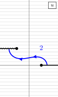
(b)

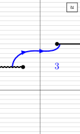
(c)

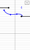
(d)

Figure 7: Four sheets of $u_{\mbox{\tiny L}}$ with long cuts.

Let us first see what it takes to cover a single sheet of the $x_{\mbox{\tiny L}}$ plane. A simple choice is to use “long” cuts, where the upper and lower half of the $x_{\mbox{\tiny L}}$ planes are completely covered by one sheet of the $u_{\mbox{\tiny L}}$ plane each. Figure 5a shows the $x_{\mbox{\tiny L}}$ plane with long cuts and figure 5b and 5c show the two corresponding sheets of the $u_{\mbox{\tiny L}}$ plane. As is clear from the picture, the two sheets are connected by the cut on the right. If we instead go through the left cut, we simultaneously go through the log cut in the $x_{\mbox{\tiny L}}$ plane and thus come out on a new sheet of the $x_{\mbox{\tiny L}}$ plane, which comes with two new $u_{\mbox{\tiny L}}$ sheet.

To see this in more detail, figure 6 shows a path that wraps twice around the origin in the $x_{\mbox{\tiny L}}$ plane. In the $u_{\mbox{\tiny L}}$ plane this corresponds to the path in figure 7.

A benefit of the long cuts is that each sheet of the $x_{\mbox{\tiny L}}$ plane is completely covered by two full sheets of the $u_{\mbox{\tiny L}}$ plane. However, in what follows we will find it more convenient to work with “short” cuts. These can be thought of as the complement of the long cuts. We cut each sheet of the $u_{\mbox{\tiny L}}$ plane into three pieces along horizontal lines coincident with the long cuts, and then glue them back together along the opposite cuts. This partitions the $x_{\mbox{\tiny L}}$ plane into a region outside the scallion, and region between the scallion and the kidney, and a region inside the kidney, as shown in figures 8a, 8b and 8c, respectively. The inside region is further split into an upper and a lower part by the log cut.

If we only consider a single sheet of the $x_{\mbox{\tiny L}}$ plane, the short cuts split the $u_{\mbox{\tiny L}}$ plane into four parts. The outside region is covered by one sheet of $u_{\mbox{\tiny L}}$ with a single cut, see figure 8d. The between region corresponds to a horizontal strip of height $2k/h$, see figure 8e and the inside region corresponds to two disconnected and offset half-planes, see figure 8f.

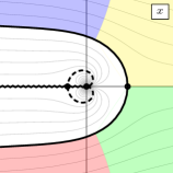
(a)

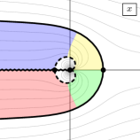
(b)

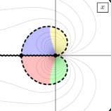
(c)

(d)

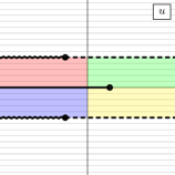
(e)

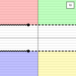
(f)

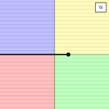
(g)

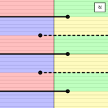
(h)

(i)

Figure 8: The $x$ and $u$ planes with “short” cuts split into regions outside the scallion (figures LABEL:sub@fig:x-region-outside, LABEL:sub@fig:u-region-outside-small and LABEL:sub@fig:u-region-outside), between the scallion and the kidney (figures LABEL:sub@fig:x-region-between, LABEL:sub@fig:u-region-between-small and LABEL:sub@fig:u-region-between) and inside the kidney (figures LABEL:sub@fig:x-region-inside, LABEL:sub@fig:u-region-inside-small and LABEL:sub@fig:u-region-inside). When entering a cut in the $u$ plane we come out on the next sheet in a region with the same colour. The middle figures LABEL:sub@fig:u-region-outside-small, LABEL:sub@fig:u-region-between-small and LABEL:sub@fig:u-region-inside-small show the parts of the $u_{\mbox{\tiny L}}$ plane with short cuts that cover a single sheet of the $x_{\mbox{\tiny L}}$ plane. The last row, with figures LABEL:sub@fig:u-region-outside, LABEL:sub@fig:u-region-between and LABEL:sub@fig:u-region-inside, shows three sheets of the $u_{\mbox{\tiny L}}$ plane after extending them through the log cuts.

However, we can now easily extend the $u_{\mbox{\tiny L}}$ plane through the log cuts in the between and inside regions. We then find that the between region gives rise to a periodic $u_{\mbox{\tiny L}}$ sheet as in figure 8h while the region inside the kidney corresponds to a sheet with a single cut as in figure 8i. With short cuts the log cut is thus completely resolved in the $u_{\mbox{\tiny L}}$ plane. As an example of this figure 9 shows the same path as in figures 6 and 7. With short cuts the whole path sits on a single sheet.

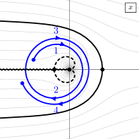
(a)

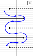
(b)

Figure 9: A path encircling the origin of the $x_{\mbox{\tiny L}}$ plane. The short cuts resolve the log cut.

2.2.2 The full $u_{\mbox{\tiny L}}$ plane

In the previous section we considered the analytical structure of the function $u_{\mbox{\tiny L}}(x_{\mbox{\tiny L}})$ and its inverse. However, to describe the full kinematics of the mixed-flux string theory we need both Zhukovsky variables $x_{\mbox{\tiny L}}^{\pm}$. The full $u_{\mbox{\tiny L}}$ plane therefore has twice the number of cuts to what was discussed above. Let us illustrate this by considering a path in the momentum plane that goes from $(0,2\pi)$ to $(-2\pi,0)$ as shown in figure 10a on page 10a. Its images in the $x^{+}$ and $x^{-}$ planes, drawn for compactness together in figure 10b, split into four parts:

1. $x^{\pm}$ start out with real momentum $p\in[0,2\pi]$ and $x^{+}$ is brought inside the scallion from below,

2. $x^{-}$ is brought inside the scallion,

3. $x^{+}$ goes through the log cut,

4. $x^{\pm}$ end up with real momentum $p\in[-2\pi,0]$.

Figures 10c–LABEL:sub@fig:u-simple-path-34 shows the same path in the $u$ plane. For real momentum $p\in[0,2\pi]$ there are two cuts corresponding to $x^{+}$ and $x^{-}$ going through the scallion. In the first step (figure 10c) we go through the $x^{+}$ scallion cut. We then come out on a new sheet (figure 10d) where we have a periodic set of $x^{+}$ cuts (in red) but a single $x^{-}$ cut (in green). We go through the $x^{-}$ cut. Finally, we come out (figure 10e) on a third sheet where both the red $x^{+}$ cuts and the green $x^{-}$ cuts are periodic. Since the $u$ plane resolves the log cut we can just go up to the real momentum line. Note that for real momentum $p\in[0,2\pi]$ we have chosen $u$ to be real. As we have just seen, this means that for $p\in[-2\pi,0]$ $u$ will not be real.

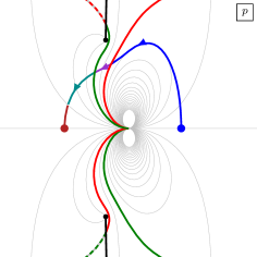
(a)

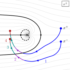
(b)

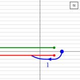
(c)

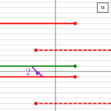
(d)

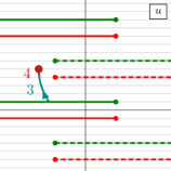
(e)

Figure 10: A simple path that takes $x^{\pm}$ from the outside of the scallion to the region between the scallion and the kidney.

Consider next a path in the $p$ plane that begins and ends on $(0,2\pi)$ and goes clockwise around $p=0$ as shown in figure 11a. The image of this path in the $x^{+}$ and $x^{-}$ planes, again drawn for compactness together in figure 11b where both $x^{+}$ and $x^{-}$ encircle the origin as well as the branch points at $s$ and $-1/s$ once in a anti-clockwise direction. The corresponding path in the $u$ plane is shown in figure 11c–LABEL:sub@fig:u-large-circle-3. From the point of view of $x^{\pm}$, the path takes us back to the exact same point we started at, but that is not true in the $u$ plane. Instead, the end point sits on a sheet which looks identical to the one we started on except everything is shifted down by $2ik/h$. If instead we had gone around $p=0$ in an anti-clockwise direction, we would have ended up on a $u$ sheet where everything is shifted up by $2ik/h$. This argument shows that it is only the difference of $u(x^{+})$ and $u(x^{-})$ that is physical, rather than the value of each.

(a)

(b)

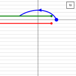
(c)

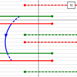
(d)

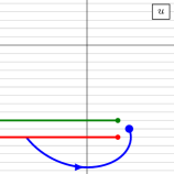
(e)

Figure 11: A path describing a large circle in the $x^{+}$ plane.

We can also think about separate $x^{+}$ and $x^{-}$ planes, where in, e.g., the $x^{+}$ plane we include not only the normal scallion and kidney, but also additional cuts where $x^{-}$ goes through the scallion and the kidney. See figure 12 where we have also included the image of the $E(p)$ cut of the $p$ plane as a black line.

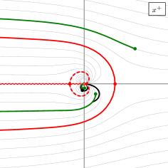
(a)

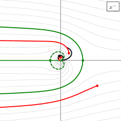
(b)

Figure 12: The full $x^{+}$ and $x^{-}$ planes as seen by an excitation with $p\in(0,2\pi)$.

2.3 The $p$, $x^{\pm}$ and $u$ planes

We are now finally ready to discuss the full analytical structure of the $p$, $x^{+}$, $x^{-}$ and $u$ planes. Let us start by summarising the types of cuts we encounter in the various planes:

1. The $\boldsymbol{p}$ plane has two sheets connected by an infinite number of $E(p)$ cuts.

2. The $\boldsymbol{x^{\pm}}$ planes have an infinite number of sheets. The sheets are connected both through log cuts, along the negative real axis, and through the $x^{\mp}$ scallion and kidney cuts.

3. The $\boldsymbol{u}$ plane has an infinite number of sheets connected through the $x^{\pm}$ scallion and kidney cuts.

A physical excitation with real momentum $p$ (by definition) sits along the real line on the first sheet of the $p$ plane. It is natural to divide this real line into regions $(2\pi n,2\pi(n+1))$. This corresponds to $x_{\mbox{\tiny L}}^{-}=(x_{\mbox{\tiny L}}^{+})^{*}$ with $\mathop{\mathrm{Im}}x_{\mbox{\tiny L}}^{+}>0$ and $u_{\mbox{\tiny L}}$ along a line with $\mathop{\mathrm{Im}}u_{\mbox{\tiny L}}=kl/h$ for some $l\in\mathbb{Z}$, where $l$ is an even (odd) integer when $n$ is even (odd).

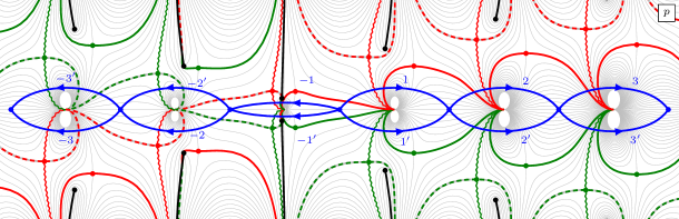
Figure 13: To go from real momentum $p\in(2\pi n,2\pi(n+1))$ to momentum $p+2\pi$ or $p-2\pi$ we need to choose if we go above or below the point $2\pi(n+1)$ or $2\pi n$, respectively. Equivalently we need to choose if we go through the log cut in the $x_{\mbox{\tiny L}}^{+}$ or $x_{\mbox{\tiny L}}^{-}$ plane. The paths $-3,-2,\dotsc,3$ all cross the $x_{\mbox{\tiny L}}^{+}$ log cut while the paths $-3^{\prime},-2^{\prime},\dotsc,3^{\prime}$ cross the $x_{\mbox{\tiny L}}^{-}$ log cut.

When $p$ approaches a multiple of $2\pi$ $x_{\mbox{\tiny L}}^{\pm}$ and $u_{\mbox{\tiny L}}$ all diverge. In order to continuously go between the different real momentum regions we need to go into the complex plane. At each point $2\pi n$ we need to choose if we go above or below the point. Some such paths are illustrated in figure 13. Let us first consider going from the region 0 (with $p\in(0,2\pi)$) to the region 1 (with $p\in(2\pi,4\pi)$). The figure shows two paths:

1. Take $x_{\mbox{\tiny L}}^{+}$ into the scallion, through the log cut and then out of the scallion again.

2. Take $x_{\mbox{\tiny L}}^{-}$ into the scallion, through the log cut and then out of the scallion again.

In either case the other parameter ($x_{\mbox{\tiny L}}^{\mp}$) stays outside the scallion. Once we go down to the real momentum line again we find that $x_{\mbox{\tiny L}}^{\pm}$ are now located on the

$$x_{\mbox{\tiny L}}^{\pm}=\Xi_{\mbox{\tiny L}}^{\pm}(p-2\pi,m=k+1)$$ (2.17)

contours, where we write the momentum as $p-2\pi$ to emphasise that $x_{\mbox{\tiny L}}^{\pm}$ has momentum in the $(2\pi,4\pi)$ range while the functions $\Xi_{\mbox{\tiny L}}^{\pm}(p,m)$ were define for $p\in(0,2\pi)$. Going to higher momentum regions along the paths $2,3,\dotsc$ or $2^{\prime},3^{\prime},\dotsc$ is just repeating a similar path.

To go to the $-1$ region (where $p\in(-2\pi,0)$) we take both $x_{\mbox{\tiny L}}^{+}$ and $x_{\mbox{\tiny L}}^{-}$ through both scallions, see path $-1$ and $-1^{\prime}$ in the figure. The region $-2$ (where $p\in(-4\pi,-2\pi)$) takes us into the kidney, and to go to yet lower regions we just take one of $x_{\mbox{\tiny L}}^{\pm}$ out of the kidney, through the log cut and then back in to the kidney again.

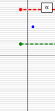
(a) $n=-3$

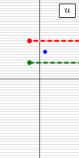
(b) $n=-2$

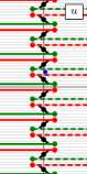
(c) $n=-1$

(d) $n=0$

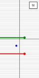
(e) $n=1$

(f) $n=2$

Figure 14: The physical region in the $u$ plane for various momentum regions $2\pi n<p<2\pi(n+1)$. The blue dots correspond to excitations with real momenta $p=2\pi n+\pi$. The real momentum line in the middle of the cuts. The $u$ plane for $n=-1$ is periodic and shows an infinite number of both scallion and kidney cuts. The other regions each have two cuts.

It seems natural to pick a convention where we always take say $x_{\mbox{\tiny L}}^{+}$ through the log cut. This means that we go around the point $p=2\pi n$ in the upper half-plane for $n\geq 0$ and in the lower half-plane for $n<0$. In the $u_{\mbox{\tiny L}}$ plane real momenta in region $n$ then correspond to $\mathop{\mathrm{Im}}u_{\mbox{\tiny L}}=-\frac{nk}{h}$. Moreover, for $n\geq 0$ the $x_{\mbox{\tiny L}}^{-}$ scallion cut in the $u_{\mbox{\tiny L}}$ plane will be in a fixed position with imaginary part $+1/h$, with the $x_{\mbox{\tiny L}}^{+}$ scallion cut at $-(2nk+1)/h$, and for $n<-1$ the $x_{\mbox{\tiny L}}^{-}$ kidney cut will always have imaginary part $(k+1)/h$, with the $x_{\mbox{\tiny L}}^{+}$ kidney cut at $-((2n+1)k+1)/h$, see figure 14.

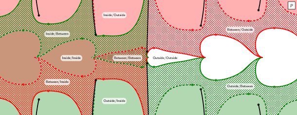
(a) The sheet $\mathop{\mathrm{Re}}E>0$

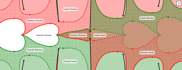
(b) The sheet $\mathop{\mathrm{Re}}E<0$

Figure 15: The $p$ plane can be naturally subdivided into regions depending on the location of $x_{\mbox{\tiny L}}^{\pm}$. If $x_{\mbox{\tiny L}}^{+}$ ($x_{\mbox{\tiny L}}^{-}$) is inside the kidney the region is filled with a solid red (green) colour, if $x_{\mbox{\tiny L}}^{+}$ ($x_{\mbox{\tiny L}}^{-}$) is between the scallion and the kidney the region is filled with a diagonal red (green) pattern, and if $x_{\mbox{\tiny L}}^{+}$ ($x_{\mbox{\tiny L}}^{-}$) is outside the scallion we leave the region unfilled. The colours mix, so that, e.g., a solid brownish colour means that $x_{\mbox{\tiny L}}^{\pm}$ are both inside the kidney and a solid green colour means that $x_{\mbox{\tiny L}}^{+}$ is outside the scallion and $x_{\mbox{\tiny L}}^{-}$ is inside the kidney.

The scallion and kidney cuts naturally partition the $p$ planes into regions depending on where $x_{\mbox{\tiny L}}^{+}$ and $x_{\mbox{\tiny L}}^{-}$ sit: outside the scallion, between the scallion and kidney, or inside the kidney, as illustrated in figure 15.

For an excitation with real momentum, $x_{\mbox{\tiny L}}^{\pm}$ sit in the same region. In particular, if the momentum $p$ is in the range $(2\pi n,2\pi(n+1))$, a physical excitation, which has positive energy and sits on the real line of the first sheet of the $p$ plane, has

$$x_{\mbox{\tiny L}}^{\pm}(p,1)=\Xi_{\mbox{\tiny L}}^{\pm}(p-2\pi n,1+nk)$$ (2.18)

while a crossed excitation, with negative energy sitting on the real line of the second sheet of the $p$ plane, has

$$x_{\mbox{\tiny L}}^{\pm}(p,1)=\Xi_{\mbox{\tiny L}}^{\mp}\bigl{(}2\pi(n+1)-p,-1-(n+1)k\bigr{)}.$$ (2.19)

As a result, a crossed real momentum excitation has $x_{\mbox{\tiny L}}^{-}$ in the upper half-plane and $x_{\mbox{\tiny L}}^{+}$ in the lower half-plane.

2.4 Bound states

In addition to fundamental excitations the world-sheet spectrum contains bound states of such excitations. The basic construction of such bound states follows from $\mathrm{psu}(1|1)^{4}_{\text{ce}}$ representation theory and is the same as in the pure R-R theory [26, 27, 28]. An $m$-particle boundstate has $m$ constituent Zhukovsky parameters $x_{j}^{\pm}$, $j=1,\dotsc,m$ satisfying

$$x_{j}^{-}=x_{j+1}^{+},\quad j=1,\dotsc,m-1.$$ (2.20)

The bound state condition (2.20) ensures that the momentum, energy and charge of the bound state only depends on the “outer-most” Zhukovsky parameters $X^{+}=x_{1}^{+}$ and $X^{-}=x_{1}^{-}$. Using (2.5) we have

$$E_{\text{tot}}=\sum_{j=1}^{m}E_{j}=-\frac{ih}{2}\sum_{j=1}^{m}x_{j}^{+}-\frac{1}{x_{j}^{+}}-x_{j}^{-}+\frac{1}{x_{j}^{-}}=-\frac{ih}{2}\Bigl{(}X^{+}-\frac{1}{X^{+}}-X^{-}+\frac{1}{X^{-}}\Bigr{)},$$ (2.21)

and

$$e^{ip_{\text{tot}}}=\frac{X^{+}}{X^{-}}=\prod_{j=1}^{m}\frac{x_{j}^{+}}{x_{j}^{-}}\equiv\prod_{j=1}^{m}e^{ip_{j}},$$ (2.22)

where $p_{j}$ is the momentum of the $j$-th constituent of the bound state. From the shortening condition (2.6) we find the charge

$$m+\mathchar 22\relax\mkern-9.0mukp_{\text{tot}}=-\frac{ih}{2}\sum_{j=1}^{m}x_{j}^{+}+\frac{1}{x_{j}^{+}}-x_{j}^{-}-\frac{1}{x_{j}^{-}}=-\frac{ih}{2}\Bigl{(}X^{+}+\frac{1}{X^{+}}-X^{-}-\frac{1}{X^{-}}\Bigr{)}.$$ (2.23)

$X^{\pm}$ thus satisfy the L shortening condition (2.6).

In the $u_{\mbox{\tiny L}}$ plane the bound state condition (2.20) translates to a simple Bethe string configuration of the form

$$u_{j+1}=u_{j}-\frac{2i}{h},$$ (2.24)

where

$$u_{j}\pm\frac{i}{h}\equiv u(x^{\pm}_{j}),$$ (2.25)

like in the pure R-R case.

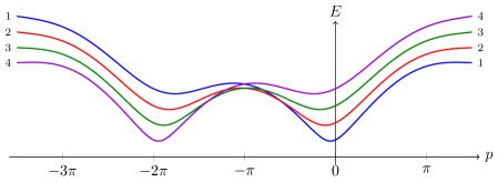
Figure 16: Bound state dispersion relations for $h=2$, $k=5$ and $m=1,\dotsc,k-1$. Note that for negative momentum $p$ and small bound state numbers $m$ the energy is decreasing as $m$ increases.

It is worth stressing a feature of the bound state dispersion relation

$$\sqrt{(m+\mathchar 22\relax\mkern-9.0mukp)^{2}+4h^{2}\sin^{2}\frac{p}{2}}.$$ (2.26)

In figure 16 we have plotted the dispersion relation of bound states with $m=1,\dotsc,k-1$ for $k=5$. We note that for $p>0$ the energy increases with increasing $m$, as happens in conventional relativistic theories and in R-R integrable backgrounds. However, as $p$ is lowered from $0$ to $-2\pi$ the energy levels cross each other, and for $p<-2\pi$ the energy decreases as $m$ increases from $1$ to $k-1$.

Bound states with $p\in(0,2\pi)$.

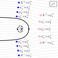
(a) $0<p<2\pi$

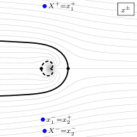
(b) $2\pi<p<4\pi$

Figure 17: Typical configurations corresponding to bound states. Figure LABEL:sub@fig:x-boundstates-0 shows two bound states with momentum $p\in(0,2\pi)$. The filled dots on the right show the locations of the five parameters $x_{1}^{\pm},\dotsc,x_{5}^{\pm}$ making up a bound state with $m=7$. Similarly, the hollow dots on the rights show the locations of the four parameters describing a bound state with $m=4$. Figure LABEL:sub@fig:x-boundstates-1 shows a bound state with $m=2$ and $p\in(2\pi,4\pi)$.

Figure 17a shows two typical bound states with $m=4$ and $m=7$ and total momentum $p$ in the $(0,2\pi)$ range. The highest component sits at $x_{1}^{+}=X^{+}=\Xi_{\mbox{\tiny L}}^{+}(p,m)$. The next component sits two steps below that, at $x_{1}^{-}=x_{2}^{+}=\Xi^{+}(q_{1},m-2)$, where $q_{1}$ is a real parameter which can be determined through the shortening condition for $x_{1}^{\pm}$. The subsequent excitations sit along curves below this, with $m$ decreasing in steps of two, until we reach the lowest component $x_{m}^{-}=X^{-}=\Xi_{\mbox{\tiny L}}^{-}(p,m)$. In this way we can construct simple bound states with total momentum in the $(0,2\pi)$ range, and with all constituents having (complex) momenta in the same range.

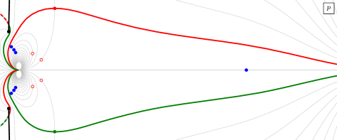
Figure 18: $p$ plane plot of two bound states with momentum in $(0,2\pi)$.

Figure 18 shows the same two states as in figure 17a but in the $p$ plane. From conventional relativistic intuition of bound states one might expect that energy and momentum should be more or less evenly distributed among the constituents. This is indeed true for the $m=4$ states represented by the red hollow circles, because this state has relatively small total momentum. However, as we increase total momentum, most of the energy and momentum is carried by a single excitation as in the $m=7$ state represented by the blue dots in the figure. Indeed, we can see that any excitation sitting on a contour $\Xi_{\mbox{\tiny L}}^{\pm}(p,m)$ with $m>2$ is confined to a small region close to the origin in the $p$ plane.

Bound states with $p>2\pi$.

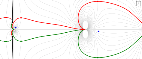
Figure 19: A two particle bound state with total momentum in $(2\pi,4\pi)$ in the $p$ plane. Note that the constituent on the left has momentum which is almost purely imaginary.

Let us now consider a bound state with total momentum in $(2\pi,4\pi)$. We could try starting with two or more excitations each having momentum in $(2\pi,4\pi)$. However, the resulting state would have momentum larger than $4\pi$: the real part of the momentum of each excitation is at least $2\pi$ so a two-particle state would have total momentum in the $(4\pi,6\pi)$ range. Instead, starting with an $m$-particle bound state in the $(0,2\pi)$ range, we can analytically continue the momentum of one of the constituents to the $(2\pi,4\pi)$ range, while imposing the bound state condition along the path. At first sight it seems like we have $m$ choices for which excitation we want to continue. However, if we want to avoid any excitation crossing the $x_{\mbox{\tiny L}}^{-}$ log cut the only option is to analytically continue the top component $x_{1}^{\pm}$ by taking $X^{+}=x_{1}^{+}$ through the log cut.

Consider the $m=2$ case in more detail: we begin with two excitations $x_{1}^{\pm}$ and $x_{2}^{\pm}$ which satisfy

$$x_{1}^{+}=X^{+},\qquad x_{1}^{-}=x_{2}^{+},\qquad x_{2}^{-}=X^{-}.$$ (2.27)

For real momentum $p\in(0,2\pi)$, the middle roots $x_{1}^{-}=x_{2}^{+}$ are real and $X^{\pm}=\Xi_{\mbox{\tiny L}}^{\pm}(p,m=2)$. We now continue the top excitation to the next momentum region by taking $X^{+}$ through a log cut. Once we get back to a real momentum configuration we have

$$X^{+}=\Xi_{\mbox{\tiny L}}^{+}(p-2\pi,k+2),\qquad x_{1}^{-}=x_{2}^{+}=\Xi_{\mbox{\tiny L}}^{-}(p_{1},k),\qquad X^{-}=\Xi_{\mbox{\tiny L}}^{-}(p-2\pi,k+2).$$ (2.28)

Because $x_{1}^{\pm}$ sits in a higher momentum region there is a “gap” of size $2k$ in the Zhukovsky plane, as shown in figure 17b. Figure 19 shows the same state in the $p$ plane.

In a similar way we can obtain bound states in momentum regions $(2\pi n,2\pi(n+1))$ with $n>1$ by analytically continuing the top component to the corresponding region (which means that we take $x_{1}^{+}$ $n$ times around the origin). For any such bound state almost all of the energy and momentum is carried by the top component. The other constituents sit close to the origin of the $p$ plane.

Bound states with $p\in(-2\pi,0)$.

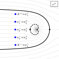
(a) $-2\pi<p<0$

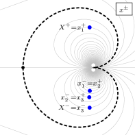
(b) $-4\pi<p<-2\pi$

Figure 20: Typical configurations corresponding to bound states with $p<0$. Figure LABEL:sub@fig:x-boundstates-min-1 shows a bound state with $m=4$ and $p\in(-2\pi,0)$ and figure LABEL:sub@fig:x-boundstates-min-2 shows a bound state with $m=2$ and $p\in(-4\pi,-2\pi)$. In figure LABEL:sub@fig:x-boundstates-min-2, note $x_{j}^{-}$ gets closer to the kidney contour with increasing $j$.

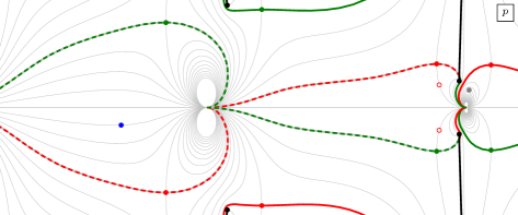
Figure 21: Two two-particle bound states. The red circles show a bound state with momentum in the $(-2\pi,0)$ range, while the dots show a bound state in the $(-4\pi,-2\pi)$ range. Note that the dot on the right, close to the origin of the $p$ plane, is drawn in grey to represent that it is located on the other sheet of the $p$ plane, and thus carries energy with a negative real part.

To construct a bound state with momentum in the range $(-2\pi,0)$, we can start with a bound state in $(0,2\pi)$ and analytically continue all Zhukovsky parameters through the scallion, essentially following the same path we would use for a single fundamental excitation. Since the log cuts through the region between the scallion and the kidney it is unavoidable that half of the Zhukovsky parameters go through the log cut. An example of such a bound state is shown in figure 20a.

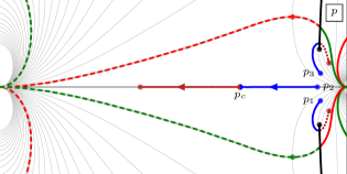
(a)

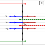
(b)

Figure 22: Three-particle bound state. Here $h=1$ and $k=7$.

In this momentum region, bound state constituents exhibit a novel property. To see this, consider a three-particle state with momentum in the range $(-2\pi,0)$ and close to 0, as shown by the blue dots in figure 22. The middle excitation has real momentum $p_{2}$ and thus real energy $E_{2}$, while the outer excitations have complex momenta $p_{1}$ and $p_{3}$ and complex energies $E_{1}$ and $E_{3}$. Since the total momentum and energy of the bound state are real, we have $p_{1}=p_{3}^{*}$ and $E_{1}=E_{3}^{*}$. Let us now make the total momentum more negative. This also decreases $p_{2}$. As $p_{2}$ hits some critical value $p_{\text{c}}$, the outer excitations hit the black line representing the cut of $E(p)$. This means that the real parts of $E_{1}$ and $E_{3}$ vanish. If we further lower the momentum, $\mathop{\mathrm{Re}}E_{1}$ and $\mathop{\mathrm{Re}}E_{3}$ will become negative. Hence, for $p_{2}<p_{\text{c}}$ we find that a single excitation with momentum $p_{2}$ has higher energy then that of the three-particle bound state we can build on top of it. We saw this behaviour earlier in the plot of the bound state dispersion relations in figure 16: at low momentum the energy decreases as the bound state number increases. This unusual non-relativistic behaviour does not lead to a pathology. If we think about the bound state dispersion relation as a function of $m$ for a fixed bound state momentum $p$, that function has a minimum at $m=-kp$, which means that the spectrum still is bounded from below.

Finally, we note that there is only $2k-1$ contours between the scallion and the kidney. Thus, only bound states with $m\leq k$ can have all their constituents in the same region. If we want to go beyond that we need to include excitations that have, e.g., $x^{-}$ inside (or on) the scallion and $x^{+}$ outside the scallion. Allowing for that we can however build bound states for any $m$.

Bound states with $p<-2\pi$.

To construct a bound state with $p\in(-4\pi,-2\pi)$ we start with a bound state in the $(-2\pi,0)$ region and continue the top component to the $(-4\pi,-2\pi)$ region. In doing so the other constituents of our starting bound state will unavoidably go into the crossed $(0,2\pi)$ region. This results in a state where all the excitations sit inside the kidney, see figure 20b. The same construction can be used to build bound states with $p<-4\pi$.

Just as for bound states in the $(-2\pi,0)$, for a given momentum region $(2\pi n,2\pi(n+1))$ with $n<-1$ there is only a finite number of states ($|n|k-1$) with all excitations inside the kidney.

2.5 “Physical” and “crossed” regions

In the pure R-R theory the Zhukovsky plane is naturally partitioned into four distinct regions. In the physical region $x^{\pm}$ sit outside the unit circle, in the crossed region they both sit inside the unit circle, and in the two mirror regions, one of $x^{+}$ or $x^{-}$ sits inside the circle and the other outside. The physical region is so called because for any physical fundamental excitation or bound state, i.e., any state with real momentum and real positive energy, we can take all the Zhukovsky parameters of the constituents to be outside the circle. Similarly, any on-shell crossed state, i.e., a state with real momentum and real negative energy, can be chosen such that all Zhukovsky parameters are inside the circle.

In the mixed-flux theory this is no longer the case. Indeed, a fundamental physical excitation with momentum in $(-2\pi,0)$ and a crossed excitation with the same momentum both sit in the region between the scallion and the kidney. Moreover, as we saw in the previous section, bound states with momentum less than $0$ in general have constituents whose energy has a negative real part.

2.6 The R representation

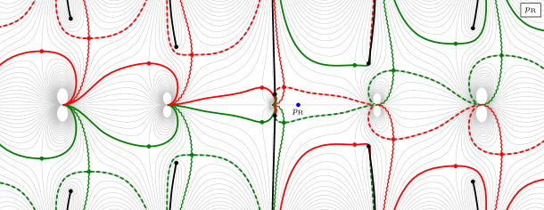
(a) The $p_{\mbox{\tiny R}}$ plane

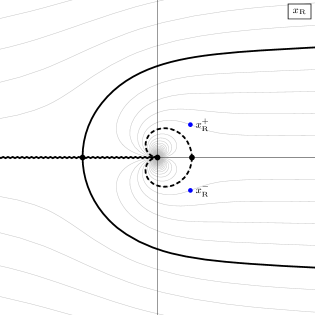
(b) The $x_{\mbox{\tiny R}}$ plane

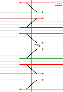
(c) The $u_{\mbox{\tiny R}}$ plane

Figure 23: The $p_{\mbox{\tiny R}}$, $x_{\mbox{\tiny R}}$ and $u_{\mbox{\tiny R}}$ planes. The blue dots show the location of a fundamental excitation with momentum $p\in(0,2\pi)$. Red (green) solid lines represent the $x_{\mbox{\tiny R}}^{+}$ ($x_{\mbox{\tiny R}}^{-}$) scallion and red (green) dashed lines represent the $x_{\mbox{\tiny R}}^{+}$ ($x_{\mbox{\tiny R}}^{-}$) kidney. The solid black lines in the $p_{\mbox{\tiny R}}$ and $u_{\mbox{\tiny R}}$ planes show the cut of the R dispersion relation. These cuts are not shown in the $x_{\mbox{\tiny R}}$ plane since they would be located at different spots for $x_{\mbox{\tiny R}}^{+}$ and $x_{\mbox{\tiny R}}^{-}$.

So far we have mainly discussed the L representation. As can be seen from the shortening condition (2.6) the R representation is essentially the parity conjugate of the L representation. Figure 23a shows the $p_{\mbox{\tiny R}}$ plane, which looks like the $p_{\mbox{\tiny L}}$ plane but reflected along the imaginary axis. In figure 23b we show the $x_{\mbox{\tiny R}}$ plane, with the same scallion and kidney cuts as in the L case, but again reflected along the imaginary axis. Note that we still put the log cut along the negative real line. The $u_{\mbox{\tiny R}}$ rapidity is defined through the function

$$u_{\mbox{\tiny R}}(x)=x+\frac{1}{x}+\frac{2\mathchar 22\relax\mkern-9.0muk}{h}\log x,\qquad u_{\mbox{\tiny R}}(x_{\mbox{\tiny R}}^{\pm})=u_{\mbox{\tiny R}}\pm\frac{i}{h}.$$ (2.29)

The $u_{\mbox{\tiny R}}$ plane is shown in figure 23c. We note that the scallion and kidney cuts in the $u_{\mbox{\tiny R}}$ plane go in the opposite direction to those of the $u_{\mbox{\tiny L}}$ plane, and that the whole plane is shifted by $ik/h$, so that the real line represents the momentum range $(0,2\pi)$, which for R excitations corresponds to the region between the scallion and the kidney in the $x_{\mbox{\tiny R}}$ plane.

3 The crossing transformation

In this section we discuss the crossing transformation in mixed-flux kinematics. Analogously to the R-R case, the mixed-flux crossing transformation sends

$$p\to\bar{p}=-p,\qquad E(p)\to\bar{E}(\bar{p})=-E(-p).$$ (3.1)

In contrast to the R-R case, the mixed-flux model is not parity invariant. In particular, the dispersion relations are not even functions of the momentum $p$, which means that the negation of the momentum in the last expression above is important. To understand how crossing acts in the Zhukovsky variables let us start at a position $x_{\mbox{\tiny L}}^{\pm}(p)=\Xi_{\mbox{\tiny L}}^{\pm}(p,1)$. Crossing takes us through the cut in the dispersion relation so after crossing we should arrive at $\bar{x}_{\mbox{\tiny L}}^{\pm}(\bar{p})=\tilde{\Xi}_{\mbox{\tiny L}}^{\pm}(\bar{p},1)$. Now we can use the relations

$$\tilde{\Xi}_{\mbox{\tiny L}}^{\pm}(p,m)=-\frac{1}{\Xi_{\mbox{\tiny L}}^{\mp}(p,m)},\qquad\Xi_{\mbox{\tiny R}}^{\pm}(p,m)=-\Xi_{\mbox{\tiny L}}^{\mp}(-p,m),$$ (3.2)

to find that $\bar{x}_{\mbox{\tiny L}}^{\pm}(\bar{p})=-1/\Xi_{\mbox{\tiny L}}^{\mp}(\bar{p},1)=1/\Xi_{\mbox{\tiny R}}^{\pm}(p,1)$ so that the crossing transformation can be expressed as

$$x_{\mbox{\tiny L}}^{\pm}(p)\to\bar{x}_{\mbox{\tiny L}}^{\pm}(\bar{p})=\frac{1}{x_{\mbox{\tiny R}}^{\pm}(p)}.$$ (3.3)

The fact that crossing an L excitation gives an R excitation can be anticipated from (2.6): $1/x_{\mbox{\tiny R}}^{\pm}(p)$ satisfy the L shortening conditions while $1/x_{\mbox{\tiny L}}^{\pm}(p)$ do not.

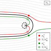
(a)

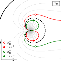
(b)

Figure 24: Location of $x_{\mbox{\tiny L}}^{\pm}(p)$, $x_{\mbox{\tiny R}}^{\pm}(p)$, $1/x_{\mbox{\tiny L}}^{\pm}(p)$, and $1/x_{\mbox{\tiny R}}^{\pm}(p)$ for real momentum in the range $0\leq p<2\pi$. Crossing of $x_{\mbox{\tiny L}}^{\pm}(p)$ is associated with going across the outer black scallion contour and crossing of $x_{\mbox{\tiny R}}^{\pm}(p)$ is associated with going across the inner black dashed kidney contour.

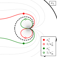
(a)

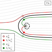
(b)

Figure 25: Location of $x_{\mbox{\tiny L}}^{\pm}(p)$, $x_{\mbox{\tiny R}}^{\pm}(p)$, $1/x_{\mbox{\tiny L}}^{\pm}(p)$, and $1/x_{\mbox{\tiny R}}^{\pm}(p)$ for real momentum in the range $-2\pi\leq p<0$. Crossing of $x_{\mbox{\tiny L}}^{\pm}(p)$ is associated with going across the inner black dashed kidney contour and crossing of $x_{\mbox{\tiny R}}^{\pm}(p)$ is associated with going across the outer black scallion contour.

Figures 24 and 25 show the points $x_{\mbox{\tiny L}}^{\pm}$ and $x_{\mbox{\tiny R}}^{\pm}$ of two physical excitations with real momentum $p$, as well as the corresponding crossed points $1/x_{\mbox{\tiny R}}^{\pm}$ and $1/x_{\mbox{\tiny L}}^{\pm}$, for momenta in the ranges $0\leq p<2\pi$ and $-2\pi\leq p<0$, respectively. These figures show that the scallion and kidney contours make up a natural border between the physical and crossed regions, for these ranges of momenta: the crossing transformation is an analytical continuation of the S matrix from outside to inside these contours.

Since the Zhukovsky and $u$ planes are made up of many sheets we need to have a convention for how to perform the analytic continuation from a physical to a crossed point. From the point of view of of the $p$ plane it is clear that we have to take a path from $p$ to $-p$ and cross one of the black $E_{I}(p)$ cuts depicted in figure 1. A priori we can cross any one of these cuts and some choices are depicted in figure 26. Depicted there are two dark blue paths labelled $1$ and $1^{\prime}$, which take a direct path between $p$ and $\bar{p}$.

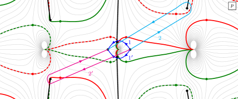
Figure 26: A few of the possible choices for crossing paths in the $p$ plane with short cuts.

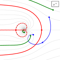
(a) $x^{+}_{\mbox{\tiny L}}$

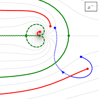
(b) $x^{-}_{\mbox{\tiny L}}$

Figure 27: Our chosen crossing path in the $x^{\pm}_{\mbox{\tiny L}}$ planes, for starting momenta $p\in[0,2\pi]$.

The image of path $1$ in Zhukovsky variables is shown in figure 27. The convention we adopt is that both $x^{+}_{\mbox{\tiny L}}$ and $x^{-}_{\mbox{\tiny L}}$ scallions are entered from the lower-half-plane.. We will adopt this path as our chosen crossing path when solving the crossing equations below. Other crossing paths such as $1^{\prime}$, or the light-blue and pink ones depicted in figure 26 as well as many others can also be chosen and they lead to the same required transformations of the Zhukovsky variables (3.3). However, their paths through the various cuts is often more complicated than our minimal choice and would lead to more complicated expressions for dressing phase solutions.

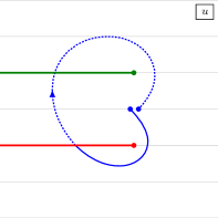
Figure 28: Our chosen crossing path in the $u_{\mbox{\tiny L}}$ plane, for starting momenta $p\in[0,2\pi]$.

Our chosen crossing path takes a simple form in the $u$ plane as depicted in figure 28. This is entirely analogous to the familiar R-R case where crossing involves going through both the $x^{+}$ and $x^{-}$ cuts a single time in the same direction. Note that, unlike the R-R case, the end-point of crossing in the $u$ plane is not the same value of $u$, because of the modified definition of the Zhukovsky map (2.10). Instead, it takes us from $u=u_{\mbox{\tiny L}}(x_{\mbox{\tiny L}}^{\pm}(p))\mp\frac{i}{h}$ to $\bar{u}=u_{\mbox{\tiny R}}(x_{\mbox{\tiny R}}^{\pm}(p))\mp\frac{i}{h}$.

4 The two-particle S matrix

As discussed in detail in [7], given two short representations of $\mathrm{psu}(1|1)^{4}_{\text{ce}}$ the two-particle S matrix is fully determined by the $\mathrm{psu}(1|1)^{4}_{\text{ce}}$ symmetry up to an overall scalar factor. If we consider only massive fundamental excitations that leaves us with four undetermined functions, which we can take as the matrix element for scattering two highest weight states

$$A_{\mathrlap{\mbox{\tiny L}\mbox{\tiny L}}\phantom{\mbox{\tiny R}\mbox{\tiny R}}}^{2}(p,q),\qquad A_{\mathrlap{\mbox{\tiny L}\mbox{\tiny R}}\phantom{\mbox{\tiny R}\mbox{\tiny R}}}^{2}(p,q),\qquad A_{\mathrlap{\mbox{\tiny R}\mbox{\tiny L}}\phantom{\mbox{\tiny R}\mbox{\tiny R}}}^{2}(p,q),\qquad A_{\mbox{\tiny R}\mbox{\tiny R}}^{2}(p,q).$$ (4.1)

These functions are further restricted by additional symmetries of the model

Physical unitarity.

The S matrix of real momentum excitation should be pure phase

$$A_{\mathrlap{\mbox{\tiny L}\mbox{\tiny L}}\phantom{\mbox{\tiny R}\mbox{\tiny R}}}^{2}(p,q)^{{\dagger}}A_{\mathrlap{\mbox{\tiny L}\mbox{\tiny L}}\phantom{\mbox{\tiny R}\mbox{\tiny R}}}^{2}(q,p) =1,\quad A_{\mathrlap{\mbox{\tiny L}\mbox{\tiny R}}\phantom{\mbox{\tiny R}\mbox{\tiny R}}}^{2}(p,q)^{{\dagger}}A_{\mathrlap{\mbox{\tiny L}\mbox{\tiny R}}\phantom{\mbox{\tiny R}\mbox{\tiny R}}}^{2}(q,p) =1,$$ (4.2)

$$A_{\mathrlap{\mbox{\tiny R}\mbox{\tiny L}}\phantom{\mbox{\tiny R}\mbox{\tiny R}}}^{2}(p,q)^{{\dagger}}A_{\mathrlap{\mbox{\tiny R}\mbox{\tiny L}}\phantom{\mbox{\tiny R}\mbox{\tiny R}}}^{2}(q,p) =1, A_{\mbox{\tiny R}\mbox{\tiny R}}^{2}(p,q)^{{\dagger}}A_{\mbox{\tiny R}\mbox{\tiny R}}^{2}(q,p) =1.$$

Braiding unitarity.

For the Zamolodchikov-Faddeev algebra to be consistent we need to impose the conditions [24]

$$A_{\mathrlap{\mbox{\tiny L}\mbox{\tiny L}}\phantom{\mbox{\tiny R}\mbox{\tiny R}}}^{2}(p,q)A_{\mathrlap{\mbox{\tiny L}\mbox{\tiny L}}\phantom{\mbox{\tiny R}\mbox{\tiny R}}}^{2}(q,p)=A_{\mathrlap{\mbox{\tiny L}\mbox{\tiny R}}\phantom{\mbox{\tiny R}\mbox{\tiny R}}}^{2}(p,q)A_{\mathrlap{\mbox{\tiny R}\mbox{\tiny L}}\phantom{\mbox{\tiny R}\mbox{\tiny R}}}^{2}(q,p)=A_{\mbox{\tiny R}\mbox{\tiny R}}^{2}(p,q)A_{\mbox{\tiny R}\mbox{\tiny R}}^{2}(q,p)=1$$ (4.3)

Parity.

The mixed-flux world-sheet theory is not parity invariant. However, a parity transformation simply swaps the L and R representations. The parity transformation acts on the Zhukovsky variables by sending $x_{\mbox{\tiny L}}^{\pm}\to-x_{\mbox{\tiny R}}^{\mp}$. From the matrix part of the S matrix we find

$$\mathbb{S}_{\mbox{\tiny R}\mbox{\tiny R}}^{t}(-p,-q)\mathbb{S}_{\mathrlap{\mbox{\tiny L}\mbox{\tiny L}}\phantom{\mbox{\tiny R}\mbox{\tiny R}}}(p,q) =A_{\mathrlap{\mbox{\tiny L}\mbox{\tiny L}}\phantom{\mbox{\tiny R}\mbox{\tiny R}}}^{2}(p,q)F_{\mbox{\tiny R}\mbox{\tiny R}}^{2}(-p,-q)\mathds{1},$$ (4.4)

$$\mathbb{S}_{\mathrlap{\mbox{\tiny R}\mbox{\tiny L}}\phantom{\mbox{\tiny R}\mbox{\tiny R}}}^{t}(-p,-q)\mathbb{S}_{\mathrlap{\mbox{\tiny L}\mbox{\tiny R}}\phantom{\mbox{\tiny R}\mbox{\tiny R}}}(p,q) =A_{\mathrlap{\mbox{\tiny L}\mbox{\tiny R}}\phantom{\mbox{\tiny R}\mbox{\tiny R}}}^{2}(p,q)F_{\mathrlap{\mbox{\tiny R}\mbox{\tiny L}}\phantom{\mbox{\tiny R}\mbox{\tiny R}}}^{2}(-p,-q)\mathds{1}.$$

From this we find the following constraints on the scalar factors

$$A_{\mbox{\tiny R}\mbox{\tiny R}}^{2}(-p,-q)A_{\mathrlap{\mbox{\tiny L}\mbox{\tiny L}}\phantom{\mbox{\tiny R}\mbox{\tiny R}}}^{2}(p,q) =\frac{x^{-}}{x^{+}}\frac{y^{+}}{y^{-}}\bigl{(}\frac{x^{+}-y^{-}}{x^{-}-y^{+}}\bigr{)}^{2},$$ (4.5)

$$A_{\mathrlap{\mbox{\tiny R}\mbox{\tiny L}}\phantom{\mbox{\tiny R}\mbox{\tiny R}}}^{2}(-p,-q)A_{\mathrlap{\mbox{\tiny L}\mbox{\tiny R}}\phantom{\mbox{\tiny R}\mbox{\tiny R}}}^{2}(p,q) =\frac{x^{+}}{x^{-}}\frac{y^{+}}{y^{-}}\bigl{(}\frac{1-\frac{1}{x^{+}y^{+}}}{1-\frac{1}{x^{-}y^{-}}}\bigr{)}^{2},$$

Crossing symmetry.

The crossing equations in the mixed-flux background were found in [7]. It is useful to write them directly in terms of S matrix elements since those equations are independent of the normalisation of the S matrix. Thus, let us define the matrix elements

$$\Upsilon^{\mathrlap{\mbox{\tiny L}\mbox{\tiny L}}\phantom{\mbox{\tiny R}\mbox{\tiny R}}}_{pq} =\braket{Y^{\mbox{\tiny L}}_{q}Y^{\mbox{\tiny L}}_{p}}{\mathcal{S}}{Y^{\mbox{\tiny L}}_{p}Y^{\mbox{\tiny L}}_{q}}=A_{\mathrlap{\mbox{\tiny L}\mbox{\tiny L}}\phantom{\mbox{\tiny R}\mbox{\tiny R}}}^{2}(p,q),\quad \Upsilon^{\mathrlap{\mbox{\tiny R}\mbox{\tiny L}}\phantom{\mbox{\tiny R}\mbox{\tiny R}}}_{pq} =\braket{Y^{\mbox{\tiny L}}_{q}Y^{\mbox{\tiny R}}_{p}}{\mathcal{S}}{Y^{\mbox{\tiny R}}_{p}Y^{\mbox{\tiny L}}_{q}}=D_{\mathrlap{\mbox{\tiny R}\mbox{\tiny L}}\phantom{\mbox{\tiny R}\mbox{\tiny R}}}^{2}(p,q),$$ (4.6)

$$\Lambda^{\mathrlap{\mbox{\tiny R}\mbox{\tiny L}}\phantom{\mbox{\tiny R}\mbox{\tiny R}}}_{pq} =\braket{Z^{\mbox{\tiny L}}_{q}Y^{\mbox{\tiny R}}_{p}}{\mathcal{S}}{Y^{\mbox{\tiny R}}_{p}Z^{\mbox{\tiny L}}_{q}}=F_{\mathrlap{\mbox{\tiny R}\mbox{\tiny L}}\phantom{\mbox{\tiny R}\mbox{\tiny R}}}^{2}(p,q),\quad \Lambda^{\mathrlap{\mbox{\tiny L}\mbox{\tiny L}}\phantom{\mbox{\tiny R}\mbox{\tiny R}}}_{pq} =\braket{Z^{\mbox{\tiny L}}_{q}Y^{\mbox{\tiny L}}_{p}}{\mathcal{S}}{Y^{\mbox{\tiny L}}_{p}Z^{\mbox{\tiny L}}_{q}}=B_{\mathrlap{\mbox{\tiny L}\mbox{\tiny L}}\phantom{\mbox{\tiny R}\mbox{\tiny R}}}^{2}(p,q).$$

The crossing equations can then be written as

$$1 =\Upsilon^{\mathrlap{\mbox{\tiny L}\mbox{\tiny L}}\phantom{\mbox{\tiny R}\mbox{\tiny R}}}_{pq}\Upsilon^{\mathrlap{\mbox{\tiny R}\mbox{\tiny L}}\phantom{\mbox{\tiny R}\mbox{\tiny R}}}_{\bar{p}q}=A_{\mathrlap{\mbox{\tiny L}\mbox{\tiny L}}\phantom{\mbox{\tiny R}\mbox{\tiny R}}}^{2}(p,q)D_{\mathrlap{\mbox{\tiny R}\mbox{\tiny L}}\phantom{\mbox{\tiny R}\mbox{\tiny R}}}^{2}(\bar{p},q)=\frac{y^{+}}{y^{-}}\Bigl{(}\frac{x^{+}-y^{-}}{x^{+}-y^{+}}\Bigr{)}^{2}A_{\mathrlap{\mbox{\tiny L}\mbox{\tiny L}}\phantom{\mbox{\tiny R}\mbox{\tiny R}}}^{2}(p,q)A_{\mathrlap{\mbox{\tiny R}\mbox{\tiny L}}\phantom{\mbox{\tiny R}\mbox{\tiny R}}}^{2}(\bar{p},q),$$ (4.7)

$$1 =\Lambda^{\mathrlap{\mbox{\tiny R}\mbox{\tiny L}}\phantom{\mbox{\tiny R}\mbox{\tiny R}}}_{pq}\Lambda^{\mathrlap{\mbox{\tiny L}\mbox{\tiny L}}\phantom{\mbox{\tiny R}\mbox{\tiny R}}}_{\bar{p}q}=F_{\mathrlap{\mbox{\tiny R}\mbox{\tiny L}}\phantom{\mbox{\tiny R}\mbox{\tiny R}}}^{2}(p,q)B_{\mathrlap{\mbox{\tiny L}\mbox{\tiny L}}\phantom{\mbox{\tiny R}\mbox{\tiny R}}}^{2}(\bar{p},q)=\frac{y^{+}}{y^{-}}\Bigl{(}\frac{\frac{1}{x^{-}}-y^{-}}{\frac{1}{x^{-}}-y^{+}}\Bigr{)}^{2}A_{\mathrlap{\mbox{\tiny R}\mbox{\tiny L}}\phantom{\mbox{\tiny R}\mbox{\tiny R}}}^{2}(p,q)A_{\mathrlap{\mbox{\tiny L}\mbox{\tiny L}}\phantom{\mbox{\tiny R}\mbox{\tiny R}}}^{2}(\bar{p},q).$$

If we perform a second crossing transformation we find the double crossing relations

$$A_{\mathrlap{\mbox{\tiny L}\mbox{\tiny L}}\phantom{\mbox{\tiny R}\mbox{\tiny R}}}^{2}(\bar{\bar{p}},q) =\Bigl{(}\frac{x^{+}-y^{-}}{x^{+}-y^{+}}\frac{x^{-}-y^{+}}{x^{-}-y^{-}}\Bigr{)}^{2}A_{\mathrlap{\mbox{\tiny L}\mbox{\tiny L}}\phantom{\mbox{\tiny R}\mbox{\tiny R}}}^{2}(p,q),$$ (4.8)

$$A_{\mathrlap{\mbox{\tiny R}\mbox{\tiny L}}\phantom{\mbox{\tiny R}\mbox{\tiny R}}}^{2}(\bar{\bar{p}},q) =\Bigl{(}\frac{\frac{1}{x^{+}}-y^{+}}{\frac{1}{x^{+}}-y^{-}}\frac{\frac{1}{x^{-}}-y^{-}}{\frac{1}{x^{-}}-y^{+}}\Bigr{)}^{2}A_{\mathrlap{\mbox{\tiny R}\mbox{\tiny L}}\phantom{\mbox{\tiny R}\mbox{\tiny R}}}^{2}(p,q).$$

Since $x_{\mbox{\tiny I}}^{\pm}(\bar{\bar{p}})=x_{\mbox{\tiny I}}^{\pm}(p)$ the double crossing equations describe non-trivial monodromies of the scalar factors.

5 The R-R scalar factors

In the R-R theory the scalar factors were chosen as [10, 29, 30]

$$A_{\mathrlap{\mbox{\tiny L}\mbox{\tiny L}}\phantom{\mbox{\tiny R}\mbox{\tiny R}}}^{2}(p,q) =\frac{x^{+}}{x^{-}}\frac{y^{-}}{y^{+}}\frac{x^{-}-y^{+}}{x^{+}-y^{-}}\frac{1-\frac{1}{x^{-}y^{+}}}{1-\frac{1}{x^{+}y^{-}}}\sigma_{\mathrlap{\mbox{\tiny L}\mbox{\tiny L}}\phantom{\mbox{\tiny R}\mbox{\tiny R}}}^{-2}(p,q),$$ (5.1)

$$A_{\mathrlap{\mbox{\tiny R}\mbox{\tiny L}}\phantom{\mbox{\tiny R}\mbox{\tiny R}}}^{2}(p,q) =\frac{x^{+}}{x^{-}}\frac{1-\frac{1}{x^{+}y^{+}}}{1-\frac{1}{x^{-}y^{-}}}\frac{1-\frac{1}{x^{-}y^{+}}}{1-\frac{1}{x^{+}y^{-}}}\sigma_{\mathrlap{\mbox{\tiny R}\mbox{\tiny L}}\phantom{\mbox{\tiny R}\mbox{\tiny R}}}^{-2}(p,q).$$

Inserting this into (4.7) we find the crossing equations for the dressing phases $\sigma_{\mbox{\tiny I}\mbox{\tiny J}}$ [27]

$$\sigma_{\mathrlap{\mbox{\tiny L}\mbox{\tiny L}}\phantom{\mbox{\tiny R}\mbox{\tiny R}}}^{2}(p,q)\sigma_{\mathrlap{\mbox{\tiny R}\mbox{\tiny L}}\phantom{\mbox{\tiny R}\mbox{\tiny R}}}^{2}(\bar{p},q) =\frac{(x^{+}-y^{-})(x^{-}-y^{+})}{(x^{+}-y^{+})(x^{-}-y^{-})}\biggl{(}\frac{y^{-}}{y^{+}}\biggr{)}^{\!\!2}\frac{x^{-}-y^{+}}{x^{+}-y^{-}}\frac{1-\frac{1}{x^{-}y^{+}}}{1-\frac{1}{x^{+}y^{-}}},$$ (5.2)

$$\sigma_{\mathrlap{\mbox{\tiny R}\mbox{\tiny L}}\phantom{\mbox{\tiny R}\mbox{\tiny R}}}^{2}(p,q)\sigma_{\mathrlap{\mbox{\tiny L}\mbox{\tiny L}}\phantom{\mbox{\tiny R}\mbox{\tiny R}}}^{2}(\bar{p},q) =\frac{\bigl{(}\frac{1}{x^{+}}-y^{+}\bigr{)}\bigl{(}\frac{1}{x^{-}}-y^{-}\bigr{)}}{\bigl{(}\frac{1}{x^{+}}-y^{-}\bigr{)}\bigl{(}\frac{1}{x^{-}}-y^{+}\bigr{)}}\biggl{(}\frac{y^{-}}{y^{+}}\biggr{)}^{\!\!2}\frac{x^{-}-y^{+}}{x^{+}-y^{-}}\frac{1-\frac{1}{x^{-}y^{+}}}{1-\frac{1}{x^{+}y^{-}}}.$$

Here we have factorised the right hand side so that the first factor corresponds to the odd crossing equation.

In reference [27] the dressing phases were written as $\sigma_{\mbox{\tiny I}\mbox{\tiny J}}^{2}(p,q)=\exp(2i\theta_{\mbox{\tiny I}\mbox{\tiny J}}(x^{\pm},y^{\pm})$ and then expanded in a chi decomposition

$$\theta_{\mbox{\tiny I}\mbox{\tiny J}}(x^{\pm},y^{\pm})=\chi_{\mbox{\tiny I}\mbox{\tiny J}}(x^{+},y^{+})-\chi_{\mbox{\tiny I}\mbox{\tiny J}}(x^{+},y^{-})-\chi_{\mbox{\tiny I}\mbox{\tiny J}}(x^{-},y^{+})+\chi_{\mbox{\tiny I}\mbox{\tiny J}}(x^{-},y^{-}).$$ (5.3)

The crossing equations were then solved by splitting the dressing phases into two parts

$$\chi_{\mathrlap{\mbox{\tiny L}\mbox{\tiny L}}\phantom{\mbox{\tiny R}\mbox{\tiny R}}}(x,y)=\chi_{\text{BES}}(x,y)+\chi^{\text{extra}}_{\mathrlap{\mbox{\tiny L}\mbox{\tiny L}}\phantom{\mbox{\tiny R}\mbox{\tiny R}}}(x,y),\qquad\chi_{\mathrlap{\mbox{\tiny R}\mbox{\tiny L}}\phantom{\mbox{\tiny R}\mbox{\tiny R}}}(x,y)=\chi_{\text{BES}}(x,y)+\chi^{\text{extra}}_{\mathrlap{\mbox{\tiny R}\mbox{\tiny L}}\phantom{\mbox{\tiny R}\mbox{\tiny R}}}(x,y),$$ (5.4)

where $\chi_{\text{BES}}$ is the BHL/BES phase [20, 22] and the extra terms can be written in terms of the HL phase $\chi_{\text{HL}}$ and a new phase $\chi_{-}$ as

$$\chi^{\text{extra}}_{\mathrlap{\mbox{\tiny L}\mbox{\tiny L}}\phantom{\mbox{\tiny R}\mbox{\tiny R}}}(x,y) =-\frac{1}{2}\chi_{\text{HL}}(x,y)+\frac{1}{2}\chi_{-}(x,y),$$ (5.5)

$$\chi^{\text{extra}}_{\mathrlap{\mbox{\tiny R}\mbox{\tiny L}}\phantom{\mbox{\tiny R}\mbox{\tiny R}}}(x,y) =-\frac{1}{2}\chi_{\text{HL}}(x,y)-\frac{1}{2}\chi_{-}(x,y).$$

Here we instead want to split the phases into the even and odd parts

$$\chi_{\mathrlap{\mbox{\tiny L}\mbox{\tiny L}}\phantom{\mbox{\tiny R}\mbox{\tiny R}}}(x,y)=\chi_{\mathrlap{\mbox{\tiny L}\mbox{\tiny L}}\phantom{\mbox{\tiny R}\mbox{\tiny R}}}^{\text{even}}(x,y)+\chi_{\mathrlap{\mbox{\tiny L}\mbox{\tiny L}}\phantom{\mbox{\tiny R}\mbox{\tiny R}}}^{\text{odd}}(x,y),\qquad\chi_{\mathrlap{\mbox{\tiny R}\mbox{\tiny L}}\phantom{\mbox{\tiny R}\mbox{\tiny R}}}(x,y)=\chi_{\mathrlap{\mbox{\tiny R}\mbox{\tiny L}}\phantom{\mbox{\tiny R}\mbox{\tiny R}}}^{\text{even}}(x,y)+\chi_{\mathrlap{\mbox{\tiny R}\mbox{\tiny L}}\phantom{\mbox{\tiny R}\mbox{\tiny R}}}^{\text{odd}}(x,y).$$ (5.6)

The even parts are given by

$$\chi_{\mathrlap{\mbox{\tiny L}\mbox{\tiny L}}\phantom{\mbox{\tiny R}\mbox{\tiny R}}}^{\text{even}}(x,y)=\chi_{\mathrlap{\mbox{\tiny R}\mbox{\tiny L}}\phantom{\mbox{\tiny R}\mbox{\tiny R}}}^{\text{even}}(x,y)=\chi_{\text{BES}}(x,y)-\chi_{\text{HL}}(x,y),$$ (5.7)

and satisfy the crossing equations

$$\sigma_{\mathrlap{\mbox{\tiny L}\mbox{\tiny L}}\phantom{\mbox{\tiny R}\mbox{\tiny R}},\text{even}}^{2}(\bar{p},q)\sigma_{\mathrlap{\mbox{\tiny R}\mbox{\tiny L}}\phantom{\mbox{\tiny R}\mbox{\tiny R}},\text{even}}^{2}(p,q) =\bigl{(}\frac{y^{-}}{y^{+}}\bigr{)}^{2}\frac{x^{-}-y^{+}}{x^{+}-y^{-}}\frac{1-\frac{1}{x^{-}y^{+}}}{1-\frac{1}{x^{+}y^{-}}},$$ (5.8)

$$\sigma_{\mathrlap{\mbox{\tiny L}\mbox{\tiny L}}\phantom{\mbox{\tiny R}\mbox{\tiny R}},\text{even}}^{2}(p,q)\sigma_{\mathrlap{\mbox{\tiny R}\mbox{\tiny L}}\phantom{\mbox{\tiny R}\mbox{\tiny R}},\text{even}}^{2}(\bar{p},q) =\bigl{(}\frac{y^{-}}{y^{+}}\bigr{)}^{2}\frac{x^{-}-y^{+}}{x^{+}-y^{-}}\frac{1-\frac{1}{x^{-}y^{+}}}{1-\frac{1}{x^{+}y^{-}}}.$$

Note that the right hand sides of these equations are invariant under $x^{\pm}\to 1/x^{\pm}$. Using these phases we can build the even matrix elements

$$A_{\mathrlap{\mbox{\tiny L}\mbox{\tiny L}}\phantom{\mbox{\tiny R}\mbox{\tiny R}},\text{even}}^{2}(p,q) =\frac{x^{+}}{x^{-}}\frac{y^{-}}{y^{+}}\frac{x^{-}-y^{+}}{x^{+}-y^{-}}\frac{1-\frac{1}{x^{-}y^{+}}}{1-\frac{1}{x^{+}y^{-}}}\sigma_{\mathrlap{\mbox{\tiny L}\mbox{\tiny L}}\phantom{\mbox{\tiny R}\mbox{\tiny R}},\text{even}}^{-2}(p,q),$$ (5.9)

$$A_{\mathrlap{\mbox{\tiny R}\mbox{\tiny L}}\phantom{\mbox{\tiny R}\mbox{\tiny R}},\text{even}}^{2}(p,q) =\frac{x^{+}}{x^{-}}\frac{y^{-}}{y^{+}}\sigma_{\mathrlap{\mbox{\tiny R}\mbox{\tiny L}}\phantom{\mbox{\tiny R}\mbox{\tiny R}},\text{even}}^{-2}(p,q),$$

which satisfy the homogenous crossing equations

$$A_{\mathrlap{\mbox{\tiny L}\mbox{\tiny L}}\phantom{\mbox{\tiny R}\mbox{\tiny R}},\text{even}}^{2}(\bar{p},q)A_{\mathrlap{\mbox{\tiny R}\mbox{\tiny L}}\phantom{\mbox{\tiny R}\mbox{\tiny R}},\text{even}}^{2}(p,q)=1,\qquad A_{\mathrlap{\mbox{\tiny L}\mbox{\tiny L}}\phantom{\mbox{\tiny R}\mbox{\tiny R}},\text{even}}^{2}(p,q)A_{\mathrlap{\mbox{\tiny R}\mbox{\tiny L}}\phantom{\mbox{\tiny R}\mbox{\tiny R}},\text{even}}^{2}(\bar{p},q)=1.$$ (5.10)

The odd matrix elements are given by

$$A_{\mathrlap{\mbox{\tiny L}\mbox{\tiny L}}\phantom{\mbox{\tiny R}\mbox{\tiny R}},\text{odd}}^{2}(p,q)=\sigma_{\mathrlap{\mbox{\tiny L}\mbox{\tiny L}}\phantom{\mbox{\tiny R}\mbox{\tiny R}},\text{odd}}^{-2}(p,q),\quad A_{\mathrlap{\mbox{\tiny R}\mbox{\tiny L}}\phantom{\mbox{\tiny R}\mbox{\tiny R}},\text{odd}}^{2}(p,q)=\frac{y^{+}}{y^{-}}\frac{1-\frac{1}{x^{+}y^{+}}}{1-\frac{1}{x^{-}y^{-}}}\frac{1-\frac{1}{x^{-}y^{+}}}{1-\frac{1}{x^{+}y^{-}}}\sigma_{\mathrlap{\mbox{\tiny R}\mbox{\tiny L}}\phantom{\mbox{\tiny R}\mbox{\tiny R}},\text{odd}}^{-2}(p,q).$$ (5.11)

Inserting these into the crossing equations we find that the odd phases should satisfy the odd crossing equation

$$\sigma_{\mathrlap{\mbox{\tiny L}\mbox{\tiny L}}\phantom{\mbox{\tiny R}\mbox{\tiny R}},\text{odd}}^{2}(\bar{p},q)\sigma_{\mathrlap{\mbox{\tiny R}\mbox{\tiny L}}\phantom{\mbox{\tiny R}\mbox{\tiny R}},\text{odd}}^{2}(p,q) =\frac{\frac{1}{x^{+}}-y^{+}}{\frac{1}{x^{+}}-y^{-}}\frac{\frac{1}{x^{-}}-y^{-}}{\frac{1}{x^{-}}-y^{+}},$$ (5.12)

$$\sigma_{\mathrlap{\mbox{\tiny L}\mbox{\tiny L}}\phantom{\mbox{\tiny R}\mbox{\tiny R}},\text{odd}}^{2}(p,q)\sigma_{\mathrlap{\mbox{\tiny R}\mbox{\tiny L}}\phantom{\mbox{\tiny R}\mbox{\tiny R}},\text{odd}}^{2}(\bar{p},q) =\frac{x^{+}-y^{-}}{x^{+}-y^{+}}\frac{x^{-}-y^{+}}{x^{-}-y^{-}}.$$

Note that the square of the right hand side of these equations are the factors appearing in the double crossing equations (4.8).

To find a solution to these equations let us start with the expression found in [27] and call the two odd phases obtained from there $\phi_{\mathrlap{\mbox{\tiny L}\mbox{\tiny L}}\phantom{\mbox{\tiny R}\mbox{\tiny R}}}$ and $\phi_{\mathrlap{\mbox{\tiny R}\mbox{\tiny L}}\phantom{\mbox{\tiny R}\mbox{\tiny R}}}$. We have

$$\phi_{\mathrlap{\mbox{\tiny L}\mbox{\tiny L}}\phantom{\mbox{\tiny R}\mbox{\tiny R}}}(x,y) =+\;{\int\negthickspace\negthickspace\negthickspace\negthinspace\negthinspace\mathrlap{\raisebox{-3.0pt}{\reflectbox{\rotatebox[origin={c}]{180.0}{$\curvearrowleft$}}}}\raisebox{3.0pt}{$\curvearrowleft$}}\,\frac{dz}{16\pi}\biggl{(}\frac{\log\frac{(y-z)^{2}}{y}}{x-z}-\frac{\log\frac{(x-z)^{2}}{x}}{y-z}\biggr{)},$$ (5.13)

$$\phi_{\mathrlap{\mbox{\tiny R}\mbox{\tiny L}}\phantom{\mbox{\tiny R}\mbox{\tiny R}}}(x,y) =-\;{\int\negthickspace\negthickspace\negthickspace\negthinspace\negthinspace\mathrlap{\raisebox{-3.0pt}{\reflectbox{\rotatebox[origin={c}]{180.0}{$\curvearrowleft$}}}}\raisebox{3.0pt}{$\curvearrowleft$}}\,\frac{dz}{16\pi}\biggl{(}\frac{\log\frac{(y-z)^{2}}{y}}{\frac{1}{x}-z}-\frac{\log\frac{(x-\frac{1}{z})^{2}}{x}}{y-z}\biggr{)},$$

where the integration is taken over the contour shown in figure 29a.

(a)

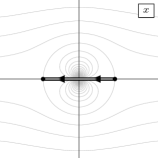
(b)

Figure 29: Integration contours for the odd R-R phases.

If we want to understand the cuts seen by $x$ it is useful to integrate by parts

$$\phi_{\mathrlap{\mbox{\tiny L}\mbox{\tiny L}}\phantom{\mbox{\tiny R}\mbox{\tiny R}}}(x,y) =+\;{\int\negthickspace\negthickspace\negthickspace\negthinspace\negthinspace\mathrlap{\raisebox{-3.0pt}{\reflectbox{\rotatebox[origin={c}]{180.0}{$\curvearrowleft$}}}}\raisebox{3.0pt}{$\curvearrowleft$}}\,\frac{dz}{8\pi}\frac{\log\frac{(y-z)^{2}}{y}}{x-z}$$ (5.14)

$$\qquad-\frac{1}{16\pi}\Bigl{(}\log\frac{(x-1)^{2}}{x}\log\frac{(y-1)^{2}}{y}+\log\frac{(x+1)^{2}}{x}\log\frac{(y+1)^{2}}{y}\Bigr{)},$$

$$\phi_{\mathrlap{\mbox{\tiny R}\mbox{\tiny L}}\phantom{\mbox{\tiny R}\mbox{\tiny R}}}(x,y) =-\;{\int\negthickspace\negthickspace\negthickspace\negthinspace\negthinspace\mathrlap{\raisebox{-3.0pt}{\reflectbox{\rotatebox[origin={c}]{180.0}{$\curvearrowleft$}}}}\raisebox{3.0pt}{$\curvearrowleft$}}\,\frac{dz}{8\pi}\frac{\log\frac{(y-z)^{2}}{y}}{\frac{1}{x}-z}$$

$$\qquad+\frac{1}{16\pi}\Bigl{(}\log\frac{(x-1)^{2}}{x}\log\frac{(y-1)^{2}}{y}-\log\frac{(x+1)^{2}}{x}\log\frac{(y+1)^{2}}{y}\Bigr{)}$$

We expect the phases to have cuts along the unit circle, which we indeed do get from the above expressions. However, the boundary terms have an additional unwanted log cut along the negative real lines in both the $x$ and $y$ planes and the integral term also has such a log cut in the $y$ plane. To get of rid of these we can add an extra anti-symmetric term

$$\delta\phi(x,y)=\frac{1}{16\pi}\log\frac{(x+1)^{2}}{x}\log\frac{(y-1)^{2}}{y}-\frac{1}{16\pi}\log\frac{(x-1)^{2}}{x}\log\frac{(y+1)^{2}}{y}.$$ (5.15)

The full phases $\chi_{\mathrlap{\mbox{\tiny L}\mbox{\tiny L}}\phantom{\mbox{\tiny R}\mbox{\tiny R}}}(x,y)=\phi_{\mathrlap{\mbox{\tiny L}\mbox{\tiny L}}\phantom{\mbox{\tiny R}\mbox{\tiny R}}}(x,y)+\delta\phi(x,y)$ and $\chi_{\mathrlap{\mbox{\tiny R}\mbox{\tiny L}}\phantom{\mbox{\tiny R}\mbox{\tiny R}}}(x,y)=\phi_{\mathrlap{\mbox{\tiny R}\mbox{\tiny L}}\phantom{\mbox{\tiny R}\mbox{\tiny R}}}(x,y)-\delta\phi(x,y)$ then take the form

$$\chi_{\mathrlap{\mbox{\tiny L}\mbox{\tiny L}}\phantom{\mbox{\tiny R}\mbox{\tiny R}}}(x,y) =+\;{\int\negthickspace\negthickspace\negthickspace\negthinspace\negthinspace\mathrlap{\raisebox{-3.0pt}{\reflectbox{\rotatebox[origin={c}]{180.0}{$\curvearrowleft$}}}}\raisebox{3.0pt}{$\curvearrowleft$}}\,\frac{dz}{8\pi}\frac{\log\frac{(y-z)^{2}}{y}}{x-z}+\frac{1}{16\pi}\log\frac{(x+1)^{2}}{(x-1)^{2}}\Bigl{(}\log\frac{(y+1)^{2}}{y}+\log\frac{(y-1)^{2}}{y}\Bigr{)},$$ (5.16)

$$\chi_{\mathrlap{\mbox{\tiny R}\mbox{\tiny L}}\phantom{\mbox{\tiny R}\mbox{\tiny R}}}(x,y) =-\;{\int\negthickspace\negthickspace\negthickspace\negthinspace\negthinspace\mathrlap{\raisebox{-3.0pt}{\reflectbox{\rotatebox[origin={c}]{180.0}{$\curvearrowleft$}}}}\raisebox{3.0pt}{$\curvearrowleft$}}\,\frac{dz}{8\pi}\frac{\log\frac{(y-z)^{2}}{y}}{\frac{1}{x}-z}-\frac{1}{16\pi}\log\frac{(x+1)^{2}}{(x-1)^{2}}\Bigl{(}\log\frac{(y+1)^{2}}{y}+\log\frac{(y-1)^{2}}{y}\Bigr{)}.$$

This modification of the phase of [27] was originally proposed by Andrea Cavaglià and Simon Ekhammar [31] and leaves the crossing equation satisfied by the full phase $\theta_{\mathrlap{\mbox{\tiny L}\mbox{\tiny L}}\phantom{\mbox{\tiny R}\mbox{\tiny R}}}$ unchanged. It is possible to show that [32] this simple modification of [27] reproduces the more involved expressions given by [19], which were in turn found by generalising the expressions for massless dressing factors given in [33]. It is easy to verify that the branch points of the S matrix are not of square-root type, in line with the key finding of [27]. The analysis [28] of Dorey-Hofman-Maldacena (DHM) double-poles also remains unchanged by the addition of $\delta\phi$.

We find it useful to bring the cuts down from the unit circle to the interval $[-1,1]$. If $x$ and $y$ are outside the unit circle the LL phase remains unchanged

$$\chi_{\mathrlap{\mbox{\tiny L}\mbox{\tiny L}}\phantom{\mbox{\tiny R}\mbox{\tiny R}}}(x,y)=+\int_{1}^{-1}\frac{dz}{2\pi}\frac{\log(y-z)}{x-z}+\frac{1}{4\pi}\log\frac{x+1}{x-1}\Bigl{(}\log(y+1)+\log(y-1)\Bigr{)}.$$ (5.17)

However, when we deform the integration contour in the RL phase from the two half circles in figure 29a to the interval in figure 29b we pick up a pole at $1/x$ whose residue depends on which half-plane $x$ sits in

$$\chi_{\mathrlap{\mbox{\tiny R}\mbox{\tiny L}}\phantom{\mbox{\tiny R}\mbox{\tiny R}}}(x,y) =-\int_{1}^{-1}\frac{dz}{2\pi}\frac{\log(y-z)}{\frac{1}{x}-z}-\frac{1}{4\pi}\log\frac{x+1}{x-1}\Bigl{(}\log(y+1)+\log(y-1)\Bigr{)}$$ (5.18)

$$\qquad-\frac{i}{2}\operatorname{sign}(\mathop{\mathrm{Im}}x)\log\bigl{(}y-\frac{1}{x}\bigr{)}.$$

Note that the integral in the RL phase gives long cuts along $(-\infty,-1]\cup[1,\infty)$, but the expression in the second line exactly cancels these discontinuities so that the full expression has a cut only along the short interval $[-1,1]$.

Using the above expression we can check the crossing equations. Going through the cut from below the phases pick up additional terms

$$\delta_{\uparrow}\phi_{\mathrlap{\mbox{\tiny L}\mbox{\tiny L}}\phantom{\mbox{\tiny R}\mbox{\tiny R}}}(x,y) =-i\log(y-x)+\frac{i}{2}\bigl{(}\log(y+1)+\log(y-1)\bigr{)},$$ (5.19)

$$\delta_{\uparrow}\phi_{\mathrlap{\mbox{\tiny R}\mbox{\tiny L}}\phantom{\mbox{\tiny R}\mbox{\tiny R}}}(x,y) =+i\log\bigl{(}y-\frac{1}{x}\bigr{)}-\frac{i}{2}\bigl{(}\log(y+1)+\log(y-1)\bigr{)}.$$

Combining this with the results of [27] we find

$$\chi_{\mathrlap{\mbox{\tiny L}\mbox{\tiny L}}\phantom{\mbox{\tiny R}\mbox{\tiny R}}}\bigl{(}\frac{1}{x},y\bigr{)}+\chi_{\mathrlap{\mbox{\tiny R}\mbox{\tiny L}}\phantom{\mbox{\tiny R}\mbox{\tiny R}}}(x,y) =-\frac{i}{2}\log\bigl{(}y-\frac{1}{x}\bigr{)}+\frac{i}{4}\bigl{(}\log(y+1)+\log(y-1)\bigr{)},$$ (5.20)

$$\chi_{\mathrlap{\mbox{\tiny L}\mbox{\tiny L}}\phantom{\mbox{\tiny R}\mbox{\tiny R}}}(x,y)+\chi_{\mathrlap{\mbox{\tiny R}\mbox{\tiny L}}\phantom{\mbox{\tiny R}\mbox{\tiny R}}}\bigl{(}\frac{1}{x},y\bigr{)} =+\frac{i}{2}\log(y-x)-\frac{i}{4}\bigl{(}\log(y+1)+\log(y-1)\bigr{)}.$$

The last term on each line cancels out in the full dressing phase (5.3).

Before ending this section let us consider the poles of the R-R S matrix. We have split the R-R matrix elements into two parts. The odd part transforms non-trivially under crossing, but does not have any singularities in the physical or crossed regions. This is easy to see for the LL phase: neither the rational pre-factor nor the phase has any relevant poles. For the RL case we note that for excitations with real momenta (so that $x^{+}$ and $x^{-}$ is in the upper and lower half-planes respectively) the term on the last line in equation (5.18) exactly cancels the rational factor in $A_{\mathrlap{\mbox{\tiny R}\mbox{\tiny L}}\phantom{\mbox{\tiny R}\mbox{\tiny R}},\text{odd}}^{2}$. The even parts of the matrix elements, on the other hand, are trivial under crossing but responsible for all physically relevant poles. We could thus think of it as a CDD factor [34], though in general we expect it to have an intricate analytic structure. In $A_{\mathrlap{\mbox{\tiny L}\mbox{\tiny L}}\phantom{\mbox{\tiny R}\mbox{\tiny R}},\text{even}}^{2}$ in (5.10) we directly find an S channel zero at $x^{-}=y^{+}$ which corresponds to the formation of a bound state. The even phase has a pole at $x^{-}=1/y^{+}$ which cancels the zero in $A_{\mathrlap{\mbox{\tiny L}\mbox{\tiny L}}\phantom{\mbox{\tiny R}\mbox{\tiny R}},\text{even}}^{2}$ and provides us with the expected T channel pole in $A_{\mathrlap{\mbox{\tiny R}\mbox{\tiny L}}\phantom{\mbox{\tiny R}\mbox{\tiny R}},\text{even}}^{2}$. Finally the BES part of the phase gives rise to DHM double poles corresponding to the formation of an on-shell bound state in an intermediate channel [35, 28].

6 The mixed-flux scalar factors

In this section we will construct the scalar factors in the mixed-flux theory. As in the pure R-R theory, we split the scalar factors into odd and even parts (5.6).

6.1 The odd scalar factor

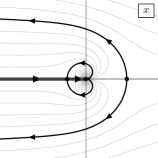
(a)

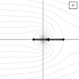
(b)

Figure 30: Mixed-flux integration contours

For the odd scalar factor we start with the odd matrix elements which are similar to the odd R-R matrix elements

$$A_{\mathrlap{\mbox{\tiny L}\mbox{\tiny L}}\phantom{\mbox{\tiny R}\mbox{\tiny R}},\text{odd}}^{2}(p,q) =\Bigl{(}\frac{\alpha(x^{-})\alpha(y^{+})}{\alpha(x^{+})\alpha(y^{-})}\Bigr{)}^{\!\!1/k}\sigma_{\mathrlap{\mbox{\tiny L}\mbox{\tiny L}}\phantom{\mbox{\tiny R}\mbox{\tiny R}},\text{odd}}^{-2}(p,q),$$ (6.1)

$$A_{\mathrlap{\mbox{\tiny R}\mbox{\tiny L}}\phantom{\mbox{\tiny R}\mbox{\tiny R}},\text{odd}}^{2}(p,q) =\Bigl{(}\frac{\alpha(1/x^{+})\alpha(y^{-})}{\alpha(1/x^{-})\alpha(y^{+})}\Bigr{)}^{\!\!1/k}\frac{y^{+}}{y^{-}}\frac{1-\frac{1}{x^{+}y^{+}}}{1-\frac{1}{x^{-}y^{-}}}\frac{1-\frac{1}{x^{-}y^{+}}}{1-\frac{1}{x^{+}y^{-}}}\sigma_{\mathrlap{\mbox{\tiny R}\mbox{\tiny L}}\phantom{\mbox{\tiny R}\mbox{\tiny R}},\text{odd}}^{-2}(p,q),$$

where

$$\alpha(x)=(x-s)\Bigl{(}\frac{1}{x}+s\Bigr{)}.$$ (6.2)

The additional factors in (6.1) compared to the R-R case (5.11) trivially cancel in the crossing equations. As we discuss in section 7.2 below, these terms play an important role in fusion. The generalisation of the R-R odd phases presented in the previous section to the mixed-flux case is

$$\chi_{\mathrlap{\mbox{\tiny L}\mbox{\tiny L}}\phantom{\mbox{\tiny R}\mbox{\tiny R}}}(x,y) =+\!\!\int_{s}^{-s^{-1}}\frac{dz}{2\pi}\frac{\log(y-z)}{x-z}+\frac{1}{4\pi}\log\frac{x+s^{-1}}{\!x-s}\Bigl{(}\log(y+s^{-1})+\log(y-s)\Bigr{)},$$ (6.3)

$$\chi_{\mathrlap{\mbox{\tiny R}\mbox{\tiny L}}\phantom{\mbox{\tiny R}\mbox{\tiny R}}}(x,y) =-\!\!\int_{s}^{-s^{-1}}\frac{dz}{2\pi}\frac{\log(y-z)}{\frac{1}{x}-z}-\frac{1}{4\pi}\log\frac{\!x+s}{x-s^{-1}}\Bigl{(}\log(y+s^{-1})+\log(y-s)\Bigr{)}$$

$$\qquad-\frac{i}{2}\operatorname{sign}(\mathop{\mathrm{Im}}x)\log\bigl{(}y-\frac{1}{x}\bigr{)}.$$

The integrals are taken over the interval $[-1/s,s]$ as shown in figure 30b. It is simple to check that these phases satisfy the same crossing equations as in the pure R-R case

$$\sigma_{\mathrlap{\mbox{\tiny L}\mbox{\tiny L}}\phantom{\mbox{\tiny R}\mbox{\tiny R}},\text{odd}}^{2}(\bar{p},q)\sigma_{\mathrlap{\mbox{\tiny R}\mbox{\tiny L}}\phantom{\mbox{\tiny R}\mbox{\tiny R}},\text{odd}}^{2}(p,q) =\frac{\frac{1}{x^{+}}-y^{+}}{\frac{1}{x^{+}}-y^{-}}\frac{\frac{1}{x^{-}}-y^{-}}{\frac{1}{x^{-}}-y^{+}},$$ (6.4)

$$\sigma_{\mathrlap{\mbox{\tiny L}\mbox{\tiny L}}\phantom{\mbox{\tiny R}\mbox{\tiny R}},\text{odd}}^{2}(p,q)\sigma_{\mathrlap{\mbox{\tiny R}\mbox{\tiny L}}\phantom{\mbox{\tiny R}\mbox{\tiny R}},\text{odd}}^{2}(\bar{p},q) =\frac{x^{+}-y^{-}}{x^{+}-y^{+}}\frac{x^{-}-y^{+}}{x^{-}-y^{-}}.$$

The above integrals over $[-1/s,s]$ are useful in checking the crossing equation. It is sometimes also useful to do an integration by parts on half of the integrands above to find

$$\chi_{\mathrlap{\mbox{\tiny L}\mbox{\tiny L}}\phantom{\mbox{\tiny R}\mbox{\tiny R}}}(x,y) =+\!\!\int_{s}^{-s^{-1}}\frac{dz}{4\pi}\left[\frac{\log(y-z)}{x-z}-\frac{\log(x-z)}{y-z}\right]$$ (6.5)

$$\qquad+\frac{1}{4\pi}\left[\log(x+s^{-1})\log(y-s)-\log(x-s)\log(y+s^{-1})\right],$$

$$\chi_{\mathrlap{\mbox{\tiny R}\mbox{\tiny L}}\phantom{\mbox{\tiny R}\mbox{\tiny R}}}(x,y) =-\!\!\int_{s}^{-s^{-1}}\frac{dz}{4\pi}\frac{\log(y-z)}{\frac{1}{x}-z}+\!\!\int_{s^{-1}}^{-s}\frac{dz}{4\pi}\frac{\log(x-z)}{\frac{1}{y}-z}$$

$$\qquad-\frac{1}{4\pi}\left[\log(x+s)\log(y-s)-\log(x-s^{-1})\log(y+s^{-1})\right],$$

$$\qquad-\frac{i}{4}\operatorname{sign}(\mathop{\mathrm{Im}}x)\log\bigl{(}y-\frac{1}{x}\bigr{)}+\frac{i}{4}\operatorname{sign}(\mathop{\mathrm{Im}}y)\log\bigl{(}x-\frac{1}{y}\bigr{)}$$

As we discussed in section 3, the scallion and kidney contours are natural boundaries when considering crossing. It is therefore natural to deform $[-1/s,s]$ into scallion and kidney contours, analogously to what is depicted in figure 29 for the R-R case. Notice that the integral over $[-1/s,s]$ has no monodromy around infinity. To preserve this property after deforming the integration contour to a scallion and kidney (for non-quadratic cuts), it is necessary to introduce additional integrals over $(-\infty,0]$. The deformed contour is shown in figure 30a and the mixed-flux expressions for $\chi_{\mathrlap{\mbox{\tiny L}\mbox{\tiny L}}\phantom{\mbox{\tiny R}\mbox{\tiny R}}}$ and $\chi_{\mathrlap{\mbox{\tiny R}\mbox{\tiny L}}\phantom{\mbox{\tiny R}\mbox{\tiny R}}}$ take the same form as in (6.5), but with the following replacement of integrals

$$\int_{s}^{-s^{-1}}\longrightarrow\int_{\mathcal{I}_{L}}+2\!\!\int_{-\infty}^{0},\qquad\int_{s^{-1}}^{-s}\longrightarrow\int_{\mathcal{I}_{R}}+2\!\int_{0}^{\infty}$$ (6.6)

where the contours $\mathcal{I}_{L}$ and $\mathcal{I}_{R}$ are defined as

$$\mathcal{I}_{L}=S_{L}^{+}-S_{L}^{-}+K_{L}^{+}-K_{L}^{-},\qquad\mathcal{I}_{R}=S_{R}^{+}-S_{R}^{-}+K_{R}^{+}-K_{R}^{-},$$ (6.7)

with $K_{L}^{+}$ and $K_{L}^{-}$ the upper and lower halves of the L kidney contour traversed in an anti-clockwise direction, and similarly $S_{L}^{+}$ and $S_{L}^{-}$ for the L scallion, $K_{R}^{+}$ and $K_{R}^{-}$ for the R kidney and $S_{R}^{+}$ and $S_{R}^{-}$ for the R scallion.

It will sometimes be useful to do a “complete” integration by parts for $\chi_{\mathrlap{\mbox{\tiny R}\mbox{\tiny L}}\phantom{\mbox{\tiny R}\mbox{\tiny R}}}(x,y)$ to make its analytic structure in the $y$-plane clear

$$\chi_{\mathrlap{\mbox{\tiny R}\mbox{\tiny L}}\phantom{\mbox{\tiny R}\mbox{\tiny R}}}(x,y) =+\!\!\int_{s^{-1}}^{-s}\frac{dz}{2\pi}\frac{\log(x-z)}{\frac{1}{y}-z}+\frac{1}{4\pi}\log\frac{\!y+s^{-1}}{y-s}\Bigl{(}\log(x+s)+\log(x-s^{-1})\Bigr{)}$$ (6.8)

$$\qquad+\frac{i}{2}\operatorname{sign}(\mathop{\mathrm{Im}}y)\log\bigl{(}x-\frac{1}{y}\bigr{)}.$$

The analogous expression for the LL phase follows trivially from the anti-symmetry of $\chi_{\mathrlap{\mbox{\tiny L}\mbox{\tiny L}}\phantom{\mbox{\tiny R}\mbox{\tiny R}}}$, $\chi_{\mathrlap{\mbox{\tiny L}\mbox{\tiny L}}\phantom{\mbox{\tiny R}\mbox{\tiny R}}}(x,y)=-\chi_{\mathrlap{\mbox{\tiny L}\mbox{\tiny L}}\phantom{\mbox{\tiny R}\mbox{\tiny R}}}(y,x)$.

The expressions presented in this sub-section for $\chi_{\mathrlap{\mbox{\tiny L}\mbox{\tiny L}}\phantom{\mbox{\tiny R}\mbox{\tiny R}}}$ and $\chi_{\mathrlap{\mbox{\tiny R}\mbox{\tiny L}}\phantom{\mbox{\tiny R}\mbox{\tiny R}}}$ are valid for momenta in the region outside the left and right kidneys, i.e. for $p_{\mbox{\tiny L}}\in(0,2\pi)$ and $p_{\mbox{\tiny R}}\in(-2\pi,0)$. These regions shares many similarities with with the physical region of the R-R theory, which is outside the unit disc. In particular, it is useful to expand the dressing phases at large values of the Zhukovsky parameters. Expanding the integrand in the expression for $\chi_{\mathrlap{\mbox{\tiny L}\mbox{\tiny L}}\phantom{\mbox{\tiny R}\mbox{\tiny R}}}$ in (6.4) and then integrating gives

$$\chi_{\mathrlap{\mbox{\tiny L}\mbox{\tiny L}}\phantom{\mbox{\tiny R}\mbox{\tiny R}}}=\frac{1}{4\pi}\sum_{m,n=1}^{\infty}\frac{x^{-m}y^{-n}}{mn}\biggl{[}\frac{m-n}{m+n}\bigl{(}s^{n+m}-(-s^{-1})^{n+m}\bigr{)}+(-1)^{m}s^{n-m}-(-1)^{n}s^{m-n}\biggr{]}.$$ (6.9)

In the case of $\chi_{\mathrlap{\mbox{\tiny R}\mbox{\tiny L}}\phantom{\mbox{\tiny R}\mbox{\tiny R}}}$, it is helpful to deform the integration contour in (6.4) to two semi-circles, similar to those in the R-R case shown in figure 29a, but now going between $z=s$ and $z=-s^{-1}$. These semi-circles appeared in [25] and are useful here, because they remove the term proportional to $\operatorname{sign}(\mathop{\mathrm{Im}}x)$ After this contour deformation, it is again straightforward to expand the integrand at large values of the Zhukovsky parameters and the integrate to get

$$\chi_{\mathrlap{\mbox{\tiny R}\mbox{\tiny L}}\phantom{\mbox{\tiny R}\mbox{\tiny R}}} =\frac{\log s}{\pi}\sum_{n=1}^{\infty}\frac{1}{n}y^{-n}x^{-n}+\frac{1}{4\pi}\sum_{n=1}^{\infty}\frac{(-1)^{n}\bigl{(}s^{-2n}-s^{2n}\bigr{)}}{n^{2}}y^{-n}x^{-n}$$ (6.10)

$$\quad+\frac{1}{4\pi}\sum_{\begin{subarray}{c}m,n=1\\ m\neq n\end{subarray}}^{\infty}\frac{x^{-m}y^{-n}}{mn}\biggl{[}\frac{n+m}{n-m}\bigl{(}s^{n-m}-(-s)^{m-n}\bigr{)}+(-1)^{n}s^{-n-m}-(-1)^{m}s^{n+m}\biggr{]}$$

$$\quad-\frac{\log s}{\pi}\log y+\frac{1}{2\pi}\sum_{n=1}^{\infty}\frac{s^{n}-(-s)^{-n}}{n^{2}}y^{-n}\,,$$

where the terms on the last line can be dropped, since they are $x$-independent and so cancel out in the expression for $\theta_{\mathrlap{\mbox{\tiny R}\mbox{\tiny L}}\phantom{\mbox{\tiny R}\mbox{\tiny R}}}$.

6.2 The even scalar factor

As in the R-R case the even scalar factors satisfy the homogeneous crossing equations but provide us with physical poles and zeros. We expect the LL S matrix to have a simple pole corresponding to the formation of a bound state as discussed in section 2.4. This can be accommodated by a simple rational factor as in the pure R-R case. However, after a proper analytical continuation we also expect to find double poles corresponding to the exchange of an on-shell bound state [35, 28]. In the R-R case the double poles were provided by the BES phase, and in the mixed-flux case it seems natural to expect a generalisation of this phase to appear.

A new feature of the mixed-flux theory is the appearance of an infinite number of momentum regions $(2\pi n,2\pi(n+1))$. Here we will discuss what poles the fundamental S matrix is expected to have in different regions, and what constraints that gives for the even dressing phases.

6.2.1 Scalar factors in the $(0,2\pi)$ region

Let us start by considering the case of two fundamental excitations with momenta in $(0,2\pi)$. Here we take the even matrix element to be the same as in the R-R model (see equation (5.9)), when expressed in terms of the rapidity $u_{\mbox{\tiny L}}$

$$\begin{gathered}A_{\mathrlap{\mbox{\tiny L}\mbox{\tiny L}}\phantom{\mbox{\tiny R}\mbox{\tiny R}},\text{even}}^{2}(p,q)=\frac{x^{+}}{x^{-}}\frac{y^{-}}{y^{+}}\frac{u_{\mbox{\tiny L}}(x^{-})-u_{\mbox{\tiny L}}(y^{+})}{u_{\mbox{\tiny L}}(x^{+})-u_{\mbox{\tiny L}}(y^{-})}\sigma_{\mathrlap{\mbox{\tiny L}\mbox{\tiny L}}\phantom{\mbox{\tiny R}\mbox{\tiny R}},\text{even}}^{-2}(p,q),\\ A_{\mathrlap{\mbox{\tiny R}\mbox{\tiny L}}\phantom{\mbox{\tiny R}\mbox{\tiny R}},\text{even}}^{2}(p,q)=\frac{x^{+}}{x^{-}}\frac{y^{-}}{y^{+}}\sigma_{\mathrlap{\mbox{\tiny R}\mbox{\tiny L}}\phantom{\mbox{\tiny R}\mbox{\tiny R}},\text{even}}^{-2}(p,q).\end{gathered}$$ (6.11)

The even dressing phases satisfy the crossing equations (cf. (5.8))

$$\sigma_{\mathrlap{\mbox{\tiny L}\mbox{\tiny L}}\phantom{\mbox{\tiny R}\mbox{\tiny R}},\text{even}}^{2}(\bar{p},q)\sigma_{\mathrlap{\mbox{\tiny R}\mbox{\tiny L}}\phantom{\mbox{\tiny R}\mbox{\tiny R}},\text{even}}^{2}(p,q) =\bigl{(}\frac{y^{-}}{y^{+}}\bigr{)}^{2}\frac{u_{\mbox{\tiny L}}(x^{-})-u_{\mbox{\tiny L}}(y^{+})}{u_{\mbox{\tiny L}}(x^{+})-u_{\mbox{\tiny L}}(y^{-})},$$ (6.12)

$$\sigma_{\mathrlap{\mbox{\tiny L}\mbox{\tiny L}}\phantom{\mbox{\tiny R}\mbox{\tiny R}},\text{even}}^{2}(p,q)\sigma_{\mathrlap{\mbox{\tiny R}\mbox{\tiny L}}\phantom{\mbox{\tiny R}\mbox{\tiny R}},\text{even}}^{2}(\bar{p},q) =\bigl{(}\frac{y^{-}}{y^{+}}\bigr{)}^{2}\frac{u_{\mbox{\tiny R}}(x^{-})-u_{\mbox{\tiny L}}(y^{+})}{u_{\mbox{\tiny R}}(x^{+})-u_{\mbox{\tiny L}}(y^{-})}.$$

The LL factor has the expected S channel zero at $x^{+}=y^{-}$, and as in the R-R case we expect the even dressing phase to cancel any other relevant zero or pole in $A_{\mathrlap{\mbox{\tiny L}\mbox{\tiny L}}\phantom{\mbox{\tiny R}\mbox{\tiny R}},\text{even}}^{2}(p,q)$ and to provide us with the T channel pole of $A_{\mathrlap{\mbox{\tiny R}\mbox{\tiny L}}\phantom{\mbox{\tiny R}\mbox{\tiny R}},\text{even}}^{2}(p,q)$.

6.2.2 Scalar factors in the $(2\pi,4\pi)$ region

Consider bringing $x^{\pm}$ into the $(2\pi,4\pi)$ region. The Beisert-Dippel-Staudacher (BDS) factor [36] in (6.11) is clearly analytic as a function of $u_{\mbox{\tiny L}}$ and thus does not change when we go to a different momentum region. However, let us consider the poles and zeros we expect in the LL S matrix. As above we expect a zero when $x^{-}=y^{+}$ and a pole when $x^{+}=y^{-}$, but the analytic continuation has taken us to a different sheet of the $u_{\mbox{\tiny L}}$ plane. If we follow a path where $x^{+}$ goes around the origin we then find that the LL matrix element should be given by

$$A_{\mathrlap{\mbox{\tiny L}\mbox{\tiny L}}\phantom{\mbox{\tiny R}\mbox{\tiny R}},\text{even}}^{2}(p,q)=\frac{x^{+}}{x^{-}}\frac{y^{-}}{y^{+}}\frac{u_{\mbox{\tiny L}}(x^{-})-u_{\mbox{\tiny L}}(y^{+})}{u_{\mbox{\tiny L}}(x^{+})-u_{\mbox{\tiny L}}(y^{-})+\frac{2ik}{h}}\,\sigma_{\mathrlap{\mbox{\tiny L}\mbox{\tiny L}}\phantom{\mbox{\tiny R}\mbox{\tiny R}},\text{even}}^{-2}(p,q).$$ (6.13)

If we instead take both $x^{\pm}$ and $y^{\pm}$ to be in the $(2\pi,4\pi)$ region we instead expect

$$A_{\mathrlap{\mbox{\tiny L}\mbox{\tiny L}}\phantom{\mbox{\tiny R}\mbox{\tiny R}},\text{even}}^{2}(p,q)=\frac{x^{+}}{x^{-}}\frac{y^{-}}{y^{+}}\frac{u_{\mbox{\tiny L}}(x^{-})-u_{\mbox{\tiny L}}(y^{+})-\frac{2ik}{h}}{u_{\mbox{\tiny L}}(x^{+})-u_{\mbox{\tiny L}}(y^{-})+\frac{2ik}{h}}\,\sigma_{\mathrlap{\mbox{\tiny L}\mbox{\tiny L}}\phantom{\mbox{\tiny R}\mbox{\tiny R}},\text{even}}^{-2}(p,q).$$ (6.14)

Both of these expressions indicate that we should pick up a factor from the dressing phase when we change momentum region. In particular when we take $p$ to $p+2\pi$ with $p$ and $q$ in $(0,2\pi)$ we should pick up a factor

$$\frac{u_{\mbox{\tiny L}}(x^{+})-u_{\mbox{\tiny L}}(y^{-})}{u_{\mbox{\tiny L}}(x^{+})-u_{\mbox{\tiny L}}(y^{-})+\frac{2ik}{h}}$$ (6.15)

when we go into the scallion contour from below and exit it on the top.

6.2.3 Scalar factor for $p_{\mbox{\tiny L}}$ in $(-2\pi,0)$

In the $(-2\pi,0)$ region we have seen that the $u_{\mbox{\tiny L}}$ plane is periodic with period $2ik/h$, and we expect the S matrix to respect this. To accommodate this we propose that in this region the scalar factor takes the form

$$A_{\mathrlap{\mbox{\tiny L}\mbox{\tiny L}}\phantom{\mbox{\tiny R}\mbox{\tiny R}},\text{even}}^{2}(p,q)=\frac{\sinh\bigl{(}\frac{\pi h}{2k}\bigl{(}u_{\mbox{\tiny L}}(x^{-})-u_{\mbox{\tiny L}}(y^{+})\bigr{)}\bigr{)}}{\sinh\bigl{(}\frac{\pi h}{2k}\bigl{(}u_{\mbox{\tiny L}}(x^{+})-u_{\mbox{\tiny L}}(y^{-})\bigr{)}\bigr{)}}\sigma_{\mathrlap{\mbox{\tiny L}\mbox{\tiny L}}\phantom{\mbox{\tiny R}\mbox{\tiny R}},\text{even}}^{-2}(p,q).$$ (6.16)

Note that up to the dressing factor this is the S matrix for the XXZ model at a root of unity, i.e., with anisotropy of the form $\Delta=\cos\frac{\pi}{k}$ with $k$ an integer [37, 38, 39]. To see this more explicitly we introduce the rapidities $u$ and $v$ such that

$$u_{\mbox{\tiny L}}(x^{\pm})=u\pm\frac{i}{h},\qquad u_{\mbox{\tiny L}}(y^{\pm})=v\pm\frac{i}{h},$$ (6.17)

which gives

$$A_{\mathrlap{\mbox{\tiny L}\mbox{\tiny L}}\phantom{\mbox{\tiny R}\mbox{\tiny R}},\text{even}}^{2}(p,q)=\frac{\sinh\bigl{(}\frac{\pi h}{2k}\bigl{(}u-v-\frac{2i}{h}\bigr{)}\bigr{)}}{\sinh\bigl{(}\frac{\pi h}{2k}\bigl{(}u-v+\frac{2i}{h}\bigr{)}\bigr{)}}\sigma_{\mathrlap{\mbox{\tiny L}\mbox{\tiny L}}\phantom{\mbox{\tiny R}\mbox{\tiny R}},\text{even}}^{-2}(p,q).$$ (6.18)

The above factor provides us with the expected poles and zeros at $x^{\pm}=y^{\mp}$. For the even RL matrix element with the L excitation in $(-2\pi,0)$ and the R excitation in $(0,2\pi)$, i.e., with both excitation between respective scallion and kidney, we take

$$A_{\mathrlap{\mbox{\tiny R}\mbox{\tiny L}}\phantom{\mbox{\tiny R}\mbox{\tiny R}},\text{even}}^{2}(p,q)=\frac{\sinh\bigl{(}\frac{\pi h}{2k}\bigl{(}u_{\mbox{\tiny R}}(x^{+})-u_{\mbox{\tiny L}}(y^{-})\bigr{)}\bigr{)}}{\sinh\bigl{(}\frac{\pi h}{2k}\bigl{(}u_{\mbox{\tiny R}}(x^{-})-u_{\mbox{\tiny L}}(y^{+})\bigr{)}\bigr{)}}\sigma_{\mathrlap{\mbox{\tiny R}\mbox{\tiny L}}\phantom{\mbox{\tiny R}\mbox{\tiny R}},\text{even}}^{-2}(p,q).$$ (6.19)

With the above choice of normalisation the dressing phases in this region satisfy the homogeneous crossing equations

$$\sigma_{\mathrlap{\mbox{\tiny L}\mbox{\tiny L}}\phantom{\mbox{\tiny R}\mbox{\tiny R}},\text{even}}^{2}(\bar{p},q)\sigma_{\mathrlap{\mbox{\tiny R}\mbox{\tiny L}}\phantom{\mbox{\tiny R}\mbox{\tiny R}},\text{even}}^{2}(p,q)=1=\sigma_{\mathrlap{\mbox{\tiny L}\mbox{\tiny L}}\phantom{\mbox{\tiny R}\mbox{\tiny R}},\text{even}}^{2}(p,q)\sigma_{\mathrlap{\mbox{\tiny R}\mbox{\tiny L}}\phantom{\mbox{\tiny R}\mbox{\tiny R}},\text{even}}^{2}(\bar{p},q).$$ (6.20)

We could also ask what happens to the LL matrix element when $p$ is in $(-2\pi,0)$ and $q$ is in $(0,2\pi)$. In principle we could have an S channel pole when, e.g., $x^{-}=y^{+}$ is exactly on the scallion, but as we will see soon we expect that pole to not be present which means that we should take the matrix element to be

$$A_{\mathrlap{\mbox{\tiny L}\mbox{\tiny L}}\phantom{\mbox{\tiny R}\mbox{\tiny R}},\text{even}}^{2}(p,q)=\frac{x^{+}}{x^{-}}\frac{y^{-}}{y^{+}}\sigma_{\mathrlap{\mbox{\tiny L}\mbox{\tiny L}}\phantom{\mbox{\tiny R}\mbox{\tiny R}},\text{even}}^{-2}(p,q).$$ (6.21)

6.3 Relation to relativistic limit

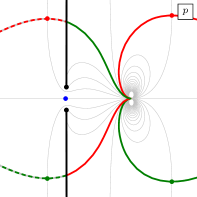
(a)

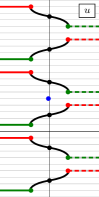
(b)

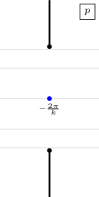
(c)

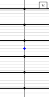
(d)

Figure 31: The $p$ and $u$ planes with $k=5$ in the relativistic limit. Figures LABEL:sub@fig:p-plane-h01-k5 and LABEL:sub@fig:u-plane-h01-k5 show the $p$ and $u$ planes for $h=1/10$. As we lower $h$ even more the scallion and kidney cuts in the $u$ plane move further away from the imaginary axis and the black cuts become flatter. The relativistic limit zooms in at a narrow strip around the imaginary axis in the $u$ plane, which corresponds to the a region close to $p=-2\pi/k$ in the $p$ plane, as shown in figures LABEL:sub@fig:p-plane-h0-k5 and LABEL:sub@fig:u-plane-h0-k5. The $p$ plane now looks like that of a standard massive relativistic excitation, and the $u$ plane goes to the corresponding rapidity plane. The blue dots in each plot show the location of an excitation with $p=-2\pi/k$.

In this sub-section we consider the relativistic limit of the mixed-flux odd dressing phases found above. Relativistic limits have been used in integrable $\text{AdS}_{3}$ models in R-R backgrounds [33] to investigate massless modes, where a difference form of the S matrix and dressing phases was observed [40, 41], leading to novel expressions for massless dressing factors. In mixed-flux backgrounds such limits helped identify a close relationship to relativistic integrable models [42, 43] as well as q-deformed holographic ones [44, 45, 46]. In [21] a modified version of such relativistic limit was proposed, in which the Hopf algebra and hence S matrix and dressing phases were the same as in [41], but a different scaling of momentum was introduced. In this limit, $h\rightarrow 0$ and momentum is expanded around

$$p_{\mbox{\tiny L}}=-\frac{2\pi m}{k},\qquad p_{\mbox{\tiny R}}=\frac{2\pi m}{k},$$ (6.22)

with the corrections scaling with $h$

$$p_{\mbox{\tiny L}} =-\frac{2\pi m}{k}+\frac{4\pi h}{k}\left|\sin\left(\frac{m\pi}{k}\right)\right|\sinh\vartheta,$$ (6.23)

$$p_{\mbox{\tiny R}} =+\frac{2\pi m}{k}+\frac{4\pi h}{k}\left|\sin\left(\frac{m\pi}{k}\right)\right|\sinh\vartheta.$$

Above, $\vartheta$ is a direct analogue of the rapidity variable present in relativistic integrable models. Notice that in taking this limit we are zooming in on momenta between the scallions and kidneys, in other words on

$$p_{\mbox{\tiny L}}\in(-2\pi,0),\qquad\qquad p_{\mbox{\tiny R}}\in(0,2\pi).$$ (6.24)

Furthermore, in the limit the $E_{\mbox{\tiny I}}$ branch-points inside those regions move closer to the real axis and the effective dynamics, to leading order, matches that of a massive relativistic theory. Similarly, the $u$ variable becomes

$$u(x)\rightarrow-\frac{k}{\pi h}\left(\vartheta-i\pi\right),$$ (6.25)

in other words, up to some simple shifts and rescalings we can identify $u$ and $\vartheta$. Indeed, as shown in figure 31, in this limit the $(-2\pi,0)$ sheet of the $u$-plane matches the usual $\theta$ plane of relativistic theories. From (2.16) we note that

$$s\rightarrow\infty,\qquad\qquad s^{-1}\rightarrow 0.$$ (6.26)

It is worth pointing out that the expansion around the momenta in (6.22), which restricts the momenta to lie on the sheets (6.24) de facto puts an upper bound on the bound state number to be no more than $k$. This is because bound states with $m>k$ and $p$ in the range (6.22) are related to states with bound state number $m-k$ but momentum $p+2\pi$, as we discuss in section 7.1.2. The latter states necessarily decouple in the relativistic limit, since their momenta are not near the minimal values (6.22).

In this relativistic limit the crossing equations [41] can be solved [41, 21], with an explicit expression in terms of Barnes G-function, or equivelently an infinite product of ratios of $\Gamma$ functions for both dressing phases given in [21]. While those expressions are complicated, the $\vartheta$ derivative of the dressing phases is simple

$$\partial_{\vartheta}\theta_{\mathrlap{\mbox{\tiny L}\mbox{\tiny L}}\phantom{\mbox{\tiny R}\mbox{\tiny R}},\,\mbox{\tiny FPS}} =\frac{\sin\frac{\pi}{k}}{\cosh\vartheta-\cos\frac{2\pi}{k}}\Bigl{(}\frac{2}{k}\cos\frac{\pi}{k}-\frac{\vartheta}{\pi}\coth\frac{\vartheta}{2}\sin\frac{\pi}{k}\Bigr{)}$$ (6.27)

$$\partial_{\vartheta}\theta_{\mathrlap{\mbox{\tiny R}\mbox{\tiny L}}\phantom{\mbox{\tiny R}\mbox{\tiny R}},\,\mbox{\tiny FPS}} =\frac{\sin\frac{\pi}{k}}{\cosh\vartheta+\cos\frac{2\pi}{k}}\Bigl{(}\bigl{(}1-\frac{2}{k}\bigr{)}\cos\frac{\pi}{k}+\frac{\vartheta}{\pi}\tanh\frac{\vartheta}{2}\sin\frac{\pi}{k}\Bigr{)}$$

where $\vartheta\equiv\vartheta_{1}-\vartheta_{2}$.

We would like to compare this with relativistic limit of the exact odd phases and scalar factors found in the previous sub-sections. The expressions for $\chi_{\mathrlap{\mbox{\tiny L}\mbox{\tiny L}}\phantom{\mbox{\tiny R}\mbox{\tiny R}}}$ and $\chi_{\mathrlap{\mbox{\tiny R}\mbox{\tiny L}}\phantom{\mbox{\tiny R}\mbox{\tiny R}}}$ given in section 6.1 are valid on the $(0,2\pi)$ Zhukovsky sheets with the logarithms appearing in these expressions being on the principal branch. To compare to the relativistic limit we need to analytically continue all left momenta to the $(-2\pi,0)$ sheet as discussed in section 2.3. When analytically continuing $x^{\pm}_{\mbox{\tiny L}}$ and $y^{\pm}_{\mbox{\tiny L}}$ to the $(-2\pi,0)$ region via path $-1$ in figure 13, $x^{+}$ and $y^{+}$ cross the $(-\infty,-1/s]$ interval from below. As a result, the logarithms with arguments involving $x^{+}$ and $y^{+}$ continue to a different branch, for example

$$\log\left(x^{+}+s^{-1}\right)\longrightarrow\log\left(x^{+}+s^{-1}\right)-2\pi i.$$ (6.28)

However, the complete expression for $\chi_{\mathrlap{\mbox{\tiny L}\mbox{\tiny L}}\phantom{\mbox{\tiny R}\mbox{\tiny R}}}$ is analytic across $(-\infty,-1/s]$ and, as one can check explicitly, the change in branches cancels between the integral and non-integral terms in (6.3). For analytic continuation of $\chi_{\mathrlap{\mbox{\tiny R}\mbox{\tiny L}}\phantom{\mbox{\tiny R}\mbox{\tiny R}}}$ in $y^{\pm}$ to the $(-2\pi,0)$ sheet, it is useful to use (6.8). While the integral part of the expression explicitly has no cuts along path $-1$, the non-integral terms on the other hand do not. However, it is straightforward to check that $e^{-2i\theta_{\mathrlap{\mbox{\tiny R}\mbox{\tiny L}}\phantom{\mbox{\tiny R}\mbox{\tiny R}}}}$ has no cuts. As a result, we can also use the principal branch of the logarithm in (6.3) when finding the relativistic limit of $\chi_{\mathrlap{\mbox{\tiny L}\mbox{\tiny L}}\phantom{\mbox{\tiny R}\mbox{\tiny R}}}$ and $\chi_{\mathrlap{\mbox{\tiny R}\mbox{\tiny L}}\phantom{\mbox{\tiny R}\mbox{\tiny R}}}$.

It is then straightforward to check that in the relativistic limit the non-integral part of $\chi_{\mathrlap{\mbox{\tiny L}\mbox{\tiny L}}\phantom{\mbox{\tiny R}\mbox{\tiny R}}}$ in (6.3) cancels out in $\theta_{\mathrlap{\mbox{\tiny L}\mbox{\tiny L}}\phantom{\mbox{\tiny R}\mbox{\tiny R}}}$. Similarly, the non-integral part in the first line of $\chi_{\mathrlap{\mbox{\tiny R}\mbox{\tiny L}}\phantom{\mbox{\tiny R}\mbox{\tiny R}}}$ in (6.3) cancels out in $\theta_{\mathrlap{\mbox{\tiny R}\mbox{\tiny L}}\phantom{\mbox{\tiny R}\mbox{\tiny R}}}$, while the non-integral term on the second line cancels the contribution of the rational term in $A_{\mathrlap{\mbox{\tiny R}\mbox{\tiny L}}\phantom{\mbox{\tiny R}\mbox{\tiny R}},\text{odd}}^{2}$ in (6.1).

Turning to the integral parts of $\chi_{\mathrlap{\mbox{\tiny L}\mbox{\tiny L}}\phantom{\mbox{\tiny R}\mbox{\tiny R}}}$ and $\chi_{\mathrlap{\mbox{\tiny R}\mbox{\tiny L}}\phantom{\mbox{\tiny R}\mbox{\tiny R}}}$, we note that in the relativistic limit

$$y^{\pm}\partial_{y^{\pm}}\rightarrow\partial_{\vartheta}.$$ (6.29)

Using this, we find

$$y^{\pm}\partial_{y^{\pm}}\chi_{\mathrlap{\mbox{\tiny L}\mbox{\tiny L}}\phantom{\mbox{\tiny R}\mbox{\tiny R}}}(x^{\pm^{\prime}},y^{\pm})\longrightarrow\frac{1}{2\pi}\frac{e^{\theta_{2}\mp\frac{i\pi}{k}}}{e^{\theta_{1}\mp^{\prime}\frac{i\pi}{k}}-e^{\theta_{2}\mp\frac{i\pi}{k}}}\left(\log\left(e^{\theta_{1}\mp^{\prime}\frac{i\pi}{k}}\right)-\log\left(e^{\theta_{2}\mp\frac{i\pi}{k}}\right)\right),$$ (6.30)

from which one can check that the relativistic limit of our $\partial_{\vartheta}\theta_{\mathrlap{\mbox{\tiny L}\mbox{\tiny L}}\phantom{\mbox{\tiny R}\mbox{\tiny R}}}$ reduces to the expression in (6.27). Similarly, the integral part of $\chi_{\mathrlap{\mbox{\tiny R}\mbox{\tiny L}}\phantom{\mbox{\tiny R}\mbox{\tiny R}}}$ gives in the relativistic limit

$$y^{\pm}\partial_{y^{\pm}}\chi_{\mathrlap{\mbox{\tiny R}\mbox{\tiny L}}\phantom{\mbox{\tiny R}\mbox{\tiny R}}}(x^{\pm^{\prime}},y^{\pm})\longrightarrow-\frac{1}{2\pi}\frac{e^{\theta_{2}\mp\frac{i\pi}{k}}}{e^{\theta_{1}\mp^{\prime}\frac{i\pi}{k}}+e^{\theta_{2}\mp\frac{i\pi}{k}}}\left(\log\left(e^{\theta_{1}\mp^{\prime}\frac{i\pi}{k}}\right)-\log\left(e^{\theta_{2}\mp\frac{i\pi}{k}}\right)\right),$$ (6.31)

from which one can check that the relativistic limit of our $\partial_{\vartheta}\theta_{\mathrlap{\mbox{\tiny R}\mbox{\tiny L}}\phantom{\mbox{\tiny R}\mbox{\tiny R}}}$ reduces to the expression in (6.27).

In addition to matching the dressing phase in the relativistic limit we can also consider the even matrix elements. If we assume that the even phase becomes trivial in the relativistic limit we find

$$A_{\mathrlap{\mbox{\tiny L}\mbox{\tiny L}}\phantom{\mbox{\tiny R}\mbox{\tiny R}},\text{even}}^{2} \approx\frac{\sinh\bigl{(}\frac{\pi h}{2k}\bigl{(}u_{\mbox{\tiny L}}(x^{-})-u_{\mbox{\tiny L}}(y^{+})\bigr{)}\bigr{)}}{\sinh\bigl{(}\frac{\pi h}{2k}\bigl{(}u_{\mbox{\tiny L}}(x^{+})-u_{\mbox{\tiny L}}(y^{-})\bigr{)}\bigr{)}}\sigma_{\mathrlap{\mbox{\tiny L}\mbox{\tiny L}}\phantom{\mbox{\tiny R}\mbox{\tiny R}},\text{even}}^{-2}(p,q)\to\frac{\sinh\bigl{(}\frac{\vartheta}{2}+\frac{i\pi}{k}\bigr{)}}{\sinh\bigl{(}\frac{\vartheta}{2}-\frac{i\pi}{k}\bigr{)}},$$ (6.32)

$$A_{\mathrlap{\mbox{\tiny R}\mbox{\tiny L}}\phantom{\mbox{\tiny R}\mbox{\tiny R}},\text{even}}^{2} \approx\frac{\sinh\bigl{(}\frac{\pi h}{2k}\bigl{(}u_{\mbox{\tiny R}}(x^{+})-u_{\mbox{\tiny L}}(y^{-})\bigr{)}\bigr{)}}{\sinh\bigl{(}\frac{\pi h}{2k}\bigl{(}u_{\mbox{\tiny R}}(x^{-})-u_{\mbox{\tiny L}}(y^{+})\bigr{)}\bigr{)}}\sigma_{\mathrlap{\mbox{\tiny R}\mbox{\tiny L}}\phantom{\mbox{\tiny R}\mbox{\tiny R}},\text{even}}^{-2}(p,q)\to\frac{\cosh\bigl{(}\frac{\vartheta}{2}-\frac{i\pi}{k}\bigr{)}}{\cosh\bigl{(}\frac{\vartheta}{2}+\frac{i\pi}{k}\bigr{)}}.$$

This perfectly agrees with the relativistic “CDD” factors of [21].

We have further checked that in a neighbourhood of physical values of momenta near (6.22) our odd phase matches numerically the one in [21]. Together with the matching of the crossing equations, even phase and the derivatives above this completes the check that our S matrix reduces in the relativistic limit to the one in [21]. In particular, it indicates that the even part of a putative mixed-flux BES phase will trivialise in the relativistic limit.

7 Constraints from the bound state S matrix

In integrable models the bound-state S matrix, i.e., the S matrix describing scattering of a bound state with either a fundamental excitation or a second bound state, can be obtained from the S matrix for two fundamental excitations through the fusion procedure. [47, 48, 49, 50] This procedure is a bit simpler in the $\text{AdS}_{3}\times\mathrm{S}^{3}\times\mathrm{T}^{4}$ world-sheet theory than in a general integral field theory, because all short representations $\mathrm{psu}(1|1)^{4}_{\text{ce}}$ are the same up to the values of the central charges, and it is straightforward to check that the matrix part of the S matrix fuses.

7.1 Special bound state configurations

The mixed-flux theory contains some special bound state configurations which do not have direct counterparts in the pure R-R model. They all have to do with configuration with bound state numbers close to $k$. As we will see in this section these configuration provide additional constraints on the world-sheet S matrix.

7.1.1 Singlet states

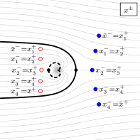
Figure 32: Two singlet configurations. The blue filled dots show a singlet made up of excitations outside the scallion, while the red hollow dots show a singlet made up of excitations sitting between the scallion and the kidney. Note that all such singlets carry exactly the same charges.

Consider a state consisting of a bound state with $m=k-1$ with momentum $p\in(0,2\pi)$, described by bound state Zhukovsky parameters $X^{\pm}=\Xi_{\mbox{\tiny L}}^{\pm}(p,k-1)$, plus a fundamental crossed excitation with momentum $-2\pi-p$. According to equation (2.19), the crossed excitation has parameters $\bar{x}^{\pm}=\Xi_{\mbox{\tiny L}}^{\mp}(p,k-1)$. The full state has total momentum $-2\pi$ and vanishing energy and charge. The $\mathrm{psu}(1|1)^{4}_{\text{ce}}$ representation coefficients only depend on $p$ up to factors of $2\pi$, so this state is a singlet of the $\mathrm{psu}(1|1)^{4}_{\text{ce}}$ algebra. Since the dynamics of the theory, i.e., the S matrix, is fully determined through $\mathrm{psu}(1|1)^{4}_{\text{ce}}$ representation theory we expect this singlet state to completely decouple from the theory, which means that is should scatter trivially with any other state.

This construction of a singlet as a $k-1$ physical bound state with momentum $p$ plus a crossed fundamental excitation with momentum $-2\pi-p$ works for $p$ in any range. Moreover, we can generalise it by starting with a bound state with $nk-1$ excitations and a crossed excitation with momentum $-2\pi(n+1)-p$, which leads to a singlet with total momentum $-2\pi(n+1)$. Figure 32 shows two such singlet configurations.

We can also decompose the singlet in various ways. The exact same state can be viewed as a physical L bound state with bound state number $m$ with $1\leq m<k-1$ and a crossed L bound state with bound state number $k-m$.

7.1.2 The $m=k+1$ bound state as a fundamental excitation

Let us now consider an $m=k+1$ bound state. It is described by the parameters

$$x_{1}^{+} =\Xi_{\mbox{\tiny L}}^{+}(p,k+1),$$ (7.1)

$$x_{1}^{-}=x_{2}^{+} =\Xi_{\mbox{\tiny L}}^{+}(q_{1},k-1),$$

$$\mathmakebox[\widthof{{}={}}][c]{\vdots}$$

$$x_{k}^{-}=x_{k+1}^{+} =\Xi_{\mbox{\tiny L}}^{-}(q_{1},k-1),$$

$$x_{k+1}^{-} =\Xi_{\mbox{\tiny L}}^{-}(p,k+1).$$

We now rename the parameters

$$\begin{gathered}x^{+}=x_{1}^{+},\quad x^{-}=x_{k+1}^{-},\quad\bar{y}^{+}=x_{k+1}^{+},\quad\bar{y}^{-}=x_{1}^{-},\\ y_{j}^{\pm}=x_{j+1}^{\pm},\quad\text{for $j=1,\dotsc,k-1$}.\end{gathered}$$ (7.2)

The parameters $y_{j}^{\pm}$ and $\bar{y}^{\pm}$ describe a singlet of exactly the same form discussed above. It contributes $-2\pi$ to the momentum but has no energy or charge. We are left with $x^{\pm}=\Xi_{\mbox{\tiny L}}^{\pm}(p,k+1)$. This is exactly the parameters for a fundamental physical excitation with momentum $p+2\pi$.

This construction too works for any momentum range. Since we expect the singlet state to decouple from the theory we are left to conclude that a $m=k+1$ bound state with momentum $p$ should scatter in the same way as a fundamental excitation with momentum $p+2\pi$. We may also repeat the construction $n$ times and we are led to conclude that an $m=nk+1$ bound state with momentum $p$ should be identified with a fundamental excitation at momentum $p+2\pi n$. If we did not make such identification, we would have an infinite degeneracy of representations which would lead to an unphysically large spectrum.

Note that this identification means that we get an upper bound on the bound state number $m\leq k$ while the momentum $p$ can take any real value.

7.1.3 The $m=k-1$ bound state as an R excitation

Let us now consider an $m=k-1$ bound state. As we saw above, we can construct a singlet from this bound state by adding a fundamental crossed excitation. Hence, the $m=k-1$ bound state acts as an anti-particle to the fundamental excitation. But from representation theory we expect the anti-particle of an L excitation to be an R excitation. Indeed if we let the bound state have momentum $p-2\pi$ we find that it has energy

$$E_{\mbox{\tiny L}}(p-2\pi,m=k-1)=\sqrt{(1-\mathchar 22\relax\mkern-9.0mukp)^{2}+4h^{2}\sin^{2}\frac{p}{2}}=E_{\mbox{\tiny R}}(p,m=1)$$ (7.3)

which is exactly the same as that of an R excitation of momentum $p$. Similarly, these two states carry the same charge. As mentioned above, $\mathrm{psu}(1|1)^{4}_{\text{ce}}$ representation theory only cares about the momentum up to shifts of $2\pi$. This means that from the perspective of representations, and thus the S matrix, the $m=k-1$ bound state at momentum $p-2\pi$ is indistinguishable from a fundamental R excitation with momentum $p$.

To make this identification more precise, we note that the Zhukovsky parameters $X^{\pm}$ for an $m=k-1$ bound state with momentum $p-2\pi$ and the parameters $x_{\mbox{\tiny R}}^{\pm}$ for a fundamental R excitation of momentum $p$ satisfy

$$X^{\pm}(p-2\pi,k-1)=-\frac{1-\mathchar 22\relax\mkern-9.0mukp-\sqrt{(1-\mathchar 22\relax\mkern-9.0mukp)^{2}+4h^{2}\sin^{2}\frac{p}{2}}}{2h\sin\frac{p}{2}}e^{\pm\frac{ip}{2}}=\frac{1}{x_{\mbox{\tiny R}}^{\mp}(p)}$$ (7.4)

It is straightforward to check for the matrix part of the S matrix [7] that this replacement maps the LL S matrix to the S matrices for RL, LR and RR scattering. However, the identification does put constraints on the scalar factors of these S matrices.

7.1.4 The $m=k$ bound state as a massless excitation

Finally we will consider a physical bound state with $m=k$. Such a state has energy

$$E_{\mbox{\tiny L}}(p,m=k)=\sqrt{\mathchar 22\relax\mkern-9.0muk^{2}(p+2\pi)^{2}+4h^{2}\sin^{2}\frac{p}{2}}=E_{\mbox{\tiny L}}(p+2\pi,m=0).$$ (7.5)

When such a bound state exists it will thus look just like a massless excitation in a higher momentum region. Taking into account the identification of an $m=k-1$ L bound state with momentum $p$ and an R fundamental excitation of momentum $p+2\pi$, this massless mode can also be seen as a bound state between fundamental L and R excitations.

In summary, we have shown that the full massive sector of the mixed-flux world-sheet theory is captured by considering only L excitations with bound state numbers in the range $m\leq k$ and any momenta.

7.2 Constraints on the S matrix

In this section we will check some of the above constraints on the S matrix, focusing on the LL S matrix in the $(-2\pi,0)$ region. As discussed in section 6 the even part of the highest weight matrix element takes the form

$$A_{\mathrlap{\mbox{\tiny L}\mbox{\tiny L}}\phantom{\mbox{\tiny R}\mbox{\tiny R}},\text{even}}^{2}(x^{\pm},y^{\pm})=\frac{S\bigl{[}u_{\mbox{\tiny L}}(x^{-})-u_{\mbox{\tiny L}}(y^{+})\bigr{]}}{S\bigl{[}u_{\mbox{\tiny L}}(x^{+})-u_{\mbox{\tiny L}}(y^{-})\bigr{]}}\sigma_{\mathrlap{\mbox{\tiny L}\mbox{\tiny L}}\phantom{\mbox{\tiny R}\mbox{\tiny R}},\text{even}}^{-2}(x^{\pm},y^{\pm})$$ (7.6)

where we have introduced the functions

$$S[u]=\sinh\bigl{(}\tfrac{\pi h}{2k}u\bigr{)},\qquad C[u]=\cosh\bigl{(}\tfrac{\pi h}{2k}u\bigr{)},$$ (7.7)

satisfying

$$S\bigl{[}u\pm\tfrac{ik}{h}\bigr{]}=\pm iC[u],\qquad S\bigl{[}u\pm\tfrac{2ik}{h}\bigr{]}=-S[u],\qquad C\bigl{[}u\pm\tfrac{2ik}{h}\bigr{]}=-C[u].$$ (7.8)

It is straightforward to fuse this matrix element $m$ times

$$A_{\mbox{\tiny L}^{m}\mbox{\tiny L},\text{even}}^{2}(X^{\pm},y^{\pm}) =\frac{S\bigl{[}u_{\mbox{\tiny L}}(X^{-})-u_{\mbox{\tiny L}}(y^{+})\bigr{]}}{S\bigl{[}u_{\mbox{\tiny L}}(X^{+})-u_{\mbox{\tiny L}}(y^{-})\bigr{]}}\frac{S\bigl{[}u_{\mbox{\tiny L}}(X^{-})-u_{\mbox{\tiny L}}(y^{-})\bigr{]}}{S\bigl{[}u_{\mbox{\tiny L}}(X^{+})-u_{\mbox{\tiny L}}(y^{+})\bigr{]}}\sigma_{\mbox{\tiny L}^{m}\mbox{\tiny L},\text{even}}^{-2}(X^{\pm},y^{\pm}).$$ (7.9)

$$=\frac{S\bigl{[}U_{\mbox{\tiny L}}-v_{\mbox{\tiny L}}-\frac{i(m+1)}{h}\bigr{]}}{S\bigl{[}U_{\mbox{\tiny L}}-v_{\mbox{\tiny L}}+\frac{i(m+1)}{h}\bigr{]}}\frac{S\bigl{[}U_{\mbox{\tiny L}}-v_{\mbox{\tiny L}}-\frac{i(m-1)}{h}\bigr{]}}{S\bigl{[}U_{\mbox{\tiny L}}-v_{\mbox{\tiny L}}+\frac{i(m-1)}{h}\bigr{]}}\sigma_{\mbox{\tiny L}^{m}\mbox{\tiny L},\text{even}}^{-2}(X^{\pm},y^{\pm}),$$

where we have introduced $U_{\mbox{\tiny L}}$ and $v_{\mbox{\tiny L}}$ defined through the relations

$$u_{\mbox{\tiny L}}(X^{\pm})=U_{\mbox{\tiny L}}\pm\frac{im}{h},\qquad u_{\mbox{\tiny L}}(y^{\pm})=v_{\mbox{\tiny L}}\pm\frac{i}{h}.$$ (7.10)

In particular for $m=k-1$ we get

$$A_{\mbox{\tiny L}^{(k-1)}\mbox{\tiny L},\text{even}}^{2}(X^{\pm},y^{\pm}) =\frac{S\bigl{[}U_{\mbox{\tiny L}}-v_{\mbox{\tiny L}}-\frac{ik}{h}\bigr{]}}{S\bigl{[}U_{\mbox{\tiny L}}-v_{\mbox{\tiny L}}+\frac{ik}{h}\bigr{]}}\frac{S\bigl{[}U_{\mbox{\tiny L}}-v_{\mbox{\tiny L}}+\frac{2i}{h}-\frac{ik}{h}\bigr{]}}{S\bigl{[}U_{\mbox{\tiny L}}-v_{\mbox{\tiny L}}-\frac{2i}{h}+\frac{ik}{h}\bigr{]}}\sigma_{\mbox{\tiny L}^{(k-1)}\mbox{\tiny L},\text{even}}^{-2}(X^{\pm},y^{\pm})$$

$$=\frac{C\bigl{[}U_{\mbox{\tiny L}}-v_{\mbox{\tiny L}}+\frac{2i}{h}\bigr{]}}{C\bigl{[}U_{\mbox{\tiny L}}-v_{\mbox{\tiny L}}-\frac{2i}{h}\bigr{]}}\sigma_{\mbox{\tiny L}^{(k-1)}\mbox{\tiny L},\text{even}}^{-2}(X^{\pm},y^{\pm})$$ (7.11)

To compare this with the RL matrix element $A_{\mathrlap{\mbox{\tiny R}\mbox{\tiny L}}\phantom{\mbox{\tiny R}\mbox{\tiny R}}}^{2}$ we should use the relations $X^{\pm}=1/x_{\mbox{\tiny R}}^{\mp}$. In terms of the $u$-plane this translates to

$$u_{\mbox{\tiny L}}(X^{+})=u_{\mbox{\tiny R}}(x_{\mbox{\tiny R}}^{-})+\frac{2ik}{h},\qquad u_{\mbox{\tiny L}}(X^{-})=u_{\mbox{\tiny R}}(x_{\mbox{\tiny R}}^{+}),$$ (7.12)

or

$$u_{\mbox{\tiny R}}=U_{\mbox{\tiny L}}-\frac{ik}{h}.$$ (7.13)

Inserting this into the above matrix element we find

$$A_{\mbox{\tiny L}^{(k-1)}\mbox{\tiny L},\text{even}}^{2}(1/x_{\mbox{\tiny R}}^{\mp},y^{\pm}) =\frac{S\bigl{[}u_{\mbox{\tiny R}}(x_{\mbox{\tiny R}}^{+})-u_{\mbox{\tiny L}}(y^{-})\bigr{]}}{S\bigl{[}u_{\mbox{\tiny R}}(x_{\mbox{\tiny R}}^{-})-u_{\mbox{\tiny L}}(y^{+})\bigr{]}}\sigma_{\mbox{\tiny L}^{(k-1)}\mbox{\tiny L},\text{even}}^{-2}(1/x_{\mbox{\tiny R}}^{\mp},y^{\pm})$$ (7.14)

$$=\frac{S\bigl{[}u_{\mbox{\tiny R}}-v_{\mbox{\tiny L}}+\frac{2i}{h}\bigr{]}}{S\bigl{[}u_{\mbox{\tiny R}}-v_{\mbox{\tiny L}}-\frac{2i}{h}\bigr{]}}\sigma_{\mbox{\tiny L}^{(k-1)}\mbox{\tiny L},\text{even}}^{-2}(1/x_{\mbox{\tiny R}}^{\mp},y^{\pm}).$$

This exactly matches the even RL matrix element (6.19) as long as the even dressing phases satisfy the fusion condition by themselves

$$\sigma_{\mbox{\tiny L}^{(k-1)}\mbox{\tiny L},\text{even}}^{2}(1/x_{\mbox{\tiny R}}^{\mp},y^{\pm})=\sigma_{\mathrlap{\mbox{\tiny R}\mbox{\tiny L}}\phantom{\mbox{\tiny R}\mbox{\tiny R}},\text{even}}^{2}(x_{\mbox{\tiny R}}^{\pm},y^{\pm}).$$ (7.15)

Let us now turn to the odd S matrix element. Fusing the odd LL matrix element $k-1$ times we get

$$A_{\mbox{\tiny L}^{(k-1)}\mbox{\tiny L},\text{odd}}^{2}(1/x^{\mp},y^{\pm})=\Bigl{(}\frac{\alpha(1/x^{+})}{\alpha(1/x^{-})}\Bigr{)}^{\!\!1/k}\Bigl{(}\frac{\alpha(y^{+})}{\alpha(y^{-})}\Bigr{)}^{\!1-\frac{1}{k}}e^{-2i\theta_{\mathrlap{\mbox{\tiny L}\mbox{\tiny L}}\phantom{\mbox{\tiny R}\mbox{\tiny R}}}(1/x^{\mp},y^{\pm})}.$$ (7.16)

To compare this with the RL matrix element we first note that the RL phase in (6.3) can be rewritten (up to terms that do not contribute to $\theta_{\mathrlap{\mbox{\tiny R}\mbox{\tiny L}}\phantom{\mbox{\tiny R}\mbox{\tiny R}}}$) as

$$\chi_{\mathrlap{\mbox{\tiny R}\mbox{\tiny L}}\phantom{\mbox{\tiny R}\mbox{\tiny R}}}(x,y) =-\!\!\int_{s}^{-s^{-1}}\frac{dz}{2\pi}\frac{\log(y-z)}{\frac{1}{x}-z}-\frac{1}{4\pi}\log\frac{\frac{1}{x}+s}{\frac{1}{x}-s^{-1}}\bigl{(}\log(y+s^{-1})+\log(y-s)\bigr{)}$$ (7.17)

$$\qquad-\frac{i}{2}\operatorname{sign}(\mathop{\mathrm{Im}}x)\Bigl{(}\log\bigl{(}y-\frac{1}{x}\bigr{)}-\frac{1}{2}\bigl{(}\log(y+s^{-1})+\log(y-s)\bigr{)}\Bigr{)},$$

where the first line equals $-\chi_{\mathrlap{\mbox{\tiny L}\mbox{\tiny L}}\phantom{\mbox{\tiny R}\mbox{\tiny R}}}(1/x,y)$. For a physical real momentum excitation $\mathop{\mathrm{Im}}x^{+}>0$ and $\mathop{\mathrm{Im}}x^{-}<0$ and we can use the expression in the second line above to simplify the rational terms in (6.1) to

$$A_{\mathrlap{\mbox{\tiny R}\mbox{\tiny L}}\phantom{\mbox{\tiny R}\mbox{\tiny R}},\text{odd}}^{2}(x^{\pm},y^{\pm})=\Bigl{(}\frac{\alpha(1/x^{+})}{\alpha(1/x^{-})}\Bigr{)}^{\!\!1/k}\Bigl{(}\frac{\alpha(y^{+})}{\alpha(y^{-})}\Bigr{)}^{\!1-\frac{1}{k}}e^{2i\theta_{\mathrlap{\mbox{\tiny L}\mbox{\tiny L}}\phantom{\mbox{\tiny R}\mbox{\tiny R}}}(1/x^{\pm},y^{\pm})},$$ (7.18)

which perfectly matches what we got by fusing the odd LL matrix element. Even though we found this expression by assuming that the momentum of the $x^{\pm}$ excitation is real it is straight forward to extend it to the whole complex plane by picking up the right branch of the dressing phase.

Note that the $k-1$ times fused S matrix element (7.11) does not have an S channel pole. This means that we cannot extend it to an $m=k$ bound state. This has a direct parallel in the XXZ model [37]. However, in [39] it was pointed out that the XXZ model in fact does contain zero modes that correspond to $m=k$ bound states, even though they do not appear as solutions to the Bethe ansatz equations. Since our proposed scalar factor has the same form as the XXZ chain, we expect similar results to hold for $\text{AdS}_{3}$ also. In particular, this should clarify how massless states appear as a results of fusion. We hope to return to these questions in the near future.

Here we have focused our discussion about the relation between different bound states to the case where the bound state sits in the region between the scallion and the kidney. We expect similar results to hold in other momentum regions. For the odd part of the matrix elements the above calculation should be easy to translate to a different region. However, it is clear that the even part of the matrix element requires more care. Consider for example a $k+1$ bound state with momentum in $(0,2\pi)$ scattering with a fundamental excitation in the same region. From (6.11) we find

$$A_{\mbox{\tiny L}^{(k+1)}\mbox{\tiny L},\text{even}}^{2}(X^{\pm},y^{\pm})=\frac{u_{\mbox{\tiny L}}(X^{-})-u_{\mbox{\tiny L}}(y^{+})}{u_{\mbox{\tiny L}}(X^{+})-u_{\mbox{\tiny L}}(y^{-})}\frac{u_{\mbox{\tiny L}}(X^{+})-u_{\mbox{\tiny L}}(y^{+})}{u_{\mbox{\tiny L}}(X^{-})-u_{\mbox{\tiny L}}(y^{-})}\\ \times\frac{X^{+}}{X^{-}}\Bigl{(}\frac{y^{-}}{y^{+}}\Bigr{)}^{k+1}\sigma_{\mbox{\tiny L}^{(k+1)}\mbox{\tiny L},\text{even}}^{-2}(X^{\pm},y^{\pm}).$$ (7.19)

Since the rapidity plane is not periodic we cannot drop the second factor here. This matrix element should equal $A_{\mathrlap{\mbox{\tiny L}\mbox{\tiny L}}\phantom{\mbox{\tiny R}\mbox{\tiny R}},\text{even}}^{2}(p+2\pi,q)$ with two fundamental excitations. For this to be possible we need to pick up a compensating factor from the even dressing phase when we analytically continue from $p$ to $p+2\pi$. This should provide a test of the even dressing phase.

8 Conclusions

We have analysed the kinematical structure of worldsheet excitations in mixed-flux $\text{AdS}_{3}\times\mathrm{S}^{3}\times\mathrm{T}^{4}$ geometries and found a structure far richer than in the case of R-R backgrounds. Momenta of these excitations are no longer periodic and the related Zhukovsky variables have infinitely many sheets, which we have shown can be reached through analytic continuations around the singular $p=2\pi n$ ($n\in\mathbb{Z}$) points. Similarly, the variable $u$ that is commonly used in integrable holography has a mixed-flux generalisation for each pair of Zhukovsky sheets. We have identified one set of Zhukovsky sheets and corresponding $u$ variable, which exhibit a novel type of periodicity. Alongside this paper we include a graphics programme that can be used to visualise this complicted analytic structure for both fundamental and bound state excitations [14].

Using these analyticity insights, we have shown that excitations which appear fundamental are equivalent to bound states upon suitable shifts of momenta. Similarly, R excitations can be constructed from L bound states. These constraints place restrictions on the S matrix of the theory, particularly on its scalar factors. We have solved the odd part of the crossing equations and proposed scalar factors for the S matrices that have the correct pole structure for the bound state spectrum of the theory. Focusing on the $(-2\pi,0)$ momentum region, we showed that these odd dressing phases and scalar factors have the required properties under fusion. Further, we proposed a scalar factor closely resembling the XXZ model at a root of unity, i.e., with anisotropy of the form $\Delta=\cos\frac{\pi}{k}$. This factor ensures consistency with $u$-periodicity in this region, the correct bound-state simple poles expected in the theory, as well as the required properties under fusion.

Unlike $\text{AdS}_{5}$, integrable $\text{AdS}_{3}$ theories’ dressing factors remain non-trivial in the $h\rightarrow 0$ limit, both in R-R and mixed-flux cases, signalling the non-square-root nature of the branch points [27]. This is an important difference in the weakly-coupled regime: the $\text{AdS}_{5}$ case reduces to an XXX spin-chain in the $\mathrm{su}(2)$ sector, while in the $\text{AdS}_{3}$ case, depending on the momentum region we would get XXX or XXZ spin-chains, dressed by non-trivial phases. Intriguingly, this suggests that the planar spectrum of the WZW model deformed by the axion modulus should be governed by such “dressed” spin-chains.

Having gained a better understanding of the analyticity properties of the mixed-flux theory across the full range of $p$, we revisited its relativistic limit. Related limits were introduced in R-R backgrounds [33] where they led to a difference-form for the massless S matrix and dressing factors [40, 41], fixing certain potential CDD ambiguities and leading to novel expressions for massless dressing factors. Relativistic limits were also studied in mixed-flux backgrounds [41], where a close relationship to relativistic integrable models [42, 43] as well as q-deformed holographic ones [44, 45, 46] was identified. An improved version of this relativistic limit was proposed in [21], for which the Hopf algebra and hence S matrix and dressing phases were the same as in [41], but whose dispersion relation matched the bound-state structure more closely to the $\text{AdS}_{3}$ case. We showed that the correct way to interpret the relativistic limit is as coming from the region between the scallion and kidney, zooming in on momenta near the $E_{I}$ branch points, as illustrated in figure 31. As we explained, from this perspective the truncation of the bound state spectrum is natural, with all but a finite number of bound states decoupling because they can equivalently be viewed as states whose momenta are not near the minimal values (6.24). With these clarifications, we then showed that the odd dressing phase and scalar factors we have found in this paper reduce to the corresponding expressions given in [21, 41].

The relations between massless modes and bound states with shifted momenta discussed in section 7.1 suggests that wrapping corrections coming from massless and mixed mass effects may be easier to analyse in the mixed-flux setting than in the R-R case, because one may be able to view all modes as being massive, under suitable momentum shift. In light of this, it may be worth revisiting the findings of [51], as well as generalising the QSC computations of [52].

To complete the determination of the S matrix of mixed-flux backgorunds it remains to find the even dressing factors, which should amount to finding the mixed-flux generalisation of the BES phase. We leave this for future work. It would be interesting to understand the mixed-flux TBA and QSC and use them to solve the spectral problem on $\text{AdS}_{3}\times\mathrm{S}^{3}\times\mathrm{T}^{4}$ backgrounds. This would provide much needed data for testing the $\text{AdS}_{3}/\text{CFT}_{2}$ duality and understanding the connection to the $\operatorname{Sym}^{N}(\mathrm{T}^{4})$ dual CFT, the $k=1$ results using the hybrid formalism [53], as well as the appearance of integrability on the Higgs branch of the infrared limit of the D1-D5-brane gauge theory [54].

References

- Babichenko et al. [2010] A. Babichenko, B. Stefański, jr. and K. Zarembo, Integrability and the AdS3/CFT2 correspondence, JHEP 1003, 058 (2010), arxiv:0912.1723.
- Ohlsson Sax and Stefański [2011] O. Ohlsson Sax and B. Stefański, jr., Integrability, spin-chains and the AdS3/CFT2 correspondence, JHEP 1108, 029 (2011), arxiv:1106.2558.
- Cagnazzo and Zarembo [2012] A. Cagnazzo and K. Zarembo, B-field in AdS3/CFT2 correspondence and integrability, JHEP 1211, 133 (2012), arxiv:1209.4049.
- David and Sahoo [2008] J. R. David and B. Sahoo, Giant magnons in the D1-D5 system, JHEP 0807, 033 (2008), arxiv:0804.3267.
- David and Sahoo [2010] J. R. David and B. Sahoo, S-matrix for magnons in the D1-D5 system, JHEP 1010, 112 (2010), arxiv:1005.0501.
- Ohlsson Sax and Stefański [2018] O. Ohlsson Sax and B. Stefański, jr., Closed strings and moduli in AdS3/CFT2, JHEP 1805, 101 (2018), arxiv:1804.02023.
- Lloyd et al. [2015] T. Lloyd, O. Ohlsson Sax, A. Sfondrini and B. Stefański, jr., The complete worldsheet S matrix of superstrings on with mixed three-form flux, Nucl. Phys. B891, 570 (2015), arxiv:1410.0866.
- Borsato et al. [2013] R. Borsato, O. Ohlsson Sax, A. Sfondrini, B. Stefański, jr. and A. Torrielli, The all-loop integrable spin-chain for strings on : the massive sector, JHEP 1308, 043 (2013), arxiv:1303.5995.
- Borsato et al. [2014] R. Borsato, O. Ohlsson Sax, A. Sfondrini and B. Stefański, jr., Towards the all-loop worldsheet S matrix for , Phys. Rev. Lett. 113, 131601 (2014), arxiv:1403.4543.
- Borsato et al. [2014] R. Borsato, O. Ohlsson Sax, A. Sfondrini and B. Stefański, jr, The complete worldsheet S-matrix, JHEP 1410, 66 (2014), arxiv:1406.0453.
- Hoare et al. [2014] B. Hoare, A. Stepanchuk and A. Tseytlin, Giant magnon solution and dispersion relation in string theory in with mixed flux, Nucl. Phys. B879, 318 (2014), arxiv:1311.1794.
- Larsen and Martinec [1999] F. Larsen and E. J. Martinec, charges and moduli in the D1-D5 system, JHEP 9906, 019 (1999), hep-th/9905064.
- Maldacena and Ooguri [2001] J. M. Maldacena and H. Ooguri, Strings in and WZW model. I, J. Math. Phys. 42, 2929 (2001), hep-th/0001053.
- Ohlsson Sax [2023] O. Ohlsson Sax, PXU, 2023. Available at https://olofos.github.io/pxu-gui/.
- Gromov et al. [2015] N. Gromov, V. Kazakov, S. Leurent and D. Volin, Quantum spectral curve for arbitrary state/operator in AdS5/CFT4, JHEP 1509, 187 (2015), arxiv:1405.4857.
- Bombardelli et al. [2017] D. Bombardelli, A. Cavaglià, D. Fioravanti, N. Gromov and R. Tateo, The full quantum spectral curve for AdS4/CFT3, arxiv:1701.00473.
- Cavaglià et al. [2021] A. Cavaglià, N. Gromov, B. Stefański, jr. and A. Torrielli, Quantum spectral curve for AdS3/CFT2: a proposal, JHEP 2112, 048 (2021), arxiv:2109.05500.
- Ekhammar and Volin [2022] S. Ekhammar and D. Volin, Monodromy bootstrap for quantum spectral curves: from hubbard model to , JHEP 2203, 192 (2022), arxiv:2109.06164.
- Frolov and Sfondrini [2022] S. Frolov and A. Sfondrini, New dressing factors for , JHEP 2204, 162 (2022), arxiv:2112.08896.
- Beisert et al. [2006] N. Beisert, R. Hernández and E. López, A crossing-symmetric phase for , JHEP 0611, 070 (2006), hep-th/0609044.
- Frolov et al. [2023] S. Frolov, D. Polvara and A. Sfondrini, On mixed-flux worldsheet scattering in , JHEP 2311, 055 (2023), arxiv:2306.17553.
- Beisert et al. [2007] N. Beisert, B. Eden and M. Staudacher, Transcendentality and crossing, J. Stat. Mech. 0701, P01021 (2007), hep-th/0610251.
- Beisert et al. [2012] N. Beisert et al., Review of AdS/CFT integrability: An overview, Lett. Math. Phys. 99, 3 (2012), arxiv:1012.3982.
- Arutyunov and Frolov [2009] G. Arutyunov and S. Frolov, Foundations of the superstring. Part I, J. Phys. A A42, 254003 (2009), arxiv:0901.4937.
- Babichenko et al. [2014] A. Babichenko, A. Dekel and O. Ohlsson Sax, Finite-gap equations for strings on with mixed 3-form flux, JHEP 1411, 122 (2014), arxiv:1405.6087.
- Borsato et al. [2013] R. Borsato, O. Ohlsson Sax and A. Sfondrini, A dynamic S-matrix for AdS3/CFT2, JHEP 1304, 113 (2013), arxiv:1211.5119.
- Borsato et al. [2013] R. Borsato, O. Ohlsson Sax, A. Sfondrini, B. Stefański, jr. and A. Torrielli, Dressing phases of AdS3/CFT2, Phys. Rev. D88, 066004 (2013), arxiv:1306.2512.
- Ohlsson Sax and Stefański [2020] O. Ohlsson Sax and B. Stefański, jr., On the singularities of the R-R S matrix, J. Phys. A 53, 155402 (2020), arxiv:1912.04320.
- Borsato et al. [2016] R. Borsato, O. Ohlsson Sax, A. Sfondrini and B. Stefański, jr., On the spectrum of strings with Ramond-Ramond flux, J. Phys. A49, 41LT03 (2016), arxiv:1605.00518.
- Borsato et al. [2017] R. Borsato, O. Ohlsson Sax, A. Sfondrini, B. Stefański, jr. and A. Torrielli, On the dressing factors, Bethe equations and Yangian symmetry of strings on , J. Phys. A50, 024004 (2017), arxiv:1607.00914.
- [31] A. Cavaglià and S. Ekhammar. Unpublished. See presentation at IGST 2022.
- [32] A. Cavaglià, S. Ekhammar, S. Majumder, B. Stefański, jr. and A. Torrielli. Unpublished.
- Bombardelli et al. [2018] D. Bombardelli, B. Stefański and A. Torrielli, The low-energy limit of AdS3/CFT2 and its TBA, JHEP 1810, 177 (2018), arxiv:1807.07775.
- Castillejo et al. [1956] L. Castillejo, R. H. Dalitz and F. J. Dyson, Low’s scattering equation for the charged and neutral scalar theories, Phys. Rev. 101, 453 (1956).
- Dorey et al. [2007] N. Dorey, D. M. Hofman and J. M. Maldacena, On the singularities of the magnon S-matrix, Phys. Rev. D76, 025011 (2007), hep-th/0703104.
- Beisert et al. [2004] N. Beisert, V. Dippel and M. Staudacher, A novel long range spin chain and planar super Yang- Mills, JHEP 0407, 075 (2004), hep-th/0405001.
- Fabricius and McCoy [2001] K. Fabricius and B. M. McCoy, Bethe’s equation is incomplete for the XXZ model at roots of unity, J. Statist. Phys. 103, 647 (2001), cond-mat/0009279.
- Baxter [2002] R. J. Baxter, Completeness of the Bethe ansatz for the six and eight vertex models, J. Statist. Phys. 108, 1 (2002), cond-mat/0111188.
- Braak and Andrei [2001] D. Braak and N. Andrei, On the spectrum of the XXZ-chain at roots of unity, Journal of statistical physics 105, 677 (2001), cond-mat/0106593.
- Fontanella and Torrielli [2019] A. Fontanella and A. Torrielli, Geometry of massless scattering in integrable superstring, JHEP 1906, 116 (2019), arxiv:1903.10759.
- Fontanella et al. [2019] A. Fontanella, O. Ohlsson Sax, B. Stefański, jr. and A. Torrielli, The effectiveness of relativistic invariance in , JHEP 1907, 105 (2019), arxiv:1905.00757.
- Fendley and Intriligator [1992] P. Fendley and K. A. Intriligator, Scattering and thermodynamics of fractionally charged supersymmetric solitons, Nucl. Phys. B 372, 533 (1992), hep-th/9111014.
- Fendley and Intriligator [1992] P. Fendley and K. A. Intriligator, Scattering and thermodynamics in integrable theories, Nucl. Phys. B 380, 265 (1992), hep-th/9202011.
- Arutyunov et al. [2012] G. Arutyunov, M. de Leeuw and S. J. van Tongeren, The quantum deformed mirror TBA I, JHEP 1210, 090 (2012), arxiv:1208.3478.
- Arutyunov et al. [2013] G. Arutyunov, M. de Leeuw and S. J. van Tongeren, The quantum deformed mirror TBA II, JHEP 1302, 012 (2013), arxiv:1210.8185.
- Hoare et al. [2013] B. Hoare, T. J. Hollowood and J. L. Miramontes, Restoring unitarity in the q-deformed world-sheet S-matrix, JHEP 1310, 050 (2013), arxiv:1303.1447.
- Roiban [2007] R. Roiban, Magnon bound-state scattering in gauge and string theory, JHEP 0704, 048 (2007), hep-th/0608049.
- Dorey [2006] N. Dorey, Magnon bound states and the AdS/CFT correspondence, J. Phys. A39, 13119 (2006), hep-th/0604175.
- Arutyunov and Frolov [2007] G. Arutyunov and S. Frolov, On string S-matrix, bound states and TBA, JHEP 0712, 024 (2007), arxiv:0710.1568.
- Arutyunov and Frolov [2008] G. Arutyunov and S. Frolov, The S-matrix of string bound states, Nucl. Phys. B804, 90 (2008), arxiv:0803.4323.
- Abbott and Aniceto [2016] M. C. Abbott and I. Aniceto, Massless Lüscher terms and the limitations of the asymptotic Bethe ansatz, Phys. Rev. D93, 106006 (2016), arxiv:1512.08761.
- Cavaglià et al. [2022] A. Cavaglià, S. Ekhammar, N. Gromov and P. Ryan, Exploring the quantum spectral curve for AdS3/CFT2, arxiv:2211.07810.
- Eberhardt et al. [2018] L. Eberhardt, M. R. Gaberdiel and R. Gopakumar, The worldsheet dual of the symmetric product CFT, arxiv:1812.01007.
- Ohlsson Sax et al. [2015] O. Ohlsson Sax, A. Sfondrini and B. Stefański, jr., Integrability and the conformal field theory of the Higgs branch, JHEP 1506, 103 (2015), arxiv:1411.3676.