Contact-Implicit MPC:
Controlling Diverse Quadruped Motions
Without Pre-Planned Contact Modes or Trajectories

Abstract

This paper presents a contact-implicit model predictive control (MPC) framework for the real-time discovery of multi-contact motions, without predefined contact mode sequences or foothold positions. This approach utilizes the contact-implicit differential dynamic programming (DDP) framework, merging the hard contact model with a linear complementarity constraint. We propose the analytical gradient of the contact impulse based on relaxed complementarity constraints to further the exploration of a variety of contact modes. By leveraging a hard contact model-based simulation and computation of search direction through a smooth gradient, our methodology identifies dynamically feasible state trajectories, control inputs, and contact forces while simultaneously unveiling new contact mode sequences. However, the broadened scope of contact modes does not always ensure real-world applicability. Recognizing this, we implemented differentiable cost terms to guide foot trajectories and make gait patterns. Furthermore, to address the challenge of unstable initial roll-outs in an MPC setting, we employ the multiple shooting variant of DDP. The efficacy of the proposed framework is validated through simulations and real-world demonstrations using a 45 kg HOUND quadruped robot, performing various tasks in simulation and showcasing actual experiments involving a forward trot and a front-leg rearing motion.

1 Introduction

Model Predictive Control (MPC) (Di Carlo et al., 2018; Ding et al., 2021; Mastalli et al., 2023; Hong et al., 2020) recently has become one of the most widely used methods in controlling legged robot systems in real experimental environment. With application to many legged-robot platforms, MPC demonstrates impressive performance, including high-speed running (Kim et al., 2019), robust walking (Bledt and Kim, 2019), perceptive locomotion (Corbères et al., 2023; Grandia et al., 2023), push recovery (Chen et al., 2023), and complex dynamic motions (Boston Dynamics, 2017). As the dynamics model of legged robot systems includes contact dynamics, generation of the agile and dynamic behavior of legged robot systems requires the choice of joint torques or ground reaction forces as well as contact sequences consisting of contact timings and locations.

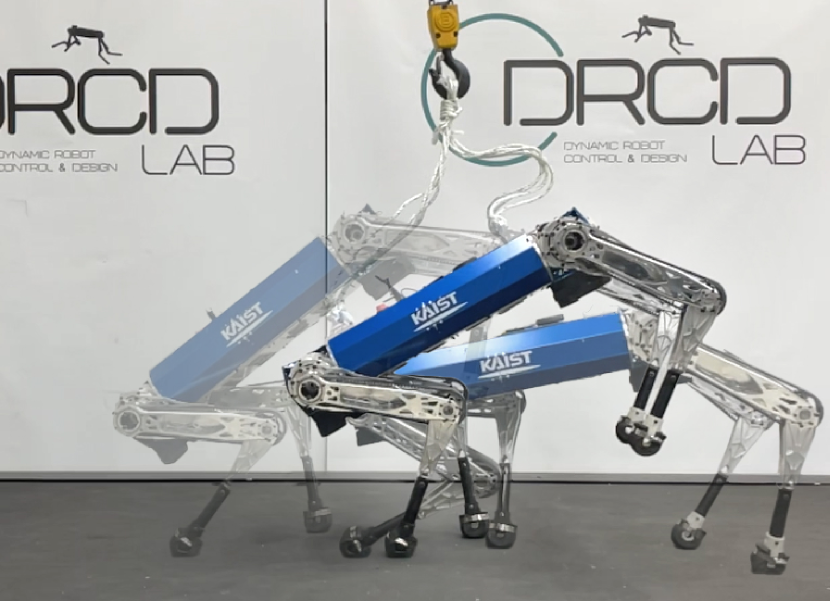
Figure 1: Experimental demonstration of front-leg rearing motion with the HOUND quadruped robot using the proposed framework. Only a desired body pitch angle was set, without any predefined contact modes.

However, previous approaches based on MPC focus on the choice of ground reaction forces or torque trajectory under the fixed contact modes, and only a few approaches consider the contact sequence (Bledt and Kim, 2019; Neunert et al., 2018). Such formulations, primarily relying on predefined contact sequences, are suited for periodic motions such as walking or running. For dynamic maneuvers demanding non-repetitive and asymmetric contact sequences, it is crucial to preset the feasible contact modes prior to optimization. However, tackling this is intricate, given the intertwined nature of overall motion patterns (e.g., body velocity, swing leg trajectory, and foothold position) with specific contact modes. Moreover, this predefined process for the entire trajectory horizon should be repeated for each distinct task.

To address the aforementioned challenges, this work employs a contact-implicit approach. This approach facilitates the concurrent discovery of feasible contact modes, ensuring compatibility with states, control inputs, and contact forces. Based on the direct transcription method (Posa et al., 2014; Manchester et al., 2019), it is necessary to incorporate the complementarity constraints resulting from the Signorini condition into an explicit constraint form to ensure the contact motion’s feasibility. However, this results in a challenging formulation within the mathematical program with complementarity constraints (MPCC). Additionally, addressing it through mixed integer programming introduces significant computational load due to the exponential combinations of contact modes. In order to avoid this computational burden, this work adopts a contact-implicit approach based on the shooting method (Tassa et al., 2012; Neunert et al., 2017; Carius et al., 2018). The complementarity constraints are considered implicitly within the optimization process; this approach mitigates the computational burden associated with the exponential increase in mode sequences as the number of contact points increases (Carius et al., 2018). Moreover, the utilization of differential dynamic programming (DDP) in solving the optimization problem, which exhibits a linear increase in computation over the horizon, enables real-time computation for contact-implicit model predictive control.

By incorporating the hard contact model into the DDP framework, the online discovery of new contact modes becomes possible. However, as outlined in Werling et al. (2021), the optimizer is easily stuck to the initial contact condition, even when alternative contact modes could lead to a reduced total cost. These challenges arise from the strict linear complementarity constraint. Specifically, this constraint inherently preserves the contact state; for instance, in the contact case, the gradient directs towards maintaining zero contact velocity, thereby preventing contact breakage. To tackle this problem, we propose an analytical gradient based on relaxed complementarity constraints. As a result, the optimizer with the proposed gradient could achieve lower-cost solutions by facilitating the discovery of new contact modes, outperforming non-relaxed scenarios.

While the exploration of diverse contact modes enriches the motion repertoire, it does not necessarily guarantee real-world robot implementation. Absent explicit considerations for foot trajectory, resultant motions often manifest insufficient foot clearance, leading to issues such as minimal foot-lifting (Posa et al., 2014) or prevalent scuffing (Carius et al., 2019). Additionally, the broader search space across various contact modes might produce undesired results, such as the three-leg walking motion of a quadruped robot. To refine these motions for practical use, we introduce differentiable cost terms designed to improve foot clearance, minimize foot slippage, and produce gait patterns without relying on periodic cost inputs.

Lastly, leveraging the MPC scheme within the proposed framework facilitates the simultaneous generation and execution of multi-contact motions. Each optimization is initialized using the prior solution trajectory for a consistent motion plan across subsequent MPC problems. However, the hybrid dynamics of the hard contact model lead to unstable initialization in the single shooting method, where the initialization relies solely on control input trajectories. This hybrid dynamics can induce numerous deviations in contact modes throughout the motion plan, even from slight initial state discrepancies (Posa et al., 2014). To address this, we utilize the multiple shooting variant of DDP. This ensures a consistent motion plan despite initial state discrepancies by enhancing robustness with initialization using state-control trajectories.

The main contributions of the paper are as follows:

• We introduce a contact-implicit MPC framework that simultaneously generates and executes diverse multi-contact motions, all without pre-planned trajectories or contact mode sequences.

• A novel analytical gradient for contact impulses, based on relaxed complementarity constraint, is proposed for promoting the discovery of new contact modes.

• For real-world implementations, we introduce specific details, including the integration of additional cost terms to ensure reliable motion and the use of the multiple shooting variant of DDP to enhance robustness.

• This approach is demonstrated through 3D simulations of dynamic quadruped motions and real-world experiments on the 45kg KAIST HOUND robot (Shin et al., 2022), including a front-leg rearing motion as shown in Figure 1 (also, Extension 1).

The remainder of this paper is structured as follows: Section 2 discusses related work on trajectory optimization in contact-implicit approaches. Section 3 provides background for our framework, and Section 4 introduces a novel method for the analytical gradient of contact impulses in relaxed complementarity constraints. Section 5 provides the entire structure of the optimal control problem, while Section 6 offers implementation details of the proposed contact-implicit MPC. Finally, Section 7 presents results from simulations and experiments, concluding with a summary in Section 8.

In our earlier study (Kim et al., 2022), we introduced the preliminary version of the contact-implicit DDP framework. However, it was restricted to a 2D environment and predominantly focused on motion generation in idealized conditions, analogous to solving a trajectory optimization problem offline in a receding horizon fashion. The first novelty of this work is an expansion of the framework to 3D environments and implementation of the whole framework for real-time execution. Additionally, this study tackles the robustness challenges within the contact-implicit MPC framework, particularly in cases where the actual integrated state deviates from the predicted state. Moreover, an analysis of the effects of relaxation variables within the complementarity constraint is presented. Finally, a series of new 3D simulation outcomes and real-world experiments on a quadruped robot with onboard computations are demonstrated.

2 Related Work

2.1 Contact-implicit Approach with Direct Transcription Method

The contact-implicit approach, which incorporates contact dynamics into the direct transcription method for trajectory optimization, has been studied (Posa et al., 2014; Manchester et al., 2019; Patel et al., 2019; Moura et al., 2022). The contact impulse is treated as an optimization variable alongside state and control inputs. Therefore, the complementarity constraints are explicitly utilized for modeling the Signorini condition and Coulomb friction to enforce physically feasible contact motion. This approach formulates the problem as a mathematical program with complementarity constraints (MPCC), known for its challenging nature due to the ill-posedness of the constraints. Consequently, relaxation methods are often employed to make these constraints more tractable for convergence and exploration of mode selections (Manchester et al., 2019; Patel et al., 2019). Similarly, a penalty approach is adopted, utilizing an objective function to ensure the feasibility of the contact dynamics (Mordatch et al., 2012a, b). However, the application of relaxation or penalty methods implies the possibility of infeasible contact motions, such as the relaxation applied to the Signorini condition, allowing contact forces to act at a non-zero distance. Consequently, it becomes essential to gradually tighten the relaxation variable as convergence to ensure feasible motions. These approaches generate various multi-contact motions without a priori contact mode sequences. However, due to the computationally expensive search for multiple-contact combinations and their poor convergence properties, these methods are typically used for offline motion generations.

Currently, progress for the real-time application using the contact-implicit approach in the direct transcription method has been made for model predictive control in Cleac’h et al. (2021); Aydinoglu and Posa (2022); Aydinoglu et al. (2023). Aydinoglu and Posa (2022); Aydinoglu et al. (2023) tackle the MPCC problem using the alternating direction method of multipliers (ADMM), where the linear complementarity problem (LCP) constraints are enforced in the sub-problems within the ADMM iterations. Within these sub-problems, they handle smaller-scale mixed-integer quadratic programs (MIQP). This approach significantly reduces the complexity of the combinatorial search problems as compared to solving a singular large MIQP for the MPCC problem about the entire horizon. This approach enables real-time MPC for multi-contact systems, such as manipulation arms interacting with multiple rigid spheres, without a priori information about contact.

Cleac’h et al. (2021) enforce the contact dynamics using a time-varying LCP approximated about the reference trajectory. By utilizing a pre-computation and structure-exploiting interior point solver for this LCP, they could achieve real-time computation for contact-implicit MPC. Through the use of an interior-point method (IPM) to solve the LCP, they compute smooth gradients using the central path parameter, which relaxes the complementarity constraints. These smooth gradients offer information about other contact modes. While this approach is capable of identifying new contact modes online, it relies on a reference trajectory computed offline in a contact-implicit manner (Manchester et al., 2019). This dependency requires distinct reference trajectories for different tasks, ultimately restricting the range of achievable motion types to the capabilities of offline trajectory optimization.

2.2 Contact-implicit Approach with Differential Dynamic Programming

The integration of the contact-implicit approach with DDP-based algorithms has been explored across various studies (Tassa et al., 2012; Neunert et al., 2017; Carius et al., 2018; Chatzinikolaidis and Li, 2021; Kurtz and Lin, 2022; Kong et al., 2023). A key distinction from direct transcription methods lies in the treatment of the contact impulse, which becomes a function of both the system’s state and control input. The complementarity constraint, known for causing numerical challenges in optimization, does not appear as an explicit constraint in the optimal control problem; instead, it is integrated into the system dynamics. Therefore, in the forward pass, the contact impulse, corresponding to a specific state and control input, needs to be computed, while in the backward pass, computation of the contact impulse’s gradient is required.

The gradient of the contact impulse is commonly computed using a differentiable contact model, as in Tassa et al. (2012), to facilitate the discovery of other contact modes. To enhance the exploration of contact modes, virtual forces on potential contact points can be introduced to unveil new contacts (Önol et al., 2019, 2020). Adopting a soft contact model with a smoothing term (Todorov, 2011, 2014) enhances this procedure, which is noticeable in gradient-based method in MuJoCo MPC (Howell et al., 2022) and DDP with implicit dynamics formulation (Chatzinikolaidis and Li, 2021). Moreover, this approach can be extended to MPC scenarios, as evidenced by the simulation of humanoid getting-up and walking motions (Tassa et al., 2012). The approach exhibits near real-time performance and remarkable robustness with smoothing contact dynamics.

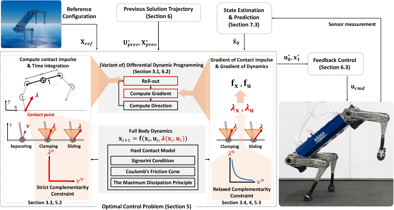
Figure 2: The overall framework of the contact-implicit model predictive control (MPC): The optimal control problem is tackled using a variant of the differential dynamic programming (DDP) algorithm, with the integration of a hard contact model within the system dynamics. The strict complementarity constraint, arising from the Signorini condition, is exclusively employed during the roll-out process, while the relaxed complementarity constraint is employed when computing the gradient component.

The contact-implicit DDP approach has begun to emerge in the context of quadruped robots and real-hardware experiments, employing the spring-damper model to ensure smooth gradients, as showcased in studies such as Neunert et al. (2017, 2018). The spring-damper model is helpful to reason about the new contact modes while losing physical realism (e.g., ground penetration or non-vanishing contact forces). The trajectory optimization method (Neunert et al., 2017) reveals diverse contact-rich motions, though versatile motion requires careful cost tuning and faces challenges in real-world transfer due to robustness issues. Integrating the contact-implicit approach with MPC enhances robustness (Neunert et al., 2018), shown through hardware experiments with trotting and squat jump motions guided by periodic cost functions. Leveraging the contact-implicit approach, the method adapts contact sequences during trot motions to handle disturbances. Although the trajectory optimization process discovers a wide range of motions, the real-world implementation remains biased toward relatively static motions such as periodic trotting and squat jump motions.

Due to the inherent issues associated with the spring-damper model in Neunert et al. (2018), such as physically unrealistic motion and requiring small time steps due to numerical stiffness, it led to the adoption of a hard contact model (Carius et al., 2018) and with a relaxation term (Carius et al., 2019). The computation of the contact impulse is achieved through quadratically constrained quadratic programming (QCQP), while gradient computation relies on automatic differentiation. The effectiveness of optimized trajectories, encompassing contact switching motions, is demonstrated through experiments involving one-leg hopper jumping (Carius et al., 2018), as well as walking and slippage motions of quadruped robots (Carius et al., 2019). However, challenges persist, particularly concerning the discovery of new contact modes and the implementation of MPC under the cases of contact mismatches (Carius et al., 2019). The utilization of a hard contact model makes the computation of gradients based on the specific roll-out contact modes, limiting exploration to other contact modes, as pointed out in prior work (Werling et al., 2021). Additionally, the employment of a single shooting method with the hard contact model renders the MPC approach initiated with previous solutions vulnerable to instability arising from minor contact mismatches during the initial roll-out.

2.2.1 Proposed Method.

Our approach is based on the contact-implicit approach with DDP, employing a hard contact model to reduce the smoothing effect to the physical constraint (e.g., force at a distance) in simulation. The hard contact model is based on the QCQP formulation with an explicit constraint of the Signorini condition as in Hwangbo et al. (2018), and the gradient of the contact impulse is analytically computed based on the approach in Werling et al. (2021). To handle the challenges of exploring new contact modes, we introduce a novel smooth gradient based on the relaxed complementarity constraints: Exact simulation (no relaxation) in the forward pass and smooth gradient (with relaxation) in the backward pass, as depicted in the overview of the entire framework in Figure 2. The problem of the unstable initial roll-out in the MPC setting is addressed by leveraging Feasibility-driven Differential Dynamic Programming (FDDP) (Mastalli et al., 2020), which is a multiple shooting variant of DDP. Additionally, we incorporate extra cost terms to enhance motion reliability, mitigating issues such as scuffing motion found in Carius et al. (2019).

3 Background

This section outlines the theoretical background of our framework. The optimal control problem is tackled using a DDP-based algorithm. To address the unstable initialization problem, FDDP, a multiple-shooting variant of DDP, is employed. Consequently, a brief introduction to both DDP and its variant, FDDP, is provided. This section then presents the notation used for full body dynamics and contact dynamics. Given the contact-implicit DDP framework, it is required to compute the contact impulse for state integration in the DDP forward pass and its gradient for the backward pass. Therefore, this section details the computation of the contact impulse and its analytical gradient.

3.1 Differential Dynamic Programming

DDP (Mayne, 1966; Tassa et al., 2012) is a direct single-shooting approach to solve a finite-horizon optimal control problem with a discrete-time dynamical system:

$$\min_{\mathbf{U}}~{} l_{N}(\mathbf{x}_{N})+\sum_{i=0}^{N-1}l(\mathbf{x}_{i},\mathbf{u}_{i})$$ (1a)

$$s.t.~{} \mathbf{x}_{i+1}=\mathbf{f}(\mathbf{x}_{i},\mathbf{u}_{i}),$$ (1b)

where $\mathbf{U}=\{\mathbf{u}_{0},\ldots,\mathbf{u}_{N-1}\}$ represents sequence of control inputs, and $l(\mathbf{x}_{i},\mathbf{u}_{i})$ and $l_{N}(\mathbf{x}_{N})$ are the running and final costs, respectively. $\mathbf{x}_{i}$ and $\mathbf{u}_{i}$ denote the state and control at time step $i$, and $\mathbf{f}$ is the generic function of dynamics.

For this optimization problem (1), the value function $V(\mathbf{x}_{i})$ could be defined as optimal cost-to-go from $\mathbf{x}_{i}$. Based on Bellman’s Optimality Principle, the following recursive relation holds: $V(\mathbf{x}_{i})=\min_{\mathbf{u}_{i}}[l(\mathbf{x}_{i},\mathbf{u}_{i})+V^{\prime}(\mathbf{f}(\mathbf{x}_{i},\mathbf{u}_{i}))]$. Introducing the action-value function, which is defined as $Q(\mathbf{x}_{i},\mathbf{u}_{i})\triangleq l(\mathbf{x}_{i},\mathbf{u}_{i})+V^{\prime}(\mathbf{f}(\mathbf{x}_{i},\mathbf{u}_{i}))$, we approximate it locally in a quadratic manner to derive the control sequence improvement. The coefficients for this quadratic approximation are as follows:

$$Q_{\mathbf{x}}=l_{\mathbf{x}}+\mathbf{f}_{\mathbf{x}}^{T}V_{\mathbf{x}}^{\prime},~{}Q_{\mathbf{u}}=l_{\mathbf{u}}+\mathbf{f}_{\mathbf{u}}^{T}V_{\mathbf{x}}^{\prime},$$ (2)

$$Q_{\mathbf{xx}}=l_{\mathbf{xx}}+\mathbf{f}_{\mathbf{x}}^{T}V_{\mathbf{xx}}^{\prime}\mathbf{f}_{\mathbf{x}}+V_{\mathbf{x}}^{\prime}\cdot\mathbf{f}_{\mathbf{xx}},$$

$$Q_{\mathbf{xu}}=l_{\mathbf{xu}}+\mathbf{f}_{\mathbf{x}}^{T}V_{\mathbf{xx}}^{\prime}\mathbf{f}_{\mathbf{u}}+V_{\mathbf{x}}^{\prime}\cdot\mathbf{f}_{\mathbf{xu}},$$

$$Q_{\mathbf{uu}}=l_{\mathbf{uu}}+\mathbf{f}_{\mathbf{u}}^{T}V_{\mathbf{xx}}^{\prime}\mathbf{f}_{\mathbf{u}}+V_{\mathbf{x}}^{\prime}\cdot\mathbf{f}_{\mathbf{uu}}.$$

The second derivative of dynamics $\mathbf{f}_{\mathbf{xx}}$, $\mathbf{f}_{\mathbf{xu}}$, and $\mathbf{f}_{\mathbf{uu}}$ are often ignored in iLQG (Tassa et al., 2012), corresponding to the Gauss-Newton Hessian approximation. In our work, these second derivative terms are not computed.

In the backward pass, minimizing the quadratic approximation of the action-value function yields the optimal control change as $\delta\mathbf{u}^{*}(\delta\mathbf{x})=\mathbf{k}+\mathbf{K}\delta\mathbf{x}$, where the feed-forward term is $\mathbf{k}\triangleq-Q_{\mathbf{uu}}^{-1}Q_{\mathbf{u}}$, and the feedback gain is $\mathbf{K}\triangleq-Q_{\mathbf{uu}}^{-1}Q_{\mathbf{ux}}$. By utilizing it, we can compute the quadratic approximation of the value function, thereby establishing a recursive relation to determine the optimal control modification across all time steps, from $N$ to 0.

In the forward pass, the states and control inputs are updated starting from the initial state $\mathbf{\tilde{x}}_{0}$, using $\mathbf{k}$ and $\mathbf{K}$ from the backward pass:

$$\mathbf{\hat{x}}_{0} =\mathbf{\tilde{x}}_{0},$$ (3)

$$\mathbf{\hat{u}}_{i} =\mathbf{u}_{i}+\alpha\mathbf{k}_{i}+\mathbf{K}_{i}(\mathbf{\hat{x}}_{i}\ominus\mathbf{x}_{i}),$$

$$\mathbf{\hat{x}}_{i+1} =\mathbf{f}(\mathbf{\hat{x}}_{i},\mathbf{\hat{u}}_{i}),$$

where $\ominus$ denotes the difference operator of the state manifold (following the notations in Mastalli et al. (2022a)), needed to optimize over the manifold (Gabay, 1982). $\alpha$ denotes the step size for backtracking line search. In practical application, regularization is also necessary. This method could be extended to accommodate box constraints on control input (Tassa et al., 2014) and address nonlinear state-control constraints (Xie et al., 2017).

3.1.1 Feasibility-driven Differential Dynamic Programming.

FDDP (Mastalli et al., 2020) is a multiple-shooting variant of DDP. It is designed to accommodate infeasible state-control trajectories for warm-start initialization and manage dynamically infeasible iterations. As a result, this method offers enhanced globalization compared to classical DDP.

FDDP accepts infeasible state-control trajectories by adapting the backward pass and opening the dynamics gaps in early iterations in the forward pass. For the infeasible state-control trajectory $\mathbf{x}_{0},...,\mathbf{x}_{N},\mathbf{u}_{0},...,\mathbf{u}_{N-1}$, where $\mathbf{x}_{i}$ represents the shooting state, the dynamics gap $\mathbf{\bar{f}}_{i}$ is determined as follows:

$$\mathbf{\bar{f}}_{0}:=\mathbf{\tilde{x}}_{0}\ominus\mathbf{x}_{0},$$ (4)

$$\mathbf{\bar{f}}_{i+1}:=\mathbf{f}(\mathbf{x}_{i},\mathbf{u}_{i})\ominus\mathbf{x}_{i+1},\quad{\scriptstyle\forall i=\{0,1,...,N-1\}},$$

where $\mathbf{\tilde{x}}_{0}$ denotes the initial state, and $\mathbf{\bar{f}}_{0},\mathbf{\bar{f}}_{i+1}$ indicate the gap in the dynamics, on the tangent space of the state manifold.

The backward pass is adapted to accept infeasible trajectories as proposed in Giftthaler et al. (2018). It adjusts the Jacobian of the value function to reflect the deflection from the gap as $V_{\mathbf{x}}^{+}=V_{\mathbf{x}}^{\prime}+V_{\mathbf{xx}}^{\prime}\mathbf{\bar{f}}_{i+1}$. Subsequently, $V_{\mathbf{x}}^{+}$ is utilized to compute (2) instead of $V_{\mathbf{x}}^{\prime}$.

In the forward pass, the nonlinear roll-out process for $\alpha$-step is given by:

$$\mathbf{\hat{x}}_{0} =\mathbf{\tilde{x}}_{0}\oplus(\alpha-1)\mathbf{\bar{f}}_{0},$$ (5)

$$\mathbf{\hat{u}}_{i} =\mathbf{u}_{i}+\alpha\mathbf{k}_{i}+\mathbf{K}_{i}(\mathbf{\hat{x}}_{i}\ominus\mathbf{x}_{i}),$$

$$\mathbf{\hat{x}}_{i+1} =\mathbf{f}(\mathbf{\hat{x}}_{i},\mathbf{\hat{u}}_{i})\oplus(\alpha-1)\mathbf{\bar{f}}_{i+1},$$

where $\oplus$ denotes the integrator operator, needed to optimize over the manifold (Gabay, 1982). This roll-out maintains an equivalent gap contraction rate for the $\alpha$-step in direct multiple shooting, given by $\mathbf{\bar{f}}_{i}\leftarrow(1-\alpha)\mathbf{\bar{f}}_{i}$. FDDP approves the trial step in an ascent direction to decrease infeasibility while slightly increasing the cost. Due to its feasibility-driven approach, FDDP exhibits a larger basin of attraction to the good local optimum than DDP (Mastalli et al., 2022a). This method has been extended to address control limits as presented in Box-FDDP (Mastalli et al., 2022a), which serves as the primary optimal control problem solver in our work.

3.2 Notation for Full Body Dynamics and Contact Dynamics

In this section, we focus our interest on the case when the discrete-time dynamic model (1b) incorporates contact dynamics. Our framework employs a velocity-based time-stepping scheme. Given contact impulse $\bm{\lambda}_{i}$, next time step’s generalized velocity $\mathbf{\dot{q}}_{i+1}\in\mathbb{R}^{n_{\dot{q}}}$ can be obtained by:

$$\mathbf{q}_{i+1}=\mathbf{q}_{i}\oplus\mathbf{\dot{q}}_{i+1}dt,$$ (6)

$$\mathbf{\dot{q}}_{i+1}=\mathbf{M}_{i}^{-1}((-\mathbf{h}_{i}+\mathbf{B}\mathbf{u}_{i})dt+\mathbf{M}_{i}\mathbf{\dot{q}}_{i}+\mathbf{J}_{i}^{T}\bm{\lambda}_{i}),$$

where generalized coordinate $\mathbf{q}_{i}\in\mathrm{SE}(3)\times\mathbb{R}^{n_{j}}$ and generalized velocity $\mathbf{\dot{q}}_{i}\in\mathfrak{se}(3)\times\mathbb{R}^{n_{j}}$, where $\mathbf{\dot{q}}_{i}$ is the tangent vector to the configuration $\mathbf{q}_{i}$ with dimension $n_{\dot{q}}$ (not the same dimension with $\mathbf{q}_{i}$). $\mathbf{u}_{i}\in\mathbb{R}^{n_{j}}$ are the joint torque, and $n_{j}$ is the number of articulated joints. $\mathbf{M}_{i}=\mathbf{M}(\mathbf{q}_{i})\in\mathbb{R}^{n_{\dot{q}}\times n_{\dot{q}}}$ is the mass matrix, $\mathbf{h}_{i}=\mathbf{h}(\mathbf{q}_{i},\mathbf{\dot{q}_{i}})\in\mathbb{R}^{n_{\dot{q}}}$ is a bias vector that includes Coriolis and gravitational terms at time step $i$, $\mathbf{B}=[\mathbf{0}_{n_{j}\times 6},\mathbf{I}_{n_{j}\times n_{j}}]^{T}\in\mathbb{R}^{n_{\dot{q}}\times n_{j}}$ is an input matrix, and $dt$ is a time step.

Here, $\bm{\lambda}_{k,i}\in\mathbb{R}^{3}$ is expressed for $k$ th contact point at time step $i$ in the contact frame (whose z-axis is parallel to the respective normal vector), thereby having normal and tangential components which are denoted by ${\lambda}^{n}_{k,i}$ and ${\bm{\lambda}}^{t}_{k,i}$, respectively. The superscripts $n$ and $t$ represent normal components and tangential components, respectively. Concatenating all contact impulses at time step $i$ gives $\bm{\lambda}_{i}=[\bm{\lambda}_{1,i}^{T},\cdots,\bm{\lambda}_{d,i}^{T}]^{T}$, where $d$ signifies the total number of contact points. Similarly, the contact Jacobian $\mathbf{J}_{i}=[\mathbf{J}_{1,i}^{T},\cdots\mathbf{J}_{d,i}^{T}]^{T}$ comprises of individual contact Jacobians for each point, with $\mathbf{J}_{k,i}\in\mathbb{R}^{3\times n_{\dot{q}}}$. The resulting contact velocity for the $k$ th point at time $i+1$ is $\mathbf{v}_{k,i+1}=\mathbf{J}_{k,i}\mathbf{\dot{q}}_{i+1}$, encompassing the contact impulse’s effect from time $i$ and split into normal $v^{n}_{k,i+1}$ and tangential $\mathbf{v}^{t}_{k,i+1}$ components.

For brevity in Sections 3.2.1, 3.3, 3.4, and 4, the subscript time index $i$ is omitted for variables such as $\mathbf{M},\mathbf{J}_{k},\mathbf{h}$, and $\bm{\lambda}_{k}$. However, for clarity, $i$ is retained for $\mathbf{\dot{q}}_{i}$ and $\mathbf{u}_{i}$. Additionally, the time index for the next time step, $i+1$, is consistently denoted (e.g., $\mathbf{v}_{k,i+1}$, $\mathbf{\dot{q}}_{i+1}$).

3.2.1 Linear Complementarity Problem (LCP).

The Signorini condition is a fundamental principle for modeling hard contact, expressed as $\phi_{k,i+1}\geq 0,\lambda_{k}^{n}\geq 0,\text{and }\phi_{k,i+1}\lambda_{k}^{n}=0$, where $\phi_{k,i+1}$ represents the height of the $k$ th foot from the ground. In this condition, the non-contacting foot, which maintains a distance from the ground, does not receive a contact impulse, while the contacting foot receives a contact impulse. For computational simplicity, the Signorini condition can be expressed in velocity space as $v^{n}_{k,i+1}\geq 0,\lambda_{k}^{n}\geq 0,\text{and }v^{n}_{k,i+1}\lambda_{k}^{n}=0$.

Given the time-stepping scheme (equation (6)), the contact velocity $\mathbf{v}_{k,i+1}$ is an affine function of the contact impulse $\bm{\lambda}_{k}$. This formulation allows the Signorini condition in velocity space to be represented as a linear complementarity constraint. Consequently, the problem of determining a feasible $v^{n}_{k,i+1}\text{ and }\lambda_{k}^{n}$ can be cast as an LCP (Cottle et al., 2009). In the following subsection, the linear complementarity constraint is utilized to compute the feasible contact impulse.

3.3 Contact Impulse

For the contact-implicit approach, the contact impulse is computed in the integration step of roll-out (3). In this work, the contact impulse $\bm{\lambda}$ is obtained with the per-contact iteration method with the hard contact model in Preclik (2014); Hwangbo et al. (2018). By applying the Signorini condition in velocity space, we initially categorize the contact scenarios. In the case of opening contact (separating), the contact impulse is zero. For the closing contact scenarios (clamping and sliding), the contact impulse for the $k$th contact point is computed by solving the following optimization problem that aims to minimize the kinetic energy at the contact point, based on the maximum dissipation principle:

$$\min_{\bm{\lambda}_{k}}{\mathbf{v}_{k,i+1}}^{T}\mathbf{M}^{\text{app}}_{k}{\mathbf{v}_{k,i+1}}$$ (7)

$$s.t.\quad\bm{\lambda}_{k}\in{\cal{S}}_{k},$$

where $\mathbf{M}^{\text{app}}_{k}:=(\mathbf{J}_{k}\mathbf{M}^{-1}\mathbf{J}_{k}^{T})^{-1}$ is the apparent inertia matrix at the contact point. Given that $\tilde{\mathbf{k}}$ denotes all the contact indices only except $k$, the contact velocity of the contact point $k$ can be obtained by:

$$\mathbf{v}_{k,i+1}=\mathbf{c}_{k}+(\mathbf{M}^{\text{app}}_{k})^{-1}\bm{\lambda}_{k},$$ (8)

where $\mathbf{c}_{k}:=\mathbf{J}_{k}\mathbf{M}^{-1}((-\mathbf{h}+\mathbf{B}\mathbf{u}_{i})dt+\mathbf{J}_{\tilde{\mathbf{k}}}^{T}\bm{\lambda}_{\tilde{\mathbf{k}}}+\mathbf{M}\mathbf{\dot{q}}_{i})$. The feasible set ${\cal{S}}_{k}$ is formed by the following two conditions:

$$v^{n}_{k,i+1}\geq 0,\lambda_{k}^{n} \geq 0,\text{and }v^{n}_{k,i+1}\lambda_{k}^{n}=0,$$ (9a)

$${\|\bm{\lambda}}^{t}_{k}\| \leq\mu\lambda^{n}_{k},$$ (9b)

where $\mu$ is the friction coefficient. The first constraint (9a) arises from the Signorini condition, while the second condition (9b) represents Coulomb’s friction cone constraint. Currently addressing closing contact scenarios (clamping and sliding), the condition (9a) simplifies to an affine condition as $v^{n}_{k,i+1}=0$. In the clamping case, the optimal solution is $\bm{\lambda}_{k}=-\mathbf{M}_{k}\mathbf{c}_{k}$. For the sliding case, the optimization problem (7) is formulated to QCQP (Lidec et al., 2023) and can be solved by utilizing the bisection method as proposed in Hwangbo et al. (2018).

In scenarios with multiple contacts, the contact impulses $\bm{\lambda}_{1},\cdots,\bm{\lambda}_{d}$ of all the contact points can be obtained by solving the multiple instances of the optimization problem (7) for all $k=1,\cdots,d$. Because the multiple instances of the optimization problem are not independent of each other due to the term $\bm{\lambda}_{\tilde{\mathbf{k}}}$, the nonlinear block Gauss-Seidel method is employed in Hwangbo et al. (2018) to solve this problem iteratively.

3.4 Analytical Gradient of Contact Impulse

To compute $\mathbf{f}_{\mathbf{x}}$ and $\mathbf{f}_{\mathbf{u}}$, specifically the derivatives of the dynamics with respect to $\mathbf{x}$ and $\mathbf{u}$ (utilized in the backward pass as detailed in (2)), the gradient of the contact impulse is required. Based on the method in Werling et al. (2021), the analytical gradient of the contact impulse is computed efficiently by leveraging the sparsity derived from the complementarity constraints. Because the contact impulse is obtained from the constrained optimization (7), different types of the solution can exist due to the Signorini condition and Coulomb’s friction constraint. The solution of contact impulse can be categorized into three types according to the value of $\bm{\lambda}_{k}$ and $\mathbf{v}_{k,i+1}$ as shown in Figure 3.

3.4.1 Separating.

If $\bm{\lambda}_{k}=\bm{0}$, then the contact velocity $\mathbf{v}_{k,i+1}=\mathbf{c}_{k}$ according to (8). The gradient of $\frac{\partial{\bm{\lambda}}_{k}}{\partial\xi}$ will be zero for an arbitrary variable $\xi$ because $\bm{\lambda}_{k}=\bm{0}$.

3.4.2 Clamping.

In this case, with ${v}^{n}_{k,i+1}=0$ and $\mathbf{v}^{t}_{k,i+1}={0}$, the contact point remains contact with the ground and does not slide in the tangential direction at the next time step. Then, the gradient of $\frac{\partial\bm{\lambda}_{k}}{\partial\xi}$ has to be obtained considering the constraints $\mathbf{v}_{k,i+1}=0$.

3.4.3 Sliding.

In this last case, given ${v}^{n}_{k,i+1}=0$, the contact point remains contact with the ground, though the tangential velocity $\mathbf{v}^{t}_{k,i+1}$ can vary. The contact impulse exists on the boundary of the friction cone and then be expressed as $\bm{\lambda}_{k}=\mathbf{E}_{k}{\lambda^{n}_{k}}$, where the matrix $\mathbf{E}_{k}=[\mu cos(\theta_{k}),\mu sin(\theta_{k}),1]^{T}$ is determined through the optimization problem in (7). Then, the gradient of $\frac{\partial\bm{\lambda}_{k}}{\partial\xi}$ has to be obtained considering the constraints ${v}^{n}_{k,i+1}=0$ and $\bm{\lambda}_{k}=\mathbf{E}_{k}{\lambda^{n}_{k}}$.

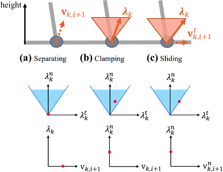
Figure 3: Illustration of a contact impulse and contact velocity in the cases of (a) Separating, (b) Clamping, and (c) Sliding

The following provides a methodology to compute $\frac{\partial\bm{\lambda}_{k}}{\partial\xi}$ for clamping and sliding scenarios. Let $\mathbf{c}$ denote the set of indices for clamping contact points and $\mathbf{s}$ for sliding contact points. With this set notation, any variable $\mathbf{y}$ with the subscript $\mathbf{c}$ or $\mathbf{s}$ will denote a vector or matrix constructed by vertically concatenating $\mathbf{y}_{c}$ or $\mathbf{y}_{s}$ for all $c\in\mathbf{c}$ or $s\in\mathbf{s}$. For example, given $\mathbf{c}=\{1,3\}$, the corresponding contact Jacobian becomes $\mathbf{J}_{\mathbf{c}}=\left[\mathbf{J}_{1}^{T},~{}\mathbf{J}_{3}^{T}\right]^{T}$ and corresponding contact velocity becomes $\mathbf{v}_{\mathbf{c},i+1}=\left[{\mathbf{v}_{1,i+1}}^{T},~{}{\mathbf{v}_{3,i+1}}^{T}\right]^{T}$. Only for the matrix $\mathbf{E}_{k}$ in the sliding contact cases, the matrix $\mathbf{E}_{\mathbf{s}}$ is a block diagonal matrix with top-left entry $\mathbf{E}_{s_{1}}$ and bottom-right entry $\mathbf{E}_{s_{n}}$, where $s_{1}$ and $s_{n}$ are the first and last elements of set $\mathbf{s}$, respectively.

Then, for clamping and sliding contact points, the following algebraic equations should hold:

$$\mathbf{v}_{\mathbf{c},i+1}=\mathbf{0},$$ (10)

$$\mathbf{v}^{n}_{\mathbf{s},i+1}=\mathbf{0}.$$

In the given context, $\mathbf{v}_{\mathbf{c},i+1}$ is a vector from the space $\mathbb{R}^{3n_{\mathbf{c}}}$, and $\mathbf{v}^{n}_{\mathbf{s},i+1}$ is from the space $\mathbb{R}^{n_{\mathbf{s}}}$, where $n_{\mathbf{c}}$ and $n_{\mathbf{s}}$ represent the number of clamping points and sliding points, respectively.

The above equation (10) can be rewritten so that the contact impulse $\bm{\lambda}$ is explicitly shown in the equation. First, the next step’s velocity $\mathbf{\dot{q}}_{i+1}$ is obtained in the manner that contact impulse is decomposed into clamping and sliding cases as follows,

$$\mathbf{\dot{q}}_{i+1}=\mathbf{M}^{-1}((-\mathbf{h}+\mathbf{B}\mathbf{u}_{i})dt+\mathbf{M}\mathbf{\dot{q}}_{i}+{\mathbf{J}_{\mathbf{c}}}^{T}\bm{\lambda}_{\mathbf{c}}+{\mathbf{J}_{\mathbf{s}}}^{T}\bm{\lambda}_{\mathbf{s}}),$$

because, in the case of sliding, $\bm{\lambda}_{\mathbf{s}}=\mathbf{E}_{\mathbf{s}}{\bm{\lambda}^{n}_{\mathbf{s}}}$,

$$\mathbf{\dot{q}}_{i+1}=\mathbf{M}^{-1}((-\mathbf{h}+\mathbf{B}\mathbf{u}_{i})dt+\mathbf{M}\mathbf{\dot{q}}_{i}+{\mathbf{J}_{\mathbf{c}}}^{T}\bm{\lambda}_{\mathbf{c}}+{\mathbf{J}_{\mathbf{s}}}^{T}\mathbf{E}_{\mathbf{s}}\bm{\lambda}^{n}_{\mathbf{s}}).$$

Identifying $\mathbf{v}_{\mathbf{c},i+1}=\mathbf{J}_{\mathbf{c}}\mathbf{\dot{q}}_{i+1}$ and $\mathbf{v}^{n}_{\mathbf{s},i+1}=\mathbf{J}^{n}_{\mathbf{s}}\mathbf{\dot{q}}_{i+1}$, and then vertically concatenating two equations of (10), we can rewrite (10) as,

$$\mathbf{0}=\mathbf{A}\bm{\lambda}^{\text{contact}}+\mathbf{b},$$ (11)

where,

$$\bm{\lambda} {}^{\text{contact}}=\begin{bmatrix}{\bm{\lambda}_{\mathbf{c}}}^{T}&{\bm{\lambda}^{n}_{\mathbf{s}}}^{T}\end{bmatrix}^{T},$$

$$\mathbf{A} =\begin{bmatrix}\mathbf{J}_{\mathbf{c}}\\ \mathbf{J}^{n}_{\mathbf{s}}\end{bmatrix}\mathbf{M}^{-1}\begin{bmatrix}\mathbf{J}_{\mathbf{c}}\\ \mathbf{E}_{\mathbf{s}}^{T}{\mathbf{J}_{\mathbf{s}}}\end{bmatrix}^{T},$$

$$\mathbf{b} =\begin{bmatrix}\mathbf{J}_{\mathbf{c}}\\ \mathbf{J}^{n}_{\mathbf{s}}\end{bmatrix}\mathbf{M}^{-1}\left((-\mathbf{h}+\mathbf{B}\mathbf{u}_{i})dt+\mathbf{M}\mathbf{\dot{q}}_{i}\right),$$

where $\mathbf{A}$ represents the Delassus matrix, and $\mathbf{b}$ denotes the contact velocity of the unconstrained motion, excluding the influence of contact impulses.

With (11), the contact impulse $\bm{\lambda}^{\text{contact}}$ is represented as,

$$\bm{\lambda}^{\text{contact}}=-\mathbf{A}^{-1}\mathbf{b}.$$ (12)

Then, the gradient of $\bm{\lambda}^{\text{contact}}$ with respect to $\xi$ is obtained:

$$\frac{\partial\bm{\lambda}^{\text{contact}}}{\partial\xi}=\mathbf{A}^{-1}\frac{\partial\mathbf{A}}{\partial\xi}\mathbf{A}^{-1}\mathbf{b}-\mathbf{A}^{-1}\frac{\partial\mathbf{b}}{\partial\xi}.$$ (13)

Furthermore, utilizing $\bm{\lambda}_{\mathbf{s}}=\mathbf{E}_{\mathbf{s}}{\bm{\lambda}^{n}_{\mathbf{s}}}$, the gradient of $\bm{\lambda}_{\mathbf{s}}$ including tangential direction can be obtained by,

$$\frac{\partial\bm{\lambda}_{\mathbf{s}}}{\partial\xi}=\mathbf{E}_{\mathbf{s}}\frac{\partial\bm{\lambda}^{n}_{\mathbf{s}}}{\partial\xi}.$$ (14)

Equations (13) and (14) are used to obtain $\frac{\partial\bm{\lambda}}{\partial\mathbf{q}_{i}}$, $\frac{\partial\bm{\lambda}}{\partial\mathbf{\dot{q}}_{i}}$, and $\frac{\partial\bm{\lambda}}{\partial\mathbf{u}_{i}}$.

4 Analytical Gradient based on Relaxed Complementarity Constraints

4.1 Problem Statement

The analytical gradient computation described in Section 3.4 achieves computational efficiency, attributed to the concise linear equation (12) it addresses. Nevertheless, there are circumstances where the application of this gradient might hinder the optimization from achieving optimal solutions, as highlighted in Werling et al. (2021). In this context, the analytical gradient is computed based on established contact modes during the roll-out process, governed by the hard contact model. Since the gradient is computed in a local region that preserves the contact state, it offers limited information to guide other contact modes.

For clamping cases, the gradient is computed for the local region where $v^{n}_{k,i+1}=0$, thereby directing towards maintaining a zero contact velocity. As a result, relying on this search direction inhibits motions for breaking of contact to reduce associated costs. For example, if the optimizer is initialized with a fully-contacted state, such as a standing motion for a quadruped, it tends to retain this contact state and converges to a fully-contacted motion. Consequently, cost reduction becomes restricted when further cost decrease requires actions involving contact breakage, such as when the reference configuration is significantly far from the robot, requiring maneuvers such as jumping.

The same holds true for separating cases. However, while the gradient encourages a zero contact impulse, gravitational effects present opportunities for making new contact instances. For instance, a falling robot without any active control would eventually establish contact, resulting in the emergence of new contacts during the roll-out process. This is also pointed out in Tassa and Todorov (2010). However, for the clamping scenarios, there is no inherent force that guides the system towards breaking the contact.

The lack of information in the gradient to the direction of breaking contact can be alleviated by relaxing the bilinear condition ${v}^{n}_{k,i+1}\lambda^{n}_{k}=0$ to the modified complementarity condition with ${v}^{n}_{k,i+1}\lambda^{n}_{k}=\rho$ for some small $\rho\geq 0$ as shown in Figure 4. This allows the solutions to move along the smooth curve ${v}^{n}_{k,i+1}{\lambda}^{n}_{k}=\rho$ during iterations rather than to stick to either ${v}^{n}_{k,i+1}=0$ or ${\lambda}^{n}_{k}={0}$. Furthermore, it aids optimization algorithms in bypassing numerical challenges arising in the vicinity of ${v}^{n}_{k,i+1}=0$ and $\lambda^{n}_{k}=0$, where there is uncertainty over whether a solution adheres to ${v}^{n}_{k,i+1}=0$ or ${\lambda}^{n}_{k}=0$. Such relaxation strategies have found successful applications across various optimization algorithms for trajectory optimization (Manchester et al., 2019; Patel et al., 2019) and quadratic programming (Pandala et al., 2019).

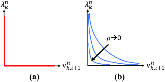
Figure 4: Illustration of (a) a Complementarity condition and (b) relaxed Complementarity condition with the parameter $\rho$

To integrate this relaxation into the DDP-based algorithm, we propose the analytical gradient of contact impulse based on the relaxed complementarity constraint. Distinct from other studies (Manchester et al., 2019; Patel et al., 2019; Mordatch et al., 2012b) that relax the physical constraint during the optimization process, requiring the relaxation to reduce to zero through iterations for feasibility, our method employs this relaxed gradient only in the backward pass. The forward roll-out is governed by a strict complementarity constraint. Therefore, this approach ensures that the trajectory is always feasible (i.e., satisfies modeled dynamics), even before convergence in the single shooting scheme. Using the relaxed gradient, the optimizer can explore motions with contact breakage, transitioning from the initial contacted state to achieve refined solutions. The impact of this relaxation is further discussed in the Section 7.

4.2 Gradient based on Relaxed Condition

Aligning with the equation (11), the linear relationship between contact velocity and contact impulse is expressed as:

$$\mathbf{v}^{\text{contact}}_{i+1}=\mathbf{A}\bm{\lambda}^{\text{contact}}+\mathbf{b},$$ (15)

where, $\mathbf{v}^{\text{contact}}_{i+1}=\left[{\mathbf{v}_{\mathbf{c},i+1}}^{T},~{}{\mathbf{v}^{n}_{\mathbf{s},i+1}}^{T}\right]^{T}$ of (10) and $\bm{\lambda}^{\text{contact}}=\begin{bmatrix}{\bm{\lambda}_{\mathbf{c}}}^{T},~{}{\bm{\lambda}^{n}_{\mathbf{s}}}^{T}\end{bmatrix}^{T}$ of (11). For the normal velocities $\mathbf{v}^{n}_{\mathbf{c},i+1}$ and $\mathbf{v}^{n}_{\mathbf{s},i+1}$, complemetarity conditions are written as,

$${v}[l]\geq 0,{\lambda}[l]\geq 0,~{}\text{and}~{}{v}[l]\lambda[l]=0,\quad{\scriptstyle\forall l\in\mathcal{N}},$$

where ${v}[l]$ and $\lambda[l]$ are the $l$ th component of vectors $\mathbf{v}^{\text{contact}}_{i+1}$ and $\bm{\lambda}^{\text{contact}}$, respectively, where $l\in\mathcal{N}$ with $\mathcal{N}$ representing the set of indices corresponding to the normal direction components. The constraints can be relaxed using a relaxation parameter $\rho>0$:

$${v}[l]>0,{\lambda}[l]>0,~{}\text{and}~{}{v}[l]\lambda[l]=\rho,\quad{\scriptstyle\forall l\in\mathcal{N}}.$$

Then each $l$ th row of (15) can be rewritten as follows,

$$\frac{\rho}{\lambda[l]}=\mathbf{a}_{l}^{T}\bm{\lambda}^{\text{contact}}+b_{l},\quad{\scriptstyle\forall l\in\mathcal{N}},$$ (16a)

where $\mathbf{a}_{l}^{T}$ is the $l$ th row of matrix $\mathbf{A}$, and $b_{l}$ is the $l$ th component of vector $\mathbf{b}$.

Differentiating this with respect to an arbitrary variable $\xi$ gives the implicit relation of $\frac{\partial\bm{\lambda}^{\text{contact}}}{\partial\xi}$ and $\bm{\lambda}^{\text{contact}}$:

$$-\frac{\rho}{\lambda[l]^{2}} (\mathbf{e}_{l}^{T}\frac{\partial\bm{\lambda}^{\text{contact}}}{\partial\xi})$$

$$= \frac{\partial\mathbf{a}_{l}^{T}}{\partial\xi}\bm{\lambda}^{\text{contact}}+\mathbf{a}_{l}^{T}\frac{\partial\bm{\lambda}^{\text{contact}}}{\partial\xi}+\frac{\partial b_{l}}{\partial\xi},\quad{\scriptstyle\forall l\in\mathcal{N}},$$ (17)

where $\mathbf{e}_{l}$ is the $l$ th elementary vector. Then, a system of linear equations is obtained:

$$\begin{bmatrix}...\\ \mathbf{a}_{l}^{T}+\frac{\rho}{\lambda[l]^{2}}\mathbf{e}_{l}^{T}\\ ...\end{bmatrix}\frac{\partial\bm{\lambda}^{\text{contact}}}{\partial\xi}+\begin{bmatrix}...\\ \frac{\partial\mathbf{a}_{l}^{T}}{\partial\xi}\bm{\lambda}^{\text{contact}}+\frac{\partial b_{l}}{\partial\xi}\\ ...\end{bmatrix}=\mathbf{0}.$$ (18)

In the case of tangential velocities, which are not subject to relaxation, the relation in (18) still holds with $\rho=0$, by (12) and (13).

Finally, we derive a simplified gradient equation:

$$\frac{\partial\bm{\lambda}^{\text{contact}}}{\partial\xi}=-[\mathbf{A}+\rho\mathbf{D}]^{-1}(\frac{\partial\mathbf{A}}{\partial\xi}\bm{\lambda}^{\text{contact}}+\frac{\partial\mathbf{b}}{\partial\xi}),$$ (19)

where $\mathbf{D}$ is the diagonal matrix which has $l$ th diagonal element as $\frac{1}{\lambda[l]^{2}}$ if $l\in\mathcal{N}$, and 0 otherwise. It is noteworthy that when $\rho=0$, the derived gradient $\frac{\partial\bm{\lambda}^{\text{contact}}}{\partial\xi}$ in (19) is identical to the gradient computed based on the strict constraint as expressed in (13).

This relaxed version of the gradient $\frac{\partial\bm{\lambda}^{\text{contact}}}{\partial\xi}$ is applied instead of (13) to obtain the gradients of the contact impulse $\frac{\partial\bm{\lambda}}{\partial\mathbf{q}_{i}}$, $\frac{\partial\bm{\lambda}}{\partial\mathbf{\dot{q}}_{i}}$, and $\frac{\partial\bm{\lambda}}{\partial\mathbf{u}_{i}}$.

5 Contact-implicit Model Predictive Control

The legged robot’s motion is generated through contact-implicit DDP framework that integrates full-body robot dynamics with contact dynamics. The optimal control problem for the 3D case is solved through Box-FDDP in Crocoddyl’s solver (Mastalli et al., 2020), and the 2D case problem is solved through constrained DDP implemented in the codebase for DDP, published in Tassa (2015). For the computation of the dynamics and its analytical derivatives, we use Pinocchio library (Carpentier et al., 2019; Carpentier and Mansard, 2018).

The feasibility of the contact impulse is ensured by applying the contact constraints (Signorini condition, Coulomb’s friction cone, and the maximum dissipation principle) for each potential contact point, $\forall k\in\{1,2,\cdots,d\}$. This framework is applied for a quadruped robot that has a single contact point per foot, $d=4$. We model each foot contact as a point contact, rather than a surface contact. Our system dynamics, $\mathbf{x}_{i+1}=\mathbf{f}(\mathbf{x}_{i},\mathbf{u}_{i})$, embeds these contact constraints during both forward roll-out and the backward pass gradient computation. Therefore, when solving the optimal control problem within DDP, the recursive QP problems do not handle these constraints as explicit constraints.

In all experiments and 3D simulations using the HOUND quadruped robot, the optimal control problem is discretized with a time step of $dt=25\,\text{ms}$, has a horizon of $N=20$, and runs in an MPC fashion at 40 Hz.

5.1 Cost

In this paper, four types of costs are utilized, with the main focus being on the regulation cost. The regulating cost alone is sufficient to generate multi-contact motion. To ensure tractable motion, three additional costs are introduced: foot slip and clearance cost, air time cost, and symmetric control cost. The regulating cost and foot slip and clearance cost are applied universally in 3D simulations and experiments, while the air time cost and symmetric control cost are specifically utilized for encouraging symmetric gaits.

The running cost $l(\mathbf{x}_{i},\mathbf{u}_{i})$ at time step $i$ consists of regulating cost $l_{r}(\mathbf{x}_{i},\mathbf{u}_{i})$, foot slip and clearance cost $l_{f}(\mathbf{x}_{i},\mathbf{u}_{i})$, air time cost $l_{a}(\mathbf{x}_{i})$, and symmetric control cost $l_{s}(\mathbf{u}_{i})$. The final cost $l_{N}(\mathbf{x}_{N})$ only includes the regulating cost:

$$l(\mathbf{x}_{i},\mathbf{u}_{i})=l_{r}(\mathbf{x}_{i},\mathbf{u}_{i})+l_{f}(\mathbf{x}_{i})+l_{a}(\mathbf{x}_{i})+l_{s}(\mathbf{u}_{i}),$$ (20)

$$l_{N}(\mathbf{x}_{N})=l_{r,N}(\mathbf{x}_{N}),$$

where $\mathbf{x}_{i}=(\mathbf{q}_{i},\mathbf{\dot{q}}_{i})$ is the robot state and $\mathbf{u}_{i}\in\mathbb{R}^{n_{j}}$ is the control input, specifically the joint torque, at time step $i$.

5.1.1 Regulating Cost.

The regulating cost is formulated as a quadratic form to minimize the error between the desired configuration and the robot’s actual configuration, as well as the error between the reference control input and the current control input:

$$l_{r}(\mathbf{x}_{i},\mathbf{u}_{i})=\|\epsilon_{\mathbf{x}_{i}}\|_{\mathbf{W}_{\mathbf{x}}}^{2}+\|\mathbf{u}_{i}-\mathbf{u}_{i,\text{ref}}\|_{\mathbf{W}_{\mathbf{u}}}^{2},$$ (21)

$$l_{r,N}(\mathbf{x}_{N})=\|\epsilon_{\mathbf{x}_{N}}\|_{\mathbf{W}_{\mathbf{x}_{N}}}^{2},$$

where $\epsilon_{\mathbf{x}_{i}}:=\mathbf{x}_{i}\ominus\mathbf{x}_{i,\text{ref}}$ is defined to include the $\mathrm{SO}(3)$ error, where the body rotational error is defined as $\epsilon_{\mathbf{R}_{i}}:=\text{log}(\mathbf{R}_{i,\text{ref}}^{T}\mathbf{R}_{i})^{\vee}$ using the logarithm map and the $vee$ operator. We use the inverse of right-Jacobian for exponential coordinates to get the Jacobian of $\epsilon_{\mathbf{R}_{i}}$ as described in Hong et al. (2020). For the remaining state components, including translation, joint configuration, and generalized velocity, the error is defined as the difference between the actual state and the desired state. Here, $\mathbf{W}_{\mathbf{x}}$ and $\mathbf{W}_{\mathbf{u}}$ are the corresponding diagonal weight matrices of the states and the control inputs, and the weight matrix for final state is defined as $\mathbf{W}_{\mathbf{x}_{N}}=\beta\mathbf{W}_{\mathbf{x}}$, where $\beta$ is a scalar weight for the final state.

5.1.2 Reference Trajectory.

In all experiments and 3D simulations with the quadruped robot, we set the reference body’s position and orientation in $\mathrm{SE}(3)$ to define the reference state $\mathbf{x}_{i,\text{ref}}=(\mathbf{q}_{i,\text{ref}},\mathbf{\dot{q}}_{i,\text{ref}})$. For instance, we adjusted the desired height or orientation, or applied a positional offset based on the robot’s current position. This choice of body reference is utilized for all the robot motions in this paper. All other components, except for the body reference, are left at zero or in their fixed nominal configurations. Both $\mathbf{\dot{q}}_{i,\text{ref}}$ and $\mathbf{u}_{i,\text{ref}}$ are set to zero, regulating deviations in $\mathbf{\dot{q}}_{i}$ and $\mathbf{u}_{i}$, respectively. The joint component of $\mathbf{q}_{i,\text{ref}}$ remains fixed as the nominal stance configuration across all tasks; leg movements are regulated based on this nominal configuration. It means that there are no pre-planned references for leg trajectories or foothold positions.

We do not interpolate reference states for smooth motion transitions; instead, the $\mathbf{x}_{i,\text{ref}}$ remains consistent for all $i\in\{0,1,\cdots,N\}$. Therefore, fixed, elementary reference trajectories are used throughout the entire horizon, showcasing the framework’s capability to handle such references.

5.1.3 Foot Slip and Clearance Cost.

In the absence of pre-planned references for leg trajectories or foothold positions, the use of only the regulating cost does not provide any improvement of cost for lifting the foot higher or avoiding slipping motion. This can result in motion lacking foot lifting and involving significant slippage, leading to challenges in real-world tracking and potential failures. To deal with this problem, we add a foot slip and clearance cost, inspired by the foot slip cost and foot clearance cost commonly used in reinforcement learning framework (Hwangbo et al., 2019; Ji et al., 2022). We formulate the individual costs as a single differentiable cost function:

$$l_{f}(\mathbf{x}_{i})=c_{f}\sum_{k=1}^{4}S(c_{1}\phi_{k,i})||\mathbf{v}_{k,i}^{t}||^{2},$$ (22)

where $S(c_{1}\phi_{k,i})=1/(1+e^{(-c_{1}\phi_{k,i})})$ is the Sigmoid function to map the foot height as a scalar weight, and $\phi_{k,i}$ and $\mathbf{v}_{k,i}^{t}$ denote the $k$ th foot height from the ground and the tangential foot velocity at time step $i$, respectively. $c_{1}$ is a tuning parameter for the steepness of the Sigmoid function, and $c_{f}$ is the total weight of the foot slip and clearance cost (set to $1$). In this paper, we assign a negative value to $c_{1}$ (set to $-30$), where this leads to specific characteristics in the function $S(c_{1}\phi_{k,i})$: it approaches a value of 0.5 for small foot heights ($\phi_{k,i}\approx 0$), and tends towards zero as the foot height $\phi_{k,i}$ increases. As a result, the tangential foot velocity is penalized when the foot is close to the ground (preventing foot slip), and the foot height is encouraged high enough when the foot has tangential velocity (ensuring foot clearance), as shown in Figure 5.

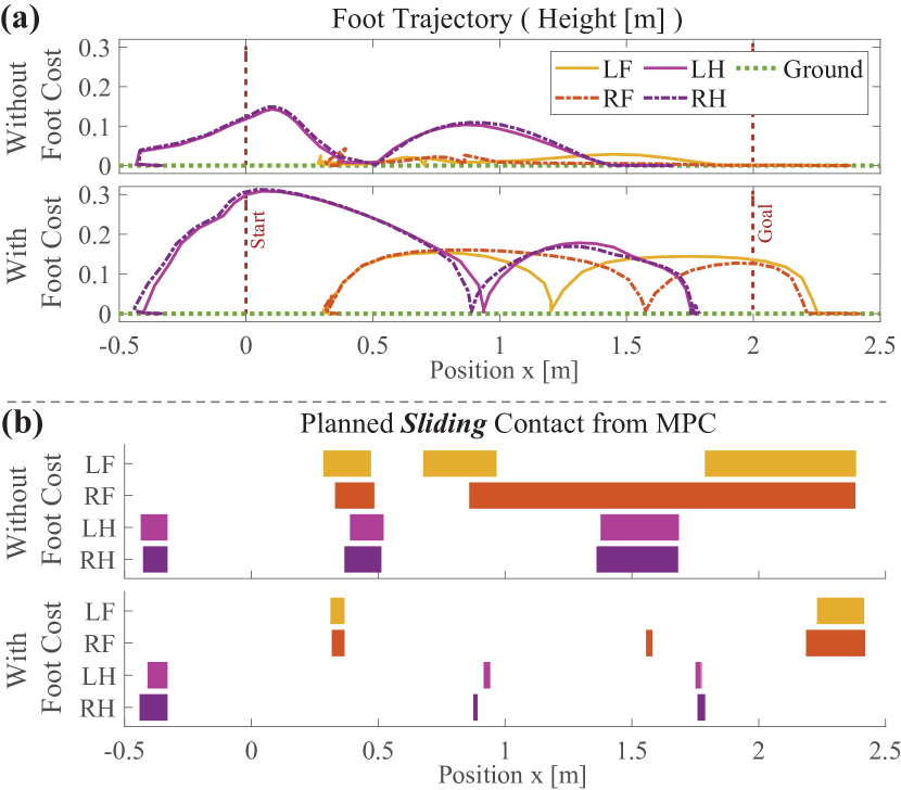
Figure 5: The effect of foot slip and clearance cost is depicted. Two scenarios are considered: ”With Foot Cost”, incorporating both regulating cost and foot slip and clearance cost, and ”Without Foot Cost”, using only the regulating cost. For both cases, the target position is set 2.0 m ahead of the initial position. The resultant swing leg trajectory is depicted in (a), and the planned sliding contact is illustrated in (b).

5.1.4 Air Time Cost.

Considering various contact points over the horizon, there could be multiple contact modes to track a specific reference configuration. Thus, a quadruped could reach its target position using fewer than four legs, such as walking with only three legs. Specific gaits, such as trotting, often require fine-tuning of weights to balance body motion, joint motion, and control input (Neunert et al., 2017). In our work, we introduce an air time cost that penalizes prolonged swing leg time during walking. This approach encourages the use of all four legs without requiring highly fine-tuned parameters for specific gaits:

$$l_{a}(\mathbf{x}_{i})=\sum_{k=1}^{4}{c_{a}}[k,i]\phi_{k,i}^{2},$$ (23)

where ${c_{a}}[k,i]$ denotes the scalar weight of the air time cost for the $k$ th contact point at time step $i$. All ${c_{a}}[k,i]$ values are initialized to 0, and are activated as a positive weight $c_{a}$ only when swing leg time surpasses threshold $i_{t}=12$ ($0.3~{}\text{sec}$). Here, the constant $c_{a}$ is set to $2\times 10^{3}$. Before solving the MPC problem at each time step, we check on the initial trajectory to identify which leg has excessive swing time over the entire horizon. For the identified leg, ${c_{a}}[k,i]$ is set to positive weight $c_{a}$ for time steps $i_{t}$ to $i_{t}+3$, penalizing foot lift with the term $\phi_{k,i}^{2}$. Once activated, this weight persists and propagates in subsequent MPC problems until it reaches the end of the horizon (time step $0$).

5.1.5 Symmetric Control Cost.

The symmetric control cost aims to facilitate symmetric gait motions such as trotting and pacing. Here, the symmetry is emphasized within paired legs. The cost penalizes the torque differences for the hip flexion/extension (HFE) and knee flexion/extension (KFE) of the paired legs:

$$l_{s}(\mathbf{u}_{i})=c_{s}||\mathbf{C}_{2}\mathbf{u}_{i}||^{2},$$ (24)

where the $c_{s}$ denotes the scalar weight, set to $1\times 10^{-2}$, and $\mathbf{C}_{2}\in\mathbb{R}^{4\times n_{j}}$ (with $n_{j}=12$) is a constant matrix which maps the joint torques to the torque differences between the paired legs. In trot motion, diagonal legs (e.g., left front (LF) and right hind (RH)) are paired, while in pacing motion, same-side legs (e.g., left front (LF) and left hind (LH)) are paired. For example, in the case of diagonal pair, the associated matrix, $\mathbf{C}_{2}^{\text{diagonal}}$, is:

$$\mathbf{C}_{2}^{\text{diagonal}}=\begin{bmatrix}\mathbf{D}&\mathbf{0}_{2\times 3}&\mathbf{0}_{2\times 3}&-\mathbf{D}\\ \mathbf{0}_{2\times 3}&\mathbf{D}&-\mathbf{D}&\mathbf{0}_{2\times 3}\\ \end{bmatrix},$$

where the matrix $\mathbf{D}$ is defined as $\mathbf{D}=[\mathbf{0}_{2\times 1},\mathbf{I}_{2\times 2}]$. Importantly, this cost function is not time-dependent, indicating that it is not activated periodically to induce a specific gait motion.

5.2 Roll-out for the Forward Pass

In the forward pass, the occurrence of contact is determined by evaluating the foot height condition, $\phi_{k,i}<0\text{ or }\phi_{k,i+1}<0~{}\forall k\in\{1,\cdots,4\}$, based on the current state $\mathbf{x}_{i}$ and control $\mathbf{u}_{i}$. By approximating the next foot height using a first-order Taylor expansion, this condition ($\phi_{k,i+1}<0$) is represented as a velocity space condition with a drift term, thus leading to an affine condition for the contact impulse:

$$\phi_{k,i+1}=\text{FK}_{k}(\mathbf{q}_{i+1})=\text{FK}_{k}(\mathbf{q}_{i}+\dot{\mathbf{q}}_{i+1}dt)$$

$$\approx\mathbf{J}_{k}^{n}(\mathbf{q}_{i})\dot{\mathbf{q}}_{i+1}dt+\text{FK}_{k}(\mathbf{q}_{i})=v^{n}_{k,i+1}dt+\phi_{k,i},$$ (25)

where $\text{FK}_{k}$ denotes the forward kinematics of the $k$ th contact point. Then, for the identified contact case, we compute the contact impulse based on the strict complementarity constraint, as detailed in Section 3.3. Subsequently, the resultant contact impulse is used to integrate the state of the next time step via the semi-implicit Euler method.

5.2.1 Drift Compensation.

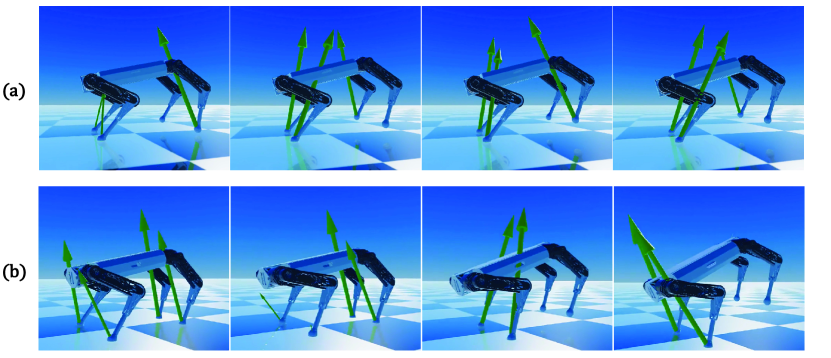
Figure 6: Snapshots of the front-leg rearing motion: (a) without and (b) with drift compensation. These depict the solution trajectory with the green arrow showing the contact impulse. In (a), the contact-implicit MPC employs force at a distance, violating the Signorini condition in positional space.

The adoption of a relatively large discretization time step ($dt=25$ ms) often leads to the occurrence of penetration or ‘force in the distance’ phenomenon. This behavior stems from satisfying the Signorini condition in velocity space, which ensures $v^{n}_{k,i+1}=0$, rather than $\phi_{k,i+1}=0$ in cases of contact. To address this issue, the drift term at the position level (Tassa et al., 2012; Carius et al., 2019), $\frac{\phi_{k,i}}{dt}$, is employed. This term ensures that the approximation of the next time step’s foot height approaches a zero value ($v^{n}_{k,i+1}+\frac{\phi_{k,i}}{dt}=0$), as derived in (25). By integrating the drift term, violations of the Signorini condition in positional space (e.g., force exerted at a distance) are mitigated, as demonstrated in Figure 6.

While the drift compensation for contact-implicit trajectory optimization is already introduced in (Carius et al., 2019), our study further includes its effect in the gradient. By analytically computing the gradient of contact impulse, we seamlessly incorporate the gradient of the drift component (which reduces to the contact Jacobian).

5.3 Gradient for Backward Pass

In the DDP backward pass, we initially compute the analytic gradient of the contact impulse based on the relaxed complementarity constraint. The computed gradients of contact impulse are used in obtaining the gradient $\mathbf{f}_{\mathbf{x}}$ and $\mathbf{f}_{\mathbf{u}}$ through the gradient of $\mathbf{q}_{i+1}$ and $\mathbf{\dot{q}}_{i+1}$, which are computed from the gradient of $\ddot{\mathbf{q}}_{i}$ through the semi-implicit Euler integration equation.

The equation of forward dynamics is written as,

$$\ddot{\mathbf{q}}_{i}=\mathbf{M}_{i}^{-1}(-\mathbf{h}_{i}+\mathbf{B}\mathbf{u}_{i}+\mathbf{J}_{i}^{T}\bm{\lambda}_{i}/dt),$$

and the derivative of the forward dynamics is written as,

$$\frac{\partial\ddot{\mathbf{q}}_{i}}{\partial\mathbf{q}}= \frac{\partial\mathbf{M}_{i}^{-1}}{\partial\mathbf{q}}(-\mathbf{h}_{i}+\mathbf{B}\mathbf{u}_{i}+\mathbf{J}_{i}^{T}\bm{\lambda}_{i}/dt)-\mathbf{M}_{i}^{-1}\frac{\partial\mathbf{h}_{i}}{\partial\mathbf{q}}$$ (26)

$$+\mathbf{M}_{i}^{-1}\frac{\partial\mathbf{J}_{i}^{T}}{\partial\mathbf{q}}\bm{\lambda}_{i}/dt+\mathbf{M}_{i}^{-1}\mathbf{J}_{i}^{T}\frac{\partial\bm{\lambda}_{i}}{\partial\mathbf{q}}/dt,$$

$$\frac{\partial\ddot{\mathbf{q}}_{i}}{\partial\dot{\mathbf{q}}}= -\mathbf{M}_{i}^{-1}\frac{\partial\mathbf{h}_{i}}{\partial\dot{\mathbf{q}}}+\mathbf{M}_{i}^{-1}\mathbf{J}_{i}^{T}\frac{\partial\bm{\lambda}_{i}}{\partial\dot{\mathbf{q}}}/dt,$$

$$\frac{\partial\ddot{\mathbf{q}}_{i}}{\partial\mathbf{u}}= \mathbf{M}_{i}^{-1}\mathbf{B}+\mathbf{M}_{i}^{-1}\mathbf{J}_{i}^{T}\frac{\partial\bm{\lambda}_{i}}{\partial\mathbf{u}}/dt.$$

For efficient computation, we first calculate the analytical derivative of the articulated body algorithm (ABA) (Carpentier and Mansard, 2018; Carpentier et al., 2019), excluding the derivatives of the contact Jacobian, $\mathbf{M}_{i}^{-1}\frac{\partial\mathbf{J}_{i}^{T}}{\partial\mathbf{q}}\bm{\lambda}_{i}/dt$, and the contact impulse component. The frame of the Jacobian should align with the frame of the contact impulse. Therefore, to compute the term $\mathbf{M}_{i}^{-1}\frac{\partial\mathbf{J}_{i}^{T}}{\partial\mathbf{q}}\bm{\lambda}_{i}/dt$, we utilize the kinematic hessian, $\frac{\partial\mathbf{J}_{i}}{\partial\mathbf{q}}$, in the contact frame. Finally, we incorporate the computed gradient of the contact impulse into the equation (26). Notably, the entire gradient computation takes around $70~{}\mu s$ under the most demanding scenario with all four contact points in clamping cases, tested on a desktop PC with an AMD Ryzen 5 3600X processor.

6 Implementation Detail for Motion Execution

This section examines the specifics of implementing real-world experiments. While the contact-implicit DDP (CI-DDP) framework is promising for motion generation, its initialization is sensitive to discrepancies in the initial state, presenting a challenge in robot control.

The optimization process is initialized by utilizing the state-control trajectory $\mathbf{x}_{0},\ldots,\mathbf{x}_{N-1},$ $\mathbf{u}_{0},\ldots,\mathbf{u}_{N-2}$, which is shifted by one time step from the solution of the previous MPC problem. This initialization provides an effective starting point for subsequent optimization problem (Diehl et al., 2002). It enhances convergence and guides the optimization towards the intended local minimum, ensuring motion continuity. However, the actual initial state, represented by $\mathbf{\tilde{x}}_{0}$ (the current estimated state), often deviates from $\mathbf{x}_{0}$, the state anticipated in the previous MPC problem. This discrepancy leads to complications within contact-implicit approach. In single shooting schemes, initialization is performed by successively integrating the control input trajectory, $\mathbf{u}_{0},\ldots,\mathbf{u}_{N-1}$, starting from the deviated initial state, $\mathbf{\tilde{x}}_{0}$, rather than $\mathbf{x}_{0}$. Given the hybrid model inherent in the contact-implicit method, even slight discrepancies can prompt a cascade of contact mode changes throughout the prediction horizon (Posa et al., 2014). This frequently results in trajectory divergence, leading to motion failures.

To address the aforementioned challenges, the FDDP algorithm (Mastalli et al., 2020, 2022a), a multiple-shooting variant of DDP, is employed, as multiple shooting (Bock and Plitt, 1984) could reduce the high sensitivity issue of single shooting (Wensing et al., 2023). FDDP accepts state-control trajectories for initialization, where the initialized state trajectory, $\mathbf{x}_{0},\ldots,\mathbf{x}_{N}$, implicitly guides contact modes consistent with the previous solution. Therefore, the initial state discrepancy ($\mathbf{\tilde{x}}_{0}\neq\mathbf{x}_{0}$) does not lead to divergence of trajectory due to unwanted contact mode variations such as in single shooting scheme. Although the dynamics gap exists due to initial state discrepancy, the FDDP algorithm progressively reduces these gap in the early stage of optimization.

In the following subsections, we detail this issue by contrasting the single shooting and multiple shooting schemes in the contact-implicit MPC framework. Additionally, an overview of the feedback control is provided.

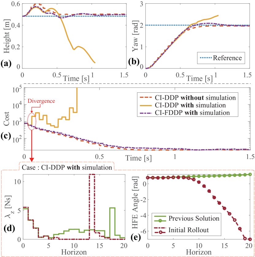
Figure 7: Comparison of Contact-implicit MPC performance under the three cases: 1) CI-DDP without simulation. 2) CI-DDP with simulation. 3) CI-FDDP with simulation. (a) and (b) represent the resulting height and yaw, respectively, while (c) indicate the cost associated with each sequential MPC problem. Within the “CI-DDP with simulation” scenario, the initial divergence is marked with red dots in (c). For this instance, the deviations of the state trajectory from the previous MPC solution and the current initial roll-out trajectory are depicted in (d)-(e): (d) RF leg’s normal contact impulse, and (e) RF leg’s HFE angle.

6.1 Single Shooting in Contact-implicit MPC

The results in Figure 7 demonstrate the initialization issue of the single shooting scheme stemming from initial state discrepancies. The contact-implicit MPC performance is analyzed under the three cases: 1) CI-DDP without simulation. In this scenario, the initial state, $\mathbf{\tilde{x}}_{0}$, is directly taken as $\mathbf{x}_{0}$. This ensures that there is no initial state discrepancy, in line with solving a trajectory optimization problem in a receding horizon fashion. 2) CI-DDP with simulation. 3) Contact-implicit FDDP (CI-FDDP) with simulation. For 2) and 3) cases, RaiSim simulator (Hwangbo et al., 2018) with 1 ms integration time step is used, and the MPC runs at 40 Hz. In these cases, the initial state discrepancies are inevitable, primarily due to the first-order discretization with a relatively large time step of $dt=25$ ms (Manchester et al., 2019). The reference body yaw angle is set as 2.0 rad, inducing a turning motion.

In the case of “CI-DDP without simulation”, the contact-implicit MPC using a single shooting method generates multi-contact motion, achieving the desired configuration, as depicted in Figure 7 (a)-(c). However, the case of “CI-DDP with simulation” exhibits divergence in the early stages of the overall motion, as shown in Figure 7.

In CI-DDP cases, initialization is achieved by a roll-out of the torque trajectory from the previous solution. However, within the hard contact model, where forces acting at a distance do not exist, a slight height difference of foot can lead to unplanned contact loss. In Figure 7 (d), the right front (RF) leg is shown to lose ground contact prematurely. Instead of maintaining contact throughout the entire prediction horizon (N=20), the foot loses contact after just 5 time steps. Consequently, this alters the torque deployment, originally planned for ground reaction force (GRF), accelerating the joint velocity and eventually resulting in the divergence of joint position, observed in Figure 7 (e). Such changes also pose challenges in maintaining balance due to insufficient GRF. As a result, the initialized trajectory deviates significantly from the solution trajectory of the previous step.

6.2 Multiple Shooting for Contact-implicit MPC

As evident in “CI-FDDP with simulation” of the yaw turning task depicted in Figure 7 (a)-(b), the CI-FDDP accomplishes the task despite initial state discrepancies. A comprehensive breakdown of this process is presented in Figure 8. At the start of motion, the first MPC problem is initialized with a feasible state-control trajectory, outlined in following subsection. Then, the dynamics gap is exclusively attributed to the initial state discrepancy, and that dynamics gap at the 0 th iteration can be expressed as follows:

$$\mathbf{\bar{f}}_{0}:=\mathbf{\tilde{x}}_{0}\ominus\mathbf{x}_{0}\neq\mathbf{0},$$

$$\mathbf{\bar{f}}_{i+1}:=\mathbf{f}(\mathbf{x}_{i},\mathbf{u}_{i})\ominus\mathbf{x}_{i+1}=\mathbf{0},\quad{\scriptstyle\forall i=\{0,1,...,N-1\}}.$$

During the line search procedure in the forward pass, the initial roll-out state $\mathbf{\hat{x}}_{0}$ is determined along the step size $\alpha$ as follows: $\mathbf{\hat{x}}_{0}:=\mathbf{\tilde{x}}_{0}\oplus(\alpha-1)\mathbf{\bar{f}}_{0}$, where it denotes the interpolation point lying between $\mathbf{\tilde{x}}_{0}$ and $\mathbf{x}_{0}$. If the roll-out trajectory is approved according to the acceptance condition, then the roll-out state $\mathbf{\hat{x}}_{i}$ is adopted as shooting state $\mathbf{x}_{i}$, and this entire process iterates until the gap is reduced to zero. This gap reduction is illustrated in Figure 8 (a). Furthermore, the shooting state trajectory is updated along the iterations, observed in Figure 8 (b). In each iteration, the optimizer incrementally adjusts the trajectory by pulling the 0 th shooting state $\mathbf{x}_{0}$ closer to the initial state $\mathbf{\tilde{x}}_{0}$, facilitated by the progressive modification using step size $\alpha$. Meanwhile, the other states are closely preserved to the state of the previous iteration, due to the feedback term that involves the gain K in equation (5). Therefore, the contact modes are also implicitly guided to align with prior modes.

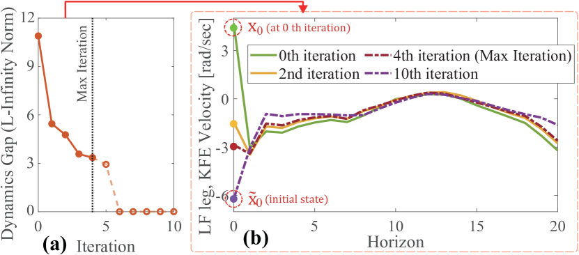
Figure 8: The detailed description for the case of CI-FDDP for the yaw turning task, shown in Figure 7. (a) illustrates the gap reduction process across iterations, specifically for the instance with the largest gap in this case. Here, the max iteration is set as 4. (b) denotes the LF leg KFE velocity trajectory along the horizon at each iteration.

In conclusion, during the initialization process, CI-FDDP prioritizes consistency with prior contact modes by trading off feasibility, thereby enhancing the robustness of initialization. Conversely, CI-DDP risks deviating from prior contact modes and often diverges as a result, when integrating the state trajectory to achieve feasible initialization. In practice, CI-FDDP also manages unexpected slippage (Section 7.2.5), and conducts real-robot experiments despite model imperfections and state estimation uncertainties.

6.2.1 Initial Feasible Trajectory.

Prior to the initial MPC problem, we solve a trajectory optimization problem under the reference configuration with a standing posture, using the same framework. This aims to determine a feasible state-control trajectory that maintains the robot in a standing motion. All varied motions in this paper stem from this standing motion initialization and, therefore, do not require the task-specified pre-planned contact modes or trajectories.

6.2.2 Maximum Iteration.

To ensure real-time computation requirements, we limit the maximum number of iterations of the CI-FDDP as 4, aligning with real-time constraints. The optimizer requires minimal iterations to reduce the dynamics gap, as observed in Figure 8 (a), and explore contact modes in each iteration.

6.3 Feedback Control

Within the discretization time step of 25 ms, using open-loop feed-forward force from contact-implicit MPC can lead to reduced control performance. Specifically, missed contact might result in large swing leg divergence in a contact-implicit setting. Consequently, in many contact-implicit approaches (Neunert et al., 2017, 2018; Carius et al., 2018, 2019; Aydinoglu et al., 2023), a PD control is utilized to address this issue. Similar to Youm et al. (2023), we proposed and incorporated a PD control that combines feed-forward torques with feedback actions, given by,

$$\mathbf{p}_{\text{target}}=\mathbf{u}^{*}_{0}/K_{p}+\mathbf{p}_{\text{des}},$$

$$\mathbf{u}_{\text{cmd}}=\mathbf{K}_{p}(\mathbf{p}_{\text{target}}-\mathbf{p})+\mathbf{K}_{d}(\dot{\mathbf{p}}_{\text{des}}-\dot{\mathbf{p}}).$$

Here, $\mathbf{p}_{\text{des}}$ and $\dot{\mathbf{p}}_{\text{des}}$ are chosen based on the next time step’s joint state from the solution trajectory of the CI-FDDP. If the current joint position and velocity, $\mathbf{p}$ and $\dot{\mathbf{p}}$, are close to $\mathbf{p}_{\text{des}}$ and $\dot{\mathbf{p}}_{\text{des}}$, respectively, $\mathbf{u}_{\text{cmd}}$ aligns with the feed-forward torque $\mathbf{u}^{*}_{0}$. Feedback actions increase as they deviate from $\mathbf{p}_{\text{des}}$ and $\dot{\mathbf{p}}_{\text{des}}$.

7 Results

In this section, we present the results of our framework for quadruped robots through simulation and experimental trials. First, we analyze the effect of the relaxation variable $\rho$ using a 2D planar quadruped model. Next, we showcase multi-contact motions for various desired configurations in 3D simulations, and compare our framework with MuJoCo MPC (Howell et al., 2022). Lastly, we validate the contact-implicit MPC framework with hardware experiments, illustrating trot and front-leg rearing motions.

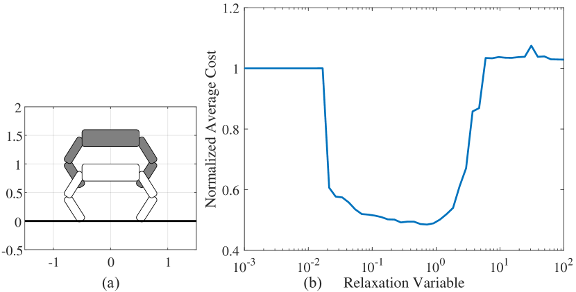
Figure 9: Relation between relaxation variable and average cost for jumping up task : (a) 2D environment, grey robot for the reference trajectory and white robot for the present robot configuration. (b) Result of the average cost for 5 sec motion according to the relaxation variable.

7.1 Effect of the Relaxation Variable

In this subsection, we investigate the impact of the relaxation variable $\rho$. The introduction of the relaxation variable allows the gradient to navigate motions that break contact, thanks to the smooth curve in the relaxed complementarity constraint. To evaluate this, we conducted a 2D simulation with a planar quadruped robot, consistent with the settings from our earlier publication (Kim et al., 2022). The contact-implicit MPC solely employed a regulating cost with a fixed reference configuration. Figure 9 (a) illustrates the 2D setup and Figure 9 (b) maps the average cost against the relaxation variable.

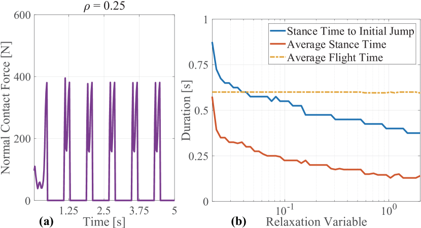
Figure 10: Periodic jumping motion analysis: (a) Contact impulse for 0.25 relaxation variable, indicating periodic jumps. (b) Average stance time versus relaxation variable.

In this scenario, a reference trajectory is set significantly above the robot. Therefore, a periodic jumping motion, where the robot continuously strives to approach the reference configuration, would result in a lower cost compared to a stationary standing motion. Without relaxation, the resulting motion remains standing still, aligning with the initial trajectory where all feet are in contact. This trend continues until the relaxation variable exceeds 0.02. Beyond this value, the robot exhibits a periodic jumping motion, achieving a lower cost than standing motion. However, when the relaxation variable is excessively increased, exceeding 6 in this example, the robot prematurely attempts to jump without accumulating sufficient contact impulse. This premature trial leads to in-place bouncing, increasing the cost due to unnecessary movement, as illustrated in Figure 9 (b). All the discovered motions are shown in Extension 3. A key observation is that there are no modifications to the cost function, such as weight adjustments or the inclusion of time-dependent costs. The introduction of the smooth gradient (through relaxation) alone enables the emergence of the jumping motion, indicating the convergence to a lower-cost solution within the same optimal control problem.

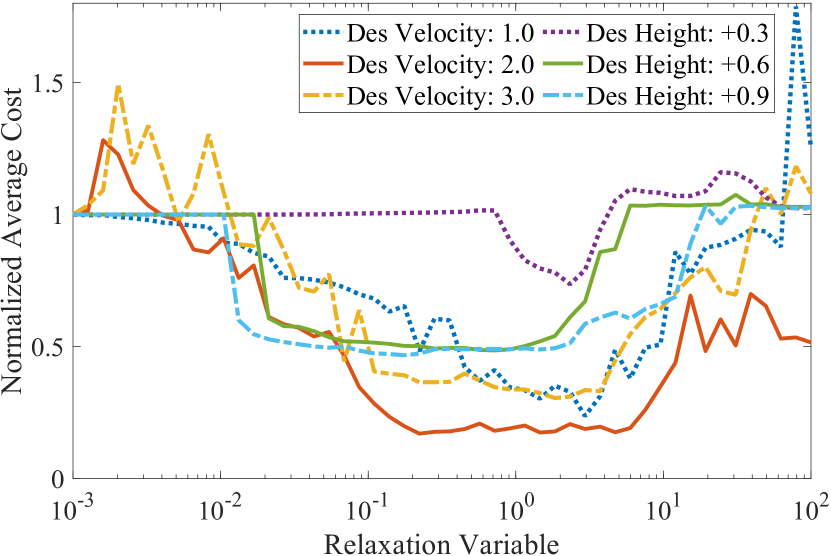
Figure 11: Result of the cost according to the relaxation variable for jumping up task 0.3  m, 0.6  m, and 0.9  m, and moving forward task 1.0  m/s, 2.0  m/s, and 3.0  m/s.

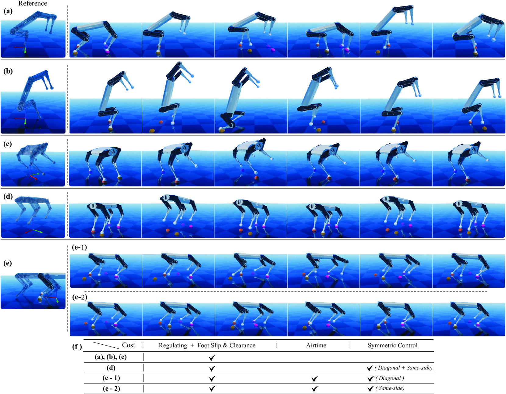
Figure 12: 3D simulation outcomes for various reference configurations are presented using the proposed contact-implicit MPC approach. The transparent robot on the left side is denoted to the reference configuration, while the robot snapshot depicts the resulting simulation with colored spheres indicating planned next contact points. (a) Target pitch: 0.6 rad (with height offset 0.1 m). (b) Target pitch: 1.2 rad (with height offset 0.1 m). (c) Target roll: 0.6 rad (with height offset 0.1 m). (d) Target height: nominal height + 0.25 m. (e) Target position along the x-axis: current robot x position + 0.55 m. (f) A table detailing cost types for each motion.

We further investigate the effect of relaxation variable $\rho$ within the scope of [0.02, 2], exhibiting periodic jumping motions. Figure 10 (a) depicts the contact forces associated with this periodic motion, and Figure 10 (b) presents the average stance time with the time taken for the initial jump. Notably, there is a consistent decrease in average stance time as $\rho$ increases (Figure 10 (b)). This implies that the relaxation variable guides the optimizer to initiate contact-breaking motions. Consequently, the optimizer generates multi-contact motions that potentially reduce the cost as seen in Figure 9 (b).

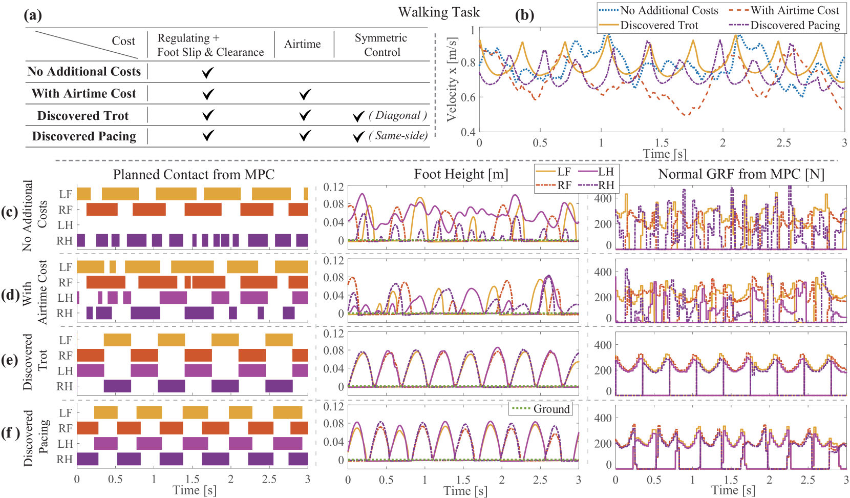
Figure 13: Analysis for the walking motions under different cost configurations: (a) Table showing cost components for each case. (b) Velocity profiles for each walking motion. (c)-(f) Display planned contact, swing leg trajectory on the z-axis, and the normal ground reaction force from MPC for each case.

Achieving a lower cost utilizing a smooth gradient is evident across various tasks. Figure 11 presents the average cost according to the relaxation variable for both ‘jumping up’ and ‘moving forward’ tasks. In the jumping-up task, reference trajectories are placed 0.3 m, 0.6 m, and 0.9 m higher than the robot’s starting position and are held constant. For the moving forward task, reference trajectories correspond to a steady forward movement with specified velocities of 1.0 m/s, 2.0 m/s, and 3.0 m/s. As shown in Figure 11, across different tasks, a consistent region around [0.1, 10] emerges where the cost is reduced below that of the no-relaxation case. This suggests that the effect of the smooth gradient is not task-dependent.

Therefore, the smooth gradient can facilitate the emergence of diverse motions as shown in Extension 8, including forward movement, continuous flipping, and sliding, all of which are achieved with a simple reference trajectory in 2D environment.

7.2 3D Simulation Results

7.2.1 Implementation of 3D Environment.

In 3D simulations, the HOUND quadruped robot was employed (Shin et al., 2022). Throughout all simulations, we fixed the relaxation variable $\rho$ at a value of $2.0$ for HOUND without additional adjustments. The entire 3D simulation process was facilitated by the RaiSim simulator (Hwangbo et al., 2018), with a 1 ms integration time step, devoid of control delays. For each MPC instance, the exact simulated state was taken as the initial state.

7.2.2 Various Quadruped Motions.

To validate the capacity of our contact-implicit MPC in generating diverse multi-contact motions, we display the results in Figure 12 and Extension 4, 5, and 6. As seen on the left side of Figure 12, the reference trajectory is formed by modifying only the body references (position and orientation in $\mathrm{SE}(3)$).

All motions are derived primarily using the regulating cost and foot slip and clearance cost. As illustrated in Figure 12 (a) and (b), front-leg rearing motions emerge from a desired pitch reference. The quadruped tries to balance on its front leg by adjusting foothold positions or swiftly kicking its hind leg to leap upwards, aiming to match the desired configuration. It is noticeable that the desired configuration involves only body rotation and does not specifically guide the CoM positioning beneath the support line between the front legs. Even when the desired posture is intrinsically unstable and not the system’s equilibrium, our proposed method repeatedly tries to align with the desired posture (Extension 4). This feature is also emphasized in the random rotation task (Figure 14, and Extension 6), where a target rotation is changed, showcasing seamless transitions between diverse references. Likewise, a side-leg rearing motion occurs with the desired roll angle reference, as depicted in Figure 12 (c).

Given a reference configuration positioned higher than the robot, our framework is capable of inducing a four-leg jumping motion, with an added symmetric control cost as depicted in Figure 12 (d). When the reference is updated to be in front of the robot’s current location, it results in a walking motion, as seen in Figure 12 (e). The methodology for producing this walking motion is elaborated in the following subsection. An important observation is that without the introduction of the smooth gradient (no-relaxation scenario), diverse multi-contact motions do not manifest under the same conditions. Instead, the resulting motions converge to a tilted posture with all feet in contact (see Extension 4).

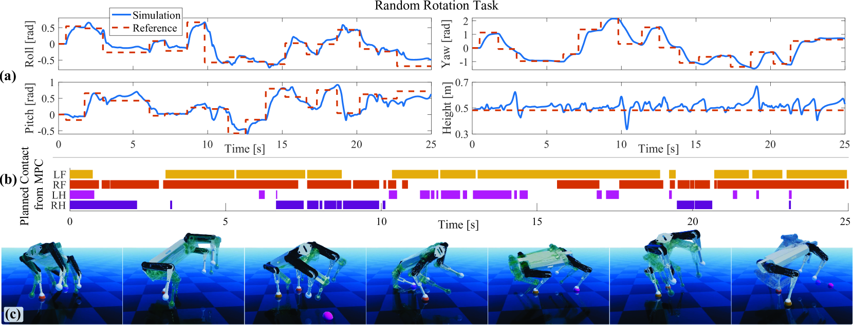
Figure 14: Analysis for the random rotation task, when the robot aligns with the reference configuration, the reference is subsequently changed: (a) Desired and resulting rotation angle (roll, pitch, yaw) and height. (b) MPC-planned contact. (c) Snapshots, where the green transparent robot indicates the alignment condition being satisfied.

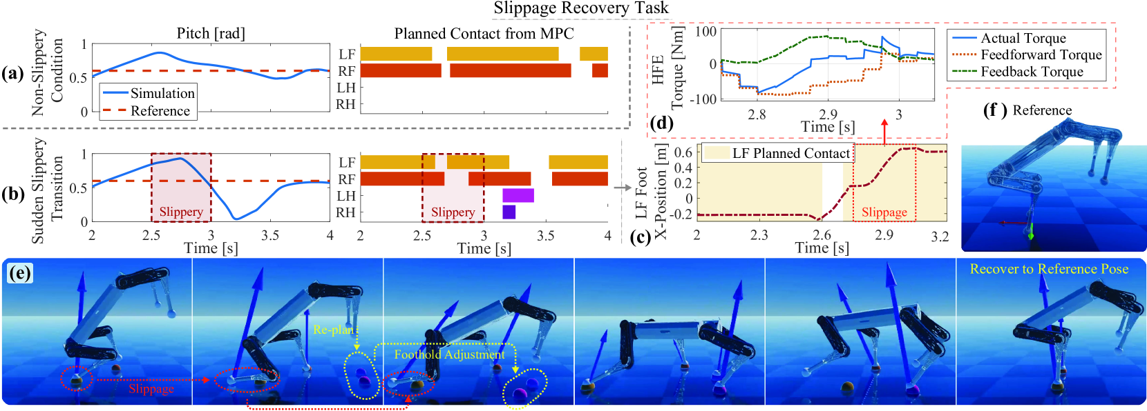
Figure 15: Analysis of the slippage recovery task, which involves an unexpected transition to slippery terrain, resulting in slippage: (a) Without transition to slippery terrain, (b) With transition to slippery terrain. Both scenarios (a) and (b) illustrate the reference and actual pitch angles, along with MPC-planned contacts. Subfigures (c)-(e) detail an instance of slippage involving the left front (LF) leg and the subsequent recovery behavior: (c) LF foot x-axis position, (d) LF leg’s HFE torque profiles including feedforward and feedback components, (e) Snapshots demonstrating re-planning and foothold adjustments after the slippage, with colored spheres indicating the planned next contact points. (f) Reference configuration.

7.2.3 Discovery of Gait.

Discovering natural gait motions in quadrupeds from scratch, without predefined contact sequences, is challenging due to the numerous possible contact combinations. Prior research (Neunert et al., 2017) struggled with adjusting the regulating cost to balance between running and final costs, as well as positions and velocities, to achieve natural gait patterns. To avoid this cost tuning, integrating a periodic cost encoding preferred gait (e.g., bending knee periodically) offers a feasible alternative (Neunert et al., 2018; Carius et al., 2019; Kim et al., 2022). In this work, we show that our framework identifies a walking motion without the aforementioned gait-encoded costs. Instead, we utilize four types of costs: regulating (equation (21)), foot slip and clearance (equation (22)), air time (equation (23)), and symmetric control (equation (24)). The outcomes are illustrated in Figure 13 and Extension 5. At each MPC problem, the reference configuration is set to be 0.55 m ahead of the current robot configuration to pull the robot in a forward direction.

Utilizing only basic costs (regulating, foot slip and clearance), a three-leg walking motion emerges, as shown in Figure 13 (c). The robot does not utilize the left hind (LH) leg and relies on the right hind (RH) leg, leading to chattering in the RH foot due to insufficient swing time. Introducing an air time cost yielded a four-legged motion, as in Figure 13 (d), engaging the LH leg and reducing the load on the RH leg. However, the motion remains non-cyclic, with a bias towards the front legs bearing most of the GRF (Figure 13 (d)) and a significant velocity deviation (Figure 13 (b)).

Incorporating a symmetric control cost, our framework discerns gait motions for trotting and pacing, as shown in Figure 13 (e) and (f), respectively. Despite all the costs not being periodically activated and the short 0.5-sec horizon, the resultant gait is cyclic and remains consistent across sequential MPC problems. The smooth gradient directs optimization towards the breaking contact of the foot to move forward, while the foot slip and clearance cost ensures proper foot lifting and prevents sliding. The air time cost encourages contact for feet that swing excessively long, and the symmetric control cost ensures that these movements are coordinated within the pair. By initializing each MPC problem with prior solutions, the entire motion style remains consistent. Additionally, the optimizer naturally selects distinct frequencies for trotting and pacing gaits. Also, the load required to support the body is evenly distributed through the front and hind legs, and the smooth swing leg trajectory is observed, as depicted in (e) and (f).

7.2.4 Random Rotational Task.

In this subsection, we explore the random rotation task. The target rotation is randomly set and adjusted upon meeting the success criteria. This task showcases our framework’s ability to handle various contact combinations in response to quickly changing reference configurations. The reference body rotation is uniformly sampled as roll, pitch $\sim U(-0.8,0.8)$ rad, and yaw difference $\sim U(-2,2)$ rad, with the yaw angle updated accordingly. The success criteria for the reference body rotation, $\mathbf{R}_{\text{ref}}$, is met when the angle of the rotation difference is under $10\,~{}\text{deg}$, $\|\epsilon_{\mathbf{R}}\|<0.174\,~{}\text{rad}$ (with $\epsilon_{\mathbf{R}}$ computed as $\text{log}(\mathbf{R}_{\text{ref}}^{T}\mathbf{R}_{\text{current}})^{\vee}$), and the body’s lateral deviation is below 0.4 m. The motion trajectory and reference body rotation are depicted in Figure 14 (a), while the identified contact sequences are displayed in Figure 14 (b). Figure 14 (c) displays the motion snapshots. Dynamic motions emerge, such as single and double-leg balancing and turning, rearing maneuvers, pivoting turns around a leg, and swift kick-back, which are available in Extension 6.

7.2.5 Slippage Recovery Task.

The re-planning capabilities of the proposed framework are demonstrated in the slippage recovery task. In this scenario, unexpected slippage is induced by a sudden, unknown change in the ground’s friction coefficient (from 0.8 to 0.25 and back to 0.8). Nevertheless, the robot swiftly recovers through the feedback policy and by re-planning in subsequent MPC problems. We present the recovery motions across various reference configurations in Extension 9, using the same settings in Figure 12.

For clarity, Figure 15 illustrates the slippage recovery process with a reference pitch angle of 0.6 rad. Under non-slippery conditions, a front-leg rearing motion emerges, as shown in Figure 15 (a). However, with a sudden, unknown friction drop (from 2.5 sec to 3.0 sec), slippage of the left front (LF) foot occurs (Figure 15 (c)), causing the robot to fail to balance on only the front two feet (Figure 15 (b)). Initially, the PD control addresses the LF leg’s positional deviation, by exerting torque in the opposite direction of the slippage (Figure 15 (d)). Subsequent MPC problems aim to stabilize the body by adjusting the other legs, notably re-planning to engage two hind legs and shifting the planned foot hold positions (Figure 15 (e)). In particular, following the slippage, the hind legs support the falling body, and the robot executes a backward kick to return to the reference pose (Figure 15 (e) and Extension 9). Despite unexpected disturbances, the framework swiftly adapts, recovers, and continues with the task’s progression.

7.2.6 Comparison with MuJoCo MPC.

We benchmark our framework against MuJoCo MPC (Howell et al., 2022; Tassa et al., 2014), a contact-implicit MPC framework, integrated with the MuJoCo simulator (Todorov et al., 2012). For the comparison, the iterative linear quadratic gaussian (iLQG) method in the MuJoCo MPC library is used, leveraging MuJoCo’s finite-difference gradient computation. Both frameworks tackle the identical optimal control problem. Specifically, a regulating cost is utilized with identical weights setting: generalized coordinate (pos xy, pos z, rotation, joint pos) set as (1, 10, 10, 0.1), generalized velocity (joint vel) at 5e-4, and control input at 5e-4. Both methods adopt a discretization time step of 20 ms for a 20-step horizon, totally to 0.4 seconds. The Unitree A1 quadruped robot is employed under the same control input constraints.

Our framework is tested on the Raisim simulator, while MuJoCo MPC employs the MuJoCo simulator, executing computations under the same desktop PC equipped with an AMD Ryzen 5 3600X processor. The reference configurations specify desired pitch angles from 0.2 rad to 1.0 rad, with a height goal of 0.28 m. Figure 16 presents a comparison of tracking errors across all scenarios.

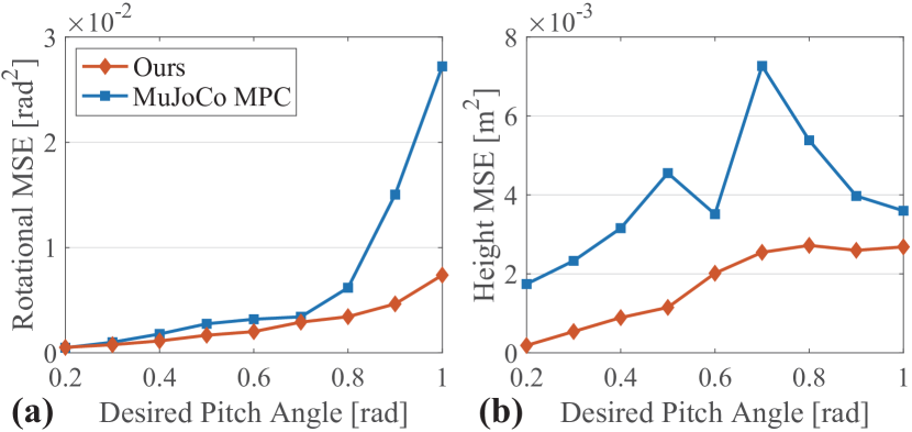
Figure 16: Comparing our proposed framework with the iLQG of the MuJoCo MPC for a desired pitch task ranging from 0.2 rad to 1.0 rad, where each task spans 10 seconds: (a) Mean squared error (MSE) for rotational angle error. (b) MSE for height error.

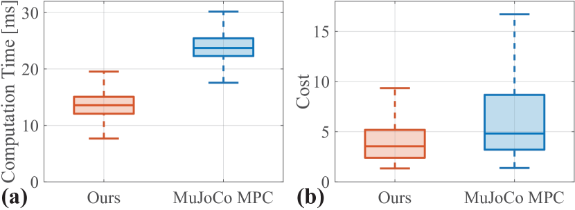
Figure 17: Box plot comparison of (a) computation times and (b) costs for all tasks in Figure 16. Each task comprises 500 MPC problems, corresponding to a 10-second duration.

In our approach, the relaxation variable $\rho$ is set as 1.0. This explicit relaxation in the analytical gradient promotes repeated attempts at a rearing motion, thereby efficiently aligning the robot with both the desired pitch angle and height. This results in minimal angle error, with only slight compromises in height tracking for steeper pitch angles (0.7 rad to 1.0 rad). For the MuJoCo MPC approach, they employ finite differences combined with soft contact simulation (Todorov, 2011, 2014). Therefore, the smoothness of the gradient is determined by the soft contact model. This implies that the range of smoothness could be limited due to the trade-off between smoothness and contact feasibility. The restricted smoothness can induce minimal contact breakage motions, such as body tilting with all foot contacts or handstanding with body touch (Extension 7). This can compromise height tracking (Figure 16 (b) for 0.5-0.8 rad desired pitch), and angle tracking (Figure 16 (a) for desired pitches over 0.8 rad). Therefore, our method generally results in a lower cost, as reflected in the overall cost distribution in Figure 17 (b). Simulation results are available in Extension 7.

The average computation time for each optimal control problem is shown in Figure 17 (a). Given the real-time constraint (sampling time 20 ms), the maximum iteration for the problem is determined. Due to this constraint, the iLQG of the MuJoCo MPC operates in a single iteration, while our method allows up to four iterations. These iterations in our approach aim to reduce the feasibility gap and explore alternative contact modes. Notably, even with the increased number of iterations, we achieve a shorter computation time, as depicted in Figure 17 (a). This is attributed to our efficient analytical gradient computation.

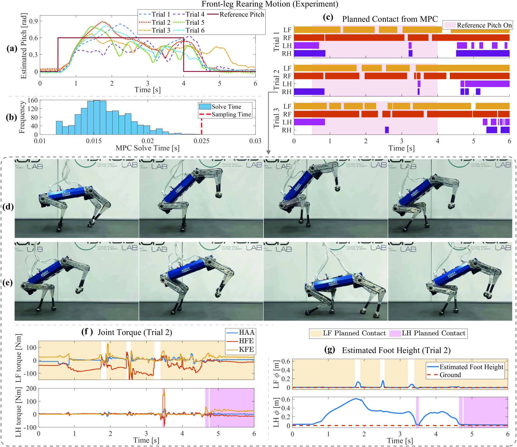
Figure 18: Experimental results of the front-leg rearing motion for 6 trials: (a) Estimated pitch angle with a target of 0.6 rad over 3.5 sec. (b) Histogram of MPC computation times. (c) MPC-derived contact sequences for Trials 1-3. (d-e) Motion snapshots, (f) Joint torques, and (g) Estimated foot heights for Trial 2.

7.3 Experiments

Finally, we conducted experiments to validate the proposed framework in two scenarios: 1) Executing a front-leg rearing motion with a fixed pitch reference configuration and 2) Performing trot motion directed by a joystick command.

7.3.1 Experimental Setup.

The HOUND quadruped robot weighing 45 kg (Shin et al., 2022) was employed for the experiments. The maximum joint torques are 200 Nm for the hip abduction/adduction (HAA) and hip flexion/extension (HFE) joints and 396.7 Nm for the knee flexion/extension (KFE) joint. The maximum joint velocities are 19.2 rad/s for HAA and HFE joints and 9.7 rad/s for the KFE joint at 73 Volts (based on experimental findings). A single onboard computer with an Intel(R) Core(TM) i7-11700T CPU @ up to 4.6 GHz is utilized for solving the contact-implicit MPC problem, EtherCAT communication, PD control, and state estimation. The MPC problems are solved using Box-FDDP (Mastalli et al., 2022a), consistent with the simulation environment, incorporating feedback PD control. The MPC problem operates at a frequency of 40 Hz. The joint position and velocity are sampled at 2 kHz, leading the PD control to function at the same 2 kHz frequency, while the state estimator works at 1 kHz.

7.3.2 State Estimation.

For body state estimation, we employ a linear Kalman filter algorithm that fuses leg kinematics and IMU information. This algorithm is used to estimate the body’s linear position and velocity with respect to the global (world) frame. Additionally, we utilize a generalized momentum method (De Luca et al., 2006) to estimate the foot contact state. This detected contact state informs the Kalman filter.

To address the delay caused by the computation time of the MPC, we employ state prediction approach similar to Mastalli et al. (2022b). We utilize the predicted generalized coordinate, $\mathbf{q}_{\delta}$, for the initial state $\mathbf{\tilde{x}}_{0}$ of the MPC problem. The prediction step is expressed as:

$$\mathbf{q}_{\delta}=\mathbf{q}+\dot{\mathbf{q}}\delta t,$$

where $\mathbf{q}$ and $\dot{\mathbf{q}}$ represent the currently estimated generalized coordinate and generalized velocity, respectively. The time interval $\delta t$ is set to 18 ms, accounting for the average computation time and allowing for potential peak durations.

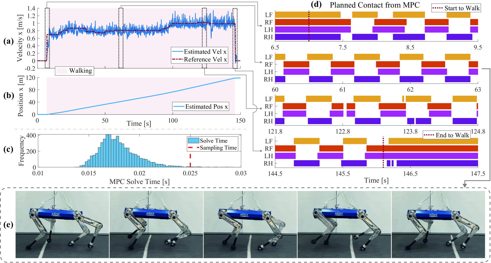
Figure 19: Experimental results of the walking motion for the discovered trot motion: (a) Estimated velocity with a target velocity in the x-direction. (b) Estimated x-position. (c) Histogram of MPC computation times. (d) MPC-derived contact sequences. (e) Motion snapshot.

7.3.3 Front-leg Rearing Motion.

The reference is set to a pitch angle of 0.6 rad for making rearing motion, with a 0.3 m positional x offset and 0.1 m height offset. This desired configuration is maintained for 3.5 seconds, and then returning to a nominal configuration with a 0 rad pitch angle. The relaxation variable is set as 2.0, and the regulation cost and the foot slip and clearance cost are used with weights consistent with the simulation setting(Figure 12). The result of a total of 6 trials is depicted in Figure 18 (a), and the capabilities of real-time computation is verified in Figure 18 (b). For the first three trials, the planned contact sequences are shown in Figure 18 (c). The torque trajectories and foot trajectories are shown in Figure 18 (f) and (g), respectively. All trials are available in Extension 1.

The main motion is driven by a regulating cost. The desired pitch angle induces a front-leg rearing motion while other components, such as nominal joint configuration, act to regulate excessive deviations of legs. The smooth gradient facilitates maneuvers of breaking contact, enabling initial kick-ups or foot adjustments for balancing.

All trials exhibit varied motions, even though they show a common motion trend, as observed in Figure 18 (a) and (c). This variation arises because the framework does not rely on a fixed trajectory, typically computed in offline trajectory optimization, but instead generates motions online in a real-time fashion. Consequently, it allows adaptive responses to each specific situation.

The rearing motion starts with a hind leg kick, and the robot aims to stabilize its body pitch near the target angle using front feet. If the body leans forward, the robot either pivots on one front leg or adjusts both front feet to gain reverse momentum from the ground reaction forces, as shown in Figure 18 (d). If leaning backward, the robot initially tries to balance using its front feet, and if the momentum continues downward, it resorts to a backward kick to elevate the body, depicted in Figure 18 (e). In cases where the initial kick is not sufficient, the robot will attempt another kickback (Trial 4). Despite balancing failures or missed contacts, the robot adjusts using other legs, as demonstrated in Trials 3 and 4. In contrast to more reactive controllers that rapidly adjust to maintain balance, our MPC exhibits a forward-planning motion style, such as waiting for the hind legs to make contact with the ground before executing a kick-back, ensuring consistency across subsequent MPC problems.

7.3.4 Trot Motion.

To assess the viability of the real-time discovery of gait in subsection 7.2.3, we tested for the trot motion. Consistent with the simulation settings, there is no periodic cost applied to enforce a specific gait. Forward and yaw velocity commands, $v_{\text{des}}$ and $\omega_{\text{des}}$ respectively, dictate the reference configuration. This is computed as $(v_{\text{des}}+0.1)dtN$ in front of the robot’s current pose, with a yaw deviation of $\omega_{\text{des}}dtN$. The results illustrate around 120 m treadmill walk along 140 seconds, as seen in Figure 19 (b). The velocity ranged between [0.7,1.0] m/s (Figure 19 (a)). This experiment allowed for online gait identification, revealing a trot as visualized in Figure 19 (d) and a snapshot in Figure 19 (e). MPC problem computation times are presented in Figure 19 (c). While no periodic cost was introduced to enforce a trot gait, the discovered gait showed minor deviations from a conventional trot at higher desired velocities, as observed in Figure 19 (d). Additionally, smooth gait transitions during the start and stop phases were also identified, as depicted in Figure 19 (d). The full video is available in Extension 2.

7.3.5 Limitation of Experiment.

While simulations allow for dynamic motion discovery, real-world experiments present difficulties due to the absence of an accurate state estimator. Our framework depends on roll-out trajectories for contact planning, being sensitive to the precision of initial state estimations. Although it can address certain discrepancies between expected and actual initial states (e.g., due to large discretization time step), the challenge here is that the framework plans based on an incorrectly estimated state. Specifically, body height estimation is crucial as it dictates potential contact modes by determining foot height through kinematics. Inaccurate height estimation can lead to misplanned contacts and eventual failures of motion. This becomes more critical in dynamic motions with fewer contacts, where balance relies solely on one or two feet. Hence, while our framework handles a range of dynamic motions, extreme motions in experiments, such as rearing motions with longer duration or steeper desired pitch angles, remain an area for future work.

8 Conclusion

In this work, we introduce a contact-implicit MPC framework that simultaneously generates and executes multi-contact motions without pre-planned contact mode sequences or trajectories. The hard contact model based on the complementarity constraint is utilized in the DDP-based algorithm, with the analytic gradient of contact impulse. To explore new contact modes, especially involving breaking contact, an analytically computed smooth gradient of contact impulse is proposed, based on the relaxed complementarity constraint. By leveraging the smooth gradient, the framework can discover diverse multi-contact motions, starting from fully-contacted standing poses. To enhance the tractability of the motions such as enough foot lifting, we have incorporated differentiable cost terms. Furthermore, for ensuring stable motion execution, the multiple shooting variant of DDP is employed. Our framework’s efficacy is demonstrated through various multi-contact motions using the 45 kg quadruped robot, HOUND, in both simulated environments and real-world experimental tests.

In this study, we mainly consider contacts between the feet of quadrupeds and ground to ease the computations. While a range of motions is identified with this consideration, a more generalized approach for future work would involve accounting for contacts between other body parts and various objects.

Lastly, while our proposed method demonstrates potential, its sensitivity to state estimation has posed challenges in realizing highly dynamic motions in real-world experiments. Future work could benefit from leveraging learning-based approaches to enhance robustness, such as employing learning-based estimation or integrating an auxiliary control term in place of the conventional PD control. Also, the diverse set of motions generated by our framework can serve as valuable prior motion data for learning-based controllers, as seen in works such as Peng et al. (2021, 2022); Wu et al. (2023).

The author(s) disclosed receipt of the following financial support for the research, authorship, and/or publication of this article: This research was financially supported by the Institute of Civil Military Technology Cooperation funded by the Defense Acquisition Program Administration and Ministry of Trade, Industry and Energy of Korean government under grant No. UM22207RD2.

Notes

1. 1 In contrast to previous method in Yu et al. (2018), which emphasizes global symmetry through mirroring actions of counterparts (e.g., right legs mirroring left legs), our cost focuses on within-pair symmetry (e.g., right legs together, left legs together).
2. 2 While the penetration phenomenon is less apparent with smaller time steps, such as 1 ms, reducing $dt$ in trajectory optimization is limited by the need to extend the prediction horizon for consistent prediction time.
3. 3 The contact frame aligns with the CENTERED frame in (Kleff et al., 2022). The CENTERED frame is centered to the local frame, yet its axes remain oriented consistently with the WORLD frame at all times.
4. 4 As illustrated in Equation 19, computing the gradient of the contact impulse $\frac{\partial\bm{\lambda}}{\partial\xi}$ requires terms in $\frac{\partial\ddot{\mathbf{q}}_{i}}{\partial\xi}$. For these terms, we reuse the computed analytical derivative of the ABA without additional computation.
5. 5 To ensure a safe initialization, we set the last control input $\mathbf{u}_{N-1}$ to zero, instead of directly copying $\mathbf{u}_{N-2}$ and subsequently simulate the last state $\mathbf{x}_{N}$. This mitigates potential issues, such as divergence in the last joint state resulting from the direct copy of incompatible large torque.
6. 6 The detected contact state is also used to mitigate body height drift (Bledt et al., 2018) by assuming that the height of supporting feet are zero.
7. 7 The motion is tried 3 times consecutively with short-term breaks (under 5 seconds), and the experiment is conducted twice.

Appendix A

Index to Multimedia Extension

Extension	Media Type	Description
1	Video	Real-world experimental results on a quadruped demonstrating front-leg rearing motion.
2	Video	Real-world experimental results on a quadruped showcasing real-time discovery of a trot gait.
3	Video	Resultant motion of varying the relaxation variable in a 2D environment.
4	Video	3D simulation results of various reference configurations.
5	Video	3D simulation results demonstrating gait discovery.
6	Video	3D simulation results for a random rotation task.
7	Video	3D simulation comparison between our method and MuJoCo MPC.
8	Video	Additional motion results in a 2D environment.
9	Video	3D simulation results of re-planning in response to slippage.

References

- Aydinoglu and Posa (2022) Aydinoglu A and Posa M (2022) Real-time multi-contact model predictive control via admm. In: 2022 International Conference on Robotics and Automation (ICRA). IEEE, pp. 3414–3421.
- Aydinoglu et al. (2023) Aydinoglu A, Wei A and Posa M (2023) Consensus complementarity control for multi-contact mpc. arXiv preprint arXiv:2304.11259 .
- Bledt and Kim (2019) Bledt G and Kim S (2019) Implementing regularized predictive control for simultaneous real-time footstep and ground reaction force optimization. In: 2019 IEEE/RSJ International Conference on Intelligent Robots and Systems (IROS). pp. 6316–6323. 10.1109/IROS40897.2019.8968031.
- Bledt et al. (2018) Bledt G, Powell MJ, Katz B, Di Carlo J, Wensing PM and Kim S (2018) Mit cheetah 3: Design and control of a robust, dynamic quadruped robot. In: 2018 IEEE/RSJ International Conference on Intelligent Robots and Systems (IROS). IEEE, pp. 2245–2252.
- Bock and Plitt (1984) Bock HG and Plitt KJ (1984) A multiple shooting algorithm for direct solution of optimal control problems. IFAC Proceedings Volumes 17(2): 1603–1608.
- Carius et al. (2018) Carius J, Ranftl R, Koltun V and Hutter M (2018) Trajectory optimization with implicit hard contacts. IEEE Robotics and Automation Letters 3(4): 3316–3323.
- Carius et al. (2019) Carius J, Ranftl R, Koltun V and Hutter M (2019) Trajectory optimization for legged robots with slipping motions. IEEE Robotics and Automation Letters 4(3): 3013–3020.
- Carpentier and Mansard (2018) Carpentier J and Mansard N (2018) Analytical derivatives of rigid body dynamics algorithms. In: Robotics: Science and systems (RSS 2018).
- Carpentier et al. (2019) Carpentier J, Saurel G, Buondonno G, Mirabel J, Lamiraux F, Stasse O and Mansard N (2019) The pinocchio c++ library : A fast and flexible implementation of rigid body dynamics algorithms and their analytical derivatives. In: 2019 IEEE/SICE International Symposium on System Integration (SII). pp. 614–619. 10.1109/SII.2019.8700380.
- Chatzinikolaidis and Li (2021) Chatzinikolaidis I and Li Z (2021) Trajectory optimization of contact-rich motions using implicit differential dynamic programming. IEEE Robotics and Automation Letters 6(2): 2626–2633.
- Chen et al. (2023) Chen H, Hong Z, Yang S, Wensing PM and Zhang W (2023) Quadruped capturability and push recovery via a switched-systems characterization of dynamic balance. IEEE Transactions on Robotics .
- Cleac’h et al. (2021) Cleac’h SL, Howell T, Schwager M and Manchester Z (2021) Fast contact-implicit model-predictive control. arXiv preprint arXiv:2107.05616 .
- Corbères et al. (2023) Corbères T, Mastalli C, Merkt W, Havoutis I, Fallon M, Mansard N, Flayols T, Vijayakumar S and Tonneau S (2023) Perceptive locomotion through whole-body mpc and optimal region selection. arXiv preprint arXiv:2305.08926 .
- Cottle et al. (2009) Cottle RW, Pang JS and Stone RE (2009) The linear complementarity problem. SIAM.
- De Luca et al. (2006) De Luca A, Albu-Schaffer A, Haddadin S and Hirzinger G (2006) Collision detection and safe reaction with the dlr-iii lightweight manipulator arm. In: 2006 IEEE/RSJ International Conference on Intelligent Robots and Systems. IEEE, pp. 1623–1630.
- Di Carlo et al. (2018) Di Carlo J, Wensing PM, Katz B, Bledt G and Kim S (2018) Dynamic locomotion in the mit cheetah 3 through convex model-predictive control. In: 2018 IEEE/RSJ International Conference on Intelligent Robots and Systems (IROS). pp. 1–9.
- Diehl et al. (2002) Diehl M, Bock HG, Schlöder JP, Findeisen R, Nagy Z and Allgöwer F (2002) Real-time optimization and nonlinear model predictive control of processes governed by differential-algebraic equations. Journal of Process Control 12(4): 577–585.
- Ding et al. (2021) Ding Y, Pandala A, Li C, Shin YH and Park H (2021) Representation-free model predictive control for dynamic motions in quadrupeds. IEEE Transactions on Robotics 37(4): 1154–1171. 10.1109/TRO.2020.3046415.
- Gabay (1982) Gabay D (1982) Minimizing a differentiable function over a differential manifold. Journal of Optimization Theory and Applications 37: 177–219.
- Giftthaler et al. (2018) Giftthaler M, Neunert M, Stäuble M, Buchli J and Diehl M (2018) A family of iterative gauss-newton shooting methods for nonlinear optimal control. In: 2018 IEEE/RSJ International Conference on Intelligent Robots and Systems (IROS). IEEE, pp. 1–9.
- Grandia et al. (2023) Grandia R, Jenelten F, Yang S, Farshidian F and Hutter M (2023) Perceptive locomotion through nonlinear model-predictive control. IEEE Transactions on Robotics .
- Hong et al. (2020) Hong S, Kim JH and Park HW (2020) Real-time constrained nonlinear model predictive control on so (3) for dynamic legged locomotion. In: 2020 IEEE/RSJ International Conference on Intelligent Robots and Systems (IROS). IEEE, pp. 3982–3989.
- Howell et al. (2022) Howell T, Gileadi N, Tunyasuvunakool S, Zakka K, Erez T and Tassa Y (2022) Predictive sampling: Real-time behaviour synthesis with mujoco. arXiv preprint arXiv:2212.00541 .
- Hwangbo et al. (2019) Hwangbo J, Lee J, Dosovitskiy A, Bellicoso D, Tsounis V, Koltun V and Hutter M (2019) Learning agile and dynamic motor skills for legged robots. Science Robotics 4(26): eaau5872. 10.1126/scirobotics.aau5872. URL http://dx.doi.org/10.1126/scirobotics.aau5872.
- Hwangbo et al. (2018) Hwangbo J, Lee J and Hutter M (2018) Per-contact iteration method for solving contact dynamics. IEEE Robotics and Automation Letters 3(2): 895–902. URL www.raisim.com.
- Ji et al. (2022) Ji G, Mun J, Kim H and Hwangbo J (2022) Concurrent training of a control policy and a state estimator for dynamic and robust legged locomotion. IEEE Robotics and Automation Letters 7(2): 4630–4637.
- Kim et al. (2019) Kim D, Carlo JD, Katz B, Bledt G and Kim S (2019) Highly dynamic quadruped locomotion via whole-body impulse control and model predictive control. CoRR abs/1909.06586. URL http://arxiv.org/abs/1909.06586.
- Kim et al. (2022) Kim G, Kang D, Kim JH and Park HW (2022) Contact-implicit differential dynamic programming for model predictive control with relaxed complementarity constraints. In: 2022 IEEE/RSJ International Conference on Intelligent Robots and Systems (IROS). IEEE, pp. 11978–11985.
- Kleff et al. (2022) Kleff S, Carpentier J, Mansard N and Righetti L (2022) On the derivation of the contact dynamics in arbitrary frames: Application to polishing with talos. In: 2022 IEEE-RAS 21st International Conference on Humanoid Robots (Humanoids). IEEE, pp. 512–517.
- Kong et al. (2023) Kong NJ, Li C, Council G and Johnson AM (2023) Hybrid ilqr model predictive control for contact implicit stabilization on legged robots. IEEE Transactions on Robotics .
- Kurtz and Lin (2022) Kurtz V and Lin H (2022) Contact-implicit trajectory optimization with hydroelastic contact and ilqr. In: 2022 IEEE/RSJ International Conference on Intelligent Robots and Systems (IROS). IEEE, pp. 8829–8834.
- Lidec et al. (2023) Lidec QL, Jallet W, Montaut L, Laptev I, Schmid C and Carpentier J (2023) Contact models in robotics: a comparative analysis. arXiv preprint arXiv:2304.06372 .
- Manchester et al. (2019) Manchester Z, Doshi N, Wood RJ and Kuindersma S (2019) Contact-implicit trajectory optimization using variational integrators. The International Journal of Robotics Research 38(12-13): 1463–1476. 10.1177/0278364919849235. URL https://doi.org/10.1177/0278364919849235.
- Mastalli et al. (2020) Mastalli C, Budhiraja R, Merkt W, Saurel G, Hammoud B, Naveau M, Carpentier J, Righetti L, Vijayakumar S and Mansard N (2020) Crocoddyl: An efficient and versatile framework for multi-contact optimal control. In: 2020 IEEE International Conference on Robotics and Automation (ICRA). IEEE, pp. 2536–2542.
- Mastalli et al. (2023) Mastalli C, Chhatoi SP, Corbéres T, Tonneau S and Vijayakumar S (2023) Inverse-dynamics mpc via nullspace resolution. IEEE Transactions on Robotics .
- Mastalli et al. (2022a) Mastalli C, Merkt W, Marti-Saumell J, Ferrolho H, Solà J, Mansard N and Vijayakumar S (2022a) A feasibility-driven approach to control-limited ddp. Autonomous Robots 46(8): 985–1005.
- Mastalli et al. (2022b) Mastalli C, Merkt W, Xin G, Shim J, Mistry M, Havoutis I and Vijayakumar S (2022b) Agile maneuvers in legged robots: a predictive control approach. arXiv preprint arXiv:2203.07554 .
- Mayne (1966) Mayne D (1966) A second-order gradient method for determining optimal trajectories of non-linear discrete-time systems. International Journal of Control 3(1): 85–95.
- Boston Dynamics (2017) Boston Dynamics (2017) What’s new, atlas? URL https://youtu.be/fRj34o4hN4I.
- Mordatch et al. (2012a) Mordatch I, Popović Z and Todorov E (2012a) Contact-invariant optimization for hand manipulation. In: Proceedings of the ACM SIGGRAPH/Eurographics symposium on computer animation. pp. 137–144.
- Mordatch et al. (2012b) Mordatch I, Todorov E and Popović Z (2012b) Discovery of complex behaviors through contact-invariant optimization. ACM Transactions on Graphics (TOG) 31(4): 1–8.
- Moura et al. (2022) Moura J, Stouraitis T and Vijayakumar S (2022) Non-prehensile planar manipulation via trajectory optimization with complementarity constraints. In: 2022 International Conference on Robotics and Automation (ICRA). IEEE, pp. 970–976.
- Neunert et al. (2017) Neunert M, Farshidian F, Winkler AW and Buchli J (2017) Trajectory optimization through contacts and automatic gait discovery for quadrupeds. IEEE Robotics and Automation Letters 2(3): 1502–1509.
- Neunert et al. (2018) Neunert M, Stäuble M, Giftthaler M, Bellicoso CD, Carius J, Gehring C, Hutter M and Buchli J (2018) Whole-body nonlinear model predictive control through contacts for quadrupeds. IEEE Robotics and Automation Letters 3(3): 1458–1465.
- Önol et al. (2020) Önol AÖ, Corcodel R, Long P and Padır T (2020) Tuning-free contact-implicit trajectory optimization. In: 2020 IEEE International Conference on Robotics and Automation (ICRA). IEEE, pp. 1183–1189.
- Önol et al. (2019) Önol AÖ, Long P and Padır T (2019) Contact-implicit trajectory optimization based on a variable smooth contact model and successive convexification. In: 2019 International Conference on Robotics and Automation (ICRA). IEEE, pp. 2447–2453.
- Pandala et al. (2019) Pandala AG, Ding Y and Park H (2019) qpswift: A real-time sparse quadratic program solver for robotic applications. IEEE Robotics and Automation Letters 4(4): 3355–3362.
- Patel et al. (2019) Patel A, Shield SL, Kazi S, Johnson AM and Biegler LT (2019) Contact-implicit trajectory optimization using orthogonal collocation. IEEE Robotics and Automation Letters 4(2): 2242–2249. 10.1109/LRA.2019.2900840.
- Peng et al. (2022) Peng XB, Guo Y, Halper L, Levine S and Fidler S (2022) Ase: Large-scale reusable adversarial skill embeddings for physically simulated characters. ACM Transactions On Graphics (TOG) 41(4): 1–17.
- Peng et al. (2021) Peng XB, Ma Z, Abbeel P, Levine S and Kanazawa A (2021) Amp: Adversarial motion priors for stylized physics-based character control. ACM Transactions on Graphics (ToG) 40(4): 1–20.
- Posa et al. (2014) Posa M, Cantu C and Tedrake R (2014) A direct method for trajectory optimization of rigid bodies through contact. The International Journal of Robotics Research 33(1): 69–81. 10.1177/0278364913506757. URL https://doi.org/10.1177/0278364913506757.
- Preclik (2014) Preclik T (2014) Models and algorithms for ultrascale simulations of non-smooth granular dynamics. Friedrich-Alexander-Universitaet Erlangen-Nuernberg (Germany).
- Shin et al. (2022) Shin YH, Hong S, Woo S, Choe J, Son H, Kim G, Kim JH, Lee K, Hwangbo J and Park HW (2022) Design of KAIST HOUND, a quadruped robot platform for fast and efficient locomotion with mixed-integer nonlinear optimization of a gear train. In: 2022 International Conference on Robotics and Automation (ICRA). pp. 6614–6620. 10.1109/ICRA46639.2022.9811755.
- Tassa (2015) Tassa Y (2015) ilqg/ddp trajectory optimization. MATLAB Central File Exchange: https://www. mathworks. com/matlabcentral/fileexchange/52069-ilqg-ddp-trajectory-optimization .
- Tassa et al. (2012) Tassa Y, Erez T and Todorov E (2012) Synthesis and stabilization of complex behaviors through online trajectory optimization. In: 2012 IEEE/RSJ International Conference on Intelligent Robots and Systems. pp. 4906–4913. 10.1109/IROS.2012.6386025.
- Tassa et al. (2014) Tassa Y, Mansard N and Todorov E (2014) Control-limited differential dynamic programming. In: 2014 IEEE International Conference on Robotics and Automation (ICRA). pp. 1168–1175. 10.1109/ICRA.2014.6907001.
- Tassa and Todorov (2010) Tassa Y and Todorov E (2010) Stochastic complementarity for local control of discontinuous dynamics. Robotics: Science and Systems VI .
- Todorov (2011) Todorov E (2011) A convex, smooth and invertible contact model for trajectory optimization. In: 2011 IEEE International Conference on Robotics and Automation. IEEE, pp. 1071–1076.
- Todorov (2014) Todorov E (2014) Convex and analytically-invertible dynamics with contacts and constraints: Theory and implementation in mujoco. In: 2014 IEEE International Conference on Robotics and Automation (ICRA). IEEE, pp. 6054–6061.
- Todorov et al. (2012) Todorov E, Erez T and Tassa Y (2012) Mujoco: A physics engine for model-based control. In: 2012 IEEE/RSJ International Conference on Intelligent Robots and Systems. IEEE, pp. 5026–5033. 10.1109/IROS.2012.6386109.
- Wensing et al. (2023) Wensing PM, Posa M, Hu Y, Escande A, Mansard N and Del Prete A (2023) Optimization-based control for dynamic legged robots. IEEE Transactions on Robotics .
- Werling et al. (2021) Werling K, Omens D, Lee J, Exarchos I and Liu CK (2021) Fast and feature-complete differentiable physics for articulated rigid bodies with contact. In: Robotics: Science and Systems.
- Wu et al. (2023) Wu J, Xue Y and Qi C (2023) Learning multiple gaits within latent space for quadruped robots. arXiv preprint arXiv:2308.03014 .
- Xie et al. (2017) Xie Z, Liu CK and Hauser K (2017) Differential dynamic programming with nonlinear constraints. In: 2017 IEEE International Conference on Robotics and Automation (ICRA). pp. 695–702. 10.1109/ICRA.2017.7989086.
- Youm et al. (2023) Youm D, Jung H, Kim H, Hwangbo J, Park HW and Ha S (2023) Imitating and finetuning model predictive control for robust and symmetric quadrupedal locomotion. IEEE Robotics and Automation Letters .
- Yu et al. (2018) Yu W, Turk G and Liu CK (2018) Learning symmetric and low-energy locomotion. ACM Transactions on Graphics (TOG) 37(4): 1–12.