Motion Planning and Control of Hybrid Flying-Crawling Quadrotors

Abstract

Hybrid Flying-Crawling Quadrotors (HyFCQs) are transformable robots with the ability of terrestrial and aerial hybrid motion. This article presents a motion planning and control framework designed for HyFCQs. A kinodynamic path-searching method with the crawling limitation of HyFCQs is proposed to guarantee the dynamical feasibility of trajectories. Subsequently, a hierarchical motion controller is designed to map the execution of the flight autopilot to both crawling and flying modes. Considering the distinct driving methods for crawling and flying, we introduce a motion state machine for autonomous locomotion regulation. Real-world experiments in diverse scenarios validate the exceptional performance of the proposed approach.

I INTRODUCTION

In recent years, Unmanned Aerial Vehicles (UAVs) play a significant role in various applications, such as rescue [1] and delivery [2] because of their high flexibility and mobility [3]. Compared with Unmanned Ground Vehicles (UGVs), UAVs lack the abilities, such as high power efficiency and robustness, which limits their applications [4]. To combine UAVs’ high mobility with UGVs’ energy efficiency, several researchers pay attention to terrestrial-aerial robots [5].

Hybrid Flying-Crawling Quadrotors (HyFCQs) [9, 10] represent a category of terrestrial-aerial robots with the ability to transition between different motion modes through morphing mechanisms. This capability enables them to utilize advantages from both terrestrial and aerial mobility. HyFCQs possess characteristics such as compact design, stable propulsion, and adjustable dimensions in crawling mode. These features make them well-suited for navigating through constrained environments, including caves, pipelines, and narrow tunnels, enabling them as ideal robots for autonomous navigation in restricted spaces [9].

Autonomous navigation is widely applied in robots for moving safely in complex environments[16, 17]. To achieve autonomy for HyFCQs, the motion planning and control modules play essential roles. However, existing research mainly focuses on innovations in mechanical structures [7], with less attention on the motion planning and control of HyFCQs. Several challenges of autonomous navigation for such quadrotors need to be addressed, including:

1. Tracking terrestrial trajectories with significant curvature is not feasible for HyFCQs due to the utilization of the flight autopilot when crawling, which imposes restrictions on the minimum turning radius of HyFCQs on the ground. Therefore, the planner must generate dynamically feasible trajectories that align with the crawling motion of HyFCQs.

2. Crawling steering in HyFCQ relies on adjusting the speed difference between the motors on both sides of the quadrotor through the flight autopilot. Thus HyFCQs lack the capability to independently and freely control the rotational speed of each motor for steering on the ground. Consequently, differential motion control methods utilized for UGVs are not applicable to HyFCQs, despite their similarity in ground movement.

3. The driving methods for crawling and flying in HyFCQs are different. Crawling relies on the adjustment of motor speeds on both sides of the drive motors while flying depends on the thrust generated by the four propellers. The challenge lies in autonomously regulating the different locomotion during navigation.

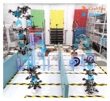
Figure 1: Demonstration of the proposed motion planning and control framework. HyFCQ navigates autonomously in the environment with hybrid flying-crawling motion. Video is available at https://youtu.be/G-84DAaqdJw

In this work, a motion planning and control framework is presented based on the structure and motion characteristics of HyFCQs, enabling the quadrotors to move through complex environments autonomously, as shown in Fig. 1. Firstly, the kinodynamic path-searching of the planner is optimized by incorporating crawling refinement to ensure the dynamic feasibility of trajectories. Then, a mapping of the control outputs from the flight autopilot to both crawling and flying modes is established. Furthermore, a motion state machine is proposed to classify the motion of the HyFCQ into seven distinct states. The state machine transitions the HyFCQ to the suitable motion state based on the varying states of the trajectory and manages its motion.

The contributions of our work are:

1. A terrestrial-aerial motion planner is proposed, which optimizes terrestrial path-searching with the crawling limitations of HyFCQs, thus enabling the generation of kinodynamically feasible hybrid trajectories.

2. A hierarchical motion controller that maps the control outputs of the flight autopilot to both crawling and flying modes is designed, ensuring precise and stable hybrid trajectory tracking.

3. A motion state machine that autonomously manages locomotion based on trajectory information is presented. We integrate the state machine with our planner and controller to achieve terrestrial-aerial hybrid navigation.

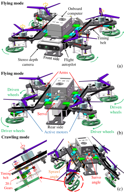
Figure 2: (a) The body core is equipped with sensing, computing, and control units. (b) The arms are equipped with actuation components consisting of reduction gears, timing belts, brushless motors, and wheels. They are linked to the servo mounted in the core. (c) The reduction gears transfer the torsion from the active motors to the rear wheels. The rear wheels convey the torque to the front wheels via timing belts. Symmetrical actuation of the sprawl angles on both sides is achieved through the servo.

II RELATED WORK

II-A Motion Planning

Although there is limited research dedicated to motion planning for HyFCQs, we can still reference planning methods designed for other terrestrial-aerial robots with different structures and motion modes. Fan et al. [11] addressed passive-wheeled quadrotors by employing the Hybrid A* method to search for paths. Their approach adds supplementary energy costs for aerial nodes, which guarantees that the planner prioritizes the search for terrestrial paths. Expanding upon [11], Zhang et al. [6] use kinodynamic searching and applied nonlinear optimization methods to refine the trajectory, which ensured its smoothness and its ability to navigate around obstacles. Furthermore, Zhang addressed the nonholonomic constraints of ground motion by optimizing the terrestrial trajectory, ensuring the feasibility of trajectories.

However, the above planners are not compatible with HyFCQs: 1) The crawling constraints of HyFCQs have not been integrated with the terrestrial search process, leading to dynamically infeasible trajectories in certain situations and large position errors. 2) The transition of motion modes requires some processing time, making it challenging to track the trajectories during the crawling-to-flying transition phase. Compared with the planner in [6], we impose constraints on kinodynamic path searching by using the crawling refinement of HyFCQs, ensuring the trajectory is dynamically feasible for HyFCQs. Furthermore, we propose a motion state machine that enables HyFCQs to smoothly transition between various motion states, thereby addressing the challenge of tracking terrestrial-aerial transition trajectories.

II-B Controller

Several works proposed controllers for passive-wheel quadrotors[6, 7]. In aerial motion, these controllers are similar to those used in traditional quadrotors. When in terrestrial motion, the driving method of passive-wheel quadrotors resembles that during aerial motion. Due to the substantial load-bearing capacity of the ground, the passive-wheel quadrotors require less thrust. In response to this characteristic, Zhang et al. [6] introduced an adaptive thrust control method for terrestrial motion. Building upon the principles of differential flatness, Pan et al. [7] developed a high-speed controller that amalgamates the dynamics of ground support and friction forces.

Unlike passive-wheel quadcopters, HyFCQ demonstrates a notable divergence in its propulsion methods between flying and crawling modes. During flight, its propulsion method is similar to conventional quadrotors’. Whereas in crawling mode, it relies on a gear reducer to transfer torque from the rear motors to the wheels. Its crawling motion model is similar to a two-wheeled differential-drive vehicle [12, 13, 14]. However, due to constraints of the electronic control system [9], HyFCQ lacks the capability to independently and freely control the rotation speed of each motor. Therefore, the controllers designed for passive-wheel quadrotors and two-wheeled differential-drive vehicles are not applicable to HyFCQ. Considering the utility of the flight autopilot for both crawling and flying, we propose a hierarchical controller to map the flight autopilot’s control outputs to various motion modes, thereby enabling terrestrial-aerial trajectory tracking.

III SYSTEM INTRODUCTION:

III-A Hardware Platform

The HyFCQ’s structure is based on Fcstar [10], with its principles illustrated in Fig. 2. It contains two primary components: the body core and the arms. The body core contains various electronic components such as flight autopilot, onboard computer, battery, stereo depth camera, and servo. The arms are distributed on both sides and equipped with brushless motors, propellers, reduction gears, timing belt mechanisms, and wheels. They are connected to the servos on the body core through ball joint linkage mechanisms. Our HyFCQ can switch between motion modes by the rotation of the servo motor.

HyFCQ has two modes of motion: flying mode and crawling mode. In flying mode, similar to conventional quadrotors, HyFCQ achieves propulsion through the rotation of the propellers driven by motors. In crawling mode, propulsion is facilitated through the rear motors. As the motors rotate, they drive the shafts beneath them to rotate and transfer torque to the rear wheels through the gears with a reduction ratio of 20:1. The torque from the rear wheels is transmitted to the front wheels via timing belt mechanisms, thereby achieving four-wheel drive.

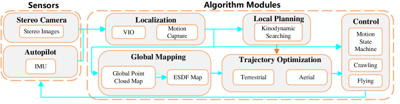
Figure 3: The proposed motion planning and control framework is integrated with the localization and mapping modules to form the autonomous navigation system. The sensors are responsible for the perception module, and the algorithm modules are responsible for localization, mapping, planning, and control modules

III-B Software architecture

We integrate the proposed planning and control framework with the mapping and localization module to establish a comprehensive autonomous navigation system, as shown in Fig. 3. Firstly, the current position and orientation can be obtained through Visual-Inertial Odometry (VIO) [15] or motion capture system. Subsequently, an Euclidean Signed Distance Field (ESDF) map is generated based on a pre-established global point cloud map. The planner generates the hybrid terrestrial-aerial trajectory based on position, orientation, and the map. The motion state machine can distinguish between different stages of the trajectory and select the appropriate controller for position tracking. During the motion, if the trajectory shows a takeoff or landing trend, the state machine governs the quadrotor’s transition between crawling mode and flying mode. Once the quadrotor completes the transition and reaches the desired state, the planner will replan the trajectory from the current position to the target point, ensuring the quadrotor reaches its destination.

IV TERRESTRIAL-AERIAL MOTION PLANNING

The proposed terrestrial-aerial motion planner is built on the Fast-Planner framework [16] which consists of three key components: kinodynamic path searching based on Hybrid-A* [18], non-uniform B-spline trajectory optimization based on the Euclidean Signed Distance Field (ESDF) map [19] and time adjustment method. We refer to the hybrid path-searching methods of [6, 11] which tend to search for a terrestrial path. In this work, we optimize the terrestrial path-searching module through yaw deviation refinement of crawling mode to ensure that there are no excessively large turning motions in the trajectories.

During crawling locomotion, due to the non-holonomic constraint and the limitations of the turning radius, it is necessary to maintain a relatively small disparity between the yaw angle of the trajectory and the present yaw angle of HyFCQ. Therefore, during the generation of trajectory primitives, we apply constraints to the trajectory with respect to the current yaw angle, which is denoted as $\psi_{t_{0}}^{W}$. The state space model for terrestrial search can be defined as follows:

$$\mathbf{\dot{x}}_{t}^{W} =\mathbf{R}_{d}^{-1}\mathbf{AR}_{d}\mathbf{x}_{t}^{W}+\mathbf{R}_{d}^{-1}\mathbf{Bu}_{t}^{B},$$ (1a)

$$\mathbf{R}_{d} =\left[\begin{matrix}\mathbf{R}&\bm{0}\\ \bm{0}&\mathbf{R}\\ \end{matrix}\right],\mathbf{A}=\left[\begin{matrix}\bm{0}&\mathbf{I}_{3}\\ \bm{0}&\bm{0}\\ \end{matrix}\right],\mathbf{B}=\left[\begin{array}[]{c}\bm{0}\\ \mathbf{I}_{3}\\ \end{array}\right],$$ (1d)

$$\mathbf{R} =\left[\begin{matrix}\cos\left(\psi_{t_{0}}^{W}\right)&\sin\left(\psi_{t_{0}}^{W}\right)&0\\ -\sin\left(\psi_{t_{0}}^{W}\right)&\cos\left(\psi_{t_{0}}^{W}\right)&0\\ 0&0&1\\ \end{matrix}\right],$$ (1e)

$$\psi_{t}^{W} =\tan^{-1}\frac{\left(\mathbf{p}_{t}^{W}\right)_{y}-\left(\mathbf{p}_{t_{0}}^{W}\right)_{y}}{\left(\mathbf{p}_{t}^{W}\right)_{x}-\left(\mathbf{p}_{t_{0}}^{W}\right)_{x}},$$ (1f)

where $\mathbf{x}_{t}^{W}=\left[\left(\mathbf{p}_{t}^{W}\right)^{\text{T}},\left(\mathbf{\dot{p}}_{t}^{W}\right)^{\text{T}}\right]^{\text{T}}\in\mathbb{R}^{6}$ , denoted as the state of the system in world coordinate. $\mathbf{p}_{t}^{W}=\left[\left(\mathbf{p}_{t}^{W}\right)_{x},\left(\mathbf{p}_{t}^{W}\right)_{y},\left(\mathbf{p}_{t}^{W}\right)_{z}\right]^{\text{T}}$, denoted as the position at time t. $\left(\mathbf{p}_{t}^{W}\right)_{x}$, $\left(\mathbf{p}_{t}^{W}\right)_{y}$ and $\left(\mathbf{p}_{t}^{W}\right)_{z}$ represent the components of $\mathbf{p}_{t}^{W}$ along x-y-z axis. $\mathbf{R}$ is the rotation matrix based on the initial state’s yaw $\psi_{t_{0}}^{W}$. It can transform the state from the world coordinate to the body coordinate. $\mathbf{u}_{t}^{B}=\left[\left(\mathbf{u}_{t}^{B}\right)_{x},\left(\mathbf{u}_{t}^{B}\right)_{y},\left(\mathbf{u}_{t}^{B}\right)_{z}\right]^{\text{T}}$ is control input in the body coordinate. Then, the state transition result in the body coordinate is calculated based on the input $\mathbf{u}_{t}^{B}$. Finally, the result is transformed into the world coordinate by premultiplying $\mathbf{R}_{d}^{-1}$. The solution for the state equation can be expressed as:

$$\mathbf{x}_{t}^{W}=e^{\mathbf{R}_{d}^{-1}\mathbf{AR}_{d}t}\mathbf{x}_{t_{0}}^{W}+\int_{0}^{t}{e^{\mathbf{R}_{d}^{-1}\mathbf{AR}_{d}\left(t-\tau\right)}\mathbf{R}_{d}^{-1}\mathbf{Bu}_{\tau}^{B}d\tau}.$$ (2)

To constrain yaw angle deviation, we constrain the size of $\left(\mathbf{u}_{t}^{B}\right)_{x}$ relative to $\left(\mathbf{u}_{t}^{B}\right)_{y}$ and discretize each dimension of the control input. We set range of $\left(\mathbf{u}_{t}^{B}\right)_{x}$ as $\left\{\left(\frac{1}{r}+\alpha\right)u_{\max},\left(\frac{2}{r}+\alpha\right)u_{\max},...,u_{\max}\right\}$, and range of $\left(\mathbf{u}_{t}^{B}\right)_{y,z}$ as $\left\{-u_{\max},-\frac{r-1}{r}u_{\max},...,\frac{r-1}{r}u_{\max},...,u_{\max}\right\}$. Where $\alpha$ is a variable ranging from 0 to 1 and is used to limit the maximum yaw deviation. When $\alpha$ is increased, the maximum yaw deviation decreases. However, an excessively large value for $\alpha$ may result in path-searching failures. The appropriate value of $\alpha$ should be determined through experimental analysis.

If the z-axis value in the world coordinate, whether derived from a search procedure or state estimation, surpasses a predefined threshold, the planner will work with aerial searching. In this scenario, the quadrotor is free from non-holonomic constraints. So the state equation is expressed as:

$$\mathbf{x}_{t}^{W}=e^{\mathbf{A}t}\mathbf{x}_{t_{0}}^{W}+\int_{0}^{t}{e^{\mathbf{A}\left(t-\tau\right)}\mathbf{Bu}_{\tau}^{W}d\tau},$$ (3)

where $\mathbf{u}_{t}^{W}$ denoted as the control input in the world coordinate. Each dimension $\left[-u_{\max},u_{\max}\right]$ is discretized as $\left\{-u_{\max},-\frac{r-1}{r}u_{\max},...,\frac{r-1}{r}u_{\max},...,u_{\max}\right\}$.

When the motion planning is complete, a desired state in the world frame is selected from the generated trajectory based on the current timestamp and sent to the controller. The desired state contains position, velocity, and yaw angle ($\left[\left(\mathbf{p}_{t}^{W}\right)_{d},\left(\mathbf{v}_{t}^{W}\right)_{d},\left(\psi_{t}^{W}\right)_{d}\right]^{\text{T}}$). $\left(\psi_{t}^{W}\right)_{d}$ is set to be parallel with the desired velocity.

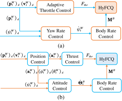
Figure 4: (a) The controller for crawling mode. (b) The controller for flying mode.

V HIERARCHICAL MOTION CONTROLLER

The driving methods for the flying mode and crawling mode of HyFCQs display significant differences. In the flying mode, HyFCQs are actuated similarly to standard quadrotors. In the crawling mode, the rear motors transmit torque to the wheels through 20:1 reduction gears for forward motion. Steering is accomplished by creating a speed differential between the active motors on both sides.

In this article, we use the PX4 open-source firmware[20] as the flight autopilot firmware. The PX4 firmware calculates the rotational speed of each motor by receiving variables such as throttle thrust $F_{thr}$ (a normalized value ranging from 0 to 1) and body angular rates $\mathbf{\dot{\Theta}}_{t}^{B}$. According to this feature, a hierarchical controller is proposed to independently control the motion in both crawling and flying modes.

This controller maps throttle thrust and body angular rates to different motion modes. In flying mode, adjusting parameter $F_{thr}$ influences the flight altitude, while manipulating the body angular rates results in changes to the orientation of the quadrotors. In crawling mode, adjusting parameter $F_{thr}$ serves to modify the forward velocity, whereas manipulating the body angular rates results in alterations to the turning radius.

The observed state at time $t$ is acquired through the localization module, denoted as $\mathbf{\hat{X}}_{t}^{W}$. $\mathbf{\hat{X}}_{t}^{W}=\left[\mathbf{\hat{p}}_{t}^{W},\mathbf{\hat{v}}_{t}^{W},\mathbf{\hat{\Theta}}_{t}^{W},\mathbf{\hat{\dot{\Theta}}}_{t}^{W}\right]^{\text{T}}$, respectively correspond to position, velocity, orientation, and angular rates. The orientation $\mathbf{\hat{\Theta}}_{t}^{W}$ and angular rates $\mathbf{\hat{\dot{\Theta}}}_{t}^{W}$ are parameterized in the $X-Y-Z$ Euler angle sequence. $\mathbf{\hat{\Theta}}_{t}^{W}=\left[\mathbf{\hat{\phi}}_{t}^{W},\mathbf{\hat{\theta}}_{t}^{W},\hat{\psi}_{t}^{W}\right]^{\text{T}}$, $\mathbf{\hat{\dot{\Theta}}}_{t}^{W}=\left[\mathbf{\hat{\dot{\phi}}}_{t}^{W},\mathbf{\hat{\dot{\theta}}}_{t}^{W},\hat{\dot{\psi}}_{t}^{W}\right]^{\text{T}}$. The desired state includes $\left(\mathbf{p}_{t}^{W}\right)_{d}$, $\left(\mathbf{v}_{t}^{W}\right)_{d}$, and $\left(\psi_{t}^{W}\right)_{d}$ is obtained from the trajectory generated by our planner.

V-A Crawling Controller

The crawling controller is illustrated in Fig. 4(a). In crawling mode, the pivotal challenge is how to control the yaw rate $\dot{\psi}_{t}^{W}$ and throttle thrust $F_{thr}$ to reduce the position error along x-axis and y-axis.

V-A1 Yaw Rate Control

Assuming a level ground, it follows that the z-axis in both the world coordinate system and the body coordinate system run in parallel and in the same direction. In this context, the yaw rate $\dot{\psi}_{t}^{W}$ in the world coordinate system and $\dot{\psi}_{t}^{B}$ in the body coordinate system are identical. We account for the current yaw angle of the quadrotor, the desired yaw angle, and the deviation between the current position and the desired position in the trajectory. The calculation of $\dot{\psi}_{t}^{W}$ is defined as:

$$\dot{\psi}_{t}^{W}=K_{y}\left[\lambda_{d}\left(\psi_{t}^{W}\right)_{d}^{e}+\lambda_{p}\left(\psi_{t}^{W}\right)_{p}^{e}\right],$$ (4)

where $K_{y}$ represents the proportional gain. $\left(\psi_{t}^{W}\right)_{d}^{e}$ is the deviation between the desired yaw angle in the trajectory and the current yaw angle, and $\left(\psi_{t}^{W}\right)_{d}^{e}=\left(\psi_{t}^{W}\right)_{d}-\hat{\psi}_{t}^{W}$. $\left(\psi_{t}^{W}\right)_{p}^{e}$ signifies the deviation between the expected angular displacement due to position error and the current yaw angle, and $\left(\psi_{t}^{W}\right)_{p}^{e}=tan^{-1}\frac{\left(\mathbf{p}_{t}^{W}\right)_{y}^{e}}{\left(\mathbf{p}_{t}^{W}\right)_{x}^{e}}-\hat{\psi}_{t}^{W}$. Where the position error $\left(\mathbf{p}_{t}^{W}\right)^{e}$ is defined as $\left(\mathbf{p}_{t}^{W}\right)^{e}=\left(\mathbf{p}_{t}^{W}\right)_{d}-\mathbf{\hat{p}}_{t}^{W}$ . $\left(\mathbf{p}_{t}^{W}\right)_{x}^{e}$ and $\left(\mathbf{p}_{t}^{W}\right)_{y}^{e}$ respectively represent the value of $\left(\mathbf{p}_{t}^{W}\right)^{e}$ along x-axis and y-axis. Variables $\lambda_{d}$ and $\lambda_{p}$ serve as weight parameters, and their values are adjusted based on specific circumstances, with the constraint that $\lambda_{d}+\lambda_{p}=1$. When the norm of $\left(\mathbf{p}_{t}^{W}\right)^{e}$ exceeds a certain threshold, it means a large positional error. In this situation when calculating $\dot{\psi}_{t}^{W}$, greater consideration should be given to the yaw angle error generated by the position error. Consequently, there is an increase in $\lambda_{p}$ and a decrease in $\lambda_{d}$. By the same principle, when the norm of $\left(\mathbf{p}_{t}^{W}\right)^{e}$ falls below a specific threshold, it indicates a relatively minor position error, and the reference should shift more towards the desired yaw from the trajectory. This leads to an increase in $\lambda_{d}$ and a decrease in $\lambda_{p}$.

V-A2 Adaptive Throttle Control

In crawling mode, the forward velocity $V$ is determined by the throttle thrust $F_{thr}$ , and $F_{thr}$ varies directly with forward speed $V$. We establish multiple sets of throttle and record the corresponding forward velocities. Through a linear regression approach, we derive the relationship between $V$ and $F_{thr}$:

$$V=6.838F_{thr}+0.0016.$$ (5)

$V_{t}$, the forward velocity at time t can be calculated as:

$$V_{t}=\lVert\left(\mathbf{v}_{t}^{W}\right)_{d}+K_{p}\left(\mathbf{p}_{t}^{W}\right)^{e}\rVert,$$ (6)

where $\left(v_{t}^{W}\right)_{d}$ is the desired velocity in the trajectory. $K_{p}$ is the proportional gain for the position error. When the position error is substantial, this gain facilitates the rapid convergence of $V_{t}$ to the desired value. By combining (5) with (6), $F_{thr}$ can be calculated:

$$F_{thr}=K_{thr}\frac{\left(V_{t}-0.00162073\right)}{6.837577},$$ (7)

$K_{thr}$ is the proportional gain, and increasing its value appropriately can accelerate the response of motion.

In crawling mode, the propellers generate thrust in both the y-axis and z-axis of the quadrotor’s body. Excessive thrust can lead to significant lateral deviations, reduced friction with the ground, and overly rapid crawling speeds. In order to prevent the issues mentioned above, we impose restrictions on the maximum value of $F_{thr}$.

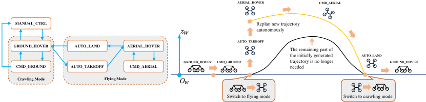
Figure 5: Left) The system architecture of the motion state machine. Right) The schematic diagram of the motion state machine collaborating with the planner to achieve autonomous hybrid terrestrial-aerial navigation

V-B Flying Controller

The flying controller is shown in Fig. 4(b). The position controller calculates the desired acceleration $\left(\mathbf{a}_{t}^{W}\right)_{d}$, desired roll angle $\left(\phi_{t}^{W}\right)_{d}$, and desired pitch angle $\left(\theta_{t}^{W}\right)_{d}$ based on the error between the reference trajectory and the current position and velocity [21]. The thrust controller determines $\left(\mathbf{a}_{t}^{W}\right)_{d}$ based on $F_{thr}$ . The attitude controller generates angular rates based on the desired attitude angles. These angular rates then pass through the body rate controller to produce the desired torque $\mathbf{M}^{B}$. Finally, the PX4 firmware calculates the rotational speed of each motor based on $F_{thr}$ and $\mathbf{M}^{B}$.

VI Motion State Machine

There are some problems when HyFCQs transition between various states and modes: 1) HyFCQs have different driving and control methods for crawling and flying. The challenge lies in autonomously selecting the suitable motion mode based on the evolving states of the trajectory. 2) The motion of the morphing mechanism requires a certain duration during mode transition, leading to difficulties in the tracking desired trajectory during the take-off phase. 3) In the mode transition process, the motors must remain stationary to prevent loss of control. In order to achieve appropriate transitions between motion states autonomously, we devise this motion state machine for motion state management.

TABLE I: Explanation Of Motion States

State	Explanation
MANUAL_CONTROL	Remote control of quadrotor motion.
GROUND_HOVER	Maintaining stationary on the ground, awaiting the emergence of the trajectory.
CMD_GROUND	Automatically transitioning into this state when the ground-phase trajectory becomes available for position tracking.
AUTO_TAKEOFF	Autonomously taking off to a certain altitude.
AERIAL_HOVER	Hovering at a certain location in the air, awaiting the appearance of a trajectory.
CMD_AERIAL	Automatically transitioning into this state when the aerial-phase trajectory becomes available for position tracking.
AUTO_LAND	Autonomously landing and ceasing motor rotation upon a successful landing.

This state machine classifies the motion into seven distinct states: MANUAL_CONTROL, GROUND_HOVER, CMD_GROUND, AUTO_TAKEOFF, AERIAL_HOVER, CMD_AERIAL, AUTO_LAND. The functions of these states are detailed in TABLE I, and these states can transition under certain conditions. This state machine can switch motion modes based on the different phases of the trajectory, as shown in Fig. 5.

When generating a hybrid trajectory, HyFCQ transitions from GROUND_HOVER to CMD_GROUND, autonomously tracking the terrestrial trajectory with the crawling controller. As the trajectory indicates an upward trend, the state machine commands HyFCQ to shift from crawling mode to flying mode. The quadrotor ceases tracking the remaining trajectories and enters AUTO_TAKEOFF state for automatic takeoff.

After reaching the specified altitude, HyFCQ enters AUTO_HOVER and plans a new trajectory. Then, the quadrotor enters CMD_AERIAL for autonomous flight. As the trajectory descends, HyFCQ enters AUTO_LAND for the descent to the ground. Finally, HyFCQ returns to crawling mode and awaits the next trajectory.

At the outset of the taking-off process, precise throttle thrust $F_{thr}$ can be calculated through the formula:

$$F_{thr}=\frac{\hat{a}_{z}}{k_{f}},$$ (8)

where $\hat{a}_{z}$ represents the observed z-axis acceleration in the world coordinate system, and $k_{f}$ is the throttle thrust coefficient. To prevent sudden surges during quadrotor takeoff, we preset a value $F_{pre\_thr}$ slightly lower than the $F_{thr}$ of stable hover.

In practical environments, $F_{thr}$ is influenced by air density, battery level, propeller type, and other factors. Therefore, it is essential to determine an accurate value for $k_{f}$ . We use a forgetting factor recursive least-squares algorithm to calculate $k_{f}$ [22]. The algorithm is expressed as:

$$\left(k_{f}\right)_{k+1}=\left(k_{f}\right)_{k}+\frac{P_{k}\left(F_{thr}\right)_{k+1}}{\rho+\left(F_{thr}\right)_{k+1}\left(F_{thr}\right)_{k+1}P_{k}}e_{k+1},$$ (9)

$$P_{k+1}=\frac{P_{k}}{\rho}\left[1-\frac{\left(F_{thr}\right)_{k+1}\left(F_{thr}\right)_{k+1}P_{k}}{\rho+\left(F_{thr}\right)_{k+1}\left(F_{thr}\right)_{k+1}P_{k}}\right],$$ (10)

combining the expression (8) with (9) and (10), we can iteratively refine $k_{f}$. Error term $e_{k+1}=\left(\hat{a}_{z}\right)_{k+1}-\left(F_{thr}\right)_{k+1}\left(k_{f}\right)_{k}$ . Where $\rho$ is the forgetting factor, which falls within the range of 0.98 to 1. $P_{k}$ is covariance and is used to describe the uncertainty associated with the estimated parameters.

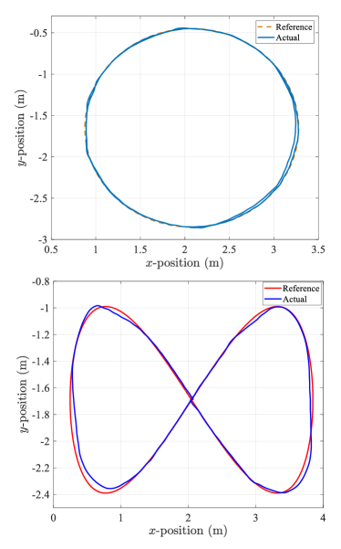
Figure 6: Top) The circular trajectory tracking. Botton) The figure-eight trajectory tracking.

VII Experiments

To validate the proposed methods, we developed a HyFCQ platform. Considering strength and weight, we use carbon fiber panels in the construction of the body core and arms. For components such as rotating joints, wheels, and the shell for the onboard computer, we use 3D printing with polylactic acid (PLA).

The total weight of HyFCQ is 1.6 kg including a 3300 mAh - 14.8 V battery that weighs 303 g. In flying mode, its wheelbase measures 200 mm on the lateral axis and 210 mm on the longitudinal axis. Upon the transition to crawling mode, the overall width reduces from 320 mm to 260 mm.

VII-A Terrestrial trajectory tracking

Aiming at confirming the effectiveness of the crawling controller, we conduct tests using circular and figure-eight trajectories. The evaluation criteria for trajectory tracking performance are the average tracking error $E_{a}$ and the maximum tracking error $E_{m}$. The circular has a radius of 1.2 meters, while the figure-eight has a longitudinal length of 3.6 meters and a lateral width of 1.4 meters.

Tracking results are shown in the Table II and Fig. 6. It can be seen that the proposed controller achieves stable tracking of the terrestrial trajectories effectively.

TABLE II: The Result Of Trajectory Tracking

Trajectory	$v_{\max}(m/s)$	$E_{a}(m)$	$E_{m}(m)$
Circular	0.8	0.0460	0.0469
Eight-Shaped	1.0	0.0481	0.0640

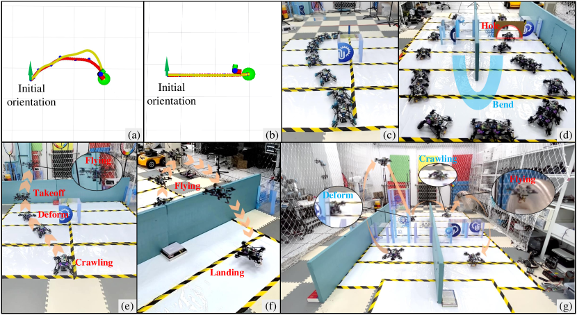
Figure 7: The experiments of autonomous navigation. (a) By considering the initial orientation of HyFCQ, our planner generates trajectories with gradual yaw angle changes that are dynamically feasible for HyFCQ. (b) The planner without the constraints of HyFCQ generates a direct trajectory from the starting point to the endpoint, which is dynamically infeasible. (c) HyFCQ crawls around an obstacle. (d) HyFCQ traverses a passage with rectangular blocks, a U-shaped bend, and a semi-circular hole. (e) HyFCQ crawls around an obstacle and flies over a wall. (f) The scenario is the second view of Fig. 10(e). (g) HyFCQ moves through the passage with multiple blocks.

VII-B Comparison of Terrestrial Trajectory Planning

To demonstrate the adaptability of our planner under the crawling constraints of HyFCQs, we compare it with Zhang’s method [6], which lacks consideration for these constraints. As shown in Fig. 7(b), the trajectory generated by Zhang’s planner exhibits a significant deviation from the initial orientation, making it evidently dynamically infeasible. This results in substantial position errors and may lead to failure in reaching the goal. By contrast, the proposed planner generates a trajectory that features a gradual change in yaw angle, aligning it with the current orientation. The proposed approach results in a smoother transition of yaw angle, which is advantageous for position tracking, as shown in Fig. 7(a). This comparison indicates the superior adaptability and performance of our planner.

VII-C Terrestrial trajectory planning and autonomous tracking

HyFCQs feature compact design, stable propulsion, and adjustable dimensions, enabling them to adapt to constrained environments, such as narrow passages and tight holes. In this experiment, we set up scenarios including rectangular blocks, a U-shaped bend, and a semi-circular hole to evaluate the navigation ability of HyFCQs in these terrains.

The results are shown in Figs. 7(c) and 7(d). Firstly, the whole motion remains in a land-based state which proves our trajectories save energy and avoid mode switching as much as possible. Then, the HyFCQ tracks the trajectories by the crawling controller, moving through the passage with various obstacles. Experimental outcomes validate the remarkable performance of the proposed planner and crawling controller in constrained environments.

VII-D Hybrid terrestrial-aerial navigation

In this experiment, two different scenarios are given for testing the entire navigation system. In these scenarios, walls or multiple blocks are present, requiring HyFCQ to transition to flying mode when necessary.

In the first scenario, we place a rectangular block and a wall in front of HyFCQ, as shown in Figs 7(e) and 7(f). Firstly, the quadrotor successfully crawls around the rectangular cuboid. Then, if the trajectory shows the taking-off trend, HyFCQ will seamlessly transition into flying mode and autonomously ascend to a hovering state. After entering a stable hover, HyFCQ autonomously replans the trajectory based on the current position. Then, HyFCQ flies over the wall and reaches the destination. After that, it automatically lands and waits for the next trajectory.

In the second scenario, as shown in Fig. 7(g), there is a passage with multiple blocks which brings challenges to motion planning and state transition. It turns out that the HyFCQ safely traverses the passage in crawling-flying integrated locomotion, which reveals that the proposed approach in this paper is effective and practical.

VIII CONCLUSION

In this study, we propose a motion planning and control framework specifically designed to accommodate the unique motion characteristics of HyFCQs. To optimize terrestrial path-searching of the hybrid motion planner, we incorporate crawling refinement to generate dynamically feasible trajectories. A hierarchical motion controller is built upon the control input-output characteristics of the flight autopilot, enabling hierarchical control of both crawling and flying modes by mapping the execution generated by the same input to different motion modes. Additionally, we propose a motion state machine to manage locomotions by various phases of the trajectory. Furthermore, we integrate the framework with localization and mapping modules to validate the effectiveness of the entire navigation system.

In the future, we plan to incorporate motion mode switching constraints into the transition trajectories for both takeoff and landing, enhancing the speed and smoothness of the HyFCQs during these critical phases. We also need to solve the problem with turning radius limits for HyFCQs to enhance the flexibility of HyFCQs in crawling mode.

References

- [1] R. B¨ahnemann, D. Schindler, M. Kamel, R. Siegwart, and J. Nieto, “A decentralized multi-agent unmanned aerial system to search, pick up, and relocate objects,” in Proceedings of2017 IEEE International Symposium on Safety, Security and Rescue Robotics (SSRR), p. 8088150, IEEE, 2017.
- [2] A.-a. Agha-mohammadi, N. K. Ure, J. P. How, and J. Vian, “Health aware stochastic planning for persistent package delivery missions using quadrotors,” in 2014 IEEE/RSJ International Conference on Intelligent Robots and Systems, pp. 3389–3396, IEEE, 2014.
- [3] Q. Quan, Introduction to Multicopter Design and Control. Berlin, Germany: Springer, 2017.
- [4] L. Quan, L. Han, B. Zhou, S. Shen, and F. Gao, “Survey of UAV motion planning,” IET Cyber- Syst. Robot., vol. 2, no. 1, pp. 14–21, 2020.
- [5] T Wu, Y Zhu, L Zhang, J Yang and Y Ding, “Unified Terrestrial/Aerial Motion Planning for HyTAQs via NMPC,” IEEE Robot. Automat. Lett., vol. 8, no. 2, pp. 1085-1902, 2023.
- [6] R. Zhang, Y. Wu, L. Zhang, C. Xu, and F. Gao, “Autonomous and adaptive navigation for terrestrial-aerial bimodal vehicles,” IEEE Robot. Automat. Lett., vol. 7, no. 2, pp. 3008–3015, Apr. 2022.
- [7] N. Pan, J. Jiang, R. Zhang, C. Xu, and F. Gao, ”Skywalker: A Compact and Agile Air-Ground Omnidirectional Vehicle,” IEEE Robotics and Automation Letters, vol. 8, no. 5, pp. 2534-2541, May. 2023.
- [8] S. Mintchev and D. Floreano, “A multi-modal hovering and terrestrial robot with adaptive morphology,” in Proc. 2nd Int. Symp. Aerial Robot., 2018.
- [9] M. Nir, and D. Zarrouk. ”Flying star, a hybrid crawling and flying sprawl tuned robot,” in Proc. IEEE Int. Conf. Robot. Automat., 2019, pp. 5302-5308.
- [10] N. B. David and D. Zarrouk, “Design and analysis of FCSTAR, a hybrid flying and climbing sprawl tuned robot,” IEEE Robot. Automat. Lett., vol. 6, no. 4, pp. 6188–6195, Oct. 2021.
- [11] D. D. Fan, R. Thakker, T. Bartlett, M. B. Miled, L. Kim, E. Theodorou, and A.-a. Agha-mohammadi, “Autonomous hybrid ground/aerial mobility in unknown environments,” in 2019 IEEE/RSJ International Conference on Intelligent Robots and Systems (IROS). IEEE, 2019, pp. 3070–3077.
- [12] L. Caracciolo, A. De Luca and S. Iannitti, ”Trajectory Tracking Control of a Four-wheel Differentially Driven Mobile Robot,” in Proc. IEEE Int. Conf. Robot. Automat., 1999, pp. 2632-2638.
- [13] M. Ahmad, V. Polotski and R. Hurteau, ”Path tracking control of tracked vehicles,” in Proc. IEEE Int. Conf. Robot. Automat., 2000, pp. 2938-2943.
- [14] S. Blažič, ”A novel trajectory-tracking control law for wheeled mobile robots,” Robotics and Autonomous Systems., vol. 59, no. 11, pp. 1001-1007, 2011.
- [15] T Qin, J Pan, S Cao and S Shen, “A general optimization-based framework for local odometry estimation with multiple sensors,” arXiv preprint arXiv:1901.03638, 2019.
- [16] B. Zhou, F. Gao, L. Wang, C. Liu, and S. Shen, “Robust and efficient quadrotor trajectory generation for fast autonomous flight,” IEEE Robotics and Automation Letters, vol. 4, no. 4, pp. 3529–3536, 2019.
- [17] X. Zhou, Z. Wang, H. Ye, C. Xu, and F. Gao, “Ego-planner: An esdffree gradient-based local planner for quadrotors,” IEEE Robotics and Automation Letters, vol. 6, no. 2, pp. 478–485, 2021
- [18] D. Dolgov, S. Thrun, M. Montemerlo, and J. Diebel, “Path planning for autonomous vehicles in unknown semi-structured environments,” Int. J. Robot. Res., vol. 29, no. 5, pp. 485–501, 2010.
- [19] V. Usenko, L. von Stumberg, A. Pangercic, and D. Cremers, “Real-time trajectory replanning for MAVs using uniform b-splines and a 3d circular buffer,” in Proc. IEEE/RSJ Int. Conf. Intell. Robots Syst., 2017, pp. 215–222.
- [20] L. Meier, D. Honegger and M. Pollefeys, ”PX4: A Node-Based Multithreaded Open Source Robotics Framework for Deeply Embedded Platforms,” in Proc. IEEE Int. Conf. Robot. Automat., 2015, pp. 6235-6240.
- [21] D. Mellinger and V. Kumar, “Minimum snap trajectory generation and control for quadrotors,” in 2011 IEEE international conference on robotics and automation., IEEE, 2011, pp. 2520–2525.
- [22] C. Paleologu, J. Benesty, and S. Ciochina, “A robust variable forgetting factor recursive least-squares algorithm for system identification,” IEEE Signal Process. Lett., vol. 15, no. 9, pp. 597–600, Oct. 2008.