Efficient Reactive Synthesis
Using Mode Decomposition

Abstract

Developing critical components, such as mission controllers or embedded systems, is a challenging task. Reactive synthesis is a technique to automatically produce correct controllers. Given a high-level specification written in LTL, reactive synthesis consists of computing a system that satisfies the specification as long as the environment respects the assumptions. Unfortunately, LTL synthesis suffers from high computational complexity which precludes its use for many large cases.

A promising approach to improve synthesis scalability consists of decomposing a safety specification into a smaller specifications, that can be processed independently and composed into a solution for the original specification. Previous decomposition methods focus on identifying independent parts of the specification whose systems are combined via simultaneous execution.

In this work, we propose a novel decomposition algorithm based on modes, which consists on decomposing a complex safety specification into smaller problems whose solution is then composed sequentially (instead of simultaneously). The input to our algorithm is the original specification and the description of the modes. We show how to generate sub-specifications automatically and we prove that if all sub-problems are realizable then the full specification is realizable. Moreover, we show how to construct a system for the original specification from sub-systems for the decomposed specifications. We finally illustrate the feasibility of our approach with multiple cases studies using off-the-self synthesis tools to process the obtained sub-problems.

1 Introduction

Reactive synthesis [11] is the problem of constructing a reactive system automatically from a high-level description of its desired behavior. A reactive system interacts continuously with an uncontrollable external environment [12]. The specification describes both the assumptions that the environment is supposed to follow and the goal that the system must satisfy. Reactive synthesis guarantees that every execution of the system synthesized satisfies the specification as long as the environment respects the assumptions.

Linear-Time Temporal Logic (LTL) [47] is a widely used formalism in verification [44] and synthesis [48] of reactive systems. Reactive synthesis can produce controllers which are essential for various applications, including hardware design [6] and control of autonomous robotic systems [36, 17].

Many reactive synthesis tools have been developed in recent years [25, 19] in spite of the high complexity of the synthesis problem. Reactive synthesis for full LTL is 2EXPTIME-complete [48], so LTL fragments with better complexity have been identified. For example, GR(1)—general reactivity with rank 1—enjoys an efficient (polynomial) symbolic synthesis algorithm [6]. Even though GR(1) can express the safety fragment of LTL considered in this paper, translating our specifications into GR(1) involves at least an exponential blow-up in the worst case [32]. Better scalable algorithms for reactive synthesis are still required [38].

Model checking, which consists on deciding whether a given system satisfies the specification, is an easier problem than synthesis. Compositional approaches to model checking break down the analysis into smaller sub-tasks, which significantly improve the performance. Similarly, in this paper we aim to improve the scalability of reactive synthesis introducing a novel decomposition approach that breaks down the original specification into multiple sub-specifications.

There are theoretical compositional approaches [21, 39], and implementations that handle large conjunctions [4, 13, 46]. For instance, Lisa [4] has successfully scaled synthesis to significant conjunctions of LTL formulas over finite traces (a.k.a. LTL_f[14]). Lisa is further extended to handling prominent disjunctions in Lydia [13]. These modular synthesis approaches rely heavily on the decomposition of the specification into simultaneous sub-specifications [24]. However, when sub-specifications share multiple variables, these approaches typically return the exact original specification, failing to generate smaller decompositions.

We tackle this difficulty by introducing a novel decomposition algorithm for safety LTL specifications. We chose the safety fragment of LTL [52, 40] because it is a fundamental requirement language in many safety-critical applications. Extending our approach to larger temporal fragments of LTL is future work.

To break down a specification we use the concept of mode. A mode is a sub-set of the states in which the system can be during its execution which is of particular relevance for the designer of the system. At any given point in the execution, the system is in a single mode, and during an execution the system can transition between modes. In requirement design, the intention of modes is often explicitly expressed by the requirement engineers as a high-level state machine. Using LTL reactive synthesis these modes are boiled down into additional LTL requirements , which are then processed with the rest of the specification. In this paper, we propose to exploit modes to decompose the specification into multiple synthesis sub-problems.

Most previous decomposition methods [33, 24] break specifications into independent simultaneous sub-specifications whose corresponding games are solved independently and the system strategies composed easily. In contrast, we propose sequential games, one for each mode. For each mode decomposition, we restrict the conditions under which each mode can “jump” into another mode based on the initial conditions of the arriving mode. From the point of local analysis of the game that corresponds to a mode, jumping into another mode is permanently winning. We show in this paper that our decomposition approach is sound—meaning that given a specification, system modes and initial conditions—if all the sub-specifications generated are realizable, then the original specification is realizable. Moreover, we show a synthesis method that efficiently constructs a system for the full specification from systems synthesized for the sub-specifications. An additional advantage of our method is that the automaton that encodes the solution is structured according to the modes proposed, so it is simpler to understand by the user.

1.0.1 Related Work.

The problem of reactive synthesis from temporal logic specifications has been studied for many years [20, 48, 2, 6]. Given its high complexity (2EXPTIME-complete [48]) easier fragments of LTL have been studied. For example, reactive synthesis for GR(1) specifications can be solved in polynomial time [6]. Safety-LTL has attracted significant interest due to its algorithmic simplicity compared to general LTL synthesis [53], but the construction of deterministic safety automaton presents a performance bottleneck for large formulas.

For the model-checking problem, compositional approaches improve the scalability significantly [50], even for large formulas. Remarkably, these approaches break down the analysis into smaller sub-tasks [48]. For model-checking, Dureja and Rozier [18] propose to analyze dependencies between properties to reduce the number of model-checking tasks. Recently, Finkbeiner et al. [24] adapt this idea to synthesis, where the dependency analysis is based on controllable variables, which makes the decomposition impossible when the requirements that form the specification share many system (controlled) variables. We propose an alternative approach for dependency analysis in the context of system specification, by leveraging the concept of mode to break down a specification into smaller components. This approach is a common practice in Requirements Engineering (RE) [28, 27] where specifications typically contain a high-level state machine description (where states are called modes) and most requirements are specific to each mode. Furthermore, this approach finds widespread application in various industries, employing languages such as EARS [45] and NASA’s FRET language [26]. Recently, a notion of context is introduced by Mallozi et al [43] in their recent work on assume-guarantee contracts. Unlike modes, contexts depend solely on the environment and are not part of the elicitation process or the system specification.

Software Cost Reduction (SCR) [31, 28, 27] is a well-establish technique that structures specifications around mode classes and modes. A mode class refers to internally controlled variables that maintain state information with a set of possible values known as modes.

We use modes here provided by the user to accelerate synthesis, exploiting that in RE modes are comonly provided by the engineer during system specification. Recently, Balachander et al. [3] proposed a method to assist the synthesis process by providing a sketch of the desired Mealy machine, which can help to produce a system that better aligns with the engineer’s intentions. This approach is currently still only effective for small systems, as it requires the synthesis of the system followed by the generation of example traces to guide the search for a reasonable solution. In contrast our interest is in the decomposition of the synthesis process in multiple synthesis sub-tasks.

Other compositional synthesis approaches aim to incrementally add requirements to a system specification during its design [39]. On the other hand, [23] and [24] rely extensively on dropping assumptions, which can restrict the ability to decompose complex real-world specifications.

2 Motivating Example

We illustrate the main ideas of our decomposition technique using the following running example of a counter machine (CM) with a reset. The system must count the number of ticks produced by an external agent, unless the reset is signaled—also by the environment—in which case the count is restarted. When the count reaches a specific limit, the count has to be restarted as well and an output variable is used to indicate that the bound has been reached. Fig. 1 shows a specification for this system with a bound of $20$. This example is written in TLSF (see [34]), a well-established specification language for reactive synthesis, which is widely used as a standard language for the synthesis competition, SYNTCOMP [1].

⬇

PARAMETERS { N = 20;}

INPUTS {reset;start;} OUTPUTS {counter[N+1];trigger;}

INITIALLY{ (!reset && !start);} ASSUMPTIONS{ G !(reset && start);}

PRESET{counter[0] && (&&[1 <= i <=N]!counter[i]);}

DEFINITIONS {

mutual(b) = G ||[0 <= i < n](b[i] && &&[j IN {0, 1 .. (n-1)} (\) {i}] !b[j]);}}

GUARANTEES

mutual(counter); G (reset $\rightarrow$ X counter[0]);

G ((counter[0] && start) $\rightarrow$ X (counter[1] || reset));

G ((counter[1] && !reset) $\rightarrow$ X (counter[2] || reset));

...

G ((counter[N-1] && !reset) $\rightarrow$ X (counter[N] || reset));

G (counter[N] $\rightarrow$ X counter[0]);

G (counter[N] $\rightarrow$ trigger); G (!counter[N] $\rightarrow$ !trigger);

Figure 1: Counter machine specification.

Even for this simple specification, all state-of-the-art synthesis tools from the synthesis competition SYNTCOMP [1], including Strix [46], are unable to produce a system that satisfies CM.

Recent decomposition techniques [24, 33] construct a dependency graph considering controllable variable relationships, but fail to decompose this specification due to the mutual dependencies among output variables. Our technique breaks down this specification into smaller sub-specifications, grouping the counter machine for those states with counter value $1$ and $2$ in a mode, states with counter $3$ and $4$ in a second mode, etc, as follows:

Smaller controllers are synthesized independently, which can be easily combined to satisfy the original specification 1. In the example, we group the states in pairs for better readability, but it is possible to use larger sizes. In fact, for $N=20$ the optimal decomposition considers modes that group four values of the counter (see Section 5). The synthesis for each mode is efficient because in a given mode we can ignore those requirements that involve valuations that belong to other modes, leading to smaller specifications.

⬇

// common part to all projections.

INPUTS {reset;start;} INITIALLY (!reset && !start); ASSUMPTIONS G !(reset && start);

[Projection under m1]

OUTPUTS {counter_0, counter_1; trigger; $\emph{jump}_{2}$; $s_{\LTLcircle\varphi}$; done}

GUARANTEES

G (!done $\rightarrow$ (counter_0 || counter_1));

G (!done $\rightarrow$ (reset $\rightarrow$ X counter_0));

G (!done $\rightarrow$ (counter_0 && start) $\rightarrow$ X (counter_1 || reset));

G (!done $\rightarrow$ ((counter_1 && !reset) $\rightarrow$ $s_{\LTLcircle\varphi}$));

G (!done $\rightarrow$ ($s_{\LTLcircle\varphi}$ && !done) $\rightarrow$ X FALSE);

G (!done $\rightarrow$ !trigger);

G (done $\rightarrow$ X done);

G ($\emph{jump}_{2}$ $\rightarrow$ X done);

G (!$\emph{jump}_{2}$ $\rightarrow$ (!done $\rightarrow$ X !done));

[Projection under m2]

...

Figure 2: Counter-Machine projection.

In this work, we refer to these partitions of the state space as modes. In requirements engineering (RE) it is common practice to enrich reactive LTL specifications with a state transition system based on modes, which are also used to describe many constraints that only apply to specific modes.

Software cost reduction (SCR) uses modes in specifications and has been successfully applied in requirements for safety-critical systems, such as an aircraft’s operational flight program [31], a submarine’s communication system [30], nuclear power plant [51], among others [5, 35]. SCR has also been used in the development of human-centric decision systems [29], and event-based transition systems derived from goal-oriented requirements models [41].

Despite the long-standing use of modes in SCR, state-of-the-art reactive synthesis tools have not fully utilized this concept. The approach that we introduce in this paper exploits mode descriptions to decompose specifications significantly reducing synthesis time. For instance, when decomposing our motivating example CM using modes, we were able to achieve 90% reduction in the specification size, measured as the number of clauses and the length of the specification (see Section 5). Fig. 2 shows the projections with a bound $N=4$ for mode $m_{1}=(counter_{0}\lor counter_{1})$. In each sub-specification, we introduce new variables (controlled by the system). These variables encode mode transitions using jump variables. When the system transitions to a new mode, the current sub-specification automatically wins the ongoing game, encoded by the done variable A new game will start in the arriving mode. Furthermore, the system can only jump to new modes if the arriving mode is prepared, i.e., if its initial conditions—as indicated by the $s_{\LTLcircle\varphi}$ variables—can satisfy the pending obligations. The semantics of these variables is further explained in the next section.

In this work, we assume that the initial conditions are also provided manually as part of the mode decomposition. While modes are common practice in requirement specification, having to manually provide initial conditions is the major current technical drawback of our approach. We will study in the future how to generate these initial conditions automatically. In summary, our algorithm receives the original specification $S$, a set of modes and their corresponding initial conditions. Then, it generates a sub-specification for each mode and discharges these to an off-the-self synthesis tool to decide their realizability. If all the sub-specifications are realizable, the systems obtained are then composed into a single system for the original specification, which also shares the structure of the mode decomposition.

3 Preliminaries

We consider a finite set of $\mathsf{AP}$ of atomic propositions. Since we are interested in reactive systems where there is an ongoing interaction between a system and its environment, we split $\mathsf{AP}$ into those propositions controlled by the environment $\mathcal{X}$ and those controlled by the system $\mathcal{Y}$, so $\mathcal{X}\cup\mathcal{Y}=\mathsf{AP}$ and $\mathcal{X}\cap\mathcal{Y}=\emptyset$. The alphabet induced by the atomic propositions is $\Sigma=2^{\mathsf{AP}}$. We use $\Sigma^{*}$ for the set of finite words over $\Sigma$ and $\Sigma^{\omega}$ for the set of infinite words over $\Sigma$. Given $\sigma\in\Sigma^{\omega}$ and $i\in\mathbb{N}$, $\sigma(i)$ represents the element of $\sigma$ at position $i$, and $\sigma^{i}$ represents the word $\sigma^{\prime}$ that results by removing the prefix $\sigma(0)\ldots\sigma(i-1)$ from $\sigma$, that is $\sigma^{\prime}$ s.t. $\sigma^{\prime}(j)=\sigma(j-1)$ for $j\geq i$. Given $u\in\Sigma^{*}$ and $v\in\Sigma^{\omega}$, $uv$ represents the $\omega$-word that results from concatenating $u$ and $v$. We use LTL [47, 44] to describe specifications. The syntax of LTL is the following:

$$\varphi::=\mathit{true}\hskip 1.99997pt\big{|}\hskip 1.99997pta\hskip 1.99997pt\big{|}\hskip 1.99997pt\varphi\lor\varphi\hskip 1.99997pt\big{|}\hskip 1.99997pt\neg\varphi\hskip 1.99997pt\big{|}\hskip 1.99997pt\LTLcircle\varphi\hskip 1.99997pt\big{|}\hskip 1.99997pt\varphi\mathbin{\mathcal{U}}\varphi\hskip 1.99997pt\big{|}\hskip 1.99997pt\LTLsquare\varphi$$

where $a\in\mathsf{AP}$, and $\lor$, $\land$ and $\neg$ are the usual Boolean disjunction, conjunction and negation, and is the next temporal operator (a common derived operator is $\mathit{false}$= $\mathclose{\neg}\mathit{true}$). A formula with no temporal operator is called a Boolean formula, or predicate. We say $\varphi$ is in negation normal form (NNF), whenever all negation operators in $\varphi$ are pushed only in front of atoms using dualities. The semantics of LTL associate traces $\sigma\in\Sigma^{\omega}$ with formulae as follows:

$$\begin{array}[]{l@{\hspace{1em}}l@{\hspace{0.3em}}l}\sigma\mathrel{\vDash}\mathit{true}\hfil\hskip 10.00002pt&\hfil\hskip 3.00003pt&\text{always holds}\\ \sigma\mathrel{\vDash}a\hfil\hskip 10.00002pt&\text{iff }\hfil\hskip 3.00003pt&a\in\sigma(0)\\ \sigma\mathrel{\vDash}\varphi_{1}\mathrel{\vee}\varphi_{2}\hfil\hskip 10.00002pt&\text{iff }\hfil\hskip 3.00003pt&\sigma\mathrel{\vDash}\varphi_{1}\text{ or }\sigma\mathrel{\vDash}\varphi_{2}\\ \sigma\mathrel{\vDash}\neg\varphi\hfil\hskip 10.00002pt&\text{iff }\hfil\hskip 3.00003pt&\sigma\not\mathrel{\vDash}\varphi\\ \sigma\mathrel{\vDash}\LTLcircle\varphi\hfil\hskip 10.00002pt&\text{iff }\hfil\hskip 3.00003pt&\sigma^{1}\mathrel{\vDash}\varphi\\ \sigma\mathrel{\vDash}\varphi_{1}\mathbin{\mathcal{U}}\varphi_{2}\hfil\hskip 10.00002pt&\text{iff }\hfil\hskip 3.00003pt&\text{for some }i\geq 0\;\;\sigma^{i}\mathrel{\vDash}\varphi_{2},\text{ and }\text{for all }0\leq j<i,\sigma^{j}\mathrel{\vDash}\varphi_{1}\\ \sigma\mathrel{\vDash}\LTLsquare\varphi\hfil\hskip 10.00002pt&\text{iff }\hfil\hskip 3.00003pt&\text{for all }i\geq 0\;\;\sigma^{i}\mathrel{\vDash}\varphi\\ \end{array}$$

3.0.1 A Syntactic Fragment for Safety.

A useful fragment of LTL is $\textrm{LTL}_{X}$ where formulas only contain as a temporal operator. In this work, we focus on a fragment of LTL we called $\textsf{GX}_{0}$:

$$\alpha\mathrel{\rightarrow}(\beta\mathrel{\wedge}\LTLsquare\psi)$$

where $\alpha$, $\beta$ and $\psi$ are in $\textrm{LTL}_{X}$.

This fragment can only express safety properties [44, 10] and includes a large fragment of all safety properties expressible in LTL. This format is supported by tools like Strix [46] and is convenient for our reactive problem specification.

Definition 1 (Reactive Specification)

A reactive specification $S=(A,G)$ is given by $A=(I_{e},\varphi_{e})$ and $G=(I_{s},\varphi_{s})$ (all $\textrm{LTL}_{X}$ formulas), where $I_{e}$ and $I_{s}$ are the initial conditions of the environment and the system, and $\varphi_{e}$ and $\varphi_{s}$ are called assumptions and guarantees. The meaning of $S$ is the $\textsf{GX}_{0}$ formula:

$$(I_{e}\rightarrow(I_{s}\land\LTLsquare(\varphi_{e}\rightarrow\varphi_{s})))$$

In TLSF $I_{e}$ and $I_{s}$ are represented as INITIALLY and PRESET, resp.

3.0.2 Reactive Synthesis.

Consider a specification $\varphi$ over $\mathsf{AP}=\mathcal{X}\cup\mathcal{Y}$. A trace $\sigma$ is formed by the environment and the system choosing in turn valuations for their propositions. The specification $\varphi$ is realizable with respect to $(\mathcal{X},\mathcal{Y})$ if there exists a strategy $g:(2^{\mathcal{X}})^{+}\rightarrow 2^{\mathcal{Y}}$ such that for an arbitrary infinite sequence $X=X_{0},X_{1},X_{2},\ldots\in(2^{\mathcal{X}})^{\omega}$, $\varphi$ is $\mathit{true}$ in the infinite trace $\rho=(X_{0}\cup g(X_{0})),(X_{1}\cup g(X_{0},X_{1})),(X_{2}\cup g(X_{0},X_{1},X_{2})),\ldots$ A play $\rho$ is winning (for the system) if $\rho\mathrel{\vDash}\varphi$.

Realizability is the decision problem of whether a specification has a winning strategy, and synthesis is the problem of computing one wining system (strategy). Both problems can be solved in double-exponential time for an arbitrary LTL formula [48]. If there is no winning strategy for the system, the specification is called unrealizable. In this scenario, the environment has at least one strategy to falsify $\varphi$ for every possible strategy of the system. Reactive safety synthesis considers reactive synthesis for safety formulas.

We encode system strategies using a deterministic Mealy machine $W=(Q,s,\delta,L)$ where $Q$ is the set of states, $s$ is the initial state, $\delta:Q\times{}2^{\mathcal{X}}\mathrel{\rightarrow}{}Q$ is the transition function that given valuations of the environment variables it produces a successor state and $L:Q\times{}2^{\mathcal{X}}\mathrel{\rightarrow}{}2^{\mathcal{Y}}$ is the output labeling that given valuations of the environment it produces valuations of the system. The strategy $g$ encoded by a machine $W:(Q,s,\delta,L)$ is as follows:

• if $e\in 2^{\mathcal{X}}$, then $g(e)=L(s,e)$

• if $u\in(2^{\mathcal{X}})^{+}$ and $e\in 2^{\mathcal{X}}$ then $g(ue)=L(\delta^{*}(s,u),e)$ where $\delta^{*}$ is the usual extension of $\delta$ to $(2^{\mathcal{X}})^{*}$.

It is well known that if a specification is realizable then there is Mealy machine encoding a winning strategy for the system.

4 Mode Based Synthesis

We present now our mode-based solution to reactive safety synthesis. The starting point is a reactive specification as a $\textsf{GX}_{0}$ formula written in TLSF. We define a mode $m$ as a predicate over $\mathcal{X}\cup\mathcal{Y}$, that is $m\in 2^{\mathcal{X}\cup\mathcal{Y}}$. A mode captures a set of states of the system during its execution. Given a trace $\sigma=s_{0},s_{1},\ldots$, if $s_{i}\mathrel{\vDash}m$ we say that $m$ is the active mode at time $i$. In this paper, we consider mutually exclusive modes, so only one mode can be active at a given point in time. As part of the specification of synthesis problems the requirement engineer describes the modes $M=\{m_{1},\ldots,m_{n}\}$, partially expressing the intentions of the structure of the intended system. A set of modes $M=\{m_{1},m_{2},\ldots,m_{n}\}$ is legal if it partitions the set of variable valuations, that is:

• Disjointness: for all $i\neq j$, $(m_{i}\mathrel{\rightarrow}\mathclose{\neg}m_{j})$ is valid.

• Completeness: $\bigvee_{i}m_{i}$ is valid.

Within a trace $\sigma$ there may be instants during execution there are transitions between modes. We will refer to the modes involved in this transition as related modes. Formally:

Definition 2 (Related Modes)

Consider a trace $\sigma=\sigma(0)\sigma(1)\sigma(2)\ldots$ and two modes $m_{1},m_{2}\in M$. We say that $m_{1}$ and $m_{2}$ as related, denoted as $m_{1}\prec m_{2}$ if, at some point $i$: $(\sigma(i)\mathrel{\vDash}m_{1})$ and $(\sigma({i+1})\mathrel{\vDash}m_{2})$.

A key element of our approach is to enrich the specification of the synthesis sub-problem corresponding to mode $m_{i}$ forbidding the system to jump to another mode $m_{j}$ unless the initial condition of mode $j$ satisfying the pending “obligations” at the time of jumping. To formally capture obligations we introduce fresh variables for future sub-formulas that appear in the specification.

Definition 3 (Obligation Variables)

For each sub-formula $\LTLcircle\psi$ in the specification, we introduce a fresh variables $s_{\LTLcircle\psi}$ to encodes that the system is obliged to satisfy $\psi$.

These variables will be controlled by the system and their dynamics will be captured by $s_{\LTLcircle\psi}\mathrel{\rightarrow}\LTLcircle\psi$ introduced in every mode (unless the system leaves the mode, which will be allowed only if the arriving system satisfy $\psi$). These variables are similar to temporal testers [49] and allow a simple treatment of obligations that are left pending after a mode jump. We also introduce variables $\textit{jump}_{j}$ which will encode (in the game and sub-specification corresponding to mode $m_{i}$) whether the system decides to jump to mode $m_{j}$ (see Alg. 2 below).

4.1 Mode Based Decomposition

We present now the MoBy algorithm, which decomposes a reactive specification $S$ into a set of (smaller) specifications $\Pi=\{S_{1},\ldots,S_{n}\}$, using the provided system modes $M=\{m_{1},\ldots,m_{n}\}$ and initial mode-conditions $I=\{I_{1},\ldots,I_{n}\}$. Fig. 3 shows an overview of MoBy. Particularly, MoBy receives a specification together with modes and one initial condition per mode. The algorithm decompose the specification into smaller sub-specifications one per mode.

Figure 3: Overview of MoBy

The main result is that the decomposition that MoBy performs guarantees that if each projection $S_{i}\in\Pi$ is realizable then the original specification is also realizable, and that the systems synthesized independently for each sub-specification can be combined into an implementation for the original specification $S$ (See Lemma 1 and Corollary 1).

We first introduce some useful notation before presenting the main algorithm. We denote by $\varphi[\phi\backslash\psi]$ the formula that is obtained by replacing in $\varphi$ occurrences of $\phi$ by $\psi$. We assume that all formulas have been converted to NNF, where operators have been pushed to the atoms. It is easy to see that a formula in NNF is a Boolean combination of sub-formulas of the form ${}^{i}p$ where $p\in\mathsf{AP}$ and sub-formulas $\psi$ that do not contain any temporal operator. We use some auxiliary functions:

• The first function is $\textit{ASF}(\varphi)$, which returns the set of sub-formulas $\psi$ of $\varphi$ such that (1) $\psi$ does not contain (2) $\psi$ is either $\varphi$ or the father formula of $\psi$ contains . We call these formulas maximal next-free sub-formulas of $\varphi$.

• The second function is $\textit{NSF}(\varphi)$, which returns the set of sub-formulas $\psi$ such that (1) the root symbol of $\psi$ is and (2) either $\psi$ is $\varphi$, or the father of $\psi$ does not start with . It is easy to see that all formulas returned by NSF are of the form ${}^{i}p$ for $i>0$, and indeed are the sub-formulas of the form ${}^{i}p$ not contain in other formulas other sub-formulas of these forms. We call these formulas the maximal next sub-formulas of $\varphi$.

For example, let $\varphi=\LTLcircle p\rightarrow(\LTLcircle q\land r)$, which is in NNF. $\textit{ASF}(\varphi)=\{r\}$, as $r$ is the only formula that does not contain but its father formula does. $\textit{NSF}(\varphi)=\{\LTLcircle p,\LTLcircle q\}$. We also use the following auxiliary functions:

• $\textsc{Simpl}(\varphi)$, which performs simple Boolean simplifications, including $\mathit{true}\mathrel{\wedge}\varphi\mapsto\varphi$, $\mathit{false}\mathrel{\wedge}\varphi\mapsto\mathit{false}$, $\mathit{true}\mathrel{\vee}\varphi\mapsto\mathit{true}$, $\mathit{false}\mathrel{\vee}\varphi\mapsto\varphi$, etc.

• RmNext, which takes a formula of the form ${}^{i}\varphi$ and returns ${}^{i-1}\varphi$.

• Var, which takes a formula of the form ${}^{i}\varphi$ and returns the obligation variable $s_{{}^{i}\varphi}$. This function also accepts a proposition $p\in\mathsf{AP}$ in which case it returns $p$ itself.

The output of $\textsc{Simpl}(\varphi)$ is either $\mathit{true}$ or $\mathit{false}$, or a formula that does not contain $\mathit{true}$ or $\mathit{false}$ at all. The simplification performed by Simpl is particularly useful

1:function RmModes($\varphi,m$)

2:    for each $f\in\textit{ASF}(\varphi)$ do

3:        if $(m\mathrel{\rightarrow}f)$ is valid then

4:           $\varphi\leftarrow\varphi[f\backslash\textit{True}]$         

5:        if $(m\mathrel{\rightarrow}\mathclose{\neg}{}f)$ is valid then

6:           $\varphi\leftarrow\varphi[f\backslash\textit{False}]$             

7:    return $\textsc{$\textsc{Simpl}$}(\varphi)$

Algorithm 1 Simplify (remove)

simplifying $(\mathit{false}\mathrel{\rightarrow}\psi)$ to $\mathit{true}$, because given a requirement of the form $C\mathrel{\rightarrow}{}D$, if $C$ is simplified to false in a given mode then $C\mathrel{\rightarrow}D$ will be simplified to $\mathit{true}$ ignoring all sub-formulas within $D$. We introduce $\textsc{RmModes}(\varphi,m)$ on the left, which given a mode $m$ and a formula $\varphi$ simplifies $\varphi$ under the assumption that the current state satisfies $m$, that is, specializes $\varphi$ for mode $m$.

Example 1

Consider $m_{1}:(\textit{counter}_{1}\mathrel{\wedge}\mathclose{\neg}\textit{counter}_{2})$, and $\varphi_{1}:\lnot\textit{counter}_{2}\rightarrow\lnot\textit{trigger}$ and $\varphi_{2}:(\textit{counter}_{1}\land\lnot\textit{reset})\rightarrow\LTLcircle(\textit{counter}_{2}\lor\textit{reset})$. Then,

$$\textsc{RmModes}(\varphi_{1},m_{1}) =\lnot\textit{trigger}$$

$$\textsc{RmModes}(\varphi_{2},m_{1}) =\lnot\textit{reset}\rightarrow\LTLcircle(\textit{counter}_{2}\lor\textit{reset})$$

Finally, $\textsc{Var}(\LTLcircle\psi)=s_{\LTLcircle\psi}$.

4.2 The Mode-Base Projection Algorithm MoBy

As mentioned before our algorithm takes as a input a reactive specification $S$ an indexed set $M=\{m_{1},\ldots,m_{n}\}$ of modes and an indexed set $I=\{I_{1},\ldots,I_{n}\}$ of initial conditions, one for each mode. We first add to each $I_{i}$ the predicate $\mathclose{\neg}\textit{done}$, to encode that in its initial state a sub-system that solves the game for mode $m_{i}$ has not jumped to another mode yet. For each mode $m_{i}$, MoBy specializes all guarantee formulas calling RmModes, and then adds additional requirements for the obligation variables and to control when the system can exit the mode. Alg. 2 presents MoBy in pseudo-code.

Algorithm 2 MoBy: Mode-Based Projections.

1:Inputs: $S:(A,G),M:\{m_{1},\ldots,m_{n}\},I:\{I_{1},\ldots,I_{n}\}$.

2:Outputs: $\textit{Pr}=[\Pi_{1},\ldots,\Pi_{n}]$.

3:function ComputeProjection($S,M,I$)

4:     for each mode index $i\in\{1\ldots{}n\}$ do

5:         $G^{\prime}\leftarrow\textsc{Reduce}(G,m_{i})$

6:         $\textit{Oblig}\leftarrow\textit{NSF}(G^{\prime})$

7:         $G_{i}=\{\neg\textit{done}\mathrel{\rightarrow}m_{i}\}$

8:         for each requirement $\psi\in G^{\prime}$ do

9:              $\psi^{\prime}\leftarrow$ replace $f$ for $\textsc{Var}(f)$ in $\psi$ (for all $f\in\textit{Oblig}$)

10:              $G_{i}.\textit{add}((\neg\textit{done})\mathrel{\rightarrow}\psi^{\prime})$          

11:         for each obligation subformula $f\in\textit{Oblig}$ do

12:              $G_{i}.\textit{add}((\neg\textit{done}\mathrel{\wedge}\textsc{Var}(f))\mathrel{\rightarrow}\LTLcircle\textsc{Var}(\textsc{RmNext}(f)))$          

13:         for each mode $j\neq i$ such that $m_{i}\prec m_{j}$ and for every $f\in\textit{Oblig}$ do

14:              if $(I_{j}\mathrel{\rightarrow}\textsc{RmNext}(f))$ is not valid then

15:                  $G_{i}.\textit{add}(\textit{jump}_{j}\mathrel{\rightarrow}\neg\textsc{Var}(f))$                        

16:         $G_{i}.\textit{add}(\textit{done}\mathrel{\rightarrow}\LTLcircle\textit{done})$

17:         $G_{i}.\textit{add}(\phantom{\mathclose{\neg}}(\,\bigvee_{j}\textit{jump}_{j})\mathrel{\rightarrow}\LTLcircle\textit{done})$

18:         $G_{i}.\textit{add}((\mathclose{\neg}\bigvee_{j}\textit{jump}_{j})\mathrel{\rightarrow}(\mathclose{\neg}\textit{done}\mathrel{\rightarrow}\LTLcircle\mathclose{\neg}\textit{done}))$

19:         $G_{i}.\textit{add}(\bigwedge_{j\neq k}\textit{jump}_{j}\mathrel{\rightarrow}\neg\textit{jump}_{k})$

20:         $\textit{Pr}[i]\leftarrow(A,G_{i})$      

21:     return Pr

22:function Reduce($\Phi,m$)

23:     return $\{\textsc{RmModes}(\varphi,m)\;|\;\varphi\in\Phi\}$

Line $5$ simplifies all requirements specifically for mode $m_{i}$, that is, it will only focus on solving all requirements for states that satisfy $m_{i}$. Line $7$ starts the goals for mode $i$ establishing that unless the system has jumped to another mode, the mode predicate $m_{i}$ must hold in mode $i$. Lines $8$ to $10$ substitute all temporal formulas in the requirements with their obligation variables, establishing that all requirements must hold unless the system has left the mode. Lines $11$ to $12$ establish the semantics of obligation variables, forcing their temporal behavior as long as the system stays within the mode ($\neg\textit{done}$). Lines $13$ to $15$ precludes the system to jump to another mode $m_{j}$ if $m_{j}$ cannot fulfill pending promises. Lines $16$ to $18$ establish that once the system has jumped the game is considered finished, and that the system is only finished jumping to some other mode. Finally, line $19$ limits to jump to at most one mode.

Example 2

We apply MoBy to the example in Fig. 1 for $N=2$, with three modes $M=\{m_{1}:\{counter_{0}\},m_{2}:\{counter_{1}\},m_{3}:\{counter_{2}\}\}$. The initial conditions only establish the variable of the mode is satisfied $I_{1}=m_{1}$, $I_{2}=m_{2}$, $I_{3}=m_{3}$ (only forcing $\neg\textit{done}$ as well). The MoBy algorithm computes the following projections:

⬇

INPUTS reset; start;

ASSUMPTIONS G !(reset && start); INITIALLY (!reset && !start) || reset

[Projection_1]

OUTPUTS counter_0; trigger; $s_{\LTLcircle\varphi}$; $\emph{jump}_{2}$; done

GUARANTEES

G (!done $\rightarrow$ (counter_0))

G (!done $\rightarrow$ (reset $\rightarrow$ X counter_0));

G (!done $\rightarrow$ (start $\rightarrow$ $s_{\LTLcircle\varphi}$));

G (!done $\rightarrow$ (($s_{\LTLcircle\varphi}$ && !done) $\rightarrow$ X FALSE));

G (!done $\rightarrow$ (!trigger));

G (done $\rightarrow$ X done);

G ($\emph{jump}_{2}$ $\rightarrow$ X done);

G (!$\emph{jump}_{2}$ $\rightarrow$ (!done $\rightarrow$ X !done));

[Projection_2]

OUTPUTS counter_1; trigger; $\emph{jump}_{1}$, $\emph{jump}_{3}$ $s_{\LTLcircle\varphi}$; $s_{\LTLcircle\varphi_{1}}$;

GUARANTEES

G !done $\rightarrow$ (counter_1)

G !done $\rightarrow$ (reset $\rightarrow$ $s_{\LTLcircle\varphi}$);

G !done $\rightarrow$ ($s_{\LTLcircle\varphi}$ && !done $\rightarrow$ X FALSE);

G !done $\rightarrow$ (!reset $\rightarrow$ $s_{\LTLcircle\varphi_{1}}$);

G !done $\rightarrow$ ($s_{\LTLcircle\varphi_{1}}$ && !done $\rightarrow$ X FALSE);

G !done $\rightarrow$ (!trigger);

G (($s_{\LTLcircle\varphi}$ || $s_{\LTLcircle\varphi_{1}}$) $\rightarrow$ X done);

G $\emph{jump}_{1}$ $\rightarrow$ !$s_{\LTLcircle\varphi_{1}}$;

G $\emph{jump}_{3}$ $\rightarrow$ !$s_{\LTLcircle\varphi}$;

G (!($s_{\LTLcircle\varphi}$ || $s_{\LTLcircle\varphi_{1}}$) $\rightarrow$ (!done $\rightarrow$ X !done));

[Projection_3]

OUTPUTS counter_2; trigger; $\emph{jump}_{1}$; $s_{\LTLcircle\varphi}$ $\emph{jump}_{1}$

GUARANTEES

G (!done $\rightarrow$ (counter_2))

G (!done $\rightarrow$ (reset $\rightarrow$ $s_{\LTLcircle\varphi}$))

G (!done $\rightarrow$ ($s_{\LTLcircle\varphi}$ && !done $\rightarrow$ X FALSE));

G (!done $\rightarrow$ (counter_2 $\rightarrow$ $s_{\LTLcircle\varphi}$));

G (!done $\rightarrow$ (trigger));

G ($\emph{jump}_{1}$ $\rightarrow$ X done);

G (!$\emph{jump}_{1}$ $\rightarrow$ (!done $\rightarrow$ X !done));

4.3 Composing solutions

After decomposing $S$ into a set of projections $\textit{Pr}=\{\Pi_{1},\ldots,\Pi_{n}\}$ using MoBy, Alg. 3 composes winning strategies for the system obtained for each mode into a single winning strategy for the original specification $S$.

Algorithm 3 Composition of Winning Strategies

1:Input: A winning strategy $W_{i}=(Q_{i},s_{i},\delta_{i},L_{i})$ for each projection $p_{i}\in Pr$.

2:Output: A composed winning strategy $W=(Q,s,\delta,L)$.

3:function Compose($W_{1},\ldots,W_{n}$)

4:     $Q\leftarrow\bigcup_{i=1}^{n}Q_{i}$

5:     $s\leftarrow s_{1}$

6:     $\delta\leftarrow\emptyset$

7:     for each mode index $i\in\{1\ldots{}n\}$ do

8:         $(Q_{i},s_{i},\delta_{i},L_{i})\leftarrow W_{i}$

9:         for each $(q,a)\in Q_{i}\times 2^{\mathcal{X}}$ do

10:              $L(q,a)\leftarrow{}L_{i}(q,a)$

11:              if $\delta_{i}(s,a)\mathrel{\vDash}\textit{jump}_{j}$ for some $j$ then

12:                  $\delta(q,a)\leftarrow{}s_{j}$

13:              else$\triangleright$ $\textit{jump}_{j}\notin\delta_{i}(q,a)$ for any $j$

14:                  $\delta(q,a)\leftarrow\delta_{i}(q,a)$                             

15:     return $W:(Q,s,\delta,L)$

Lemma 1 (Composition’s correctness)

Let $M=\{m_{1},\ldots,m_{n}\}$ and $I=\{I_{1},\ldots,I_{n}\}$ be a set of valid mode descriptions for a specification $S$, and let $St=\{W_{1},\ldots,W_{n}\}$ be a set of winning strategies for each projection $p\in Pr=\{\Pi_{1},\ldots,\Pi_{n}\}$ Then, the composed winning strategy $W$ obtained using Alg. 3 is a winning strategy for $S$.

Proof

Let $S$ be a specification, $M=\{m_{1},m_{2},\ldots,m_{n}\}$ and $I=\{I_{1},\ldots,I_{n}\}$ a mode description. Also, let’s consider $Pr=\{\Pi_{1},\ldots,\Pi_{n}\}$ be the projection generated by Alg. 2. We assume that all sub-specifications are realizable. Let $St=\{W_{1},\ldots,W_{n}\}$ be winning strategies for each of the sub-specifications and let $W:(Q,s,\delta,L)$ be the strategy for the original specifications generated by Alg. 3. We will show now that $W$ is a winning strategy. The essence of the proof is to show that if a mode $m_{j}$ starts at position $i$ and the system follows $W$, this corresponds to follow $W_{j}$. In turn, this guarantees that $\textit{Pr}[j]$ holds until the next mode is entered (or ad infinitum if no mode change happens), which guarantees that $S$ holds within the segment after the new mode enters in its initial state. By induction, the result follows.

By contradiction, assume that $W$ is not winning and let $\rho\in 2^{\mathcal{X}\cup\mathcal{Y}}$ be a play that is played according to $W$ that is loosing for the system. In other words, there is position $i$ such that $\rho^{i}$ violates some requirement in $S$. Let $i$ be the first such position. Let $m_{j}$ be the mode at position $i$ and let $i^{\prime}<i$ be the position at which $m_{j}$ is the mode at position $i^{\prime}$ and either $i^{\prime}=0$ or the mode at position $i^{\prime}-1$ is not $m_{j}$.

• If $i^{\prime}=0$, between $0$ and $i$, $W$ coincides with $W_{j}$. Therefore, since $W_{j}$ is winning $\Pi[j]$ must hold at $i$, which implies that $S$ holds at $i$, which is contradiction.

• Consider now the case where $i^{\prime}-1$ is not $m_{j}$, but some other mode $m_{l}$. Then, since in $m_{l}$ is winning $W_{l}$, it holds that $\textit{Pr}[l]$ holds at $i^{\prime}-1$ so, in particular all pending obligations are implied by $I_{j}$. Therefore, the suffix trace $\rho^{i^{\prime}}$ is winning for $W_{j}$. Again, it follows that $S$ holds at $i$, which is a contradiction.

Hence, the lemma holds. ∎

The following corollary follows immediately.

Corollary 1 (Semi-Realizability)

Given a specification $S$, a set $M$ of valid system modes and a set $I$ of initial conditions. If all projections generated by MoBy are realizable, then $S$ is also realizable.

5 Empirical Evaluation

We implemented MoBy in the Java programming language using the well-known Owl library [37] to manipulate LTL specifications. MoBy integrates the LTL satisfiability checker Polsat [42], a portfolio consisting of four LTL solvers that run in parallel. To perform all realizability checks, we discharge each sub-specification to Strix [46]. All experiments in this section were run on a cluster equipped with a Xeon processor with a clock speed of 2.6GHz, 16GB of RAM, and running the GNU/Linux operating system.

We report in this section an empirical evaluation of MoBy. We aim to empirically evaluate the following research questions:

• RQ1: How effective is MoBy in decomposing mode-based specifications?

• RQ2: Does MoBy complement state of the art synthesis tools?

• RQ3: Can MoBy be used to improve the synthesis time?

Case	#A - #G	#Modes	#In	#Out
10-Counter-Machine	2-15	[2,5,10]	2	12
20-Counter-Machine	2-25	[2,5,10,20]	2	22
50-Counter-Machine	2-55	[2,5,10,50]	2	52
100-Counter-Machine	2-105	[2,5,10,50,100]	2	102
Minepump	3-4	[2]	300	5
Sis(n)	2-7	[3]	(2+n)	7
Thermostat(n)	3-4	[3]	(31+n)	4
Cruise(n)	3-15	[4]	(5+n)	8
AltLayer(n)	1-9	[3]	n	5
Lift(n)	1-187	[3]	n	(4+n)

Figure 4: Assumptions (A), Guarantees (G), Modes, Variables

Specification	#Modes	Synthesis Time (s)		Specification Size
		Monolithic	MoBy	Monolithic		MoBy
				#Clauses	Length	#Clauses	Length
CM10	2	26	0.32	48	252	28	117
	5		0.67			8	30
	10		0.58			8	39
CM20	2	Timeout	3.62	88	672	48	252
	5		1.15			24	96
	10		2.06			16	60
	20		1.08			8	49
CM50	2	Timeout	2.56	208	3132	136	1036
	5		19			48	256
	10		3			28	117
	50		1.67			8	79
CM100	2	Timeout	Timeout	408	11232	208	3132
	5		5.12			88	672
	10		4			48	252
	50		9			19	57
	100		3.23			8	129
Minepump	2	140	90	11598	21365	5800	10685
Sis-250	3	18	2	521	1072	133	287
Sis-500	3	96	4	1021	2072	258	538
Sis-1000	3	Timeout	11	2021	4072	508	1035
Sis-1500	3	Timeout	20	3021	6072	758	1538
Sis-2000	3	Timeout	38	4021	8072	1258	2300
Sis-4000	3	Timeout	157	8021	16072	2678	3560
Sis-4500	3	Timeout	172	9020	18040	3006	4002
Sis-5000	3	Timeout	268	10020	20040	3340	4447
Thermostat-10	3	1	1	73	151	42	97
Thermostat-20	3	Timeout	1	172	276	75	152
Thermostat-100	3	Timeout	10	4032	4416	1375	1652
Thermostat-200	3	Timeout	48	12132	12916	4075	4619
Cruise-150	4	75	63	15339	15855	6824	7067
Cruise-200	4	132	100	30039	30756	10025	10294
Cruise-500	4	Timeout	770	118239	120153	39425	40097
AltLayer-50	3	15	9	3685	4147	1234	1395
AltLayer-100	3	41	25	8885	9747	2968	3269
AltLayer-150	3	153	100	30685	31947	10234	10699
AltLayer-200	3	Timeout	269	52485	54147	17500	18064
Lift-5	3	1	2	310	884	122	355
Lift-10	3	34	9	1585	4014	597	1522
Lift-15	3	Timeout	162	4560	10844	1672	3989
Lift-20	3	Timeout	789	6394	14948	3597	8255

Figure 5: Comparision between MoBy and Monolithic

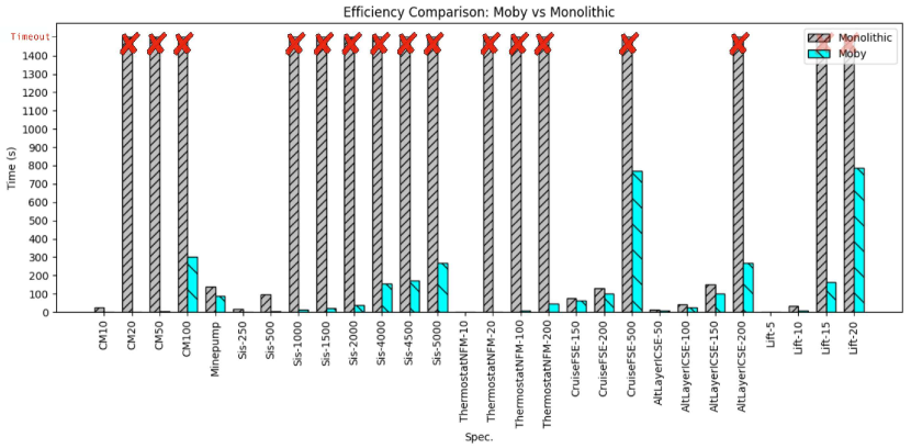
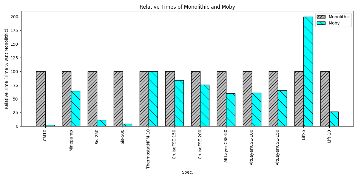
Figure 6: Speed of MoBy vs monolithic synthesis. The figure above shows the time taken by a monolithic synthesis tool and the time taken by MoBy. The figure below normalizes the monolithic time to 100 for those that did not reach Timeout.

To address them, we analyzed specifications from published literature, evaluation of RE tools, and case studies on SCR specification and analysis:

• our counter machine running example CM with varying bounds.

• Minepump: A mine pump controller [7, 9, 15, 41], which manages a pump with sensors that detect high water levels and methane presence.

• Thermostat($n$): A thermostat [22] that monitors a room temperature controls the heater and tracks heating duration.

• Lift($n$): A simple elevator controller for $n$ floors [1].

• Cruise($n$): A cruise control system [35] which is in charge of maintaining the car speed on the occurrence of any event.

• Sis($n$): A safety injection system [16], responsible for partially controlling a nuclear power plant by monitoring water pressure in a cooling subsystem.

• AltLayer($n$): A communicating state machine model [8].

Fig. 4 shows the number of input/output variables, assumptions (A), guarantees (G), and the number of modes for each case.

5.0.1 Experimental Results.

To address RQ1 we compare the size of the original specification with the size of each projection measured by the number of clauses and the formula length. To determine the formula’s length, we adopt the methodologies outlined in [7, 9]. Additionally, we compared the running time required for synthesizing the original specification with the time taken for each projection, note that we report the aggregated time taken to synthesize the systems for each projection, when they can be solved independently and in parallel to potentially improve efficiency. The summarized results can be found in Fig. 5. We also provide additional insights in Fig.6, which highlights the significance of MoBy in enhancing the synthesis time.

Our analysis demonstrates that MoBy successfully decomposes 100% of the specifications in our corpus, which indicates that MoBy is effective in handling complex specifications. Furthermore, MoBy consistently operates within the 25-minute timeout limit in all cases. In contrast, other relevant simultaneous decomposition methods [24, 23] failed to decompose any of the specifications in our benchmark. This can be attributed to the intricate interdependencies between variables in our requirements, as elaborated in Section 1. This observation not only supports the effectiveness of MoBy but also validates RQ2.

Expanding on the impact of MoBy, our results show an average reduction of 64% in specification size and a 65% reduction in the number of clauses. These reductions underscore the advantages of employing MoBy in synthesizing implementations for LTL specifications that are beyond the capabilities of monolithic synthesizers. Additionally, MoBy’s ability to achieve faster synthesis times for feasible specifications positions it as a compelling alternative to state-of-the-art synthesis tools. This suggests the validity of RQ3.

6 Conclusion and Future Work

We presented mode based decomposition for reactive synthesis. As far as we know, this is the first approach that exploits modes to improve synthesis scalability. Our method takes an LTL specification, along with a set of modes representing different stages of execution, and a set of initial conditions for each mode. Our method computes projection for each mode ensuring that if all of them are realizable, then the original specification is also realizable.

We performed an empirical evaluation of an implementation of MoBy on several specifications from the literature. Our evaluation shows that MoBy successfully synthesizes implementations efficiently, including cases for which monolithic synthesis fails. These results indicate that MoBy is effective for decomposing specifications and can be used alongside other decomposition tools.

Even though modes are natural in RE, the need to specify initial conditions is the major drawback of our technique. We are currently investigating how to automatically compute the initial conditions, using SAT based exploration. We are also investigating the assessment of the quality of the specifications generated using MoBy.

References

- [1] The reactive synthesis competition. www.syntcomp.org
- [2] Alur, R., Torre, S.L.: Deterministic generators and games for LTL fragments. In: Proc. of LICS’01. pp. 291–300. ACM (2001)
- [3] Balachander, M., Filiot, E., Raskin, J.F.: LTL reactive synthesis with a few hints. In: Proc. of TACAS’23 (Part II). LNCS, vol. 13993, pp. 309–328. Springer (2023)
- [4] Bansal, S., Li, Y., Tabajara, L.M., Vardi, M.Y.: Hybrid compositional reasoning for reactive synthesis from finite-horizon specifications. In: AAAI’20
- [5] Bharadwaj, R., Heitmeyer, C.: Applying the SCR requirements method to a simple autopilot. In: NASA CONFERENCE PUBLICATION. pp. 87–102. NASA (1997)
- [6] Bloem, R., Jobstmann, B., Piterman, N., Pnueli, A., Sa’ar, Y.: Synthesis of reactive(1) designs. JCSS 78(3), 911–938 (2012)
- [7] Brizzio, M., Cordy, M., Papadakis, M., Sánchez, C., Aguirre, N., Degiovanni, R.: Automated Repair of Unrealisable LTL Specifications Guided by Model Counting. In: Proc. of GECCO’23. pp. 1499––1507. ACM (2023)
- [8] Bultan, T.: Action language: A specification language for model checking reactive systems. In: Proc. of ICSE. pp. 335–344 (2000)
- [9] Carvalho, L., Degiovanni, R., Brizzio, M., Cordy, M., Aguirre, N., Traon, Y.L., Papadakis, M.: ACoRe: Automated Goal-Conflict Resolution. In: Proc. of FASE’23
- [10] Chang, E., Manna, Z., Pnueli, A.: Characterization of temporal property classes. In: Proc. of ICALP’92. LNCS, vol. 623, pp. 472–486. Springer (1992)
- [11] Church, A.: Logic, arithmetic, and automata (1962)
- [12] Church, A.: Application of recursive arithmetic to the problem of circuit synthesis. Journal of Symbolic Logic 28(4) (1963)
- [13] De Giacomo, G., Favorito, M.: Compositional approach to translate LTLf/LDLf into deterministic finite automata. In: Proc. of ICAPS’21. pp. 122–130 (2021)
- [14] De Giacomo, G., Vardi, M.Y.: Linear temporal logic and linear dynamic logic on finite traces. In: Proc. of IJCAI’13. pp. 854––860. AAAI Press (2013)
- [15] Degiovanni, R., Castro, P.F., Arroyo, M., Ruiz, M., Aguirre, N., Frias, M.F.: Goal-conflict likelihood assessment based on model counting. In: ICSE (2018)
- [16] Degiovanni, R., Ponzio, P., Aguirre, N., Frias, M.: Improving lazy abstraction for SCR specifications through constraint relaxation. STVR 28(2), e1657 (2018)
- [17] D’Ippolito, N., Braberman, V.A., Piterman, N., Uchitel, S.: Synthesizing nonanomalous event-based controllers for liveness goals. TOSEM 22(1) (2013)
- [18] Dureja, R., Rozier, K.Y.: More scalable LTL model checking via discovering design-space dependencies . In: Proc. of TACAS’18. pp. 309–327. Springer (2018)
- [19] Ehlers, R., Raman, V.: Slugs: Extensible GR(1) synthesis. In: CAV. Springer (2016)
- [20] Emerson, E.A., Clarke, E.M.: Using branching time temporal logic to synthesize synchronization skeletons. Sci. Comput. Program. 2(3), 241–266 (1982)
- [21] Esparza, J., Křetínskỳ, J.: From LTL to deterministic automata: A safraless compositional approach. In: Proc. of CAV’14. pp. 192–208. Springer (2014)
- [22] Fifarek, A., Wagner, L., Hoffman, J., Rodes, B., Aiello, A., Davis, J.: SpeAR v2.0: Formalized past LTL specification and analysis of requirements. In: NFM (2017)
- [23] Filiot, E., Jin, N., Raskin, J.F.: Compositional algorithms for LTL synthesis. In: Proc. of ATVA. pp. 112–127. Springer (2010)
- [24] Finkbeiner, B., Geier, G., Passing, N.: Specification decomposition for reactive synthesis. ISSE (2022)
- [25] Finucane, C.P., Jing, G., Kress-Gazit, H.: Designing reactive robot controllers with LTLMoP. In: Proc. of AAAIWS’11 (2011)
- [26] Giannakopoulou, D., Mavridou, A., Rhein, J., Pressburger, T., Schumann, J., Nija, S.: Formal requirements elicitation with FRET. In: In REFSQ’20
- [27] Heitmeyer, C.: Requirements models for critical systems. In: Software and Systems Safety, pp. 158–181. IOS Press (2011)
- [28] Heitmeyer, C., Labaw, B., Kiskis, D.: Consistency checking of SCR-style requirements specifications. In: Proc. of RE’95. pp. 56–63. IEEE (1995)
- [29] Heitmeyer, C., Pickett, M., Leonard, E., Archer, M., Ray, I., Aha, D., Trafton, G.: Building high assurance human-centric decision systems. AuSE 22, 159–197 (2015)
- [30] Heitmeyer, C.L., McLean, J.D.: Abstract requirements specification: A new approach and its application. IEEE TSE (5), 580–589 (1983)
- [31] Heninger, K.L.: Software requirements for the a-7e aircraft. NRL Memorandum Report 3876, Naval Research Laboratory (1978)
- [32] Hermo, M., Lucio, P., Sánchez, C.: Tableaux for realizability of safety specifications. In: Proc. of FM’23. pp. 495–513 (2023)
- [33] Iannopollo, A., Tripakis, S., Vincentelli, A.: Specification decomposition for synthesis from libraries of LTL assume/guarantee contracts. In: DATE. IEEE (2018)
- [34] Jacobs, S., Klein, F., Schirmer, S.: A high-level LTL synthesis format: TLSF v1.1. EPTCS 229, 112–132 (11 2016)
- [35] Kirby, J.: Example NRL SCR software requirements for an automobile cruise control and monitoring system. Wang Inst. of Graduate Studies (1987)
- [36] Kress-Gazit, H., Wongpiromsarn, T., Topcu, U.: Correct, reactive, high-level robot control. IEEE Robotics & Automation Magazine 18(3), 65–74 (2011)
- [37] Kretínský, J., Meggendorfer, T., Sickert, S.: Owl: A library for -words, automata, and LTL. In: Proc. of ATVA’18. pp. 543–550. Springer (2018)
- [38] Kupferman, O.: Recent challenges and ideas in temporal synthesis. In: SOFSEM’12
- [39] Kupferman, O., Piterman, N., Vardi, M.Y.: Safraless compositional synthesis. In: Proc. of CAV’06. pp. 31–44. Springer (2006)
- [40] Kupferman, O., Vardi, M.Y.: Model checking of safety properties. Formal Methods in System Design 19, 291–314 (2001)
- [41] Letier, E., Kramer, J., Magee, J., Uchitel, S.: Deriving event-based transition systems from goal-oriented requirements models. AuSE 15, 175–206 (2008)
- [42] Li, J., Pu, G., Zhang, L., Yao, Y., Vardi, M.Y., He, J.: Polsat: A portfolio LTL satisfiability solver (2013), http://arxiv.org/abs/1311.1602
- [43] Mallozzi, P., Incer, I., Nuzzo, P., Sangiovanni-Vincentelli, A.L.: Contract-based specification refinement and repair for mission planning. In: FormaliSE’23
- [44] Manna, Z., Pnueli, A.: Temporal verification of reactive systems: safety. Springer-Verlag, New York, USA (1995). https://doi.org/10.1007/978-1-4612-4222-2
- [45] Mavin, A., Wilkinson, P., Harwood, A., Novak, M.: Easy approach to requirements syntax (EARS). pp. 317 – 322 (10 2009). https://doi.org/10.1109/RE.2009.9
- [46] Meyer, P.J., Sickert, S., Luttenberger, M.: Strix: Explicit reactive synthesis strikes back! In: Proc. of CAV’18 (Part I). pp. 578–586. Springer (2018)
- [47] Pnueli, A.: The temporal logic of programs. In: SFCS’77. pp. 46–57. IEEE (1977)
- [48] Pnueli, A., Rosner, R.: On the synthesis of a reactive module. In: POPL’89
- [49] Pnueli, A., Zaks, A.: PSL model checking and run-time verification via testers. In: Proc. of FM’06. LNCS, vol. 4085, pp. 573–586. Springer-Verlag (2006)
- [50] de Roever, W.P., Langmaack, H., Pnueli, A. (eds.): Compositionality: The Significant Difference. Springer (1998). https://doi.org/10.1007/3-540-49213-5
- [51] van Schouwen, A.J., Parnas, D.L., Madey, J.: Documentation of requirements for computer systems. In: Proc. of ISRE. pp. 198–207. IEEE (1993)
- [52] Sistla, A.P.: Safety, liveness, and fairness in temporal logic. FAC 6, 495–511 (1994)
- [53] Zhu, S., Tabajara, L.M., Li, J., Pu, G., Vardi, M.Y.: A symbolic approach to safety LTL synthesis. In: Proc. of HVC. pp. 147–162. Springer (2017)