CAT: A Causally Graph Attention Network for Trimming Heterophilic Graph

Abstract

Local Attention-guided Message Passing Mechanism (LAMP) adopted in Graph Attention Networks (GATs) is designed to adaptively learn the importance of neighboring nodes for better local aggregation on the graph, which is able to effectively bring the representations of similar neighbors closer, thus shows stronger discrimination ability. However, existing GATs suffer from a significant discrimination ability decline in heterophilic graphs because the high proportion of dissimilar neighbors can weaken the self-attention of the central node, jointly resulting in the central node’s deviation from similar nodes in the representation space. This kind of effect generated by neighboring nodes is referred to as Distraction Effect (DE) in this paper. In order to estimate and weaken the DE of neighboring nodes, we propose a Causally graph Attention network for Trimming heterophilic graph (CAT). To estimate the DE, since the DE are generated through two paths (grab the attention assigned to neighbors and reduce the central node’s self-attention), we use Total Effect to model DE, which is a kind of causal estimand and can be estimated from intervened data; To weaken the DE, we identify the neighbors with the highest DE (we call them Distraction Neighbors) and remove them. We adopt three representative GATs as the base model within the proposed CAT framework, and conduct experiments on seven heterophilic datasets in three different sizes. Comparative experiments show that CAT is able to improve the node classification accuracy of all base GAT models. Ablation experiments and visualization further validate the enhancement of discrimination ability brought by CAT. Besides, the framework of CAT is plug-and-play and can be introduced to any LAMP-driven GATs because it learns a trimmed graph in the attention learning stage, instead of modifying model architecture or searching for new neighbors globally. The source code is available at https://github.com/GeoX-Lab/CAT.

1 Introduction

Graph Neural Network (GNN) is the most reliable and prevailing benchmark model for graph learning. With its effectiveness in representing irregular graph data, GNN achieves state-of-the-art performance in tasks such as node classification, link prediction, graph classification, graph generation and graph similarity calculation [1], and has also been widely applied in recommend system [2, 3, 4, 5, 6], computer vision [7, 8, 9, 10], natural language processing [11], molecular [12, 13, 14, 15], transportation [16, 17, 18, 19], the internet of things [20], epidemiology [21] and other fields. The power of GNN in graph representation primarily stems from its ability to aggregate information, mostly followed the message passing mechanism [22, 23], which can build invariant input representations for the central node based on its local neighbors. Existing GNNs vary in different aggregation operation in accordance with their fundamental assumption about the influence of neighbors, but mostly are built on strong homophily hypothesis of the graph, which obeys the rule that neighbors tend to be similar [24]. Among them Graph Attention Network (GAT) [25] is a representative one, which adaptively learns the importance of neighbors for aggregation through the Local Attention-guided Message Passing Mechanism (LAMP), thereby has the potential for better performance on high homophily graphs. However, the reverse of the coin is a decline when dealing with low homophily graphs. Experiments have shown that GNNs under a strong homophily hypothesis experience significant decline in node classification task [24] when the input graph is heterophilic, and we find that LAMP-driven models like GAT get the most conspicuous decline (as shown in Section 4.1). The main reason is the presence of a high proportion of dissimilar neighbors. Dissimilar neighbors influence the representation of the central node through their assigned attention and weaken the self-attention of the central node, both can result in the central node deviating from its similar nodes in the representation space. We refer to this impact of neighboring nodes on the central node as Distraction Effect (DE), which is generated through two paths (capturing the attention assigned to neighbors and reducing the central node’s self-attention) and leads to the deviation of the representation of central nodes. How to improve the discrimination ability on heterophilic graphs is an important challenge for GATs to overcome.

Existing methods primarily propose solutions for improving the discrimination ability on heterophilic graphs of general GNNs, with only a few offering specific solution for GATs. These approaches can be categorized into two groups: GNN Architecture Tactic and Graph Structure Tactic. GNN Architecture Tactic focuses on modifying the GNN architecture to better utilize the information from neighboring nodes for aggregation. Novel aggregation mechanisms are proposed to adjust the weights of neighbors [26, 27, 28, 29, 30, 31], and some works try to fuse information from different GNN layers in a new way [32, 33, 34, 35]. Self-supervised learning is also adopted to capture more information from neighbors [36, 37, 38]. Graph Structure Tactic, on the other way, focuses on making heterophilic graphs more homophilic by finding more similar nodes for aggregation. These methods tend to look for high-order neighbors [39, 40] or nearest neighbors in some hidden space [41, 42, 43, 44, 45, 46], forcing the central node to be closer to similar nodes in the representation space. Specific methods for GATs adjust the attention coefficient of neighbors by improving the attention mechanism [47, 48], which can be considered as a deduction of GNN Architecture Tactic.

In general, existing methods primarily focus on addressing a singular issue: how to enhance the aggregation of information from other nodes? The GNN Architecture Tactic targets at the Aggregation Mechanism, while the Graph Structure Tactic targets at the Aggregation Object. However, the Aggregation operation is derived from strong homophily hypothesis, which is not satisfied by heterophilic graphs. Therefore, modifying the Aggregation operation is not an essential way. Besides, more similar aggregation objects which can improve the homophilic ratio is not a necessary condition to explain the poor performance on heterophilic graphs of GNNs [24], and has the potential over-smoothing crisis.

Contrary to the emphasis on Aggregation, we propose a new insight with the consideraion of the mechanism of GATs: enabling the central node to concentrate on itself while avoiding the distraction caused by a subset of neighbors can improve the discrimination ability of GATs on heterophilic graphs. We depict a toy example in Figure 1. For heterophilic graphs, the high proportion of inter-class edges lead to the updated representation of the central node deviating from the distribution of its own class, even when similar neighbors are assigned higher weights; Whereas after graph trimming, despite the increased homophilic ratio, the representation of the central node deviates less and is classified correctly due to higher self-attention and lower distraction. Since the removed nodes contribute to the decreased self-attention of the central node, and removing them helps prevent the occurring deviation, we refer to these nodes as Distraction Neighbors. They mathematically equal to the neighbors with High DE on the central node.

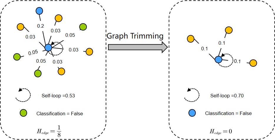
Figure 1: Toy example: The comparison between low self-attention and high self-attention for the central node.

In order to identify and remove Distraction Neighbors, we need to measure the DE of neighboring nodes on the central node, that is, the effect on the attention distribution of the central node generated from its neighbors. Therefore, two crucial questions need to be answered.

Question 1: What is the basic unit of Distraction Neighbors when influencing the attention learning of the central node?

Answer 1: Using two two heterophilic graphs as an example, we intervene the Local Neighbor Distribution (LND) of nodes and design three control groups to explore the effect of LND on the discrimination ability of the central node (Section 4.1). Experiments reveal that the semantic information provided by nodes of the same class is similar, referred to as Class-Level Semantic. Based on this observation, we introduce the concept of Class-Level Semantic Cluster and further propose the Class-Level Semantic Space hypothesis in (Section 4.2). In this hypothesis, we believe that neighbors of the same class have the similar impact on identifying the central node, therefore the basic unit for measuring DE should be class. It is more beneficial to get the genuine and stable effect of neighbors by treating the neighbors of the same class as a group.

Module 1. Based on Answer 1, we design the Class-level Semantic Clustering Module, to pre-cluster local neighbors and get different Semantic Clusters for measuring their DE on the central node.

Question 2: How much the Distraction Neighbors has impacted the attention learning of the central node?

Answer 2: To better estimate the DE, we model DE as a type of causal effect. Specially, we formalize the influencing paths of neighboring nodes on the central node’s attention learning based on the working mechanism of GATs and construct a causal graph (Figure 2 and Figure 9). A causal graph is a graphical language capable of measuring causal effects through the manipulation of causal variables, referred to as intervention. Since the neighboring nodes influence the central node through two paths, we chose the Total Effect to estimate the overall causal effect.

Module2. Based on Answer 2, we design the Total Effect Estimation Module, Intervene the LND of central node with Semantic Cluster as the basic unit, then calculate the TE from the changes of the central node’s attention distribution before and after intervention. Distraction Neighbors are identified and removed in accordance with TE and the corresponding trimmed graph are generated.

Our contributions are as follows:

1. We propose a novel insight to enhance GAT’s discrimination ability on heterophilic graphs: maintaining the central node’s self-attention while avoiding distraction caused by neighbors. Instead of altering the architecture of GAT and searching for new neighbors globally, we use the attention distributed learned by GAT as signal to identify and remove Distraction Neighbors, which can be regarded as a trimming operation on the graph.

2. We propose a Causally graph Attention network for Trimming heterophilic graph (CAT) to improve the discrimination ability of GAT on heterophilic graphs. We employed three GATs as base model and conducted node classification experiments on seven datasets in three different sizes. Comparison Experiments show all base model can perform better within the CAT architecture. Ablation experiments and visualization experiments further validate the effectiveness.

3. We conduct pre-experiments and analyze the mechanism that how LND influence the attention learning of the central node based on our observations and background knowledge. We further formalize it into a causal graph where the causal effect of neighbors can be estimated with manipulations.

The rest of this paper is mainly organized as follows: in Section 2, we classify and summarize the existing methods on heterophilic graphs for both generous GNN and GAT-oriented, and list the differences between our methods and theirs. In Section 3, we introduce some important concepts and background knowledge needed for this paper, including the causal graphs derived from the background knowledge; In Section 4, we present the pre-experiments we did and the hypotheses we drew from the experiment results. We introduce our method in Section 5 and describe the dataset and experiments in Section 6. In Section 7 and Section 8, we discuss and conclude the work, fundamental issues that are inspiring and need to be answered in the future are also proposed.

2 Related Work

Strong homophily underlying graphs hypothesizes that connected nodes are similar, which is a necessity of GNNs. This principle is also widely acknowledged in various domains such as social networks [49] and citation networks [50, 51, 52]. Under this assumption, aggregating the information of neighbors gradually brings nodes of the same class closer in the representation space, thereby improving the discrimination ability of GNNs. However, when confronted with heterophilic graphs, the merit of GNNs may turn into a nightmare. The decline of GAT is especially obvious (Section 4.1). GNNs for heterophilic graphs have attracted increasing attention, and how to improve their discrimination ability poses significant challenges. A growing body of research has been developed to overcome the heterophilic challenges, and we categorized them into two groups based on their fundamental strategies: GNN Architecture Tactic and Graph Structure Tactic.

GNN Architecture Tactic. This kind of approach achieves better learning and fusion of neighbors’ information by altering the architecture of GNN.

1. Some methods aim to modify the aggregation operation in message passing. Ordered GNN [30] leverages a rooted-tree hierarchy aligning strategy to order the message passing, thereby achieving better fusion of information provided by nodes in different hops. NHGCN [29] designs a new metric, Neighborhood Homophily (NH) to group and aggregate the neighbors differently. LW-GCN [28] proposes a label-wise message passing mechanism that use pseudo labels to guide the aggregation of similar nodes and preserve the heterophilic contexts. DMP [26] takes the attributes as weak labels to measure attribute homophily rate, which can specify the attribute weight of edges for aggregation. CPGNN [27] incorporates an interpretable compatibility matrix for modeling the heterophily or homophily level, and uses the matrix to propagate and update the prior belief of each nodes. GGCN [31] proposes two strategies, structure-based and feature-based edge correction to adjust edges weights for aggregation.

2. Some methods aim to design different GNN layers and their relationships. Auto-HeG [33] builds a comprehensive GNN search space from which the optimal heterophilic GNN is selected. IIE-GNN [35] designs a GNN framework that contains seven blocks in four layers to enrich the intra-class information extraction. H2GCN [34] uses a combination of intermediate layers to concatenate the node representations from all previous layers, so as to capture local and global information better. GPR-GNN [32] combins a Generalized PageRank with GNN to learn weights of GNN layers for combination of intermediate layer representation.

3. Some methods aim to train GNNs in a new learning paradigm. HLCL [36] uses graph filters to generate augmented graph views and contrast the high-pass filter representation with the low-pass part for graph contrastive learning under heterophily. MVGE [37] builds two augmentation views with the input of ego features and aggregated features respectively, and forces the model to learn different graph signal through graph reconstruction task. SimP-GCN [38] employes self-supervised learning to capture the complex feature similarity and dissimilarity relations between nodes, which can help conduct the node similarity preserving aggregation.

Graph Structure Tactic. This kind of approach primarily involves modifying the connectivity of the graph, restructuring the graph by searching for more similar neighbors, and aggregating their information.

1. Some methods seek for similar neighbors from high-order neighbors. U-GCN [40] uses a multi-type convolution mechanism to capture and fuse the information from 1-hop, 2-hop and kNN neighbors. GPNN [39] adds the most relevant nodes from a large amount of multi-hop neighborhoods, and filters out irrelevant or noisy nodes from local neighborhoods.

2. Some methods search for nearest neighbors in a learned feature space. GEOM-GCN [42] learns a latent space and aggregate information from neighbors in latent space to strengthen the GCN’s ability to capture long-range dependencies in heterophilic graphs. Non-local GNNs [44] leverages attention mechanism to sort and find distant but informative nodes for conducting non-local aggregation. HOG-GCN [45] designs a novel propagation mechanism guided by the homophily degree between node pairs learned in the homophily degree matrix estimation module, to explore more similar node pairs. GCN-SL [41] uses spectral clustering to construct a re-connected graph according to the similarities between nodes and perform aggregation on the re-connected graph. A graph restructuring method [46] based on adaptive spectral clustering improves the node classification accuracy of GNN by improving graph homophily. DHGR [43] rewires graph by adding homophilic edges and pruning heterophilic edges, and the similarity of label/feature-distribution of node neighbors is adopted to determine the rewiring.

There are also researches focused on solutions for GATs, we called them GAT-oriented methods. HA-GAT [48] proposes a heterophily-aware attention scheme to assign weights for edges adaptively, and learns the local attention pattern of the central node by learning importance of each heterophilic edge type to get the final attention coefficient. GATv3 [47] proposes a new attention architecture to compute the attention coefficients between query and key, which improves the quality of the representations of nodes connected by heterophilic edges by introducing the representations learned by other GNNs. This type of approaches belongs to GNN Architecture Tactic.

Difference to GNNs for heterophilic graph. Our approach differs from the above GNNs for heterophilic graph in that it does not require altering the original GAT model or searching for new neighbors globally in the graph, but instead removes Distraction Neighbors in a graph trimming manner. It enables GAT to fully utilize its attention mechanism to improve its discrimination ability on heterophilic graphs.

Difference to GAT-oriented methods. Our approach is different from the above approaches targeted at GAT in that we do not need to change the attention mechanism of the original GAT model; instead, we make full use of the learned attention distribution of the original GAT model as a signal to find a better attention distribution. Therefore, our method is plug-and-play and applicable to any LAMP-driven GATs.

3 Preliminaries

Semi-supervised Graph Node Classification. Graph node classification is a fundamental task in graph representation learning, with the purpose of classifying graph nodes into predefined categories [53], and can be used as a proxy task for measuring the discrimination ability of graph representation models. Existing methods mainly focus on Semi-supervised paradigm. Given a graph $G=(V,E)$, where $V$ is the set of nodes and $E$ is the set of edges. $A\in\mathbb{R}^{N\times N}$ is the adjacency matrix of the graph, $X\in\mathbb{R}^{N\times F}$ is the node feature matrix. The number of layers of the GNN model is $K$, the node representation in layer $k\in\{1,2,\ldots K\}$ is $z^{k}\in\mathbb{R}^{N\times H}$, where $H$ denotes the representation dimension in hidden layer. In this task, each node belongs to a specific category, only the labels of nodes in the training set are visible, and the target is to predict the category of nodes unlabeled.

Graph Attention Network. GAT is a graph neural network architecture that can adaptively learn the importance of neighboring nodes by leveraging attention mechanism to get the weights of neighbors [25]. The graph attention layer depicts how to get the representation $z^{k}\in\mathbb{R}^{N\times H_{k}}$ in layer $k$ with the input of representation $z^{k-1}\in\mathbb{R}^{N\times H_{k-1}}$ in layer $k-1$. The attention coefficient $\alpha_{ij}$ between a pair of nodes $(i,j)$ where $A_{ij}\neq 0$ is calculated by a linear transformation layer $W\in\mathbb{R}^{H_{k-1}\times H_{k}}$ and a shared attention mechanism $a:\mathbb{R}^{H_{k-1}}\times\mathbb{R}^{H_{k}}\rightarrow\mathbb{R}$ according to Eq.1.

$$\alpha_{ij}=\frac{\exp\left(\sigma\left(W_{2}\left[WZ_{i}^{k-1}||WZ_{j}^{k-1}\right]\right)\right)}{\sum_{m\in N(i)}\exp\left(\sigma\left(W_{2}\left[WZ_{i}^{k-1}||WZ_{m}^{k-1}\right]\right)\right)}$$ (1)

Let $H_{i}^{k}=\sigma\left(\sum_{j\in N(i)}\alpha_{ij}WZ_{j}^{k-1}\right)$ denote the updated representation of the central node $V_{i}$. Where $W_{2}\in\mathbb{R}^{1\times 2H^{k}}$ is a linear transformation layer, $\sigma(\cdot)$ is a nonlinear activation function, $\|$ represents the concatenation operation. If multi-head attention mechanism is applied, the node representation will be calculated for each attention head, and the final representation will be calculated with all attention heads according to Eq.2.

$$H_{i}^{k}=\Delta_{t=1}^{T}H_{i}^{k}$$ (2)

Where $\Delta(\cdot)$ stands for concatenation, average or other pooling operations.

Causal Inference. Causal inference is a new science for data [54], by making causal claims rather than merely associational claims with the belief that causality is inherently more stable. It is concerned with (1) Causal Discovery: Is there causal relationship between two variables? How does the cause impact the effect? And (2) Causal Effect Estimation: How much does the cause impact the effect? There are several important notations used in this paper.

• Cause and Effect. A variable $X$ is said to be a cause of a variable $Y$ if $Y$ can change in response to changes in $X$. Or we can say $Y$ is ‘Listen to’ $X$. Then $X$ is the Cause and $Y$ is the Effect. If $Y$ directly responds to $X$, then $X$ is the Direct Cause of $Y$.

• Causal Graph. A causal graph is a Directed Acycling Graph (DAG) that model the causality with graphical language. In Causal Graphs, every parent is a Direct Cause of all its children.

• Intervention. If we do intervention in a variable $Z$ in the causal graph, it deletes all the edges from the parent variables and set the intervened variable to $\bar{z}$. We can denote it as the operation $do(Z=\bar{z})$. The children of $Z$ would change naturally with the change of $Z$.

• Total Effect (TE). Total Effect measures the whole effect on $Y$ caused by $X$, including the direct effect and indirect effect. The TE can be counted by $TE_{x\rightarrow\bar{x}}=Y(X=x)-Y(do(X=\bar{x}))$.

With the Preliminaries we proposed above, we can depict the causal graph underlying GAT in accordance with Eq.1 and Eq.2, as shown in Figure 2.

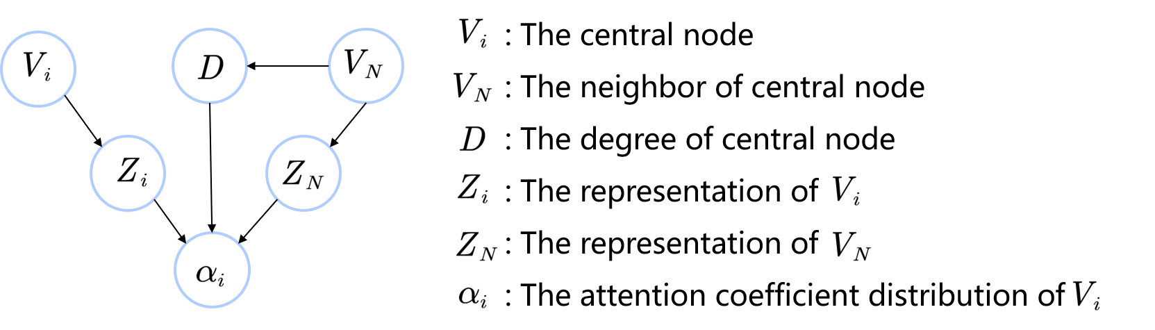
Figure 2: Causal graph behind GAT.

• $V_{i}\rightarrow Z_{i}\rightarrow\alpha_{i}\leftarrow Z_{N}\leftarrow V_{N}$: The attention coefficient distribution of the central node $V_{i}$ is calculated from the representation of $V_{i}$ and $V_{N}$.

• $V_{N}\rightarrow D\rightarrow\alpha_{i}$: When the normalization of attention coefficients is applied, the neighboring nodes will influence the attention distribution of the central node through the degree of the central node.

It is not difficult to notice that $V_{N}$ affects the final attention distribution $\alpha_{i}$ of $V_{i}$ through two causal paths. On the one hand, the representation of the $V_{N}$ itself affects its importance to $V_{i}$. On the other hand, the degree of $V_{i}$ changes due to the existence of $V_{j}\in V_{N}$, and thus affects the final attention coefficients distribution when normalizing $\alpha$. In order to measure the effect of one (or more) neighboring node(s) on the central node’s learned attention, we choose TE to carry out the calculation on causal effect of neighboring nodes, which can be adopted as a measurement of their DE.

We estimate the TE by intervening the LND of $V_{i}$. As illustrated in Figure 3, for a neighboring node $V_{j}\in V_{N}$, $V_{j}=0$ represents the reservation of $V_{j}$ as a neighbor of $V_{i}$, while $V_{j}=1$ represents removing $V_{j}$ from $V_{N}$. According to the Eq.3, we can display how to estimate the effect on the attention coefficient distribution of $V_{i}$ caused by $V_{j}$.

$$TE_{\alpha_{i}}=E_{\alpha_{i}\mid do\left(V_{j}=1\right)}\left[\alpha_{i}\mid\operatorname{do}\left(V_{j}=1\right)\right]-E_{\alpha_{i}\mid do\left(V_{j}=0\right)}\left[\alpha_{i}\mid\operatorname{do}\left(V_{j}=0\right)\right]$$ (3)

Similarly, we denote the self-attention coefficient that $V_{j}$ assigns to itself as $\alpha_{self\_attention}$, and we can get the TE of $V_{j}$ for the self-attention of $V_{i}$ according to Eq.4:

$$\begin{split}TE_{\alpha_{self\_attention}}&=E_{\alpha_{self\_attention}\mid do\left(V_{j}=1\right)}\left[\alpha_{self\_attention}\mid\operatorname{do}\left(V_{j}=1\right)\right]\\ &-E_{\alpha_{self\_attention}\mid do\left(V_{j}=0\right)}\left[\alpha_{self\_attention}\mid\operatorname{do}\left(V_{j}=0\right)\right]\end{split}$$ (4)

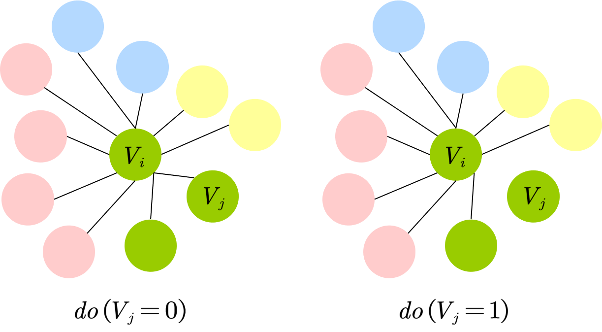
Figure 3: Intervention on the local neighbor distribution of the central node.

4 Pre-experiments and Key Hypothesis

In this section, we depict our observation from designed pre-experiments in Section 4.1 and key hypothesis in Section 4.2. In the pre-experiments, we disentangle the effect of neighboring nodes into two factors and manipulate them to generate intervened graphs as treatment groups. The experiment results indicate that nodes in the same class can provide similar semantic information for discrimination, where Class-level Semantic Space Hypothesis can be derived. We also propose the inference of Class-level Semantic Space Hypothesis, Low Distraction and High Self-attention, which is the core strategy of our method.

4.1 The Effect of Local Neighbor Distribution(LND)

The most important characteristic of GNN is the ability to aggregate the information provided by neighboring nodes and update the representation of the central node, therefore, the Local Neighbor Distribution (LND) is an important contributing factor on the ability of GNN models. As illustrated in Figure 4a, LND can be decomposed into two factors, Class-wise and Degree. The former statistically characterizes the distribution of neighboring nodes in different classes, and the latter denotes the number of neighboring nodes. Figure 4b illustrates that different Class-wise will change the local homophily of central node, and Figure 4c illustrates that LND with same homophily would be significantly different under different Degree. We formalize the LND of nodes in graph $G$ as $LND_{G}=\left\{W_{c},D_{c}\right\},c\in C$, where $C$ denotes the set of classes of nodes in $G$.

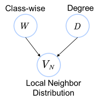
(a)

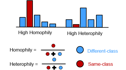
(b)

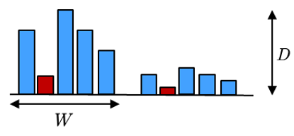
(c)

Figure 4: Local Neighbor Distribution (LND). (a) The two factors that influence LND. (b) How Class-wise influences the LND and the homophily of graph. (c) How Degree influences the LND.

To further discover the influence of LND on discrimination ability of GNN models, we set the graph $G$ as control group and intervene the LND of $G$ to get different treatment groups, for control experiments set up. Then we conduct control experiments on three representative GNN models, GCN [55], GraphSAGE [56] and GAT [25], and compare their node classification accuracy (the outcome of treatment, which is represented as $Y$) on different groups. The experiment setting is illustrated as Figure 5 and Table 1. We choose two heterophilic graph dataset, Chameleon and Squirrel to conduct the pre-experiment. The setting of experiments groups is as follwing:

1. Control group: original graph $G$.

2. Treatment group 1: reduce the Degree of the central node, and keep the Class-wise constant.

3. Treatment group 2: reduce the Degree of the central node, and set the Class-wise randomly. We set three random groups with the random seed 0, 10, 100.

4. Treatment group 3: the Degree of the central nodes remains constant, while randomly replace the neighboring nodes with different nodes of same class. We search the nodes to replace with the random seed 0, 10, 100.

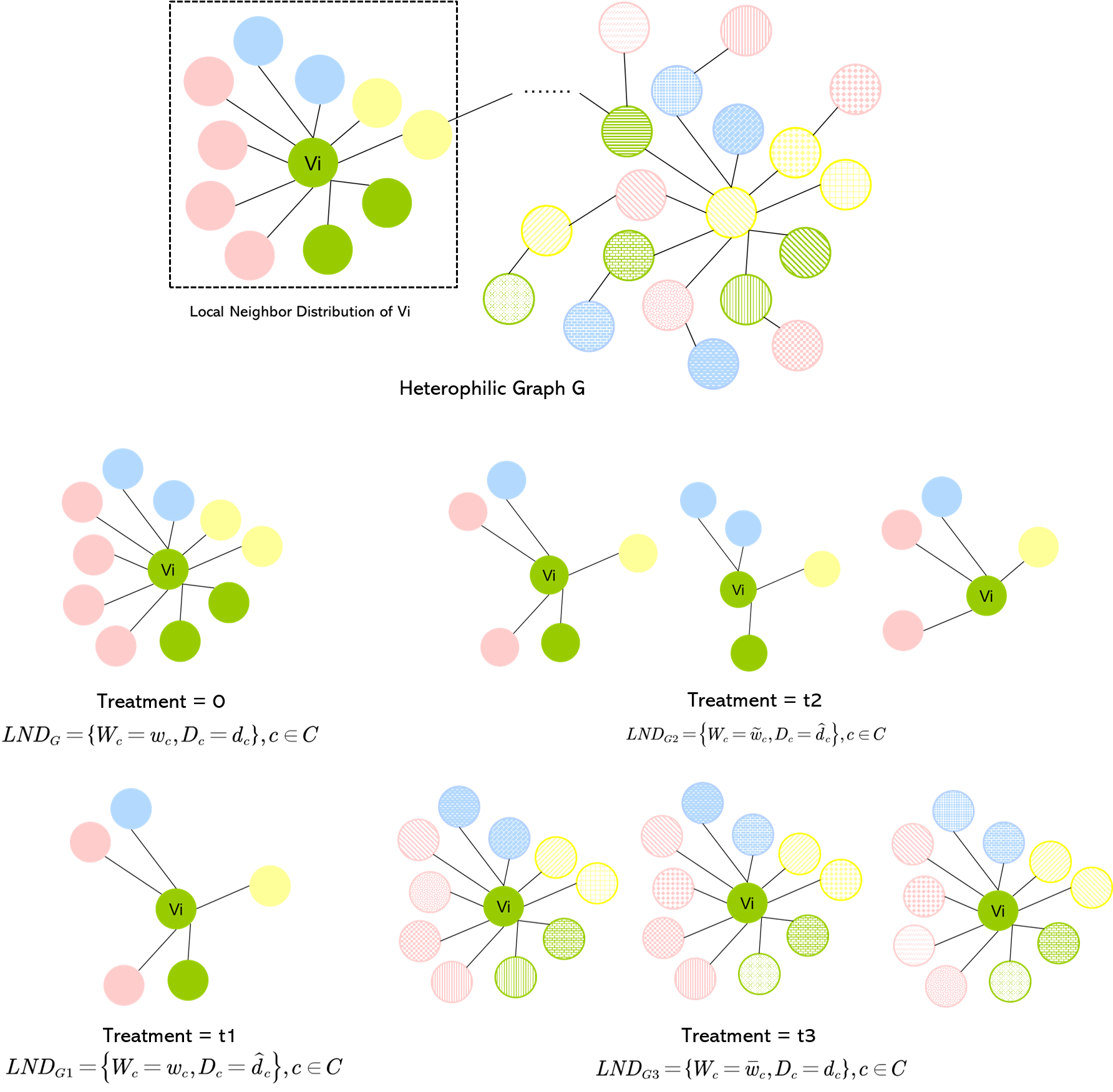
Figure 5: The control and treatment group setting in the pre-experiment.

Table 1: Control experiment setting

Graph/Group	LND
$G$ /treatment=0	$LND_{G}=\left\{W_{c}=w_{c},D_{c}=d_{c}\right\},c\in C$
$G_{1}$ /treatment=$t_{1}$	$LND_{G1}=\left\{W_{c}=w_{c},D_{c}=\hat{d}_{c}\right\},c\in C$
$G_{2}$ /treatment=$t_{2}$	$LND_{G2}=\left\{W_{c}=\widetilde{w}_{c},D_{c}=\widehat{d}_{c}\right\},c\in C$
$G_{3}$ /treatment=$t_{3}$	$LND_{G3}=\left\{W_{c}=\bar{w}_{c},D_{c}=d_{c}\right\},c\in C$

The result of control experiments are illustrated in Figure 6. It can be noted that:

1. $Y\left(t_{0}\right)\approx Y\left(t_{3}\right)$. It indicates that connections between different classes are substitutable, and keeping both $W$ and $D$ constant, but changing the nodes specifically connected in LND has little effect on the discrimination ability. It also indirectly indicates that nodes in the same class provide similar semantic information. We refer to this type of semantic information as Class-Level Semantic.

2. $Y\left(t_{1}\right)\approx Y\left(t_{2}\right)>Y\left(t_{0}\right)$. After removing a portion of the neighbors while keeping $W$ constant, it is instead able to improve the discrimination of graph nodes; while the improvement can be achieved by reducing $D$ and randomly alter $W$, which indicates that a number of connections in the graph are meaningless, and the distribution of such meaningless connecting edges does not present a difference in different classes.

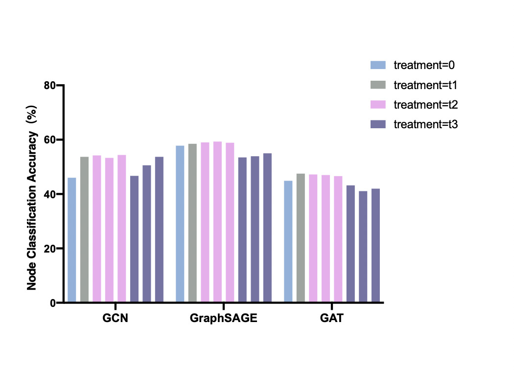
(a) Chameleon

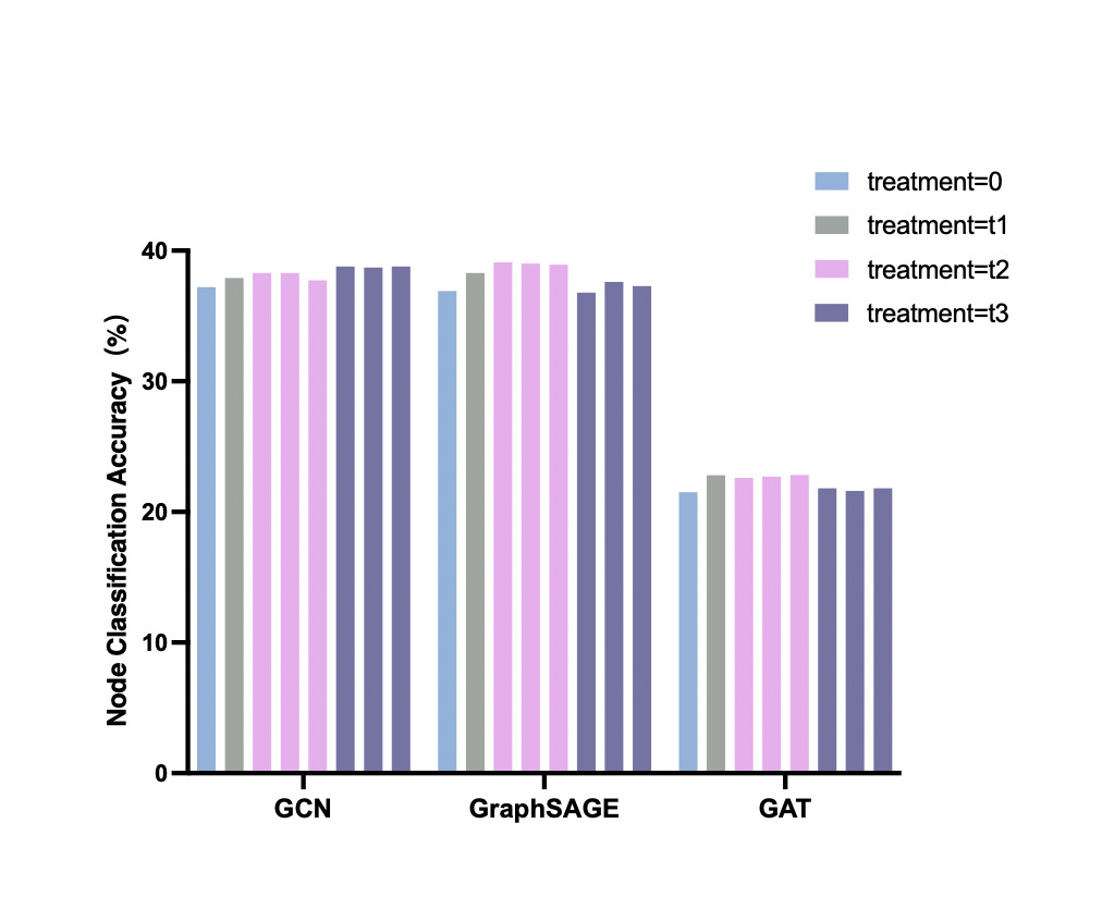
(b) Squirrel

Figure 6: The result of the control experiments.

4.2 Low Distraction and High Self-attention

Drawing on the observations from pre-experiments, we propose a hypothesis and its inference. As illustrated in Figure 7, for a highly heterophilic graph $G$ with nodes of three different classes, the ideal underlying semantic space is comprised of three compact clusters, and each cluster is composed of the mapped graph nodes belong to this class. Each cluster has different size, density and location, and can be distinguished easily from each other. When we observe more nodes of each class, we can obtain a more accurate distribution and shape of its Semantic Clusters. Using a limit-thinking approach, if we could obtain all nodes of a certain class, the Semantic Cluster observed could represent the distribution of all nodes of that class in the semantic space. We refer to this as a Class-level Semantic Cluster, and the ideal space is referred to as Class-level Semantic Space.

Figure 7: An example portrait of ideal semantic space (dimension = 3). The circle with different color represents the distribution of Class-level Semantic Cluster of different class, and the quadrilateral star represents the center of each Class-level Semantic Cluster.

Hypothesis 1: Class-level Semantic Space Hypothesis. The graph $G$ is able to be mapped to an ideal $d$-dimension semantic space $S=f(G)$ , in which nodes of the same class situate very closely and nodes of different classes are as far away from each other as possible. Since an ideal Semantic Cluster is compact, the cluster center can serve as a representation of the distribution of nodes of that class in the semantic space. Therefore, the connections between different classes are substitutable, where each Semantic Cluster center is denoted as Eq.5:

$$s_{c}=\left\{\frac{\sum\limits_{v\in c}s_{v_{1}}}{n_{c}},\frac{\sum\limits_{v\in c}s_{v_{2}}}{n_{c}},\ldots\frac{\sum\limits_{v\in c}s_{v_{d}}}{n_{c}}\right\},c\in C,$$ (5)

$$\text{ s.t. }\sum\limits_{v\in c}\left|s_{v}-s_{c}\right|\rightarrow 0,\frac{1}{\left|s_{c}-s_{j}\right|}\rightarrow 0,j\in\complement_{c}C$$

In the Class-level Semantic Space, it is evident that the closer the central node is to its Semantic Cluster center, the stronger its discrimination ability will be. Since the message passing mechanism aggregates features from neighboring nodes to the central node, neighbors from different classes exert a force that tends to push the central node away from its own Semantic Cluster center, which can be seen as a distraction and should be minimized. Conversely, both neighbors from the same class and the self-attention generate a force that pulls the central node closer to its own Semantic Cluster center, which should be reinforced. In a highly heterophilic graph where neighbors from the same class are rare, it is essential to enhance self-attention while mitigating distraction.

Inference 1: Low Distraction and High Self-attention. For nodes in a heterophilic graph, when nodes make more use of their own information and ignoring information from nodes of different classes while aggregating information, their final representation will be closer to the Semantic Cluster center of their classes in $S$.

Proof. For the central node $v_{i}$ and its neighboring node $v_{j}$, let the aggregation weight be $w$, we can get the representation of $v_{i}$ after aggregation and updating as $h_{i}=\sigma\left(w_{i}\cdot z_{i}+\sum\limits_{j\in N_{i}}w_{j}\cdot z_{j}\right)$, where $h_{i}$ is closer to $s_{ci}$, model’s discrimination ability on $v_{i}$ will be stronger. When the graph is highly heterophilic, $h_{i}$ can be represented as Eq.6:

$$\begin{gathered}w_{i}\cdot z_{i}+\sum\limits_{j\in N_{i}}w_{j}\cdot z_{i}=w_{i}\cdot z_{i}+\sum\limits_{m\in j,v_{m}\in c_{i}}w_{m}\cdot z_{m}+\sum\limits_{n\in j,v_{n}\notin c_{i}}w_{n}\cdot z_{n}\\ \rightarrow w_{i}\cdot s_{c}+\sum\limits_{m}w_{m}\cdot s_{c}+\sum\limits_{n}w_{n}\cdot z_{n}\\ \rightarrow\left(w_{i}+\sum_{m}w_{m}\right)\cdot s_{c}+\sum\limits_{n}w_{n}\cdot z_{n}\\ \text{ s.t. }m\leqslant n;w_{i}+\sum\limits_{m}w_{m}+\sum\limits_{n}w_{n}=1\end{gathered}$$ (6)

Because we hope $h_{i}$ is closer to $s_{ci}$, the optimization object is $\max\left(w_{i}+\sum\limits_{m}w_{m}-\sum\limits_{n}w_{n}\right)$. For the sake of condition in heterophilic graphs that $m\leq n$, we hope the weight for the central node itself $w_{i}$ can be maximized, equals to enhancing the self-attention and avoiding the distraction of dissimilar neighbors.

GAT, functioning as an implicit graph neural network architecture [57], is able to adaptively learn the weights of nodes for guiding the aggregation process. On the one hand, it may be easier to pose the distraction crisis to the central node due to the high proportion of inter-class edges on the heterophilic graph. On the other hand, by learning the weight distribution with Low distraction and High Self-attention, GAT can directly enhance its discrimination ability. Therefore, we foster strengths and circumvent weakness for GAT, leveraging the learned attention distribution as signal to guide the GAT identify and remove the Distraction Neighbors. The operation of graph trimming doesn’t require architecture alternation or new neighbors searching, but learns an optimal attention distribution by enhancing the self-attention.

5 Methodology

5.1 The Architecture of CAT

The Causally graph Attention network for Trimming heterophilic graph (CAT) proposed in this paper mainly contains two important modules: Class-level Semantic Clustering Module and Total Effect Estimation Module. The former obtains the basic unit to estimate TE of neighboring nodes on central node’s attention learning, and the latter further estimates the TE by graph intervention. We introduced the CAT in Algorthim 1, where the $\Theta_{W}$ and $\Theta_{W2}$ of GAT represents the model parameters for learning feature transformation and attention distribution respectively. The pipeline of CAT is illustrated in Figure 8. As illustrated in Figure 8, the framework of CAT can adopt different GATs as the base model, and implement two modules to obtained the trimmed graph that can optimize the attention distribution of the base GAT.

1. Class-level Semantic Clustering Module. This module is derived from the Class-level Semantic Space Hypothesis, which maps the LND of the central node to a space that can discriminate class-level semantic better. The Semantic Clusters output in this module further serve as the basic object for estimating TE on the central node.

2. Total Effect Estimation Module. This module is derived from the Low distraction and High Self-attention, which obtains the TE of each class on the central node by the intervention of different Semantic Clusters. The Distraction Neighbors are identified in accordance with the TE and removed to get the final trimmed graph.

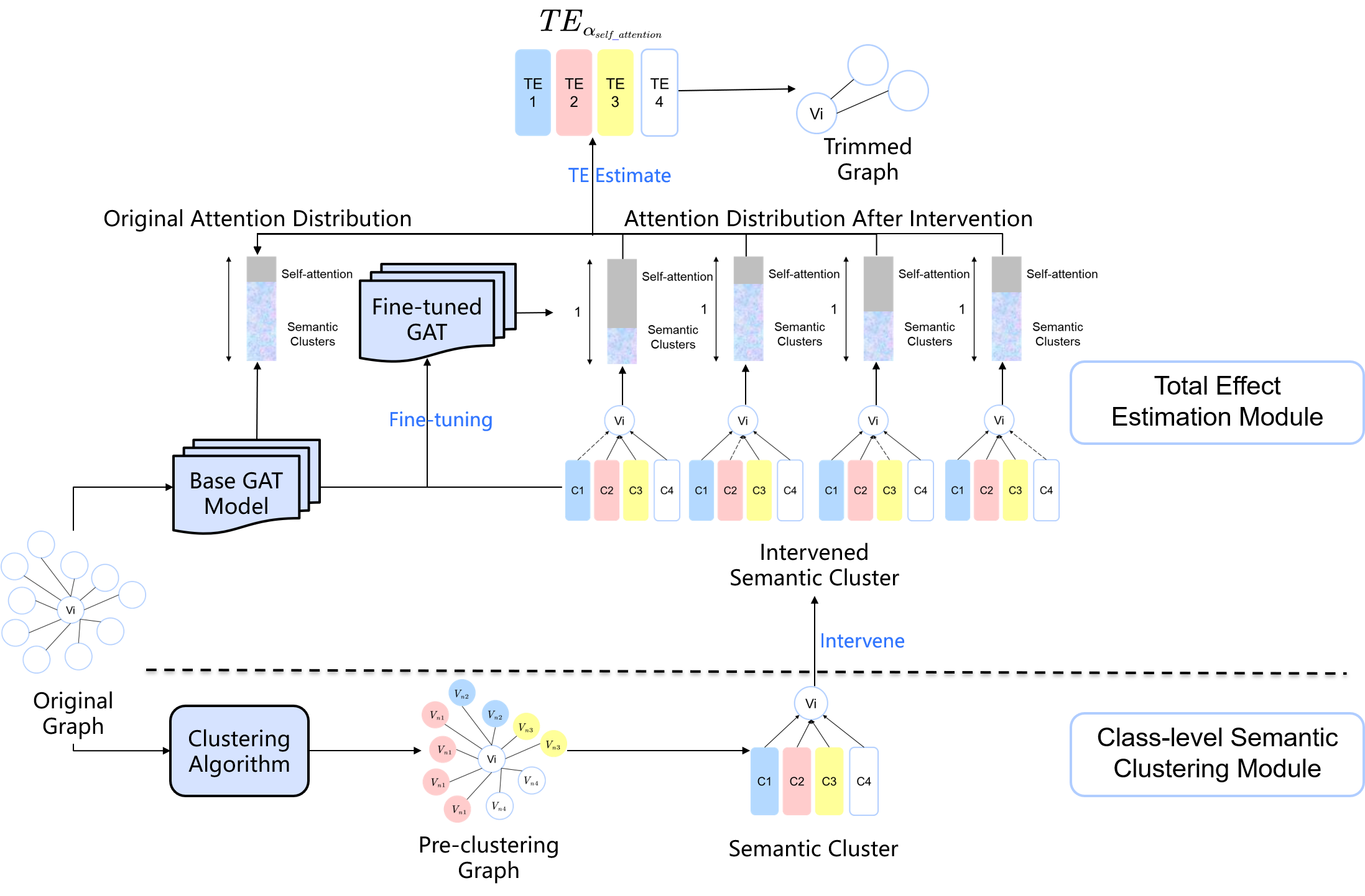
Figure 8: The pipeline of CAT.

input : $G=(V,E)$, $A\in\mathbb{R}^{N\times N}$, $X\in\mathbb{R}^{N\times F}$, $C$, $epoch_{pretrain}$, $epoch_{finetuning}$, $f_{clustering}$, initialized $\Theta_{W},\Theta_{W2}$ of $f_{GAT}$

output : $A_{Trim}\in\mathbb{R}^{N\times N}$

1 // Class-level Semantic Clustering ;

2 $SC=f_{\text{clustering}}(X)$, $SC\in\mathbb{R}^{n\times 1}$;

3 // Pretrain the base GAT ;

4 for $epoch$ in $epoch_{pretrain}$ do

5      $Z,\alpha_{SC},\alpha_{self\_attention}=f_{\text{GAT}}(A,X)$;

6       Update $\Theta_{W},\Theta_{W2}$ of $f_{GAT}$;

7 end for

8Freeze $\Theta_{W}$ and re-initialize $\Theta_{W2}$;

9 // Semantic Cluster intervention ;

10 for $c$ in $C$ do

11       for $V_{i}$ in $V$ do

12             if $A_{ij}=1$ and SC(j)=c then

13                   $\hat{A}_{ij}^{c}=0$ ;

14                  

15             end if

16            

17       end for

18      // Intervened attention learning ;

19       for $epoch$ in $epoch_{finetuning}$ do

20             $Z^{c},\alpha_{SC}^{c},\alpha_{self\_attention}^{c}=f_{\text{GAT}}(\hat{A}^{c},X)$;

21             Update $\Theta_{W2}\longrightarrow f_{GAT}^{c}$;

22            

23       end for

24      

25 end for

26// Graph trimming ;

27 for $c$ in $C$ do

28      $TE_{\alpha_{self\_attention}}^{c}=\alpha_{self\_attention}^{c}-\alpha_{self\_attention}$;

29      

30 end for

31for $V_{i}$ in $V$ do

32       if $A_{ij}=1$ and $SC(j)=\min\left(TE_{\alpha_{self\_attention}}\right)$ then

33             $A_{ij}^{Trim}=1$ ;

34       end if

35      

36 end for

Algorithm 1 Causally graph Attention network for Trimming heterophilic graph(CAT)

5.2 Class-level Semantic Clustering Module

Based on the Class-level Semantic Space Hypothesis, we consider that for the central node, the neighbors impact the self-attention learning with their class as the basic unit. It is very intuitive on heterophilic graphs, when the representations of graph nodes are hard to distinguish, the more nodes we observe for a class, the more beneficial it is to get the global distribution of that class.

In that semantic space, we treat the local neighbors of same cluster as a whole, which is referred to as Semantic Cluster $SC=f_{\text{clustering }}(x),\quad x\in\mathbb{R}^{n\times F},\quad SC\in\mathbb{R}^{n\times 1}$. Where $SC(i)\in C$ represents the cluster class of nodes with the index $i$. Accordantly, the center of each SC in that semantic space is $SC_{c}=\left\{\frac{\sum\limits_{SC(v)=c}SC_{v_{1}}}{n_{c}},\frac{\sum\limits_{SC(v)=c}SC_{v_{2}}}{n_{c}},\ldots\frac{\sum\limits_{SC(v)=c}SC_{v_{d}}}{n_{c}}\right\},c\in C$. We can update the causal graph proposed in Figure 2 to Figure 9.

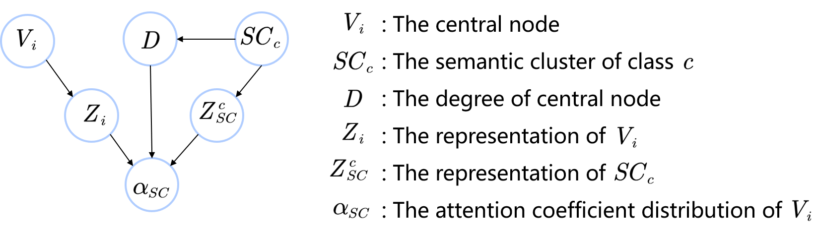
Figure 9: Causal graph behind GAT at the level of Semantic Cluster.

As shown in Figure 10, three learning paradigms can be adopted in this module to obtain Class-level Semantic Clusters, ordered from low to high prior knowledge of the node category distribution they are: unsupervised, semi-supervised, and supervised learning. The more information we acquire about the categorical distribution of graph node, the closer the Semantic Cluster distribution we obtained will be to the distribution in the ideal semantic space. This further indicates a more accurate estimation of the Total Effect of attention learning on Class-level Semantic Cluster corresponding to each category. We construct three CAT variants by adopting following three learning paradigms in this module:

• Unsupervised manner: For all nodes in the graph, their categorical labels are unseen. Unsupervised clustering methods can be employed to obtain a rough semantic space with the input of node features. The CAT variant under this manner is referred to as CAT-unsup.

• Semi-supervised manner: Categorical labels for a fixed ratio of nodes are known and used to inference the labels of unknown nodes. Classification methods with a semi-supervised setting can be employed to obtain a fewer rough semantic space with the input of node features. The CAT variant under this manner is referred to as CAT-semi.

• Supervised manner: Categorical labels for all nodes are known and their categorical distribution is completely and accurately observed. It should be noted that the label information is only available in the Class-level Semantic Clustering stage and will not be used for node classification. The CAT variant under this manner is referred to as CAT-sup.

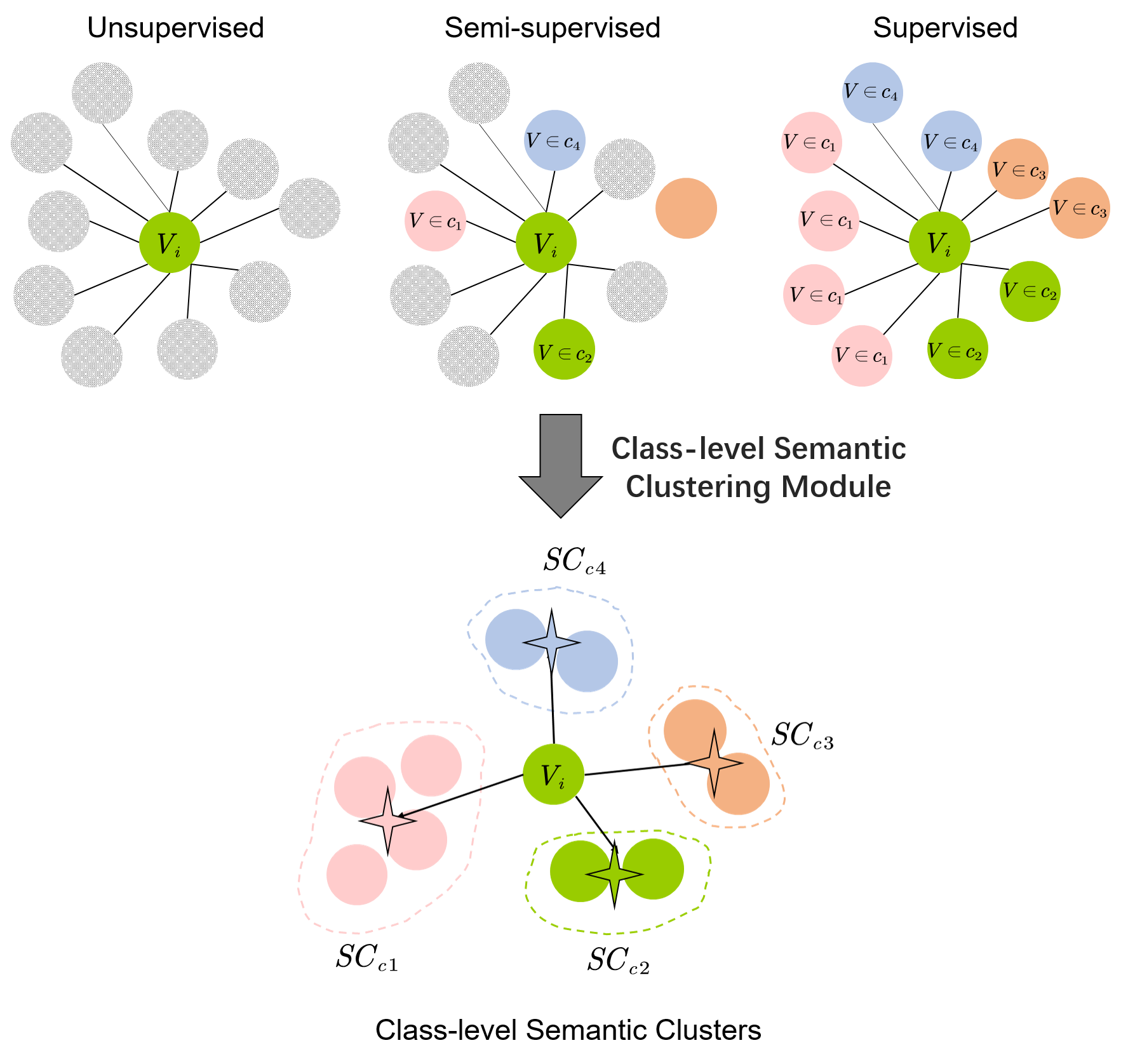
Figure 10: Three paradigms adopted in the Class-level Semantic Clustering Module.

5.3 Total Effect Estimation Module

As illustrated in Figure 9, there are two paths from class-level Semantic Clusters to the central node’s attention distribution that will jointly influence the representation learning of the central node. Therefore, we employed Total Effect as a measurement of Distraction Effect based on the preliminary of Causal Inference. This module contains three important steps, Semantic Cluster Intervention, Intervened Attention Leaning and Graph Trimming.

1. Semantic Cluster Intervention. As detailed in Section 3, Total Effect is estimated based on the intervention.This step is theoretically equivalent to asking the central node to think about a causal question: how will my attention distribution change if Semantic Cluster $c$ is removed from my LND? From the physical intuition behind this intervention-related question, it equals to a operation that renders the nodes belonging to Semantic Cluster $c$ invisible to the central node. As illustrated in Figure 11, it can be mathematically modeled as Eq.7, where $A$ represents the adjacency matrix of original graph, $\hat{A}$ represents that of intervened graph.

   $$do\left(SC_{c}=0\right):A_{ij}=1,SC(j)=c$$ (7)

   $$do\left(SC_{c}=1\right):\hat{A}_{ij}^{c}=0,SC(j)=c$$

2. Intervened Attention Learning. Since the intervention on Semantic Cluster does not affect the shape of Class-level Semantic Space (which is totally governed by the data generation mechanism of the graph), we need to guarantee that before and after the intervention, the GAT model only changes the attention distribution, while the other capabilities remain unchanged. From the perspective of model implementation, we do not alter the parameters responsible for transforming node features, allowing the model to solely relearn the allocation of attention to neighboring nodes and itself. The attention assigned to Semantic Clusters can be represented in Eq.8, where $\alpha_{SC}^{c}=\sum\limits_{SC(V_{j})=c}\alpha_{ij}$, and the self-attention of central node $V_{i}$ is $\alpha_{self\_attention}=1-\sum\limits_{C}\alpha_{SC}^{c}$.

   $$\alpha_{SC}=\left\{\alpha_{SC}^{1},\alpha_{SC}^{2},\ldots,\alpha_{SC}^{C}\right\}\in\mathbb{R}^{C\times 1}$$ (8)

3. Graph Trimming. According to the concept in Section 3, we can calculate the TE on Central node’s self-attention of Semantic Cluster $c$ according to Eq.9.

   $$\begin{split}TE_{\alpha_{self\_attention}}&=E_{\alpha_{self\_attention}\mid do\left(SC_{c}=1\right)}\left[\alpha_{self\_attention}\mid\operatorname{do}\left(SC_{c}=1\right)\right]\\ &-E_{\alpha_{self\_attention}\mid do\left(SC_{c}=0\right)}\left[\alpha_{self\_attention}\mid\operatorname{do}\left(SC_{c}=0\right)\right]\end{split}$$ (9)

   The lower the value of the sum of $TE_{\alpha_{SC}}$, which implies the higher value of $TE_{\alpha_{self\_attention}}$, the more it can distract the central node and lead to the low self-attention of the central node, and vice versa. Therefore, we remove the Semantic Cluster with lower $TE_{\alpha_{SC}}$ and only retain the Semantic Cluster with the highest $TE_{\alpha_{SC}}$. In other words, only the Semantic Cluster with the lowest TE on self-attention of the central node will remain. Eventually, we obtain the adjacency matrix of the Trim Graph denoted as Eq.10, which equals to a operation that remove the adjacent edges between Distraction Neighbors and central nodes.

   $$A_{\text{Trim}}=\left\{a_{ij}=1,SC(j)=\min\left(TE_{\alpha_{self\_attention}}\right)\right\}$$ (10)

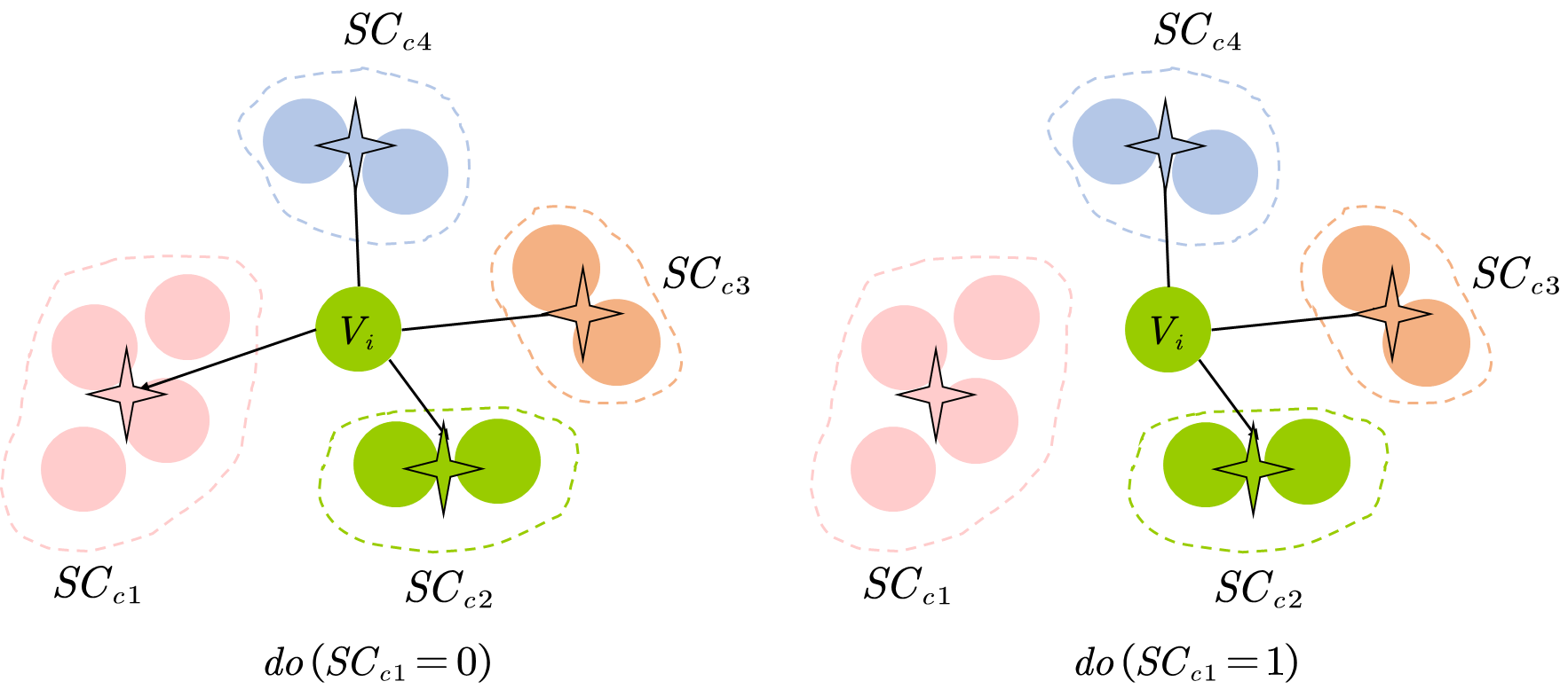
Figure 11: Semantic cluster intervention.

6 Experiments and Results

6.1 Databases

To ensure the richness and representatives of the data, we selected seven heterophilic graphs of three different sizes, each with an Edge Homophily lower than 0.23. The basic information of the dataset is given in the Table 2. The Edge Homophily is defined as Eq.11, and lower Edge Homophily indicates higher heterophily of graph.

$$H_{\text{edge }}=\frac{\left|y_{i}=y_{j},(i,j)\in E\right|}{|E|}$$ (11)

• Small-size datasets. We use the WebKB dataset [42] constructed from the WebKB webpage [58]. They are collected from computer science departments of Cornell, Texas and Wisconsin university. These datasets are built from the hyperlinks between webpages, and the features of node are the bag-of-words representation. Nodes belong to five categories.

• Medium-size datasets. We use the Chameleon and Squirrel [59] dataset collected from Wikipedia, they are applicable for node regression and node classification [42] tasks. In these datasets, the nodes represent webpages and the edges are links between them. When applied for node classification task, the target is to predict 5 classes based on the average traffic of webpages.

• Large-size datasets. We use the Roman-empire [60] constructed from Wikipedia article. In this dataset, the nodes represent words in the text and the edges are constructed from their context. The target is to predict 18 classes based on the syntactic role of the nodes.

Table 2: Statistics of the datasets.

Dataset		Nodes	Edges	Average Degree	Features	Classes	Edge Homophily
Small-size	Cornell	183	295	3.06	1703	5	0.13
	Texas	183	309	3.22	1703	5	0.11
	Wisconsin	251	499	3.71	1703	5	0.20
Medium-size	Chameleon	2277	62792	27.60	128	5	0.23
	Squirrel	5201	396846	78.33	128	5	0.22
	Actor	7600	33269	7.02	932	5	0.21
Large-size	Roman-empire	22662	65854	2.91	300	18	0.04

6.2 Experiments

We aim to explore the effect of neighboring nodes on the central node’s attention learning within the GAT mechanism. Therefore, we take the GAT with fixed architecture (which can be regarded as having the same aggregation and feature transformation ability) as the base model, and compare the discrimination ability on graph with different LND. We focus more on the difference caused by attention distribution learned by GATs, thus choosing not to tune the architecture of GATs through careful optimization and parameter tuning. In this paper, we adopted three GATs as the base model and constructed corresponding CAT variants. To distinguish the results on different base models, we replace the ’G’ in the base model name with ’C’ to represent the corresponding CAT. The base GATs and their fixed architecture are as followed:

• GAT[25]. The originally proposed Graph Attention Network. We set the layer of GAT to 2 and multi-head number to 8.

• GATv2[61]. A dynamic graph attention variant that can learn dynamic attention by simply switching the order of internal operations in GAT. We set the layer of GATv2 to 2 and multi-head number to 8.

• GATv3[47]. A new attention mechanism that calculates query and key with other GNN models in GAT framework. We set the layer of GATv3 to 2 and adopt one-layer GCN in K and Q module. To better investigate the effect of attention learning, we fix the weight of calculated attention to 1 and abandon the original weighted attention strategy.

For all base GATs and their CAT variants, we use the Adam optimizer with a learning rate of 0.001 and a weight decay of 0.0001 to train the model. A single Nvidia 2080Ti is used for training with a negative log likelihood loss. The maximum iteration is 600, and the tolerance in the early stopping strategy based on the classification accuracy on the validation set is set to 50. For the evaluation of the model accuracy, we divide the dataset into training, validation and test set with the ratio of 6:2:2, and use the average classification accuracy and standard deviation of the test set in 100 repetitions as the final evaluation metrics. We set the dimensions of the hidden layers to {16,32,64,128} and adopt the optimal classification accuracy. We conduct comparison experiment and ablation experiment to verify the validity of the architecture and single modules of CAT, respectively. Visualization experiments are also carried out for further interpretation of the results.

6.2.1 Comparison Experiment

We feed the original heterophilic graph and the trimmed graph obtained by CAT variants to the base GAT to obtain the final node classification accuracy, respectively. Trimmed graphs are obtained in three variants of CAT with the following setting:

• CAT-unsup. Since the number of Semantic Clusters is known (equal to the number of target classes), we use the K-means++ algorithm in the Class-level Semantic Clustering Module for the unsupervised manner. To avoid the influence of the initial clustering centers on the results, we use 0,10,100 as random seeds respectively for the initialed clustering centers in K-means++.

• CAT-semi. For the semi-supervised manner, we employed a two-layer Multi-Layer Perception (MLP) to learn the categorical distribution of nodes. To keep the consistency of the semi-supervised node classification task, we use the same dataset split described in Section 6.1 for the MLP.

• CAT-sup. For the supervised manner, we directly use the labels to generate the Class-level Semantic Clusters.

The results are shown in the Table 3. It can be found that our approach demonstrates improvements across all base GAT models. Even on the Large-size dataset with the Edge Homophily of only 0.04, the minimum of relative improvements for GAT and GATv2 achieve 13.5%, 10.1%, respectively. Adopting semi-supervised and fully-supervised paradigm can further enhance the improvement. GATv3 exhibits the best performance among all base models due to its incorporation of a new attention mechanism that calculates query and key from other GNN models, enhancing its discrimination capability. Despite this, CAT framework can further improve its classification accuracy. Among all base models, the relative improvement of CAT on GATv3 is the lowest. The reason is GATv3 already boasts a comparatively high level of discrimination ability and classification accuracy on heterophilic graphs, making further enhancement more challenging.

In terms of the standard deviation of the prediction accuracy, on Small-size datasets, the deviation of CATs is relatively large as the base GATs, which is caused by the smaller size of the dataset. However, on Medium-size and large-size datasets, CAT is able to significantly reduce the deviation and achieve more stable and statistically significant predictions on the dataset.

For all base GATs, CAT-sup can generally achieve the best performance than CAT-unsup and CAT-semi. It is because the more information is leveraged in the Class-level Semantic Clustering Module there by a more accurate distribution of Semantic Clusters is obtained. In the same way, this speculation can also explain why CAT-unsup performs the worst, and the CAT-semi consistently performs at a middle level. On one hand, this indicates that precise Class-level Semantic Clustering can assist the central node in better allocating attention. On the other hand, it poses a challenge to learning a more optimal Semantic Space. CAT-unsup with different random seeds also obtain significantly different performance. For example, although all CAT-unsup can outperform GAT on the Wisconsin dataset, CAT-unsup with random seed value of 10 gains over 10% lower accuracy than that with value of 100. CATv2-unsup exhibits a similar pattern on the Texas dataset. This indicates that we can barely guarantee that the learned Class-level Semantic Space is optimal or approaching optimal for the sake of unsupervised manner. Also, it indicates that the output of Class-level Semantic Clustering has a significant effect on the whole method.

Table 3: Node classification accuracy. 0,10,100 represent the corresponding random seed used in the unsupervised clustering method. The best result and worst result achieved by CAT variants are marked in bold and wave line separately, and their relative improvements compared to GAT are shown below. The base models and the worst result among all models are marked in red. OOM represents out of memory.

Dataset		Small-size			Medium-size			Large-size
($H_{edge}$)		Cornell (0.13)	Texas (0.11)	Wisconsin (0.20)	Chameleon (0.23)	Squirrel (0.22)	Actor (0.21)	Roman-empire (0.04)
GAT		60.9$\pm$3.4	49.9$\pm$2.2	53.7$\pm$2.5	44.9$\pm$1.8	21.5$\pm$1.7	28.6$\pm$0.4	54.2$\pm$0.5
CAT-unsup	0	75.8$\pm$3.5	65.2$\pm$2.4	62.5$\pm$4.3	48.8$\pm$0.6	29.0$\pm$0.3	32.6$\pm$0.6	61.5$\pm$0.2
	10	72.9$\pm$4.1	70.2$\pm$2.2	70.2$\pm$2.2	51.9$\pm$0.7	28.9$\pm$0.3	33.7$\pm$0.6	63.5$\pm$0.3
	100	69.0$\pm$2.0	69.6$\pm$3.4	69.6$\pm$3.4	51.9$\pm$1.0	28.4$\pm$0.3	31.5$\pm$0.4	62.2$\pm$0.2
CAT-semi		71.0$\pm$3.2	73.0$\pm$3.9	73.0$\pm$3.9	50.6$\pm$0.5	28.7$\pm$0.4	32.8$\pm$0.6	61.9$\pm$0.2
CAT-sup		80.4$\pm$3.0	76.7$\pm$3.1	82.0$\pm$1.6	53.4$\pm$0.9	32.4$\pm$0.9	35.5$\pm$0.5	64.4$\pm$0.2
Relative Improvement (%)		13.3-32.0	30.9-53.7	16.4-52.7	8.7-18.9	32.1-50.7	10.1-24.1	13.5-18.8
GATv2		61.1$\pm$3.6	50.2$\pm$2.2	53.8$\pm$2.4	45.9$\pm$1.6	21.4$\pm$2.1	28.5$\pm$0.4	56.5$\pm$0.8
CATv2-unsup	0	78.1$\pm$3.2	62.8$\pm$2.9	77.3$\pm$1.5	51.8$\pm$0.9	28.2$\pm$0.4	31.8$\pm$0.5	63.3$\pm$0.1
	10	74.5$\pm$4.3	75.8$\pm$1.5	79.1$\pm$2.3	52.0$\pm$0.7	28.0$\pm$0.4	32.4$\pm$0.5	62.2$\pm$0.2
	100	74.8$\pm$1.6	70.4$\pm$4.9	76.9$\pm$3.0	50.6$\pm$0.5	28.5$\pm$0.3	32.3$\pm$0.5	63.1$\pm$0.2
CATv2-semi		81.5$\pm$3.4	75.3$\pm$3.4	78.7$\pm$2.2	53.1$\pm$0.9	29.9$\pm$1.4	31.9$\pm$0.5	63.0$\pm$0.2
CATv2-sup		81.7$\pm$3.8	72.8$\pm$2.0	84.2$\pm$2.0	56.9$\pm$0.9	32.4$\pm$1.3	33.1$\pm$0.5	63.4$\pm$0.2
Relative Improvement (%)		21.9-33.7	25.1-50.0	42.9-56.5	10.2-24.0	30.8-51.4	11.6-16.1	10.1-12.2
GATv3		86.3$\pm$2.2	81.6$\pm$2.4	80.8$\pm$2.3	62.9$\pm$1.0	33.7$\pm$0.7	35.1$\pm$0.5	OOM
CATv3-unsup	0	88.2$\pm$2.0	83.1$\pm$2.9	82.3$\pm$2.5	64.2$\pm$0.8	53.7$\pm$0.9	37.8$\pm$0.6	-
	10	87.5$\pm$2.0	82.8$\pm$2.5	84.3$\pm$2.5	64.2$\pm$0.9	53.6$\pm$0.8	36.9$\pm$0.5	-
	100	88.0$\pm$2.2	83.3$\pm$3.4	83.2$\pm$2.4	63.4$\pm$0.8	53.6$\pm$0.7	38.0$\pm$0.5	-
CATv3-semi		88.4$\pm$2.1	82.8$\pm$2.7	84.6$\pm$2.2	67.1$\pm$0.8	55.9$\pm$0.8	37.7$\pm$0.6	-
CATv3-sup		88.8$\pm$2.1	83.0$\pm$2.5	85.6$\pm$2.1	69.9$\pm$1.0	59.3$\pm$1.8	38.5$\pm$1.2	-
Relative Improvement (%)		1.4-2.9	1.5-2.1	1.9-5.9	0.8-11.1	59.1-76.0	5.1-9.7	-

6.2.2 Ablation Experiment

To investigate the effectiveness of components in proposed method, we conducted ablation studies on two modules separately and obtain two corresponding trimmed graphs as input. For the sake of better comparison, we selected CAT-unsup in this section because it performs the worst among three variants of CAT thereby can better support the ablation experiments. The result of ablation experiment is shown in Table 4.

1. CAT (random_cluster). To investigate the effectiveness of the Class-level Semantic Cluster module, we replace it with a random assigned cluster module. We set the random seed of 0, 10, 100 respectively for the random cluster assignment.

2. CAT(high_distraction). To investigate the effectiveness of the Total Effect Estimation, we remove the neighbors with lower distraction and create a High Distraction and Low Self-attention scenario. This model reserves the $\max\left(TE_{\alpha_{self\_attention}}\right)$ in the Total Effect Estimation.

Table 4: The ablation experiment result. The CAT in this table represents the CAT-unsup. The best accuracy is marked in bold, and the worst is in wavy line.

Dataset	Trimmed graph	Random seed
		0	10	100
Cornell	CAT	75.8$\pm$3.5	72.9$\pm$4.1	69.0$\pm$2.0
	CAT(random_cluster)	72.4$\pm$3.2	74.1$\pm$3.2	70.4$\pm$1.7
	CAT(high_distraction)	73.3$\pm$3.0	68.9$\pm$2.1	65.2$\pm$2.4
Texas	CAT	65.2$\pm$2.4	70.2$\pm$2.2	66.6$\pm$3.4
	CAT(random_cluster)	67.4$\pm$3.1	69.5$\pm$2.1	69.5$\pm$3.6
	CAT(high_distraction)	61.9$\pm$2.9	68.4$\pm$3.1	68.4$\pm$3.1
Wisconsin	CAT	62.5$\pm$4.3	76.2$\pm$3.9	76.5$\pm$2.7
	CAT(random_cluster)	72.2$\pm$1.8	73.0$\pm$1.9	66.4$\pm$3.0
	CAT(high_distraction)	60.9$\pm$2.2	68.9$\pm$2.0	64.3$\pm$2.5
Chameleon	CAT	48.8$\pm$0.6	51.9$\pm$0.7	51.9$\pm$1.0
	CAT(random_cluster)	48.5$\pm$0.5	47.9$\pm$0.6	48.8$\pm$1.1
	CAT(high_distraction)	45.9$\pm$0.8	41.5$\pm$0.6	40.0$\pm$1.1
Squirrel	CAT	29.0$\pm$0.3	28.9$\pm$0.3	28.4$\pm$0.3
	CAT(random_cluster)	28.2$\pm$0.3	27.1$\pm$1.6	27.6$\pm$0.9
	CAT(high_distraction)	24.5$\pm$2.7	27.3$\pm$1.9	26.7$\pm$0.2
Actor	CAT	32.6$\pm$0.6	33.7$\pm$0.6	31.5$\pm$0.4
	CAT(random_cluster)	32.9$\pm$0.5	31.9$\pm$0.5	31.7$\pm$0.5
	CAT(high_distraction)	30.6$\pm$0.6	30.9$\pm$0.4	29.7$\pm$0.4
Roman-empire	CAT	61.5$\pm$0.2	63.5$\pm$0.3	62.2$\pm$0.2
	CAT(random_cluster)	61.2$\pm$0.2	61.5$\pm$0.2	61.0$\pm$0.3
	CAT(high_distraction)	48.8$\pm$0.2	51.0$\pm$0.3	49.7$\pm$0.3

It can be found that CAT always achieves the best performance, while CAT (high_distraction) gets the worst performance. This comparison supports our Low distraction and High self-attention assumption, and also proves the effectiveness of our Total Effect Estimation Module. CAT (random_cluster) gets the medium performance, indicating the significance of our Class-level Semantic Clustering Module, and to some extent it can help us learn the effect of each class on the performance of the central node in the semantic space. In addition, it also shows that Total Effect Estimation Module has a larger and more stable contribution to CAT.

However, we also notice that CAT (random_cluster) is able to achieve results comparable to or even exceeding CAT in very few cases, which suggests that the clustering results obtained by the Class-level Semantic Clustering Module need to be optimized, whereas random cluster may be better. This phenomenon is more striking on small-size dataset, and the possible reason is that this kind of dataset itself has class imbalance (as shown in Figure 12), which will raise the difficulty of clustering.

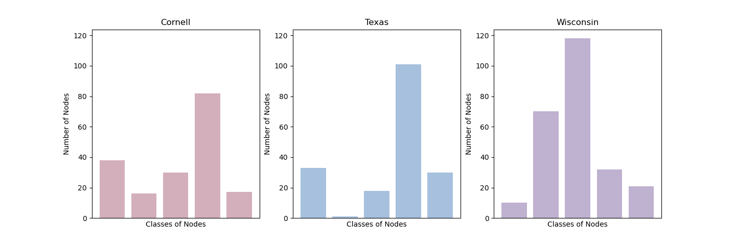
Figure 12: The class imbalance of small-size datasets.

6.2.3 Visualization

CAT can enhance the self-attention of central nodes. In order to verify whether CAT enhances the central node’s self-attention and reduces the DE it suffers, we compare the final learned self-attention of all nodes before and after trimming. We take CAT-unsup as an example and visualize the self-attention improvement in Figure 13. It can be found that for the vast majority of nodes, the Trimmed graph obtained by CAT can make GAT pay more attention to the node itself and avoid the neighbors’ distraction; while very few nodes show a decrease in self-attention, it may be due to the fact that the node already has high self-attention before trimming and the neighbors received higher attention after trimming due to the reduction of competitors. Fortunately, this situation is very rare in the dataset and does not affect the overall discrimination ability of the model.

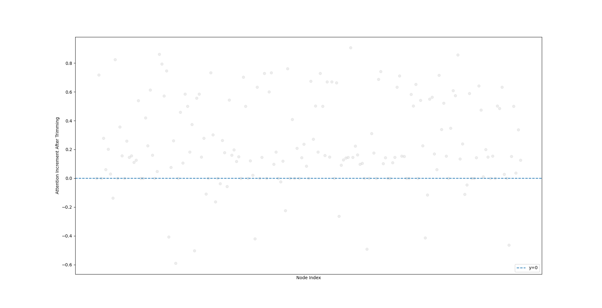
(a) Cornell

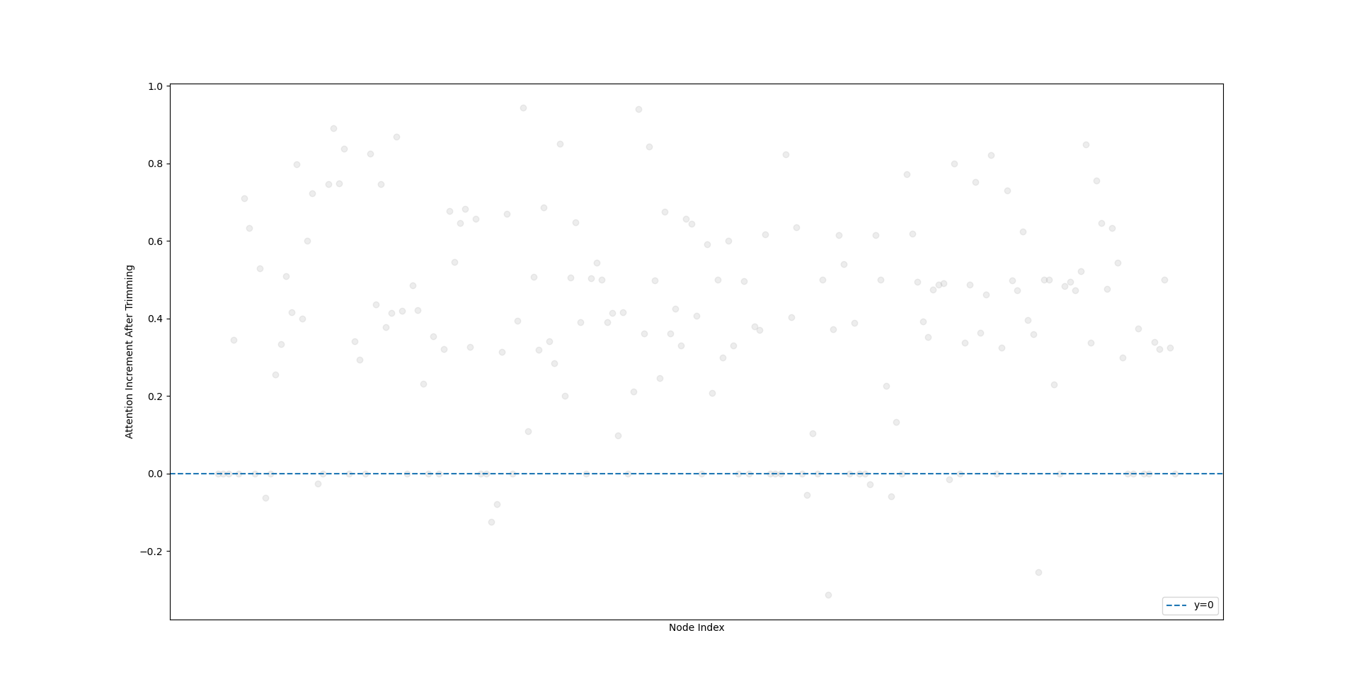
(b) Texas

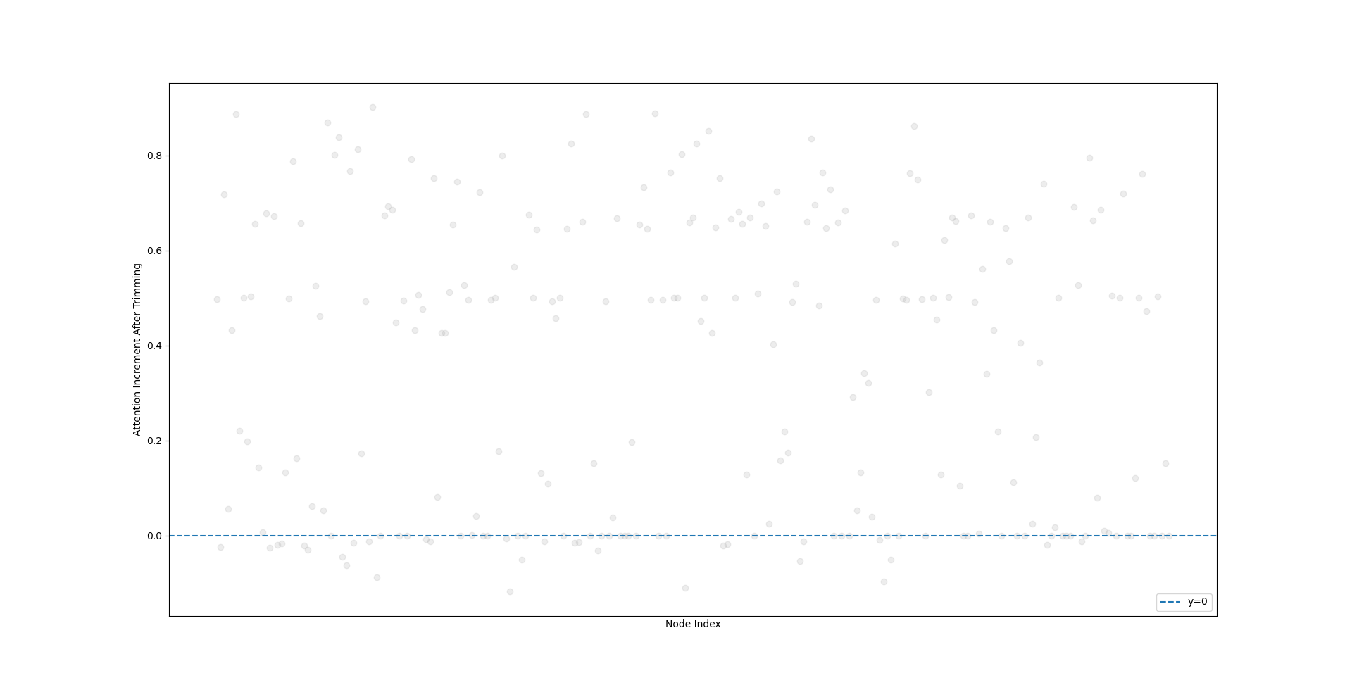
(c) Wisconsin

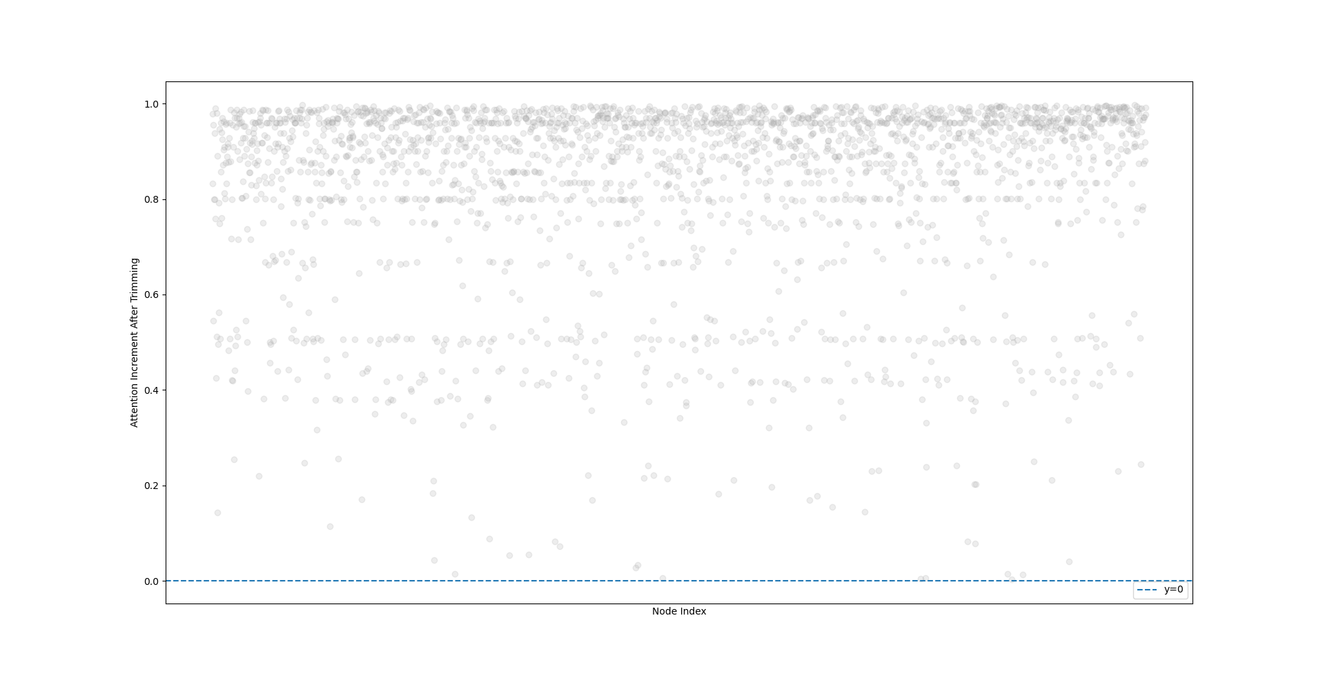
(d) Chameleon

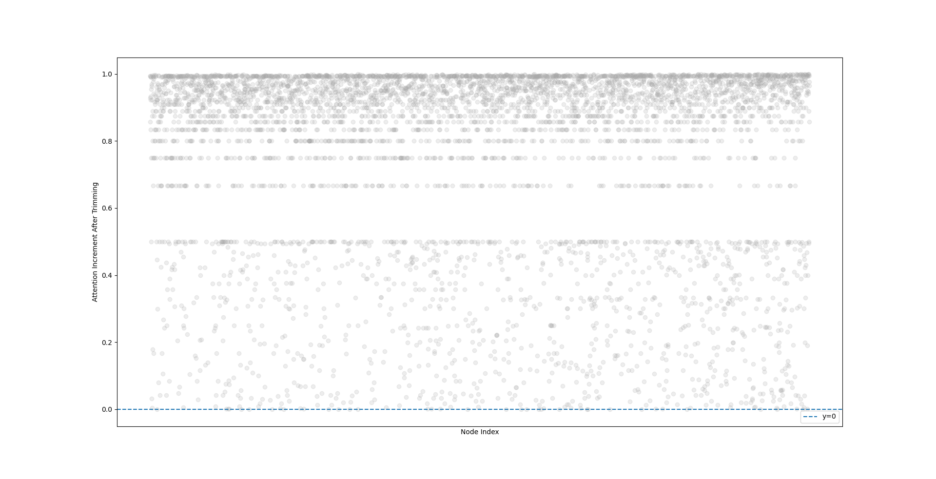
(e) Squirrel

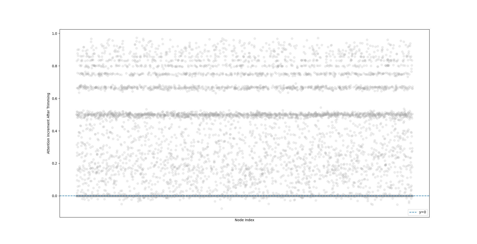
(f) Actor

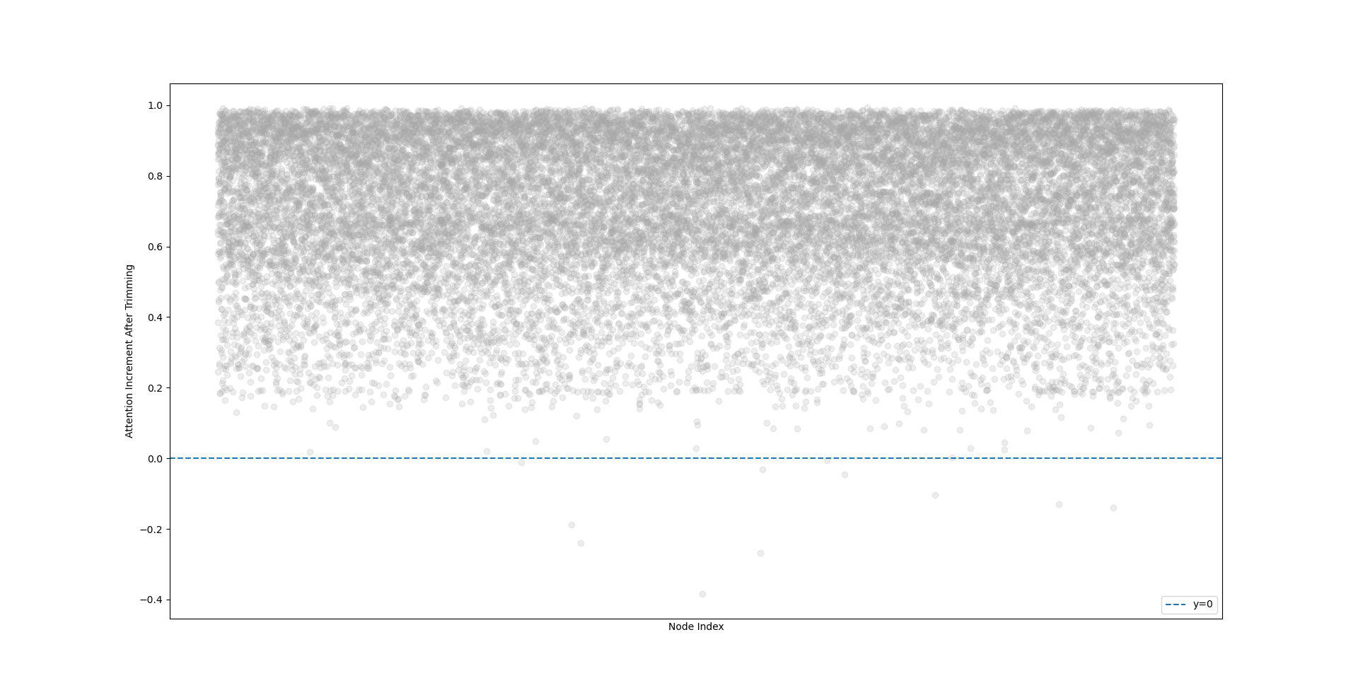
(g) Roman-empire

Figure 13: Comparison of learned self-attention before and after graph trimming. The vertical coordinate represents the change of self-attention after graph trimming ad higher value represents the more significant enhancement of the central nodes’ self-attention.

CAT can alleviate the discrimination ability degradation of GAT. In order to verify whether the model discrimination ability has been improved, we conduct dimensional reduction and visualization on the node representations learned by the model, and their corresponding Silhouette Coefficient (SC) is also calculated. As shown in Figure 14, we use TSNE to reduce the representation to two dimensions, where the higher SC represents the higher discrimination ability on different classes. We compared the original features of the data, the representations output by GAT, and the representations output by CAT variants, and compared their corresponding SC. The parameter settings with the highest node classification accuracy were chosen for both GAT and CAT as the represented result. We find that the representations obtained using GAT may involve a lower SC than the original features, where the discrimination ability degradation of GAT is manifested. In contrast, the representations obtained by CAT variants consistently get a higher SC than both the original features and the GAT representations, which implies that CAT can alleviate the discrimination ability degradation of GAT. It can be observed that the discrimination abilities of the three CAT variants are relatively close. Generally, CAT-sup demonstrates the highest discrimination capability, followed by CAT-semi, with CAT-unsup showing the lowest. Although the SC obtained by our method is still not high enough, it is enough to get some boost in rescuing the decline in discrimination ability caused by attention mechanism.

Figure 14: The Silhouette Coefficient (SC) of learned node representation. The representations obtained by CAT consistently get a higher SC than both original features and GAT representations.

CAT can map graph to a representation space that is closer to the ideal semantic space. When visualizing the dimensionality reduced representations, we found that although CAT could learn neither representation with a high SC nor easily separable boundary for heterophilic graphs, more nodes learned by CAT have a significant clustering tendency compared to GAT, which is manifested as more clustered structures in visualized figures. As shown in Figure 15, on the Chameleon dataset, CAT can identify more clusters than GAT such as the dark green and dark purple clusters. On the Cornell dataset, the node representations obtained by CAT bring nodes of the same class closer in the representation space such as the light green and dark purple clusters, which means the nodes locate closer to the cluster center and are easier to be distinguished from the clusters in other classes. As shown in Figure 16, for the same base GAT model, different CAT variants exhibit significantly distinct performances. As the base model, GATv3 learns the Semantic Cluster distribution with the lowest cluster cohesion and separation. There is an evident trend that with the more Class-level Semantic Cluster information, the variant of CAT is able to learn the clusters that are more compact and separable. It is apparently that the distances between clusters learned by CATv3-sup are maximized and nodes within a cluster is closest to the cluster center, while CATV3-unsup exhibits the opposite performance. This indicates the significance of Class-level Semantic Clusters.

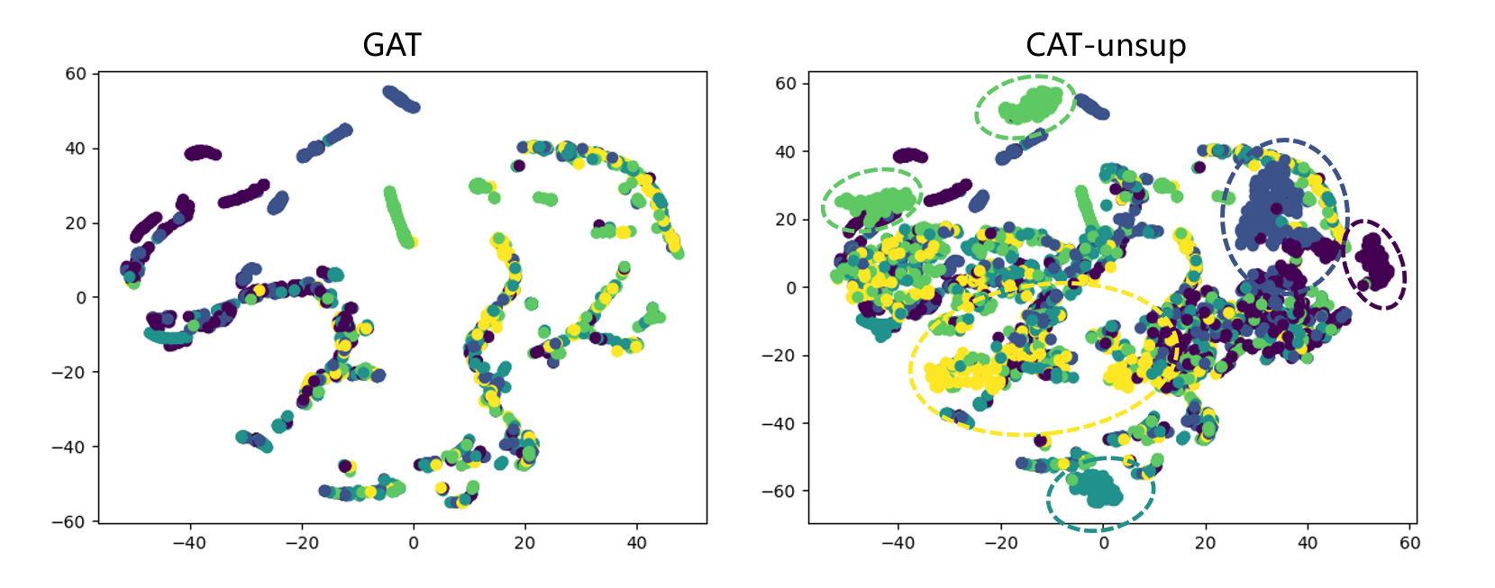
(a) Chameleon

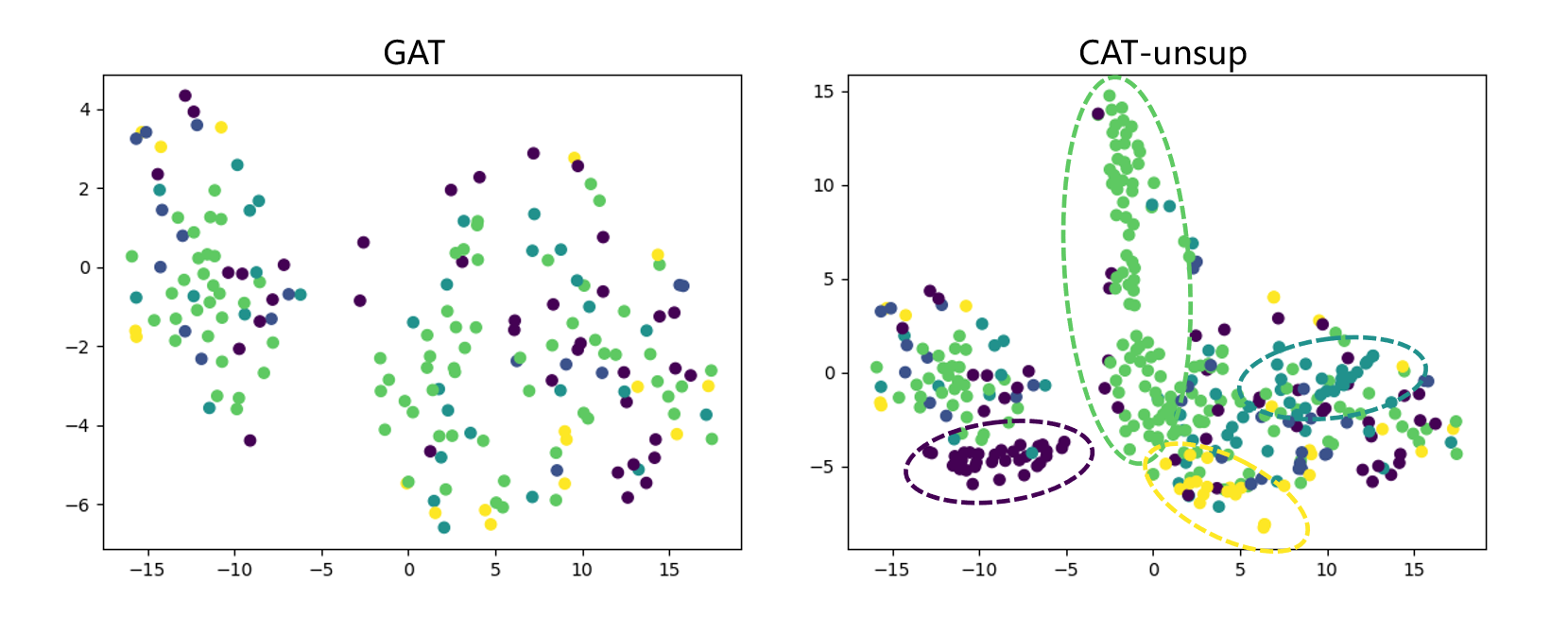
(b) Cornell

Figure 15: Visualization of embedding in the representation space learned by GAT and CAT-unsup.

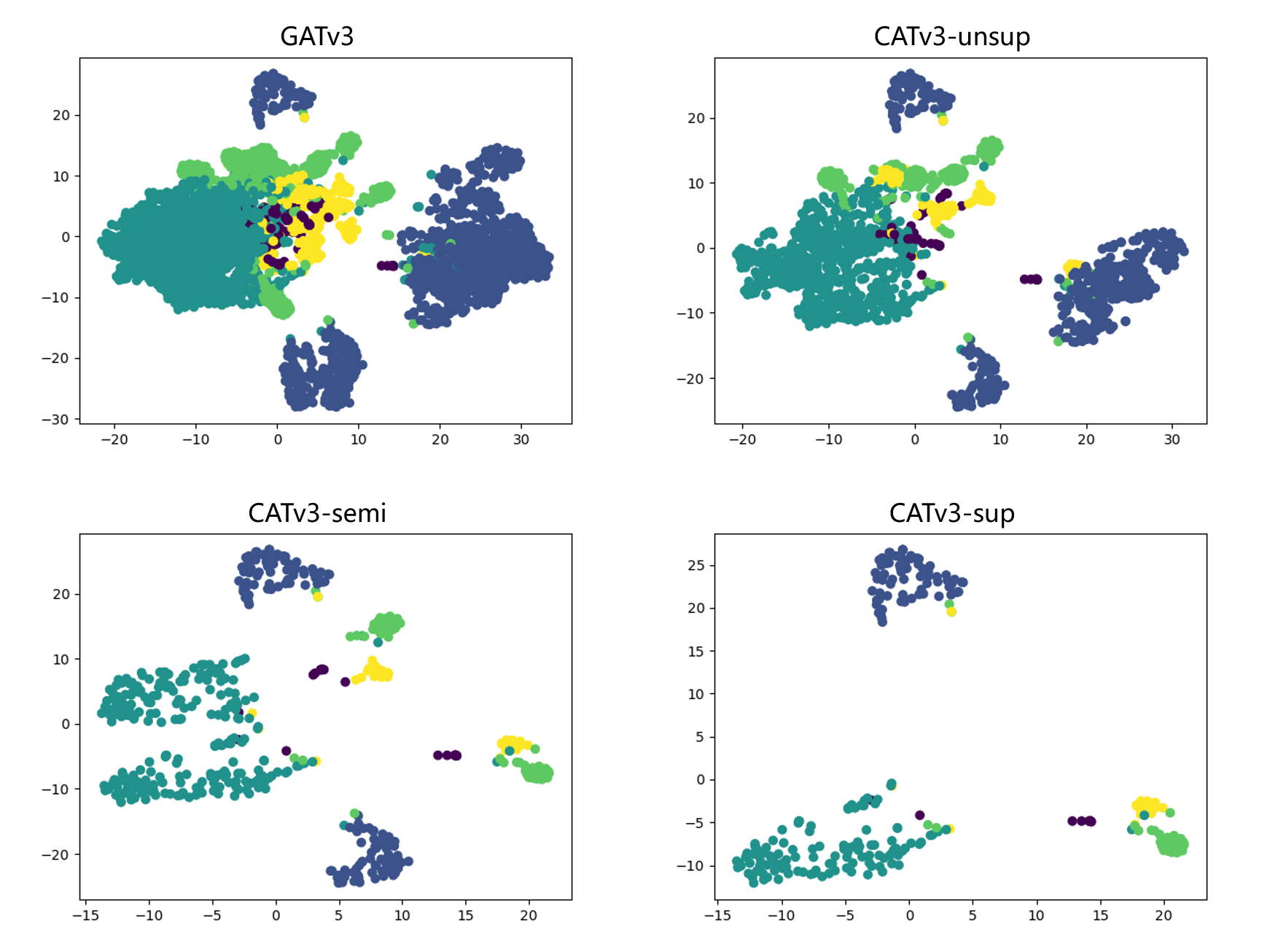
Figure 16: Visualization of embedding of Wisconsin dataset learned by GATv3, GATv3-unsup, GATv3-semi and GATv3-sup.

7 Discussions

7.1 Fundamental Hypothesis on Heterophilic Graphs

Improving the performance of GATs (GNNs as well) on the node classification task on heterophilic graphs is only a tangible task, the more fundamental issue behind improving the discrimination ability of the model is the assumption about the generation mechanism of the heterophilic graph. The Strong Homophily Hypothesis actually holds that connections between nodes are generated because they are sufficiently similar to each other, thus deriving an aggregation mechanism that relies on neighbors, which the heterophilic graphs obviously don’t hold. This can lead to an important question for heterophilic graphs, we depict this in Figure 17.

Question: what the fundamental hypothesis underlying heterophilic graphs be like? How to build better GNNs with heterophilic graphs, or how to build a brand-new graph representation learning model for heterophilic graphs, requires us to propose new inductive biases based on the heterophilic graphs’ generation mechanism [62]. This will be a challenging, landmark mission.

7.2 Limitations of CAT and Future Works

The lack of general hypothesis for heterophilic graphs. In this paper, we do not answer the question proposed in Section 7.1 directly in terms of the mechanism of data generation, but we anticipate that the model mechanism derived should be quite different from the existing Neighborhood Aggregation. Based on this insight, we tentatively offered a possible way, and have made a preliminary attempt on GAT: to make the model learn not to rely on all of its neighbors, but to concentrate on itself. Specifically, we employ causal inference as a tool to identify those neighbors that can help GAT concentrate more on the central node itself as much as possible. Our solution relies on the attention mechanism of GAT, which is not a generalized solution. How to derive a general heterophilic graph representation learning framework is an endeavor in the future.

The lack of an effective way to learn optimal class-level Semantic Cluster. According to our Class-level Semantic Space Hypothesis, the ideal semantic space is supposed to be compact and separable where the Semantic Clusters can be located accurately. In Table 3, the comparison between CAT with different paradigms shows that supervised Semantic Clustering methods are more effective for learning class-level Semantic Clusters. However, considering the semi-supervised learning paradigm of node classification tasks, the Class-level Semantic Clustering Module adopting unsupervised or semi-supervised manner will be more reasonable. The challenge is the high dimensionality, sparsity, and low semantic expressiveness of node features in the dataset, posing a challenge for unsupervised and semi-supervised clustering methods to map graph nodes to an ideal semantic space. Therefore, it is challenging for unsupervised and semi-supervised clustering methods to map graph nodes to an ideal semantic space. More effective methods to learn better Class-level Semantic Space using less label information should be explored in the future, including unsupervised, semi-supervised and self-supervised learning methods. Training self-adaption modules is also an effective way to be considered.

The lack of extension to Transformer-based graph learning methods. Since we only investigate the discrimination ability degradation of GNNs when meeting heterophilic graphs caused by the local attention-guided message passing mechanism, our framework is specifically designed for GATs. However, the Transformer [63], as a powerful neural network capable of handling sequential data, with its ability to capture global attention, can be transferred to graph learning tasks with a more powerful attention mechanism. Whether Graph Transformers [64, 65, 66] face the same challenges as GATs on heterophilic graphs, and how to extend the strategy behind this work to the Graph Transformer architecture are directions for future exploration.

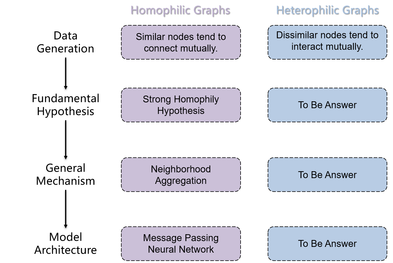
Figure 17: Discussion on heterophilic graphs.

8 Conclusion

In order to cope with the significant degradation of node classification performance of GATs on heterophilic graphs, we propose a graph trimming method applied on GAT framework, Causally graph Attention network for Trimming heterophilic graph (CAT). Three representative GATs are employed as the base model and their discrimination ability can be significantly improved after trimming the graph by CAT. Specifically, we propose a new hypothesis for GATs on heterophilic graphs, Low Distraction and High Self-Attention, arguing that enabling the central node to concentrate on itself and reduce distraction from a portion of neighbors is an effective way to avoid degradation of discrimination ability of GATs. Based on this hypothesis, we use the attention distribution learned on the original graph as a signal to estimate the distraction caused by neighbors with the help of causal inference method, and then identify the Distraction Neighbors. Distraction Neighbors are further removed in the way of graph trimming, allowing the GAT model to achieve better node classification performance by maintaining self-attention. Compared with existing methods, our method eliminates the need to alter the model architecture of GAT or searching for more neighbors globally in the graph, but learns a new graph structure in the process of learning attention to get a better attention distribution. The experimental results show that our method is able to achieve a significant improvement in the performance of the node classification task for GATs on a total of seven heterophilic graphs in three different sizes. In addition, the framework of our method can be applied to any LAMP-driven models.

References

- [1] Nan Jiang, Bo Ning, and Jingyang Dong. A survey of gnn-based graph similarity learning. In 2023 8th International Conference on Image, Vision and Computing (ICIVC), pages 650–654, 2023.
- [2] Chen Gao, Xiang Wang, Xiangnan He, and Yong Li. Graph neural networks for recommender system. In Proceedings of the Fifteenth ACM International Conference on Web Search and Data Mining, WSDM ’22, page 1623–1625, New York, NY, USA, 2022. Association for Computing Machinery.
- [3] Xiang Wang, Xiangnan He, Yixin Cao, Meng Liu, and Tat-Seng Chua. Kgat: Knowledge graph attention network for recommendation. In Proceedings of the 25th ACM SIGKDD International Conference on Knowledge Discovery & Data Mining, KDD ’19, page 950–958, New York, NY, USA, 2019. Association for Computing Machinery.
- [4] Hongwei Wang, Fuzheng Zhang, Mengdi Zhang, Jure Leskovec, Miao Zhao, Wenjie Li, and Zhongyuan Wang. Knowledge-aware graph neural networks with label smoothness regularization for recommender systems. In Proceedings of the 25th ACM SIGKDD International Conference on Knowledge Discovery & Data Mining, KDD ’19, page 968–977, New York, NY, USA, 2019. Association for Computing Machinery.
- [5] Rex Ying, Ruining He, Kaifeng Chen, Pong Eksombatchai, William L. Hamilton, and Jure Leskovec. Graph convolutional neural networks for web-scale recommender systems. In Proceedings of the 24th ACM SIGKDD International Conference on Knowledge Discovery & Data Mining, KDD ’18, page 974–983, New York, NY, USA, 2018. Association for Computing Machinery.
- [6] Chen Gao, Yu Zheng, Nian Li, Yinfeng Li, Yingrong Qin, Jinghua Piao, Yuhan Quan, Jianxin Chang, Depeng Jin, Xiangnan He, and Yong Li. A survey of graph neural networks for recommender systems: Challenges, methods, and directions. ACM Trans. Recomm. Syst., 1(1), mar 2023.
- [7] H. Xu, C. Jiang, X. Liang, and Z. Li. Spatial-aware graph relation network for large-scale object detection. In 2019 IEEE/CVF Conference on Computer Vision and Pattern Recognition (CVPR), pages 9290–9299, Los Alamitos, CA, USA, jun 2019. IEEE Computer Society.
- [8] Danfeng Hong, Lianru Gao, Jing Yao, Bing Zhang, Antonio Plaza, and Jocelyn Chanussot. Graph convolutional networks for hyperspectral image classification. IEEE Transactions on Geoscience and Remote Sensing, 59(7):5966–5978, 2020.
- [9] Xiaolong Wang and Abhinav Gupta. Videos as space-time region graphs. In Proceedings of the European conference on computer vision (ECCV), pages 399–417, 2018.
- [10] Runhao Zeng, Wenbing Huang, Mingkui Tan, Yu Rong, Peilin Zhao, Junzhou Huang, and Chuang Gan. Graph convolutional networks for temporal action localization. In Proceedings of the IEEE/CVF international conference on computer vision, pages 7094–7103, 2019.
- [11] Lingfei Wu, Yu Chen, Kai Shen, Xiaojie Guo, Hanning Gao, Shucheng Li, Jian Pei, Bo Long, et al. Graph neural networks for natural language processing: A survey. Foundations and Trends® in Machine Learning, 16(2):119–328, 2023.
- [12] Vassilis N Ioannidis, Antonio G Marques, and Georgios B Giannakis. Graph neural networks for predicting protein functions. In 2019 IEEE 8th International Workshop on Computational Advances in Multi-Sensor Adaptive Processing (CAMSAP), pages 221–225. IEEE, 2019.
- [13] Vladimir Gligorijević, P Douglas Renfrew, Tomasz Kosciolek, Julia Koehler Leman, Daniel Berenberg, Tommi Vatanen, Chris Chandler, Bryn C Taylor, Ian M Fisk, Hera Vlamakis, et al. Structure-based protein function prediction using graph convolutional networks. Nature communications, 12(1):3168, 2021.
- [14] Leilei Liu, Yi Ma, Xianglei Zhu, Yaodong Yang, Xiaotian Hao, Li Wang, and Jiajie Peng. Integrating sequence and network information to enhance protein-protein interaction prediction using graph convolutional networks. In 2019 IEEE International Conference on Bioinformatics and Biomedicine (BIBM), pages 1762–1768. IEEE, 2019.
- [15] Marc Brockschmidt. Gnn-film: Graph neural networks with feature-wise linear modulation. In International Conference on Machine Learning, pages 1144–1152. PMLR, 2020.
- [16] Jiawei Zhu, Qiongjie Wang, Chao Tao, Hanhan Deng, Ling Zhao, and Haifeng Li. Ast-gcn: Attribute-augmented spatiotemporal graph convolutional network for traffic forecasting. IEEE Access, 9:35973–35983, 2021.
- [17] Jiawei Zhu, Xing Han, Hanhan Deng, Chao Tao, Ling Zhao, Pu Wang, Tao Lin, and Haifeng Li. Kst-gcn: A knowledge-driven spatial-temporal graph convolutional network for traffic forecasting. IEEE Transactions on Intelligent Transportation Systems, 23(9):15055–15065, 2022.
- [18] Bing Yu, Haoteng Yin, and Zhanxing Zhu. Spatio-temporal graph convolutional networks: A deep learning framework for traffic forecasting. In Proceedings of the 27th International Joint Conference on Artificial Intelligence (IJCAI), 2018.
- [19] Ling Zhao, Yujiao Song, Chao Zhang, Yu Liu, Pu Wang, Tao Lin, Min Deng, and Haifeng Li. T-gcn: A temporal graph convolutional network for traffic prediction. IEEE transactions on intelligent transportation systems, 21(9):3848–3858, 2019.
- [20] Guimin Dong, Mingyue Tang, Zhiyuan Wang, Jiechao Gao, Sikun Guo, Lihua Cai, Robert Gutierrez, Bradford Campbel, Laura E. Barnes, and Mehdi Boukhechba. Graph neural networks in iot: A survey. ACM Trans. Sen. Netw., 19(2), apr 2023.
- [21] Kyungwoo Song, Hojun Park, Junggu Lee, Arim Kim, and Jaehun Jung. Covid-19 infection inference with graph neural networks. Scientific Reports, 13(1):11469, 2023.
- [22] Justin Gilmer, Samuel S Schoenholz, Patrick F Riley, Oriol Vinyals, and George E Dahl. Message passing neural networks. Machine learning meets quantum physics, pages 199–214, 2020.
- [23] Justin Gilmer, Samuel S Schoenholz, Patrick F Riley, Oriol Vinyals, and George E Dahl. Neural message passing for quantum chemistry. In International conference on machine learning, pages 1263–1272. PMLR, 2017.
- [24] Yao Ma, Xiaorui Liu, Neil Shah, and Jiliang Tang. Is homophily a necessity for graph neural networks? In International Conference on Learning Representations, 2022.
- [25] Petar Velickovic, Guillem Cucurull, Arantxa Casanova, Adriana Romero, Pietro Lio, Yoshua Bengio, et al. Graph attention networks. stat, 1050(20):10–48550, 2017.
- [26] Liang Yang, Mengzhe Li, Liyang Liu, Chuan Wang, Xiaochun Cao, Yuanfang Guo, et al. Diverse message passing for attribute with heterophily. Advances in Neural Information Processing Systems, 34:4751–4763, 2021.
- [27] Jiong Zhu, Ryan A Rossi, Anup Rao, Tung Mai, Nedim Lipka, Nesreen K Ahmed, and Danai Koutra. Graph neural networks with heterophily. In Proceedings of the AAAI conference on artificial intelligence, volume 35(12), pages 11168–11176, 2021.
- [28] Enyan Dai, Shijie Zhou, Zhimeng Guo, and Suhang Wang. Label-wise graph convolutional network for heterophilic graphs. In Learning on Graphs Conference, pages 26–1. PMLR, 2022.
- [29] Shengbo Gong, Jiajun Zhou, Chenxuan Xie, and Qi Xuan. Neighborhood homophily-guided graph convolutional network. arXiv preprint arXiv:2301.09851, 2023.
- [30] Yunchong Song, Chenghu Zhou, Xinbing Wang, and Zhouhan Lin. Ordered gnn: Ordering message passing to deal with heterophily and over-smoothing. In International Conference on Learning Representations, 2023.
- [31] Yujun Yan, Milad Hashemi, Kevin Swersky, Yaoqing Yang, and Danai Koutra. Two sides of the same coin: Heterophily and oversmoothing in graph convolutional neural networks. In 2022 IEEE International Conference on Data Mining (ICDM), pages 1287–1292. IEEE, 2022.
- [32] Eli Chien, Jianhao Peng, Pan Li, and Olgica Milenkovic. Adaptive universal generalized pagerank graph neural network. In International Conference on Learning Representations, 2021.
- [33] Xin Zheng, Miao Zhang, Chunyang Chen, Qin Zhang, Chuan Zhou, and Shirui Pan. Auto-heg: Automated graph neural network on heterophilic graphs. In Proceedings of the ACM Web Conference 2023, WWW ’23, page 611–620, New York, NY, USA, 2023. Association for Computing Machinery.
- [34] Jiong Zhu, Yujun Yan, Lingxiao Zhao, Mark Heimann, Leman Akoglu, and Danai Koutra. Beyond homophily in graph neural networks: Current limitations and effective designs. Advances in neural information processing systems, 33:7793–7804, 2020.
- [35] Lanning Wei, Zhiqiang He, Huan Zhao, and Quanming Yao. Enhancing intra-class information extraction for heterophilous graphs: One neural architecture search approach. arXiv preprint arXiv:2211.10990, 2022.
- [36] Wenhan Yang and Baharan Mirzasoleiman. Contrastive learning under heterophily. arXiv preprint arXiv:2303.06344, 2023.
- [37] Bei Lin, You Li, Ning Gui, Zhuopeng Xu, and Zhiwu Yu. Multi-view graph representation learning beyond homophily. ACM Transactions on Knowledge Discovery from Data, 2023.
- [38] Wei Jin, Tyler Derr, Yiqi Wang, Yao Ma, Zitao Liu, and Jiliang Tang. Node similarity preserving graph convolutional networks. In Proceedings of the 14th ACM international conference on web search and data mining, pages 148–156, 2021.
- [39] Tianmeng Yang, Yujing Wang, Zhihan Yue, Yaming Yang, Yunhai Tong, and Jing Bai. Graph pointer neural networks. In Proceedings of the AAAI conference on artificial intelligence, volume 36(8), pages 8832–8839, 2022.
- [40] Di Jin, Zhizhi Yu, Cuiying Huo, Rui Wang, Xiao Wang, Dongxiao He, and Jiawei Han. Universal graph convolutional networks. Advances in Neural Information Processing Systems, 34:10654–10664, 2021.
- [41] Mengying Jiang, Guizhong Liu, Yuanchao Su, and Xinliang Wu. Gcn-sl: Graph convolutional networks with structure learning for graphs under heterophily. arXiv preprint arXiv:2105.13795, 2021.
- [42] Hongbin Pei, Bingzhe Wei, Kevin Chen-Chuan Chang, Yu Lei, and Bo Yang. Geom-gcn: Geometric graph convolutional networks. In International Conference on Learning Representations, 2020.
- [43] Wendong Bi, Lun Du, Qiang Fu, Yanlin Wang, Shi Han, and Dongmei Zhang. Make heterophily graphs better fit gnn: A graph rewiring approach. arXiv preprint arXiv:2209.08264, 2022.
- [44] Meng Liu, Zhengyang Wang, and Shuiwang Ji. Non-local graph neural networks. IEEE transactions on pattern analysis and machine intelligence, 44(12):10270–10276, 2021.
- [45] Tao Wang, Di Jin, Rui Wang, Dongxiao He, and Yuxiao Huang. Powerful graph convolutional networks with adaptive propagation mechanism for homophily and heterophily. In Proceedings of the AAAI conference on artificial intelligence, volume 36(4), pages 4210–4218, 2022.
- [46] Shouheng Li, Dongwoo Kim, and Qing Wang. Restructuring graph for higher homophily via learnable spectral clustering. arXiv preprint arXiv:2206.02386, 2022.
- [47] Yi Guo, Xupeng Miao, and Bin CUI. Are graph attention networks attentive enough? rethinking graph attention by capturing homophily and heterophily, 2023.
- [48] Junfu Wang, Yuanfang Guo, Liang Yang, and Yunhong Wang. Heterophily-aware graph attention network. arXiv preprint arXiv:2302.03228, 2023.
- [49] Chang Li and Dan Goldwasser. Encoding social information with graph convolutional networks forpolitical perspective detection in news media. In Proceedings of the 57th Annual Meeting of the Association for Computational Linguistics, pages 2594–2604, 2019.
- [50] Andrew Kachites McCallum, Kamal Nigam, Jason Rennie, and Kristie Seymore. Automating the construction of internet portals with machine learning. Information Retrieval, 3:127–163, 2000.
- [51] C Lee Giles, Kurt D Bollacker, and Steve Lawrence. Citeseer: An automatic citation indexing system. In Proceedings of the third ACM conference on Digital libraries, pages 89–98, 1998.
- [52] Kathi Canese and Sarah Weis. Pubmed: the bibliographic database. The NCBI handbook, 2(1), 2013.
- [53] Lingfei Wu, Peng Cui, Jian Pei, and Liang Zhao. Graph Neural Networks: Foundations, Frontiers, and Applications. Springer Singapore, Singapore, 2022.
- [54] Judea Pearl and Dana Mackenzie. The book of why: the new science of cause and effect. Basic books, 2018.
- [55] Thomas N Kipf and Max Welling. Semi-supervised classification with graph convolutional networks. arXiv preprint arXiv:1609.02907, 2016.
- [56] Will Hamilton, Zhitao Ying, and Jure Leskovec. Inductive representation learning on large graphs. Advances in neural information processing systems, 30, 2017.
- [57] Haifeng Li, Jun Cao, Jiawei Zhu, Qing Zhu, and Guohua Wu. Graph information vanishing phenomenon inimplicit graph neural networks. arXiv preprint arXiv:2103.01770, 2021.
- [58] Rayid Ghani, Rosie Jones, Andrew McCallum, Tom Mitchell, Dunja Mladenic, Kamal Nigam, and Sean Slattery. Cmu world wide knowledge base (webkb) project.
- [59] Benedek Rozemberczki, Carl Allen, and Rik Sarkar. Multi-scale attributed node embedding. Journal of Complex Networks, 9(2):cnab014, 2021.
- [60] Oleg Platonov, Denis Kuznedelev, Michael Diskin, Artem Babenko, and Liudmila Prokhorenkova. A critical look at the evaluation of gnns under heterophily: Are we really making progress? In International Conference on Learning Representations, 2023.
- [61] Shaked Brody, Uri Alon, and Eran Yahav. How attentive are graph attention networks? In International Conference on Learning Representations, 2022.
- [62] Anirudh Goyal and Yoshua Bengio. Inductive biases for deep learning of higher-level cognition. Proceedings of the Royal Society A, 478(2266):20210068, 2022.
- [63] Ashish Vaswani, Noam Shazeer, Niki Parmar, Jakob Uszkoreit, Llion Jones, Aidan N Gomez, Łukasz Kaiser, and Illia Polosukhin. Attention is all you need. Advances in neural information processing systems, 30, 2017.
- [64] Erxue Min, Runfa Chen, Yatao Bian, Tingyang Xu, Kangfei Zhao, Wenbing Huang, Peilin Zhao, Junzhou Huang, Sophia Ananiadou, and Yu Rong. Transformer for graphs: An overview from architecture perspective. arXiv preprint arXiv:2202.08455, 2022.
- [65] Chengxuan Ying, Tianle Cai, Shengjie Luo, Shuxin Zheng, Guolin Ke, Di He, Yanming Shen, and Tie-Yan Liu. Do transformers really perform badly for graph representation? Advances in Neural Information Processing Systems, 34:28877–28888, 2021.
- [66] Zhanghao Wu, Paras Jain, Matthew Wright, Azalia Mirhoseini, Joseph E Gonzalez, and Ion Stoica. Representing long-range context for graph neural networks with global attention. Advances in Neural Information Processing Systems, 34:13266–13279, 2021.