Uplifting the Expressive Power of Graph Neural Networks
through Graph Partitioning
Asela Hevapathige ¹, Qing Wang¹
1 School of Computing, Australian National University, Canberra, Australia
asela.hevapathige@anu.edu.au, qing.wang@anu.edu.au

Abstract

Graph Neural Networks (GNNs) have paved its way for being a cornerstone in graph related learning tasks. From a theoretical perspective, the expressive power of GNNs is primarily characterised according to their ability to distinguish non-isomorphic graphs. It is a well-known fact that most of the conventional GNNs are upper-bounded by Weisfeiler-Lehman graph isomorphism test (1-WL). In this work, we study the expressive power of graph neural networks through the lens of graph partitioning. This follows from our observation that permutation invariant graph partitioning enables a powerful way of exploring structural interactions among vertex sets and subgraphs, and can help uplifting the expressive power of GNNs efficiently. Based on this, we first establish a theoretical connection between graph partitioning and graph isomorphism. Then we introduce a novel GNN architecture, namely Graph Partitioning Neural Networks (GPNNs). We theoretically analyse how a graph partitioning scheme and different kinds of structural interactions relate to the $k$-WL hierarchy. Empirically, we demonstrate its superior performance over existing GNN models in a variety of graph benchmark tasks.

Introduction

Graph Neural Networks (GNNs) have become the de facto paradigm in graph learning tasks (Horn et al. 2021; Bodnar et al. 2021; Bouritsas et al. 2022). Among numerous GNN models in the literature, Message-Passing Neural Network (MPNN) is a primary choice for many real-world applications due to its simplicity and efficiency. MPNNs use local neighborhood information of each node through a message-passing scheme to retrieve node representations in an iterative manner (Gilmer et al. 2017; Kipf and Welling 2016).

However, the representational power of MPNNs is well known to be upper-bounded by the Weisfeiler-Lehman test (1-WL) (Weisfeiler and Leman 1968; Xu et al. 2018; Morris et al. 2019). Various attempts have been made to enhance the expressivity of MPNNs going beyond 1-WL test, such as structural property injection (Bouritsas et al. 2022; Barceló et al. 2021; Wijesinghe and Wang 2022), consideration of higher-order substructures (Morris et al. 2019; Morris, Rattan, and Mutzel 2020; Abu-El-Haija et al. 2019), use enhanced receptive fields for message-passing (Nikolentzos, Dasoulas, and Vazirgiannis 2020; Feng et al. 2022; Wang et al. 2022), utilization of subgraphs(Zhao et al. 2021; Zhang and Li 2021; Wang and Zhang 2022; Bevilacqua et al. 2021; Cotta, Morris, and Ribeiro 2021), and inductive coloring (You et al. 2021; Huang et al. 2022).

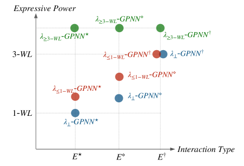
Figure 1: Expressive Power of GPNN variants: (1) Interaction type: The expressivity of GPNN is changed when considering different types of interactions (i.e., $E^{\star}$, $E^{\diamond}$, and $E^{\dagger}$) or different graph partitioning schemes (i.e., $\lambda_{\bot}$, $\lambda_{\leq 1\text{-}WL}$, and $\lambda_{\geq 3\text{-}WL}$). (2) Expressive Power: Different GPNN variants are aligned with different levels in $k$-WL hierarchy, depending on interaction types and graph partition schemes being used. All related theoretical results are elaborated in Section ”Theoretical Analysis”.

Despite various advances in expressive GNNs, there is still little understanding of how different kinds of structural components in a graph (e.g., subgraphs that capture different graph properties) interact with each other and how such interactions may influence the expressivity of graph representations for learning tasks. Existing works are mostly restricted to learning representations through simple interactions between vertices and their neighbors, thereby lacking the ability to unravel intricate interactions among structural components of different characteristics.

Present work.  This work aims to address the aforementioned limitations. Our key observations are that partitioning a graph into a set of subgraphs that preserve structural properties enables a powerful way to exploit interactions among different structural components of a graph. Particularly, graphs in real-world applications are often composed of different kinds of structural components that can be distinguished with respect to their topological properties. Exploring these structural components and their interactions can bring in novel insights about structure of a graph as well as additional power for graph representations.

Inspired by these observations, we study how permutation invariant graph partitioning can be leveraged to uplift the expressive power of GNNs efficiently. We first formalize the notion of permutation-invariant graph partitioning and then show that permutation-invariant graph partitioning can reveal intricate structural interactions between structural components. Our main contributions are summarized as follows.

• We establish a theoretical connection between graph partitioning and graph isomorphism. Two weaker notions of isomorphism on graphs, partition isomorphism and interaction isomorphism, are formulated from a permutation invariant graph partitioning perspective.

• We propose a novel GNN architecture, Graph Partitioning Neural Network (GPNN), which integrates structural interactions into graph representation learning via a permutation invariant graph partitioning scheme.

• We prove that even with graph partitioning schemes that are less expressive than 1-WL, our GNN architecture can not only go beyond 1-WL, but also achieve a good balance between expressivity, efficiency, and simplicity through exploiting different types of structural interactions.

Figure 1 illustrates the theoretical results of the proposed model GPNN in relating to $k$-WL, when considering different types of interactions and graph partitioning schemes (see details in Section “Theoretical Analysis”). To empirically verify the theoretical designs of GPNN, we conduct experiments on graph benchmark tasks, demonstrating its superior performance over state-of-the-art models (see details in Section “Experiments”.).

Related work.  There are a variety of GNN models proposed in the literature which enhance the expressive power of MPNNs to go beyond 1-WL. Some of these models extract structural information using a pre-processing step and inject it into a message-passing scheme as node or edge features (Horn et al. 2021; Barceló et al. 2021; Bouritsas et al. 2022; Wijesinghe and Wang 2022). These GNNs have been empirically verified to perform well on graphs that exhibit specific structural patterns but often require hand-pick such structure patterns. $k$-WL algorithm (Kiefer 2020; Cai, Fürer, and Immerman 1992) inspired the development of high-order GNNs that can capture higher-order relations by characterizing $k$-tuples of vertices in graphs (Maron et al. 2019b; Morris et al. 2019; Morris, Rattan, and Mutzel 2020; Zhao, Shah, and Akoglu 2022). Despite being powerful in theory, these models suffer from high computational complexity, making them futile for real-world tasks. We refer the reader to the survey articles by Sato (2020), and Zhang et al. (2023) for detailed discussion on expressive GNNs.

Previously, graph partitioning has been studied in relation to GNNs primarily for speeding up large-scale graph processing  (Xu et al. 2021; Mu et al. 2023; Gaunt et al. 2018; Miao et al. 2021; Chiang et al. 2019). Gaunt et al. (2018) uses graph partitioning to break a graph into multiple subgraphs to reduce the processing time of GNNs. They introduce a local propagation mechanism to pass messages between vertices in subgraphs and a global propagation scheme to pass messages within subgraphs. Mu et al. (2023) proposes a framework that utilizes graph partitioning for distributed GNN training. Chiang et al. (2019) clusters large-scale graphs through graph partitioning to reduce the training complexities of GNNs.

Our work is fundamentally different from existing works which partition graphs for speeding up processing. Instead, we leverage graph partition to reveal structural interactions within and between different structural components, and then encode such structure intersections into graph representations. To the best of our knowledge, this is the first work to explore the relationship between graph partitioning and graph isomorphism from the perspective of enhancing the expressive power of GNNs.

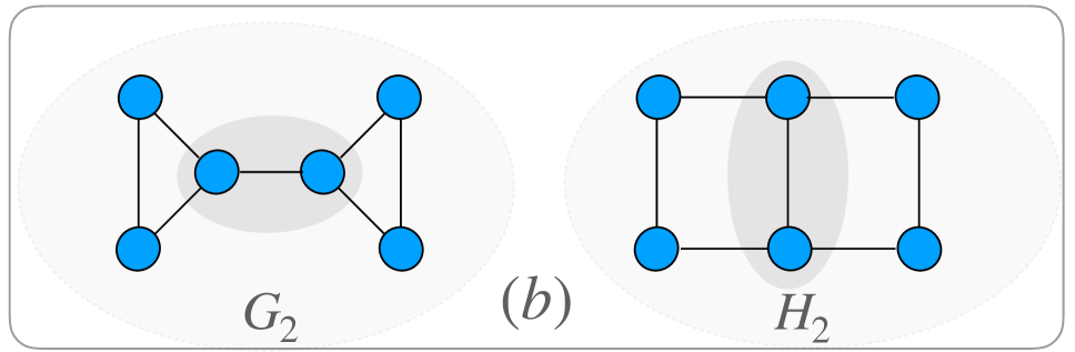
Example Graphs	GI	II	PI
(a) $G_{1}$ and $H_{1}$	✗	✓	✓
(b) $G_{2}$ and $H_{2}$	✗	✗	✓

Figure 2: Two pairs of example graphs which are partitioned based on node degrees. The table at the right side summarises the cases when these example graphs are distinguishable ($\char 51$) or indistinguishable ($\char 55$) in terms of different kinds of isomorphism, where GI, II, and PI refer to graph isomorphism, interaction isomorphism, and partition isomorphism, respectively.

Preliminaries

Let $G=(V,E)$ be a simple, undirected graph with a set $V$ of vertices and a set $E$ of edges. We also use $V(G)$ and $E(G)$ to refer to the set of vertices and the set of edges of $G$, respectively. $X\in\mathbb{R}^{|V|\times m}$ is a vertex feature matrix of $G$, where each vertex $v$ is associated with a vertex feature vector $x_{v}\in\mathbb{R}^{m}$. Given $d\in\mathbb{N}$, for each $v\in V$, the set of $d$-hop neighbouring vertices is denoted as $N(v)=\{u\in V\mid(u,v)\in E,sp(u,v)\leq d\}$, where $sp(u,v)$ refers to the shortest-path distance between two vertices $u$ and $v$. We use $\textsc{Deg}_{G}(v)$ to denote the degree of vertex $v$ in a graph $G$.

Let $U\subseteq V$ be a vertex subset of a graph $G=(V,E)$. An induced subgraph of $G$ by $U$ is a graph $G[U]$ with a vertex set $U$ and an edge set consisting of the edges of $G$ that have endpoints in $U$. We use the notation $G^{\prime}\subseteq G$ to denote that $G^{\prime}$ is an induced subgraph of $G$. Two graphs $G_{1}$ and $G_{2}$ are isomorphic, denoted as $G_{1}\simeq G_{2}$, if there exists a bijective mapping $g:V(G_{1})\rightarrow V(G_{2})$ such that $(v,u)\in E(G_{1})$ iff $(g(v),g(u))\in E(G_{2})$.

A permutation $\pi$ of a graph $G=(V,E)$ is a bijection of $G$ onto itself such that $\pi(G)=(\pi(V),\pi(E))$ where $\pi(V)=V$ and $\pi(E)=\{(\pi(v),\pi(u)|(v,u)\in E\}$. A function $f$ is permutation-invariant iff $f(G)=f(\pi(G))$.

Partitioning Meets Isomorphism

In this section, we first introduce the notion of permutation-invariant graph partitioning and then discuss how graph partitioning relates to the problem of graph isomorphism, bringing in a perspective of interactions among subgraphs.

Definition 1 (Graph property).

Let $\mathcal{G}$ be the set of finite graphs closed under isomorphism. A graph property is a permutation invariant function $\phi:\mathcal{G}\times\mathcal{G}\rightarrow\{0,1\}$ such that, for a graph $G\in\mathcal{G}$, its subgraph $S\subseteq G$ satisfies $\phi$ on $G$ if $\phi(G,S)=1$; otherwise $\phi(G,S)=0$.

For clarity, we use $(G,S)\models\phi$ to denote that a subgraph $S$ of $G$ satisfies a property $\phi$ on $G$.

Definition 2 (Graph partitioning scheme).

Let $P(\mathcal{G})$ be the powerset of $\mathcal{G}$ and $\Phi=\{\phi_{j}\}_{j\in[1,k]}$ be a family of graph properties. A graph partitioning scheme is a permutation invariant function $f_{\Phi}:\mathcal{G}\rightarrow P(\mathcal{G})$ which, given any graph $G\in\mathcal{G}$, partitions $G$ into a set of induced subgraphs $\{S_{1},\dots,S_{k}\}$, where $\bigcup_{1\leq i\leq k}V(S_{i})=V(G)$, $\bigwedge_{1\leq i\neq j\leq k}V(S_{i})\cap V(S_{j})=\emptyset$, and $(G,S_{j})\models\phi_{j}$ for every $j\in[1,k]$.

Note that $S_{j}$ can be an empty subgraph, i.e., $V(S_{j})=\emptyset$ and $E(S_{j})=\emptyset$. We consider $S_{j}\models\phi$ for any property $\phi$ when $S_{j}$ is an empty subgraph. The permutation invariance property of a graph partitioning scheme $f_{\Phi}$ is crucial. This ensures that subgraphs of the same indices, partitioned from different graphs, can be compared via $\Phi$.

Definition 3 (Border vertex).

Fix a graph partitioning scheme $f_{\Phi}$. A vertex $v\in V(G)$ is a border vertex w.r.t. $f_{\Phi}$ if there exist two subgraphs $\{S_{i},S_{j}\}\subseteq f_{\Phi}(G)$ such that $(v,u)\in E(G)$, $v\in S_{i}$, $u\in S_{j}$ and $S_{i}\neq S_{j}$.

For a graph $G$, we use $B(G)$ to denote the set of all border vertices in $G$ w.r.t. a graph partitioning scheme. Based on this, we introduce the notion of partition graph.

Definition 4 (Partition graph).

A partition graph $\mathcal{S}_{G}$ of a graph $G$ w.r.t. $f_{\Phi}$ is a pair $(\mathcal{V},\mathcal{E})$ consisting of a set of partitioned vertices $\mathcal{V}=f_{\Phi}(G)$ and a set of edges $\mathcal{E}=\{(v,u)\in E(G)|\{v,u\}\subseteq B(G)\}$ s. t. each $(v,u)\in\mathcal{E}$ is incident to two border vertices.

Below, we discuss how graph partitioning enables a new perspective on the graph isomorphism problem. Two weaker notions of isomorphism on graphs are defined with respect to a permutation-invariant graph partitioning scheme.

Definition 5 (Partition-isomorphism).

Let $f_{\Phi}(G)=\{S_{1},\dots,S_{k}\}$ and $f_{\Phi}(G^{\prime})=\{S^{\prime}_{1},\dots,S^{\prime}_{k}\}$. Two graphs $G$ and $G^{\prime}$ are partition-isomorphic w.r.t. $f_{\Phi}$, denoted as $G\simeq_{partition}G^{\prime}$, if there exists a bijective function $g:f_{\Phi}(G)\rightarrow f_{\Phi}(G^{\prime})$ such that $g(S_{i})\simeq S^{\prime}_{i}$ for $i=1,\dots,k$.

Partition-isomorphism characterises subgraph isomorphisms in partitions. Interaction-isomorphism further considers interactions among border vertices.

Definition 6 (Interaction-isomorphism).

Two graphs $G$ and $G^{\prime}$ are interaction-isomorphic w.r.t. $f_{\Phi}$, denoted as $G\simeq_{interaction}G^{\prime}$, if (i) $G$ and $G^{\prime}$ are partition-isomorphic, and (ii) there exists a bijective function $t:B(G)\rightarrow B(G^{\prime})$ such that $(v,u)\in E(S_{G})$ iff $(t(v),t(u))\in E(S_{G^{\prime}})$.

The theorem below states the relation between partition-isomorphism and interaction-isomorphism, as well as their relations to graph isomorphism in general. One direction can easily follow from their definitions, while the other direction can be proven by counterexample graphs shown in Figure 2. A detailed proof is provided in the supplementary material.

Theorem 1.

The following statements are true w.r.t. a fixed graph partitioning scheme: (a) If $G\simeq G^{\prime}$, then $G\simeq_{interaction}G^{\prime}$, but not vice versa; (b) If $G\simeq_{interaction}G^{\prime}$, then $G\simeq_{partition}G^{\prime}$, but not vice versa.

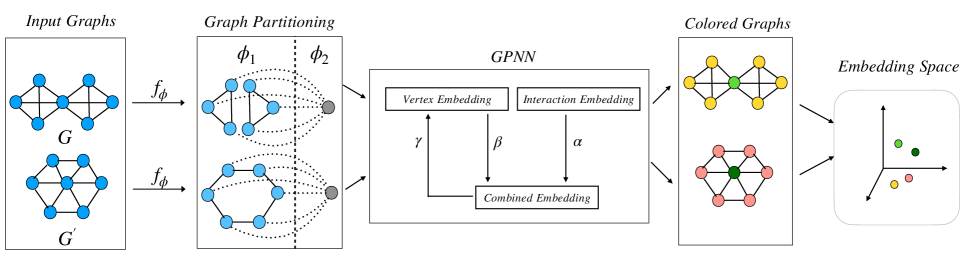
Figure 3: $G$ and $G^{{}^{\prime}}$ is a pair of graphs that cannot be distinguished by 1-WL. $f_{\phi}$ partitions these input graphs into two partitions denoted by $\phi_{1}$, and $\phi_{2}$. The intra-edges are marked using dotted lines. GPNN generates vertex representations taking interactions within and between partitions into account, making GPNN capable of distinguishing these two graphs.

Proposed GNN Architecture

We propose a novel GNN model, Graph Partitioning Neural Networks (GPNN), which integrates structural interactions into representation learning through graph partitioning.

Definition 7 (Partition colouring).

Let $C=C_{V}\cup C_{E}$ be a set of colors, where $C_{V}\cap C_{E}=\emptyset$, and $\{S_{1},\dots,S_{k}\}$ be a set of subgraphs generated by a graph partitioning scheme over $G$. A partition colouring $\lambda=(\lambda_{V},\lambda_{E})$ consists of the following:

• Vertex colouring: Each vertex $v\in V(G)$ is assigned a vertex color, defined as $\lambda_{V}:V(G)\rightarrow C_{V}$ such that $\lambda_{V}(v)=\lambda_{V}(u)$ if and only if $v\in V(S_{i})$ and $u\in V(S_{i})$.

• Edge colouring: Each pair of vertices $\{v,u\}\subseteq V(G)$ is assigned an edge color, defined as $\lambda_{E}:V(G)\times V(G)\rightarrow C_{E}$ such that

  $$\begin{array}[]{l}\lambda_{E}(v,u)=\\ \begin{cases}(\lambda_{V}(v),c_{\text{inter}},\lambda_{V}(u))&(v,u)\in E(G),\lambda_{V}(v)=\lambda_{V}(u);\\ (\lambda_{V}(v),c_{\text{intra}},\lambda_{V}(u))&(v,u)\in E(G),\lambda_{V}(v)\neq\lambda_{V}(u);\\ (\lambda_{V}(v),c_{\text{none}},\lambda_{V}(u))&(v,u)\notin E(G).\\ \end{cases}\end{array}$$

Each edge $(v,u)\in E(G)$ is classified as either an inter-edge if $\lambda_{V}(v)=\lambda_{V}(u)$ or an intra-edge if $\lambda_{V}(v)\neq\lambda_{V}(u)$. This leads to three edge colors $\{c_{\text{inter}},c_{\text{intra}},c_{\text{none}}\}$ in $\lambda_{E}$. Intuitively, inter-edges indicate interactions between vertices within one subgraph while intra-edges indicate interactions between vertices across different subgraphs.

Definition 8 (Coloured neighbourhood).

For each vertex $v\in V$, the neighbourhood $N(v)$ consists of a set of neighbouring vertex subsets $\{N^{1}(v),\dots,N^{k}(v)\}$, each of which is coloured with a distinct colour under $\lambda_{V}$ such that, for any two vertices $\{u,w\}\subseteq N(v)$, $\lambda_{V}(u)=\lambda_{V}(w)$ if and only if $\{u,w\}\subseteq N^{j}(v)$ for exactly one $j\in[1,k]$.

Let $\textsc{Upd}(.)$, $\textsc{Agg}(.)$, and $\textsc{Cmb}(.)$ be injective and permutation-invariant functions. Suppose that $\beta_{v}^{(0)}=\lambda_{V}(v)$ and $\gamma_{v}^{(0)}=\lambda_{V}(v)$ for any $v\in V(G)$. We embed the representations of each vertex $v$ with its neighbouring vertices into a continuous space, represented by $\beta_{v}^{(\ell+1)}$ at the $(\ell+1)$-th iteration as,

$$\beta_{v}^{(l+1)}=\textsc{Upd}\left(\gamma_{v}^{(l)},\textsc{Agg}\{\!\!\{\gamma_{u}^{(l)}|u\in N(v)\}\!\!\}\right)$$ (1)

Let $\alpha^{(0)}_{vu}=\lambda_{E}(v,u)$ for any $v,u\in V(G)$. We define the interaction embedding $\alpha^{(\ell+1)}_{vu}$ as the embedding of $(v,u)$ at the $(\ell+1)$-th iteration,

$$\alpha^{(\ell+1)}_{vu}= \textsc{Upd}\Bigl{(}\alpha_{vu}^{(\ell)},$$

$$\textsc{Agg}\Bigl{(}\{\!\!\{(\alpha_{vw}^{(\ell)},\alpha_{uw}^{(\ell)})|w\in N(v)\}\!\!\}\Bigr{)}\Bigr{)}$$ (2)

Here, $(v,u)$ may correspond to an inter-edge, an intra-edge, or a non-edge, depending on how $v$ and $u$ are connected in $G$ and partitioned by $f_{\Phi}$.

Then, we aggregate embeddings of neighboring vertices and their corresponding interactions from distinct graph partitions and combine these partition-wise embeddings into a combined embedding $\gamma_{v}$ as follows.

$$\gamma_{v}^{(\ell+1)}=\textsc{Cmb}\Bigl{(}\textsc{Agg}\left(\{\!\!\{(\beta_{u}^{(\ell+1)},\alpha_{vu}^{(\ell+1)})|u\in N_{d}^{1}(v)\}\!\!\}\right),\dots{\\ }\textsc{Agg}\left(\{\!\!\{(\beta_{u}^{(\ell+1)},\alpha_{vu}^{(\ell+1)})|u\in N_{d}^{k}(v)\}\!\!\}\right)\Bigr{)}$$ (3)

Finally, our model can be integrated as a plugin with any existing GNN models, which enhances these existing models with additional representation power for structural interactions. Let $h_{v}^{gnn}$ be a vertex embedding given by existing GNN model such as GIN (Xu et al. 2018), GCN (Kipf and Welling 2016), etc. We combine $\gamma_{v}^{(\ell+1)}$ with $h_{v}^{gnn}$ to obtain the final representation for each vertex $v$ as follows:

$$h_{v}= \textsc{Cmb}\left(h_{v}^{gnn},\gamma_{v}^{(\ell+1)}\right).$$ (4)

Figure 3 provides a high-level overview on the architecture of the proposed GNN model.

Theoretical Analysis

In this section, we conduct theoretical analysis on the expressivity and complexity of the proposed model GPNN.

Expressivity analysis

We discuss the expressivity of GPNN from two aspects: (1) How does a partition colouring determined by a chosen graph partition scheme affect the expressivity of GPNN? (2) How do different types of interactions affect the expressivity of GPNN?

Given two partition colourings $\lambda_{1}$ and $\lambda_{2}$, we say that $\lambda_{1}$ is more expressive than $\lambda_{2}$, denoted as $\lambda_{1}\succeq\lambda_{2}$, if and only if, for any two graphs $\{G,H\}\subseteq\mathcal{G}$, $G\equiv_{\lambda_{2}}H$ whenever $G\equiv_{\lambda_{1}}H$. This can be generalised to $k$-WL and GPNN, i.e., $M_{1}\succeq M_{2}$ means that $M_{1}$ is more expressive than $M_{2}$. A partition colouring $\lambda$ is trivial, denoted as $\lambda_{\bot}$, if $f_{\Phi}(G)=G$ for any $G\in\mathcal{G}$ and a partition colouring $\lambda$ is complete, denoted as $\lambda_{\top}$, if $f_{\Phi}(G)=f_{\Phi}(H)$ if and only if $G\simeq H$ for any $\{G,H\}\subseteq\mathcal{G}$.

For clarity, we use $\lambda$-GPNN^δ to refer to variants of GPNN, augmented by a partition colouring $\lambda$ and an interaction type $\delta\in\{\star,\diamond,\dagger\}$, where $\star$, $\diamond$, and $\dagger$ denote interactions of intra-edges ($E^{\star}$), interactions of intra-edges and inter-edges ($E^{\diamond}$), and all interactions including edges and non-edges ($E^{\dagger}$), respectively.

The following theorem states that the expressive power of $\lambda$-GPNN^δ is upper bounded by 3-WL when the partitioning scheme $\lambda$ is trivial and has expressive power less than 3-WL.

Theorem 2.

When $\lambda$ is trivial, the following hold:

• $\lambda$-GPNN${}^{\star}\equiv 1\text{-}WL$;

• $\lambda$-GPNN${}^{\star}\prec\lambda$-GPNN${}^{\diamond}\prec\lambda$-GPNN^†;

• $\lambda$-GPNN${}^{\dagger}\preceq 3\text{-}WL$.

We present the following theorem that states any variant of GPNN can be more expressive than 1-WL when the graph partitioning scheme is non-trivial.

Theorem 3.

When $\lambda$ is non-trivial, $\lambda\text{-GPNN}^{\delta}$ is strictly more expressive than 1-WL for any $\delta\in\{\star,\diamond,\dagger\}$.

Furthermore, we can see that for any two partition colorings, their corresponding GPNN^δ models always preserve the expressivity order of their respective partition colorings.

Theorem 4.

Let $\lambda_{1}$ and $\lambda_{2}$ be two partition colourings, and $\lambda_{1}\succeq\lambda_{2}$. Then $\lambda_{1}$-GPNN^δ $\succeq$ $\lambda_{2}$-GPNN^δ.

The following lemma states that, no matter which types of interactions are considered, the expressive power of $\lambda$-GPNN^δ is always at least as strong as its corresponding partition colouring $\lambda$.

Lemma 1.

$\lambda\text{-GPNN}^{\delta}\succeq\lambda$ for any $\lambda$ and any $\delta\in\{\star,\diamond,\dagger\}$.

Below we show that, for a fixed partition colouring $\lambda$ below 3-WL, the expressive power of $\lambda$-GPNN^δ strictly increases when more interactions are captured into representations. However, when a partition colouring $\lambda$ is strong as 3-WL, the expressive power of $\lambda$-GPNN^δ remains unchanged under different types of interactions.

Lemma 2.

When $\lambda\prec 3\text{-}WL$, the following holds:

$$\lambda\text{-GPNN}^{\dagger}\succ\lambda\text{-GPNN}^{\diamond}\succ\lambda\text{-GPNN}^{\star}.$$ (5)

Lemma 3.

When $\lambda\succeq 3\text{-}WL$, the following holds:

$$\lambda\text{-GPNN}^{\dagger}\equiv\lambda\text{-GPNN}^{\diamond}\equiv\lambda\text{-GPNN}^{\star}.$$ (6)

Theorem 5 can easily follow from Lemmas 1, 2, and 3.

Theorem 5.

For any partition colouring $\lambda$,

$$\lambda\text{-GPNN}^{\dagger}\succeq\lambda\text{-GPNN}^{\diamond}\succeq\lambda\text{-GPNN}^{\star}\succeq\lambda.$$ (7)

Details of the proofs for the above lemmas and theorems are included in the supplementary material.

Remark.  In a nutshell, GPNN obtains additional expressive power from two sources: the capacity of graph partitioning to separate structural components of different properties and the ability of capturing different types of structure interactions. For the former source, it relates to a spectrum of possible partition colourings which may range from a trivial colouring $\lambda_{\bot}$ (i.e., all nodes are assigned the same colour) to a complete colouring $\lambda_{\top}$ (i.e., orbit colouring (McKay and Piperno 2014)). The power of a chosen partition colouring sets the lower bound of GPNN in its ability to distinguish non-isomorphic graphs. For the latter source, GPNN is designed to tackle partition isomorphism and interaction isomorphism by considering different types of edges. Structural interactions corresponding to vertices within graph partitions enable GPNN to capture partition isomorphism, while structural interactions corresponding to vertices across graph partitions help capture interaction isomorphism. Nonetheless, the model capacity of GPNN alone is upper-bounded by 3-WL.

Complexity analysis

3-WL test has $O(|V|^{3})$ space complexity and $O(|E|^{2})$ time complexity (Hu et al. 2022). Our proposed models GPNN^⋆, GPNN^⋄, and GPNN^† have $O(|E^{\star}|^{2})$, $O(|E^{\diamond}|^{2})$, and $O(|E^{\dagger}|^{2})$ time complexities, respectively. Further, GPNN^⋆ and GPNN^⋄ usually require less time and space computational resources since $|E^{\star}|<\!\!<|E|$ and $|E^{\diamond}|<\!\!<|E|$ for real-world graphs. Therefore, GPNN^⋆ and GPNN^⋄ variants can often perform much more efficiently than the 3-WL algorithm.

A graph partitioning scheme used by GPNN should be computationally efficient, i.e., in linear or polynomial time in terms of the size of an input graph. Graph partitions are processed as a preprocessing step. In our experiments, we use a graph partitioning scheme which has time and space complexity of $O(|E|)$ (will be discussed in the next section).

Practical Choices of Graph Partitioning Schemes

In this section, we address the question of graph partitioning: how to define subgraphs and their interactions via a permutation-invariant graph partition scheme? In practice, there are many design choices available. Nonetheless, two important criteria permutation invariance and computational efficiency have to be fulfilled.

Below, we consider a graph partitioning scheme that is both permutation invariant and computationally efficient.

Definition 9 ($k$-Core property).

A subgraph $S$ has the $k$-core property on a graph $G$, called $k$-core subgraph of $G$, if $S$ is the largest induced subgraph of $G$ satisfying: $\forall v\in V(S)\hskip 5.69046pt\textsc{Deg}_{S}(v)\geq k$.

Let $\varphi_{j}$ denote the $j$-core property. Suppose that $\Phi_{core}=\{\phi_{j}\}_{j\in[1,k]}$ where $\phi_{j}=\varphi_{j}\wedge\neg\varphi_{j+1}$ defined as satisfying the $j$-core property but not the $j\text{+}1$-core property. Then the graph partitioning scheme $f_{\Phi_{core}}$ corresponds to the shell decomposition (Alvarez-Hamelin et al. 2005), which decomposes a graph $G$ into subgraphs, namely shells, each containing all the vertices belonging to the $j$-core subgraph but not the $j\text{+}1$-core subgraph.

$\Phi_{core}$ can be further refined as long as the refined graph properties are permutation invariant. Let $\phi\circ\psi$ denote the sequential composition of two properties $\phi$ and $\psi$ such that $(G,S_{j})\models\phi\circ\psi$ whenever $(G,S_{i})\models\phi$ and $(S_{i},S_{j})\models\psi$. We may have the following refined instances of $\Phi_{core}$:

• $\Phi_{core\text{-}degree}=\{\phi^{\prime}_{j}\}_{j\in[1,2k]}$ where $\phi^{\prime}_{2j-1}=\phi_{j}\circ\psi_{j}$, $\phi^{\prime}_{2j}=\phi_{j}\circ\neg\psi_{j}$, and $\psi_{j}=\forall v\in V(S_{j})\hskip 5.69046pt\textsc{Deg}_{S_{j}}(v)=j$.

• $\Phi_{core\text{-}onion}=\{\phi^{\prime}_{ji}\}_{j\in[1,k]}$ where $\phi^{\prime}_{ji}=\phi_{j}\circ\psi^{1}_{j}\circ,\dots,\circ\psi^{i}_{j}$, and $\psi_{j}^{i}$ refers to the $i$-th iteration to remove vertices with the lowest degree in the $j$-core subgraph.

One question may then arise as to how a partition colouring $\lambda$ determined by such $f_{\Phi}$ relate to $k$-WL? To answer this question, below we introduce the notion of $\lambda$-Equivalence.

Definition 10 ($\lambda$-Equivalence).

Let $\lambda=(\lambda_{V},\lambda_{E})$ be a partition colouring. Two graphs $G$ and $H$ are $\lambda$-equivalent, denoted as $G\equiv_{\lambda}H$, if they are indistinguishable by $\lambda$, i.e.,

• for each $c\in C_{V}$, $|\{v\in V(G)|\lambda_{V}(v)=c\}|$ = $|\{v^{\prime}\in V(H)|\lambda_{V}(v^{\prime})=c\}|$;

• for each $c\in C_{E}$, $|\{v,u\}\subseteq V(G)|\lambda_{E}(v,u)=c\}|$ = $|\{\{v^{\prime},u^{\prime}\}\subseteq V(H)|\lambda_{E}(v^{\prime},u^{\prime})=c\}|$.

Let $G\equiv_{\text{1-WL}}H$ denote that two graphs $G$ and $H$ are indistinguishable by applying $1$-WL. The following theorem states that the expressive power of the partition colourings based on the aforementioned $k$-core property and its extensions are indeed upper bounded by 1-WL. A detailed proof is included in the supplementary material.

Theorem 6.

Let $\lambda$ be a partition colouring based on $f_{\Phi}$ where $\Phi=\Phi_{core}$. Then $G\equiv_{\lambda}H$ whenever $G\equiv_{\text{1-WL}}H$.

Experiments

We conduct experiments to validate our theoretical results and evaluate the performance of GPNN. We aim to answer the following questions: (1) How well can GPNN empirically perform for graph classification, vertex classification, and graph regression tasks? (2) How do different types of interactions contribute to GPNN’s overall performance? (3) How effectively can different graph partitioning schemes perform on the learning of structural interactions of GPNN?

Benchmark datasets

We evaluate our model on three tasks; graph classification, graph regression, and vertex classification. For graph classification, we use small-scale real-world datasets and large-scale molecular datasets. These small-scale real-world datasets are from TU Datasets (Morris et al. 2020) that are related to the fields of molecular science, and bioinformatics. For large-scale molecular datasets, we select three molecuar datasets from Open Graph Benchmark (OGB) (Hu et al. 2020) namely, ogbg-moltoxcast, ogbg-moltox21, and ogbg-molhiv. Under graph regression task, we evaluate ZINC dataset (Dwivedi et al. 2023) and use a 12K subset of ZINC(250K) dataset (Irwin et al. 2012). Further, we use two homophilic datasets (Cora and Citeseer) (Sen et al. 2008) and three heterophilic datasets (Wisconsin, Texas, and Cornell) (Craven et al. 2000) to evaluate vertex classification.

Experimental setups

For TU datasets, we use 10-fold cross-validation, and report accuracy and standard deviation. We use the evaluation settings provided in Xu et al. (2018), and Feng et al. (2022). In the first setting, we average the test accuracy among all 10 folds and report a single epoch with the best mean accuracy and the standard deviation. In the second setting, we report the mean values for best accuracy and standard deviation for all test folds. For baselines, we selected GNN architectures that has expressive power similar to or beyond 1-WL. We use GIN (Xu et al. 2018), GraphSNN (Wijesinghe and Wang 2022), GIN-AK+ (Zhao et al. 2021), and KP-GIN (Feng et al. 2022) as baselines. For OGB datasets, we follow the experimental setup of Hu et al. (2020). We use GIN (Xu et al. 2018), GraphSNN (Wijesinghe and Wang 2022), GSN (Bouritsas et al. 2022), PNA (Corso et al. 2020), and CIN (Bodnar et al. 2021) as baselines.

For ZINC dataset, we follow the experimental setup described by Dwivedi et al. (2023) and compare our model with GIN (Xu et al. 2018), GCN (Kipf and Welling 2016), PPGN (Maron et al. 2019a), PNA (Corso et al. 2020), DGN (Beaini et al. 2021), and Deep LRP (Chen et al. 2020), and CIN (Bodnar et al. 2021) as baselines.

We follow a setup similar to Pei et al. (2020) for vertex classification, where we randomly split the vertices in the datasets into 60%, 20%, and 20% for training, validation, and testing, respectively. We take GIN (Xu et al. 2018), GCN (Kipf and Welling 2016), GAT (Velickovic et al. 2018), and GraphSAGE (Hamilton, Ying, and Leskovec 2017) as the base models and study their performance changes when incorporating GPNN variants for enhanced expressiveness.

Graph Partitioning Scheme

We use $\Phi_{core\text{-}degree}$ for our experiments. The reasons are two-fold; (1) Compared to $\Phi_{core}$, $\Phi_{core\text{-}degree}$ generates more structural components that exhibit different properties, yielding more useful insights on interactions among vertex subsets. (2) Compared to $\Phi_{core\text{-}onion}$, $\Phi_{core\text{-}degree}$ generates a reasonable number of graph partitions that help to maintain reasonable computational complexity in GPNN.

Hyper-parameters

We search for hyper-parameters of GPNN in the following ranges: number of layers $\in\{1,2,3,4,5\}$, $d$ $\in\{1,2,3,4,5\}$, dropout $\in\{0.0,0.1,0.2,0.5,0.6\}$, learning rate $\in\{0.009,0.01\}$, batch size $\in\{32,64,128\}$, hidden units $\in\{32,64,100\}$, and number of epochs $\in\{100,200,300,500\}$. We use Adam algorithm (Kingma 2015) as our optimizer. For ZINC and OGB datasets, initial learning rate decays with a factor of 0.5 after every 10 epochs. We do not use any learning rate decay technique for TU datasets.

In the appendix, we provide a summary of the statistics of datasets used in our experiments, as well as additional experimental results for graph regression, vertex classification, and ablation studies. These results further empirically analyze how well different graph partitioning schemes may affect the structural interaction learning in GPNNs on real-world datasets.

Results and Discussion

In this section we discuss the results of our experiments.

Graph Classification

TU Datasets

Table 1 reports the results on small-scale datasets in graph classification task. We can see that both GPNN^⋆ and GPNN^† models surpass existing baselines in both evaluation settings. GPNN significantly outperforms state-of-the-art methods under Setting 2 on datasets like PROTEINS and BZR. The performance of GPNN^⋆ also shows that interactions from intra-edges may carry new and useful information, contributing to graph classification on real-world datasets. As intra-edges are usually a small subset of all edges in a graph, GPNN^⋆ enables an efficient yet expressive solution for many graph classification tasks.

Experimental Setups	Methods	MUTAG	PTC-MR	PROTEINS	BZR	COX2
Setting 1 (Xu et al. 2018)	GIN	89.4 ± 5.6	64.6 ± 7.0	75.9 ± 2.8	85.6 ± 2.0	82.44 ± 3.0
	GraphSNN	91.24 ± 2.5	66.96 ± 3.5	76.51 ± 2.5	88.69 ± 3.2	82.86 ± 3.1
	GIN-AK+	91.30 ± 7.0	68.20 ± 5.6	77.10 ± 5.7	-	-
	KP-GIN	92.2 ± 6.5	66.8 ± 6.8	75.8 ± 4.6	-	-
	GPNN⋆	91.02 ± 7.1	66.20 ± 11.2	77.18 ± 4.6	88.60 ± 4.6	82.88 ± 4.6
	GPNN⋄	92.60 ± 4.8	65.95 ± 8.5	76.82 ± 3.9	89.12 ± 2.3	83.09 ± 3.1
Setting 2 (Feng et al. 2022)	GIN	92.8 ± 5.9	65.6 ± 6.5	78.8 ± 4.1	91.05 ± 3.4	88.87 ± 2.3
	GraphSNN	94.70 ± 1.9	70.58 ± 3.1	78.42 ± 2.7	91.12 ± 3.0	86.28 ± 3.3
	GIN-AK+	95.0 ± 6.1	74.1 ± 5.9	78.9 ± 5.4	-	-
	KP-GIN	95.6 ± 4.4	76.2 ± 4.5	79.5 ± 4.4	-	-
	GPNN⋆	97.89 ± 2.6	78.17 ± 6.2	81.40 ± 3.5	94.05 ± 2.6	89.09 ± 3.3
	GPNN⋄	97.37 ± 4.9	79.61 ± 7.3	85.53 ± 6.2	91.84 ± 1.6	89.72 ± 2.3

Table 1: Graph classification accuracy (%) ± standard deviation (%) for TU datasets. Under each setting, best results are highlighted in black and second best results are highlighted in blue. The results of baselines for MUTAG, PTC_MR and PROTEINS datasets are taken from Feng et al. (2022). The results of BZR and COX2 datasets are taken from Wijesinghe and Wang (2022), and You et al. (2021). For any baseline that is not reported in these papers, we use all settings the same as GPNN and report the results.

OGB Datasets

Table 2 reports the results on large-scale molecular datasets. Both variants of our model show comparable performance with other baselines. Additional structural information captured by GPNN adds more expressive power to the model that surpasses the performance of GIN which is known to have equivalent expressive power of 1-WL. Some baselines like CIN and GSN embed explicit structural information like cycle counts into node features in the learning process, which are known to have high correlations with molecular classes and features. In order to maintain generalizability, GPNN does not process any such hand selected domain-specific structural information.

Methods	ogbg- molhiv	ogbg- moltoxcast	ogbg- moltox21
GIN	75.58 ± 1.40	63.41 ± 0.74	74.91 ± 0.51
GraphSNN	78.51 ± 1.70	65.40 ± 0.71	75.45 ± 1.10
PNA	79.05 ± 1.30	-	-
GSN#	77.99 ± 1.00	-	-
CIN#	80.94 ± 0.57	-	-
GPNN⋆	78.12 ± 1.91	64.70 ± 0.44	76.13 ± 0.68
GPNN⋄	77.70 ± 2.23	64.48 ± 0.45	75.98 ± 0.39

Table 2: Graph classification ROC (%) ± standard deviation (%) for OGB datasets. Best results are highlighted in black and second best results are highlighted in blue. Results of GIN and GraphSNN are taken from Wijesinghe and Wang (2022). For other baseline results, we refer to Bodnar et al. (2021). The methods marked by # are based on pre-selected domain-specific structural information.

Ablation Studies

We perform an ablation study to understand how partitioning schemes may affect the performance of GPNN. We denote GPNN variants with a trivial graph partitioning scheme as $\lambda_{\bot}$-GPNN^δ and with the graph partitioning scheme $\Phi_{core\text{-}degree}$ as $\lambda_{core\text{-}degree}$-GPNN^δ, respectively. We use two datasets from TU repository (Morris et al. 2020) for the evaluation alongside the setup introduced by Feng et al. (2022). Results are reported in Table 3.

Methods	DHFR	PTC_FM
GIN	80.04 ± 4.9	70.50 ± 4.7
$\lambda_{\bot}$-GPNN⋆	80.03 ± 4.0	70.78 ± 4.1
$\lambda_{\bot}$-GPNN⋄	80.30 ± 3.0	71.34 ± 4.6
$\lambda_{\bot}$-GPNN†	78.97 ± 4.0	73.15 ± 3.7
$\lambda_{core\text{-}degree}$-GPNN⋆	82.01 ± 2.3	73.92 ± 6.0
$\lambda_{core\text{-}degree}$-GPNN⋄	82.15 ± 2.9	73.92 ± 4.9
$\lambda_{core\text{-}degree}$-GPNN†	80.16 ± 2.6	74.50 ± 5.8

Table 3: Ablation study accuracy (%) ± standard deviation (%) for DHFR and PTC_FM datasets.

From the results, we can see that GPNNs using $\Phi_{core\text{-}degree}$ perform better than ones using a trivial partitioning scheme. $\lambda_{\bot}$-GPNN^⋆ has similar results to GIN, which provides empirical evidence about its expressive power being aligned with Theorem 2. Further, when the partitioning scheme is $\Phi_{core\text{-}degree}$, GPNNs show considerable improvements over GIN. This empirically validates Theorem 3. Furthermore, $\lambda_{\bot}$-GPNN^† and $\lambda_{core\text{-}degree}$-GPNN^† achieve the highest improvement for PTC_FM dataset, which is consistent with their theoretical expressive powers. However, this does not hold true for DHFR dataset as GPNN^† variants show lower performance. We believe that this happens due to the higher computational complexity and large learnable parameter space introduced by GPNN^† variants that could hamper the training process on that dataset.

Conclusion

In this work we propose a novel perspective to tackle the graph isomorphism problem through the lens of graph partitioning. We introduce the notion of permutation-invariant graph partitioning to explore complex interactions among structural components and their vertex subsets that have common characteristics in graphs. Such interactions cannot be captured by existing GNN models efficiently and effectively. We further conduct a theoretical analysis on how structural interactions can enhance the expressive power of GNN models and their connections to k-WL hierarchy. Based on these, we introduce a GNN architecture, Graph Partitioning Neural Network (GPNN), that enables to integrate structural interactions revealed by graph partitioning into graph representation learning. We conduct experiments for graph benchmark datasets, and our empirical results validates the effectiveness of the proposed model.

Appendix

A. Model Architecture

In this section we describe the implementation details of GPNN. Let $\beta_{v}^{(0)}=\lambda_{V}(v)$, $\gamma_{v}^{(0)}=\lambda_{V}(v)$ and $\alpha_{vu}^{(0)}=\lambda_{E}(v,u)$. Equations 1 and Proposed GNN Architecture for the vertex and interaction embeddings are implemented as follows:

$$\beta_{v}^{(\ell+1)}=\textsc{Mlp}^{(\ell+1)}_{\theta}\Biggl{(}\left(1+\epsilon^{(\ell+1)}\right)\gamma_{v}^{(\ell)}+\sum_{u\in N(v)}\gamma_{u}^{(\ell)}\Biggr{)};$$ (8)

$$\alpha_{vu}^{(\ell+1)}=\textsc{Mlp}_{\psi}\Biggl{(}\left(1+\mu^{(\ell+1)}\right)\alpha_{vu}^{(\ell)}\\ +\sum_{w\in N(v)}\left(\alpha_{(vw)}^{(\ell)}+\alpha_{(vw)}^{(\ell)}\right)\Biggr{)}.$$ (9)

Here, $\beta_{v}^{(\ell+1)}\in\mathbb{R}^{d}$ is a vertex embedding; $\alpha_{vu}^{(\ell+1)}\in\mathbb{R}^{d}$ is an interaction embedding; $\gamma_{v}^{(\ell+1)}\in\mathbb{R}^{d}$ is an embedding that combines vertex embeddings and the corresponding interaction embeddings from the coloured neighbourhood of vertex $v$; $\mu^{(\ell+1)}$ and $\epsilon^{(\ell+1)}$ are learnable scalar parameters; $\textsc{Mlp}_{\theta}^{(\ell+1)}(.)$ and $\textsc{Mlp}_{\psi}^{(\ell+1)}(.)$ are multi-layer perceptron (MLP) functions, parameterized by $\theta$ and $\psi$, respectively.

The embedding $\gamma^{(\ell+1)}_{v,j}$ for each $j\in[1,k]$ is calculated as,

$$\gamma^{(\ell+1)}_{v,j}=\omega_{j}\left(\sum_{u\in N^{j}(v)}\left(\beta^{(\ell+1)}_{u}||\alpha^{(\ell+1)}_{vu}||p_{j}\right)W_{j}\right).$$ (10)

The combined embedding w.r.t. the whole neighbourhood of vertex $v$ is defined as

$$\gamma^{(\ell+1)}_{v}=\left(\gamma^{(\ell+1)}_{v,1}+\dots+\gamma^{(\ell+1)}_{v,k}\right).$$ (11)

For any $j\in[1,k]$, $\gamma^{(\ell+1)}_{v,j}$ is the vertex embedding of $v$ learnt at the $(\ell+1)$-th iteration with respect to a neighbouring vertex subset $N^{j}(v)$; $p_{j}\in\mathbb{R}^{1\times k}$ is a one-hot vector in which values are all zero except one at the $j$-th position; $W_{j}\in\mathbb{R}^{(2d+k)\times d}$ is a learnable linear transformation matrix; $\omega_{j}$ is a learnable scalar parameter. It is worthy to note that $p_{j}$ is critical for preserving the injectivity of Equation 3 in GPNN.

When GPNN is used as a plug-in, $\gamma^{(\ell+1)}$ can be concatenated with the corresponding vertex embedding $h_{v}^{gnn}$ generated by a chosen GNN as follows:

$$h_{v}= \textsc{Concat}\left(h_{v}^{gnn},\gamma^{(\ell+1)}\right)$$ (12)

Finally, we append a feature vector related to the number of connected components, provided by the graph partitioning scheme, to $h_{v}$ to enhance the representations.

B. Proofs of Lemmas and Theorems

In this section we provide the proofs to the lemmas and theorems presented in Section “Theoretical Analysis”.

Without loss of generality, we assume that the functions $\textsc{Agg}(.),\textsc{Cmb}(.)$ and $\textsc{Upd}(.)$ used in GPNN are injective and there are also sufficiently many layers in GPNN.

See 1

Proof.

We first prove one direction of Statement (a). From the definition of graph isomorphism, we know that if $G\simeq G^{{}^{\prime}}$, then there is a bijective mapping $f:V(G)\rightarrow V(G^{\prime})$ such that for any $(u,v)\in E(G)$, $(f(u),f(v))\in E(G^{{}^{\prime}})$. According to the definition of partition isomorphism, we know that if $G\simeq_{partition}G^{\prime}$, then there exists a bijective mapping $g:f_{\Phi}(G)\rightarrow f_{\Phi}(G^{\prime})$ such that $g(S_{i})\simeq S^{\prime}_{i}$ for every $i\in[1,k]$. Thus, if $G\simeq G^{{}^{\prime}}$, we know that the same bijective mapping from graph isomorphism $f:V(S_{i})\rightarrow V(S_{i}^{{}^{\prime}})$ such that for any $(u,v)\in E(S_{i})$, $(f(u),f(v))\in E(S_{i}^{{}^{\prime}})$ for any $i\in[1,k]$. Then, we consider the partition graphs $S_{G}$ and $S_{G}^{{}^{\prime}}$. By the definition of interaction isomorphism, we know that there exists a bijective function $t:B(G)\rightarrow B(G^{\prime})$ such that $(v,u)\in E(S_{G})$ iff $(t(v),t(u))\in E(S_{G^{\prime}})$. This can also be satisfied by $f$ where $f:V(S_{G})\rightarrow V(S_{G^{\prime}})$ such that for any $(u,v)\in S_{G^{\prime}}$, $(f(u),f(v))\in S_{G^{\prime}}$. Therefore, the bijective mapping of graph isomorphism satisfies both conditions of interaction-isomorphism, i.e., if $G\simeq G^{{}^{\prime}}$, then $G\simeq_{interaction}G^{{}^{\prime}}$ as well. However, the converse direction of Statement (a) does not hold. The pair of graphs shown in Figure 2(a) is interaction-isomorphic, but not isomorphic.

The first direction of Statement (b) can easily follow from the definition of interaction-isomorphism. The converse do not hold, which can be proven by the pair of graphs shown in Figure 2(b). The proof is complete.

∎

Before proving the next theorem, we recall 2-FWL test (Weisfeiler and Leman 1968) which has been shown to be logically equivalent to 3-WL test (Maron et al. 2019a). 2-FWL test initially provides a color $C^{0}(v,u)$ for each pair of vertices $v,u\in V(G)$, defined as follows.

$$C^{0}(v,u)=\begin{cases}c_{self}&u=v\\ c_{edge}&(u,v)\in E(G)\\ c_{non-edge}&(u,v)\notin E(G)\\ \end{cases}$$

Here, $c_{self},c_{edge}$ and $c_{non-edge}$ are initial colours. Then the iterative coloring process of 2-FWL is defined by

$$C^{(i+1)}(v,u)=\sigma(C^{(i)}(v,u),\\ \{\!\!\{(C^{(i)}(v,w),C^{(i)}(u,w))|w\in V(G)\}\!\!\}).$$

Note that $\sigma(.)$ is an injective hashing function. The expressive power of 2-FWL is known to be strictly higher than 1-WL test and 2-WL test (Balcilar et al. 2021).

See 2

Proof.

We begin with proving the first statement. Since $\lambda$ is trivial, $E^{\star}=\emptyset$. There are thus no structural interactions being considered by GPNN^⋆. As all vertices in a graph are assigned with the same initial color by a trivial $\lambda$ and no structural interactions can be identified, GPNN^⋆ would have the expressive power of 1-WL that is provided by Equation 1. Therefore, $\lambda$-GPNN${}^{\star}\equiv$ 1-WL.

To prove the second statement, we consider two parts: (1) $\lambda$-GPNN${}^{\star}\prec\lambda$-GPNN^⋄, (2) $\lambda$-GPNN${}^{\diamond}\prec\lambda$-GPNN^†.

For (1), when $\lambda$ is trivial, $E^{\diamond}$ = $E(G)$. Therefore, GPNN^⋆ would consider a subset of interaction features. It is trivial to see that $\lambda$-GPNN${}^{\star}\preceq\lambda$-GPNN^⋄. To prove, $\lambda$-GPNN${}^{\star}\prec\lambda$-GPNN^⋄, there should exist two graphs that can be distinguished by $\lambda$-GPNN^⋄ but not by $\lambda$-GPNN^⋆. We provide such two pairs of graphs in Figure 2(b). When we consider $\Phi_{core}$ as the properties for the graph partitioning scheme, $\lambda$-GPNN^⋄ can distinguish these pair of graph, but $\lambda$-GPNN^⋆ fails to do so. This proves $\lambda$-GPNN${}^{\star}\prec\lambda$-GPNN^⋄. For (2), since $E^{\diamond}\subseteq E^{\dagger}$, we can say that $\lambda$-GPNN${}^{\diamond}\preceq\lambda$-GPNN^†. The pair of graphs in Figure 2(a) shows that there exist at least two graphs that can be distinguished by $\lambda$-GPNN^† but cannot be distinguished by $\lambda$-GPNN^⋄. These together constitute the proof of $\lambda$-GPNN${}^{\diamond}\prec\lambda$-GPNN^†.

Now we prove the third statement. Under the following conditions, GPNN has the expressive power equivalent to 3-WL test.

• Consider all interactions including edges and non-edges in the graph for $\alpha_{vu}$ in Equation Proposed GNN Architecture.

• $\forall v\in V(G)$, $N(v)$ = $V(G)$.

Since $N(v)\subseteq V(G)$ in GPNN, we can say that $\lambda$-GPNN${}^{\dagger}\preceq 3\text{-}WL$. ∎

See 3

Proof.

Regardless of $\lambda$, Equation Proposed GNN Architecture ensures that GPNN is at least as expressive as 1-WL (see Theorem 3 of Xu et al. (2018)). Therefore, $\lambda\text{-GPNN}^{\delta}\succeq\text{1-WL}$ for any non-trivial $\lambda$. Furthermore, we prove the strictness, i.e., $\lambda\text{-GPNN}^{\delta}\succ\text{1-WL}$, by presenting a pair of graphs that can be distinguished by GPNN^⋆, but not by 1-WL. Figure 3 provides such pair of graphs. Given $E^{*}\subseteq E^{\diamond}\subseteq E^{\dagger}$, this pair of graphs can also be distinguished by $\lambda\text{-GPNN}^{\diamond}$ and $\lambda\text{-GPNN}^{\dagger}$. Therefore, when $\lambda$ is non-trivial, $\lambda\text{-GPNN}^{\delta}\succ\text{1-WL}$. ∎

See 1

Proof.

GPNN receives its initial vertex coloring from $\lambda$. Then, the expressive power given by Equation  1 of GPNN is equivalent to the expressive power of $\lambda$ or 1-WL, whichever the higher. Thus, when not considering any structural interactions, the expressive power of GPNN is the same as the maximum expressive power of $\lambda$ and 1-WL. This would intrinsically make GPNN lower bounded by the expressive power of $\lambda$. Thus, we can derive that $\lambda$-GPNN^δ $\succeq\lambda$. ∎

See 4

Proof.

By the definition of $\lambda$-GPNN^δ, GPNN starts with a graph in which vertices are coloured by $\lambda$. Since $\lambda_{1}\succeq\lambda_{2}$, we know that, for any two vertices $\{v,u\}\subseteq V(G)$, if $v$ and $u$ are assigned with the same colour by $\lambda_{1}$, then they must be assigned with the same colour by $\lambda_{2}$; the converse does not necessarily hold. Then, by the definition of GPNN in terms of Equations 1, Proposed GNN Architecture, and 3, we know that if two vertices $\{v,u\}\subseteq V(G)$ are assigned with different colours by $\lambda$, then they would always have different colours after applying $\lambda$-GPNN^δ with any number of layers. That is, $\lambda$-GPNN^δ always refines a partitioning colouring $\lambda$. Since the same equations (Equations 1, Proposed GNN Architecture, and 3) are applied by $\lambda_{1}$-GPNN^δ and $\lambda_{2}$-GPNN^δ on vertices in $G$, which only differ in partitioning colourings, and also the functions $\textsc{Agg}(.),\textsc{Cmb}(.)$ and $\textsc{Upd}(.)$ used in GPNN are injective, any two vertices $v,u\in V(G)$ must have different colours by applying $\lambda_{1}$-GPNN^δ whenever they have different colours by applying $\lambda_{2}$-GPNN^δ, but not vice versa.

∎

See 2

Proof.

Since $E^{\star}\subseteq E^{\diamond}\subseteq E^{\dagger}$, we can derive the following: $\lambda$-GPNN^⋆ $\preceq$ $\lambda$-GPNN^⋄ $\preceq$ $\lambda$-GPNN^†. Now we need to show that $\lambda$-GPNN^⋆ $\prec$ $\lambda$-GPNN^⋄ and $\lambda$-GPNN^⋄ $\prec$ $\lambda$-GPNN^† hold. We know that $\Phi_{core}\prec\text{3-WL}$. When applying $f_{\Phi}$ with $\Phi=\Phi_{core}$, $\lambda$-GPNN^⋄ can distinguish the graph pair shown in Figure 2(b), but $\lambda$-GPNN^⋆ cannot. Similarly, $\lambda$-GPNN^† can distinguish the graph pair shown in Figure 2(a), but $\lambda$-GPNN^⋄ cannot. This proves the strictness in $\lambda$-GPNN^⋆ $\prec$ $\lambda$-GPNN^⋄ and $\lambda$-GPNN^⋄ $\prec$ $\lambda$-GPNN^†. Putting these things together, the lemma is proven. ∎

See 3

Proof.

The expressive power of GPNN by learning representations of structural interactions on top of node representations is upper bounded by 3-WL. When $\lambda\succeq\text{3-WL}$, Equations 1, Proposed GNN Architecture, and 3 in GPNN would not add any additional expressive power to distinguish nodes and graphs. Therefore, all GPNN variants would have same expressive power which is provided by the initial coloring of $\lambda$. irrespective of the types of structural interactions they consider. ∎

Datasets	Task Type	# Graphs	Avg #Nodes	Avg #Edges	# Classes
MUTAG	Graph Classification	188	17.93	19.79	2
PTC_MR	Graph Classification	344	14.29	14.69	2
PTC_FM	Graph Classification	349	14.11	14.48	2
BZR	Graph Classification	405	35.75	38.36	2
COX2	Graph Classification	467	41.22	43.45	2
ENZYMES	Graph Classification	600	32.63	62.14	6
DHFR	Graph Classification	756	42.43	44.54	2
PROTEINS	Graph Classification	1,113	39.06	72.82	2
ogbg-moltox21	Graph Classification	7,831	18.6	19.3	2
ogbg-moltoxcast	Graph Classification	8,576	18.8	19.3	2
ogbg-molhiv	Graph Classification	41,127	25.5	27.5	2
ZINC	Graph Regression	12,000	23.1	49.8	1

Table 4: Dataset Statistics for Graph Classification and Regression

Datasets	# Nodes	# Edges	# Features	# Classes
Cora	2708	5278	1433	7
CiteSeer	3327	4552	3703	6
Wisconsin	251	466	1703	5
Cornell	183	277	1703	5
Texas	183	279	1703	5

Table 5: Dataset Statistics for Vertex Classification

See 5

Proof.

By Lemmas 2 and 3, $\lambda$-GPNN^⋆ $\preceq$ $\lambda$-GPNN^⋄ $\preceq$ $\lambda$-GPNN^† holds. Further, by Lemma 1, $\lambda\preceq\lambda$-GPNN^⋆ holds. Thus, the above theorem is proven.

∎

See 6

Proof.

Let $\lambda_{1\text{-}WL}$ and $\lambda_{core}$ be two partition colourings generated by 1-WL and a core decomposition using the k-core property (Definition 9), respectively.

Then, we first prove that $\forall u,v\in V(G),\lambda_{core}(u)\neq\lambda_{core}(v)\implies\lambda_{\text{1-WL}}(u)\neq\lambda_{\text{1-WL}}(v)$. Core decomposition is an iterative peeling algorithm which, given an input graph $G$, starts the peeling process from vertices of the lowest degree in the left subgraph of $G$. If $\lambda_{core}(u)\neq\lambda_{core}(v)$, then the vertices $u$ and $v$ must appear in different peeling iterations; otherwise, they would have the same colour, i.e., $\lambda_{core}(u)=\lambda_{core}(v)$. Let $P_{u}$ and $P_{v}$ be two posets (partially ordered sets) that contain the set of all vertices being removed before $u$ and $v$ by the core decomposition algorithm, respectively. Here, we define that any two vertices $w$ and $w^{\prime}$ are ordered, i.e., $w<w^{\prime}$, if the vertex $w$ appears in an peeling iteration before the iteration where $w^{\prime}$ appears. As $u$ and $v$ appear in different peeling iterations, $P_{u}$ cannot be same as $P_{v}$. Thus, $P_{u}$ and $P_{v}$ should have different degree sequences. On the other hand, 1-WL algorithm achieves its stable coloring based on the neighborhood degree sequence of each node (Smith 2019). Given $P_{u}$ and $P_{v}$ are different, $\lambda_{\text{1-WL}}(u)$ and $\lambda_{\text{1-WL}}(v)$ must be different as well.

In the following, we further show that there exists at least one pair of graphs that can be distinguished by $\lambda_{\text{1-WL}}$, but not by $\lambda_{\text{core}}$.

Consider the graphs $G$ and $G^{\prime}$ depicted in Figure 4. When $\lambda_{\text{core}}$ is applied, all vertices in both $G$ and $G^{{}^{\prime}}$ would be assigned with the same color. However, when applying $\lambda_{\text{1-WL}}$, the vertices with degree 3 in $G$ would be assigned a color that is different from the color of the vertices with degree 2 in $G$. Furthermore, the vertices of degree 2 in $G$ would have a color that is different from the color of the vertices with degree 2 in $G^{{}^{\prime}}$. Therefore, these pair of graph can be distinguished by $\lambda_{\text{1-WL}}$, but not by $\lambda_{\text{core}}$.

Therefore, $\lambda_{1\text{-}WL}\succ\lambda_{core}$. Then, $G\equiv_{\lambda}H$ whenever $G\equiv_{\text{1-WL}}H$ holds. This completes the proof.

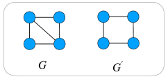
Figure 4: Two graphs that can be distinguished by their node colours from $\lambda_{\text{1-WL}}$, but not by their node colours from $\lambda_{\text{core}}$

.

∎

Methods	DHFR	ENZYMES	PTC_FM
GIN	80.04 ± 4.9	34.17 ± 4.2	70.50 ± 4.7
$\lambda_{\text{core}}$-GPNN⋆	80.43 ± 3.1	35.33 ± 2.9	74.48 ± 4.2
$\lambda_{\text{core}}$-GPNN⋄	80.56 ± 2.6	44.67 ± 5.6	72.48 ± 6.4
$\lambda_{\text{core-degree}}$-GPNN⋆	82.01 ± 2.3	38.50 ± 3.8	73.92 ± 6.0
$\lambda_{\text{core-degree}}$-GPNN⋄	82.15 ± 2.9	39.83 ± 4.1	73.92 ± 4.9
$\lambda_{\text{core-onion}}$-GPNN⋆	81.61 ± 2.4	36.50 ± 3.2	72.79 ± 6.4
$\lambda_{\text{core-onion}}$-GPNN⋄	82.14 ± 3.2	36.83 ± 3.2	73.36 ± 4.9
$\lambda_{\text{degree}}$-GPNN⋆	82.41 ± 3.7	35.50 ± 4.7	73.05 ± 3.5
$\lambda_{\text{degree}}$-GPNN⋄	82.41 ± 2.9	43.33 ± 4.8	73.19 ± 3.7
$\lambda_{\text{triangle}}$-GPNN⋆	79.37 ± 2.5	41.33 ± 3.0	70.48 ± 4.5
$\lambda_{\text{triangle}}$-GPNN⋄	80.96 ± 3.1	40.16 ± 3.5	71.92 ± 4.6

Table 6: Ablation study accuracy (%) ± standard deviation (%). Highest results from GPNN^⋆, and GPNN^⋄ are highlighted in black and blue, respectively.

Dataset	Partitioning	# Partitions	Avg	Avg	# Intra-Edges / # Inter-Edges
	Scheme		# Intra-Edges	# Inter-Edges
DHFR	$\Phi_{\text{core}}$	3	12.38	32.16	28 /  72
	$\Phi_{\text{core-degree}}$	5	21.79	22.75	49 /  51
	$\Phi_{\text{core-onion}}$	27	33.88	10.66	76 /  24
	$\Phi_{\text{degree}}$	7	34.72	9.82	78 /  22
	$\Phi_{\text{triangle}}$	1	0.00	44.54	0 /  100
ENZYMES	$\Phi_{\text{core}}$	5	2.59	59.55	4 /  96
	$\Phi_{\text{core-degree}}$	7	23.33	38.81	38 /  62
	$\Phi_{\text{core-onion}}$	22	44.78	17.36	72 /  28
	$\Phi_{\text{degree}}$	10	42.44	19.70	68 /  32
	$\Phi_{\text{triangle}}$	14	41.80	20.34	67 /  33
PTC_FM	$\Phi_{\text{core}}$	3	2.14	12.34	15 /  85
	$\Phi_{\text{core-degree}}$	5	4.70	9.78	32 /  68
	$\Phi_{\text{core-onion}}$	15	8.87	5.61	61 /  39
	$\Phi_{\text{degree}}$	5	9.55	4.93	66 /  34
	$\Phi_{\text{triangle}}$	2	0.05	14.43	1 /  99

Table 7: Statistics for five graph partitioning schemes used in ablation studies.

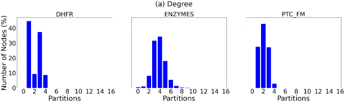
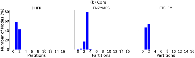
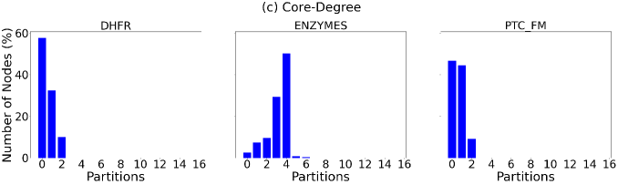
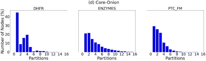
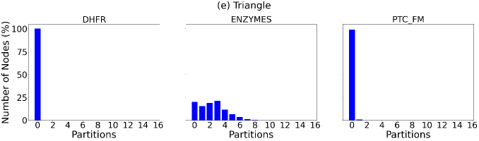
Figure 5: Node distributions concerning partitions under five graph partitioning schemes.

Methods	Cora	CiteSeer	Wisconsin	Texas	Cornell
GIN	80.6 ± 0.4	73.8 ± 0.4	70.5 ± 1.6	61.6 ± 1.1	28.9 ± 2.6
GPNN⋆GIN	82.0 ± 1.4	74.8 ± 0.3	71.3 ± 1.7	62.3 ± 1.9	69.4 ± 13.3
GPNN⋄GIN	82.3 ± 0.9	74.2 ± 0.4	71.4 ± 1.5	61.5 ± 1.5	67.2 ± 13.9
GCN	82.6 ± 1.5	78.1 ± 0.2	55.8 ± 19.5	53.1 ± 21.6	54.7 ± 21.9
GPNN⋆GCN	83.2 ± 1.5	78.8 ± 0.3	56.5 ± 17.7	51.8 ± 23.0	61.1 ± 18.9
GPNN⋄GCN	82.8 ± 1.7	78.6 ± 0.3	56.1 ± 18.2	57.7 ± 22.5	55.1 ± 21.3
GAT	83.9 ± 0.8	77.7 ± 0.6	58.6 ± 1.6	62.0 ± 2.2	64.5 ± 1.4
GPNN⋆GAT	84.2 ± 0.8	78.1 ± 0.6	60.3 ± 2.5	64.3 ± 3.1	66.0 ± 1.6
GPNN⋄GAT	84.5 ± 0.4	77.8 ± 0.8	59.9 ± 2.5	64.4 ± 3.4	65.3 ± 1.4
GraphSAGE	84.5 ± 0.3	77.9 ± 0.5	87.0 ± 1.7	81.6 ± 2.3	80.9 ± 1.9
GPNN⋆GraphSAGE	84.9 ± 0.3	78.2 ± 0.6	87.4 ± 1.2	79.5 ± 2.0	82.6 ± 1.9
GPNN⋄GraphSAGE	84.7 ± 0.5	78.1 ± 0.5	87.1 ± 1.6	82.0 ± 1.3	84.7 ± 1.9

Table 8: Vertex Classification Accuracy (%) averaged over 10 random splits. The best results are highlighted in black.

C. Dataset Statistics

In Table 4 and  5, we provide a summary of statistics for datasets that we have considered in all our experiments.

D. Additional Ablation Studies

Choosing a graph partitioning scheme is one of the key design decisions of GPNN. We perform an ablation study to understand how a graph partitioning scheme may affect the learning of structural interactions in GPNN.

We consider six graph partitioning schemes in this experiment: $\Phi_{\text{core}}$, $\Phi_{\text{core-degree}}$, $\Phi_{\text{core-onion}}$, $\Phi_{\text{degree}}$, and $\Phi_{\text{triangle}}$. Here, $\Phi_{\text{degree}}$ refers to the graph properties which partition vertices based on their degrees, while $\Phi_{triangle}$ refers to the graph properties which partition vertices based on the number of triangles which they participate in. We denote GPNN variants with these graph partitioning schemes as $\lambda_{\text{core}}$-GPNN, $\lambda_{\text{core-degree}}$-GPNN, $\lambda_{\text{core-onion}}$-GPNN, $\lambda_{\text{degree}}$-GPNN, and $\lambda_{\text{triangle}}$-GPNN, respectively.

We conduct experiments on three datasets from TU repository (Morris et al. 2020), following the setup used by Feng et al. (2022). The results are shown in Table 6. Apart from the results, we provide statistical information on these datasets under each graph partitioning scheme in Table 7. Furthermore, Figure 5 depicts the node distribution with respect to partitions in each graph partitioning scheme.

From the results in Table 6, we can see that GPNN^⋄ consistently outperforms GPNN^⋆ in almost every graph partitioning scheme. This is mainly due to the higher expressive power of GPNN^⋄ than GPNN^⋆ by considering structural interactions from both inter-edges and intra-edges. Further, it is notable that the performance of GPNN^⋆ becomes lower when the average number of intra-edges in a graph partitioning is less (and vice versa). For GPNN^⋆, this is expected as the model’s expressive power mainly relies on the strength of structural interactions from intra-edges.

When comparing the model performance under different graph partitioning schemes, $\Phi_{\text{core-degree}}$ and $\Phi_{\text{degree}}$ schemes show consistently better performance compared to the other schemes. We identify three main reasons for this. Firstly, these two schemes generate considerable amount of structural interactions from intra-edges as shown in Figure 5(a) and 5(c), which helps GPNN to learn the structural behaviour of a graph. Secondly, the number of graph partitions generated by these two schemes is sufficient but not excessive, thereby without adding any computational burden in the training process. In addition to these, the node distribution with respect to partitions in these schemes are close to normal distributions as shown in Figure 5(a) and 5(c). This could have a positive impact on model training as machine learning models are known to generally perform well with normally distributed data patterns. Even though $\Phi_{\text{core-onion}}$ also generates a considerable number of structural interactions from intra-edges as shown in Figure 5(d), the learning complexity that it generates by a large number of partitions can be attributed for its middling performance. $\Phi_{\text{triangle}}$ performs similar to GIN on DHFR and PTC_FM datasets as it generates few structural interactions from intra-edges on these datasets as shown in Figure 5(e). However, there are good performance gains on ENZYMES dataset by $\Phi_{\text{triangle}}$. We can see from Table 7 that this is because $\Phi_{\text{triangle}}$ generates substantial structural interactions from intra-edges, thereby leading to very good performance by GPNN^⋆ for ENZYMES dataset. We also identify another reason for this better performance. $\Phi_{\text{triangle}}$ can distinguish some graphs that cannot be distinguished by 1-WL. Therefore, even without any interactions, GPNN would be strictly powerful that 1-WL when we use $\Phi_{\text{triangle}}$ as the graph partitioning scheme. In such cases, GPNN would benefit more from $\Phi_{\text{triangle}}$ compared to other 1-WL upper-bounded graph partitioning schemes.

E. Additional Results for Graph Regression

We evaluate GPNN for Zinc 12K dataset without the consideration of edge features. We compare GPNN performance with other expressive GNNs that mainly focus on learning topological features. The results are summarized in table 9.

According to the results, both GPNN variants show competitive performance in the regression task. Differently from models like CIN , GPNN does not process any hand crafted domain-specific structural information that are known to be highly correlated to molecular prediction tasks. Therefore, our model performance is less than such models.

Methods	ZINC
GCN	0.459 ± 0.006
PPGN	0.407 ± 0.028
GIN	0.387 ± 0.015
PNA	0.320 ± 0.032
DGN	0.219 ± 0.010
Deep LRP#	0.223 ± 0.008
CIN#	0.115 ± 0.003
GPNN⋆	0.214 ± 0.018
GPNN⋄	0.222 ± 0.021

Table 9: Graph Regression MAE ± standard deviation for ZINC 12K dataset. The best results are highlighted in black and the second best results are highlighted in blue. For the baseline results, we refer to Bodnar et al. (2021). The methods marked by # are based on pre-selected domain-specific structural information.

F. Additional Results for Vertex Classification

Table 8 shows that GPNN can enhance the vertex classification performance of existing GNNs by incorporating structural interaction information.

References

- Abu-El-Haija et al. (2019) Abu-El-Haija, S.; Perozzi, B.; Kapoor, A.; Alipourfard, N.; Lerman, K.; Harutyunyan, H.; Ver Steeg, G.; and Galstyan, A. 2019. Mixhop: Higher-order graph convolutional architectures via sparsified neighborhood mixing. In international conference on machine learning, 21–29. PMLR.
- Alvarez-Hamelin et al. (2005) Alvarez-Hamelin, J.; Dall’Asta, L.; Barrat, A.; and Vespignani, A. 2005. Large scale networks fingerprinting and visualization using the k-core decomposition. Advances in neural information processing systems, 18.
- Balcilar et al. (2021) Balcilar, M.; Héroux, P.; Gauzere, B.; Vasseur, P.; Adam, S.; and Honeine, P. 2021. Breaking the limits of message passing graph neural networks. In International Conference on Machine Learning, 599–608. PMLR.
- Barceló et al. (2021) Barceló, P.; Geerts, F.; Reutter, J.; and Ryschkov, M. 2021. Graph neural networks with local graph parameters. Advances in Neural Information Processing Systems, 34: 25280–25293.
- Beaini et al. (2021) Beaini, D.; Passaro, S.; Létourneau, V.; Hamilton, W.; Corso, G.; and Liò, P. 2021. Directional graph networks. In International Conference on Machine Learning, 748–758. PMLR.
- Bevilacqua et al. (2021) Bevilacqua, B.; Frasca, F.; Lim, D.; Srinivasan, B.; Cai, C.; Balamurugan, G.; Bronstein, M. M.; and Maron, H. 2021. Equivariant subgraph aggregation networks. arXiv preprint arXiv:2110.02910.
- Bodnar et al. (2021) Bodnar, C.; Frasca, F.; Otter, N.; Wang, Y.; Lio, P.; Montufar, G. F.; and Bronstein, M. 2021. Weisfeiler and lehman go cellular: Cw networks. Advances in Neural Information Processing Systems, 34: 2625–2640.
- Bouritsas et al. (2022) Bouritsas, G.; Frasca, F.; Zafeiriou, S. P.; and Bronstein, M. 2022. Improving graph neural network expressivity via subgraph isomorphism counting. IEEE Transactions on Pattern Analysis and Machine Intelligence.
- Cai, Fürer, and Immerman (1992) Cai, J.-Y.; Fürer, M.; and Immerman, N. 1992. An optimal lower bound on the number of variables for graph identification. Combinatorica, 12(4): 389–410.
- Chen et al. (2020) Chen, Z.; Chen, L.; Villar, S.; and Bruna, J. 2020. Can graph neural networks count substructures? Advances in neural information processing systems, 33: 10383–10395.
- Chiang et al. (2019) Chiang, W.-L.; Liu, X.; Si, S.; Li, Y.; Bengio, S.; and Hsieh, C.-J. 2019. Cluster-gcn: An efficient algorithm for training deep and large graph convolutional networks. In Proceedings of the 25th ACM SIGKDD international conference on knowledge discovery & data mining, 257–266.
- Corso et al. (2020) Corso, G.; Cavalleri, L.; Beaini, D.; Liò, P.; and Veličković, P. 2020. Principal neighbourhood aggregation for graph nets. Advances in Neural Information Processing Systems, 33: 13260–13271.
- Cotta, Morris, and Ribeiro (2021) Cotta, L.; Morris, C.; and Ribeiro, B. 2021. Reconstruction for powerful graph representations. Advances in Neural Information Processing Systems, 34: 1713–1726.
- Craven et al. (2000) Craven, M.; DiPasquo, D.; Freitag, D.; McCallum, A.; Mitchell, T.; Nigam, K.; and Slattery, S. 2000. Learning to construct knowledge bases from the World Wide Web. Artificial intelligence, 118(1-2): 69–113.
- Dwivedi et al. (2023) Dwivedi, V. P.; Joshi, C. K.; Luu, A. T.; Laurent, T.; Bengio, Y.; and Bresson, X. 2023. Benchmarking Graph Neural Networks. Journal of Machine Learning Research, 24(43): 1–48.
- Feng et al. (2022) Feng, J.; Chen, Y.; Li, F.; Sarkar, A.; and Zhang, M. 2022. How powerful are k-hop message passing graph neural networks. arXiv preprint arXiv:2205.13328.
- Gaunt et al. (2018) Gaunt, A.; Tarlow, D.; Brockschmidt, M.; Urtasun, R.; Liao, R.; and Zemel, R. 2018. Graph Partition Neural Networks for Semi-Supervised Classification.
- Gilmer et al. (2017) Gilmer, J.; Schoenholz, S. S.; Riley, P. F.; Vinyals, O.; and Dahl, G. E. 2017. Neural message passing for quantum chemistry. In International conference on machine learning, 1263–1272. PMLR.
- Hamilton, Ying, and Leskovec (2017) Hamilton, W.; Ying, Z.; and Leskovec, J. 2017. Inductive representation learning on large graphs. Advances in neural information processing systems, 30.
- Horn et al. (2021) Horn, M.; De Brouwer, E.; Moor, M.; Moreau, Y.; Rieck, B.; and Borgwardt, K. 2021. Topological graph neural networks. arXiv preprint arXiv:2102.07835.
- Hu et al. (2020) Hu, W.; Fey, M.; Zitnik, M.; Dong, Y.; Ren, H.; Liu, B.; Catasta, M.; and Leskovec, J. 2020. Open graph benchmark: Datasets for machine learning on graphs. Advances in neural information processing systems, 33: 22118–22133.
- Hu et al. (2022) Hu, Y.; Wang, X.; Lin, Z.; Li, P.; and Zhang, M. 2022. Two-Dimensional Weisfeiler-Lehman Graph Neural Networks for Link Prediction.
- Huang et al. (2022) Huang, Y.; Peng, X.; Ma, J.; and Zhang, M. 2022. Boosting the Cycle Counting Power of Graph Neural Networks with I2-GNNs. arXiv preprint arXiv:2210.13978.
- Irwin et al. (2012) Irwin, J. J.; Sterling, T.; Mysinger, M. M.; Bolstad, E. S.; and Coleman, R. G. 2012. ZINC: a free tool to discover chemistry for biology. Journal of chemical information and modeling, 52(7): 1757–1768.
- Kiefer (2020) Kiefer, S. 2020. Power and limits of the Weisfeiler-Leman algorithm. Ph.D. thesis, Dissertation, RWTH Aachen University, 2020.
- Kingma (2015) Kingma, D. 2015. Adam: a method for stochastic optimization. In International Conference on Learning Representations (ICLR).
- Kipf and Welling (2016) Kipf, T. N.; and Welling, M. 2016. Semi-supervised classification with graph convolutional networks. arXiv preprint arXiv:1609.02907.
- Maron et al. (2019a) Maron, H.; Ben-Hamu, H.; Serviansky, H.; and Lipman, Y. 2019a. Provably powerful graph networks. Advances in neural information processing systems, 32.
- Maron et al. (2019b) Maron, H.; Fetaya, E.; Segol, N.; and Lipman, Y. 2019b. On the universality of invariant networks. In International conference on machine learning, 4363–4371. PMLR.
- McKay and Piperno (2014) McKay, B. D.; and Piperno, A. 2014. Practical graph isomorphism, II. Journal of symbolic computation, 60: 94–112.
- Miao et al. (2021) Miao, X.; Gürel, N. M.; Zhang, W.; Han, Z.; Li, B.; Min, W.; Rao, S. X.; Ren, H.; Shan, Y.; Shao, Y.; et al. 2021. Degnn: Improving graph neural networks with graph decomposition. In Proceedings of the 27th ACM SIGKDD Conference on Knowledge Discovery & Data Mining, 1223–1233.
- Morris et al. (2020) Morris, C.; Kriege, N. M.; Bause, F.; Kersting, K.; Mutzel, P.; and Neumann, M. 2020. Tudataset: A collection of benchmark datasets for learning with graphs. arXiv preprint arXiv:2007.08663.
- Morris, Rattan, and Mutzel (2020) Morris, C.; Rattan, G.; and Mutzel, P. 2020. Weisfeiler and Leman go sparse: Towards scalable higher-order graph embeddings. Advances in Neural Information Processing Systems, 33: 21824–21840.
- Morris et al. (2019) Morris, C.; Ritzert, M.; Fey, M.; Hamilton, W. L.; Lenssen, J. E.; Rattan, G.; and Grohe, M. 2019. Weisfeiler and leman go neural: Higher-order graph neural networks. In Proceedings of the AAAI conference on artificial intelligence, volume 33, 4602–4609.
- Mu et al. (2023) Mu, Z.; Tang, S.; Zong, C.; Yu, D.; and Zhuang, Y. 2023. Graph neural networks meet with distributed graph partitioners and reconciliations. Neurocomputing, 518: 408–417.
- Nikolentzos, Dasoulas, and Vazirgiannis (2020) Nikolentzos, G.; Dasoulas, G.; and Vazirgiannis, M. 2020. k-hop graph neural networks. Neural Networks, 130: 195–205.
- Pei et al. (2020) Pei, H.; Wei, B.; Chang, K. C.-C.; Lei, Y.; and Yang, B. 2020. Geom-gcn: Geometric graph convolutional networks. arXiv preprint arXiv:2002.05287.
- Sato (2020) Sato, R. 2020. A survey on the expressive power of graph neural networks. arXiv preprint arXiv:2003.04078.
- Sen et al. (2008) Sen, P.; Namata, G.; Bilgic, M.; Getoor, L.; Galligher, B.; and Eliassi-Rad, T. 2008. Collective classification in network data. AI magazine, 29(3): 93–93.
- Smith (2019) Smith, K. M. 2019. On neighbourhood degree sequences of complex networks. Scientific reports, 9(1): 8340.
- Velickovic et al. (2018) Velickovic, P.; Cucurull, G.; Casanova, A.; Romero, A.; Lio, P.; and Bengio, Y. 2018. Graph attention networks, international conference on learning representations. In International Conference on Learning Representations, 1–2.
- Wang and Zhang (2022) Wang, X.; and Zhang, M. 2022. GLASS: GNN with labeling tricks for subgraph representation learning. In International Conference on Learning Representations.
- Wang et al. (2022) Wang, Z.; Cao, Q.; Shen, H.; Bingbing, X.; Zhang, M.; and Cheng, X. 2022. Towards Efficient and Expressive GNNs for Graph Classification via Subgraph-aware Weisfeiler-Lehman. In The First Learning on Graphs Conference.
- Weisfeiler and Leman (1968) Weisfeiler, B.; and Leman, A. 1968. The reduction of a graph to canonical form and the algebra which appears therein. nti, Series, 2(9): 12–16.
- Wijesinghe and Wang (2022) Wijesinghe, A.; and Wang, Q. 2022. A new perspective on” how graph neural networks go beyond weisfeiler-lehman?”. In International Conference on Learning Representations.
- Xu et al. (2021) Xu, H.; Duan, Z.; Wang, Y.; Feng, J.; Chen, R.; Zhang, Q.; and Xu, Z. 2021. Graph partitioning and graph neural network based hierarchical graph matching for graph similarity computation. Neurocomputing, 439: 348–362.
- Xu et al. (2018) Xu, K.; Hu, W.; Leskovec, J.; and Jegelka, S. 2018. How powerful are graph neural networks? arXiv preprint arXiv:1810.00826.
- You et al. (2021) You, J.; Gomes-Selman, J. M.; Ying, R.; and Leskovec, J. 2021. Identity-aware graph neural networks. In Proceedings of the AAAI conference on artificial intelligence, volume 35, 10737–10745.
- Zhang et al. (2023) Zhang, B.; Fan, C.; Liu, S.; Huang, K.; Zhao, X.; Huang, J.; and Liu, Z. 2023. The expressive power of graph neural networks: A survey. arXiv preprint arXiv:2308.08235.
- Zhang and Li (2021) Zhang, M.; and Li, P. 2021. Nested graph neural networks. Advances in Neural Information Processing Systems, 34: 15734–15747.
- Zhao et al. (2021) Zhao, L.; Jin, W.; Akoglu, L.; and Shah, N. 2021. From stars to subgraphs: Uplifting any GNN with local structure awareness. arXiv preprint arXiv:2110.03753.
- Zhao, Shah, and Akoglu (2022) Zhao, L.; Shah, N.; and Akoglu, L. 2022. A practical, progressively-expressive GNN. Advances in Neural Information Processing Systems, 35: 34106–34120.