Harnessing the global correlations of the QCD power spectrum

Abstract

As multiplicity increases at the CERN Large Hadron Collider, an opportunity arises to explore the information contained in the full QCD power spectrum on an event-by-event basis. This paper lays the foundations for a framework to encode and extract the information contained in finite sampling of a QCD event.

I Introduction

While study of the QCD radiation spectrum at colliders has been dominated in recent decades by the study of jets Ellis et al. (1981); Ellis and Soper (1993); Cacciari et al. (2008) and jet substructure Larkoski et al. (2017); Asquith et al. (2018), modern colliders are faced with phenomena that motivate a return to a more continuous, global approach to QCD events. The long-distance, same-side ridge correlation seen in lead ion collisions also appears in high-multiplicity proton collisions Khachatryan et al. (2010); collaboration (2015), and a satisfactory explanation will likely require a better understanding of the inter-particle correlations. In short-distance physics, the reconstruction of two 40 GeV jets from a $W^{\pm}$ becomes a challenging affair when the final state is bathed in hundreds of pileup vertices Calkins et al. (2013). This paper revisits the global approach of the QCD power spectrum, identifies and solves technical challenges with its use, and introduces a new framework in which to study the power spectrum on an event-by-event basis.

Fox and Wolfram created a framework to study the angular power spectrum of QCD in their seminal papers Fox and Wolfram (1978, 1979), which began the study of average event shapes in $e^{+}e^{-}$ colliders Ellis et al. (1980, 1981); Vermaseren et al. (1981). Despite a long history Ali and Kramer (2011) of studies of the energy-energy correlations (EEC) in the QCD power spectrum Basham et al. (1978); Fox and Wolfram (1980); Ali and Barreiro (1982), previous papers have not fully addressed a significant problem: QCD radiation can only be observed through a finite sampling of discrete particles. Discrete samples have a limited sampling frequency, and inaccessible frequencies must be removed to prevent aliasing in an analysis. This effective band limit is normally set by the limitations of the measuring device or analysis (e.g., the windowing function in CMB analyses White and Srednicki (1995)), but QCD events are fundamentally different. The smallest angular scale for which there is meaningful information is determined by the nature of the event itself. In this paper we will see that the primary factors governing an event’s angular resolution are the particle multiplicity and general topology.

In Section II we solve two important challenges to constructing a robust representation of the QCD power spectrum in an event: (i) a finite sample has an intrinsically limited angular resolution, and (ii) depending on the method of reconstruction, detector objects have different resolutions (e.g., a charged track has much better angular resolution than a calorimeter tower). Both challenges are solved in Sec. III by introducing “shape functions” that impose a spatial band limit to remove meaningless small-angle correlations. Not only are shape functions necessary for a complete decomposition of the QCD power spectrum, they also guarantee collinear safety Fox and Wolfram (1980). Our framework should be useful for any angular-correlation analysis of particle-physics events, not just angular power spectra. In Section IV we suggest future applications of the power spectrum to better understand QCD, including tests of jet substructure, hadronization models, and phenomenology at the CERN Large Hadron Collider (LHC). Derivations of some results are collected in the Appendices.

II The angular power spectrum of QCD

The angular power spectrum encodes the amount of energy correlated at various angular separations, and provides a natural framework for sorting QCD radiation into hard and soft components. In this section, we begin by reviewing the definition first introduced by Fox and Wolfram Fox and Wolfram (1978, 1979), and use predictions for two and three jet-like events to uncover how finite particle number introduces an effective angular resolution for an event and other artifacts into the spectrum.

In the center-of-momentum (CM) frame of a QCD event with sufficiently large interaction scale $Q$, the final-state particles which are measurable and relevant are (i) effectively massless and (ii) travel radially outward from the primary vertex. Thus, all usable information about QCD radiation is encoded in the event’s angularly-correlated energy density

$$E(\hat{r})=\sum_{i=1}^{N}E_{i}\,\frac{\delta^{2}(\hat{r}-\hat{p}_{i})}{\sin\theta_{i}}\,,$$ (1)

which portrays a set of $N$ massless particles with energy $E_{i}$ and radial direction of travel $\hat{p}_{i}$. $E(\hat{r})$ is directly proportional to $E_{\text{tot}}\equiv\sum_{i}E_{i}=\int_{\Omega}\text{d}\Omega\,E(\hat{r})$, so to isolate the radiation pattern we can remove this scalar degree of freedom by defining the dimensionless “event shape”

$$\rho(\hat{r})\equiv\frac{E(\hat{r})}{E_{\rm tot}}\,.$$ (2)

Fox and Wolfram decomposed this shape into the complete, orthonormal basis of the spherical harmonics $Y_{\ell}^{m}$

$$\rho(\hat{r})=\sum_{\ell=0}^{\infty}\sum_{m=-\ell}^{\ell}\rho_{\ell}^{m}\,Y_{\ell}^{m}(\hat{r})\,,\quad\text{with}\quad\rho_{\ell}^{m}=\int_{\Omega}\text{d}\Omega\,{Y_{\ell}^{m}}^{*}(\hat{r})\,\rho(\hat{r})\,.$$ (3)

Summing the coefficients of this $Y_{\ell}^{m}$ decomposition over $m$ reveals how closely the event resembles radiation with an $\ell$-prong shape — this is the dimensionless “power spectrum”

$$H_{\ell}\equiv\frac{4\pi}{2\ell+1}\sum_{m=-\ell}^{\ell}\left|\rho_{\ell}^{m}\right|^{2}=\int_{\Omega}\text{d}\Omega\int_{\Omega^{\prime}}\text{d}\Omega^{\prime}\,\rho(\hat{r})\rho(\hat{r}^{\prime})P_{\ell}(\hat{r}\cdot\hat{r}^{\prime})\,,$$ (4)

which introduces the Legendre polynomial $P_{\ell}$ via the $Y_{\ell}^{m}$ addition theorem.

The power spectrum exists on the unit interval ($0\leq H_{\ell}\leq 1$), so $H_{\ell}\approx 1$ indicates the event exhibits a very $\ell$-prong-like shape. The power spectrum is invariant to rotations, since SO(3) preserves the vector dot product (the only part of Eq. 4’s integral which is not factorizable). Thus, in the CM frame of a generic QCD event, the event’s absolute orientation does not matter; the power spectrum depends only on an event’s topology. Naïvely, one expects a very two-jet-like event (one in which the event’s energy is predominantly back-to-back) to have a significant 2-prong component, and therefore a large value of $H_{2}$. The same expectation can be drawn for a 3-jet-like event, whose three localized bundles of energy should create a large value of $H_{3}$. Normalization requires that $\int_{\Omega}\text{d}\Omega\,\rho(\hat{r})=1=\sqrt{4\pi}\,\rho_{0}^{0}$, so $H_{0}=1$ for every event.

With massless partons, an all-orders prediction for QCD radiation in a collider event would produce an infinite number of partons, and thus a fully continuous $\rho(\hat{r})$. Not only is such a prediction intractable, the non-zero light-quark mass requires that QCD events must contain a finite number of particles at discrete locations. The simplest distribution to describe this radiation is the Fox-Wolfram (discrete) event shape,

$$\rho(\hat{r})=\sum_{i=1}^{N}f_{i}\,\frac{\delta^{2}(\hat{r}-\hat{p}_{i})}{\sin\theta_{i}}\,,$$ (5)

which uses each particle’s energy fraction

$$f_{i}\equiv\frac{E_{i}}{{E}_{\text{tot}}}\,.$$ (6)

When calculating the power spectrum of the Fox-Wolfram shape, the $\delta$-distributions describing each particle’s spatial location collapse the integral to linear algebra equation

$$H_{\ell} =f_{i}P_{\ell}(\hat{p}_{i}\cdot\hat{p}_{j})f_{j}=\left\langle f\right|P_{\ell}\big{(}\left|\hat{p}\right\rangle\cdot\left\langle\hat{p}\right|\big{)}\left|f\right\rangle\,.$$ (7)

It is crucial to distinguish this $H_{l}$, the result of choosing the Fox-Wolfram event shape, from the canonical definition of the power spectrum (Eq. 4), which is agnostic to the choice of $\rho(\hat{r})$. By keeping particles discrete, the Fox-Wolfram event shape attempts to measure the event with infinite precision. We will see the consequences of this in the next subsection.

II.1 The power spectrum of simple 3-jet events

Before we discuss QCD power spectra, it is useful to conceptualize how the energy is distributed by studying $H_{\ell}$ for a few simple events. We begin by simulating $e^{+}e^{-}\to q\bar{q}g$ at ${\sqrt{S}=\text{250}\,\text{GeV}}$ using MadGraph 5 Alwall et al. (2014) at tree-level. These events are then showered and hadronized using Pythia 8 Sjostrand et al. (2006, 2008). Figure 1 shows the power spectra for two such events, using the Fox-Wolfram event shape of Eq. 5. Note that $H_{\ell}$ for the trivial QCD event — two back-to-back $\delta$-distributions in their CM frame — is

$$H_{\ell}=\begin{cases}1&\ell=\text{even}\\ 0&\ell=\text{odd}\end{cases}\,.$$ (8)

The power spectrum for a very two-jet like event is shown in Fig. 1a, where we connect even (black lines) and odd (gray lines) moments to aid the eye. To highlight the importance of jet formation on the QCD radiation spectrum, we show $H_{\ell}$ calculated for the ${n=3}$ original partons (upper pair of lines), and the ${N=28}$ particles (hadrons and leptons and photons) measurable by a detector (lower pair of lines). For $\ell<10$, the even moments are large and odd moments small — matching the prediction of Eq. 8 — with the $H_{\ell}$ for the measurable particles closely following that of their originating partons. This close correspondence between extensive jets and infinitesimal partons derives from the angular scale $\xi$ of each $H_{\ell}$:

$$\xi=\frac{2\pi}{\ell}\,.$$ (9)

Low-$\ell$ moments have a coarse angular scale, and are not terribly sensitive to the jet shape. However, as $\ell$ increases, $H_{\ell}$ begins to detect the jets’ spatial extent, and the two series diverge. Each power spectrum eventually stabilizes to $H_{\ell}\sim\left\langle f|f\right\rangle$ (shown with a dotted line).

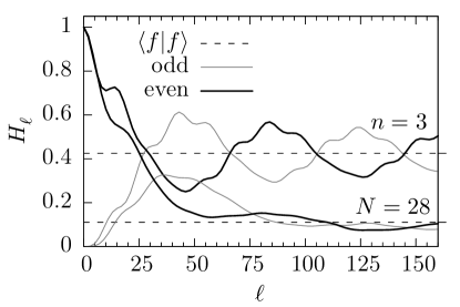
(a) 2-jet-like

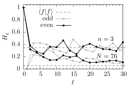
(b) 3-jet-like

Figure 1: The power spectra for two $e^{+}e^{-}\to q\bar{q}g$ events at $\sqrt{S}=\text{250}\,\text{GeV}$ which are (a) 2-jet-like and (b) 3-jet-like. Lines connect even and odd moments at integer $\ell$. Each figure shows $H_{\ell}$ for (upper) $n=3$ initiating partons and (lower) $N=\mathcal{O}(50)$ measurable particles (after showering and hadronization). A dotted line shows the value of $\left\langle f|f\right\rangle$ for each series, and the inset depicts the energy and orientation of the original partons.

The power spectra of the 3-jet-like event in Fig. 1b is very different from the 2-jet-like event. As expected, an event with three distinct jets has a significant 3-prong power, since $H_{3}\approx H_{2}\approx 1/3$. Jet structure has a stronger influence over $H_{\ell}$, since the measurable and 3-parton spectra diverge at a much lower $\ell$. However, the most critical feature is the flattening of $H_{\ell}$ in Fig. 1 to an asymptotic plateau at $\left\langle f|f\right\rangle$, which drives a divergence in the total power. This is a symptom of a serious flaw in $H_{\ell}$; the $\delta$-distributions in the series approximation of $\rho(\hat{r})$ in the $Y_{\ell}^{m}$ basis (Eq. 3) is incomplete and never converges. A $Y_{\ell}^{m}$ decomposition is only complete when the function is square-integrable (i.e., $\int_{\Omega}\text{d}\Omega\,\rho^{2}(\hat{r})<\infty$), and $\delta$-distributions are not. We will see next that this problem is related to the limited angular resolution of a finite sample, and develop a remedy.

II.2 Angular resolution of a finite sample

In order to understand the power spectrum’s asymptotic plateau, and certain detector artifacts which we expect to see in measured power spectra, we briefly examine a toy model. Imagine a collision process that scatters particle energy isotropically and homogeneously across the sphere. This model’s trivial event shape $\rho(\hat{r})=1/(4\pi)$ has a featureless power spectrum: $H_{\ell}=0$ for $\ell>0$. Yet when we simulate this process, the power spectra are not featureless — primarily because each event has a finite number of particles (and is therefore inhomogeneous), but further because detectors do not perfectly measure particle positions. Two irreducible detector effects create important angular artifacts: (i) the inactive beam hole, and (ii) the reduced angular precision of calorimeter towers. To study these effects, we construct a nearly truth-level pseudo-detector, through which we pass isotropic events built from $N$ generic particles. Each event is detected twice; first by making every particle charged (a track-only detection to study the beam hole effect), then by making all particles neutral (a tower-only detection to study the calorimeter effect). Each track or tower becomes a $\delta$-distribution in the Fox-Wolfram event shape (Eq. 5), whose $H_{\ell}$ is calculated via Eq. 7. The power spectra of four such events, with widely varying particle multiplicity $N$, are shown in Fig. 2 (which now connect adjacent $\ell$ with lines).

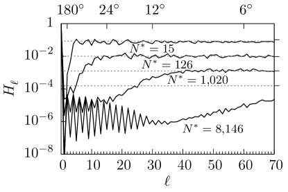
(a) tracks

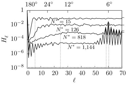
(b) towers

Figure 2: The power spectrum of isotropic samples of size $N=\{16,128,1024,8192\}$, seen with a pseudo-detector (using 1,144 towers of $\Omega_{\text{twr}}\approx(6^{\circ})^{2}$, $\eta_{\max}^{\text{trk}}=\eta_{\max}^{\text{twr}}\approx 3$, and $p_{T}^{\min}=0$). Each series is labeled by the number of objects $N^{*}$ actually detected, with (a) the entire sample detected as charged tracks and (b) the entire sample detected as neutral towers. A horizontal tick on the right edge depicts each sample’s $\left\langle f|f\right\rangle$.

Figure 2a’s track-only power spectrum confirms the isotropy of the samples; ${H_{\ell}\approx 0}$ for $\ell>0$ (note the log-scale). As particle multiplicity increases, the samples become increasingly homogeneous, further diminishing the residual non-zero power. But the falling power uncovers an oscillation at low $\ell$, a symptom of the handful of particles which escape detection through the beam holes. Since the angular scale of each moment in $H_{\ell}$ is $\xi=2\pi/\ell$ (Eq. 9), the correlations between two opposing holes emanate from their fundamental ${\ell=2}$ mode. This beam-hole artifact is fully evident only in the high-multiplicity samples because one must cover the sphere quite thoroughly before detecting two small holes. Fortunately, the $\mathcal{O}(10^{-5})$ power of the beam-hole artifact is quite small, so it is swamped by random sampling noise in low-multiplicity samples.

Another important feature in Fig. 2a is the power spectrum’s flat asymptotic plateau We can explain this plateau by splitting the power spectrum of the Fox-Wolfram event shape into constant self and $\ell$-dependent inter-particle correlations:

$$H_{\ell}=\underset{\text{self}}{\underbrace{\left\langle f|f\right\rangle}}+\underset{\text{inter-particle}}{\underbrace{\left\langle f\right|\left(P_{\ell}\big{(}\left|\hat{p}\right\rangle\cdot\left\langle\hat{p}\right|\big{)}-\text{{\small$1$}}1\right)\left|f\right\rangle}}\,.$$ (10)

As $\ell$ increases, inter-particle correlations are analyzed at increasingly smaller angular scales. Eventually, one reaches $\xi_{\min}$: the angular scale of the smallest inter-particle angles. At smaller scales (higher $\ell$), $H_{\ell}$ begins to probe the empty space between nearest neighbors, which is dominated by random sampling noise (i.e., the exact location of each $\delta$-distribution relative to all others); this causes the inter-particle correlations to interfere destructively. The remaining “self” term creates a featureless, asymptotic plateau at ${H_{\ell}\sim\left\langle f|f\right\rangle}$ (each sample’s $\left\langle f|f\right\rangle$ is shown with a horizontal tick on the graph’s right edge).

Since the asymptotic plateau is born in the transition from useful information to noise, the plateau effectively defines a power spectrum’s angular resolution. The high-multiplicity samples in Fig. 2a have lower plateaus which begin at higher $\ell$, so they are better able to discern the high-$\ell$ components of the beam-hole artifact. This relationship to multiplicity is made more explicit in Appendix A, where we show that $\left\langle f|f\right\rangle$ has an expected value of

$$\text{Ex}\left(\left\langle f|f\right\rangle\right)=\frac{1+a}{N}\,,$$ (11)

where $a\geq 0$, and depends on the probability distribution of the particles’ energy fraction. The dotted lines in Fig. 2a show this prediction for $a\approx 0.278$ (a value determined in Ref. Pedersen (2018) for our isotropic sampling); this prediction agrees quite well with each plateau’s actual height. Unfortunately, Eq. 11 does not divulge the angular resolution, it merely shows that it is somehow related to multiplicity.

To quantify a sample’s angular resolution, we examine Fig. 2b, whose tower-only power spectrum induces an artificial $\ell=60$ correlation (corresponding to the $6^{\circ}$ separation of nearest neighbor towers). While this occurs in every sample, its angular artifact is only visible in the high-multiplicity samples where particles have activated multiple towers. Ultimately, the poor angular resolution of the low-multiplicity samples is driven by their sparseness; in the $N^{*}=15$ sample of Fig. 2b, the closest particles are $18^{\circ}$ apart — too distant to uncover a $6^{\circ}$ correlation. This further demonstrates that $H_{\ell}$ cannot resolve correlations much beyond the smallest inter-particle angles. Furthermore, multiplicity is not the only factor; 15 particles in two intensely collimated, back-to-back jets will have a much finer angular resolution than 15 particles distributed isotropically, since the collimated particles in the former will be much closer together.

Given that the scale of the smallest inter-particle angles defines a sample’s angular resolution, we give $\xi_{\min}$ a rigorous definition by appealing to the $H_{\ell}$ inter-particle term in Eq. 10. First, the symmetric matrices of inter-particle angles ${\xi_{ij}\equiv\arccos(\hat{p}_{i}\cdot\hat{p}_{j})}$ and correlation weights $w_{ij}=f_{i}f_{j}$ are flattened into vectors $\left|\xi\right\rangle$ and $\left|w\right\rangle$ (keeping only $j>i$, since the lower-half of $\xi_{ij}$ is redundant, and its diagonal is null). We then sort $\left|\xi\right\rangle$ from smallest to largest, sequencing $\left|w\right\rangle$ to this new order. A legitimate inter-particle correlation must stand out from the asymptotic plateau of self-correlations, so we find the first $n$ angles whose collective weight is larger than $\left\langle f|f\right\rangle$ (i.e., $n$ is the first index where $\sum_{k=1}^{n}2\,w_{k}\geq\left\langle f|f\right\rangle$). The angular resolution $\xi_{\min}$ can then be computed from the weighted geometric mean of these $n$ smallest angles:

$$\xi_{\min}=\exp\left(\frac{\sum_{k=1}^{n}w_{k}\,\log\xi_{k}}{\sum_{k=1}^{n}w_{k}}\right)\,.$$ (12)

In Fig. 2b we calculate each sample’s $\xi_{\min}$, then use Eq. 9 to convert this angular resolution to $\ell_{\max}$: the maximum usable $H_{\ell}$ (shown with a dotted line).

Recall that we defined the angular resolution in terms of the smallest meaningful inter-particle correlation which, according to Eq. 10, should mark the beginning of the asymptotic plateau. If we look at the two low-multiplicity samples in Fig. 2b, their $\ell_{\max}$ occurs directly after the start of their respective plateaus — our definition of $\xi_{\min}$ is self-consistent. Note that in the $N^{*}=126$ sample, a small $\ell=60$ correlation is still visible beyond its $\ell_{\max}$. This occurs because two particles separated at $12^{\circ}$ can also enhance a $6^{\circ}$ correlation, which makes $\xi_{\min}$ a conservative estimate of the angular resolution. Nonetheless, $\xi_{\min}$ correctly identifies when $H_{\ell}$ has settled into its asymptotic plateau, and likely contains no further information (note that in the two high-resolution samples, the flat plateau is replaced by the angular artifact of the saturated calorimeter lattice, with repeating overtones as $\ell\to\infty$). We have established a link between event multiplicity $N$ and angular resolution, and used it to define a conservative estimate for the angular resolution. In the next Section, we modify the Fox-Wolfram assumptions and determine how to use the angular resolution to discard spurious, high-$\ell$ correlations.

III Shape functions as low-pass filters

In order to remove high-$\ell$ correlations that are dominated by sampling noise, we require a low-pass filter. Defining a filter is complicated because each event contains a distinct angular resolution. Simply cutting off $\ell>\ell_{\max}$ (a step function) would work, but that scheme gives equal weight to $\ell=2$ and $\ell=\ell_{\max}$, even though the coarse angular scale of $\ell=2$ makes it far less sensitive to small perturbations. Instead we want to use a shape function that emphasizes low $\ell$ moments and suppresses high $\ell$ moments. In addition, our function will have the advantage that experimental resolutions can be incorporated into the theoretical predictions.

While the discrete event shape $\rho(\hat{r})$ of Eq. 5 was the simplest, most compact way of summarizing an event’s energy distribution from a finite sample, its $\delta$-distributions imply that each particle’s angular position $\hat{p}_{i}$ is known with infinite angular resolution. In order to accommodate finite angular resolution, we build a low-pass filter into each particle’s angular position — distributing each particle in space using a continuous shape function $h_{i}(\hat{r})$:

$$\rho(\hat{r})=\sum_{i=1}^{N}f_{i}\,h_{i}(\hat{r})\,.$$ (13)

The shape function smears each particle about its observed location $\hat{p}_{i}$, preserving its coarse location, but reducing the angular resolution of $\rho(\hat{r})$.

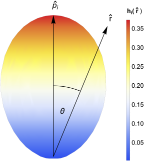
Figure 3: A plot of a particle shape function $h_{i}(\hat{r})$ that is pseudo-Gaussian in polar angle $\theta$ (relative to the particle’s observed direction of travel $\hat{p}_{i}$).

We are free to choose nearly any shape which is normalizable ($\int_{\Omega}\text{d}\Omega\,h(\hat{r})=1$) and acts as a low-pass filter. A natural choice is azimuthally symmetric about $\hat{p}_{i}$ and pseudo-normal in polar angle $\theta_{i}$ (where $\cos\theta_{i}\equiv\hat{r}\cdot\hat{p}_{i}$):

$$h_{i}(\hat{r})=\frac{1}{2\pi\lambda^{2}(1-e^{-2/\lambda^{2}})}\exp\left(-\frac{(1-\hat{r}\cdot\hat{p}_{i})}{\lambda^{2}}\right)\overset{\lambda\ll 1}{\approx}\frac{1}{2\pi\lambda^{2}}\exp\left(-\frac{\theta_{i}^{2}}{2\lambda^{2}}\right)\,,$$ (14)

This choice has the advantage that it reduces to a Gaussian in the small angle limit — a form that maps to the leading Sudakov form factor in angular-ordered showering. To relate this distribution’s width $\lambda$ to the sample’s angular resolution $\xi_{\min}$, we solve for the $\lambda$ which encloses a fraction $u\in[0,1]$ of each particle within a circular cap of angular radius $R$:

$$\lambda=\sin\left(\frac{R}{2}\right)\sqrt{\frac{-2}{\log(1-u(1-e^{-2/\lambda^{2}}))}}\,.$$ (15)

Setting $R=\xi_{\min}$, this transcendental equation can be solved recursively (starting with $\lambda=0$).

However, by giving particles an extensive shape we can no longer use the simple linear algebra of Eq. 7 — we must return to original definition:

$$H_{\ell}\equiv\frac{4\pi}{2\ell+1}\sum_{m=-\ell}^{\ell}\left|\rho_{\ell}^{m}\right|^{2}\,.$$ (16)

The $\rho_{\ell}^{m}$ integral for a continuous, multi-pronged event shape is not trivial. First we use the definition of $\rho(\hat{r})$ in Eq. 13 to separate the $\rho_{\ell}^{m}$ integral into each particle’s shape function

$$\rho_{\ell}^{m} =f_{1}\,{h_{(1)}}_{\ell}^{m}+f_{2}\,{h_{(2)}}_{\ell}^{m}+{\dots}+f_{N}\,{h_{(N)}}_{\ell}^{m}\,.$$ (17)

This permits the square modulus $\left|\rho_{\ell}^{m}\right|^{2}$ to be expanded into a series of terms like ${h_{(i)}}_{\ell}^{m}{h_{(j)}}_{\ell}^{m*}$. Using the $Y_{\ell}^{m}$ addition theorem, we can prove that each $H_{\ell}$ sub-term is rotationally invariant (like $H_{\ell}$ as a whole), since $\hat{r}$ and $\hat{r}^{\prime}$ fully factorize, save for the rotationally invariant $\hat{r}\cdot\hat{r}^{\prime}$;

$$\sum_{m=-\ell}^{\ell}{h_{(i)}}_{\ell}^{m}{h_{(j)}}_{\ell}^{m*} =\sum_{m=-\ell}^{\ell}\int_{\Omega}\text{d}\Omega\,{Y_{\ell}^{m}}^{*}(\hat{r})h_{(i)}(\hat{r})\int_{\Omega^{\prime}}\text{d}\Omega^{\prime}\,Y_{\ell}^{m}(\hat{r}^{\prime})h_{(j)}(\hat{r}^{\prime})$$ (18)

$$=\int_{\Omega}\text{d}\Omega\int_{\Omega^{\prime}}\text{d}\Omega^{\prime}\,h_{(i)}(\hat{r})h_{(j)}(\hat{r}^{\prime})P_{\ell}(\hat{r}\cdot\hat{r}^{\prime})\,.$$ (19)

We can therefore calculate each sub-term in whatever orientation is the simplest.

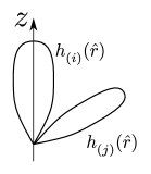
Figure 4: A pair of shape functions which have been rotated such that $h_{(i)}(\hat{r})$ is parallel to the $z$-axis (“up”), maintaining the interior angle with $h_{(j)}(\hat{r})$ (“out”).

A natural choice of orientation is depicted in Fig. 4: $h_{(i)}(\hat{r})$ is oriented “up” in the $Y_{\ell}^{m}$ system (parallel to the longitudinal $z$ axis), which tilts $h_{(j)}(\hat{r})$ “out.” Alternatively, the $j$ shape can be oriented “up,” with $i$ sticking “out.” Rotational invariance makes these choices equivalent, which we can express using an arrow to denote orientation ($\uparrow$ being “up” and $\nearrow$ being “out”)

$$\sum_{m=-\ell}^{\ell}{h_{(i)}^{\;\uparrow}}_{\ell}^{m}\,{h_{(j)}^{\nearrow}}_{\ell}^{m}=\sum_{m=-\ell}^{\ell}{h_{(i)}^{\nearrow}}_{\ell}^{m}\,{h_{(j)}^{\;\uparrow}}_{\ell}^{m}\,.$$ (20)

Now let us constrain $\rho(\hat{r})$ to only use shape functions which are azimuthally symmetric about their central axis. This forces all “up” coefficients to zero except $m=0$, which collapses the inner products on both sides of the equation to

$${h_{(i)}^{\;\uparrow}}_{\ell}^{0}\,{h_{(j)}^{\nearrow}}_{\ell}^{0}={h_{(i)}^{\nearrow}}_{\ell}^{0}\,{h_{(j)}^{\;\uparrow}}_{\ell}^{0}\,.$$ (21)

Recall that these coefficients are independent scalars from separate integrals (see Eq. 18); not only will Eq. 21 hold for any azimuthally symmetric $j$ shape, choosing a particular $j$ shape cannot impose any constraints on the $i$ shape.

We now choose $h_{(j)}(\hat{r})=\frac{\delta^{2}(\hat{r}-\hat{p}_{j})}{\sin\theta_{j}}$, a shape whose coefficients are trivial: ${h_{(j)}^{\;\uparrow}}_{\ell}^{0}=1$ and ${h_{(j)}^{\nearrow}}_{\ell}^{0}=P_{\ell}(\hat{p}_{i}\cdot\hat{p}_{j})$. Plugging these into Eq. 21, it simplifies to

$${h_{(i)}^{\nearrow}}_{\ell}^{0}\,={h_{(i)}^{\;\uparrow}}_{\ell}^{0}\,P_{\ell}(\hat{p}_{i}\cdot\hat{p}_{j})\,.$$ (22)

Regardless of the shape of $h_{(i)}(\hat{r})$, its “out” coefficient can be calculated from its “up” coefficient. Using an overline to signify a scaled, $m=0$ “up” coefficient

$${{}\bar{h}_{(i)}}_{\ell}\equiv\sqrt{\frac{4\pi}{2\ell+1}}{h_{(i)}^{\;\uparrow}}_{\ell}^{0}=\int_{\Omega}\text{d}\Omega\,P_{\ell}(\hat{r}\cdot\hat{z})\,h_{(i)}^{\;\uparrow}(\hat{r})\,,$$ (23)

each sub-term in the $H_{\ell}$ expansion simplifies to

$$\frac{4\pi}{2\ell+1}\sum_{m=-\ell}^{\ell}{h_{(i)}}_{\ell}^{m}{h_{(j)}}_{\ell}^{m*}={{}\bar{h}_{(i)}}_{\ell}\,{{}\bar{h}_{(j)}}_{\ell}\,P_{\ell}(\hat{p}_{i}\cdot\hat{p}_{j})\,.$$ (24)

Therefore, given an event shape $\rho(\hat{r})$ composed solely from particles with azimuthally symmetric shape functions, its power spectrum is

$$H_{\ell}=(f_{i}\,{{}\bar{h}_{(i)}}_{\ell})\,P_{\ell}(\hat{p}_{i}\cdot\hat{p}_{j})\,(f_{j}\,{{}\bar{h}_{(j)}}_{\ell})\,\,.$$ (25)

If every particle uses the same shape function, then this simplifies to an $\ell$-dependent prefactor that scales the raw, discrete power spectrum of Eq. 7,

$$H_{\ell}={}\bar{h}_{\ell}^{2}\times\left\langle f\right|P_{\ell}\big{(}\left|\hat{p}\right\rangle\cdot\left\langle\hat{p}\right|\big{)}\left|f\right\rangle\,.$$ (26)

This last scenario is the simplest use-case for shape functions — calculate the sample’s angular resolution $\xi_{\min}$, then create one pseudo-normal shape that smears each particle by an appropriate $\lambda$. According to Eq. 26, plotting ${}\bar{h}_{\ell}^{2}$ for this shape will reveal its band limit, and we show several values of $\lambda$ in Fig. 5 (see Appendix B for the detailed calculation of ${}\bar{h}_{\ell}$). This plot demonstrates that the pseudo-normal shape acts as an ideal low-pass filter; it preserves information at low $\ell$, and gradually discards information as $\ell$ increases. As seen in Fig. 5b, ${}\bar{h}_{\ell}$ eventually enters an approximately exponential decay which removes $H_{\ell}$’s asymptotic plateau. This has a meaningful interpretation — the discrete event shape created a plateau in $H_{\ell}$ because $\delta$-distributions contain every frequency (${}\bar{h}_{\ell}=1$). A coarse-graining provided by extensive shapes imposes a band limit though the asymptotic decay of their ${}\bar{h}_{\ell}$.

(a)

(b)

Figure 5: The squared “up” coefficient ${}\bar{h}^{2}_{\ell}$ for the pseudo-normal shape function, with several smearing angles $\lambda$ on a (a) linear and (b) log-linear scale.

III.1 Shape functions for measurement uncertainty

Thus far, we have used shape functions to discard small-angle sampling noise in an under-sampled distribution, so that we can focus on an its large-angle structure. However, we can also use shape functions more traditionally: to encapsulate measurement uncertainty. For example, if one particular charged track is poorly measured, then its angular uncertainty may exceed the sample’s $\xi_{\min}$, and its individual shape function should be driven by its measurement uncertainty. A more important case is calorimeter towers, whose intrinsic angular uncertainty dwarfs that of tracks, and usually even $\xi_{\min}$.

A calorimeter is built from multiple layers of cells with varying segmentation and sensitivity, and non-overlapping centers. This provides detailed information about the depth and breadth of the induced particle shower. “Towers” are not bins of energy with clean edges. Sophisticated modeling and reconstruction algorithms should be able to build a probability distribution for the angular position of a tower’s initiating particle, but such modeling is beyond the scope of this paper. Instead we consider a pseudo-detector built of towers that use a uniform circular cap of angular radius $R$, which provides azimuthal symmetry and a decent approximation for the tower (even though the edges are wrong, it creates a low-pass filter at the correct scale). We calculate ${}\bar{h}_{\ell}$ coefficients for a uniform circular cap in Appendix B.

Consider a track landing near a tower’s centroid; while the track-centroid angle ${\xi_{ij}\equiv\arccos(\hat{p}_{i}\cdot\hat{p}_{j})}$ is small, we cannot pinpoint where the energy was deposited. We should therefore use the angle between the two objects, which averages over their constituent shape functions:

$$\xi_{ij}^{*}=\int\text{d}\Omega\int\text{d}\Omega^{\prime}\,h_{(i)}(\hat{r})\,h_{(j)}(\hat{r}^{\prime})\arccos(\hat{r}\cdot\hat{r}^{\prime})\,.$$ (27)

Thus, $\xi_{ij}^{*}$ is used to calculate $\xi_{\min}$ (leading to a larger value than estimated by Eq. 12). While calculating $\xi_{\min}$, tracks should use a shape function based upon their individual measurement uncertainty. Once the angular resolution is known, $\xi_{\min}$ sets the minimum smearing for all objects, and tracks should be smeared with the pseudo-normal shape. Note that $H_{\ell}$ already accounts for extensive objects; the extensive angle (Eq. 27) is only needed for $\xi_{\min}$.

Figure 6: The dimensionless angular separation between objects, showing the relationship between the extensive angle $r^{*}$ and the raw, inter-centroid angle $r$. The two are equivalent between well-measured tracks. Approximating towers as uniform circular caps, the result of numerical integration ($\circ$) are fit by the pseudo-hyperbola (Eq. 29) for the (t)rack-(T)ower angle ($R_{i}=0$, $R_{j}=1^{\circ}$) and the (T)ower-(T)ower angle ($R_{i}=R_{j}=1^{\circ}$).

In this paper we use a pseudo-detector which assumes exceptional tracking, such that the difference between $\xi_{ij}^{*}$ and $\xi_{ij}$ is dominated by towers. It is therefore safe to treat tracks as $\delta$-distributions, so that (t)rack-(t)rack angles can use $\xi^{*}_{\text{tt}}=\xi$. To calculate the (T)ower-(T)ower extensive angle $\xi^{*}_{\text{TT}}$, we switch to a relative angular distance $r$: the inter-tower angle scaled by the angular radius of the two-tower system $R_{ij}=\sqrt{R_{i}^{2}+R_{j}^{2}}$;

$$r_{ij} \equiv\frac{\xi_{ij}}{R_{ij}}\,, r^{*}_{ij} \equiv\frac{\xi^{*}_{ij}}{R_{ij}}\,.$$ (28)

By sending $R_{i}\to 0$, this $r$ also works for the (t)rack-(T)ower angle $\xi^{*}_{\text{tT}}$.

Using the scale-free angle $r$ uncovers a nearly universal mapping $\xi\mapsto\xi^{*}$, shown in Fig. 6. As an object approaches a tower, the extensive angle $\xi^{*}$ approaches a minimum value. Conversely, as the tower gets farther away, it appears increasingly discrete and $\xi^{*}\sim\xi$. The shape of this curve is well-approximated by the pseudo-hyperbolic function

$$r^{*}(r)=(a^{b}+r^{b})^{\frac{1}{b}}\,.$$ (29)

The best-fit parameters accompanying Fig. 6 demonstrate that track-tower angles $r^{*}_{\text{tT}}(r)$ and tower-tower angles $r^{*}_{\text{TT}}(r)$ are barely distinguishable as $r\to 0$. Towers with non-matching radii ($R_{i}\neq R_{j}$) exist on an intermediate curve. Importantly, these curves are effectively scale-free until the two-tower radius scale $R_{ij}$ grows very large (about $30^{\circ}$), at which point the exponent $b$ becomes larger, causing a faster decay to the asymptote. Both fits are systematically biased in a few places (e.g., a slight overestimation near $r=1$), but recall that the angular resolution (Eq. 12) uses the geometric mean to average over scales. Thus, it is far better to use $r^{*}_{\text{tT}}(r)$ to get a conservative estimate for $\xi_{ij}^{*}$, rather than using the raw centroid angle $\xi_{ij}$, which would claim that a track striking a tower’s center is a well-measured, small-angle correlation.

III.2 Infrared and collinear safety

In this section, we have taken the QCD radiation spectrum of Fox and Wolfram and expanded it with a comprehensive framework of shape functions to account for sampling granularity and measurement uncertainty. Putting these pieces together for the first time, we immediately see that shape functions are essential for keeping $H_{\ell}$ infrared and collinear safe. This is the final piece we need to use the QCD radiation spectrum.

Let us return to the two events of Fig. 1, which were analyzed via a truth-level detection of their measurable final-state particles. We now filter those particles through our pseudo-detector (using $\Omega_{\text{twr}}=(6^{\circ})^{2}$, and cuts $\eta_{\max}^{\text{trk}}=\eta_{\max}^{\text{twr}}=3$, and $p_{T}^{\min}=\text{300}\,\text{MeV}$), calculate the angular resolution $\xi_{\min}$ using extensive inter-particle angles $\xi^{*}_{ij}$, then smear the tracks via a pseudo-normal shape function to calculate $H_{\ell}$ (solving $\lambda$ for $u=90\%$ of the track shape within in a cap of radius $R=\xi_{\min}$). This scheme produces a smooth event shape $\rho(\hat{r})$ with a sample’s “natural resolution.” Yet examining its power spectrum by eye does not provide much insight — it looks like the moments in Fig. 1 multiplied by a low-pass filter similar to Fig. 5. Luckily, there is a much more physical way to view the power spectrum.

In their seminal papers Fox and Wolfram (1978, 1979), Fox and Wolfram introduced an “autocorrelation” function which we relabel the “angular correlation function;” it uses $H_{\ell}$ as the coefficients in a Legendre series for inter-particle angle $\xi$:

$$F(\cos\xi)=\sum_{\ell=0}^{\infty}(2\ell+1)H_{\ell}\,P_{\ell}(\cos\xi)\,.$$ (30)

The area under the angular correlation function is always two (since $\int_{-1}^{1}\text{d}z\,P_{\ell}(z)=2\,\delta_{\ell}^{0}$ and $H_{0}=1$). A peak at $\cos\xi$ indicates that energy within the sample is correlated at that angle, with the area under the peak equal to the collective weight $w=4\sum f_{i}f_{j}$ of all pairs separated by $\xi$ (relative to each other, not to any particular axis). For example, events containing prongs of collinear energy should have a large $F$ at $\cos\xi=1$.

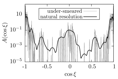
(a) 2-jet-like

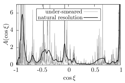
(b) 3-jet-like

Figure 7: The angular correlation function for two $e^{+}e^{-}\to q\bar{q}g$ events at $\sqrt{S}=\text{250}\,\text{GeV}$ which are (a) 2-jet-like and (b) 3-jet-like.

Clearly, if $H_{\ell}$ flattens to an asymptotic plateau, $F$ will never converge for finite $l$, so it is not actually possible to plot $F$ from the Fox-Wolfram event shape. However, we can create a nearly discrete event shape by smearing every detected track or tower with a pseudo-Gaussian ten times thinner than the one prescribed by the sample’s angular resolution $\xi_{\min}$. In Figure 7, we compare this “under-smeared” $\rho(\hat{r})$ to the natural resolution shape. The difference is quite striking. For both events, the under-smeared $F$ contains extremely narrow correlations from individual particle pairs. Conversely, the appropriate amount of smearing gathers these ultra-fine details into a smooth peak. This permits us to verify the event’s overall shape: the 2-jet-like event (Fig. 7a, shown on a log-scale) is extremely back-to-back, since the largest correlation other than $\cos\xi=\pm 1$ is incredibly small (i.e., $F(\cos 90^{\circ})\approx 0.1$). This is much different than the 3-jet-like event (Fig. 7b), which has three large peaks at $\cos\xi<0$, corresponding to the three inter-jet angles (c.f. the inset of Fig. 1b).

It is clear, given the weight ${w_{ij}=f_{i}f_{j}}$ of each correlation, that $H_{\ell}$ (and thus $F$) is intrinsically insensitive to infrared radiation (which has $f\ll 1$ by definition). Figure 7 now shows that shape functions make $H_{\ell}$ insensitive to collinear radiation (the fine structure visible in the under-smeared $F$). This fine structure is only probed by high-$\ell$ moments (Eq. 9), a relationship we can make explicit by examining a particle splitting to two nearly parallel particles ($a\to b\,c$). First we examine $a$’s total contribution to the power spectrum before the splitting (where $z_{aj}\equiv\hat{p}_{a}\cdot\hat{p}_{j}$)

$$H_{\ell,\,a}=f_{a}\sum_{j}f_{j}\,P_{\ell}(z_{aj})\,.$$ (31)

When particle $a$ splits, $\hat{p}_{b/c}=\hat{p}_{a}+\vec{\delta}_{b/c}$ (for tiny $\vec{\delta}_{b/c}$), this contribution becomes

$$H_{\ell,\,a} =f_{b}\sum_{j}f_{j}P_{\ell}(z_{aj}+\delta z_{bj})+f_{c}\sum_{j}f_{j}P_{\ell}(z_{aj}+\delta z_{cj})\,.$$

Because ${f_{a}=f_{b}+f_{c}}$, the total contribution $H_{\ell,\,a}$ is perturbed only in the $P_{\ell}$ terms. And only when $\ell$ becomes large — so that $P_{\ell}(z)$ is highly oscillatory at the scale of $\delta z$ — can a small $\delta z$ give rise to significant changes in $H_{\ell}$. Hence, a low-pass filter tailored to an event’s information content is essential for keeping the power spectrum infrared and collinear safe. With this we now have a complete framework in which to encode the full energy and angular correlated information of a QCD event.

IV Conclusions

In this paper we address some deficiencies of the energy-weighted QCD angular power spectrum and its artifacts due to finite sampling. We extend the power spectrum introduced by Fox and Wolfram Fox and Wolfram (1978, 1979) by replacing an energy density distribution constructed out of measured point-like particles with a shape function that acts as a band pass filter to suppress these artifacts. The shape function naturally accommodates the measurement resolutions of tracks and calorimeter cells, and other experimental complications, such as false peaks arising from holes in the detector. While our shape function maps directly to leading QCD radiation at small angles, other functions that preserve the smallest measurable angle constraint could be used to more adequately map out detector-dependent shapes unique to a particular design.

By construction, the moments $H_{\ell}$ of the power spectrum are infrared safe. Our use of shape functions to smear an event to its sampled resolution guarantees collinear safety by discarding correlations at angular scales smaller than the information content of the event. Hence, we have established a framework in which information encoded in the power spectrum can be used to extract well-defined observables using the fully-correlated data from an entire QCD event.

The next step is to build studies to explore QCD phenomena at all scales. An initial foray may be found in Refs. Sullivan and Pedersen (2019); Pedersen et al. , where jet-like physics in $e^{+}e^{-}$ events is extracted with higher precision than that provided by current sequential jet algorithms in the presence of pileup. We should also improve theoretical predictions by calculating next-to-leading order corrections to the QCD power spectrum itself. From there we can begin to map the effects of jet substructure — noting that we will capture the effects of radiation emitted at angles larger than normally captured by sequential jet definitions.

This paper focuses on $e^{+}e^{-}$ events and calculations in the center of momentum frame which can be derived analytically. While it is straightforward to compute the power spectrum for hadronic collisions, it can only be performed numerically. The next step is to provide the boosted calculations necessary to compare numerical simulations of the power spectrum to QCD jet data provided by the ATLAS and CMS Collaborations at the CERN Large Hadron Collider. Finally, if a power spectrum can be calculated using the fundamental QCD degrees of freedom found in heavy-ion collisions, this framework can be used to understand short- and long-range correlations in heavy ion data on an event-by-event basis.

Appendix A Connecting $\boldsymbol{\left\langle f|f\right\rangle}$ to particle multiplicity $\boldsymbol{N}$

In Section II we explore the consequences of the connection between $\left\langle f|f\right\rangle$ and particle multiplicity. In this appendix we present the derivation of the relationship (taken from Ref. Pedersen (2018)).

A.1 Why $\boldsymbol{\left\langle f|f\right\rangle\propto N^{-1}}$

To study the expected value $\text{Ex}\left(\left\langle f|f\right\rangle\right)$, we assume that there is a generic physics process where particle energy follows some smooth probability distribution $h(E)$, but where particle multiplicity $N$ is variable. Converting this $h(E)$ distribution to energy fraction $h(f)$, we find the undesirable property that the mode scales with $N$ (since the mean $\text{Ex}\left(f\right)=N^{-1}$ by construction). It is therefore useful to define the scale-free energy fraction

$$\tilde{f}\equiv\frac{f}{\text{Ex}\left(f\right)}=Nf\,.$$ (32)

We then require that $h(\tilde{f})$ has a finite variance

$$\text{Var}(\tilde{f})=\text{Ex}(\tilde{f}^{2})-\text{Ex}(\tilde{f})^{2}=\text{Ex}(\tilde{f}^{2})-1\,.$$ (33)

We now construct an energy fraction vector $\left|f\right\rangle$ for a random instance of this physics process; we draw $N$ energy fractions $\tilde{f}$ from $h(\tilde{f})$, then normalize to their sum:

$$\left|f\right\rangle=\frac{\{\tilde{f}_{1},\tilde{f}_{2},\dots,\tilde{f}_{N}\}}{\tilde{f}_{1}+\tilde{f}_{2}+\dots+\tilde{f}_{N}}\,.$$ (34)

The expectation value of $\left\langle f|f\right\rangle$ is therefore

$$\text{Ex}\left(\left\langle f|f\right\rangle\right)=\int\text{d}\tilde{f}_{1}\,\text{d}\tilde{f}_{2}\dots\text{d}\tilde{f}_{N}\frac{\tilde{f}_{1}^{2}+\tilde{f}_{2}^{2}+\dots+\tilde{f}_{N}^{2}}{(\tilde{f}_{1}+\tilde{f}_{2}+\dots+\tilde{f}_{N})^{2}}\,h(\tilde{f}_{1})\,h(\tilde{f}_{2})\dots h(\tilde{f}_{N})\,.$$ (35)

Provided that each $\tilde{f}_{i}$ is independent (i.e., all correlations are built into the shape of $h(\tilde{f})$), we can treat each $\tilde{f}_{i}$ separately and use the linearity of expectation to obtain

$$\text{Ex}\left(\left\langle f|f\right\rangle\right)=\frac{N\,\text{Ex}(\tilde{f}^{2})}{(N\,\text{Ex}(\tilde{f}))^{2}}=\frac{1}{N}\,\text{Ex}(\tilde{f}^{2})=\frac{1}{N}(1+\text{Var}(\tilde{f}))\,.$$ (36)

Thus, we expect the height of the power spectrum’s asymptotic plateau ${H_{\ell}\sim\left\langle f|f\right\rangle}$ to be inversely proportional to particle multiplicity, but somewhat larger than $1/N$ since ${\text{Var}(\tilde{f})\geq 0}$.

A.2 The smallest possible $\boldsymbol{\left\langle f|f\right\rangle_{\min}=N^{-1}}$

As a check of Eq. 36, we calculate the smallest possible value of $\left\langle f|f\right\rangle$ without assuming some well-behaved physics process with a limiting distribution $h(\tilde{f})$. We define a normalized energy fraction vector for some arbitrary set of particles:

$$\left|f\right\rangle=\left\{f_{1},\,\dots,\,f_{N-1},\,f_{N}\right\},\qquad\text{where}\quad f_{N}\equiv\Big{(}1-\sum_{i=1}^{N-1}f_{i}\Big{)}\geq 0\,.$$ (37)

Evaluating the gradient $\vec{\nabla}\left\langle f|f\right\rangle$, each energy fraction $f_{i}$ minimizes $\left\langle f|f\right\rangle$ when

$$\partial_{i}\left\langle f|f\right\rangle=\partial_{i}(f_{i}^{2}+f_{N}^{2})=2(f_{i}-f_{N})=0\,.$$ (38)

Thus, $\left\langle f|f\right\rangle$ is minimized when $f_{i}=f_{N}$, and if every energy fraction is equal to the final energy fraction, then all $f_{i}$ must be the same: $f_{i}=N^{-1}$. Therefore,

$$\left\langle f|f\right\rangle_{\min}=N(N^{-2})=\frac{1}{N}\,.$$ (39)

This result corresponds exactly to $\text{Var}(\tilde{f})=0$ for Equation 36.

Appendix B Calculating a shape function’s “up” coefficient $\boldsymbol{{}\bar{h}_{\ell}}$

The power spectrum $H_{\ell}$ for an event shape $\rho(\hat{r})$ built from azimuthally symmetric shape functions can be calculated using Eq. 25 — provided one knows the “up” coefficients ${}\bar{h}_{\ell}$ (Eq. 23). In this appendix we follow Ref. Pedersen (2018) to calculate ${}\bar{h}_{\ell}$ for the shape functions used in this paper. For each calculation, rotating the shape’s centroid “up” ($\hat{p}_{i}\mapsto\hat{z}$) permits the useful change of variable ${z\equiv\cos(\theta)=\hat{r}\cdot\hat{z}}$. Normalization constants will appear as $C$. Note that the ${}\bar{h}_{0}$ integral is simply the normalization condition, so ${}\bar{h}_{0}=1$ for every shape function.

B.1 The pseudo-normal shape function

The “up” coefficient (Eq. 23) for the pseudo-normal shape function (Eq. 14) is

$${}\bar{h}_{\ell}=\int_{0}^{2\pi}\text{d}\phi\int_{-1}^{1}\text{d}z\,P_{\ell}(z)\,C\,e^{-(1-z)/\lambda^{2}}=2\pi\,C\int_{-1}^{1}\text{d}z\,P_{\ell}(z)\,e^{-(1-z)/\lambda^{2}}\,.$$ (40)

To compute this integral, we can use a Legendre identity

$$(2\ell+1)P_{\ell}(z)=\frac{\text{d}}{\text{d}z}\left[P_{\ell+1}(z)-P_{\ell-1}(z)\right]\,.$$ (41)

This allows us to define an integral $A_{\ell}\equiv{}\bar{h}_{\ell}/(2\pi\,C)$, and set it up for integration by parts:

$$A_{\ell}=\int_{-1}^{1}\text{d}z\,e^{-(1-z)/\lambda^{2}}P_{\ell}(z)=\int_{-1}^{1}\text{d}z\,e^{-(1-z)/\lambda^{2}}\frac{1}{2\ell+1}\frac{\text{d}}{\text{d}z}\left[P_{\ell+1}(z)-P_{\ell-1}(z)\right]\,.$$ (42)

The boundary term vanishes because $[P_{\ell+1}(\pm 1)-P_{\ell-1}(\pm 1)]=0$. The surviving term is

$$A_{\ell}=\frac{1}{2\ell+1}\int_{-1}^{1}\text{d}z\,\frac{e^{-(1-z)/\lambda^{2}}}{\lambda^{2}}(P_{\ell-1}(z)-P_{\ell+1}(z))=\frac{1}{\lambda^{2}(2\ell+1)}(A_{\ell-1}-A_{\ell+1})\,.$$ (43)

Since ${}\bar{h}_{\ell}\propto A_{\ell}$, this result can be rearranged into a recurrence relation for ${}\bar{h}_{\ell}$:

$${}\bar{h}_{\ell+1}=-(2\ell+1)\lambda^{2}\,{}\bar{h}_{\ell}+{}\bar{h}_{\ell-1}\,.$$ (44)

We initialize this recursion with ${}\bar{h}_{0}=1$ (i.e., $h(\hat{r})$ is normalized) and

$${}\bar{h}_{1}=\frac{1}{\tanh(\lambda^{-2})}-\lambda^{2}\,.$$ (45)

For a demonstration of how to correct the recursion’s numerical instability as ${}\bar{h}_{\ell}\to 0$ see Ref. Pedersen (2018) .

B.2 A circular cap

To approximate calorimeter towers as uniform circular caps of angular radius $R$ and solid angle $\Omega_{\text{twr}}=2\pi\,(1-\cos R)$, we integrate upwards from $z=\cos R=1-a$ (where $a\equiv\frac{\Omega_{\text{twr}}}{2\pi}$):

$${}\bar{h}_{\ell}=\frac{1}{\Omega_{\text{twr}}}\int_{0}^{2\pi}\text{d}\phi\int_{1-a}^{1}\text{d}z\,P_{\ell}(z)=\frac{1}{a\,(2\ell+1)}[P_{\ell-1}(1-a)-P_{\ell+1}(1-a)]\,.$$ (46)

This uses Eq. 41 to integrate $P_{\ell}(z)$, and relies on the identity $[P_{\ell+1}(\pm 1)-P_{\ell-1}(\pm 1)]=0$.

References

- Ellis et al. (1981) R. K. Ellis, D. A. Ross, and A. E. Terrano, Nucl. Phys. B178, 421 (1981).
- Ellis and Soper (1993) S. D. Ellis and D. E. Soper, Phys. Rev. D48, 3160 (1993), eprint hep-ph/9305266.
- Cacciari et al. (2008) M. Cacciari, G. P. Salam, and G. Soyez, JHEP 04, 063 (2008), eprint 0802.1189.
- Larkoski et al. (2017) A. J. Larkoski, I. Moult, and B. Nachman (2017), eprint 1709.04464.
- Asquith et al. (2018) L. Asquith et al. (2018), eprint 1803.06991.
- Khachatryan et al. (2010) V. Khachatryan et al. (CMS), JHEP 09, 091 (2010), eprint 1009.4122.
- collaboration (2015) T. A. collaboration (2015).
- Calkins et al. (2013) R. Calkins, S. Chekanov, J. Conway, J. Dolen, R. Erbacher, J. Pilot, R. Poschl, S. Rappoccio, Z. Sullivan, and B. Tweedie, in Proceedings, 2013 Community Summer Study on the Future of U.S. Particle Physics: Snowmass on the Mississippi (CSS2013): Minneapolis, MN, USA, July 29-August 6, 2013 (2013), eprint 1307.6908, URL https://inspirehep.net/record/1244676/files/arXiv:1307.6908.pdf.
- Fox and Wolfram (1978) G. C. Fox and S. Wolfram, Phys. Rev. Lett. 41, 1581 (1978).
- Fox and Wolfram (1979) G. C. Fox and S. Wolfram, Nucl. Phys. B 149, 413 (1979), [Erratum: Nucl.Phys.B 157, 543 (1979)].
- Ellis et al. (1980) R. K. Ellis, D. A. Ross, and A. E. Terrano, Phys. Rev. Lett. 45, 1226 (1980).
- Vermaseren et al. (1981) J. A. M. Vermaseren, K. J. F. Gaemers, and S. J. Oldham, Nucl. Phys. B187, 301 (1981).
- Ali and Kramer (2011) A. Ali and G. Kramer, Eur. Phys. J. H36, 245 (2011), eprint 1012.2288.
- Basham et al. (1978) C. L. Basham, L. S. Brown, S. D. Ellis, and S. T. Love, Phys. Rev. Lett. 41, 1585 (1978).
- Fox and Wolfram (1980) G. C. Fox and S. Wolfram, Z. Phys. C4, 237 (1980).
- Ali and Barreiro (1982) A. Ali and F. Barreiro, Phys. Lett. 118B, 155 (1982).
- White and Srednicki (1995) M. White and M. Srednicki, Astrophys. J. 443, 6 (1995), eprint astro-ph/9402037.
- Alwall et al. (2014) J. Alwall, R. Frederix, S. Frixione, V. Hirschi, F. Maltoni, O. Mattelaer, H. S. Shao, T. Stelzer, P. Torrielli, and M. Zaro, JHEP 07, 079 (2014), eprint 1405.0301.
- Sjostrand et al. (2006) T. Sjostrand, S. Mrenna, and P. Z. Skands, JHEP 05, 026 (2006), eprint hep-ph/0603175.
- Sjostrand et al. (2008) T. Sjostrand, S. Mrenna, and P. Z. Skands, Comput. Phys. Commun. 178, 852 (2008), eprint 0710.3820.
- Pedersen (2018) K. Pedersen, Ph.D. thesis, Illinois Institute of Technology (2018).
- Sullivan and Pedersen (2019) Z. Sullivan and K. Pedersen, EPJ Web Conf. 206, 05005 (2019).
- (23) K. Pedersen, M. Mangedarage, and Z. Sullivan, in preparation.