Access Single Mode Approximation via Quantum Monte Carlo

Abstract

We extend the Single Mode Approximation (SMA) into quantum Monte Carlo (QMC) versions to obtain the dynamical dispersion of quantum many-body systems. Based on Stochastic Series Expansion (SSE) and its projector algorithms, we put forward the ways to realize the calculation of SMA within the SSE frame. The SMA + QMC method can quickly extract the dispersion of the dynamical spectrum without external calculations and high technique barriers. Meanwhile, numerical analytic continuation methods require the fine data of imaginary time correlations and complex programming. Therefore, our method can approach the excitation spectrum of large systems, e.g., we take the two-dimensional Heisenberg model on a $512\times 512$ square lattice. We demonstrate the effectiveness and efficiency of our method with high precision via additional examples.

I introduction

Strongly correlated systems emerge with many novel phenomena and thus attract much attention. Usually, exotic quantum states with peculiar behaviors do not thoroughly exhibit themselves in small systems due to finite-size effects. The exponentially increasing degree of freedom of the Hilbert space hinders further understanding of quantum many-body systems. This stimulates people to derive new approaches to more extensive system sizes. Quantum Monte Carlo (QMC) is a powerful numerical tool for dealing with complex systems, especially with a high degree of freedom [1].

Generally, there are two main branches of QMC methods. The first branch uses stochastic processes to simulate the finite temperature partition function of quantum many-body systems. This branch includes algorithms like Stochastic Series Expansion (SSE) [2, 3, 4, 5, 6, 7, 8] and path integral [9, 10, 11, 12]. The other one performs the ground state wave function at zero temperature, such as diffusion Monte Carlo [13, 14, 15, 16, 17] and Green’s function Monte Carlo [18, 19, 20, 21].

Although knowledge of the ground state is always what people seek in the first place, excited states and energy spectrum, which carry information on the energy gap and dynamical exponent $z$, also play a crucial role in our understanding of the system. Obtaining the excitation information of many-body systems is one of the most challenging tasks in QMC simulations. Some numerical analytical continuation methods [22, 23, 24, 25, 26, 27] like max entropy method and Stochastic Analytic Continuation (SAC) have been developed during the past decades, aiming at solving this problem [28, 29, 30, 31, 32, 33, 34, 35, 36]. However, massive computing resources are required to get excitation spectrum. Moreover, these algorithms need to fit each spectrum case by case, with modifications that may lead to ambiguous results, not to mention the fitting process itself could be time-consuming. Unfortunately, the computation complexity of numerical, analytical continuation methods limits these algorithms’ power to reach larger lattice sizes, explore vase choices of parameters, or test various candidate materials. Is introducing a faster approach with less cost to extract energy-momentum dispersion from quantum Monte Carlo simulations feasible? In this paper, we show possible access to large-scale calculations of energy spectrum: the single mode approximation (SMA) that has been widely used in the field of quantum optics and condensed matter theory [37, 38, 39, 40].

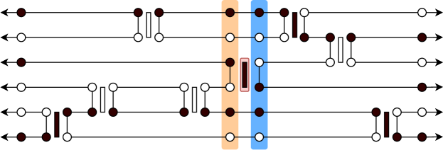
Figure 1: Sketch of SMA excitation spectrum measurement of a six-spin system with Stochastic Series Expansion. The imaginary time dimension is depicted horizontally. Filled and open circles represent $\uparrow$ and $\downarrow$ spins, respectively. Black bonds, which change the spin configuration, denote off-diagonal operators. White bonds that keep the spins unchanged denote diagonal operators. The identity operator is omitted in this figure. The bond highlighted by the red box represents the randomly chosen non-identity operator. “Configuration 1” and “Configuration 2” denote the spin configurations in light orange and blue boxes, respectively. Here, “Configuration 1” is $|\uparrow\downarrow\uparrow\downarrow\uparrow\downarrow\rangle$ and “Configuration 2” is $|\uparrow\downarrow\downarrow\uparrow\uparrow\downarrow\rangle$.

As far as we know, SMA has yet to be used in the QMC simulations. In this paper, we develop an efficient scheme combining the SMA into QMC algorithms to extract the dispersion information with cheap cost and low barrier of technique. This new approach can reach large spin systems with up to $10^{6}$ spins.

This paper is organized as follows: We begin in Sec. II by introducing the Single-Mode Approximation. In Sec. III, we describe how the SSE algorithm cooperates with SMA. In Sec. IV, we discuss how SMA works with the projector QMC method on a valence-bond (VB) basis. We show the results of several calculations in Sec. V and conclude with a summary in Sec. VI.

II Single-Mode Approximation

The key point of SMA is the assumption that the dynamical structure factor of the system consists of a single excitation created by acting some momentum-dependent operators on the ground state. An appropriate trial operator produces a well-estimated upper bound of the low-energy excitation [41]. In this paper, spin models are taken as examples for demonstration. For convenience, We choose the $S^{z}$ operator in momentum space as the form of excitation:

$$S^{z}(\boldsymbol{q})=\frac{1}{\sqrt{N}}\sum_{i}e^{-i\boldsymbol{q}\cdot\boldsymbol{r}_{i}}S^{z}_{i},$$ (1)

where $\boldsymbol{q}$ is a given momentum. $S_{z}(i)$ denotes the $z$ component of the spin at site $i$. The corresponding dynamical structure factor is

$$S_{z}^{2}(\boldsymbol{q})=\langle\mathrm{GS}|S^{z{\dagger}}(\boldsymbol{q})S^{z}(\boldsymbol{q})|\mathrm{GS}\rangle.$$ (2)

By using these notations, the single-mode approximation spectrum can be expressed as

$$\omega\leq\omega_{\mathrm{SMA}}=\frac{1}{2}\frac{\langle\mathrm{GS}|[S^{z}(-\boldsymbol{q}),[H,S^{z}(\boldsymbol{q})]]|\mathrm{GS}\rangle}{S_{z}^{2}(\boldsymbol{q})},$$ (3)

where $\omega_{\mathrm{SMA}}$ is an upper bound of energy gap at wavevector $\boldsymbol{q}$ [37, 38, 39, 40, 41].

Under some circumstances, after the trial momentum-dependent operator is applied to the ground state, the state we get,

$$|\boldsymbol{S}_{\boldsymbol{q}}\rangle\equiv\boldsymbol{S}_{\boldsymbol{q}}|\mathrm{GS}\rangle,$$ (4)

is not orthogonal to the ground state $|\mathrm{GS}\rangle$. That is

$$\langle\mathrm{GS}|\boldsymbol{S}_{\boldsymbol{q}}\rangle\neq 0.$$ (5)

In such cases, to get an estimate of the dispersion, one has to orthogonalize $|\boldsymbol{S}_{\boldsymbol{q}}\rangle$ to $|\mathrm{GS}\rangle$ by a Gram-Schmidt step first:

$$|\boldsymbol{S}_{\boldsymbol{q}}\rangle_{\mathrm{o}}=|\boldsymbol{S}_{\boldsymbol{q}}\rangle-\frac{\langle\mathrm{GS}|\boldsymbol{S}_{\boldsymbol{q}}\rangle}{\langle\mathrm{GS}|\mathrm{GS}\rangle}|\mathrm{GS}\rangle.$$ (6)

After replacing $|\boldsymbol{S}_{\boldsymbol{q}}\rangle$ by $|\boldsymbol{S}_{\boldsymbol{q}}\rangle_{\mathrm{o}}$ in the dynamical structure factor, the Single-Mode Approximation expression is now

$$\omega_{\mathrm{SMA}}=\frac{1}{2}\frac{\langle\mathrm{GS}|[S^{z}(-\boldsymbol{q}),[H,S^{z}(\boldsymbol{q})]]|\mathrm{GS}\rangle}{S_{z}^{2}(\boldsymbol{q})-\frac{|\langle\mathrm{GS}|\boldsymbol{S}_{\boldsymbol{q}}|\mathrm{GS}\rangle|^{2}}{\langle\mathrm{GS}|\mathrm{GS}\rangle}}.$$ (7)

III SMA combined with SSE

This section introduces how to perform SMA calculations with SSE and explains how the measurements are performed.

The stochastic series expansion  [2, 3, 4, 7, 8] approach constitutes a method to simulate sign-problem-free spin systems using quantum Monte Carlo techniques. Here, we briefly summarize the important part of this algorithm. Its starting point is the partition function of the system:

$$Z=\mathrm{Tr}(e^{-\beta H}).$$ (8)

Its Taylor expansion replaces the exponential operator in the partition function, and the trace is rewritten as a summation over a complete basis of the system,

$$Z=\sum_{\alpha}\sum_{n=0}^{\infty}\frac{\beta^{n}}{n!}\langle\alpha|(-H)^{n}|\alpha\rangle$$ (9)

The Hamiltonian is written as the sum of several terms

$$H=\sum_{i}H_{i}$$ (10)

where $i$ is a label for enumerating different terms. The Taylor series is truncated at $M$. $M$ should be sufficiently large so that the truncation error is small enough and negligible. After all these steps, the partition function is

$$Z=\sum_{\alpha}\sum_{\{H_{a}\}}\frac{\beta^{n}(M-n)!}{M!}\langle\alpha|\prod_{i}H_{a_{i}}|\alpha\rangle$$ (11)

All possible operator strings with lengths between 0 and $M$ are summed over. $\alpha$ and $H_{a}$ are sampled during a Monte Carlo procedure according to each term’s weight.

Since the SSE is usually performed in spin $S_{Z}$ basis, the dynamical structure factor of the spin z component in Eq.(2), i.e., the denominator part of Eq.(16), can be directly measured. The double commutator, i.e., the numerator part of Eq.(16), can be measured as follows. It contains four terms,

$$\frac{1}{2}\langle\hat{S}_{\boldsymbol{q}}^{z{\dagger}}\hat{H}\hat{S}_{\boldsymbol{q}}^{z}-\hat{S}_{\boldsymbol{q}}^{z{\dagger}}\hat{S}_{\boldsymbol{q}}^{z}\hat{H}-\hat{H}\hat{S}_{\boldsymbol{q}}^{z}\hat{S}_{\boldsymbol{q}}^{z{\dagger}}+\hat{S}_{\boldsymbol{q}}^{z}\hat{H}\hat{S}_{\boldsymbol{q}}^{z{\dagger}}\rangle.$$ (12)

We use hat to distinguish operators from numbers in this section.

We now briefly describe how to measure these quantities from SMA. After the system has reached equilibrium (ground state in this case), randomly choose a non-identity operator from imaginary time. For convenience, we assume the imaginary time dimension is horizontal, as shown in Fig.1. “Configuration 1/2” denotes the state (or spin configuration) on the left/right side of the chosen operator, respectively. Notice that $\hat{S}_{\boldsymbol{q}}^{z}$ is diagonal (although not Hermitian in most cases) in $S_{z}$ basis, so these $\hat{S}_{\boldsymbol{q}}^{z}$ and $\hat{S}_{\boldsymbol{q}}^{z{\dagger}}$ operators beside $\hat{H}$ can be applied on “Configuration 1” or “Configuration 2” and become a complex number. We abbreviate them to “C1” and “C2” below. For example,

$$\langle\hat{S}_{\boldsymbol{q}}^{z{\dagger}}\hat{H}\hat{S}_{\boldsymbol{q}}^{z}\rangle =\langle S_{\boldsymbol{q}}^{z*}(\mathrm{C1})S_{\boldsymbol{q}}^{z}(\mathrm{C2})\hat{H}\rangle$$ (13)

$$=\langle S_{\boldsymbol{q}}^{z*}(\mathrm{C1})S_{\boldsymbol{q}}^{z}(\mathrm{C2})\frac{\hat{n}}{\beta}\rangle$$

In second line, $\hat{H}$ is replaced by $\hat{n}/\beta$, which is the trick of energy estimator in SSE algorithm [3, 7]. Making use of the relation Eq.(13), the double commutator estimator can be expressed as

$$f(\boldsymbol{q})=\frac{1}{2}\langle( S_{\boldsymbol{q}}^{z*}(\mathrm{C1})S_{\boldsymbol{q}}^{z}(\mathrm{C2})+S_{\boldsymbol{q}}^{z*}(\mathrm{C1})S_{\boldsymbol{q}}^{z}(\mathrm{C1})$$ (14)

$$+S_{\boldsymbol{q}}^{z}(\mathrm{C2})S_{\boldsymbol{q}}^{z*}(\mathrm{C2})+S_{\boldsymbol{q}}^{z}(\mathrm{C1})S_{\boldsymbol{q}}^{z*}(\mathrm{C2}))\times\frac{\hat{n}}{\beta}\rangle,$$

which is the final expression of the SMA spectrum. This expression is independent of forms of Hamiltonians, enabling us to use SMA in systems with complicated Hamiltonians.

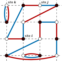
Figure 2: Illustration of a valence-bond transposition graph on a $4\times 4$ square lattice. Solid circles represent sites on sublattice A, and open circles represent sites on sublattice B. Red and blue bond configuration represent the bra $\langle\psi_{\mathrm{L}}|$ and the ket $|\psi_{\mathrm{R}}\rangle$ respectively. This figure is a transposition graph of the inner product $\langle\psi_{\mathrm{L}}|\psi_{\mathrm{R}}\rangle$. Spins on site $i$ and $j$ belong to the same loop, so $\langle\psi_{\mathrm{L}}|\boldsymbol{S}_{i}\cdot\boldsymbol{S}_{j}|\psi_{\mathrm{R}}\rangle/\langle\psi_{\mathrm{L}}|\psi_{\mathrm{R}}\rangle=-3/4$. Spins on-site $i$ and $k$ are not correlated since they are in different loops.

IV SMA combined with projector QMC

The Projector QMC method was initially introduced by Sandvik [42, 43] to access ground states of quantum spin systems efficiently. This algorithm is formulated in a combined space of spin $S_{z}$ and valence-bond bases. Since one can directly obtain information on valence bonds, it is naturally suited for studying spin rotationally-invariant Hamiltonians, such as the Heisenberg model and its extension versions with long-range interactions. The properties of valence-bond basis and projector QMC methods have been demonstrated in detail in the literature [42, 43, 44].

In this section, we describe our algorithm with the Heisenberg model

$$H=\sum_{i,j}J_{ij}\boldsymbol{S}_{i}\cdot\boldsymbol{S}_{j}..$$ (15)

Hamiltonian containing only Heisenberg interactions can be simulated efficiently using the below-mentioned method.

Based on the definition of SMA spectrum, we define

$$f(\boldsymbol{q})=\frac{1}{2}\langle\mathrm{GS}|[\boldsymbol{S}(-\boldsymbol{q}),[H,\boldsymbol{S}(\boldsymbol{q})]]|\mathrm{GS}\rangle,$$ (16)

where $\boldsymbol{S}(\boldsymbol{q})$ denotes the Fourier transform of spin operator

$$\boldsymbol{S}(\boldsymbol{q})=\frac{1}{\sqrt{N}}\sum_{i}e^{-i\boldsymbol{q}\cdot\boldsymbol{r}_{i}}\boldsymbol{S}_{i}.$$ (17)

After we expanding Eq.(16) with Eq.(17) and Hamiltonian Eq.(15), $f(\boldsymbol{q})$ is written as

$$f(\boldsymbol{q})=\frac{1}{2N} \sum_{i,j}J_{ij}\sum_{l,l^{\prime}}e^{-i\boldsymbol{q}\cdot(\boldsymbol{r}_{l}-\boldsymbol{r}_{l^{\prime}})}$$ (18)

$$\langle\mathrm{GS}|[\boldsymbol{S}_{l^{\prime}},[\boldsymbol{S}_{i}\cdot\boldsymbol{S}_{j},\boldsymbol{S}_{l}]]|\mathrm{GS}\rangle.$$

Only terms of which both subscripts $l$ and $l^{\prime}$ take values $i$ or $j$ are non-zero since operators on different sites commute with each other. Commutation relations [45]

$$[\boldsymbol{S}_{i},[\boldsymbol{S}_{i}\cdot\boldsymbol{S}_{j},\boldsymbol{S}_{i}]]=2\boldsymbol{S}_{i}\cdot\boldsymbol{S}_{j},$$ (19)

$$[\boldsymbol{S}_{i},[\boldsymbol{S}_{i}\cdot\boldsymbol{S}_{j},\boldsymbol{S}_{j}]]=-2\boldsymbol{S}_{i}\cdot\boldsymbol{S}_{j},$$ (20)

can be obtained after some simple $\mathrm{SU}(2)$ algebra calculations. Taking all of these relations into account, we finally get

$$f(\boldsymbol{q})=-\frac{4}{N}\sum_{i,j}J_{ij}\sin^{2}(\frac{1}{2}\boldsymbol{q}\cdot(\boldsymbol{r}_{i}-\boldsymbol{r}_{j}))\langle\boldsymbol{S}_{i}\cdot\boldsymbol{S}_{j}\rangle_{\mathrm{GS}}.$$ (21)

Here we have replaced $\langle\mathrm{GS}|\boldsymbol{S}_{i}\cdot\boldsymbol{S}_{j}|\mathrm{GS}\rangle$ by its abbreviation $\langle\boldsymbol{S}_{i}\cdot\boldsymbol{S}_{j}\rangle_{\mathrm{GS}}$. Spin-spin correlation in the ground state can be easily estimated in VB basis [44]:

$$\langle\boldsymbol{S}_{i}\cdot\boldsymbol{S}_{j}\rangle_{\mathrm{GS}}=\frac{3}{4}\epsilon_{ij}\delta^{ij}.$$ (22)

Here $\epsilon_{ij}$ is -1 if site $i$ and $j$ are on the same sub-lattice of underlying bipartite lattice, and is one otherwise. $\delta^{ij}$ equals one if site $i$ and $j$ belong to the same loop formed in the transposition graph. If they belong to different loops, then $\delta^{ij}$ takes the value of 0. See Fig.2 as an example.

To obtain the SMA spectrum of the Heisenberg model, only spin-spin correlations in the ground state are necessary. Projector QMC and VB basis offer quick and convenient access to these correlation functions. Non-trivial parallel programming can be applied to this algorithm, remarkably enhancing power and efficiency. These advantages enable us to obtain a spectrum of systems with $10^{4}$, even $10^{5}$ spins.

Although the spectrum of some simple Hamiltonians, like the Heisenberg model, can be simulated and obtained easily, the method discussed in this section could be more suitable for systems with complicated Hamiltonians. Trying to simplify the double commutator may eventually obtain observables that are hard to estimate in practice. For example, Q term interaction $(\boldsymbol{S}_{i}\cdot\boldsymbol{S}_{j})(\boldsymbol{S}_{k}\cdot\boldsymbol{S}_{l})$ in J-Q model  [46, 47, 48] produce terms including

$$[S^{z}_{i},[(\boldsymbol{S}_{i}\cdot\boldsymbol{S}_{j})(\boldsymbol{S}_{k}\cdot\boldsymbol{S}_{l}),S^{z}_{k}]]=-\frac{1}{3}(\boldsymbol{S}_{i}\times\boldsymbol{S}_{j})\cdot(\boldsymbol{S}_{k}\times\boldsymbol{S}_{l}).$$ (23)

In principle, cross-product terms can be estimated using QMC. However, the procedure would be cumbersome since cross-product terms contain several off-diagonal operators. Thus, whenever the simplified expression of the double commutator is not easy to measure, the algorithm introduced in Sec. II should be applied instead.

The following section will show several examples calculated using the methods mentioned above.

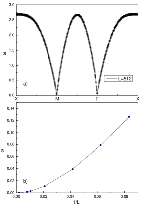
Figure 3: a) SMA spectrum of 2D AFM Heisenberg model on a square lattice of system size $L=512$. Periodic boundary condition is applied. Two gapless excitation modes exist at $M$ and $\Gamma$ points, respectively. b) Energy excitation gap at $M$ point of different system sizes. With the increase in system size, the gap at $M$ converges to zero. Errors of data are smaller than the symbol sizes.

V Results

V.1 2D AFM Heisenberg Model

The first case is the two-dimensional antiferromagnetic (AFM) Heisenberg model with only nearest neighbor interactions on a square lattice

$$H=J\sum_{\langle i,j\rangle}\boldsymbol{S}_{i}\cdot\boldsymbol{S}_{j}$$ (24)

where $\langle i,j\rangle$ denotes nearest neighbor sites, and coupling $J>0$.

This Hamiltonian is simple, so we calculate using projector QMC with non-trivial parallel programming. Systems with $512\times 512$ spins are simulated, and the SMA spectrum obtained is shown in Fig.3 (a). Two gapless modes exist, one at $M$ point of momentum space and the other at $\Gamma$ point. Both gapless modes have linear dispersion in the low-energy part. This result is consistent with the spectrum given by spin-wave theory [49].

It is worth noting here that indicated by the original SMA expression Eq.(3), either the double commutator vanishes or the dynamical structure factor diverges as a function of system size would induce the absence of an energy gap.

At $\Gamma$ point, the operator acted on the system commutes with the total Hamiltonian,

$$[S_{z}(\boldsymbol{q}=0),J\sum_{\langle i,j\rangle}\boldsymbol{S}_{i}\cdot\boldsymbol{S}_{j}]=0.$$ (25)

As a result, the numerator is always zero, regardless of the system size.

At the $M$ point, the dynamical structure factor on the denominator increases with system size and finally diverges in the thermal-dynamic limit. This fact indicates that there must be a gapless mode at $M$. As shown in Fig.3 (b), the energy gap becomes smaller and converges to zero with the increase of lattice size.

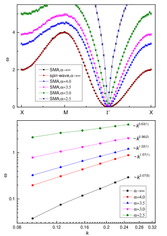
Figure 4: The upper panel is the SMA spectrum and spin-wave theory spectrum of the 2D ferromagnetic Heisenberg model on a square lattice. Lattice size $L=48$. Periodic boundary condition is applied. Only interactions between nearest neighbors are included when power exponent $\alpha$ approaches infinity. Different $\alpha$ leads to different dispersion relation near $\Gamma$. The lower panel is the dispersion relations near the $\Gamma$ point. Power law fitting results are labeled on the panel. The dispersion power exponent decreases with decreasing $\alpha$. Error bars are smaller than the size of the symbol.

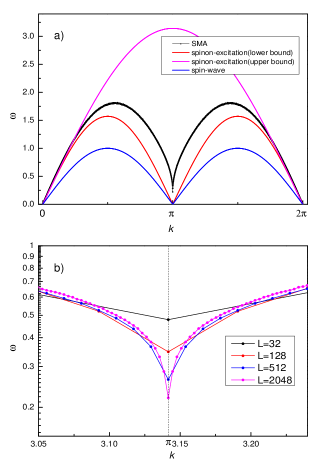
Figure 5: a) The black line shows the SMA spectrum of the anti-ferromagnetic Heisenberg chain. The lower and upper bounds of spinon excitation are shown with red and purple lines, respectively. The blue line indicates the result of the spin-wave theory (which is wrong). The length of the chain is $L=2048$. b) Energy gap near momentum $\pi$ of different chain length. Maximum chain length $L=2048$ is reached. In both figures, error bars are smaller than the symbols.

V.2 2D long-range FM Heisenberg Model

The next example is the two-dimensional ferromagnetic (FM) Heisenberg model with long-range interactions. The Hamiltonian is

$$H=\sum_{i,j}J_{ij}\boldsymbol{S}_{i}\cdot\boldsymbol{S}_{j}$$ (26)

with $J_{ij}<0$. Here, the term “long-range” means that the coupling strength decays as a power law form:

$$H=\sum_{i,j}\frac{1}{|r_{ij}|^{\alpha}}\boldsymbol{S}_{i}\cdot\boldsymbol{S}_{j}$$ (27)

The power exponent $\alpha$ controls the effective range of coupling. As $\alpha$ approaches infinity, the model returns to the Heisenberg model with only nearest-neighbor interactions. Strong long-distance couplings come in with small $\alpha$. Spectrums of ferromagnetic Heisenberg models can be well estimated by spin wave theory [49, 50, 51]. According to spin-wave theory, the dispersion of a magnon is

$$\omega_{\mathrm{FM}}(\boldsymbol{q})=|J_{0}-J_{\boldsymbol{q}}|$$ (28)

where $J_{\boldsymbol{q}}$ is the Fourier transform of $J_{ij}$

$$J_{\boldsymbol{q}}=\sum_{\boldsymbol{r}}e^{-i\boldsymbol{q}\cdot\boldsymbol{r}}J_{\boldsymbol{r}}$$ (29)

Here, we compare our SMA results with the dispersion of magnon. Results are exhibited in Fig.4. Fig.4 (a) shows the spectrum of the Heisenberg model with different decay exponent $\alpha$. When $\alpha$ approaches infinity, only nearest-neighbor interactions are considered. In this case, our result is consistent with the spectrum given by spin-wave theory. The corresponding dispersion near the $\Gamma$ point is quadratic. As is shown in Fig.4, as $\alpha$ decreases to $2.5$, this gapless mode still retains. However, the dispersion relations

$$\omega\sim k^{s}$$ (30)

varies with $\alpha$. In the nearest neighbor version, dispersion power exponent $s=2$. As $\alpha$ decreases, $s$ also decreases. This mode has a linear dispersion when $\alpha=3.0$. Corresponding $s$ has been tagged on the lower panel of Fig.4. All results are well compatible with magnon dispersion given by spin-wave theory for long-range interactions [49, 51].

V.3 AFM Heisenberg Chain

If the SMA algorithm always gives the same spectrum as spin-wave theory, undoubtedly, it makes this method less appealing. Fortunately, this is not the case.

The last case shown in this paper is an anti-ferromagnetic Heisenberg chain with periodic boundary conditions. The Hamiltonian is

$$H=J\sum_{i=1}^{N}\boldsymbol{S}_{i}\cdot\boldsymbol{S}_{i+1}$$ (31)

where $\boldsymbol{S}_{N+1}=\boldsymbol{S}_{1}$ and $J>0$.

As is known, spin wave theory breaks down here and gives a wrong dispersion velocity [52]

$$v_{\mathrm{SW}}=|J|$$ (32)

which is shown in Fig.5 with the blue line. This velocity is smaller than the correct result obtained from spinon theory [52]

$$v_{\mathbf{magnon}}=\frac{\pi}{2}|J|.$$ (33)

As shown in Fig.5, we can obtain the correct velocity near momentum $0$ and $2\pi$ from SMA calculations. In this case, SMA still works while spin-wave theory breaks down, indicating SMA calculation’s better feasibility.

At momentum $\pi$, according to spinon excitation, there exists a strongly continuous spectrum [52]. In such cases, SMA’s upper bound energy gap estimation is unreliable. With the increase of the system size, the gap given by SMA becomes smaller (Fig.5 b)). With the chain length increase, this gap converges to zero as the system approaches the thermodynamic limit. However, SMA does not tell the correct velocity of dispersion near momentum $\pi$ because of the continuous spectrum.

VI Conclusions

We introduce an algorithm to perform single-mode approximation calculations via quantum Monte Carlo. In particular, two versions of the combination of single-mode approximation with quantum Monte Carlo are employed. Projector QMC with non-trivial parallel programming can be applied when directly simplifying the double commutator. In this case, large systems with $10^{6}$ spins are accessible. For a system with a complicated Hamiltonian, we develop another general method with which forms of the Hamiltonians become irrelevant. Both algorithms can perform large-scale simulations outside of the reach of conventional spectrum-estimating algorithms. They may play an important role when large system sizes are crucial in exhibiting exotic excitations, and many systems should be selected according to their excitations. Several cases are calculated as examples. In the two-dimensional Heisenberg model, either ferromagnetic or anti-ferromagnetic, SMA calculations give the correct excitation dispersions consistent with spin-wave theory. In the 1D anti-ferromagnetic chain, SMA goes beyond the spin-wave theory. Although the approximation near continuous spectrum could be more accurate, the correct velocity of dispersion near momentum 0 and $2\pi$ can be obtained. With the advent of this state-of-the-art algorithm, scanning through parameters and performing statistical works of the spectrum have become possible.

VII Acknowledgements

This work is supported by the National Key Research and Development Program of China Grant No. 2022YFA1404204, and the National Natural Science Foundation of China Grant No. 12274086. ZY thanks the inspirational discussions with Zi Yang Meng, Amos Chan, and David Huse in another related project and the support from the start-up funding of Westlake University and the open fund of Lanzhou Center for Theoretical Physics (12247101). Y.C.W. acknowledges the support from Zhejiang Provincial Natural Science Foundation of China (Grant No. LZ23A040003), and the support from the High-performance Computing Centre of Zhongfa Aviation Institute of Beihang University. The authors acknowledge the Beijing PARATERA Tech Co., Ltd. for providing HPC resources that have contributed to the research results reported within this paper.

References

- Gubernatis et al. [2016] J. Gubernatis, N. Kawashima, and P. Werner, Quantum Monte Carlo Methods (Cambridge University Press, 2016).
- Sandvik and Kurkijärvi [1991] A. W. Sandvik and J. Kurkijärvi, Quantum monte carlo simulation method for spin systems, Phys. Rev. B 43, 5950 (1991).
- Sandvik [1999] A. W. Sandvik, Stochastic series expansion method with operator-loop update, Phys. Rev. B 59, R14157 (1999).
- Syljuåsen and Sandvik [2002] O. F. Syljuåsen and A. W. Sandvik, Quantum monte carlo with directed loops, Phys. Rev. E 66, 046701 (2002).
- Yan et al. [2019] Z. Yan, Y. Wu, C. Liu, O. F. Syljuåsen, J. Lou, and Y. Chen, Sweeping cluster algorithm for quantum spin systems with strong geometric restrictions, Phys. Rev. B 99, 165135 (2019).
- Yan [2022] Z. Yan, Global scheme of sweeping cluster algorithm to sample among topological sectors, Phys. Rev. B 105, 184432 (2022).
- Sandvik [2019] A. W. Sandvik, Stochastic series expansion methods (2019), arXiv:1909.10591 [cond-mat.str-el] .
- Desai and Pujari [2021] N. Desai and S. Pujari, Resummation-based quantum monte carlo for quantum paramagnetic phases, Phys. Rev. B 104, L060406 (2021).
- Prokof’ev et al. [1998] N. Prokof’ev, B. Svistunov, and I. Tupitsyn, “worm” algorithm in quantum monte carlo simulations, Phys. Lett. A 238, 253 (1998).
- Boninsegni et al. [2006a] M. Boninsegni, N. V. Prokof’ev, and B. V. Svistunov, Worm algorithm and diagrammatic monte carlo: A new approach to continuous-space path integral monte carlo simulations, Phys. Rev. E 74, 036701 (2006a).
- Boninsegni et al. [2006b] M. Boninsegni, N. Prokof’ev, and B. Svistunov, Worm algorithm for continuous-space path integral monte carlo simulations, Phys. Rev. Lett. 96, 070601 (2006b).
- Krzakala et al. [2008] F. Krzakala, A. Rosso, G. Semerjian, and F. Zamponi, Path-integral representation for quantum spin models: Application to the quantum cavity method and monte carlo simulations, Phys. Rev. B 78, 134428 (2008).
- Kosztin et al. [1996] I. Kosztin, B. Faber, and K. Schulten, Introduction to the diffusion Monte Carlo method, American Journal of Physics 64, 633 (1996).
- Syljuåsen [2005a] O. F. Syljuåsen, Diffusion monte carlo in continuous time, Journal of low temperature physics 140, 281 (2005a).
- Syljuåsen [2005b] O. F. Syljuåsen, Random walks near rokhsar–kivelson points, International Journal of Modern Physics B 19, 1973 (2005b).
- Syljuåsen [2005] O. F. Syljuåsen, Continuous-time diffusion monte carlo method applied to the quantum dimer model, Phys. Rev. B 71, 020401(R) (2005).
- Syljuåsen [2006] O. F. Syljuåsen, Plaquette phase of the square-lattice quantum dimer model: Quantum monte carlo calculations, Phys. Rev. B 73, 245105 (2006).
- Trivedi and Ceperley [1990] N. Trivedi and D. M. Ceperley, Ground-state correlations of quantum antiferromagnets: A green-function monte carlo study, Phys. Rev. B 41, 4552 (1990).
- Trivedi and Ceperley [1989] N. Trivedi and D. M. Ceperley, Green-function monte carlo study of quantum antiferromagnets, Phys. Rev. B 40, 2737 (1989).
- Arnow et al. [1982] D. M. Arnow, M. H. Kalos, M. A. Lee, and K. E. Schmidt, Green’s function monte carlo for few fermion problems, The Journal of Chemical Physics 77, 5562 (1982).
- Lee and Schmidt [1992] M. A. Lee and K. E. Schmidt, Green’s function monte carlo, Computer in Physics 6, 192 (1992).
- Gull and Skilling [1984] S. Gull and J. Skilling, Maximum entropy method in image processing, IEE Proceedings F (Communications, Radar and Signal Processing) 131, 646 (1984).
- Sandvik [1998] A. W. Sandvik, Stochastic method for analytic continuation of quantum monte carlo data, Phys. Rev. B 57, 10287 (1998).
- Beach [2004] K. S. D. Beach, Identifying the maximum entropy method as a special limit of stochastic analytic continuation (2004), arXiv:cond-mat/0403055 [cond-mat.str-el] .
- Syljuåsen [2008] O. F. Syljuåsen, Using the average spectrum method to extract dynamics from quantum monte carlo simulations, Phys. Rev. B 78, 174429 (2008).
- Sandvik [2016] A. W. Sandvik, Constrained sampling method for analytic continuation, Phys. Rev. E 94, 063308 (2016).
- Shao and Sandvik [2023] H. Shao and A. W. Sandvik, Progress on stochastic analytic continuation of quantum monte carlo data, Physics Reports 1003, 1 (2023).
- Yan et al. [2022a] Z. Yan, X. Ran, Y.-C. Wang, R. Samajdar, J. Rong, S. Sachdev, Y. Qi, and Z. Y. Meng, Fully packed quantum loop model on the triangular lattice: Hidden vison plaquette phase and cubic phase transitions, arXiv preprint arXiv:2205.04472 (2022a).
- Yan et al. [2021] Z. Yan, Y.-C. Wang, N. Ma, Y. Qi, and Z. Y. Meng, Topological phase transition and single/multi anyon dynamics of z 2 spin liquid, npj Quantum Materials 6, 39 (2021).
- Wang et al. [2021] Y.-C. Wang, Z. Yan, C. Wang, Y. Qi, and Z. Y. Meng, Vestigial anyon condensation in kagome quantum spin liquids, Phys. Rev. B 103, 014408 (2021).
- Wang et al. [2018] Y.-C. Wang, X.-F. Zhang, F. Pollmann, M. Cheng, and Z. Y. Meng, Quantum Spin Liquid with Even Ising Gauge Field Structure on Kagome Lattice, Phys. Rev. Lett. 121, 057202 (2018).
- Zhou et al. [2021] C. Zhou, Z. Yan, H.-Q. Wu, K. Sun, O. A. Starykh, and Z. Y. Meng, Amplitude mode in quantum magnets via dimensional crossover, Phys. Rev. Lett. 126, 227201 (2021).
- Yan et al. [2022b] Z. Yan, R. Samajdar, Y.-C. Wang, S. Sachdev, and Z. Y. Meng, Triangular lattice quantum dimer model with variable dimer density (2022b), arXiv:2202.11100 [cond-mat.str-el] .
- Zhou et al. [2022] Z. Zhou, C. Liu, Z. Yan, Y. Chen, and X.-F. Zhang, Quantum dynamics of topological strings in a frustrated ising antiferromagnet, npj Quantum Materials 7, 60 (2022).
- Liu et al. [2022] Z. Liu, J. Li, R.-Z. Huang, J. Li, Z. Yan, and D.-X. Yao, Bulk and edge dynamics of a two-dimensional affleck-kennedy-lieb-tasaki model, Phys. Rev. B 105, 014418 (2022).
- Yan and Meng [2023] Z. Yan and Z. Y. Meng, Unlocking the general relationship between energy and entanglement spectra via the wormhole effect, Nature Communications 14, 2360 (2023).
- Yi et al. [2002] S. Yi, Ö. E. Müstecaplıoğlu, C.-P. Sun, and L. You, Single-mode approximation in a spinor-1 atomic condensate, Physical Review A 66, 011601(R) (2002).
- Bruschi et al. [2010] D. E. Bruschi, J. Louko, E. Martín-Martínez, A. Dragan, and I. Fuentes, Unruh effect in quantum information beyond the single-mode approximation, Physical Review A 82, 042332 (2010).
- Läuchli et al. [2008] A. M. Läuchli, S. Capponi, and F. F. Assaad, Dynamical dimer correlations at bipartite and non-bipartite rokhsar–kivelson points, Journal of Statistical Mechanics: Theory and Experiment 2008, P01010 (2008).
- Yan et al. [2022c] Z. Yan, Z. Y. Meng, D. A. Huse, and A. Chan, Height-conserving quantum dimer models, arXiv preprint arXiv:2204.01740 (2022c).
- Lauchli et al. [2008] A. M. Lauchli, S. Capponi, and F. F. Assaad, Dynamical dimer correlations at bipartite and non-bipartite rokhsar-kivelson points, Journal of Statistical Mechanics: Theory and Experiment 10, 1742 (2008).
- Sandvik [2005] A. W. Sandvik, Ground state projection of quantum spin systems in the valence-bond basis, Phys. Rev. Lett. 95, 207203 (2005).
- Sandvik and Evertz [2010] A. W. Sandvik and H. G. Evertz, Loop updates for variational and projector quantum monte carlo simulations in the valence-bond basis, Phys. Rev. B 82, 024407 (2010).
- Beach and Sandvik [2006] K. Beach and A. W. Sandvik, Some formal results for the valence bond basis, Nucl. Phys. B 750, 142 (2006).
- Vörös and Penc [2021] D. Vörös and K. Penc, Dynamical structure factor of the su(3) heisenberg chain: Variational monte carlo approach, Phys. Rev. B 104, 184426 (2021).
- Sandvik [2007] A. W. Sandvik, Evidence for deconfined quantum criticality in a two-dimensional heisenberg model with four-spin interactions, Phys. Rev. Lett. 98, 227202 (2007).
- Sandvik [2010] A. W. Sandvik, Continuous quantum phase transition between an antiferromagnet and a valence-bond solid in two dimensions: Evidence for logarithmic corrections to scaling, Phys. Rev. Lett. 104, 177201 (2010).
- Pujari et al. [2013] S. Pujari, K. Damle, and F. Alet, Néel-state to valence-bond-solid transition on the honeycomb lattice: Evidence for deconfined criticality, Phys. Rev. Lett. 111, 087203 (2013).
- Song et al. [2023] M. Song, J. Zhao, C. Zhou, and Z. Y. Meng, Dynamical properties of quantum many-body systems with long-range interactions, Phys. Rev. Res. 5, 033046 (2023).
- Defenu et al. [2023] N. Defenu, T. Donner, T. Macrì, G. Pagano, S. Ruffo, and A. Trombettoni, Long-range interacting quantum systems, Rev. Mod. Phys. 95, 035002 (2023).
- Diessel et al. [2023] O. K. Diessel, S. Diehl, N. Defenu, A. Rosch, and A. Chiocchetta, Generalized higgs mechanism in long-range-interacting quantum systems, Phys. Rev. Res. 5, 033038 (2023).
- Takahashi [2005] M. Takahashi, Thermodynamics of One-Dimensional Solvable Models (2005).