The entropy of finite gravitating regions

Abstract

We develop a formalism for calculating the entanglement entropy of an arbitrary spatial region of a gravitating spacetime at a moment of time symmetry. The crucial ingredient is a path integral over embeddings of the region into the overall spacetime, interpretable as a sum over the edge modes associated with the region. We find that the entanglement entropy of a gravitating region equals the minimal surface area among all regions that enclose it. This suggests a notion of “terrestrial holography” where regions of space can encode larger ones, in contrast to the standard form of holography, in which degrees of freedom on the celestial sphere at the boundary of the universe encode the interior.

1 Introduction

Gravity has a deep and mysterious connection to thermodynamics: the entropy of some gravitating systems is geometrized as the area of a distinguished surface in spacetime. For example, black holes appear to carry a coarse-grained entropy of $S=A/4G_{N}$ where $A$ is the area of the horizon and $G_{N}$ is Newton’s constant Bekenstein:1973ur ; hawkingBH . Cosmological Gibbons:1977mu and Rindler Jacobson_2003 ; Unruh:1976db horizons associated to accelerating observers also obey a similar relation, although the statistical interpretation of these entropies remains obscure. Associating an entropy to causal horizons can even be used to derive the Einstein equations Jacobson_1995 . In addition, in the context of the holographic AdS/CFT correspondence, certain extremal surfaces measure entanglement entropy between the quantum degrees of freedom associated to opposite sides of the surface Ryu_2006 ; Faulkner:2013ana ; Hubeny:2007xt ; Engelhardt:2014gca . These relations lead us to ask whether there is a relation between entropy and area for arbitrary subregions of a gravitating spacetime. These relations recently led Bousso and Penington to propose that there is a relation between entropy and area for arbitrary subregions of a gravitating spacetime at a moment of time symmetry BP_static . Here, we will provide evidence in support of this conjecture.

To this end, we propose a path integral for gravity in any finite subregion of a global spacetime which is invariant under diffeomorphisms inside that region. We use this path integral to argue that the entanglement entropy of an open region $a$ at a moment of time symmetry is determined by a (possibly larger) region $E(a)$ defined by: (1) $a\subseteq E(a)$, and (2) $E(a)$ minimizes the generalized entropy among all regions satisfying (1). This argument makes no assumption about the cosmological constant. When the entanglement entropy of the matter fields can be neglected, $E(a)$ will simply be the region of minimal surface area containing $a$. The result also implies the entropy of the de Sitter vacuum vanishes, at least in the absence of external observers.

Three sections follow. In Sec. 2, we review and construct the technical tools needed to define subregions of gravitating spacetimes. We then use these tools to define and renormalize the entropy of such a subregion. In Sec. 3, we propose a gravitational path integral for a finite region of space. This path integral includes an integral over all embeddings of the region into spacetime. We then take a saddlepoint approximation to compute the leading order behavior of the entropy in the small coupling ($G_{N}\to 0$) limit. We conclude in Sec. 4 with a discussion of the interpretations and implications of our entropy formula.

2 The entropy of subregions in gravitating spacetimes

Consider a globally hyperbolic manifold $\mathcal{M}$. Let $\Sigma$ be a Cauchy slice at a moment of time symmetry, and denote by $a$ any open region of $\Sigma$ with $a^{\prime}=\text{int}(\Sigma\setminus a)$ the complement of $a$ in $\Sigma$ minus the boundary of $a$. Also define the co-dimension 1 (co-dimension 2 in spacetime) corner of $a$ as $\partial a:=\bar{a}\cap\bar{a}^{\prime}$ where $\bar{a},\bar{a}^{\prime}$ are the closures of $a,a^{\prime}$. Intuitively, $\partial a$ is the boundary between $a,a^{\prime}$.

Let $\mathcal{H}_{\Sigma}$ be the Hilbert space of quantum gravity and matter defined on $\Sigma$. This theory may or may not be known explicitly. In AdS/CFT, $\mathcal{H}_{\Sigma}$ is isomorphic to the Hilbert space of a CFT in one lower dimension Maldacena_1999 , but in flat or de Sitter spacetimes, less is known about the structure of $\mathcal{H}_{\Sigma}$. In the small Newton constant ($G_{N}$) limit, however, a great deal is known about $\mathcal{H}_{\Sigma}$: it contains perturbative gravitons and matter propagating on curved backgrounds. Take $\ket{\Psi}\in\mathcal{H}_{\Sigma}$ to be a state with a well defined semi-classical description and a background geometry $g^{0}_{\mu\nu}$ in the $G_{N}\to 0$ limit. In this limit, we can define an (approximate) algebra of $\mathcal{A}_{\Sigma}$ of observables which act on $\mathcal{H}_{\Sigma}$ Almheiri_2015 . $A_{\Sigma}$ includes both matter fields and perturbative gravitons $h_{\mu\nu}$ such that the total metric is $g_{\mu\nu}=g^{0}_{\mu\nu}+\sqrt{32\pi G_{N}}h_{\mu\nu}$, with the prefactor chosen to normalize the graviton kinetic term. Furthermore, $\mathcal{H}_{\Sigma}$ has a $\text{Diff}(\Sigma)$ diffeomorphism gauge symmetry which corresponds to coordinate changes of the perturbative fields defined on $\Sigma$. In the language of AdS/CFT, the subspace spanned by $\mathcal{A}_{\Sigma}$ acting on $\ket{\Psi}$ defines a code subspace within the full non-perturbative Hilbert space $\mathcal{H}_{\Sigma}$ Almheiri_2015 . Our goal is to compute the entropy of the reduced density matrix $\rho_{a}\sim\tr_{a^{\prime}}\outerproduct{\Psi}{\Psi}$, associated with a bulk region $a$, in the weak coupling $G_{N}\to 0$ limit. A precondition for this reduced state $\rho_{a}$ to be well defined is the existence of a bi-partition of the Hilbert space into $\mathcal{H}_{\Sigma}\sim\mathcal{H}_{a}\otimes\mathcal{H}_{a^{\prime}}$. However, this factorization is subtle in quantum gravity for two distinct reasons.

First, there are UV divergences in the effective field theory (EFT) that we are considering, associated with the sharp cut $\partial a$ between $a,a^{\prime}$ Haag:1992hx . We expect these divergences to be cured in the high energy completion defining $\mathcal{H}_{\Sigma}$ in something like string theory. RG-flow from this complete theory leads to our EFT below a cutoff. With this is mind, we will assume that an appropriate regularization and renormalization makes the path integral that we will consider well defined. Second, if there is a gauge symmetry in the theory, constraints can correlate $a$ and $a^{\prime}$ . This is even true for $U(1)$ lattice gauge theory Donnelly_2012 . We review this lack of factorization in the next two sections, following the discussions in Casini_2014 ; Donnelly_2012 ; Donnelly_2016 .

2.1 Edge modes in lattice gauge theory

Consider a $U(1)$ lattice gauge theory, which manifestly has no UV divergences, and let $\mathcal{H}_{\Sigma}$ be the gauge invariant Hilbert space of the full lattice. As in the continuum, we separate the lattice into a subset of nodes $a$ and its complement $a^{\prime}$, with $\partial a$ cutting the links between them.

Suppose a Wilson line straddles the corner $\partial a$, as in Fig. 1. Then tracing out $a^{\prime}$ will leave behind an open Wilson line with endpoints on $\partial a$. From the perspective of $a$, the endpoints at the cut will carry charges transforming in some representation of the gauge group at $\partial a$. Since the original Hilbert space was gauge invariant, these open Wilson lines constitute new degrees of freedom called “edge modes”. The edge modes are crucial in computations of entanglement entropy in gauge theories Donnelly_2012 . Indeed, the total Hilbert space describing the degrees of freedom on $a$ is the “extended Hilbert space” $\widetilde{\mathcal{H}}_{a}=\mathcal{H}_{a}\otimes\mathcal{H}_{e.m.}$, where $\mathcal{H}_{a}$ has support only inside $a$, and $\mathcal{H}_{e.m.}$ is the edge mode Hilbert space supported on the corner.

To explain how to recover the original Hilbert space, we must first understand the extended Hilbert space. The total gauge symmetry of the lattice $\Sigma$ is $U(1)_{\Sigma}$, i.e., $U(1)$ transformations at every link on the lattice. This gauge group splits as

$$U(1)_{\Sigma}=U(1)_{a}\oplus U(1)_{\partial a}\oplus U(1)_{a^{\prime}}\,,$$ (1)

where $U(1)_{\partial a}$ are gauge transformations transforming links along the cut, while $U(1)_{a}$ consists of gauge transformations of links with both endpoints in $a$ (and similarly for $U(1)_{a^{\prime}}$). The extended Hilbert space $\widetilde{\mathcal{H}}_{a}$ has a gauge symmetry $U(1)_{a}$ that it inherits from $\mathcal{H}_{a}$, and a global symmetry $U(1)_{\partial a}$ acting on $\mathcal{H}_{e.m.}$. The latter is a global symmetry because the open Wilson lines transform in a non-trivial representation of $U(1)_{\partial a}$. In fact, a more careful consideration shows that $\mathcal{H}_{e.m.}\cong L^{2}(U(1)_{\partial a})$. This makes the global symmetry more transparent: it is simply the regular representation of $U(1)_{\partial a}$ on $L^{2}(U(1)_{\partial a})$. We can reason similarly about $\widetilde{\mathcal{H}}_{a^{\prime}}$.

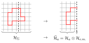
Figure 1: The full Hilbert space $\mathcal{H}_{\Sigma}$ is defined on the complete lattice. When restricting to a subset $a$ of the nodes on the lattice, described by a reduced Hilbert space $\mathcal{H}_{a}$, one must also include additional degrees of freedom to account for the endpoints of Wilson lines not present in $\mathcal{H}_{\Sigma}$. These new degrees of freedom are the edge modes in $\mathcal{H}_{e.m.}$.

Because the extended Hilbert space has a global symmetry $U(1)_{\partial a}$, it splits into superselection sectors of charge eigenstates. The representations of $U(1)_{\partial a}$ are given by $\vec{Q}$, a choice of $U(1)$ charge for every link on the cut, and so $\widetilde{\mathcal{H}}_{a}=\oplus_{\vec{Q}}\widetilde{\mathcal{H}}_{\vec{Q},a}$. Thus, the most general density matrix in $\widetilde{\mathcal{H}}_{a}$ takes the form $\rho_{a}=\sum_{\vec{Q}}p_{\vec{Q}}\rho_{\vec{Q}}$, where $\sum_{\vec{Q}}p_{\vec{Q}}=1$ and each charge-sector density matrix has unit trace. $\rho_{\vec{Q}}$ is any state compatible with the boundary representation. For example, $\rho_{0}$ is a possibly mixed state over Wilson loops which do not touch the boundary. We will return to the implications of this splitting below.

Let us now consider how to recover the original Hilbert space $\mathcal{H}_{\Sigma}$. First, note that $\mathcal{H}_{a}\otimes\mathcal{H}_{a^{\prime}}\subset\mathcal{H}$ because $\mathcal{H}_{a}\otimes\mathcal{H}_{a^{\prime}}$ contains no Wilson lines straddling the cut ${\partial a}$. This was why we had to introduce the edge modes in the first place. On the other hand, $\mathcal{H}_{\Sigma}\subset\widetilde{\mathcal{H}}_{a}\otimes\widetilde{\mathcal{H}}_{a^{\prime}}$ because $\widetilde{\mathcal{H}}_{a}\otimes\widetilde{\mathcal{H}}_{a^{\prime}}$ contains states with open Wilson lines on the cut. We can recover $\mathcal{H}_{\Sigma}$ if we restrict to states with a trivial charge under $U(1)_{\partial a}$, that is,

$$\mathcal{H}_{\Sigma}=\Pi_{0}[\widetilde{\mathcal{H}}_{a}\otimes\widetilde{\mathcal{H}}_{a^{\prime}}]\Pi_{0}\,,$$ (2)

where $\Pi_{0}$ projects states onto the subspace satisfying $\vec{Q}_{a}+\vec{Q}_{a^{\prime}}=0$. We now see why the total Hilbert space is gauge invariant under the full $U(1)_{\Sigma}$ even if it is built from states with global charges in $\widetilde{\mathcal{H}}_{a},\widetilde{\mathcal{H}}_{a^{\prime}}$. While $\widetilde{\mathcal{H}}_{a}\otimes\widetilde{\mathcal{H}}_{a^{\prime}}$ has a global symmetry group $U(1)_{\partial a}\oplus U(1)_{\partial a}$, restricting to the zero charge subspace identifies the proper links with each other and gauges the remaining global symmetry. Alternatively, $\mathcal{H}_{\Sigma}$ is not the same as $\mathcal{H}_{a}\otimes\mathcal{H}_{a^{\prime}}$ because the latter is missing the twisted sectors required for a consistent gauging of a global symmetry Vafa:1989ih ; Dijkgraaf:1989hb .

The abelian criterion $\vec{Q}_{a}+\vec{Q}_{a^{\prime}}=0$ indicating that we have gauged $U(1)_{\partial a}$ has a non-abelian generalization. Letting $G$ be a compact Lie group for a non-abelian lattice Yang-Mills theory, the full gauge group splits in the same way as $U(1)$: $G_{a{a^{\prime}}}=G_{a}\oplus G_{\partial a}\oplus G_{a^{\prime}}$. Acting on the extended Hilbert space $\widetilde{\mathcal{H}}_{a}=\mathcal{H}_{a}\otimes\mathcal{H}_{e.m.}$, where $\mathcal{H}_{e.m}$ is the Hilbert space of the non-abelian edge modes, $G_{a}$ is a gauge symmetry and $G_{\partial a}$ is a global symmetry acting on the endpoints of open Wilson lines ending on the cut. As above, let $g\in G_{\partial a}$ be a non-abelian gauge transformation on the cut. Given a state $\ket{\psi_{a}}\otimes\ket{\psi_{a^{\prime}}}\in\widetilde{\mathcal{H}}_{a}\otimes\widetilde{\mathcal{H}}_{a^{\prime}}$, we recover a gauge-invariant state on the full Cauchy slice by projecting onto the equivalence classes under the diagonal action of $G_{\partial a}$. That is, we identify $\ket{\psi_{a}}\otimes\ket{\psi_{a^{\prime}}}\sim g\ket{\psi_{a}}\otimes g\ket{\psi_{a^{\prime}}}$ as being the same state. This projection is sometimes referred to as the “entangling product” Donnelly_2016 , or the Hilbert space of co-invariants Chandrasekaran_2023 , and is denoted

$$\mathcal{H}_{\Sigma}=\widetilde{\mathcal{H}}_{a}\otimes_{G_{\partial a}}\widetilde{\mathcal{H}}_{a^{\prime}}\,.$$ (3)

The entangling product ensures continuity of the bulk fields across the cut.

Let $R$ be an irreducible representation (irrep) of $G_{\partial a}$. Since $G_{\partial a}$ is a global symmetry for the extended Hilbert space, the most general state in $\widetilde{\mathcal{H}}_{a}$ in the non-abelian case would seem to be given by $\rho_{a}=\sum_{R}p_{R}\,\rho_{R}\otimes\sigma_{R}$, where $\rho_{R}$ and $\sigma_{R}$ are density matrices on $\mathcal{H}_{a}$ and $\mathcal{H}_{e.m.}$, respectively. Here $\rho_{R}$ is a possibly mixed state over all bulk states compatible with a representation $R$ on the cut, similar to the $U(1)$ case above. Even in the non-abelian case $\mathcal{H}_{e.m.}\cong L^{2}(G_{\partial a})$. Because of this, we can utilize the Peter-Weyl theorem PeterWeyl , a powerful result in non-abelian harmonic analysis showing that

$$L^{2}(G_{\partial a})\cong\bigoplus_{R}\,\bigoplus_{n=1}^{d_{R}}V_{R,n}\,,$$ (4)

where $V_{R,n}$ is the vector space of the irrep $R$ with dimension $d_{R}$, and $n$ is a multiplicity index, ranging from $1,\cdots,d_{R}$. Note that the latter is not counting the number of states in a particular representation, but the number of times the representation appears in the sum. The Peter-Weyl theorem shows that each irrep $R$ has a degeneracy of $d_{R}$ in the decomposition. One can view this theorem as a generalization of the Fourier transform for compact groups or abelian locally compact groups (of which, the usual Fourier transform is a special case). The existence of this decomposition is equivalent to existence the $G_{\partial a}$ global symmetry in the extended Hilbert space.

Naively, $\sigma_{R}$ seems to be unconstrained. However, let $\rho_{\Sigma}$ be a state in the gauge invariant Hilbert space (3). Because $\mathcal{H}_{\Sigma}\subset\widetilde{\mathcal{H}}_{a}\otimes\widetilde{\mathcal{H}}_{a^{\prime}}$, we can embed $\rho_{\Sigma}$ into $\widetilde{\mathcal{H}}_{a}\otimes\widetilde{\mathcal{H}}_{a^{\prime}}$ and define

$$\rho_{a}:=\tr_{\widetilde{\mathcal{H}}_{a^{\prime}}}(\rho_{\Sigma})\,,$$ (5)

where the trace is taken in the larger $\widetilde{\mathcal{H}}_{a}\otimes\widetilde{\mathcal{H}}_{a^{\prime}}$ because this is the Hilbert space with a well defined biparititon. Also, $\rho_{a}$ must commute with the generators of $G_{\partial a}$ because $G_{\partial a}$ is a gauge symmetry of $\mathcal{H}$. By Schur’s lemma, this implies that $\sigma_{R}$ is proportional to the identity for each $R$. Therefore, the most general density matrix which arises from a globally gauge invariant pure state takes the form Donnelly_2012

$$\rho_{a}=\sum_{R}\sum_{n=1}^{d_{R}}p_{R,n}\,\rho_{R,n}\otimes\frac{1}{d_{R}}\text{Id}_{R,n}\,,$$ (6)

where $\text{Id}_{R,n}$ is the identity in representation $R$. This formula will have a profound impact on the computation of the entropy of a subregion in gravity.

2.2 Edge modes in gravity

Gravity is a gauge theory for the diffeomorphism group, and thus also has edge modes Donnelly_2016 , but there are some key differences that will play a crucial role in our entropy computation. As described above, associated with a static slice $\Sigma$ is a Hilbert space $\mathcal{H}_{\Sigma}$ with a gauge group $\text{Diff}(\Sigma)$. Given subregions $a,a^{\prime}$, induced by the corner $\partial a$, we would like to bipartition the Hilbert space into $\mathcal{H}_{\Sigma}\sim\mathcal{H}_{a}\otimes\mathcal{H}_{a^{\prime}}$. There are again two issues with this bipartition: UV divergences and constraints from the $\text{Diff}(\Sigma)$ gauge symmetry. As discussed above, we assume that the UV divergences have been regulated in some way, and later discuss the removal of the regulator.

To deal with the constraints, we first decompose the gauge group as

$$\text{Diff}(\Sigma)=\text{Diff}(a)\oplus\text{ECS}\oplus\text{Diff}(a^{\prime})\,.$$ (7)

Here, $\text{Diff}(a)$ and $\text{Diff}(a^{\prime})$ are diffeomorphisms with support within $a,a^{\prime}$ respectively and vanishing on the corner. ECS is the equivalence class of the remaining diffeomorphisms, called the “extended corner symmetry” group Freidel_2021 . ECS has a Lie algebra given by

$$\mathfrak{ecs}=\mathfrak{diff}(\partial a)\ltimes(\mathfrak{sl}(2,\mathbb{R})\ltimes\mathbb{R}^{2})_{\partial a}$$ (8)

independently of the size and topology of $a$. The $\mathfrak{diff}(\partial a)$ algebra describes coordinate reparameterizations of the corner. Now let $p\in\partial a$ be a point on the corner and $x^{\pm}$ be coordinates on the two dimensional plane normal to $\partial a$ that intersect $p$, such that $p$ is defined by $x^{\pm}=0$. One can think of this as the plane spanned by two null rays leaving $p$. The $\mathfrak{sl}(2,\mathbb{R})$ algebra describes transformations of this plane which keep $p$ fixed and have unit determinant. This includes boosts around $p$, but other transformations are possible as well. The $\mathbb{R}^{2}$ part generates translations of the point $p$ itself: together, $\mathfrak{sl}(2,\mathbb{R})\ltimes\mathbb{R}^{2}$ form a kind of Euclidean group of the normal plane. The notation $(\cdots)_{\partial a}$ means that we are actually considering a copy of this Euclidean group at each point $p$. Remarkably, ECS has no central extensions, which simplifies its representations Ciambelli_2022 . If gravity were just like Yang-Mills theory, only $\mathfrak{diff}(\partial a)$ would appear. The presence of the extra terms $(\mathfrak{sl}(2,\mathbb{R})\ltimes\mathbb{R}^{2})_{\partial a}$ has no analog in Yang-Mills, and correspond to diffeomorpisms which affect the time and radial coordinates describing the slice $\Sigma$. In the lattice model, $\mathfrak{diff}(\partial a)$ corresponds to gauge transformations on each link, but $(\mathfrak{sl}(2,\mathbb{R})\ltimes\mathbb{R}^{2})_{\partial a}$ captures changes of the lattice itself. This is a manifestation of the famous “problem of time” in quantum gravity, because $\text{Diff}(a)$, $\text{Diff}(a^{\prime})$, and $\text{Diff}(\partial a)$ all keep $\Sigma$ fixed, while the extra $(\mathfrak{sl}(2,\mathbb{R})\ltimes\mathbb{R}^{2})_{\partial a}$ factors include time translations of the corner within the global spacetime. These extra terms in ECS will play a crucial role in the computation of the entropy.

Next we should define more clearly what we mean by a subregion $a$. Since diffeomorphisms are a gauge symmetry of gravity, simply giving the coordinate values for the boundary of a region is not enough to define it, as this is not a gauge invariant quantity without also fixing the coordinate system of the spacetime, i.e., choosing a gauge. We will consider $a\subset\Sigma$ as an open submanifold of $\Sigma$. Alternatively, we can view $a$ as a manifold in its own right, independent of $\Sigma$. We will abuse notation and refer to this abstract subregion also as $a$ from now on. We then view the original region in $\Sigma$ as a particular embedding $\phi_{e}:a\hookrightarrow\Sigma$, and define $A:=\phi_{e}(a)$. Taking this perspective, the full gauge invariant specification of $a\hookrightarrow\Sigma$ is given by $(a,\phi)$, where $\phi$ refers to an embedding of $a$ into $\Sigma$. This is because a diffeomorphism of $\Sigma$ will also transform the map $\phi$ to keep the embedding invariant. Explicitly keeping track of $\phi$ as a dynamical field, essentially a Stuecklberg field for diffeomorphisms, as well as the fields on the fixed model subregion $a$ is therefore sufficient for specifying $a\hookrightarrow\Sigma$, as shown in Fig. 2. In fact, this $\phi$ is precisely the edge mode of gravity Ciambelli_2021 ; Ciambelli_2022 . To see this, let $\phi_{e}:a\hookrightarrow\Sigma$ be an embedding. Then, let $g\in\text{ECS}$ be a diffeomorphism. Then $\phi_{g}:=g\cdot\phi_{e}$ is also an embedding, and distinct from $\phi_{e}$ unless $g=e$. It is easy to see from this definition that the set of $\phi_{g}$ form a representation of ECS, as do the edge modes, so it is plausible that this is a correct way to view them. A more careful analysis reveals this to indeed be the case Ciambelli_2021 ; Ciambelli_2022 .

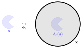
Figure 2: $a$ is a manifold with boundary, independent of $\Sigma$. By specifying an embedding $\phi$, we can think of $a$ as a subset of $\Sigma$ in a gauge invariant way. Throughout this paper, we refer to $\phi_{e}(a)$ as $A$.

The extended Hilbert space in gravity is explicitly given by $\widetilde{\mathcal{H}}_{a}=\mathcal{H}_{a}\otimes L^{2}(ECS)$, where $\mathcal{H}_{a}$ represents the $\text{Diff}(a)$-invariant Hilbert space of bulk operators (including gravitons) localized to $a$, and the $L^{2}(ECS)$ factor represents wave functions over possible embeddings of the region $a$ into the spacetime. Recall that we already cut off $\mathcal{H}_{a}$ to cure UV divergences and make it well defined, essentially by excluding trans-Planckian fluctuations. We will similarly regulate ECS so that we only keep the edge modes necessary to match with the fluctuations below the cut off in the bulk of $a$. This renders the regulated ECS locally compact so that we can use its Haar measure to define an inner product on $L^{2}(ECS)$. We will proceed with this regulator in place and remove it at the end.

Similarly to Yang-Mills theory, ECS acts as a global symmetry group for $\widetilde{\mathcal{H}}_{a}$. We would like to then conclude that $\widetilde{\mathcal{H}}_{a}\sim\oplus_{R}(\widetilde{\mathcal{H}}_{a})_{R}$, where $R$ is an irrep of ECS (regulated to be locally compact). However, mathematically, such a decomposition requires ECS to be “amenable” amenable . This subtlety did not arise in Yang-Mills theory because all compact groups are amenable amenable . Mathematically, amenability means that for all $\epsilon>0$, there is a state $\ket{\alpha}$ such that $|U(g)\ket{\alpha}-\ket{\alpha}|<\epsilon$ for all $U(g)\in\mathcal{U}(L^{2}(ECS))$, the unitary operators on $L^{2}(ECS)$ amenable . This means the trivial representation is “weakly contained” within $L^{2}(ECS)$, i.e., there is a state $\ket{\alpha}$ which ECS leaves approximately invariant. If $G$ is a compact group with Haar measure $d\mu_{g}$, then we could take

$$\ket{\alpha}=\frac{1}{\text{Vol(G)}}\int d\mu_{g}\,U(g)\ket{\Psi}$$

for any state $\ket{\Psi}$, but non-compact groups such as ECS can be more complicated because there is no finite $\text{Vol}(ECS)$ to normalize the group average. We therefore need a way of regulating the group, performing calculations, and taking the limit at the end. As an example of such a limiting definition, there is no normalizable constant function on $L^{2}(\mathbb{R})$, but one can approximate this function arbitrarily well with a gaussian by taking the limit of large variance. A physical way to describe this requirement of amenability is that there exists an approximate vacuum state for the wave functions over embeddings such that $U(g)\ket{\alpha}\approx\ket{\alpha}$ for all $g\in ECS$. Such a vacuum state manifestly satisfies the above condition for amenability. To this end, we regulate the Hilbert space by truncating the dimension of the allowed representations of ECS

$$\widetilde{\mathcal{H}}^{\Lambda}_{a}:=\bigoplus^{\Lambda}_{R}\,\bigoplus_{n=1}^{d_{R}}\left(\widetilde{\mathcal{H}}_{a}\right)_{R,n}\,,$$ (9)

where $\oplus_{R}^{\Lambda}$ means that we sum on irreps $R$ of ECS such that $d_{R}\leq\Lambda$, and $n$ is a multiplicity index, ranging from $1,\cdots,d_{R}$. Note that the latter is not counting the number of states in a particular representation, but the number of times the representation appears in the sum. As explained above in the case of Yang-Mills, this multiplicity actually equals the dimension of the representation $d_{R}$. We refer to this regulated group as $ECS_{\Lambda}$, and take the limit $\Lambda\to\infty$ at the end. This makes the group amenable because $L^{2}(ECS_{\Lambda})$ manifestly decomposes into a direct sum over its irreducible representations.

2.3 Renormalizing the entropy

Given this decomposition (9) of the regulated Hilbert space, as in Yang-Mills theory, any density matrix $\rho_{a}$ which descends from a global state in $\mathcal{H}_{\Sigma}$ can be written in the form

$$\rho_{a}=\sum_{R}^{\Lambda}\sum_{n=1}^{d_{R}}p_{R,n}\,\rho_{R,n}\otimes\frac{1}{d_{R}}\text{Id}_{R,n}\,,$$ (10)

where $\sum_{R}^{\Lambda}$ means that we sum on irreps $R$ of ECS such that $d_{R}\leq\Lambda$, and $n$ is a multiplicity index, ranging from $1,\cdots,d_{R}$. $\rho_{R,n}$ is a state of the purely bulk degrees of freedom, which is a possibly mixed state of fields whose boundary conditions on $\partial a$ transform in a representation $R$ of ECS. Each $\rho_{R,n}$ is a generalization of a “fixed area state” to the full ECS group dong2023holographic , prepared with Dirichlet boundary conditions for the fields at the boundary. The bulk fields transform non-trivially under ECS even though these are diffeomorphisms of the full slice $\Sigma$ because ECS is a global symmetry group for the subregion $a$, as described above. We would like to compute the entropy of this state:

$$S(\rho_{a})=-\tr_{ECS_{\Lambda}}\tr_{a}\rho_{a}\ln\rho_{a}\,.$$ (11)

Because of the superselection over representations, each term in the sum over representations is orthogonal, allowing us to pull the sum out of the log. Additionally, because $S(\rho_{1}\otimes\rho_{2})=S(\rho_{1})+S(\rho_{2})$, we can compute the entropy of each factor seperately and add them together again. All together,

$$S(\rho_{a})=\sum^{\Lambda}_{R}\sum_{n=1}^{d_{R}}-p_{R,n}\ln p_{R,n}+p_{R,n}\ln d_{R}-p_{R,n}\tr_{a}\rho_{R,n}\ln\rho_{R,n}.$$ (12)

The sum on $R,n$ comes from the trace on $ECS_{\Lambda}$ in the representation basis.

The first term in (12) is the Shannon entropy of the distribution over representations. The second is the entropy of the maximally mixed state over the edge modes $\frac{1}{d_{R}}\text{Id}_{R,n}$. The last term is the von Neumann entropy of the bulk fields in the state $\rho_{R,n}$. Here, $\tr_{a}$ denotes the trace over purely bulk degrees of freedom $\mathcal{H}_{a}$, and is well defined for the subregion $a$ because of our bulk regulator. Since the symmetry group has a copy of the gauge group at each point on the corner (the $(\cdots)_{\partial a}$ dependence), the sum over $\ln d_{R}$ will exhibit area scaling (times a factor that diverges as we remove the regulators on ECS). We may therefore wonder if it contributes directly to the area term in the Bekenstein-Hawking entropy. However, this term exhibits area scaling in any gauge theory, so this particular area scaling is not special to gravity. Additionally, all graviton degrees of freedom are encoded within $\rho_{R,n}$, suggesting that this area scaling is a red herring. Indeed, our calculations below will reveal a different origin for the entanglement entropy that we are computing.

As we take $\Lambda\to\infty$, the second sum in (12) diverges for a generic distribution $p_{R,n}$ because of the $\ln d_{R}$ dependence of the entropy, and we must renormalize it. Define

$$\Omega:=\sum^{\Lambda}_{R}\sum_{n=1}^{d_{R}}d_{R}=\sum_{R}^{\Lambda}d_{R}^{2}=\tr_{L^{2}(ECS_{\Lambda})}(\text{Id}_{L^{2}(ECS_{\Lambda})})\,.$$ (13)

One can think of $\Omega$ as the infinite temperature partition function for the microcanonical ensemble over the cutoff embeddings. To absorb the divergence as $\Lambda\to\infty$ (equivalently, $\Omega\to\infty$), we adopt the Susskind-Uglum procedure and simultaneously renormalize $\tr_{a}$ over the bulk states as

$$\tr_{a} \mapsto\Omega^{-1}\tr_{a}\,,$$ (14)

$$\rho_{R,n} \mapsto\Omega\rho_{R,n}\,.$$ (15)

The simultaneous rescaling of $\rho_{R,n}$ is needed to ensure it remains properly normalized under the new trace. Notice that this rescaling is state independent and therefore well defined. In the language of von Neumann algebras, the inverse of our $\Lambda\to\infty$ limit takes the form of a “conditional expectation”. Given two von Neumann algebras $N\subset M$, a conditional expectation is a map $\mathcal{E}:M\to N$ such that for $n_{1},n_{2}\in N$ and $m\in M$, we have that

$$\mathcal{E}(\text{Id}_{M}) =\text{Id}_{N}\,,$$ (16)

$$\mathcal{E}(n_{1}mn_{2}) =n_{1}\mathcal{E}(m)n_{2}\,.$$ (17)

In our case, we take $M=\mathcal{A}_{\Lambda^{\prime}}$ and $N=\mathcal{A}_{\Lambda}$, the von Neumann algebras acting on the regulated Hilbert spaces with cutoffs $\Lambda^{\prime}>\Lambda$. Crucially, the traces in these algebras have been rescaled appropriately by equation (14). The map $\mathcal{E}$ is then given explicitly by

$$\mathcal{E}_{\Lambda^{\prime}\to\Lambda}(\cdot)=\Pi_{\Lambda}\,(\cdot)\,\Pi_{\Lambda}$$ (18)

where $\Pi_{\Lambda}$ is the projector onto the $\widetilde{\mathcal{H}}^{\Lambda}_{a}$ subspace of $\widetilde{\mathcal{H}}^{\Lambda^{\prime}}_{a}$. One can see explicitly that this map satisfies the properties of a conditional expectation, which has recently been connected to the Susskind-Uglum procedure gesteau2023large .

Applying this rescaling to the entropy formula (12), and noting the $\ln\rho_{R,n}$ dependence, we can rearrange the terms as

$$S(\rho_{a}) =\sum^{\Lambda}_{R}\sum_{n=1}^{d_{R}}-p_{R,n}\ln p_{R,n}+p_{R,n}\ln d_{R}-p_{R,n}\ln\Omega-p_{R,n}\tr_{a}\rho_{R,n}\ln\rho_{R,n}$$ (19)

$$=\sum^{\Lambda}_{R}\sum_{n=1}^{d_{R}}-p_{R,n}\ln p_{R,n}+p_{R,n}\ln\left(\frac{d_{R}}{\Omega}\right)-p_{R,n}\tr_{a}\rho_{R,n}\ln\rho_{R,n}$$ (20)

$$=-S_{rel}\left(p_{R,n}\left|\frac{d_{R}}{\Omega}\right)\right.-\sum^{\Lambda}_{R}\sum_{n=1}^{d_{R}}p_{R,n}\tr_{a}\rho_{R,n}\ln\rho_{R,n}$$ (21)

where $S_{rel}$ is the relative entropy between the indicated distributions.

How does the value of the entropy depend on the specific renormalization scheme we adopt here? If we instead picked a scheme where we rescaled the trace over bulk states by $e^{S_{0}}\Omega$, we would simply shift the entropy by a state independent constant $S_{0}$, implying a single ambiguity. This is characteristic of states belonging to type II von Neumann algebras, consistent with recent investigations of quantum gravity in subregions in Leutheusser:2022bgi ; Witten_2022 ; Chandrasekaran_2023 ; Jensen:2023yxy ; kudlerflam2023generalized .

We assumed that the global state $\ket{\Psi}$ was well described not just by a gauge invariant state, but by a semi-classical state. Intuitively, a semi-classical geometry should be represented by a coherent state over the embeddings $\phi_{g}$. In other words, we expect the wave function in $L^{2}(ECS)$ to be Gaussian. But we also expect this wave function to be highly peaked around a particular embedding: semi-classically, the region $a$ has a definite coordinate location within the spacetime. This implies a large uncertainty in the area of the region. To see this, note that fixing the boost angle of $a$, i.e., the choice of time slice which is part of the data of the embdedding, leads to a large variance in the area, as these are conjugate variables. The area is determined by the boundary value of fields such as the gravitons, which are a function of the state, explaining how a region could have a definite embedding but indefinite area. In the end, when we take the saddlepoint in $G_{N}\to 0$ limit, the region $a$ will have both a definite embedding and area as the uncertainty principle relating area and boost angle is $\sim G_{N}$ and so becomes trivial in the semiclassical limit.

As discussed above, each $\rho_{R,n}$ is prepared with Dirichlet boundary conditions for the bulk fields. Thus, by the Heisenberg uncertainty principle, a definite embedding demands a flat distribution over representations. The microcanonical flatness of $p_{R,n}$ simply indicates that the embedding is semiclassically well localized. The information about the particular embedding is encoding in the phases appearing in the density matrices of each representation $\rho_{R,n}$. Thus, the flat distribution over $R$ corresponds to taking $\rho_{a}$ to have Neumann boundary conditions for bulk fields at the corner.

The flatness of $p_{R,n}$ for semi-classical states has appeared before in the literature. For example, we can view this condition as a rephrasing of Jacobson’s entanglement equilibrium hypothesis, which posits that the semi-classical vacuum is the maximal entropy state Jacobson_2016 . For sufficiently symmetric regions $a$, this condition is sufficent to recover the semi-classical Einstein equations. It is also consistent with the “slowly-varying” semi-classical assumptions on the observer wavefunctions in Leutheusser:2022bgi ; Witten_2022 ; Chandrasekaran_2023 ; Jensen:2023yxy ; kudlerflam2023generalized , suggesting their observer should be thought of as a subset of the edge modes. This identification also makes intuitive sense, since the observer in Leutheusser:2022bgi ; Witten_2022 ; Chandrasekaran_2023 ; Jensen:2023yxy ; kudlerflam2023generalized is an abstract model of a clock, and embedding the region $a$ into partial time slices related by a boost keeping $\partial a$ fixed within the spacetime is one way to measure time within $a$. In fact, in the language of algebras, the mathematical description of a gravitating observer and the edge modes takes a remarkably similar form klinger2023crossed .

These arguments all suggest that we should take Neumann boundary conditions for the bulk fields within $a$. At the level of the representations, this implies we can at least approximately replace $p_{R,n}\to\frac{d_{R}}{\Omega}$ for large enough $\Omega$. This substitution makes the relative entropy in equation (21) vanish. Finally, we can substitute this form for $p_{R,n}$ in the average over bulk entropies. To recap, we have argued that the entropy for an arbitrary semi-classical state $\rho_{a}$ takes the form

$$S(\rho_{a}) =\frac{1}{\Omega}\sum_{R}^{\Lambda}\sum_{n=1}^{d_{R}}d_{R}\left[-\tr_{a}\rho_{R,n}\ln\rho_{R,n}\right]$$ (22)

$$=\frac{1}{\Omega}\sum_{R}^{\Lambda}\sum_{n=1}^{d_{R}}\sum_{m=1}^{d_{R}}\left[-\tr_{a}\rho_{R,n}\ln\rho_{R,n}\right]\,.$$ (23)

We replaced the factor of $d_{R}$ with a sum over an auxiliary variable $m$ for later convenience. The fact that $\rho_{R,n}$ is independent of $m$, i.e., it is microcanonically flat within each representation, is expected from AdS/CFT Akers_2019 ; Dong_2019 ; Harlow_2017 and plays a crucial role in the quantum error correction underlying complementary recovery. In our case, flatness can be traced back to the factorization $\rho_{R,n}\otimes\text{Id}_{R,n}$ within each superselection sector, which in turn was a consequence of diffeomorphism invariance in the global state. This suggests it is the bulk diffeomorphism invariance which leads to holographic recovery.

We will now explain why the sum in equation (23) can be regarded as a trace over $L^{2}(ECS_{\Lambda})$. First, as explained in Sec. 2.1, for compact groups $G$, the regular representation $L^{2}(G)$ has a decomposition (4). In particular, we can decompose the trace on $L^{2}(G)$ as

$$\tr_{G}(\cdot)=\sum_{g\in G}\bra{g}\cdot\ket{g}=\sum_{R}^{\Lambda}\sum_{n=1}^{d_{R}}\sum_{m=1}^{d_{R}}\bra{R,n,m}\cdot\ket{R,n,m}$$ (24)

where $m$ is a label on the microstates within each representation $R,n$. This expression for the trace also holds for the regulated $ECS_{\Lambda}$ by the definition of our regulator. The first equality expresses the trace as a sum over equivalence classes of embeddings $\phi_{g}$ of $a$ modulo the diffeomorphisms $\text{Diff}(a)$, and the second equality expresses the trace in the Fourier basis, i.e., the sum on representations of $ECS_{\Lambda}$. We now recognize (23) as a regulated definition of the trace over $ECS_{\Lambda}$ in equation (11). Writing this trace in the basis of embeddings as in the first equation in (24) we arrive at our final regulated formula

$$S(\rho_{a}) =\frac{\tr_{ECS_{\Lambda}}}{\Omega}\left[-\tr_{a}\rho[\phi_{g}]\ln\rho[\phi_{g}]\right]$$ (25)

Here, $\rho[\phi_{g}]$ is a bulk state with boundary conditions set by a definite coordinate embedding $\phi_{g}$, as opposed to the definite charge of $\rho_{R,n}$. In the limit $\Omega\to\infty$, the trace $\tr_{ECS_{\Lambda}}$ becomes a path integral, as does $\tr_{a}$. Because $\Omega=\tr_{ECS_{\Lambda}}\text{Id}_{ECS_{\Lambda}}$, this regularization procedure has also recovered precisely the correct normalization for the path integral. So we can now remove the cutoff on the edge modes and send $\Omega\to\infty$, to arrive at a path integral for the the entropy:

$$S(\rho_{a})=-\int_{ECS}D\phi_{g}\,D(\phi_{g}^{*}\chi)\,\rho_{a}[\phi_{g},\phi^{*}_{g}\chi]\ln\rho_{a}[\phi_{g},\phi^{*}_{g}\chi]$$ (26)

In this path integral, we integrate over the gauge fixed definitions of the embeddings $\phi_{g}$. $\chi$ is a bulk field defined on $\phi_{g}(a)$, i.e., the embedding of $a$ into $\Sigma$, while $\phi^{*}_{g}$ is the pullback from $\phi_{g}(a)\to a$. In other words, $\phi^{*}_{g}\chi$ are the matter fields defined on the model region $a$. These are the fields prepared by $\tr_{a}$ because this trace was defined on the Hilbert space $\mathcal{H}_{a}$ of the model region.

It is more convenient to instead integrate over the fields $\chi$ instead, i.e., fields defined on the target space $\phi_{g}(a)$. Additionally, we wish to sum over all embeddings $\phi$, not simply the gauge fixed equivalence classes. In doing so, we must divide by a volume factor $|\text{Diff}(\phi,\chi)|$ to remove the overcounting. $|\text{Diff}(\phi,\chi)|$ divides out all diffeomorphisms with support on $\phi(a)$, because this is the domain of the fields $\chi$. Making these substitutions, we find that the entropy of a region $a$ is given by

$$S(\rho_{a})=-\int\frac{D\phi D\chi}{|\text{Diff}(\phi,\chi)|}\,\rho_{a}[\phi,\chi]\ln\rho_{a}[\phi,\chi]\,.$$ (27)

3 Computing the entropy

3.1 A path integral proposal

Above, we constructed a formula for the entropy of a bulk region $a$. We will now explicitly evaluate this entropy via the replica trick, which proceeds as follows. For an arbitrary quantum state $\rho$, we first define the Renyi entropy as

$$S_{n}(\rho)=\frac{1}{1-n}\ln\tr\rho^{n}\,.$$ (28)

The von Neumann entropy is given by the limit

$$S(\rho)=\lim_{n\to 1}S_{n}(\rho)=-\partial_{n}\tr(\rho^{n})|_{n=1}\,.$$ (29)

Thus, to calculate the entropy we must compute the trace of powers of $\rho_{a}[\phi,\chi]$. We will use the gravitational path integral defined below to perform this computation.

To recap, $\phi:a\hookrightarrow\Sigma$ is an embedding, as above. By letting $\phi$ fluctuate, the region $\phi(a)$ itself moves around within $\Sigma$, while $a$ is independent of $\phi$. To see that $\phi$ can really move the region within the spacetime, consider two distinct embeddings $\phi_{1}$ and $\phi_{2}$. Depending on their images, it is possible that $\phi_{1}(a)\cap\phi_{2}(a)=\emptyset$. This would not be possible if $\phi_{1,2}$ did not move the region $a$ within the slice $\Sigma$. This is an active view of the role of the embeddings. Alternatively, we can view the embedding as keeping $a$ fixed, while changing the coordinate definition of $\partial a$. Because $\Sigma$ has a fixed background metric, these coordinate transformations move the points within $\Sigma$ into and out of the region. This is a passive view of the role of the embeddings $\phi_{1,2}$.

We now wish to define the path integral computing the (unnormalized) trace of $\rho_{a}$, i.e., the partition sum ${\cal Z}(a)$, for a subregion $\phi(a)$. Let $\chi$ be bulk fields, including perturbative gravitons, defined on $\phi(a)$. It is important that the dynamical fields are $(\chi,\phi)$, not $(\phi^{*}\chi,\phi)$, where $\phi^{*}$ is the pullback, i.e., $\chi$ is defined in the target space $\phi(a)$ and not the model region $a$. Of course, these two sets of variables are equivalent, so one could work with the other choice instead Speranza_2018 , but our convention turns out to be more natural one for future computations. By the same reasoning as in the previous section, we impose Neumann boundary conditions at the corner for the bulk fields $\chi$. We then propose that the partition sum for an arbitrary bulk subregion $\phi(a)\subset\Sigma$ can be computed by the following gravitational path integral that is consistent with the diffeomorphism constraints:

$$\tr(\rho_{a}) =\mathcal{Z}(a)=\int\frac{D\phi D\chi}{|\text{Diff}(\phi,\chi)|}e^{-S[\phi,\chi]}$$ (30)

$$S[\phi,\chi] =\int_{D[\phi(a)]}\mathcal{L}[\chi]=\int_{D[a]}\phi^{*}\mathcal{L}[\chi]$$ (31)

Here, by $D[\phi(a)]$ we mean the domain of dependence generated by the partial Cauchy slice $\phi(a)$, and $D[a]$ is the corresponding model causal development. $\mathcal{L}[\chi]$ is the Lagrangian for the effective field theory defined on $D[\phi(a)]$, in our case the Einstein-Hilbert Lagrangian plus matter terms, but more generally we could take any covariant (i.e., diffeomorpism invariant) Lagrangian. $\phi^{*}$ is the pullback of the Lagrangian to $a$. From the perspective of $a$, the pullback is the only way the edge modes $\phi$ enter into the action. From the perspective of the target space, $\phi$ only enters by determining the domain of dependence $D[\phi(a)]$ over which we should evaluate the action. $|\text{Diff}(\phi,\chi)|$ is the volume of the group of diffeomorphisms with compact support on $\phi(a)$. This is the gauge symmetry for $\phi(a)$. One can think of $a$ as describing a gauge invariant notion of the region and $\phi$ as characterizing the fluctuations of this region.

Importantly, $D\phi$ is the flat measure on embeddings. This followed from the fact that the measure $\frac{1}{\Omega}$ in our regulated sum over representations (23) and (25) was independent of ECS. This measure (and therefore $\mathcal{Z}(a)$) was specified by demanding that the background state be semiclassical and gauge-invariant, which meant that it was micronanonically flat in the corner symmetry representation basis for the embedding of $a$ into $\Sigma$. Equivalently, $\mathcal{Z}(a)$ can be thought of as simply being $\mathcal{Z}(\Sigma)$ with the fields on $a^{\prime}$ traced out. The fact that the measure we arrived at is essentially unique suggests that the particular regulator scheme we adopted above does not affect the final result. Recall from equations (14) and (15) that the regulator on the bulk fields also depends on the edge mode regulator in a way that cancels the divergences in the edge mode sector. This suggests that our result is also independent of the details of our bulk regulator. This novel proposal for the path integral of a finite region is our main technical tool.

Returning to the Reyni entropy (29), we need to compute $\tr(\rho_{a}^{n})$. Following our path integral expression in (30) for $\tr(\rho_{a})$, we can prepare $\tr(\rho_{a}^{n})$ by computing $\mathcal{Z}(a^{n})/\mathcal{Z}(a)^{n}$ on an n-fold replica of the model region $a$ (equivalently, $\phi(a)$). In other words, we have to compute

$$S(\rho_{a})=-\partial_{n}\left(\frac{\mathcal{Z}(a^{n})}{\mathcal{Z}(a)^{n}}\right)_{n=1}$$ (32)

Explicitly in terms of the path integral,

$$S(\rho_{a}) =-\partial_{n}\left[\int D\phi_{(n)}\int_{a^{n}}\frac{D\chi}{|\text{Diff}(\phi_{(n)},\chi)|}\frac{e^{-S[\phi_{(n)},\chi]}}{\mathcal{Z}(a)^{n}}\right]_{n=1}$$ (33)

The subscript $(n)$ indicates that this is a path integral over embeddings of the $n-$fold replica $a^{n}$, not simply a single copy of $a$. One can think of $\phi_{(n)}$ as a vector of embeddings for the copies of $a$ to be glued together. The boundary conditions of the fields are the same for each copy, but generically, the specific details of $\phi_{(n)}$ away from each copy of $\partial a$ can differ in detail.

We will be interested in the value of the entropy in the semiclassical limit $G_{N}\to 0$, so we can take a saddlepoint approximation for the $\chi$ integral in both the numerator and the denominator. However, because the normalizing volume factor $|\text{Diff}(\phi,\chi)|$ depends on $\chi$, we must include variations of this factor in the saddle point equation. We will outline this procedure explicitly in the next section, and find that the physical configurations of the embeddings, which we denote by $\varphi$, only include fluctuations which are strictly larger than (or equal to) the original region $A$. Letting $I_{n}[\varphi_{(n)}]$ denote the on-shell effective action of the $n-$replicated manifold for a fixed $\varphi_{(n)}$, this gives

$$S(\rho_{a}) =-\partial_{n}\left[\frac{\int_{a^{n}}D\varphi_{(n)}e^{-I_{n}[\varphi_{(n)}]}\,}{\left(\int_{a}D\varphi_{(1)}e^{-I_{1}[\varphi_{(1)}]}\right)^{n}}\right]_{n=1}\,.$$ (34)

We do not impose any smoothness requirement on the replicated (partial) saddles $\varphi_{(n)}(a^{n})$ or $\varphi_{(1)}(a)$ at this time; at the present stage, the embeddings $\varphi$ can be off-shell and act as a source for possible singularities.

3.2 Why outward deformations

To characterize the classes of physical embeddings $\varphi$, we expand the partition sum (30) in the limit of small fluctuations around the original embedding, which we refer to as $A$ as above. We focus on the $n=1$ case for concreteness, as the higher $n$ case is conceptually the same. To clarify our notation, by $\phi$, we mean all embeddings of $a\hookrightarrow\Sigma$ irrespective of their relationship under small diffeomorphisms, i.e., they can be related by gauge transformations. By $\phi_{g}$, we mean the equivalence classes of $\phi$ under small diffeomorphisms, which are labeled by an element of ECS as described in Sec. 2. Finally, by $\varphi$, we mean the embeddings which survive after accounting for the gauge fixing determinant in the $\chi$ saddle point. We now argue that $\varphi$ only contains fluctuations such that $\varphi(a)$ strictly contains $A$. As we will see, it is the diffeomorphism invariance of the target space which breaks the symmetry between inward and outward fluctuations. This is intuitively true because we specified the problem by saying that we have complete information about the state within $a$, and an inward fluctuation would seem to “erase” part of this information.

In the partition function (30), we are integrating over $\phi$ and $\chi$, which are bulk fields defined on the target space $\phi(a)$. This means that the divisor $|\text{Diff}(\phi,\chi)|$ is the volume of the group of diffeomorphisms with support on $\phi(a)$. To simplify our analysis, we take the limit of small fluctuations in $\phi$ around $\phi_{e}$, the embedding defining the region $A$. In this limit, there are two distinct types of diffeomorphisms: ones which do move the boundary $\partial A$, and ones which do not. Because we take the limit of small fluctuations, the volume divisor factorizes into

$$|\text{Diff}(\phi,\chi)|\approx|\text{Diff}(\phi_{e},\chi)|\cdot|\text{Diff}(\phi,\chi_{e})|$$ (35)

where $|\text{Diff}(\phi_{e},\chi)|$ is the volume of diffeomorphisms which do not move the corner, but do move the fields within $A$, and $|\text{Diff}(\phi,\chi_{e})|$ is the volume of diffeomorphisms which do move the corner but leave the bulk fields unchanged. The factorization follows because in the strict $G_{N}=0$ limit the diffeomorphisms are irrelevant and are therefore uncoupled. So this factorization holds approximately in the weak coupling limit, and the path integral can be written as

$$\mathcal{Z}(a)=\int\frac{D\chi D\phi}{|\text{Diff}(\phi_{e},\chi)|\cdot|\text{Diff}(\phi,\chi_{e})|}e^{-S[\phi,\chi]}\,.$$ (36)

Additionally, in this limit, we can split the measure for the embeddings into the gauge orbits and the gauge degrees of freedom in the usual way via field redefinitions. Because of the diffeomorphism invariance of the action, the integral over small fluctuations of the boundary gives a volume factor, as well as a determinant from the change of variables. This volume factor is precisely $|\text{Diff}(\phi,\chi_{e})|$ because we are in the weak coupling limit, so that the effect of moving $\chi$ at the same time as $\phi$ is a higher order effect. This is analogous to non-abelian Yang-Mills. Explicitly, the measure splits as

$$D\phi=D\phi_{g}\,|\text{Diff}(\phi,\chi_{e})|\det(\cdots).$$ (37)

where $\phi_{g}$ are the gauge orbits of the embeddings labeled by elements of ECS, $|\text{Diff}(\phi,\chi_{e})|$ is the volume factor discussed above, and $\det(\cdots)$ is the gauge fixing determinant. Plugging this into (36),

$$\mathcal{Z}(a) \approx\int\frac{D\chi D\phi_{g}}{|\text{Diff}(\phi_{e},\chi)|}\det(\cdots)e^{-S[\phi,\chi]}$$ (38)

$$=\int\frac{D\chi D\phi_{g}D[\text{ghosts}]}{|\text{Diff}(\phi_{e},\chi)|}e^{-S[\phi,\chi]-S_{ghosts}}$$ (39)

where we have used the ghost representation of the gauge fixing determinant in the second line.

Now consider an analogy. In non-Abelian Yang-Mills theory, the role of the ghosts is to eliminate the unphysical timelike and longitudinal degrees of freedom from the path integral. These unphysical polarizations are a remnant of the residual gauge symmetry left over after gauge fixing. If one could explicitly separate the gauge orbits into those with physical (transverse) and unphysical polarizations, then the ghost action would exactly cancel the unphysical polarizations and leave an integral over just the physical degrees of freedom. Thus, by identifying gauge orbits which are related by the residual gauge symmetry, we can remove the unphysical polarizations and can eliminate the ghosts. We will now do this for our gravitational path integral.

We have expanded the path integral around $A=\phi_{e}(a)$ as above. Here, the ghosts will explicitly cancel particular configurations $\phi_{g}$ from the path integral, and will leave behind only the physical embeddings $\varphi$. We now argue that these physical embeddings are strictly larger than $\phi_{e}$, the original embedding we expanded around.

Let $\delta_{g}$ be a diffeormorphism with support on the corner of the original embedding $\partial A$, such that $\phi_{g}(a):=\delta_{g}\cdot\phi_{e}(a)$, and furthermore assume that $\phi_{g}(a)\subset A$, i.e., $\delta_{g}$ is an inward deformation. Because $\phi_{g}(a)$ is a subset of the original embedding, there exists a diffeomorphism with support on $A$ which makes $\phi_{g}(a)$ arbitrarily close to $A$. This means that they are gauge equivalent under the residual gauge symmetry $\text{Diff}(\phi_{e},\chi)$, which is the relevant group of diffeomorphisms to consider because the remaining divisor term is precisely $|\text{Diff}(\phi_{e},\chi)|$. Therefore, the ghost degrees of freedom will explicitly cancel this contribution, and we can discard it from the path integral. On the other hand, consider $\phi_{g^{-1}}:=\delta_{g}^{-1}\cdot\phi_{e}(a)\supset A$, i.e., an outward deformation. Then, there is no diffeomorphism with support on $A$ which can equate them: they are in different equivalence classes under the residual gauge symmetry. Therefore, the ghost degrees of freedom will not cancel this contribution, and we must include it in the path integral. See Fig. 3. Thus, to leading order in perturbation theory, the only remaining embeddings to sum over strictly satisfy $\varphi(a)\supset A$, namely, embeddings $\varphi:a\hookrightarrow\Sigma$ that strictly include the original region $A$ to leading order in $G_{N}$. In Sec. 3.4, we will argue that this strict containment persists to all orders in perturbation theory.

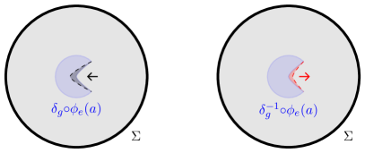
Figure 3: Two examples of diffeomorphisms which can change the embedding map. Left: The deformation moves the new region (blue) strictly inside the original region $A$ (blue and black). The residual gauge symmetry is diffeomorphisms with support on $A$ (blue and black): such a diffeomorphism can push the boundary back to the original configuration. Right: The deformation moves the new region (blue and red) strictly outside the original one $A$ (blue). The residual gauge symmetry is diffeomorphisms with support on $A$ (blue): such a diffeomorphism can never pull the boundary back to the original configuration.

3.3 Imposing the saddlepoint equation

Returning to the entropy computation (34), because the effective action $I_{n}$ is $\mathcal{O}(G_{N}^{-1})$, we must also take a saddlepoint limit of the remaining path integral over physical embeddings $\varphi$ for consistency. Letting $E_{(n)}$ be the embedding which solves this saddlepoint equation, we can approximate the entropy as

$$S(\rho_{a}) =-\partial_{n}\left[e^{-I_{n}[E_{(n)}]+nI_{1}[E]}\right]_{n=1}$$ (40)

where we have condensed the notation a bit so $E:=E_{(1)}$. For simplicity, we assume that $E(a)$ is unique and homotopic to $A$; we consider the more general case at the end of this section. Note that $E(a)\supset A$ by the argument in the previous section. We now show this implies that $\partial E(a)$ must be extremal at points where it does not coincide with the original corner, i.e., $\partial A\neq\partial E(a)$, and is unconstrained wherever $\partial A=\partial E(a)$.

The saddlepoint equation is equivalent to requiring $E_{(n)}(a^{n})$ be on-shell. As we showed in Sec. 2, when gluing two spacetime subregions together, one must use the entangling product to ensure compatibility between the Hamiltonian charges generating diffeomorphisms in the glued spacetime. This is sufficient for the glued spacetime to be on-shell, because it will satisfy the diffeomorphism constraints. Usually, this compatibility of charges is between $a$ and $a^{\prime}$, as is explained in Sec. 2.1 and Sec. 2.2. Given any embedding for $a$, one can choose an embedding for $a^{\prime}$ to ensure the glued spacetime is smooth. But for the replicated space, the constraint must instead be enforced between $n$ copies of $a$ itself. Recall that we viewed the corner symmetry ECS in two different ways: one is as the group of diffeomorphisms with support on $\partial a$, and the other was as parameterizing the space of embeddings of $a\hookrightarrow\Sigma$. Taking the saddle $\phi=E$ is therefore equivalent to picking a single vector field $\xi$ which generates the diffeomorphism from $A$ to $E(a)$, and imposing the constraint from this particular diffeomorpism. We now compute this Hamiltonian charge, and will see that its vanishing, which imposes the constraint, implies the extremality condition we outlined above.

A simple way to explain the expression for this Hamiltonian charge is by using the Hamilton-Jacobi equation, or Schwinger’s principle in the quantum case. The Hamilton-Jacobi equation says that if one varies the on-shell action $I$ with respect to a generalized coordinate $x$, then $\partialderivative{I}{x}=p$, where $p$ is the generalized momentum generating a translation in $x$. The application of this principle to our setting can be more rigorously justified using covariant phase space techniques Wald_1993 ; Iyer_1994 ; Iyer_1995 , and relies on the fact we are using the extended phase space of Ciambelli and Leigh Ciambelli_2021 ; Ciambelli_2022 ; klinger2023crossed ; klinger2023extended . In our setting, the “momentum” is the Hamiltonian charge $H_{\xi}$ which generates the diffeomorphism parameterized by $\xi$. The charge $H_{\xi}$ contains linear combinations of the equations of motion, so its vanishing also implies that $E_{(n)}(a^{n})$ is on-shell.

One example of a saddle for the replicated manifold is given by $(E(a))^{n}$, the $n=1$ saddle glued cyclically $n$ times. We will assume that this replica symmetric saddle is dominant. The relevant total charge which must vanish is thus

$$\sum_{i}H^{a_{i}}_{\xi}=nH_{\xi}=0\,.$$ (41)

This implies that $H_{\xi}=0$ is the constraint for $E(a)$ to be on-shell. Explicitly, let $x_{\xi}$ be a coordinate of the flow on $\Sigma$ generated by $\xi$. The Hamilton-Jacobi equation (or Schwinger’s principle in the quantum case) says that the charge is given by

$$H_{\xi}=\frac{1}{n}\partialderivative{I_{n}}{x_{\xi}}=\int_{\partial E(a)}\xi\Theta=0$$ (42)

where $\Theta$ is a local functional defined on the corner $\partial E(a)$ called the generalized expansion Wald_1993 ; DLR_2016 . For example, we will see below that when the matter contributions to the effective action can be neglected, $\Theta=K$, where $K$ is the trace of the extrinsic curvature freidel2023corner . More specifically, if $\xi=\partial_{r}$, where $r$ is a radially outward coordinate, then $\xi\Theta=K^{r}$.

But crucially, $H_{\xi}$ is linear in $\xi$, and so the integrand vanishes wherever $\xi=0$ along $\partial E(a)$. This implies that if $\xi=0$ at a point $p$, then $\Theta$ can take any value at $p$ and we will still satisfy the constraint $H_{\xi}=0$. By definition of $\xi$, at a point $p$, $\xi|_{p}=0$ if and only if $\partial E(a)|_{p}=\partial A|_{p}$. So, by locally varying each point on the corner $\partial E(a)$, we can see that the saddle point equation requires $\Theta=0$ when $\partial E(a)\neq\partial A$, and is otherwise unconstrained. This is essentially the same as the result of Lewkowycz-Maldacena Lewkowycz_2013 when they derived the Ryu-Takayanagi formula Ryu_2006 , except we have the possibility of $\xi=0$ because $a$ can be a finite region. Another way to phrase this result is that the fields at points where $\partial A=\partial E(a)$ are on-shell because they are constant on the contour of steepest descent and therefore extremize the action on this contour, while the fields at points where $\partial A\neq\partial E(a)$ are on-shell because of the extremality condition of the generalized expansion.

We can also justify as follows that $E(a)$ can be finitely far from $A$. Recall that in Sec. 3.2, we argued that to leading order in perturbation theory around $A$, the physical embeddings $\varphi(a)$ in the path integral strictly contain $A$, i.e., only contain outward deformations. To find the saddlepoint $E(a)$, we can use gradient descent from $A$ to flow towards this solution. By repeating the arguments of Sec. 3.2 for the perturbatively flowed solution, we can see that the outward-only property of the physical embeddings persists to all orders in perturbation theory. This gives an intuitive picture of the intermediate homotopy surfaces between $A$ and $E(a)$ as carrying the information from $\partial A$ to $\partial E(a)$ and vice versa. Because this gradient descent argument comes from a path integral, we can remove the uniqueness assumption on $E(a)$ by taking the minimum over all possible saddles homotopic to $a$.

In this calculation, we assumed that $A$ was homotopic to $E(a)$ for simplicity of discussion, which amounts to assuming that $A$ and $E(a)$ have the same topology. A possible argument extending our results to general topologies for $E(a)$ is as follows. The condition that $A$ and $E(a)$ are homotopic can be traced back to the assumption that $\phi$ was an embedding. Embeddings are globally constrained to be one-to-one, and such global constraints on field configurations are unnatural without the presence of symmetries to impose them. A more natural specification for the maps $\phi:a\hookrightarrow\Sigma$ is to demand that $\phi$ is only locally an embedding, i.e., it is an immersion. This relaxation from embeddings to immersions amounts to summing over all topologies for $\phi(a)$. These non-perturbatively different sectors were not apparent from the discussion about edge modes because edge modes were defined perturbatively around the region $a$. Because we defined the bulk fields $\chi$ in terms of the target space $\phi(a)$, we can sum over the topologies of $\phi(a)$ in equation (30) without ambiguity. The rest of analysis of in Sec. 3 then proceeds the same way, modulo replacing $A$ with topologically different configurations $\phi_{e,\gamma}(a)$ to expand around, where $\gamma$ is an index labeling the topological details of $\phi_{e,\gamma}(a)$. The fact that we chose $A$ to be homeomorphic to $a$ instead of $\phi_{e,\gamma}(a)$ is what distinguishes the original region from these topologically distinct configurations. Furthermore, considering the transitions from one topological sector to another shows that it will still be true that $\phi_{g,\gamma}\supset\phi_{e}$, independent of the topology of $\phi_{g,\gamma}(a)$. Thus, in principle we can remove the restriction that $a$ was homotopic to $E(a)$ and merely require that $a$ is homologous to $E(a)$, as this will remain true regardless of the topology of $\partial E(a)$.

3.4 The final entropy formula

We can now finish the computation of the entropy. Let $I_{n}=n\widetilde{I}_{n}$, where $\widetilde{I}_{n}$ is the on shell action for the $\mathbb{Z}_{n}$ orbifolded version of the replica-symmetric spacetime $(E(a))^{n}$. This orbifold is diffeomorphic to $E(a)$, modulo a conical singularity along $\partial E(a)$, which is a fixed point of the $\mathbb{Z}_{n}$ replica symmetry. In terms of $\widetilde{I}_{n}$, the entropy (40) is

$$S(\rho_{a}) =\partial_{n}\left[I_{n}[E_{(n)}]-nI_{1}[E]\right]_{n=1}$$ (43)

$$=n\partial_{n}\left[\widetilde{I}_{n}[E]-I_{1}[E]\right]_{n=1}$$ (44)

To evaluate the on shell action, we can perform computations similar to the ones done by Lewkowycz and Maldacena in Lewkowycz_2013 . The bulk contributions cancel from the $I_{1}[E]$ normalization, while the remaining boundary terms in $\widetilde{I}_{n}[E]$ reduce to the Wald entropy Wald_1993 evaluated on $\partial E(a)$ to leading order in $G_{N}$ via a conical singularity at $\partial E(a)$ as in Lewkowycz_2013 . Explicitly, if we neglect the matter fields, the entropy evaluates to

$$S(\rho_{a})=\left.\frac{1}{8G_{N}}\partial_{n}\int_{\partial E(a)}\left(\nabla^{\mu}g_{\mu r}-g^{\mu\nu}\nabla_{r}g_{\mu\nu}\right)\right|_{n=1}=\frac{A(\partial E(a))}{4G_{N}}$$ (45)

where $r$ is a local coordinate radially outward to $\partial E(a)$, which is defined by $r=0$ in these coordinates.

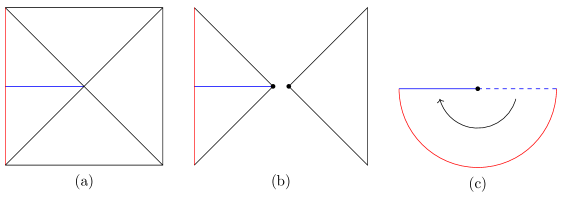
Figure 4: (a) Penrose diagram of AdS₂ showing the domains of dependence of a half-infinite interval and its complement. Herer, the blue interval is $A$. (b) The edge modes allow us to split the left and right wedges into two disconnected spacetimes. Here, the blue interval is $a$. They are disconnected because the extended Hilbert space factorizes, and thus the two subregions are unentangled. To regain the original AdS₂ spacetime, we must glue these wedges at the corner (the black dot) using the entangling product. (c) Euclidean state preparation of $a$ and its edge modes. The solid blue line is the “ket” and the dashed blue line is the “bra”. The direction of the Euclidean time evolution is shown with the arrow. This is not a Cauchy slice for AdS₂: it is a density matrix for the left Rindler wedge.

As a specific example of this calculation, let us consider intervals in AdS₂ in the vacuum state. For the sake of comparison, we first illustrate the more familiar case when $a$ is a half-infinite interval which is partially anchored to the asymptotic boundary (Fig. 4a). The mixed state $\rho_{a}$ can be prepared by Euclidean time evolution as follows. The introduction of edge modes embeds the Hilbert space associated to (Fig. 4a) into a larger one which explicitly factorizes. By considering the universal behavior of entanglement in quantum field theory, this factorization implies each factor lives on a disconnected Cauchy slice, along with edge modes which live at the corners shown as black dots (Fig. 4b). To recover the original Hilbert space, we must identify these edge modes using the entangling product, which glues these two regions along their respective corners. The “future and past” wedges of the original AdS₂ spacetime are then determined by solving the diffeomorphism constraint associated with time evolution. These constraints hold on the global spacetime by construction of the entangling product.

Now consider the Lorentzian construction of the density matrix $\rho_{a}$. We can construct the density matrix by time evolving the boundary conditions at past and future and past causal horizons in the left wedge to the partial $t=0$ slice (with the trivial boundary condition at infinity). This a boost-like evolution, i.e., a modular time evolution of the state which keeps the corner fixed. Alternatively, we can start with the $t=0$ slice and time evolve to the future horizon. By time reflection symmetry, the boundary conditions on the future and past causal horizons in the left wedge in Fig. 4b are the same, so we can analytically continue the contour to the past horizon. We then continue evolving forward in time until reaching the $t=0$ slice. The first approach considers the density matrix as a function of the boundary conditions, and the second approach treats the boundary conditions as a function of the density matrix. But both approaches are equivalent.

By analytically continuing the second procedure we arrive at a convenient description of the Euclidean state preparation for $a$. We note first that Lorentzian (modular) time evolution in the domain of dependence $D[a]$ is most closely analogous to Rindler time because of the boost-like nature of modular flow near $\partial a$. Lorentzian boosts analytically continue to Euclidean rotations, which indicates that Euclidean time evolution will geometrically look like a copy of $a$ “sweeping out” a half disk in an angular direction due to the connection between Euclidean time translations and rotations. The initial copy of $a$ is the “bra”, and the final copy of $a$ is the “ket”. The corner $\partial a$ serves as the origin for this Euclidean rotation because it is a fixed point under Lorentzian (modular) time evolution, so it will continue to be a fixed point after analytic continuation. The endpoint of $a$ which is attached to the asymptotic boundary, however, is not fixed under Lorentzian time evolution, and the Euclidean manifestation of this is the non-trivial boundary of the half-disk (Fig. 4c).

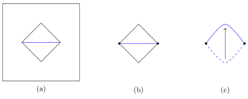
Figure 5: (a) Penrose diagram of AdS₂ showing the domains of dependence of a finite interval and its complement. Here, the blue interval is $A$. (b) The edge modes allow us to split the interval and its complement into disconnected spacetimes (we only show the finite region here). Here, the blue interval is $a$. They are disconnected because the extended Hilbert space factorizes, and thus the two subregions are unentangled. To regain the original AdS₂ spacetime, we must glue $a$ and its complement at their corners (the black dots) using the entangling product. (c) Euclidean state preparation of the density matrix of $a$ and its edge modes. The solid blue line is the “ket” and the dashed blue line is the “bra”. The direction of the Euclidean time evolution is shown with the arrow. One might worry whether this evolution is well-defined, in other words, whether is a sensible Hamiltonian on just this wedge and its edge modes. The evolution is in fact defined, because the Hamiltonian charges generating diffeomorphisms (in particular, time evolution) are integrable Ciambelli_2022 , so the dynamics is unitary.

Now suppose that $a$ is a finite interval (Fig. 5a). Then, the Euclidean preparation of $\rho_{a}$ is similar. Again, the domain of dependence of $a$ and its complement have factorizing extended Hilbert spaces because we are including the edge modes (Fig. 5b). Because both endpoints of $a$ are at finite distance, they are both fixed points under the modular time evolution generating the domain of dependence $D[a]$, and hence also fixed under Euclidean time evolution. In other words, all partial Cauchy slices of Lorentzian time evolution are anchored to $\partial a$, and the same will be true after analytic continuation. As above, we can describe the relation between the state and the boundary conditions by (modular) time evolving from $t=0$ to the horizons. We can then use time-reversal symmetry to sew the future and past boundary conditions together. Analytic continuation of this computation gives Fig. 5c. Close to $\partial a$, Euclidean time evolution will look like a rotation because it is the continuation of a modular time evolution. Topologically, one can think of the resulting Euclidean region as a “time zone” (Fig. 5c), with the north and south poles being given by $\partial a$. The path integral preparation includes an integral over the edge modes of the region. To compute the trace of $\rho_{a}^{n}$, we cyclically glue the “bra” of one copy of $a$ to the “ket” of another and evaluate the action. This gluing also includes an integral over the possible embeddings of $a\hookrightarrow\Sigma$ and will change the geometry of $a$, in particular near $\partial a$. It changes the geometry because of the entanglement between the edge modes and the bulk fields such as gravitons. This entanglement arises from the Neumann boundary conditions for the bulk fields in the state we consider. As we argued in Sec. 3.2, these embeddings must strictly contain $A$. In the saddlepoint approximation, we select the embedding $E$ which minimizes the on-shell action. In Sec. 3.3, we showed that this embedding is on-shell because it satisfies the relevant Hamiltonian constraint $H_{\xi}=0$, with $\xi$ generating the diffeomorphism transforming $A\mapsto E(a)$. Because we assumed the saddle was $\mathbb{Z}_{n}$ replica symmetric, we then orbifold this solution by the replica symmetry and subtract the $n=1$ on-shell action $I_{1}[E]$ to normalize it. This cancels any bulk contributions, leaving behind only a contribution from the conical singularity via the orbifolding procedure.

In both examples above (as well as more generally), the same calculations as the ones done in Lewkowycz_2013 then shows that the $\mathcal{O}(n-1)$ contribution to the action is given by the Wald entropy. By including in $I_{n}$ the effective action for the matter fields, one also gets a contribution from the von Neumann entropy of the bulk matter fields Ryu_2006 ; Faulkner:2013ana ; Hubeny:2007xt ; Engelhardt:2014gca . In the end, we are left with

$$S(\rho_{a}) =\min_{\phi(a)\supset A}\left[\frac{A[\partial\phi(a)]}{4G_{N}}+S_{out}[\phi(a)]\right]$$ (46)

This formula is the main result of our paper. The saddle $E(a)$ computing this entropy in the $n=1$ spacetime is shown in Fig. 6 in the case of an AdS spacetime. The minimization $\phi(a)\supset A$ indicates we minimize $S_{gen}$ over all possible embeddings of $a$ which contain the original region $A$. The similarity of this formula to previous extremal surface calculations in holographic models of gravity Ryu_2006 ; Faulkner:2013ana ; Hubeny:2007xt ; Engelhardt:2014gca is striking, and will be discussed more in Sec. 4. We will especially comment on the connection to Ryu_2006 , the most clear analogy between AdS/CFT and our calculation due to the assumption that $\Sigma$ is static.

In fact, Bousso and Penington recently proposed an entropy formula for finite regions in gravitating spacetimes at a moment of time symmetry BP_static , and equation (46) matches their proposal exactly. They arrived at this formula via analysis of the geometry of surfaces and the need for entanglement entropy to satisfy various information theoretic consistency conditions. Here, we have arrive at the same formula via analysis of our proposed path integral for finite gravitating regions. We will expand on the implications in Sec. 4.

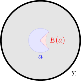
Figure 6: On a static slice $\Sigma$ of AdS, a causally complete region a and its entanglement wedge E(a), which includes the blue region as well. In $2+1$d, the dashed red line is a geodesic. In higher dimensions, it is a minimal surface.

3.5 Applications

Having determined our final entropy formula in (46), we now apply it to some examples. Let $\Sigma$ be asymptotically AdS or flat, and let $a$ have a single connected component. Additionally, assume the bulk matter fields are in their ground state and that $\Sigma$ is two dimensional, i.e., is a Cauchy slice for 2+1 dimensional spacetime. We will now show that $E(a)$ is the convex hull of $a$. First, note that it is sufficient to prove that any two points on $\partial E(a)$ are connected by a geodesic passing entirely through $E(a)$. Letting $p,q$ be two points on $\partial E(a)$, and $\gamma\subset E(a)$ the minimal length curve that connects $p$ to $q$ and is contained within $E(a)$. Additionally, let $\gamma^{\prime}$ be the unique geodesic connecting $p$ to $q$. If $\gamma\neq\gamma^{\prime}$, then we could decrease the boundary length of $E(a)$ by instead considering $E(a)^{\prime}$, defined by replacing $\gamma\to\gamma^{\prime}$ and filling in the space. This violates the minimality assumption of $E(a)$ unless $\gamma=\gamma^{\prime}$, and thus $E(a)$ is convex. A similar proof holds in higher dimensions by considering minimal area surfaces instead of curves. In higher dimensions, $E(a)$ may no longer be convex, but its boundary is still the minimal area surface containing $a$. This result is perhaps most surprising when $a$ is a thin spherical shell, as the region of minimal surface area containing the shell simply fills in the missing sphere in its interior.

In the de Sitter vacuum, however, $E(a)$ will expand to cover all of $\Sigma$, independent of the size of $a$ because the area will always be minimized by covering the whole space, as $\Sigma$ is compact. This implies that the entropy of de Sitter spacetimes is zero (in the renormalized sense of equation (21)) because the boundary of $E(a)$ is trivial. However, if we put an observer in the complementary patch of $a$, the constraints imposed by the observer may change this result. For example, if we model the observer as an excluded point from $a^{\prime}$, and provide sufficient entanglement between this observer and the rest of the complementary patch $a^{\prime}$, then $E(a)$ will minimize the generalized entropy by excluding $a^{\prime}$, implying a non-zero answer. This qualitatively matches balasubramanian2023sitter , and it would be interesting to see if making this observer more precise in our model reproduces the calculations of the entropy of de Sitter spacetimes in Chandrasekaran_2023 ; balasubramanian2023sitter .

4 Discussion

We proposed a path integral for finite gravitating regions and used it to argue that the entropy of an open region $A\subset\Sigma$ of a spacetime at a moment of time symmetry is determined by a (possibly larger) region $E(a)\subset\Sigma$ defined by: (1) $A\subseteq E(a)$, and (2) $E(a)$ minimizes the generalized entropy among all regions satisfying (1). This argument made no assumptions about the asymptotic structure of $\Sigma$ or the cosmological constant. For AdS/flat spacetimes without matter fields, $E(a)$ will simply be the minimal area surface containing $A$. In dS spacetimes, $E(a)$ will contain the whole Cauchy slice.

Several recent works have obtained results related to ours. In Folkestad:2023cze , it is argued that extremal surfaces and non-perturbative features of the background are sufficient structures to dress perturbations to allow for independence of subregions in quantum gravity. Our findings are consistent with this result. When $\partial A\neq\partial E(a)$, $\partial E(a)$ is extremal and dressing to this portion of the corner is allowed. On the other hand, if $\partial A=\partial E(a)$, then this portion of the corner is fixed to all orders in perturbation theory, i.e. it is nonperturbatively defined.

The authors of Dong_2020 define a notion of “effective entropy” for a subregion in a gravitating spacetime. However, they arrive at a different formula for the entropy, as they only consider area contributions when $\phi(a)$ contains a different number of components than $a$, i.e. only the area of islands. In contrast, we also have an area contribution from the original region $a$ as well. They do this to avoid singularities and ensure that the original region is the saddle in the $G_{N}\to 0$ limit. Additionally, they did not fully specify how to define a subregion in a gauge invariant way. We used the edge modes associated with $a$ to cure both of these issues, as we used the algebraic feature of the entangling product to ensure that the saddle $E(a)$ is on-shell, and the embedding map $\phi$ manifestly defined $a$ in a gauge invariant way.

Finally, in Jensen:2023yxy ; Chandrasekaran_2023 ; kudlerflam2023generalized the authors compute the entropy of a subregion in a gravitating spacetime by assuming the existence of an observer and dressing the fluctuations in $a$ to this observer. Using algebraic techniques such as the crossed product, they have all found that the algebra of observables undergoes a phase transition from type III, as is the case with local QFT, to type II, which has a well defined entropy up to an overall state-independent ambiguity. This is highly consistent with our renormalization scheme. As we have emphasized in the main text, there is a very suggestive analogy between the edge modes we consider here and the observers they consider. Roughly, they impose the constraint between the bulk fields and the edge modes for a subset of the edge modes with all transform in some subalgebra of the $\mathfrak{sl}(2,\mathbb{R})$ component of $\mathfrak{ecs}$. On the other hand, our main result of the larger region computing the entropy relied heavily on including the $\mathbb{R}^{2}$ component of $\mathfrak{ecs}$. This suggests that it is the $\mathfrak{sl}(2,\mathbb{R})$ part of $\mathfrak{ecs}$ which makes the entropy UV finite, and the $\mathbb{R}^{2}$ part which determines its actual value. The explicit construction of an algebraic picture connecting edge modes with the crossed product has been investigated in klinger2023crossed , and it would be interesting to make the connection of these results to our own more precise in future work.

4.1 The meaning of our construction: terrestrial holography?

Our formula for the entropy recalls the Ryu-Takayanagi (RT) formula in the AdS/CFT correspondence, which says that given a boundary subregion $R$ at a moment of time symmetry, the entropy in the field theory is given by the minimal area surface homologous to $R$ Ryu_2006 . In fact, in the case that $\Sigma$ is asymptotically AdS and $a$ approaches a boundary subregion, our prescription for computing the entropy in the $G_{N}\to 0$ limit precisely matches the RT formula. In AdS/CFT, the RT formula was justified via the gravitational path integral Lewkowycz_2013 , similarly to our approach. It is surprising that the gravitational path integral, defined on inherently coarse grained degrees of freedom, is sufficient to derive a microscopic entropy formula, which seems like it would need non-perturbative control to compute. For the entropy of black holes, recent work Penington:2019kki ; Balasubramanian:2022gmo has clarified why the gravitational path integral may actually contain information about the microscopic density of states. It would be useful to understand whether some similar insight applies to the the RT formula and to our results.

We know that the RT formula is about more than just entropy: it also determines the bulk information in the gravitating theory that is localized within various subregions of the dual boundary theory. Specifically, given a boundary subregion $R$, and its associated entanglement wedge $E(R)$, any bulk operator with support on $E(R)$ can be reconstructed in the boundary using operators solely living in $R$ Almheiri_2015 . This property is called entanglement wedge reconstruction (EWR) and arises entirely from the fact that the RT formula computes entanglement entropy, and the resulting quantum information constraints on holographic encoding of information. The RT formula satisfies many non-trivial consistency checks, which motivated EWR in the first place, such as no-cloning, nesting, and strong sub-additivity. Does our proposal for the entropy of a bulk subregion pass the same tests?

In fact, Bousso and Penington recently conjectured BP_static that the entropy of a bulk region $a$ at a moment of time symmetry satisfies equation (46), and so our work can be seen as evidence for their proposal. They demonstrated that a region $E(a)$ that satisfies the conditions arising from our analysis of the path integral for finite regions does satisfy no-cloning, nesting, and strong sub-additivity. Indeed, this is why they proposed that it computed the entropy. Their result is highly suggestive that the bulk saddle $E(a)$ really is computing an entanglement entropy, as opposed to merely computing a coarse-grained entropy. In AdS/CFT, these entangled degrees of freedom are thought to be those of a CFT living on the spacetime boundary. However, these boundary degrees of freedom can be defined through the extrapolate dictionary banks1998ads ; Balasubramanian:1999ri ; Hamilton:2006az ; harlow2011operator . Thus, not only is the bulk defined by the boundary theory, but the boundary is defined by the bulk theory. It is therefore natural to ask if one can view holographic encoding not as a map from the bulk to the boundary, but also as a map from the bulk to other bulk subregions. Indeed, this is the scenario proposed in BP_static ; bousso2023holograms and also suggested by our entropy computation.

We can further motivate a notion of bulk-to-bulk holography as follows, using the scenarios outlined in BP_static . Sticking to AdS spacetimes, where the dual theory is better understood, let $a_{\epsilon}$ be a spherical band containing the asymptotic boundary and with radius $\rho=\epsilon$ in global coordinates, as in Fig. 7. Full knowledge of the theory of quantum gravity within $a_{\epsilon}$ includes full knowledge of the asymptotic boundary by the extrapolate dictionary. Because the entanglement wedge of the entire boundary is the entire spacetime, this suggests that in the full theory of gravity, $a_{\epsilon}$ encodes the full slice $\Sigma$ as well. In fact, this argument generalizes to any bulk region $a_{R}$ which contains a boundary subregion $R$, i.e. $a_{R}$ should encode all of $E(R)$ as well, even though it is a bulk region. Furthermore, consider a spacetime containing an evaporating black hole. If the Hawking radiation is collected in an external reservoir, one can show that the interior of the black hole is encoded in the Hawking radiation after the Page time Marolf_2021 ; Penington:2019kki ; Almheiri:2019hni ; Hartman_2020 . Specifically, an “island” behind the black hole horizon is holographically encoded in the distant radiation. But now suppose that the Hawking radiation does not escape to the reservoir, but instead is collected at a finite but large distance from the black hole, say in the memory bank of a quantum computer. Performing the same quantum computations as if the radiation were in the reservoir, we expect that the interior is still encoded within the Hawking radiation, i.e., that “escaping past infinity” is not actually crucial to the physics of information recovery through entanglement islands. But because the Hawking radiation is still localized within the bulk, it would appear that we should view the island as an entanglement wedge for the quantum computer, a finite region within the gravitating system. Finally, this idea of a bulk-to-bulk encoding has motivations in tensor network models of quantum gravity BP_static ; Pastawski_2015 .

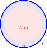
Figure 7: A bulk subregion of AdS with complete information about the boundary can reconstruct the entire spacetime.

For more examples, consider the case when $a$ is a star shaped region, an example of which is shown in Fig. 8, smoothing out the sharp kinks in $\partial a$ as needed. Similarly to the example shown in Fig. 6, $E(a)$ will fill out the gaps between the “legs” of the star. However, consider a second region $b$, which is taken to be thin-but-finite shell with outer boundary $\partial E(a)$. In other words, $b$ is the intersection of $E(a)$ and a small open neighborhood of $\partial E(a)$. Then by construction, $E(a)=E(b)$, despite the fact that $a\cap b$ can be arbitrarily small. This suggests that $a$ and $b$ both contain the “same information”, despite being quite distinct geometrically. Understanding the consistency of these two representations of $E(a)$ will clearly require non-trivial quantum error correcting properties of the map between $a,b$ to $E(a)$. Finally, we argued in Sec. 3.5 that for any closed universe with a moment of time symmetry, any open set $a$ has $E(a)=\Sigma$, which suggests that any open set of a closed universe has complete information about the entire spacetime. This is very similar to what was found in chakraborty2023holography , but it is important to note that they obtained this result by studying the Hilbert space associated to a late/early time Cauchy slice, as opposed to the finite time static slice we consider in this paper. Assuming that $E(a)$ defined in our paper is truly analogous to an entanglement wedge, the same result holds in essentially two opposite regimes, providing evidence that this strange feature of closed universes is true for all times.

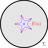
Figure 8: A star shaped region $a$ in the AdS vacuum, which should be smoothed out near any kinks. It has arbitrarily small overlap with $b:=\mathcal{B}_{\epsilon}(\partial E(a))$, an open neighborhood of the corner of E(a). Because $E(a)=E(b)$, these two regions have the same entropy despite being quite distinct geometrically.

Another check of our proposal in AdS comes from previous works Balasubramanian:2013rqa ; Balasubramanian_2014 ; Myers_2014 which have investigated the entropy of a finite region of spacetime by exploiting the purity of the global state $\ket{\Psi}$ and computing the “differential entropy” associated to a time band outside the region. A puzzle in these calculations involved the treatment of non-convex regions Czech:2015qta ; ju2023generalized ; ju2023squashed , as the time bands they construct will always have a convex Rindler horizon. Our calculation suggests a potential resolution to this puzzle in $2+1$ dimensions. Let $a$ be a non-convex gravitating region in $2+1$d with entanglement wedge $E(a)$. If we assume that the system satisfies complementary recovery, then the complementary degrees of freedom are captured by $E(a)^{\prime}$, namely the points in $\Sigma$ outside $E(a)$. But $E(a)$ is the convex hull of $a$, and so the domain of dependence $D[E(a)^{\prime}]$ has precisely of the form of the time bands studied in Balasubramanian_2014 ; Myers_2014 . This implies that the entropy of $a$ is equal to the entropy of the time band, a requirement for the global state to be pure. If the entropy of $a$ was the area of $a$ and not $E(a)$, this would not have been the case.

Finally, return to the case mentioned in Sec. 3.5 of a thin spherical shell. Our entropy formula suggests that all the degrees of freedom in a compact region of space $a$ live at an open neighborhood of the boundary of $E(a)$. This is reminiscent of the original conception of the holographic principle by ’t Hooft and Susskind hooft2009dimensional ; Susskind_1995 . These examples strongly motivate the existence of a more “terrestrial” formulation of holography, where the dual degrees of freedom are located “closer to us” within compact regions of the gravitating spacetime, as opposed to “the heavens” at asymptotic infinity. It would be very interesting to more precisely define this “dual theory”.

Acknowledgments:

We thank Jon Sorce, Jonah Kudler-Flamm, Anthony Speranza, Sam Leutheusser, and Gautam Satishchandran for detailed comments on an early version of this paper. We are also grateful to Chitraang Murdia, Onkar Parrikar, Bartek Czech, Wayne Weng, Roberto Emparan, Rob Myers, Suvrat Raju, Raphael Bousso, and Rob Leigh for useful conversations and communications. VB is supported by the DOE through DE-SC0013528 and the QuantISED grant DE-SC0020360. CC is supported by the National Science Foundation Graduate Research Fellowship under Grant No. DGE-2236662. VB and CC thank the Yukawa Institute at the University of Kyoto for hospitality during the YITP-T-23-01 Quantum Information, Quantum Matter and Quantum Gravity workshop.

References

- (1) J.D. Bekenstein, Black holes and entropy, Phys. Rev. D 7 (1973) 2333.
- (2) S.W. Hawking, Particle creation by black holes, Communications in Mathematical Physics 43 (1975) 199 .
- (3) G.W. Gibbons and S.W. Hawking, Cosmological Event Horizons, Thermodynamics, and Particle Creation, Phys. Rev. D 15 (1977) 2738.
- (4) T. Jacobson and R. Parentani, Horizon entropy, Foundations of Physics 33 (2003) 323–348.
- (5) W.G. Unruh, Notes on black hole evaporation, Phys. Rev. D 14 (1976) 870.
- (6) T. Jacobson, Thermodynamics of spacetime: The einstein equation of state, Physical Review Letters 75 (1995) 1260–1263.
- (7) S. Ryu and T. Takayanagi, Holographic derivation of entanglement entropy from the anti–de sitter space/conformal field theory correspondence, Physical Review Letters 96 (2006) .
- (8) T. Faulkner, A. Lewkowycz and J. Maldacena, Quantum corrections to holographic entanglement entropy, JHEP 11 (2013) 074 [1307.2892].
- (9) V.E. Hubeny, M. Rangamani and T. Takayanagi, A Covariant holographic entanglement entropy proposal, JHEP 07 (2007) 062 [0705.0016].
- (10) N. Engelhardt and A.C. Wall, Quantum Extremal Surfaces: Holographic Entanglement Entropy beyond the Classical Regime, JHEP 01 (2015) 073 [1408.3203].
- (11) R. Bousso and G. Penington, Entanglement wedges for gravitating regions, Physical Review D 107 (2023) .
- (12) R. Bousso and G. Penington, Holograms in our world, Phys. Rev. D 108 (2023) 046007.
- (13) J. Maldacena, The large n limit of superconformal field theories and supergravity, International Journal of Theoretical Physics 38 (1999) 1113–1133.
- (14) S. Pasterski, M. Pate and A.-M. Raclariu, Celestial holography, 2111.11392.
- (15) S. Pasterski, Lectures on celestial amplitudes, The European Physical Journal C 81 (2021) .
- (16) A. Strominger, Lectures on the infrared structure of gravity and gauge theory, 1703.05448.
- (17) A.-M. Raclariu, Lectures on celestial holography, 2107.02075.
- (18) A. Strominger, The ds/cft correspondence, Journal of High Energy Physics 2001 (2001) 034–034.
- (19) V. Balasubramanian, J. de Boer and D. Minic, Mass, entropy and holography in asymptotically de Sitter spaces, Phys. Rev. D 65 (2002) 123508 [hep-th/0110108].
- (20) E. Witten, Quantum gravity in de sitter space, hep-th/0106109.
- (21) T. Chakraborty, J. Chakravarty, V. Godet, P. Paul and S. Raju, The Hilbert space of de Sitter quantum gravity, 2303.16315.
- (22) A. Almheiri, X. Dong and D. Harlow, Bulk locality and quantum error correction in ads/cft, Journal of High Energy Physics 2015 (2015) .
- (23) R. Haag, Local quantum physics: Fields, particles, algebras (1992).
- (24) W. Donnelly, Decomposition of entanglement entropy in lattice gauge theory, Physical Review D 85 (2012) .
- (25) H. Casini, M. Huerta and J.A. Rosabal, Remarks on entanglement entropy for gauge fields, Physical Review D 89 (2014) .
- (26) W. Donnelly and L. Freidel, Local subsystems in gauge theory and gravity, Journal of High Energy Physics 2016 (2016) .
- (27) C. Vafa, Quantum Symmetries of String Vacua, Mod. Phys. Lett. A 4 (1989) 1615.
- (28) R. Dijkgraaf, C. Vafa, E.P. Verlinde and H.L. Verlinde, The Operator Algebra of Orbifold Models, Commun. Math. Phys. 123 (1989) 485.
- (29) V. Chandrasekaran, R. Longo, G. Penington and E. Witten, An algebra of observables for de sitter space, Journal of High Energy Physics 2023 (2023) .
- (30) F. Peter and H. Weyl, Die vollständigkeit der primitiven darstellungen einer geschlossenen kontinuierlichen gruppe, Math. Ann. 97 (1927) .
- (31) L. Ciambelli and R. G. Leigh, Universal corner symmetry and the orbit method for gravity, Nuclear Physics B 986 (2023) 116053.
- (32) L. Freidel, R. Oliveri, D. Pranzetti and S. Speziale, Extended corner symmetry, charge bracket and einstein’s equations, Journal of High Energy Physics 2021 (2021) .
- (33) L. Ciambelli, R.G. Leigh and P.-C. Pai, Embeddings and integrable charges for extended corner symmetry, Physical Review Letters 128 (2022) .
- (34) H. Geng, Open ads/cft via a double trace deformation, 2023.
- (35) L. Ciambelli and R.G. Leigh, Isolated surfaces and symmetries of gravity, Physical Review D 104 (2021) .
- (36) A.-C. de la Hamette, T.D. Galley, P.A. Hoehn, L. Loveridge and M.P. Mueller, Perspective-neutral approach to quantum frame covariance for general symmetry groups, 2110.13824.
- (37) J.-P. Pier, “Amenable locally compact groups.” Pure and Applied Mathematics. A Wiley-Interscience Publication. New York etc.: John Wiley & Sons. X, 418 p. £ 49.80 (1984)., 1984.
- (38) X. Dong, S. McBride and W.W. Weng, Holographic tensor networks with bulk gauge symmetries, 2309.06436.
- (39) E. Gesteau, Large von neumann algebras and the renormalization of newton’s constant, 2302.01938.
- (40) S. Leutheusser and H. Liu, Subalgebra-subregion duality: emergence of space and time in holography, 2212.13266.
- (41) E. Witten, Gravity and the crossed product, Journal of High Energy Physics 2022 (2022) .
- (42) K. Jensen, J. Sorce and A. Speranza, Generalized entropy for general subregions in quantum gravity, 2306.01837.
- (43) J. Kudler-Flam, S. Leutheusser and G. Satishchandran, Generalized Black Hole Entropy is von Neumann Entropy, 2309.15897.
- (44) H. Geng, Revisiting recent progress in the karch-randall braneworld, 2023.
- (45) T. Jacobson, Entanglement equilibrium and the einstein equation, Physical Review Letters 116 (2016) .
- (46) M.S. Klinger and R.G. Leigh, Crossed products, extended phase spaces and the resolution of entanglement singularities, 2306.09314.
- (47) C. Akers and P. Rath, Holographic renyi entropy from quantum error correction, Journal of High Energy Physics 2019 (2019) .
- (48) X. Dong, D. Harlow and D. Marolf, Flat entanglement spectra in fixed-area states of quantum gravity, Journal of High Energy Physics 2019 (2019) .
- (49) D. Harlow, The ryu–takayanagi formula from quantum error correction, Communications in Mathematical Physics 354 (2017) 865–912.
- (50) A.J. Speranza, Local phase space and edge modes for diffeomorphism-invariant theories, Journal of High Energy Physics 2018 (2018) .
- (51) R.M. Wald, Black hole entropy is the noether charge, Physical Review D 48 (1993) R3427–R3431.
- (52) V. Iyer and R.M. Wald, Some properties of the noether charge and a proposal for dynamical black hole entropy, Physical Review D 50 (1994) 846–864.
- (53) V. Iyer and R.M. Wald, Comparison of the noether charge and euclidean methods for computing the entropy of stationary black holes, Physical Review D 52 (1995) 4430–4439.
- (54) M.S. Klinger, R.G. Leigh and P.-C. Pai, Extended phase space in general gauge theories, 2303.06786.
- (55) J. Kastikainen and A. Svesko, Gravitational rényi entropy from corner terms, 2312.06765.
- (56) X. Dong, A. Lewkowycz and M. Rangamani, Deriving covariant holographic entanglement, Journal of High Energy Physics 2016 (2016) .
- (57) L. Freidel, M. Geiller and W. Wieland, Corner symmetry and quantum geometry, 2302.12799.
- (58) A. Lewkowycz and J. Maldacena, Generalized gravitational entropy, Journal of High Energy Physics 2013 (2013) .
- (59) V. Balasubramanian, Y. Nomura and T. Ugajin, de sitter space is sometimes not empty, 2308.09748.
- (60) A. Folkestad, Subregion Independence in Gravity, 2311.09403.
- (61) X. Dong, X.-L. Qi, Z. Shangnan and Z. Yang, Effective entropy of quantum fields coupled with gravity, Journal of High Energy Physics 2020 (2020) .
- (62) G. Penington, S.H. Shenker, D. Stanford and Z. Yang, Replica wormholes and the black hole interior, JHEP 03 (2022) 205 [1911.11977].
- (63) V. Balasubramanian, A. Lawrence, J.M. Magan and M. Sasieta, Microscopic origin of the entropy of black holes in general relativity, 2212.02447.
- (64) D.L. Jafferis, A. Lewkowycz, J. Maldacena and S.J. Suh, Relative entropy equals bulk relative entropy, Journal of High Energy Physics 2016 (2016) .
- (65) C.-F. Chen, G. Penington and G. Salton, Entanglement wedge reconstruction using the petz map, Journal of High Energy Physics 2020 (2020) .
- (66) T. Banks, M.R. Douglas, G.T. Horowitz and E.J. Martinec, AdS dynamics from conformal field theory, hep-th/9808016.
- (67) V. Balasubramanian, S.B. Giddings and A.E. Lawrence, What do CFTs tell us about Anti-de Sitter space-times?, JHEP 03 (1999) 001 [hep-th/9902052].
- (68) A. Hamilton, D.N. Kabat, G. Lifschytz and D.A. Lowe, Holographic representation of local bulk operators, Phys. Rev. D 74 (2006) 066009 [hep-th/0606141].
- (69) D. Harlow and D. Stanford, Operator Dictionaries and Wave Functions in AdS/CFT and dS/CFT, 1104.2621.
- (70) D. Marolf and H. Maxfield, Observations of hawking radiation: the page curve and baby universes, Journal of High Energy Physics 2021 (2021) .
- (71) A. Almheiri, R. Mahajan, J. Maldacena and Y. Zhao, The Page curve of Hawking radiation from semiclassical geometry, JHEP 03 (2020) 149 [1908.10996].
- (72) T. Hartman, Y. Jiang and E. Shaghoulian, Islands in cosmology, Journal of High Energy Physics 2020 (2020) .
- (73) F. Pastawski, B. Yoshida, D. Harlow and J. Preskill, Holographic quantum error-correcting codes: toy models for the bulk/boundary correspondence, Journal of High Energy Physics 2015 (2015) .
- (74) T. Chakraborty, J. Chakravarty, V. Godet, P. Paul and S. Raju, Holography of information in de sitter space, 2023.
- (75) V. Balasubramanian, B. Czech, B.D. Chowdhury and J. de Boer, The entropy of a hole in spacetime, JHEP 10 (2013) 220 [1305.0856].
- (76) V. Balasubramanian, B.D. Chowdhury, B. Czech, J. de Boer and M.P. Heller, Bulk curves from boundary data in holography, Physical Review D 89 (2014) .
- (77) R.C. Myers, J. Rao and S. Sugishita, Holographic holes in higher dimensions, Journal of High Energy Physics 2014 (2014) .
- (78) B. Czech, L. Lamprou, S. McCandlish and J. Sully, Integral Geometry and Holography, JHEP 10 (2015) 175 [1505.05515].
- (79) X.-X. Ju, W.-B. Pan, Y.-W. Sun and Y.-T. Wang, Generalized rindler wedge and holographic observer concordance, 2302.03340.
- (80) X.-X. Ju, B.-H. Liu, W.-B. Pan, Y.-W. Sun and Y.-T. Wang, Squashed entanglement from generalized rindler wedge, 2310.09799.
- (81) G. ’t Hooft, Dimensional reduction in quantum gravity, gr-qc/9310026.
- (82) L. Susskind, The world as a hologram, Journal of Mathematical Physics 36 (1995) 6377–6396.