Transition of Anticoncentration in Gaussian Boson Sampling

Abstract

Gaussian Boson Sampling is a promising method for experimental demonstrations of quantum advantage because it is easier to implement than other comparable schemes. While most of the properties of Gaussian Boson Sampling are understood to the same degree as for these other schemes, we understand relatively little about the statistical properties of its output distribution. The most relevant statistical property, from the perspective of demonstrating quantum advantage, is the anticoncentration of the output distribution as measured by its second moment. The degree of anticoncentration features in arguments for the complexity-theoretic hardness of Gaussian Boson Sampling, and it is also important to know when using cross-entropy benchmarking to verify experimental performance. In this work, we develop a graph-theoretic framework for analyzing the moments of the Gaussian Boson Sampling distribution. Using this framework, we show that Gaussian Boson Sampling undergoes a transition in anticoncentration as a function of the number of modes that are initially squeezed compared to the number of photons measured at the end of the circuit. When the number of initially squeezed modes scales sufficiently slowly with the number of photons, there is a lack of anticoncentration. However, if the number of initially squeezed modes scales quickly enough, the output probabilities anticoncentrate weakly.

There is a hope that quantum computation will be able to outperform classical computation on certain tasks. In particular, there has been a recent explosion of interest in so-called sampling problems given the strong theoretical evidence for an exponential speedup of quantum algorithms over the best possible classical algorithms; see Ref. Hangleiter and Eisert (2023) for an overview. Aaronson and Arkhipov introduced one of the most deeply studied sampling frameworks in their seminal work on Boson Sampling Aaronson and Arkhipov (2013). The Boson Sampling task is to approximately sample from the outcome distribution of measuring $n$ single photons in $m$ optical modes transformed by a Haar-random linear-optical unitary, which can be implemented as a random network of beamsplitters and phase shifters Reck et al. (1994). Aaronson and Arkhipov (2013) focused on single-photon input states, but these can be challenging to produce experimentally Wang et al. (2019) because existing single-photon sources are not sufficiently reliable to avoid an exponential amount of post-selection Brod et al. (2019). Therefore, there has been an interest in generalizing the original Boson Sampling setup to other input states.

The currently most feasible generalization is Gaussian Boson Sampling (GBS) Lund et al. (2014); Rahimi-Keshari et al. (2015); Hamilton et al. (2017); Kruse et al. (2019), which uses Gaussian input states. These states are significantly easier to prepare reliably than single-photon states. At the same time, similar statements can be made about the hardness of sampling from the corresponding output distribution Kruse et al. (2019); Deshpande et al. (2022a); Grier et al. (2022); Chabaud and Walschaers (2023), and several large-scale GBS experiments have been performed recently Zhong et al. (2020, 2021); Madsen et al. (2022); Deng et al. (2023).

Broadly speaking, the hardness of Boson Sampling is based on the connection between output probabilities and the permanent, which is, classically, $\#\mathsf{P}$-hard to compute Valiant (1979). Similarly, the hardness of GBS arises from the fact that output probabilities are controlled by a generalization of the permanent called the hafnian; while the permanent counts the number of perfect matchings in a weighted bipartite graph, the hafnian counts the number of perfect matchings in an arbitrary weighted graph. Because the hafnian generalizes the permanent, it is also difficult to compute classically.

However, the complexity of classically computing an individual output probability defined in terms of the permanent or the hafnian is not itself sufficient to prove hardness of sampling from the overall probability distributions. The standard hardness argument based on Stockmeyer’s algorithm Stockmeyer (1983); Hangleiter and Eisert (2023) requires that outcome probabilities of random Boson Sampling instances be hard to approximate. Jointly with provable hardness of nearly exactly computing output probabilities Deshpande et al. (2022a), anticoncentration of the outcome probabilities serves as evidence for this. Intuitively, if most outcome probabilities are comparable to the uniform probability, then a good classical sampling algorithm needs a very precise idea of each probability’s relative magnitude because all of them are important. Anticoncentration quantifies this idea as, most concisely, the outcome-collision probability (i.e. the probability of getting the same outcome from two independent samples) of the GBS distribution averaged over the choice of linear-optical unitary and normalized by the size of the effective sample space (Hangleiter and Eisert, 2023, Sec. D). While a weak form of anticoncentration holds in Boson Sampling Aaronson and Arkhipov (2013), under what conditions anticoncentration holds in GBS is an open question.

In this work, we analyze the moments of GBS in the photon-collision-free limit. In this limit, the output distribution is dominated by outcomes with at most a single photon in each mode, and the moments of GBS approximately reduce to moments of squared hafnians of Gaussian random matrices. We show that evaluating those moments reduces to counting the connected components of certain graphs. Using this perspective, we find a closed-form expression for the first moment and derive analytical properties of the second moment. We then identify a transition in anticoncentration in GBS: when the number of initially squeezed modes is large enough compared to the measured number of photons $n$, a weak version of anticoncentration holds where the normalized average outcome-collision probability scales as $\sqrt{n}$. However, when sufficiently few modes are initially squeezed, there is a lack of anticoncentration, as the normalized second moment scales exponentially in $n$.

The rest of the paper proceeds as follows. We first provide background information and set up the system and problem of interest. We then derive the graph-theoretic formalism for computing the first moment of the output probabilities. We proceed to discuss how to apply the formalism to calculate certain properties of the second moment. These results let us finally prove the transition in anticoncentration.

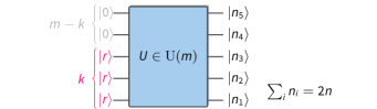
Figure 1: In Gaussian Boson Sampling (GBS), $k$ out of $m$ modes are prepared in single-mode squeezed states with parameter $r$, while the remaining modes are prepared in the vacuum state $\ket{0}$. The modes are then transformed by a Haar random linear-optical unitary $U$ and measured in the Fock basis with outcome counts $n_{i}$ summing to $2n$.

Setup.—We consider a photonic system with $m$ modes that is transformed by a Haar-random linear optical unitary $U\in\mathrm{U}(m)$ acting on the modes of the system, see Fig. 1. In the paradigmatic version of GBS Hamilton et al. (2017); Kruse et al. (2019), the first $k$ of the $m$ modes are prepared in single-mode squeezed states with equal squeezing parameter $r$, while the remaining $m-k$ modes are prepared in the vacuum state. After applying $U$, all $m$ modes are measured in the Fock basis.

Reference Hamilton et al. (2017) proves that, given a unitary $U$, the probability of obtaining an outcome count vector $\mathbf{n}=(n_{1},n_{2},\ldots,n_{m})\in\mathbb{N}_{0}^{m}$ with total photon count $2n=\sum_{i=1}^{m}n_{i}$ is given by

$$P_{U}(\mathbf{n})=\frac{\tanh^{2n}r}{\cosh^{k}r}\absolutevalue{\mathrm{Haf}(U^{\top}_{1_{k},\mathbf{n}}U_{1_{k},\mathbf{n}})}^{2},$$ (1)

where $U_{1_{k},\mathbf{n}}$ denotes the $k\times 2n$ submatrix of $U$ given by its first $k$ rows and the columns selected according to the nonzero entries of $\mathbf{n}$ each copied $n_{i}$ times . Moreover,

$$\mathrm{Haf}(A)=\frac{1}{2^{n}n!}\sum_{\sigma\in S_{2n}}\prod_{j=1}^{n}A_{\sigma(2j-1),\sigma(2j)}$$ (2)

denotes the hafnian of a $2n\times 2n$ symmetric matrix $A$ .

We will work in the regime in which the output states are, with high probability, (photon-)collision-free, meaning that $n_{i}\in\{0,1\}$ for all $i$. A sufficient condition for this to be the case is that the expected number of photons $\operatorname*{\mathbb{E}}[2n]=k\sinh^{2}(r)=o(\sqrt{m})$. In this regime, Ref. Deshpande et al. (2022a) provides evidence that, for any fixed $n=o(\sqrt{m})$, the distribution over submatrices is well-captured by a generalization of the circular orthogonal ensemble (COE) .

Conjecture 1 (Hiding Deshpande et al. (2022a)).

For any $k$ such that $1\leq k\leq m$ and $2n=o(\sqrt{m})$, the distribution of the symmetric product $U^{\top}_{1_{k},\mathbf{n}}U_{1_{k},\mathbf{n}}$ of submatrices of a Haar-random $U\in\mathrm{U}(m)$ closely approximates in total variation distance the distribution of the symmetric product $X^{\top}X$ of a complex Gaussian matrix $X~{}\sim~{}\mathcal{N}(0,1/m)_{c}^{k\times 2n}$ with mean $0$ and variance $1/m$.

We work under the assumption that Conjecture 1 is true. Fixing the measured number of photons $2n$, the normalized average (outcome-)collision probability, which quantifies anticoncentration, can be written as $|\Omega_{2n}|\operatorname*{\mathbb{E}}_{U\in U(m)}[\sum_{\mathbf{n}\in\Omega}P_{U}(\mathbf{n})^{2}]$, where $|\Omega_{2n}|$ is the size of the effective sample space. Conjecture 1 implies that, with respect to random choices of $U$, all outcomes are equally distributed over the unitaries, the so-called hiding property. This implies that the inverse size of the (effective) sample space is given by the first moment $\mathbb{E}_{U}[P_{U}(\mathbf{n})]$ . Under Conjecture 1, the anticoncentration property thus reduces to computing the moments

$$M_{t}(k,n)\coloneqq\operatorname*{\mathbb{E}}_{X\sim\mathcal{G}^{k\times 2n}}[|\mathrm{Haf}(X^{\top}X)|^{2t}]$$ (3)

of the squared hafnian as a function of the parameters $k$ and $n$ for $t=1,2$, where we have abbreviated $\mathcal{N}(0,1)_{c}^{k\times 2n}$ as $\mathcal{G}^{k\times 2n}$. We consider unit variance because rescaling $X$ by $1/\sqrt{m}$ just leads to an overall prefactor that, like the prefactor in Eq. 1, is irrelevant to the normalized average outcome-collision probability. We will phrase our discussion in terms of the inverse of the average collision probability

$$m_{2}(k,n)\coloneqq M_{1}(k,n)^{2}/M_{2}(k,n).$$ (4)

First moment and graph-theoretic formalism.—We begin by analyzing the (rescaled) first moment $M_{1}$ of the output probabilities. In order to derive our graph-theoretic formalism, we use Eq. 2 to expand the hafnian in Eq. 3 as a sum over permutations of a product of matrix elements. From there, the key is to use that the matrix elements are independent complex Gaussian, meaning that $\mathbb{E}_{X\sim\mathcal{G}^{k}}[X_{i}X^{*}_{j}]=\delta_{ij}$ and $\mathbb{E}_{X\sim\mathcal{G}^{k}}[X_{i}X_{j}]=\mathbb{E}_{X\sim\mathcal{G}^{k}}[X^{*}_{i}X^{*}_{j}]=0$. This yields

$$M_{1}(k,n)=\frac{(2n)!}{(2^{n}n!)^{2}}\sum_{\tau\in S_{2n}}\sum_{\{o_{i}\}_{i=1}^{n}}^{k}\prod_{j=1}^{n}\delta_{o_{\left\lceil\frac{\tau(2j-1)}{2}\right\rceil}o_{\left\lceil\frac{\tau(2j)}{2}\right\rceil}},$$ (5)

see the Supplemental Material (SM) for details.

Let us briefly discuss Eq. 5. The sum over $\tau\in S_{2n}$ and the product over index $j$ come from the definition (2); the sum over the indices $o_{i}\in[k]\coloneqq\{1,2,\ldots,k\}$ is due to an expansion of $X^{\top}X$ as a matrix product. Note that, when $\tau(2j-1)$ and $\tau(2j)$ form a tuple $(2\ell-1,2\ell)$, then the Kronecker $\delta$ always equals $1$ for index $o_{\ell}$, such that summing over $o_{\ell}$ yields a factor of $k$. When $\tau(2j-1)$ and $\tau(2j)$ do not form such a tuple, we get a nontrivial relationship between the indices that decreases the number of independent degrees of freedom, thus decreasing the number of factors of $k$ in the final answer. Therefore, to evaluate this expression, one must determine the number of “free indices” over all the permutations in $S_{2n}$. We accomplish this with our graph-theoretic approach.

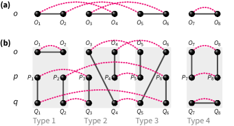
Figure 2: Examples of graphs used to calculate the (a) first and (b) second moments of GBS outcome probabilities. (a) $G\in\mathbb{G}^{1}_{4}$. There are eight vertices $O_{1}$ to $O_{8}$ representing the index $o$ (labeled in the left column). The black (solid) edges connect only adjacent pairs, whereas the red (dashed) edges form an arbitrary perfect matching. This graph has two connected components, meaning it would contribute $k^{2}$ to the first moment. (b) $G\in\mathbb{G}_{4}^{2}$. The black (solid) edges are, from left to right, type-1, type-2, type-3, and type-4, as denoted by the gray background. This means that $z=1+0\times 4^{0}+1\times 4^{1}+2\times 4^{2}+3\times 4^{3}=229$ (this is calculated by converting 0123 from base-4 into base-10 and then adding 1 such that the final result is in $[4^{4}]$). Note that black (solid) edges stay within two adjacent columns. Red (dashed) edges form an arbitrary perfect matching in each row. This graph contributes $k^{5}$ to the second moment, as there are five connected components.

Specifically, define a graph $G_{\tau}$ as follows, see Fig. 2(a). Let $G_{\tau}$ have $2n$ vertices labeled $O_{1}$ through $O_{2n}$. These upper-case vertices are not directly equivalent to the lower-case indices in Eq. 5—instead, each index $o_{j}$ splits into two vertices $O_{\ell}$ and $O_{\ell^{\prime}}$ such that $\lceil\tau(\ell)/2\rceil=j=\lceil\tau(\ell^{\prime})/2\rceil$. Let $G_{\tau}$ have a black edge between $O_{2j-1}$ and $O_{2j}$ for all $j\in[n]$, and a red edge between $O_{\ell}$ and $O_{\ell^{\prime}}$ if $\lceil\tau(\ell)/2\rceil=\lceil\tau(\ell^{\prime})/2\rceil$. These two kinds of edges mimic two types of ways that dependencies in Eq. 5 can be induced through an index $j$. Red edges identify the $\ell$ and $\ell^{\prime}$ that map to the same value via $\tau$ and the ceiling function, hence red edges identify which vertices came from the same $o$ index. Black edges identify that the images of $2j-1$ and $2j$ are always linked by a Kronecker $\delta$.

We see, then, that the number of connected components of $G_{\tau}$, $C(G_{\tau})$, is equivalent to the number of free indices in the sum in Eq. 5. Therefore,

$$M_{1}(k,n)=\frac{(2n)!}{\left(2^{n}n!\right)^{2}}\sum_{\tau\in S_{2n}}k^{C(G_{\tau})}.$$ (6)

Now, there is a degeneracy where many permutations induce the same final graph. Each graph has the same fixed set of black edges and then one of $(2n-1)!!$ possible sets of red edges (this is the number of ways of pairing $2n$ elements when order does not matter). For each graph $G$ corresponding to some assignment of the red edges, there are $2^{n}n!$ permutations $\tau$ such that $G_{\tau}=G$. Therefore, instead of studying $G_{\tau}$ as instantiated by permutations $\tau$, we study the underlying graphs $G$. Define $\mathbb{G}^{1}_{n}$ to be the set of graphs on $2n$ vertices with one perfect matching defined by the fixed set of black edges and one perfect matching defined by the arbitrary red edges. We can thus rewrite $M_{1}=(2n-1)!!\sum_{G\in\mathbb{G}^{1}_{n}}k^{C(G)}$ and state our first result.

Theorem 1.

The sum over graphs in $\mathbb{G}^{1}_{n}$ satisfies

$$\sum_{G\in\mathbb{G}^{1}_{n}}k^{C(G)}=k(k+2)\dots(k+2n-2),$$ (7)

and hence $M_{1}(k,n)=(2n-1)!!(k+2n-2)!!/(k-2)!!$.

The proof proceeds by induction over $n$, where the inductive step reduces a graph in $\mathbb{G}_{n}^{1}$ to one in $\mathbb{G}_{n-1}^{1}$ through an analysis of the red edge connected to $O_{1}$. There are two options for this red edge: either it connects to $O_{2}$, the vertex with which $O_{1}$ shares a black edge, or it attaches to some $O_{a>2}$. The former creates a connected component of size two; the latter reduces to a graph in $\mathbb{G}_{n-1}^{1}$ by merging vertices $O_{1}$, $O_{2}$, and $O_{a}$ (which does not change the number of connected components). Full details can be found in the SM.

Second Moment.—We now sketch the application of our graph-theoretic formalism to the second moment $M_{2}$, deferring the details to the SM. We expand $\absolutevalue{\mathrm{Haf}(X^{\top}X)}^{4}$ using Eq. 2 which becomes a sum of products of matrix elements that are indexed by four permutations in $S_{2n}$. The independence of matrix elements again ensures that we must have an equal number of copies of $X_{ij}$ and $X_{ij}^{*}$ for the expectation value not to vanish on a given product. However, because there are more copies of $X$, there are more ways of matching the indices. Accounting for these possibilities leads to an expression analogous to Eq. 5. The key differences are the following: (1) instead of summing over a single permutation, we now sum over three permutations, labeled $\tau,\alpha,\beta$ (as in the first moment, one of the original four permutations eventually becomes redundant); (2) instead of summing over $n$ indices $\{o_{i}\}_{i=1}^{n}$, we now sum over $3n$ indices $\{o_{i},q_{i},p_{i}\}_{i=1}^{n}$; (3) each factor is a sum of four possible Kronecker $\delta$ terms corresponding to the different types of index matching.

As before, we will define a useful set of graphs; see Fig. 2(b) for an example. We expand each index in $\{o_{i},q_{i},p_{i}\}_{i=1}^{n}$ to two graph vertices $\{O_{i},Q_{i},P_{i}\}_{i=1}^{2n}$, and we organize them into $2n$ columns and three rows assigned to $O$, $P$, and $Q$ vertices, respectively. We then use the Kronecker $\delta$s to define black and red edges between these vertices. Fixing permutations $\tau,\alpha,\beta$, there is a red edge between $O_{\ell}$ and $O_{\ell^{\prime}}$ if $\lceil\tau(\ell)/2\rceil=\lceil\tau(\ell^{\prime})/2\rceil$, and similarly for the $P$ and $Q$ vertices using permutations $\alpha$ and $\beta$, respectively. This means that the red edges are constrained to lie within rows in the graph. Furthermore, these red edges again identify the vertices originating from the same index. Because each factor has four Kronecker $\delta$ terms, each factor contributes one of four patterns of black edges, which we refer to as type-1, type-2, type-3, and type-4. Due to the nature of these Kronecker $\delta$ terms, the black edges are constrained to lie within pairs of adjacent columns. Each graph then has one of $4^{n}$ possible sets of black edges indexed by an integer $z$. We therefore call these graphs $G_{\tau,\alpha,\beta}(z)$.

As in the first moment, the number of connected components $C(G_{\tau,\alpha,\beta}(z))$ of the graph $G_{\tau,\alpha,\beta}(z)$ gives the number of free indices of its corresponding term in the expansion of the hafnian, meaning that graph contributes $k^{C(G_{\tau,\alpha,\beta}(z))}$ to the sum. The second moment then becomes

$$M_{2}(k,n)=\frac{(2n)!}{\left(2^{n}n!\right)^{4}}\sum_{\tau,\alpha,\beta\in S_{2n}}\sum_{z\in[4^{n}]}k^{C(G_{\tau,\alpha,\beta}(z))}.$$ (8)

We also again use the fact that many permutations induce the same final graph. We thus define $\mathbb{G}^{2}_{n}(z)$ to be the set of graphs for the $z$th set of black edges and $\mathbb{G}^{2}_{n}\equiv\bigcup_{z\in[4^{n}]}\mathbb{G}^{2}_{n}(z)$. Because there are now three permutations associated to each graph, we obtain a degeneracy factor of $(2^{n}n!)^{3}$ and find

$$M_{2}(k,n)=(2n-1)!!\sum_{G\in\mathbb{G}^{2}_{n}}k^{C(G)}.$$ (9)

We can now state our second result.

Theorem 2.

The second moment $M_{2}(k,n)$ is a degree-$2n$ polynomial in $k$ and can be written as $M_{2}(k,n)=(2n-1)!!\sum_{i=1}^{2n}c_{i}k^{i}$, where $c_{i}$ is the number of graphs $G\in\mathbb{G}^{2}_{n}$ that have $i$ connected components.

Theorem 2 follows from Eq. 9 and verifying that the limits of summation are correct, which is done in the SM.

Transition in anticoncentration.—We now use Theorems 1 and 2 in order to show that anticoncentration in GBS undergoes a transition as a function of $k$. Roughly speaking, $m_{2}(k,n)$ upper-bounds the fractional support of the outcome distribution on outcomes with probabilities larger than uniform, i.e. those most relevant to the sampling task, as we explain in detail in the SM. We speak of strong anticoncentration if $m_{2}(k,n)\geq\mathrm{const.}$. We speak of weak anticoncentration if $m_{2}(k,n)\geq 1/\mathrm{poly}(n)$. If $m_{2}(k,n)=O(1/\exp(n))$, however, we say that there is a lack of anticoncentration; in this regime, only a negligible fraction of the probabilities are nontrivial. While our definition of anticoncentration in terms of $m_{2}$ is stronger than the standard definition, it captures the essence of anticoncentration, see the SM. We show a transition between a lack of anticoncentration for $k=1$ and weak anticoncentration for $k\rightarrow\infty$ (which, of course, requires $m\to\infty$ as well).

In order to do so, we analyze the polynomial coefficients $c_{i}$, observing that for $k=1$, $M_{2}(k,n)=(2n-1)!!\sum_{i=1}^{2n}c_{i}$, and for $k\rightarrow\infty$ , $M_{2}(k,n)\approx(2n-1)!!\,c_{2n}k^{2n}$. The following lemma states our results for these regimes.

Lemma 1.

We have that

1. $M_{2}(1,n)=((2n-1)!!)^{4}4^{n}$

2. $c_{2n}=(2n)!!$

Part (i) of the lemma follows from a simple, direct computation using the expansion of the second moment in terms of Kronecker $\delta$s; part (ii) follows by reducing the graph counting problem to a special instance of the first moment with $k=2$. This reduction happens because the types of edges that are allowed in order to get $2n$ connected components are quite restrictive, see the SM for details.

Theorem 2 and Lemma 1 imply that, when $k=n^{0}=1$, the inverse normalized second moment is negligible:

$$m_{2}(1,n)=\frac{((2n-1)!!^{2})^{2}}{(2n-1)!!^{4}4^{n}}=4^{-n}.$$ (10)

Now take $k=n^{a}\leq m$, for some large $a$. In this limit, $M_{2}(k,n)$ is dominated by the behavior of its leading order in $k$, which is $(2n-1)!!(2n)!!k^{2n}$. Additionally, $M_{1}(k,n)=(2n-1)!!(k+2n-2)!!/(k-2)!!\sim(2n-1)!!k^{n}$ and, hence, the $k$-dependence of $m_{2}(k,n)$ vanishes. Using Stirling’s approximation on the remaining $n$-dependence yields

$$m_{2}(k,n)\sim\frac{(2n-1)!!}{(2n)!}=\frac{(2n)!}{4^{n}(n!)^{2}}\sim\frac{1}{\sqrt{\pi n}}.$$ (11)

This proves the central claim of our work.

Discussion and conclusion—In this Letter, we have shown a transition in anticoncentration in the output probabilities of GBS as a function of the number of initially squeezed modes. The presence of anticoncentration is additional evidence for the hardness of GBS, and our results thus yield clear advice for experiments in the collision-free regime: given a desired average photon number, distribute the required squeezing for this number across all modes.

Our results give rise to an interesting state of affairs when considered in conjunction with the hiding property: in both GBS and standard Boson Sampling, the hiding property is known to fail outside of the highly dilute collision-free regime which is characterized by $m=O(n^{2})$ Jiang (2009, 2006), while it is conjectured to hold for any $m=\omega(n^{2})$ Aaronson and Arkhipov (2013); Deshpande et al. (2022a). Standard Boson Sampling anticoncentrates weakly with inverse normalized second moment $1/n$ in the same regime (Aaronson and Arkhipov, 2013, Lemma 8.8). The only relevant scale is thus the relative size of the number of modes to the number of photons. In GBS, we now find an additional relevant scale, the number of squeezed modes in the input state. This scale does not seem to be relevant to the hiding property in GBS which holds for $m=\omega(n^{2})$ and any $k$ under Conjecture 1. We find, however, that it is very relevant to the anticoncentration property of GBS.

For a potential explanation of the relevance of this scale, we refer to Scattershot Boson Sampling, which is “intermediate” between standard Boson Sampling and GBS. In Scattershot Boson Sampling, $n$ single photons are distributed randomly across the input modes using postselection on two-mode squeezed states. In order to satisfy collision-freeness in the input state with high probability, the total squeezing in the input needs to be distributed across $\omega(n^{2})$ initial squeezed states Lund et al. (2014), see the SM for details. It is not clear to what extent this explanation generalizes to GBS, however, because the distribution of photons in the input state of GBS is only supported on (collision-full) integer multiples of photon pairs in every mode. Therefore, this connection warrants future study.

Our results also connect to results on the classical simulability of GBS. The hafnian of a matrix $A$ can be computed in time exponential in the rank of $A$ Björklund et al. (2019). The absence of anticoncentration for small $k\ll n$ thus overlaps with this regime of efficient classical simulability, as the rank of $X^{\top}X$ is upper-bounded by $k$.

But does it also extend beyond this regime? While we have been able to prove the existence of this transition, our above work is not sufficient to pin down its precise location. However, we conjecture that, analogously to the hiding transition in Scattershot Boson Sampling, it occurs at $k=\omega(n^{2})$. In a companion work Ehrenberg et al. , we give evidence for this conjecture by fully analyzing the coefficients $c_{i}$ of $M_{2}(k,n)$.

Supplemental Material for “Transition of Anticoncentration in Gaussian Boson Sampling”
Adam Ehrenberg, Joseph T. Iosue, Abhinav Deshpande, Dominik Hangleiter, Alexey V. Gorshkov

In this Supplemental Material, we provide details behind many of the expressions in the main text. In particular, we derive expressions for the first and second moments of the output probabilities in the form of Kronecker $\delta$s and derive Eqs. 5, 8 and 9 of the main text. In addition, we prove Theorem 1, Theorem 2, and Lemma 1 that are presented as building blocks toward the proof of a transition in anticoncentration. We also contextualize our definition of anticoncentration with respect to the literature and use Scattershot Boson Sampling as intuition for why the transition in anticoncentration in Gaussian Boson Sampling exists.

S1 Algebraic Details of the First Moment—Derivation of Eq. (5)

In this section, we derive Eq. 5 of the main text, which gives an expression for the first moment of the output probabilities in terms of Kronecker $\delta$s. We use Eq. 2 to expand the hafnian. We then use properties of independent Gaussians to simplify the expression. Specifically,

$$\underset{X\sim\mathcal{G}^{k\times 2n}}{\operatorname*{\mathbb{E}}}\left[\absolutevalue{\mathrm{Haf}(X^{\top}X)}^{2}\right] =\left(\frac{1}{2^{n}n!}\right)^{2}\sum_{\sigma,\tau\in S_{2n}}\underset{X\sim\mathcal{G}^{k\times 2n}}{\operatorname*{\mathbb{E}}}\left[\prod_{j=1}^{n}\left(\sum_{\ell_{j}=1}^{k}X_{\ell_{j}\sigma(2j-1)}X_{\ell_{j}\sigma(2j)}\right)\left(\sum_{o_{j}=1}^{k}X^{*}_{o_{j}\tau(2j-1)}X^{*}_{o_{j}\tau(2j)}\right)\right]$$ (S1)

$$=\left(\frac{1}{2^{n}n!}\right)^{2}\sum_{\sigma,\tau\in S_{2n}}\underset{X\sim\mathcal{G}^{k\times 2n}}{\operatorname*{\mathbb{E}}}\left[\sum_{\{\ell_{i},o_{i}\}_{i=1}^{n}=1}^{k}\left(\prod_{j=1}^{n}X_{\ell_{j}\sigma(2j-1)}X_{\ell_{j}\sigma(2j)}X^{*}_{o_{j}\tau(2j-1)}X^{*}_{o_{j}\tau(2j)}\right)\right]$$ (S2)

$$=\left(\frac{1}{2^{n}n!}\right)^{2}\sum_{\sigma,\tau\in S_{2n}}\sum_{\{\ell_{i},o_{i}\}_{i=1}^{n}=1}^{k}\underset{X\sim\mathcal{G}^{k\times 2n}}{\operatorname*{\mathbb{E}}}\left[\left(\prod_{j=1}^{n}X_{\ell_{j}\sigma(2j-1)}X_{\ell_{j}\sigma(2j)}X^{*}_{o_{j}\tau(2j-1)}X^{*}_{o_{j}\tau(2j)}\right)\right]$$ (S3)

$$=\left(\frac{1}{2^{n}n!}\right)^{2}\sum_{\sigma,\tau\in S_{2n}}\sum_{\{\ell_{i},o_{i}\}_{i=1}^{n}=1}^{k}\left(\prod_{j=1}^{n}\delta_{\ell_{j}o_{j^{\prime}}}\delta_{\ell_{j}o_{j^{\prime\prime}}}\right),$$ (S4)

where we have defined $j^{\prime}$ to be the index such that $\sigma(2j-1)=\tau(2j^{\prime}-1)$ or $\tau(2j^{\prime})$. Similarly, $j^{\prime\prime}$ is the index such that $\sigma(2j)=\tau(2j^{\prime\prime}-1)$ or $\tau(2j^{\prime\prime})$. Observe that $j^{\prime}=j^{\prime\prime}$ if $\{\sigma(2j-1)$, $\sigma(2j)\}=\{\tau(2j-1)$, $\tau(2j)\}$ (note that this is an equality of sets, meaning order does not matter). The first equation uses the definition of the hafnian, while the second follows from exchanging product and sum. The penultimate equation comes from the linearity of expectation. To get to the final equation, first recall that the $X_{ij}$ are i.i.d. complex Gaussian random variables with mean $0$ and variance $1$. This means that the expectation value of a product of entries vanishes unless there are an equal number of unconjugated and conjugated copies of all indices. By the definition of $j^{\prime}$, we ensure that the entry $X_{\ell_{j}\sigma(2j-1)}$ is matched to one of the $X^{*}$ entries as long as $\ell_{j}$ and $o_{j^{\prime}}$ match, hence the first Kronecker $\delta$. The second Kronecker $\delta$ follows similarly.

We can exactly calculate $j^{\prime}$:

$$\sigma(2j-1)\in\{\tau(2j^{\prime}-1),\tau(2j^{\prime})\}\iff\tau^{-1}(\sigma(2j-1))\in\{2j^{\prime}-1,2j^{\prime}\}\iff\frac{\tau^{-1}(\sigma(2j-1))}{2}\in\{j^{\prime}-\frac{1}{2},j^{\prime}\}.$$ (S5)

Thus:

$$j^{\prime}=\left\lceil\frac{\tau^{-1}(\sigma(2j-1))}{2}\right\rceil.$$ (S6)

Similarly:

$$j^{\prime\prime}=\left\lceil\frac{\tau^{-1}(\sigma(2j))}{2}\right\rceil.$$ (S7)

Therefore,

$$\underset{X\sim\mathcal{G}^{k\times 2n}}{\operatorname*{\mathbb{E}}}\left[\absolutevalue{\mathrm{Haf}(X^{\top}X)}^{2}\right] =\left(\frac{1}{2^{n}n!}\right)^{2}\sum_{\sigma,\tau\in S_{2n}}\sum_{\{\ell_{i},o_{i}\}_{i=1}^{n}=1}^{k}\left(\prod_{j=1}^{n}\delta_{\ell_{j}o_{\left\lceil\frac{\tau^{-1}(\sigma(2j-1))}{2}\right\rceil}}\delta_{\ell_{j}o_{\left\lceil\frac{\tau^{-1}(\sigma(2j))}{2}\right\rceil}}\right)$$ (S8)

$$=\frac{(2n)!}{(2^{n}n!)^{2}}\sum_{\tau\in S_{2n}}\left[\sum_{\{\ell_{i},o_{i}\}_{i=1}^{n}=1}^{k}\left(\prod_{j=1}^{n}\delta_{\ell_{j}o_{\left\lceil\frac{\tau^{-1}(2j-1)}{2}\right\rceil}}\delta_{\ell_{j}o_{\left\lceil\frac{\tau^{-1}(2j)}{2}\right\rceil}}\right)\right]$$ (S9)

$$=\frac{(2n)!}{(2^{n}n!)^{2}}\sum_{\tau\in S_{2n}}\left[\sum_{\{o_{i}\}_{i=1}^{n}=1}^{k}\left(\prod_{j=1}^{n}\delta_{o_{\left\lceil\frac{\tau(2j-1)}{2}\right\rceil},o_{\left\lceil\frac{\tau(2j)}{2}\right\rceil}}\right)\right].$$ (S10)

In the first equality, we have used Eqs. S6 and S7. In the second, we notice that $\tau$ and $\sigma$ occur only together as $\tau^{-1}\circ\sigma$, meaning we can perform a change of variables to convert our double summation over permutations in $S_{2n}$ to a single summation over a redefined $\tau^{-1}$ while gaining a factor $(2n)!$. The third equality comes from summing over the $\ell_{j}$ indices and redefining $\tau^{-1}\to\tau$. This is Eq. 5 in the main text.

S2 Algebraic Details of the Second Moment—Derivation of Eqs. (8) and (9)

In this section, we generalize the calculation of the previous section to the second moment of the output probabilities. The structure of the derivation is very similar, but the details are more nuanced due to the increased number of copies of $X$.

We again begin with some algebraic manipulations:

$$\begin{split}&\underset{X\sim\mathcal{G}^{k\times 2n}}{\operatorname*{\mathbb{E}}}\left[\absolutevalue{\mathrm{Haf}(X^{\top}X)}^{4}\right]=\left(\frac{1}{2^{n}n!}\right)^{4}\sum_{\sigma,\tau,\alpha,\beta\in S_{2n}}\underset{X\sim\mathcal{G}^{k\times 2n}}{\operatorname*{\mathbb{E}}}\Biggr{[}\prod_{j=1}^{n}\left(\sum_{\ell_{j}=1}^{k}X_{\ell_{j}\sigma(2j-1)}X_{\ell_{j}\sigma(2j)}\right)\left(\sum_{o_{j}=1}^{k}X^{*}_{o_{j}\tau(2j-1)}X^{*}_{o_{j}\tau(2j)}\right)\\ &\phantom{aaaaaaaaaa}\times\left(\sum_{p_{j}=1}^{k}X_{p_{j}\alpha(2j-1)}X_{p_{j}\alpha(2j)}\right)\left(\sum_{q_{j}=1}^{k}X^{*}_{q_{j}\beta(2j-1)}X^{*}_{q_{j}\beta(2j)}\right)\Biggr{]}\end{split}$$ (S11)

$$\begin{split}&=\frac{1}{(2^{n}n!)^{4}}\sum_{\sigma,\tau,\alpha,\beta\in S_{2n}}\sum_{\{\ell_{i},o_{i},p_{i},q_{i}\}_{i=1}^{n}=1}^{k}\\ &\phantom{aaaaaaaaaa}\underset{X\sim\mathcal{G}^{k\times 2n}}{\operatorname*{\mathbb{E}}}\Biggr{[}\prod_{j=1}^{n}X_{\ell_{j}\sigma(2j-1)}X_{\ell_{j}\sigma(2j)}X^{*}_{o_{j}\tau(2j-1)}X^{*}_{o_{j}\tau(2j)}X_{p_{j}\alpha(2j-1)}X_{p_{j}\alpha(2j)}X^{*}_{q_{j}\beta(2j-1)}X^{*}_{q_{j}\beta(2j)}\Biggr{]}.\end{split}$$ (S12)

This first equation simply comes from the definition of the hafnian, and the second from exchanging product and sum and using the linearity of expectation. As in the proof of the first moment, we must properly match the indices of the Gaussian elements. Recall that, in order for the expectation value not to vanish, the indices $i,j$ must show up an equal number of times in a conjugated and non-conjugated copy of $X$ (otherwise, the expectation value of that term will vanish because our Gaussian is complex with zero mean). To proceed, first recall that permutations are bijective. Therefore, for all $j$ and any given permutation $\eta$, there is a unique value $y_{j}$ such that $\sigma(2j-1)=\eta(2y_{j}-1)$ or $\sigma(2j-1)=\eta(2y_{j})$. Similarly, there is a unique value $y_{j}^{\prime}$ such that $\sigma(2j)=\eta(2y_{j}^{\prime}-1)$ or $\sigma(2j)=\eta(2y_{j}^{\prime})$. Using this bijectivity and the independence of matrix elements allows us to separate the single expectation value on the $8n$ matrix elements in Eq. S12 into a product of $2n$ expectation values of $4$ elements:

$$\prod_{j=1}^{n}\underset{X\sim\mathcal{G}^{k\times 2n}}{\operatorname*{\mathbb{E}}}\left[X_{\ell_{j}\sigma(2j-1)}X_{p_{k_{j}}\sigma(2j-1)}X^{*}_{o_{i_{j}}\sigma(2j-1)}X^{*}_{q_{m_{j}}\sigma(2j-1)}\right]\underset{X\sim\mathcal{G}^{k\times 2n}}{\operatorname*{\mathbb{E}}}\left[X_{\ell_{j}\sigma(2j)}X_{p_{k_{j}^{\prime}}\sigma(2j)}X^{*}_{o_{i_{j}^{\prime}}\sigma(2j)}X^{*}_{q_{m_{j}^{\prime}}\sigma(2j)}\right].$$ (S13)

To explain more thoroughly: we have defined $i_{j},k_{j},m_{j}$ to be the indices that map to $\sigma(2j-1)$ under $\tau,\alpha,\beta$, respectively, in the sense that either $\eta(2y_{j}-1)=\sigma(2j-1)$ or $\eta(2y_{j})=\sigma(2j-1)$ for $\eta\in\{\tau,\alpha,\beta\}$ and $y\in\{i,k,m\}$, respectively. Because two matrix elements are necessarily independent if they do not match on the second index, we can separate all elements with $\sigma(2j-1)$ as the second element into a single expectation value, hence the first term. To get the second term, we repeat this argument where $i_{j}^{\prime},k^{\prime}_{j},m_{j}^{\prime}$ are the indices that map to $\sigma(2j)$ under $\tau,\alpha,\beta$, respectively, in the sense that either $\eta(2y_{j}-1)=\sigma(2j)$ or $\eta(2y_{j})=\sigma(2j)$ for $\eta\in\{\tau,\alpha,\beta\}$ and $y\in\{i,k,m\}$, respectively.

Now consider the first expectation value. For a nonvanishing expectation value, we must appropriately match the first indices of the matrix elements. We have three options: either all four indices can match, or the indices can be paired off in one of two ways. In the former case, the expectation value yields $2$ given that the elements are complex Gaussian with mean $0$ and variance $1$. By the same logic, the latter two cases yield an expectation value of $1$. In summary,

$$\ell_{j}=p_{k_{j}}=o_{i_{j}}=q_{m_{j}} \implies\mathbb{E}\to 2,$$ (S14)

$$(\ell_{j}\neq p_{k_{j}})\wedge(\ell_{j}=o_{i_{j}})\wedge(p_{k_{j}}=q_{m_{j}}) \implies\mathbb{E}\to 1,$$ (S15)

$$(\ell_{j}\neq p_{k_{j}})\wedge(\ell_{j}=q_{m_{j}})\wedge(p_{k_{j}}=o_{i_{j}}) \implies\mathbb{E}\to 1.$$ (S16)

One might naively think that there should be another contribution from matching indices as

$$(\ell_{j}=p_{k_{j}})\wedge(\ell_{j}\neq q_{m_{j}})\wedge(q_{m_{j}}=o_{i_{j}}).$$ (S17)

However, the expectation value in this case actually vanishes, as we are working with complex Gaussian random variables, meaning the indices need to be matched such that there are an equal number of conjugated and non-conjugated indices.

We can write this in one simple expression using Kronecker $\delta$s as

$$2\delta_{\ell_{j}p_{k_{j}}o_{i_{j}}q_{m_{j}}}+\delta_{\ell_{j}o_{i_{j}}}\delta_{p_{k_{j}}q_{m_{j}}}(1-\delta_{\ell_{j}p_{k_{j}}})+\delta_{\ell_{j}q_{m_{j}}}\delta_{p_{k_{j}}o_{i_{j}}}(1-\delta_{\ell_{j}p_{k_{j}}})=\delta_{\ell_{j}o_{i_{j}}}\delta_{p_{k_{j}}q_{m_{j}}}+\delta_{\ell_{j}q_{m_{j}}}\delta_{p_{k_{j}}o_{i_{j}}}.$$ (S18)

That is,

$$\underset{X\sim\mathcal{G}^{k\times 2n}}{\operatorname*{\mathbb{E}}}\left[X_{\ell_{j}\sigma(2j-1)}X_{p_{k_{j}}\sigma(2j-1)}X^{*}_{o_{i_{j}}\sigma(2j-1)}X^{*}_{q_{m_{j}}\sigma(2j-1)}\right]=\delta_{\ell_{j}o_{i_{j}}}\delta_{p_{k_{j}}q_{m_{j}}}+\delta_{\ell_{j}q_{m_{j}}}\delta_{p_{k_{j}}o_{i_{j}}},$$ (S19)

which is essentially an application of Isserlis’/Wick’s theorem. Equivalent calculations as those used to derive Eqs. S6 and S7 can be made to rewrite each of $o_{i_{j}},p_{k_{j}},q_{m_{j}}$ in terms of $j$, giving

$$\delta_{\ell_{j}o_{i_{j}}}\delta_{p_{k_{j}}q_{m_{j}}}+\delta_{\ell_{j}q_{m_{j}}}\delta_{p_{k_{j}}o_{i_{j}}}=\\ \delta_{\ell_{j}o_{\left\lceil\frac{\tau^{-1}(\sigma(2j-1))}{2}\right\rceil}}\delta_{p_{\left\lceil\frac{\alpha^{-1}(\sigma(2j-1))}{2}\right\rceil}q_{\left\lceil\frac{\beta^{-1}(\sigma(2j-1))}{2}\right\rceil}}+\delta_{\ell_{j}q_{\left\lceil\frac{\beta^{-1}(\sigma(2j-1))}{2}\right\rceil}}\delta_{p_{\left\lceil\frac{\alpha^{-1}(\sigma(2j-1))}{2}\right\rceil}o_{\left\lceil\frac{\tau^{-1}(\sigma(2j-1))}{2}\right\rceil}}.$$ (S20)

Thus

$$\underset{X\sim\mathcal{G}^{k\times 2n}}{\operatorname*{\mathbb{E}}}\left[X_{\ell_{j}\sigma(2j-1)}X_{p_{k_{j}}\sigma(2j-1)}X^{*}_{o_{i_{j}}\sigma(2j-1)}X^{*}_{q_{m_{j}}\sigma(2j-1)}\right]\underset{X\sim\mathcal{G}^{k\times 2n}}{\operatorname*{\mathbb{E}}}\left[X_{\ell_{j}\sigma(2j)}X_{p_{k^{\prime}_{j}}\sigma(2j)}X^{*}_{o_{i^{\prime}_{j}}\sigma(2j)}X^{*}_{q_{m^{\prime}_{j}}\sigma(2j)}\right]=\\ \left(\delta_{\ell_{j}o_{\left\lceil\frac{\tau^{-1}(\sigma(2j-1))}{2}\right\rceil}}\delta_{p_{\left\lceil\frac{\alpha^{-1}(\sigma(2j-1))}{2}\right\rceil}q_{\left\lceil\frac{\beta^{-1}(\sigma(2j-1))}{2}\right\rceil}}+\delta_{\ell_{j}q_{\left\lceil\frac{\beta^{-1}(\sigma(2j-1))}{2}\right\rceil}}\delta_{p_{\left\lceil\frac{\alpha^{-1}(\sigma(2j-1))}{2}\right\rceil}o_{\left\lceil\frac{\tau^{-1}(\sigma(2j-1))}{2}\right\rceil}}\right)\\ \times\left(\delta_{\ell_{j}o_{\left\lceil\frac{\tau^{-1}(\sigma(2j))}{2}\right\rceil}}\delta_{p_{\left\lceil\frac{\alpha^{-1}(\sigma(2j))}{2}\right\rceil}q_{\left\lceil\frac{\beta^{-1}(\sigma(2j))}{2}\right\rceil}}+\delta_{\ell_{j}q_{\left\lceil\frac{\beta^{-1}(\sigma(2j))}{2}\right\rceil}}\delta_{p_{\left\lceil\frac{\alpha^{-1}(\sigma(2j))}{2}\right\rceil}o_{\left\lceil\frac{\tau^{-1}(\sigma(2j))}{2}\right\rceil}}\right).$$ (S21)

Therefore,

$$\underset{X\sim\mathcal{G}^{k\times 2n}}{\operatorname*{\mathbb{E}}}\left[\absolutevalue{\mathrm{Haf}(X^{\top}X)}^{4}\right]=\left(\frac{1}{2^{n}n!}\right)^{4}\sum_{\sigma,\tau,\alpha,\beta\in S_{2n}}\sum_{\{\ell_{i},o_{i},p_{i},q_{i}\}_{i=1}^{n}=1}^{k}\Biggr{[}\prod_{j=1}^{n}\\ \left(\delta_{\ell_{j}o_{\left\lceil\frac{\tau^{-1}(\sigma(2j-1))}{2}\right\rceil}}\delta_{p_{\left\lceil\frac{\alpha^{-1}(\sigma(2j-1))}{2}\right\rceil}q_{\left\lceil\frac{\beta^{-1}(\sigma(2j-1))}{2}\right\rceil}}+\delta_{\ell_{j}q_{\left\lceil\frac{\beta^{-1}(\sigma(2j-1))}{2}\right\rceil}}\delta_{p_{\left\lceil\frac{\alpha^{-1}(\sigma(2j-1))}{2}\right\rceil}o_{\left\lceil\frac{\tau^{-1}(\sigma(2j-1))}{2}\right\rceil}}\right)\\ \times\left(\delta_{\ell_{j}o_{\left\lceil\frac{\tau^{-1}(\sigma(2j))}{2}\right\rceil}}\delta_{p_{\left\lceil\frac{\alpha^{-1}(\sigma(2j))}{2}\right\rceil}q_{\left\lceil\frac{\beta^{-1}(\sigma(2j))}{2}\right\rceil}}+\delta_{\ell_{j}q_{\left\lceil\frac{\beta^{-1}(\sigma(2j))}{2}\right\rceil}}\delta_{p_{\left\lceil\frac{\alpha^{-1}(\sigma(2j))}{2}\right\rceil}o_{\left\lceil\frac{\tau^{-1}(\sigma(2j))}{2}\right\rceil}}\right)\Biggr{]}.$$ (S22)

We can again reparameterize our sums over the permutations by performing a change of variables $(\eta^{-1}\circ\sigma)\to\eta$ for $\eta\in\{\tau,\alpha,\beta\}$. This yields

$$\underset{X\sim\mathcal{G}^{k\times 2n}}{\operatorname*{\mathbb{E}}}\left[\absolutevalue{\mathrm{Haf}(X^{\top}X)}^{4}\right]=\left(\frac{1}{2^{n}n!}\right)^{4}(2n)!\sum_{\tau,\alpha,\beta\in S_{2n}}\sum_{\{\ell_{i},o_{i},p_{i},q_{i}\}_{i=1}^{n}=1}^{k}\Biggr{[}\prod_{j=1}^{n}\\ \left(\delta_{\ell_{j}o_{\left\lceil\frac{\tau(2j-1)}{2}\right\rceil}}\delta_{p_{\left\lceil\frac{\alpha(2j-1)}{2}\right\rceil}q_{\left\lceil\frac{\beta(2j-1)}{2}\right\rceil}}+\delta_{\ell_{j}q_{\left\lceil\frac{\beta(2j-1)}{2}\right\rceil}}\delta_{p_{\left\lceil\frac{\alpha(2j-1)}{2}\right\rceil}o_{\left\lceil\frac{\tau(2j-1)}{2}\right\rceil}}\right)\\ \times\left(\delta_{\ell_{j}o_{\left\lceil\frac{\tau(2j)}{2}\right\rceil}}\delta_{p_{\left\lceil\frac{\alpha(2j)}{2}\right\rceil}q_{\left\lceil\frac{\beta(2j)}{2}\right\rceil}}+\delta_{\ell_{j}q_{\left\lceil\frac{\beta(2j)}{2}\right\rceil}}\delta_{p_{\left\lceil\frac{\alpha(2j)}{2}\right\rceil}o_{\left\lceil\frac{\tau(2j)}{2}\right\rceil}}\right)\Biggr{]}.$$ (S23)

Expanding the product and summing over $\ell_{j}$ yields

$$\underset{X\sim\mathcal{G}^{k\times 2n}}{\operatorname*{\mathbb{E}}}\left[\absolutevalue{\mathrm{Haf}(X^{\top}X)}^{4}\right]=\left(\frac{1}{2^{n}n!}\right)^{4}(2n)!\sum_{\tau,\alpha,\beta\in S_{2n}}\sum_{\{o_{i},p_{i},q_{i}\}_{i=1}^{n}=1}^{k}\Biggr{[}\prod_{j=1}^{n}\\ \Biggr{(}\delta_{o_{\left\lceil\frac{\tau(2j-1)}{2}\right\rceil}o_{\left\lceil\frac{\tau(2j)}{2}\right\rceil}}\delta_{p_{\left\lceil\frac{\alpha(2j-1)}{2}\right\rceil}q_{\left\lceil\frac{\beta(2j-1)}{2}\right\rceil}}\delta_{p_{\left\lceil\frac{\alpha(2j)}{2}\right\rceil}q_{\left\lceil\frac{\beta(2j)}{2}\right\rceil}}+\delta_{o_{\left\lceil\frac{\tau(2j-1)}{2}\right\rceil}q_{\left\lceil\frac{\beta(2j)}{2}\right\rceil}}\delta_{p_{\left\lceil\frac{\alpha(2j-1)}{2}\right\rceil}q_{\left\lceil\frac{\beta(2j-1)}{2}\right\rceil}}\delta_{p_{\left\lceil\frac{\alpha(2j)}{2}\right\rceil}o_{\left\lceil\frac{\tau(2j)}{2}\right\rceil}}+\\ \delta_{q_{\left\lceil\frac{\beta(2j-1)}{2}\right\rceil}o_{\left\lceil\frac{\tau(2j)}{2}\right\rceil}}\delta_{p_{\left\lceil\frac{\alpha(2j-1)}{2}\right\rceil}o_{\left\lceil\frac{\tau(2j-1)}{2}\right\rceil}}\delta_{p_{\left\lceil\frac{\alpha(2j)}{2}\right\rceil}q_{\left\lceil\frac{\beta(2j)}{2}\right\rceil}}+\delta_{q_{\left\lceil\frac{\beta(2j-1)}{2}\right\rceil}q_{\left\lceil\frac{\beta(2j)}{2}\right\rceil}}\delta_{p_{\left\lceil\frac{\alpha(2j-1)}{2}\right\rceil}o_{\left\lceil\frac{\tau(2j-1)}{2}\right\rceil}}\delta_{p_{\left\lceil\frac{\alpha(2j)}{2}\right\rceil}o_{\left\lceil\frac{\tau(2j)}{2}\right\rceil}}\Biggr{)}\Biggr{]}.$$ (S24)

This equation is the starting point of a new graph-theoretic approach.

As discussed in the main text, we use Eq. S24 to define graphs, examples of which are provided in Fig. 2(b) and Fig. S2(a). Specifically, we let $G_{\tau,\alpha,\beta}(z)$ be a graph on $6n$ vertices, with labels $\{O_{i},P_{i},Q_{i}\}_{i=1}^{2n}$, and $z$ an integer from 1 to $4^{n}$. As was the case for the proof of the first moment, we use the Kronecker $\delta$s to define black and red edges. $z$ enumerates the different patterns of black edges, and $\tau,\alpha,\beta$ determine the red edges. Specifically, there is a red edge between $O_{j}$ and $O_{j^{\prime}}$ if $\lceil\tau(j)/2\rceil=\lceil\tau(j^{\prime})/2\rceil$, and similarly for the $O$ and $Q$ vertices using permutations $\alpha$ and $\beta$, respectively. However, given a choice of permutations, there are $4^{n}$ possible sets of black edges that correspond to the $4^{n}$ possible combinations of terms in Eq. S24. The sets of edges corresponding to each term are listed below:

$$\delta_{o_{\left\lceil\frac{\tau(2j-1)}{2}\right\rceil}o_{\left\lceil\frac{\tau(2j)}{2}\right\rceil}}\delta_{p_{\left\lceil\frac{\alpha(2j-1)}{2}\right\rceil}q_{\left\lceil\frac{\beta(2j-1)}{2}\right\rceil}}\delta_{p_{\left\lceil\frac{\alpha(2j)}{2}\right\rceil}q_{\left\lceil\frac{\beta(2j)}{2}\right\rceil}} \to\{(O_{2j-1},O_{2j}),(P_{2j-1},Q_{2j-1}),(P_{2j},Q_{2j})\},$$ (S25)

$$\delta_{o_{\left\lceil\frac{\tau(2j-1)}{2}\right\rceil}q_{\left\lceil\frac{\beta(2j)}{2}\right\rceil}}\delta_{p_{\left\lceil\frac{\alpha(2j-1)}{2}\right\rceil}q_{\left\lceil\frac{\beta(2j-1)}{2}\right\rceil}}\delta_{p_{\left\lceil\frac{\alpha(2j)}{2}\right\rceil}o_{\left\lceil\frac{\tau(2j)}{2}\right\rceil}} \to\{(O_{2j-1},Q_{2j}),(P_{2j-1},Q_{2j-1}),(O_{2j},P_{2j})\},$$ (S26)

$$\delta_{q_{\left\lceil\frac{\beta(2j-1)}{2}\right\rceil}o_{\left\lceil\frac{\tau(2j)}{2}\right\rceil}}\delta_{p_{\left\lceil\frac{\alpha(2j-1)}{2}\right\rceil}o_{\left\lceil\frac{\tau(2j-1)}{2}\right\rceil}}\delta_{p_{\left\lceil\frac{\alpha(2j)}{2}\right\rceil}q_{\left\lceil\frac{\beta(2j)}{2}\right\rceil}} \to\{(O_{2j},Q_{2j-1}),(P_{2j-1},O_{2j-1}),(P_{2j},Q_{2j})\},$$ (S27)

$$\delta_{q_{\left\lceil\frac{\beta(2j-1)}{2}\right\rceil}q_{\left\lceil\frac{\beta(2j)}{2}\right\rceil}}\delta_{p_{\left\lceil\frac{\alpha(2j-1)}{2}\right\rceil}o_{\left\lceil\frac{\tau(2j-1)}{2}\right\rceil}}\delta_{p_{\left\lceil\frac{\alpha(2j)}{2}\right\rceil}o_{\left\lceil\frac{\tau(2j)}{2}\right\rceil}} \to\{(O_{2j-1},P_{2j-1}),(O_{2j},P_{2j}),(Q_{2j-1},Q_{2j})\}.$$ (S28)

We refer to these sets of black edges as type-1, type-2, type-3, and type-4, respectively. We take the convention that our graphs have the vertices organized into three rows and $2n$ columns. The first, second, and third rows correspond to type-$O$, $-P$, and $-Q$ vertices, respectively. The columns are ordered by index $i$. Using this convention, black edges are constrained to lie within groups of two columns $2i-1$ and $2i$ using one of the four patterns described above. Again, see Fig. 2(b) in the main text and Fig. S2(a) later in this Supplemental Material for examples (please note that Fig. S2(a) is not fully general, as it only has type-1 and type-4 black edges, but it does show that patterns of black edges can repeat, and it shows how $z$ identifies the patterns of black edges present in the graph).

We repeat the conclusion of the main text, which is that we can map the number of “free indices” in the Kronecker $\delta$s to the number of connected components $C(G_{\tau,\alpha,\beta}(z))$ of the graph $G_{\tau,\alpha,\beta}(z)$. Each graph contributes $k^{C(G_{\tau,\alpha,\beta}(z))}$ to the sum, which means that the second moment can be written as

$$M_{2}(k,n)=\frac{(2n)!}{\left(2^{n}n!\right)^{4}}\sum_{\tau,\alpha,\beta\in S_{2n}}\sum_{z\in[4^{n}]}k^{C(G_{\tau,\alpha,\beta}(z))},$$ (S29)

which is Eq. 8 of the main text. Removing the degeneracies induced by different permutations, and defining $\mathbb{G}^{2}_{n}(z)$ to be the set of graphs for the $z$th set of black edges and $\mathbb{G}^{2}_{n}\equiv\bigcup_{z=1}^{4^{n}}\mathbb{G}^{2}_{n}(z)$, we get a final result of

$$M_{2}(k,n)=(2n-1)!!\sum_{G\in\mathbb{G}^{2}_{n}}k^{C(G)}.$$ (S30)

This is Eq. 9 of the main text.

S3 Proofs of Theorem 1, Theorem 2, and Lemma 1

In this section, we give the proofs of Theorem 1, Theorem 2, and Lemma 1 that were presented in the main text. We start with a restatement and proof of Theorem 1, which gives the first moment of the output probabilities.

Theorem S1.

The sum over graphs in $\mathbb{G}^{1}_{n}$ satisfies

$$\sum_{G\in\mathbb{G}^{1}_{n}}k^{C(G)}=k(k+2)\dots(k+2n-2).$$ (S31)

and hence $M_{1}(k,n)=(2n-1)!!(k+2n-2)!!/(k-2)!!$.

Proof.

We proceed by induction on $n$. Let $f(k,n)$ be the LHS of Eq. S31. For the base case $n=1$, there is only a single possible graph $G$ that has a single connected component. Thus $f(k,1)=k$. For the inductive step, which is visualized in Fig. S1, consider two subsets of $\mathbb{G}_{n}^{1}$. The first set has graphs that possess a red edge between $O_{1}$ and $O_{2}$, which means that these two vertices form their own connected component (recall that $O_{1}$ and $O_{2}$ are always connected with a black edge). Summing $k^{C(G)}$ over all graphs of this type then yields a contribution of $kf(k,n-1)$. The other subset of $\mathbb{G}_{n}^{1}$ has graphs that possess a red edge between $O_{1}$ and a vertex besides $O_{2}$, say $O_{a}$. In these graphs, the number of connected components in the graph does not change if one collapses the three vertices $O_{1}$, $O_{2}$, and $O_{a}$ into a single vertex (because they are all connected by either a black or red edge). Therefore, because there are $2n-2$ choices for the vertex $O_{a}$ linked to $O_{1}$ by a red edge, we get an overall contribution of $(2n-2)f(k,n-1)$ when summing $k^{C(G)}$ over these graphs.

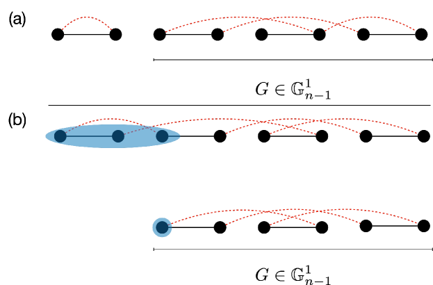
Figure S1: Visualization of the inductive step in the proof of the first moment of the output probabilities (Theorem 1 in the main text, restated here in the SM as Theorem S1). The inductive step proceeds in two cases that are determined by the red edge that connects to the first vertex in the graph in $\mathbb{G}_{n}^{1}$. In (a), we consider the case where the first two vertices, which are linked by a black (solid) edge, are also linked by a red (dashed) edge, meaning they comprise a single connected component. This contributes a factor of $k$ times the contribution from a graph in $\mathbb{G}_{n-1}^{1}$, which comes from the remaining $2n-2$ vertices and their edges. (b) considers the case where the first vertex is linked via a red edge to a different vertex $O_{a}\neq O_{2}$ for which there are $2n-2$ choices (here $a=3$). The number of connected components does not change after identifying and combining the three vertices that are connected in this way (visualized by the blue background), meaning we again reduce down to a graph in $\mathbb{G}_{n-1}^{1}$, but this time without the multiplicative factor of $k$.

Overall then, we find that

$$f(k,n) =kf(k,n-1)+(2n-2)f(k,n-1)$$ (S32)

$$=(k+2n-2)f(k,n-1)$$ (S33)

$$=(k+2n-2)(k+2n-4)\dots(k+2)k,$$ (S34)

which proves the formula (and where the inductive hypothesis is used in the final equality). ∎

We note briefly that the structure of this proof is similar to that used in Ref. Arrazola et al. (2018) to calculate $\underset{X\sim\mathcal{G}^{n\times n}}{\operatorname*{\mathbb{E}}}[\absolutevalue{\mathrm{Haf}{X}}^{4}]$. The proofs are similar because there are four copies of $X$ in each, but the proofs are not identical given that different definitions of the hafnian are used. Additionally, similar graphs, and a similar calculation involving enumerating the number of graphs of a given number of connected components, show up in the bioinformatic study of breakpoint graphs (which are a type of graph defined by two perfect matchings that show up in the theory of comparative genomics) Feijão et al. (2015).

We next move on to a proof of Theorem 2, which gives the form of the second moment as a polynomial in $k$. We again restate the theorem for convenience.

Theorem S2.

The second moment $M_{2}(k,n)$ is a degree-$2n$ polynomial in $k$ and can be written as $M_{2}(k,n)=(2n-1)!!\sum_{i=1}^{2n}c_{i}k^{i}$, where $c_{i}$ is the number of graphs $G\in\mathbb{G}^{2}_{n}$ that have $i$ connected components.

Proof.

As mentioned in the main text, once Eq. 9 is derived, the theorem follows after deriving the correct limits of summation. Trivially, the fewest possible number of connected components is $1$. To see that the largest possible number of connected components is $2n$, we consider the four patterns of black edges that are illustrated in Fig. 2(b) of the main text and how many connected components can possibly occur in graphs with those different patterns. See also Fig. S2 for a reminder of the patterns of black edges and a visual explanation of the following argument.

First note that, because all vertices are paired via black edges, every connected component has an even number of vertices. Therefore, the two smallest sizes of connected components are $2$ and $4$ vertices. In order to get a connected component of size $2$, one must connect a pair of vertices with both a black and a red edge. Red edges are constrained to lie in a single row, meaning only type-1 and type-4 patterns of black edges, which contain a pair of vertices connected by a black edge in the same row, can yield a connect component of size $2$. Pairing off the remaining vertical black edges yields connected components of size $4$, the next smallest size.

Therefore, the maximum number of connected components arises from taking only type-1 and type-4 edges. This requires connecting each horizontal black edge by red edge (creating a connected component with $2$ vertices) and then pairing off the vertical edges coming from the same type. This allows for the maximal $2$ connected components per set of six vertices, meaning $2n$ total connected components. ∎

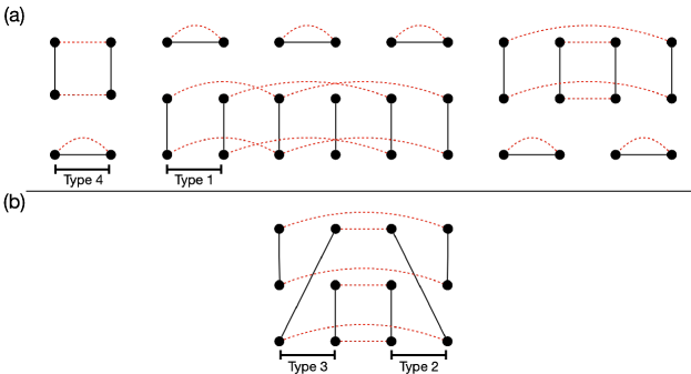
Figure S2: (a) Example graph in $\mathbb{G}_{6}^{2}$ showing how to achieve an average of two connected components per set of six vertices using only type-1 and type-4 sets of edges. All vertices connected by horizontal black (solid) edges are also connected by red (dashed) edges. All type-1 vertical edges are paired off, as are type-4 vertical edges. Note that this graph would correspond to $z=1+3\times 4^{0}+0\times 4^{1}+0\times 4^{2}+0\times 4^{3}+3\times 4^{4}+3\times 4^{5}=3844$. (b) Example showing how using type-2 and type-3 black edges lead to, at most, three connected components per two sets of six vertices.

We also prove Lemma 1, which we again restate for convenience:

Lemma S1.

We have that

1. $M_{2}(1,n)=((2n-1)!!)^{4}4^{n}$

2. $c_{2n}=(2n)!!$

Proof.

Part (i): examine Eq. S24. Because $k=1$, $o_{i}=p_{i}=q_{i}=1$ for all $i$. Thus, regardless of the permutation, all Kronecker $\delta$s are always satisfied. This means that, independent of the permutation, each factor is always $4$ such that the product becomes $4^{n}$. The sum over the three copies of $S_{2n}$ then simply yields a factor of $(2n)!^{3}$. The result then follows.

Part (ii): we argued in the proof of Theorem S2 that the leading-order term in the polynomial expansion of the second moment is $k^{2n}$, and it comes from graphs that consist of only type-1 and type-4 black edges. Each type-1 and type-4 set of edges contains a horizontal black edge, and the two vertices linked by that black edge also must be linked by a red edge to create a $2$-vertex connected component. Additionally, the vertical edges of the type-1 sets need to be paired off via red edges; similarly, the vertical edges of the type-4 sets need to be paired off. This ensures that each other connected component has exactly $4$ vertices, maximizing the number of possible connected components.

Fig. S3 visualizes how to now reduce the remaining calculation to the value of the first moment when $k=2$. If we imagine collapsing each pair of adjacent vertical edges (i.e., those coming from the same group of $6$ vertices) onto a pair of vertices connected by a black edge, we reproduce the atomic graph from the proof of the first moment. Here, by atomic graph, we mean the vertices and the fixed black edges which are shared by all graphs; the red edges are not yet included. Explicitly, there are $2n$ vertices, and vertices $O_{2i-1},O_{2i}$ are connected with a black edge. The black edges here act to identify that the original uncollapsed vertical edges were of the same type. Drawing red edges in the simplified graph on $2n$ vertices corresponds to pairing off vertical edges in the original graph on $6n$ vertices with red edges. Note that this also implies that red edges connect vertical edges of the same type. Therefore, a connected component in the simplified graph could correspond to two preimages in the original graph: either all type-1 vertical edges, or all type-4 vertical edges. Then, by summing over all graphs and weighting each connected component by $2$, we are effectively evaluating $f(2,n)$ in Eq. S31, i.e.:

$$f(2,n)=\frac{(k+2n-2)!!}{(k-2)!!}\bigg{|}_{k=2}=(2n)!!.$$ (S35)

∎

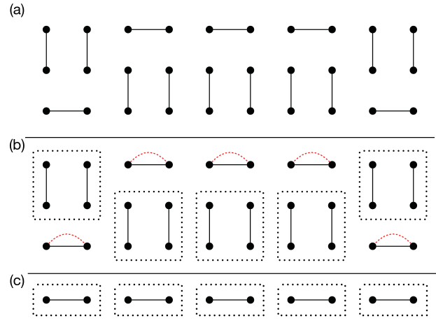
Figure S3: Visualization of how the calculation of the coefficient of the leading-order term in the second moment can be reduced to the $k=2$ case of the first moment. Recall that black edges are solid and red edges are dashed. (a) As proven in Theorem 2, graphs that maximize the number of connected components contain only type-1 and type-4 black edges. (b) To maximize the number of connected components, the horizontal black edges must form their own connected component with two vertices, meaning their vertices must be connected by a red edge. Furthermore, each vertical black edge must be paired off with exactly one other vertical black edge of the same type, forming a connected component with $4$ vertices. We draw dotted boxes around the two black vertical edges to show that they come from the same type. (c) If we collapse each vertical edge onto a single vertex and then connect that vertex to the vertex stemming from its adjacent edge in the original graph (i.e. the other vertical edge from the same group of six vertices), then we reduce to the atomic graph (i.e., the graph with the fixed black edges, but without red edges) from the proof of the first moment. Red edges on this collapsed graph would then correspond to pairing off vertical edges in the original graph with red edges. Because paired edges in the original graph can only exist between edges of the same type, each connected component in the simplified graph could have come from either type-1 or type-4 vertical edges. This is equivalent to setting $k$, the contribution from each connected component, to $2$, and then evaluating $f(2,n)$.

S4 Details on Definitions of Anticoncentration

In this section, we discuss in somewhat more detail the relevance of anticoncentration to the argument for hardness of sampling from the output distribution of Gaussian Boson Sampling (GBS). This argument makes use of an approximate counting algorithm due to Stockmeyer (1983). Roughly, we assume that there is an efficient sampling algorithm for GBS that, given a linear-optical unitary $U$, samples from a distribution $Q_{U}$ which is close up to a constant $\epsilon>0$ to the ideal GBS distribution $P_{U}$ (recall Eq. 1 of the main text) in total-variation distance

$$\mathsf{tvd}(P_{U},Q_{U})\coloneqq\frac{1}{2}\sum_{\mathbf{n}}|P_{U}(\mathbf{n})-Q_{U}(\mathbf{n})|\leq\epsilon.$$ (S36)

Supposing such a sampling algorithm exists, and given the so-called hiding property (see Sec. D of Ref. Hangleiter and Eisert (2023) for details), we can use it as input to Stockmeyer’s algorithm. Stockmeyer’s algorithm then approximates the probability $P_{U}(\mathbf{n})$ up to an error given by

$$\varepsilon=\frac{1}{\mathrm{poly}(n)}P_{U}(\mathbf{n})+\frac{2\epsilon}{|\Omega|\delta}\left(1+\frac{1}{\mathrm{poly}(n)}\right),$$ (S37)

with probability $1-\delta$ over $\mathbf{n}$, where $\Omega$ is the effective sample space on which $P_{U}$ is defined. If it is sufficiently hard (#P-hard, to be precise) to approximate the outcome probabilities $P_{U}(\mathbf{n})$ up to the error (S37), on the instances on which our approximation scheme achieves this error, this rules out the approximate sampling algorithm up to very reasonable complexity-theoretic conjectures (one of which is the non-collapse of the polynomial hierarchy, a generalization of the famous P $\neq$ NP conjecture). The required property is thus what we call “approximate average-case hardness,” that is, the statement that any algorithm which is able to compute $P_{U}(\mathbf{n})$ with probability $1-\delta$ over the instances up to the error (S37) is able to solve any #P-hard problem (of the same difficulty as approximating the outcome probabilities $P_{U}(\mathbf{n})$ up to the error (S37)).

While we know average case hardness of approximating the outcome probabilities up to error $2^{-\Omega(n\log n)}$ Bouland et al. (2022); Deshpande et al. (2022a), it is only conjectured for the relevant approximation error given by either $c_{1}P_{U}(\mathbf{n})$ or $c_{2}/|\Omega|$ for constants $c_{1},c_{2}>0$. Anticoncentration serves as evidence for the truth of the conjecture, the idea being the following: suppose that most of the outcome probabilities are very close to zero, i.e. $\ll\epsilon/2^{-n}$, meaning only a vanishing fraction of them are relevant. Then a high approximation error on the relevant probabilities is tolerable, because we only need to distinguish between relevant and irrelevant outcomes, and a sufficiently good approximation to the irrelevant ones is zero. This is a significantly easier task than if the distribution is highly spread out and a large fraction of the probabilities is “relevant” in the sense that all of the relevant probabilities are of the same order of magnitude as the uniform distribution.

In the standard argument, this intuition is formalized as the statement

$$\Pr_{U\in\mathrm{U}(m)}\left[P_{U}(\mathbf{n})\geq\frac{\alpha}{|\Omega|}\right]\geq\gamma(\alpha),$$ (S38)

for some constants $\alpha,\gamma(\alpha)>0$. In this formulation, we have made crucial use of the hiding property, which asserts that the distribution over circuits is invariant under a procedure by which we “hide” a particular outcome $\mathbf{n}$ in the probability of obtaining a different outcome $\mathbf{n}^{\prime}$ of a random circuit. This allows us to restrict our attention to the distribution over circuits of a fixed outcome $\mathbf{n}$.

The anticoncentration property (S38) implies that the error (S37) is dominated by the first term on a $\gamma(\alpha)(1-\delta)$ fraction of the instances because with probability $\gamma(\alpha)$ we can upper bound the second term by $P_{U}(\mathbf{n})$. But, if a large fraction of the probabilities is larger than uniform, then none of them can be much larger than uniform and, hence, the approximation error needs to be exponentially small. Thus, we expect that, in the presence of anticoncentration, approximating the outcome probabilities up to the error (S37) is much harder than without anticoncentration, lending credibility to the approximate average-case hardness conjecture.

In our definition of anticoncentration, we consider the (normalized) average collision probability

$$P_{2}(\mathrm{U}(m))\coloneqq|\Omega|\sum_{\mathbf{n}\in\Omega}\operatorname*{\mathbb{E}}_{U\in\mathrm{U}(m)}\left[P_{U}(\mathbf{n})^{2}\right]$$ (S39)

$$\stackrel{{\scriptstyle\text{hiding}}}{{=}}|\Omega|^{2}\operatorname*{\mathbb{E}}_{U\in\mathrm{U}(m)}\left[P_{U}(\mathbf{n})^{2}\right].$$ (S40)

The collision probability is the probability that, were one to sample the distribution twice, one would receive the same outcome both times. For very flat distributions it is very small. With the normalization, the collision probability of the uniform distribution is given by $1$, which is its minimal value. On the other hand, the normalized collision probability of a fully peaked distribution with a single unit probability is given by $|\Omega|$.

The average collision probability is thus another measure of the anticoncentration of the outcome probabilities in the ensemble of linear-optical unitaries. It is a more coarse-grained measure, though, because it is only an average quantity. Indeed, a (constantly) small average collision probability implies anticoncentration in the sense of (S38) via the Paley-Zygmund inequality as

$$\Pr_{U\in\mathrm{U}(m)}\left[P_{U}(\mathbf{n})\geq\frac{\alpha}{|\Omega|}\right]\geq(1-\alpha)^{2}\frac{1}{P_{2}(\mathrm{U}(m))}.$$ (S41)

The relevant quantity of interest to anticoncentration is thus the inverse average collision probability $p_{2}(\mathrm{U}(m))=1/P_{2}(\mathrm{U}(m)$. Because by hiding the first moment $\operatorname*{\mathbb{E}}_{U}[P_{U}(\mathbf{n})]$ must evaluate to the inverse size of the effective sample space, we can rewrite $p_{2}$ for GBS as

$$p_{2}(\mathrm{U}(m))=\frac{\operatorname*{\mathbb{E}}_{U\in\mathrm{U}(m)}[P_{U}(\mathbf{n})]^{2}}{\operatorname*{\mathbb{E}}_{U\in\mathrm{U}(m)}[P_{U}(\mathbf{n})^{2}]}\approx\frac{M_{1}(k,n)^{2}}{M_{2}(k,n)}=m_{2}(k,n).$$ (S42)

In the main text, we define various degrees of anticoncentration in terms of the inverse average collision probability $p_{2}$, which we recall here.

• We say that $P_{U},U\in\mathrm{U}(m)$ anticoncentrates if $p_{2}=\Omega(1)$.

• We say that $P_{U}$ anticoncentrates weakly if $p_{2}=\Omega(1/n^{a})$ for some $a=O(1)$.

• And we say that it does not anticoncentrate if $p_{2}=O(1/\exp(n))$.

Here, we motivate those definitions in more detail. Clearly (A) implies anticoncentration in the sense of Eq. S38, hence the definition.

Lack of anticoncentration (NA)

Ignoring the average over unitaries, $p_{2}$ upper-bounds the support of the distribution by $p_{2}|\Omega|$, as the maximum-entropy state is the uniform distribution. Hence, an exponentially small value of $p_{2}$ implies that the average support of the outcome distributions $P_{U}$ is exponentially small, implying that at least a constant fraction (over $U$) of the distributions $P_{U}$ has exponentially small support, and conversely exponentially larger than uniform probabilities on that support. At least for those distributions, this implies an exponentially larger error tolerance compared to $1/|\Omega|$. Such an exponentially larger error tolerance makes the approximate average-case hardness conjecture significantly stronger, presumably even untenable.

While it is possible that for a constant fraction of the $U$ we are in this scenario (see Sec. V.C of Ref. Deshpande et al. (2022b) for an example), while for another constant fraction, the probabilities are highly spread out, making the anticoncentration property (S38) true, this seems like an extremely unlikely state of affairs. Indeed, the hiding property implies that it should not matter whether we talk about the distribution over unitaries or over outcomes, which means that the situation described above is a generic feature, rendering (S38) false in case $p_{2}$ is exponentially small.

Weak anticoncentration (WA)

Our results show that weak anticoncentration holds in the regime of $k\rightarrow\infty$. But why do we think of a polynomially decaying $p_{2}$ as weak anticoncentration rather than no anticoncentration?

We argue that this is a meaningful regime in the sense that there is a stronger—but not inconceivable—approximate average-case hardness conjecture associated with the weak anticoncentration regime. To see this, observe that weak anticoncentration implies anticoncentration in the sense of Eq. S38 with $\gamma(\alpha)=\Omega(1/\textrm{poly}(n))$, which means that an inverse polynomial fraction of the outcome probabilities are larger than uniform. Technically, using Stockmeyer’s algorithm we can thus achieve a multiplicative error for an inverse polynomial fraction of the outcome probabilities. To rule out an efficient classical sampler, we thus need to conjecture approximate average-case hardness with constant relative errors for any inverse polynomial fraction of the instances. Equivalently, we can formulate a similar conjecture for a polynomially large relative or subexponentially large additive error on a constant fraction. While clearly much stronger than the requirement of anticoncentration, this is qualitatively different from the lack of anticoncentration scenario (NA), where the difference is exponential.

S5 Scattershot Boson Sampling Explanation of the Transition in Anticoncentration

In Scattershot Boson Sampling (SBS), the setup is as follows. $m=\omega(n^{2})$ two-mode squeezed states with squeezing parameter $r$ are prepared. The photon number distribution of the two-mode squeezed states is supported on Fock states of the form $\ket{n}\ket{n}$ for $n\in\mathbb{N}_{0}$. One half of each two-mode squeezed state is then measured in the Fock basis, yielding, with high probability, an outcome $n_{i}\in\{0,1\}$ (assuming $r$ is small enough). Collecting outcomes in the vector $\mathbf{n}=(n_{1},\ldots,n_{m})$, the other half of the input modes is now in the postselected state $\ket{\mathbf{n}}=\bigotimes_{i=1}^{m}\ket{n_{i}}$. The outcome probabilities after passing this input state through the linear optical unitary $U$ and measuring in the Fock basis yielding outcome $\mathbf{o}=(o_{1},\ldots,o_{m})$, $o_{i}\in\{0,1\}$ is then given by

$$P_{U}(\mathbf{n},\mathbf{o})=|\mathrm{Per}(U_{\mathbf{n},\mathbf{o}})|^{2}$$ (S43)

of the submatrix $U_{\mathbf{n},\mathbf{o}}$ in which we select the rows and columns according to the indices with nonzero entries in $\mathbf{n}$ and $\mathbf{o}$. But conditioned on input and output states being collision-free and the hiding property, the distribution of matrices $U_{\mathbf{n},\mathbf{o}}$ equals that of the Boson Sampling submatrices $U_{\mathbf{1}_{n},\mathbf{o}}$, where the photons in the input state are by convention in the first $n$ modes. The properties of Scattershot Boson Sampling postselected on collision-free outcomes in a fixed photon number sector are therefore equal to the properties of standard Boson Sampling.

We now argue that this equivalency hinges essentially on the fact that at least $\omega(n^{2})$ of the input modes are squeezed. To this end, consider a modification of Scattershot Boson Sampling in which only $k$ out of the $m$ modes are prepared in one half of a two-mode squeezed state, while the remaining $m-k$ modes are prepared in the vacuum state. This closely resembles the GBS setting, of course. Let us also consider a squeezing parameter $r$ of every two-mode squeezed state chosen such that the mean photon number after postselection is given by $n$. To achieve this, we pick the mean photon number per mode, which is given by $\sinh^{2}(r)$ to be equal $n/k$ to obtain a total of $k\sinh^{2}r=n$ photons on average. This ensures that in the postselection we end up with $n$ photons with high probability.

Let us for simplicity assume that the photon numbers observed in the postselection measurement are Poissonian distributed as $p(l)=\sinh^{2l}(r)\mathrm{e}^{-\sinh^{2}(r)}/l!$ with mean $\sinh^{2}(r)=n/k$. Then the probability of observing a collision scales as

$$\Pr[\text{collision}]=1-\left(\left(1+\frac{n}{k}\right)e^{-n/k}\right)^{k}=1-\exp\left(-\frac{n^{2}}{2k}+\sum_{l=3}^{\infty}\frac{(-1)^{l+1}}{l}\frac{n^{l}}{k^{l-1}}\right),$$ (S44)

assuming $k=\omega(n)$. This collision probability remains lower bounded by a constant for $k=O(n^{2})$, but vanishes for any $k=\omega(n^{2})$. Thus, the probability of a collision in the input state of SBS remains high until $k=\Theta(n^{2})$ and decays then. But because in SBS the roles of the (postselected) input state and the output state are symmetric, a collision implies a failure of hiding and therefore a failure of anticoncentration in the regime $k=O(n^{2})$. Conversely, for $k=\omega(n^{2})$ we believe that hiding holds Jiang (2006); Aaronson and Arkhipov (2013), and hence Lemma 8.8 of Aaronson and Arkhipov (2013) shows weak anticoncentration for SBS with the inverse average collision probability $p_{2}=1/n$ in this regime.

This shows that generalized SBS with a variable number of input squeezed states undergoes a transition in anticoncentration as we find it here for the case of GBS. It is not at all clear that the transition in SBS implies a transition in GBS, however, as GBS does not involve postselection. Indeed, in SBS, the anticoncentration coincides with—or rather is—a transition in the hiding property. In GBS, in contrast, hiding is conjectured to hold for all $k$, while we do see the transition in anticoncentration. The situation in GBS is not immediately comparable to that in this modified SBS scenario because the input single-mode squeezed states are supported on even numbers of photons, and therefore any nonzero photon number input states are collision-full. Therefore, as mentioned in the discussion in the main text, the possible connections outlined here deserve future consideration.