New High-Order Numerical Methods for Hyperbolic Systems of Nonlinear PDEs with Uncertainties

Abstract

In this paper, we develop new high-order numerical methods for hyperbolic systems of nonlinear partial differential equations (PDEs) with uncertainties. The new approach is realized in the semi-discrete finite-volume framework and it is based on fifth-order weighted essentially non-oscillatory (WENO) interpolations in (multidimensional) random space combined with second-order piecewise linear reconstruction in physical space. Compared with spectral approximations in the random space, the presented methods are essentially non-oscillatory as they do not suffer from the Gibbs phenomenon while still achieving a high-order accuracy. The new methods are tested on a number of numerical examples for both the Euler equations of gas dynamics and the Saint-Venant system of shallow-water equations. In the latter case, the methods are also proven to be well-balanced and positivity-preserving.

Keywords: Hyperbolic conservation and balance laws with uncertainties, finite-volume methods, central-upwind schemes, weighted essentially non-oscillatory (WENO) interpolations.

AMS subject classification: 65M08, 76M12, 35L65, 35R60.

1 Introduction

Many important scientific problems contain sources of uncertainties in parameters, initial and boundary conditions (ICs and BCs), etc. In partial differential equations (PDEs), uncertainties may be described with the help of random variables. In this paper, the focus is placed on hyperbolic systems of conservation and balance laws with uncertainties. Such systems read as

$$\bm{U}_{t}+\nabla_{\bm{x}}\cdot\bm{F}=\bm{S},$$ (1.1)

where $\bm{U}(\bm{x},t,\bm{\xi})\in\mathbb{R}^{N}$ is an unknown vector-function, $\bm{F}(\bm{U}):\mathbb{R}^{N}\to\mathbb{R}^{N}$ are the flux functions, and $\bm{S}(\bm{U},\bm{x},\bm{\xi})$ is a source term. Furthermore, $t$ is time and $\bm{x}\in\mathbb{R}^{d}$ are spatial variables. Without loss of generality we assume that $\bm{\xi}\in\Xi\subset\mathbb{R}^{s}$ are real-valued random variables. We denote by $(\Xi,{\cal F},\nu)$ the underlying probability space, where $\Xi$ is a set of events, ${\cal F}(\Xi)$ is the $\sigma$-algebra of Borel measurable sets, and $\nu(\bm{\xi}):\Xi\to\mathbb{R}_{+}$ is the probability density function, $\nu\in L^{1}(\Xi)$.

The system (1.1) arises in many applications, including fluid dynamics, geophysics, electromagnetism, meteorology, and astrophysics, to name a few. Quantifying uncertainties that appear as input quantities, as well as in the ICs and BCs due to empirical approximations or measuring errors, is essential as it helps to perform sensitivity analysis and provides guidance to improve models.

We are interested in developing highly accurate and robust numerical methods for (1.1). Several methods have already been developed. Monte Carlo-type methods (see, e.g., [2, 35, 34, 33, 31, 32]) are reliable but not computationally efficient due to the large number of realizations required to achieve accurate approximation of statistical moments. Another widely used approach for solving (1.1) is the generalized polynomial chaos (gPC), where the solution is sought in terms of a series of orthogonal polynomials with respect to the probability density in $\bm{\xi}$; see, e.g., [26, 38, 55, 56]. There are two types of gPC methods: intrusive and non-intrusive ones. In non-intrusive algorithms, such as stochastic collocation (gPC-SC) methods, one seeks to satisfy the governing equations at a discrete set of nodes in the random space, employing the same numerical solver as for the deterministic problem and then using interpolation and quadrature rules to evaluate statistical moments numerically; see, e.g., [55, 43, 54, 56, 38, 45]. In intrusive approaches, such as stochastic Galerkin (gPC-SG) methods, the gPC expansions are substituted into the governing equations and projected by a Galerkin approximation to obtain deterministic equations for the expansion coefficients; see, e.g., [47, 48, 9, 13, 7, 8, 16, 15, 17, 22, 38, 39, 41, 52, 53, 57]. Solving the coefficient equations yields the statistical moments of the original uncertain problem solution.

Several challenges are associated with applying the gPC-SC and gPC-SG methods to nonlinear hyperbolic systems (1.1). It is well-known that spectral-type gPC-based methods exhibit fast convergence when the solution depends smoothly on the random parameters. However, one of the main problems in using these methods is related to the lack of smoothness of their solutions, which may break down in finite time as a result of the development of shock and contact waves. Although these discontinuities appear in spatial variables, their propagation speed can be affected by uncertainty, causing discontinuities in random variables and triggering aliasing errors [6] and Gibbs-type phenomena [27] (see also [49, 20, 1, 4]). Another open question in gPC-based stochastic methods is the representation of strictly positive quantities such as gas density or water depth and/or the enforcement of discrete bound-preserving constraints; see, e.g., [7, 8, 17, 26, 39]. It can also be shown that gPC-based methods, which are highly accurate for moment estimation, might fail to approximate the probability density function, even for the one-dimensional (1-D) noise [10]. An additional numerical difficulty associated with implementing the gPC-SG methods is posed by the fact that the deterministic Jacobian of the projected system differs from the random Jacobian of the original system. Therefore, when applied to general nonlinear hyperbolic systems, the gPC-SG method results in a system for expansion coefficients, which is not necessarily globally hyperbolic [9]. Consequently, additional effort is needed to develop stable numerical methods for (potentially ill-posed) systems for the gPC coefficients; see, e.g., [13, 26, 40, 39, 38, 48, 7, 8, 16, 15, 17, 41, 52, 53].

In this paper, we propose a new approach in which we conduct the approximation in the random space using weighted essentially non-oscillatory (WENO) interpolants rather than orthogonal polynomial expansions, which are highly oscillatory in the case of nonsmooth solutions. The new approach is realized in the semi-discrete finite-volume framework. The system (1.1) is integrated over the $(\bm{x},\bm{\xi})$-cells and the solution is obtained in terms of cell averages, which are evolved in time using numerical fluxes in the $\bm{x}$-directions. These fluxes are evaluated with the help of a second-order piecewise linear reconstruction in $\bm{x}$ and a Gauss-Legendre quadrature in $\bm{\xi}$ is implemented using high-order WENO interpolants. This allows one to achieve high accuracy in $\bm{\xi}$ even in the generic case of discontinuous solutions. We refer the reader to related work in [2, 3, 14, 37, 46], where a similar idea has been used in the framework of stochastic finite-volume methods. In this work, we implement a second-order finite-volume method in physical space. It is combined with a high-order WENO interpolation in the random space. Notice that by using a high-order WENO interpolation, we not only keep a high-order approximation in the random space but also properly (without the Gibbs phenomenon) resolve discontinuities that may propagate into the random directions.

The new family of methods may use different numerical fluxes, piecewise-linear reconstructions, and high-order interpolations. A particular choice made in this work is the following. We use the Riemann-problem-solver-free central-upwind (CU) fluxes introduced in [23, 24]; the generalized minmod reconstruction in $\bm{x}$ (see, e.g., [29, 36, 44]); the fifth-order Gauss-Legendre quadrature (for uniformly distributed random variables); and the recently proposed fifth-order affine-invariant WENO-Z (Ai-WENO-Z) interpolation in $\bm{\xi}$ (see [12, 28, 50]), which is a stabilized version of the original WENO-Z interpolation (see, e.g., [11, 21, 30, 51]). It should be observed that the lack of boundary conditions in the random space impose an additional difficulty as it requires the development of a special high-order interpolation technique near the boundary. In this paper, we overcome this difficulty by designing a new one-sided Ai-WENO-Z interpolation. In addition, we restrict our consideration to the simplest 1-D case ($d=s=1$) and two higher-dimensional extensions ($d=1$, $s=2$ and $d=2$, $s=1$), all with uniformly distributed random variables, while providing ideas how the proposed methods can be extended to different random distributions. We test the resulting scheme on several numerical examples for both the Euler equations of gas dynamics and the Saint-Venant system of shallow water equations. For the latter application, we use the same technique as in [24] to enforce the well-balanced (WB) property, that is, to make the scheme capable of exactly preserving “lake-at-rest”/still-water steady-state solutions.

2 One-Dimensional Semi-Discrete Scheme

In the 1-D case ($d=s=1$), the system (1.1) reduces to

$$\bm{U}_{t}+\bm{F}(\bm{U})_{x}=\bm{S}(\bm{U},x,\xi),$$ (2.1)

which we discretize on a finite-volume mesh with cells $C_{j,\ell}=[x_{j-\frac{1}{2}},x_{j+\frac{1}{2}}]\times[\xi_{\ell-\frac{1}{2}},\xi_{\ell+\frac{1}{2}}]$, $j=1,\ldots,N_{x}$, $\ell=1,\ldots,N_{\xi}$, taken to be uniform both in $x$ and $\xi$. Here, $x_{j+\frac{1}{2}}-x_{j-\frac{1}{2}}\equiv\Delta x$ and $\xi_{\ell+\frac{1}{2}}-\xi_{\ell-\frac{1}{2}}\equiv\Delta\xi$, and the cells are centered at $(x_{j},\xi_{\ell})=\Big{(}\frac{x_{j-\frac{1}{2}}+x_{j+\frac{1}{2}}}{2},\frac{\xi_{\ell-\frac{1}{2}}+\xi_{\ell+\frac{1}{2}}}{2}\Big{)}$.

The computed cell averages are assumed to be available at a certain time $t$:

$$\hbox{\vbox{\hrule height=0.5pt\kern 1.72218pt\hbox{\kern-0.50003pt$\bm{U}$\kern 0.0pt}}}_{j,\ell}(t)\approx\frac{1}{\Delta x\Delta\xi}\iint\limits_{C_{j,\ell}}\bm{U}(x,\xi,t)\,\nu(\xi)\,{\rm d}x\,{\rm d}\xi.$$

These quantities are evolved in time using a semi-discretization of (2.1):

$$\frac{\rm d}{{\rm d}t}\,\hbox{\vbox{\hrule height=0.5pt\kern 1.72218pt\hbox{\kern-0.50003pt$\bm{U}$\kern 0.0pt}}}_{j,\ell}(t)=-\frac{\bm{{\cal F}}_{{j+\frac{1}{2}},\ell}(t)-\bm{{\cal F}}_{{j-\frac{1}{2}},\ell}(t)}{\Delta x}+\hbox{\vbox{\hrule height=0.5pt\kern 1.72218pt\hbox{\kern-0.50003pt$\bm{S}$\kern 0.0pt}}}_{j,\ell}(t),$$ (2.2)

where $\bm{{\cal F}}_{{j+\frac{1}{2}},\ell}$ are numerical fluxes (see §2.1) and $\hbox{\vbox{\hrule height=0.5pt\kern 1.72218pt\hbox{\kern-0.50003pt$\bm{S}$\kern 0.0pt}}}_{j,\ell}$ are approximated cell averages of the source term:

$$\hbox{\vbox{\hrule height=0.5pt\kern 1.72218pt\hbox{\kern-0.50003pt$\bm{S}$\kern 0.0pt}}}_{j,\ell}(t)\approx\frac{1}{\Delta x\Delta\xi}\iint\limits_{C_{j,\ell}}\bm{S}(\bm{U},x,\xi)\,\nu(\xi)\,{\rm d}x\,{\rm d}\xi.$$ (2.3)

Note that all indexed quantities that depend on $\bm{U}$ are time-dependent, but from now on, this dependence will be omitted for the sake of brevity.

2.1 Numerical Fluxes and Source Terms

The numerical fluxes in (2.2) are obtained by averaging the fluxes in the $\xi$-direction:

$$\bm{{\cal F}}_{{j+\frac{1}{2}},\ell}=\sum_{i=1}^{M}\mu_{i}\,\nu(\xi_{\ell_{i}})\,\bm{{\cal F}}\big{(}\bm{U}^{-}_{{j+\frac{1}{2}},\ell_{i}},\bm{U}^{+}_{{j+\frac{1}{2}},\ell_{i}}\big{)},$$ (2.4)

where the integration in the $\xi$-direction has been performed using a Gauss-Legendre quadrature on the cell $[\xi_{\ell-\frac{1}{2}},\xi_{\ell+\frac{1}{2}}]$ with the weights $\mu_{i}$ and nodes $\xi_{\ell_{i}}\in(\xi_{\ell-\frac{1}{2}},\xi_{\ell+\frac{1}{2}})$, $i=1,\ldots,M$. Furthermore, $\bm{{\cal F}}$ is computed using the reconstructed one-sided point values of $\bm{U}$ at $(x_{j+\frac{1}{2}}\pm 0,\xi_{\ell_{i}})$, which are denoted by $\bm{U}^{\pm}_{{j+\frac{1}{2}},\ell_{i}}$. We use the CU numerical flux from [23]:

$$\bm{{\cal F}}\big{(}\bm{U}^{-}_{{j+\frac{1}{2}},\ell_{i}},\bm{U}^{+}_{{j+\frac{1}{2}},\ell_{i}}\big{)} =\frac{a_{{j+\frac{1}{2}},\ell}^{+}\bm{F}\big{(}\bm{U}^{-}_{{j+\frac{1}{2}},\ell_{i}}\big{)}-a_{{j+\frac{1}{2}},\ell}^{-}\bm{F}\big{(}\bm{U}^{+}_{{j+\frac{1}{2}},\ell_{i}}\big{)}}{a_{{j+\frac{1}{2}},\ell}^{+}-a_{{j+\frac{1}{2}},\ell}^{-}}$$ (2.5)

$$+\frac{a_{{j+\frac{1}{2}},\ell}^{+}a_{{j+\frac{1}{2}},\ell}^{-}}{a_{{j+\frac{1}{2}},\ell}^{+}-a_{{j+\frac{1}{2}},\ell}^{-}}\left(\bm{U}^{+}_{{j+\frac{1}{2}},\ell_{i}}-\bm{U}^{-}_{{j+\frac{1}{2}},\ell_{i}}\right),$$

where $a_{{j+\frac{1}{2}},\ell}^{\pm}$ are the one-sided local speeds of propagation in the $x$-direction at $(x_{j+\frac{1}{2}},\xi_{\ell})$, which can be estimated using the smallest ($\lambda_{1}$) and largest ($\lambda_{N}$) eigenvalues of the Jacobian $\frac{\partial\bm{F}}{\partial\bm{U}}$:

$$a_{{j+\frac{1}{2}},\ell}^{-}=\min\left\{\lambda_{1}\left(\frac{\partial\bm{F}}{\partial\bm{U}}\left(\bm{U}^{-}_{{j+\frac{1}{2}},\ell}\right)\right),\,\lambda_{1}\left(\frac{\partial\bm{F}}{\partial\bm{U}}\left(\bm{U}^{+}_{{j+\frac{1}{2}},\ell}\right)\right),\,0\right\},$$ (2.6)

$$a_{{j+\frac{1}{2}},\ell}^{+}=\max\left\{\lambda_{N}\left(\frac{\partial\bm{F}}{\partial\bm{U}}\left(\bm{U}^{-}_{{j+\frac{1}{2}},\ell}\right)\right),\,\lambda_{N}\left(\frac{\partial\bm{F}}{\partial\bm{U}}\left(\bm{U}^{+}_{{j+\frac{1}{2}},\ell}\right)\right),\,0\right\}.$$

Finally, the integral on the right-hand side (RHS) of (2.3) is discretized in two steps. First, we use the same Gauss-Legendre quadrature as in (2.4) to numerically integrate with respect to $\xi$ and obtain

$$\hbox{\vbox{\hrule height=0.5pt\kern 1.72218pt\hbox{\kern-0.50003pt$\bm{S}$\kern 0.0pt}}}_{j,\ell}=\frac{1}{\Delta x}\sum_{i=1}^{M}\mu_{i}\,\nu(\xi_{\ell_{i}})\int\limits_{x_{j-\frac{1}{2}}}^{x_{j+\frac{1}{2}}}\bm{S}(\bm{U}(x,\xi_{\ell_{i}},t),x,\xi_{\ell_{i}})\,{\rm d}x.$$ (2.7)

Second, depending on the system at hand, we choose a proper quadrature for the integrals on the RHS of (2.7). In the case of the Saint-Venant system considered in §6, a special quadrature for the geometric source term will be introduced to enforce a WB property of the resulting scheme.

2.2 Reconstruction of the Point Values

This section describes the reconstruction procedures in both physical and random space. We use a piecewise linear reconstruction in $x$ and a high-order reconstruction in $\xi$. The order of the resulting scheme in $\xi$ depends on the accuracy of the quadratures used to evaluate the numerical flux and source terms in (2.4) and (2.7). In this paper, we use the fifth-order Gauss-Legendre quadrature with $M=3$ and the corresponding weights

$$\mu_{1}=\mu_{3}=\frac{5}{18},\quad\mu_{2}=\frac{4}{9},$$ (2.8)

and nodes $\xi_{\ell_{i}}$, $i=1,2,3$ with

$$\xi_{\ell_{1}}=\xi_{\ell-\kappa},\quad\xi_{\ell_{2}}=\xi_{\ell},\quad\xi_{\ell_{3}}=\xi_{\ell+\kappa},\quad\kappa=\sqrt{\frac{3}{5}}.$$ (2.9)

We will therefore first apply a picewise linear reconstruction in the $x$-direction to obtain the one-sided point values $\bm{U}_{{j+\frac{1}{2}},\ell}^{\pm}$ at the midpoints of the cell interfaces $(x_{j+\frac{1}{2}},\xi)$, $\xi\in(\xi_{\ell-\frac{1}{2}},\xi_{\ell+\frac{1}{2}})$, and then use these values to interpolate the one-sided point values $\bm{U}_{{j+\frac{1}{2}},\ell\pm\kappa}^{\pm}$ at the Gauss-Legendre points $(x_{j+\frac{1}{2}},\xi_{\ell\pm\kappa})$ along the corresponding cell interfaces. The latter is done with the help of a fifth-order Ai-WENO-Z interpolation [12, 28, 50] in the $\xi$-directions.

2.2.1 Reconstruction in Physical Space

In order to reconstruct the one-sided point values $\bm{U}_{{j+\frac{1}{2}},\ell}^{\pm}$, we first compute the slopes $(\bm{U}_{x})_{j,\ell}\approx\bm{U}_{x}(x_{j},\xi_{\ell},t)$ and then use them to obtain

$$\bm{U}_{{j-\frac{1}{2}},\ell}^{+}=\,\hbox{\vbox{\hrule height=0.5pt\kern 1.72218pt\hbox{\kern-0.50003pt$\bm{U}$\kern 0.0pt}}}_{j,\ell}-\frac{\Delta x}{2}(\bm{U}_{x})_{j,\ell}\quad\mbox{and}\quad\bm{U}_{{j+\frac{1}{2}},\ell}^{-}=\,\hbox{\vbox{\hrule height=0.5pt\kern 1.72218pt\hbox{\kern-0.50003pt$\bm{U}$\kern 0.0pt}}}_{j,\ell}+\frac{\Delta x}{2}(\bm{U}_{x})_{j,\ell}.$$ (2.10)

These values are second-order accurate and non-oscillatory provided the slopes are approximated using an appropriate nonlinear limiter with at least the first order accuracy. In this paper, we use the generalized minmod limiter (see, e.g., [29, 36, 44]):

$$(\bm{U}_{x})_{j,\ell}={\rm minmod}\left(\theta\,\frac{\hbox{\vbox{\hrule height=0.5pt\kern 1.72218pt\hbox{\kern-0.50003pt$\bm{U}$\kern 0.0pt}}}_{j,\ell}-\hbox{\vbox{\hrule height=0.5pt\kern 1.72218pt\hbox{\kern-0.50003pt$\bm{U}$\kern 0.0pt}}}_{j-1,\ell}}{\Delta x},\frac{\hbox{\vbox{\hrule height=0.5pt\kern 1.72218pt\hbox{\kern-0.50003pt$\bm{U}$\kern 0.0pt}}}_{j+1,\ell}-\hbox{\vbox{\hrule height=0.5pt\kern 1.72218pt\hbox{\kern-0.50003pt$\bm{U}$\kern 0.0pt}}}_{j-1,\ell}}{2\Delta x},\theta\,\frac{\hbox{\vbox{\hrule height=0.5pt\kern 1.72218pt\hbox{\kern-0.50003pt$\bm{U}$\kern 0.0pt}}}_{j+1,\ell}-\hbox{\vbox{\hrule height=0.5pt\kern 1.72218pt\hbox{\kern-0.50003pt$\bm{U}$\kern 0.0pt}}}_{j,\ell}}{\Delta x}\right),$$ (2.11)

where the minmod function

$${\rm{minmod}}\left(c_{1},c_{2},\ldots\right)=\left\{\begin{aligned} &\min(c_{1},c_{2},\ldots)&&\mbox{if}~{}c_{i}>0,~{}\forall i,\\ &\max(c_{1},c_{2},\ldots)&&\mbox{if}~{}c_{i}<0,~{}\forall i,\\ &0&&\mbox{otherwise},\end{aligned}\right.$$ (2.12)

is applied componentwise. The parameter $\theta\in[1,2]$ controls the amount of numerical dissipation: larger values yield less dissipative scheme, but the computed quantities might be oscillatory.

2.2.2 Interpolation in Random Space

Equipped with $\bm{U}_{{j+\frac{1}{2}},\ell}^{\pm}$, we proceed with the calculation of the remaining point values $\bm{U}_{{j+\frac{1}{2}},\ell\pm\kappa}^{\pm}$. For the left-sided values $\bm{U}_{{j+\frac{1}{2}},\ell\pm\kappa}^{-}$, the interpolation is based on $\bm{U}_{{j+\frac{1}{2}},\ell}^{-}$ and its neighboring (in $\xi$) values $\bm{U}_{{j+\frac{1}{2}},\ell\pm 1}^{-}$ and $\bm{U}_{{j+\frac{1}{2}},\ell\pm 2}^{-}$. Similarly, for the right-sided values $\bm{U}_{{j+\frac{1}{2}},\ell\pm\kappa}^{+}$, the interpolation is based on $\bm{U}_{{j+\frac{1}{2}},\ell}^{+}$, $\bm{U}_{{j+\frac{1}{2}},\ell\pm 1}^{+}$, and $\bm{U}_{{j+\frac{1}{2}},\ell\pm 2}^{+}$.

The Ai-WENO-Z interpolation is applied in a componentwise manner. We denote by $U$ a certain component of $\bm{U}$ throughout the remainder of this section. We describe the algorithm to calculate the left values $U_{{j+\frac{1}{2}},\ell\pm\kappa}^{-}$ (the right values $U_{{j+\frac{1}{2}},\ell\pm\kappa}^{+}$ can be obtained in a similar way).

Internal points.

Away from the $\xi$-boundaries, the point values $U_{{j+\frac{1}{2}},\ell\pm\kappa}^{-}$ are obtained using the “standard” fifth-order Ai-WENO-Z interpolation, which is based on the five point values $U^{-}_{{j+\frac{1}{2}},\ell}$, $U^{-}_{{j+\frac{1}{2}},\ell\pm 1}$, and $U^{-}_{{j+\frac{1}{2}},\ell\pm 2}$ available from (2.10):

$$U_{{j+\frac{1}{2}},\ell\pm\kappa}^{-}=\sum_{i=0}^{2}\omega_{i,\pm}{\cal P}_{i}(\xi_{\ell\pm\kappa}).$$ (2.13)

Here, ${\cal P}_{0}(\xi)$, ${\cal P}_{1}(\xi)$, and ${\cal P}_{2}(\xi)$ are the parabolic interpolants obtained on the 3-point stencils $\big{\{}(x_{j+\frac{1}{2}},\xi_{\ell-2+i}),(x_{j+\frac{1}{2}},\xi_{\ell-1+i}),(x_{j+\frac{1}{2}},\xi_{\ell+i})\big{\}}$ for $i=0$, 1, and 2, respectively, their corresponding values are

$${\cal P}_{0}(\xi_{\ell\pm\kappa})=\frac{3\pm 2\sqrt{15}}{40}\,U_{{j+\frac{1}{2}},\ell-2}^{-}-\frac{3\pm 4\sqrt{15}}{20}\,U_{{j+\frac{1}{2}},\ell-1}^{-}+\frac{43\pm 6\sqrt{15}}{40}\,U_{{j+\frac{1}{2}},\ell}^{-},$$

$${\cal P}_{1}\left(\xi_{\ell\pm\kappa}\right)=\frac{3\mp 2\sqrt{15}}{40}\,U_{{j+\frac{1}{2}},\ell-1}^{-}+\frac{17}{20}\,U_{{j+\frac{1}{2}},\ell}^{-}+\frac{3\pm 2\sqrt{15}}{40}\,U_{{j+\frac{1}{2}},\ell+1}^{-},$$

$${\cal P}_{2}\left(\xi_{\ell\pm\kappa}\right)=\frac{43\mp 6\sqrt{15}}{40}\,U_{{j+\frac{1}{2}},\ell}^{-}-\frac{3\mp 4\sqrt{15}}{20}\,U_{{j+\frac{1}{2}},\ell+1}^{-}+\frac{3\mp 2\sqrt{15}}{40}\,U_{{j+\frac{1}{2}},\ell+2}^{-},$$

and the weights $\omega_{i,\pm}$ $(i=0,1,2)$ are given by

$$\omega_{i,\pm}=\frac{\alpha_{i,\pm}}{\alpha_{0,\pm}+\alpha_{1,\pm}+\alpha_{2,\pm}},\quad\alpha_{i,\pm}=d_{i,\pm}\left[1+\left(\frac{\tau}{\beta_{i}+\varepsilon_{1}\varphi_{i}^{2}+\varepsilon_{2}}\right)^{2}\,\right],\quad\tau=|\beta_{2}-\beta_{0}|,$$ (2.14)

with the so-called linear weights

$$d_{0,\pm}=\frac{43\mp 6\sqrt{15}}{240},\quad d_{1,\pm}=\frac{77}{120},\quad d_{2,\pm}=\frac{43\pm 6\sqrt{15}}{240},$$

selected in a unique way that guarantees the fifth-order accuracy of (2.13) when $\tau=0$. In (2.14), $\varphi_{i}=\frac{1}{5}\sum_{m=i-2}^{i+2}|U_{{j+\frac{1}{2}},m}^{-}-\psi_{i}|$ with $\psi_{i}=\frac{1}{5}\sum_{m=i-2}^{i+2}U_{{j+\frac{1}{2}},m}^{-}$ and $1\gg\varepsilon_{1}\gg\varepsilon_{2}$ being two small positive numbers taken $\varepsilon_{1}=10^{-12}$ and $\varepsilon_{2}=10^{-40}$ in all of the numerical examples presented in §5 and §6. Finally, $\beta_{i}$ in (2.14) are the smoothness indicators for the corresponding interpolants ${\cal P}_{i}(\xi)$:

$$\beta_{i}=\sum_{\nu=1}^{2}(\Delta\xi)^{2\nu-1}\int\limits_{\xi_{\ell-\frac{1}{2}}}^{\xi_{\ell+\frac{1}{2}}}\left(\frac{{\rm d}^{\nu}{\cal P}_{i}}{{\rm d}\xi^{\nu}}\right)^{2}{\rm d}\xi,\quad i=0,1,2.$$ (2.15)

Evaluating the integrals in (2.15) results in

$$\beta_{0}=\frac{13}{12}\Big{(}U_{{j+\frac{1}{2}},\ell-2}^{-}-2U_{{j+\frac{1}{2}},\ell-1}^{-}+U_{{j+\frac{1}{2}},\ell}^{-}\Big{)}^{2}+\frac{1}{4}\Big{(}U_{{j+\frac{1}{2}},\ell-2}^{-}-4U_{{j+\frac{1}{2}},\ell-1}^{-}+3U_{{j+\frac{1}{2}},\ell}^{-}\Big{)}^{2},$$

$$\beta_{1}=\frac{13}{12}\Big{(}U_{{j+\frac{1}{2}},\ell-1}^{-}-2U_{{j+\frac{1}{2}},\ell}^{-}+U_{{j+\frac{1}{2}},\ell+1}^{-}\Big{)}^{2}+\frac{1}{4}\Big{(}U_{{j+\frac{1}{2}},\ell-1}^{-}-U_{{j+\frac{1}{2}},\ell+1}^{-}\Big{)}^{2},$$

$$\beta_{2}=\frac{13}{12}\Big{(}U_{{j+\frac{1}{2}},\ell}^{-}-2U_{{j+\frac{1}{2}},\ell+1}^{-}+U_{{j+\frac{1}{2}},\ell+2}^{-}\Big{)}^{2}+\frac{1}{4}\Big{(}3U_{{j+\frac{1}{2}},\ell}^{-}-4U_{{j+\frac{1}{2}},\ell+1}^{-}+U_{{j+\frac{1}{2}},\ell+2}^{-}\Big{)}^{2}.$$

Near the $\xi$-boundary points.

It is important to point out that no BCs are imposed for the solution of (2.1) in the $\xi$-direction. Therefore, the computation of the point values in cells located within the distance of $2\Delta\xi$ from the $\xi$-boundaries should be carried out differently. We use one-sided stencils to construct the three parabolic interpolants in (2.13).

Assume that $\xi\in[a,b]$: the cells $C_{j,1}$ and $C_{j,2}$ for all $j$ are located near the $\xi=\xi_{\frac{1}{2}}=a$ boundary. Once again, we only present the algorithm for computing the point values $U_{{j+\frac{1}{2}},1\pm\kappa}^{-}$ and $U_{{j+\frac{1}{2}},2\pm\kappa}^{-}$, where $\kappa$ is given in (2.9), and note that the point values $U_{{j+\frac{1}{2}},1\pm\kappa}^{+}$ and $U_{{j+\frac{1}{2}},2\pm\kappa}^{+}$ can be obtained similarly. The corresponding point values in the cells near the $\xi=\xi_{N_{\xi}+{\frac{1}{2}}}=b$ boundary are computed mirror-symmetrically.

We obtain the point values $U_{{j+\frac{1}{2}},1\pm\kappa}^{-}$ and $U_{{j+\frac{1}{2}},2\pm\kappa}^{-}$ using the fifth-order Ai-WENO-Z interpolation based on the five point values $U^{-}_{{j+\frac{1}{2}},\ell}$, $\ell=1,\ldots,5$, available from (2.10), and the parabolic interpolants obtained on the 3-point stencils $\big{\{}(x_{j+\frac{1}{2}},\xi_{1+i}),(x_{j+\frac{1}{2}},\xi_{2+i}),(x_{j+\frac{1}{2}},\xi_{3+i})\big{\}}$ for $i=0$, 1, and 2, respectively. The desired values of $U$ are then computed by

$$U_{{j+\frac{1}{2}},\ell\pm\kappa}^{-}=\sum_{i=0}^{2}\omega_{i,\ell\pm\kappa}{\cal P}_{i}(\xi_{\ell\pm\kappa}),\quad\ell=1,2,$$

with

$${\cal P}_{0}(\xi_{1\pm\kappa})=\frac{43\mp 6\sqrt{15}}{40}\,U_{{j+\frac{1}{2}},1}^{-}-\frac{3\mp 4\sqrt{15}}{20}\,U_{{j+\frac{1}{2}},2}^{-}+\frac{3\mp 2\sqrt{15}}{40}\,U_{{j+\frac{1}{2}},3}^{-},$$

$${\cal P}_{1}(\xi_{1\pm\kappa})=\frac{123\mp 10\sqrt{15}}{40}\,U_{{j+\frac{1}{2}},2}^{-}-\frac{63\mp 8\sqrt{15}}{20}\,U_{{j+\frac{1}{2}},3}^{-}+\frac{43\mp 6\sqrt{15}}{40}\,U_{{j+\frac{1}{2}},4}^{-},$$

$${\cal P}_{2}(\xi_{1\pm\kappa})=\frac{243\mp 14\sqrt{15}}{40}\,U_{{j+\frac{1}{2}},3}^{-}-\frac{163\mp 12\sqrt{15}}{20}\,U_{{j+\frac{1}{2}},4}^{-}+\frac{123\mp 10\sqrt{15}}{40}\,U_{{j+\frac{1}{2}},5}^{-},$$

$${\cal P}_{0}(\xi_{2\pm\kappa})=\frac{3\mp 2\sqrt{15}}{40}\,U_{{j+\frac{1}{2}},1}^{-}+\frac{17}{20}\,U_{{j+\frac{1}{2}},2}^{-}+\frac{3\pm 2\sqrt{15}}{40}\,U_{{j+\frac{1}{2}},3}^{-},$$

$${\cal P}_{1}(\xi_{2\pm\kappa})=\frac{43\mp 6\sqrt{15}}{40}\,U_{{j+\frac{1}{2}},2}^{-}-\frac{3\mp 4\sqrt{15}}{20}\,U_{{j+\frac{1}{2}},3}^{-}+\frac{3\mp 2\sqrt{15}}{40}\,U_{{j+\frac{1}{2}},4}^{-},$$

$${\cal P}_{2}(\xi_{2\pm\kappa})=\frac{123\mp 10\sqrt{15}}{40}\,U_{{j+\frac{1}{2}},3}^{-}-\frac{63\mp 8\sqrt{15}}{20}\,U_{{j+\frac{1}{2}},4}^{-}+\frac{43\mp 6\sqrt{15}}{40}\,U_{{j+\frac{1}{2}},5}^{-}.$$

As in the case of internal points, the nonlinear weights $\omega_{i,\ell\pm\kappa}$ $(i=0,1,2,\,\ell=1,2)$ can be computed from the corresponding linear weights $d_{i,\ell\pm\kappa}$ and the smoothness indicators $\beta_{i,\ell}$. However, in this case, some of the linear weights are negative, which may lead to the appearance of nonphysical reconstructed values. In order to avoid such a situation, we implement the technique from [42] and compute the nonlinear weights in (2.13) by

$$\omega_{i,\ell\pm\kappa}=\widetilde{\delta}_{\ell\pm\kappa}\,\widetilde{\omega}_{i,\ell\pm\kappa}-\widehat{\delta}_{\ell\pm\kappa}\,\widehat{\omega}_{i,\ell\pm\kappa},$$

where

$$\widetilde{\omega}_{i,\ell\pm\kappa}=\frac{\widetilde{\alpha}_{i,\ell\pm\kappa}}{\widetilde{\alpha}_{0,\ell\pm\kappa}+\widetilde{\alpha}_{1,\ell\pm\kappa}+\widetilde{\alpha}_{2,\ell\pm\kappa}},~{}~{}\widetilde{\alpha}_{i,\ell\pm\kappa}=\widetilde{d}_{i,\ell\pm\kappa}\left[1+\left(\frac{\beta_{2,\ell}-\beta_{0,\ell}}{\beta_{i,\ell}+\varepsilon_{1}\varphi_{i}^{2}+\varepsilon_{2}}\right)^{2}\,\right],$$ (2.16)

$$\widehat{\omega}_{i,\ell\pm\kappa}=\frac{\widehat{\alpha}_{i,\ell\pm\kappa}}{\widehat{\alpha}_{0,\ell\pm\kappa}+\widehat{\alpha}_{1,\ell\pm\kappa}+\widehat{\alpha}_{2,\ell\pm\kappa}},~{}~{}\widehat{\alpha}_{i,\ell\pm\kappa}=\widehat{d}_{i,\ell\pm\kappa}\left[1+\left(\frac{\beta_{2,\ell}-\beta_{0,\ell}}{\beta_{i,\ell}+\varepsilon_{1}\varphi_{i}^{2}+\varepsilon_{2}}\right)^{2}\,\right],$$

and

$$\widetilde{d}_{0,1-\kappa}=\frac{18489-782\sqrt{15}}{17787}, \widetilde{d}_{1,1-\kappa}=\frac{-711+640\sqrt{15}}{17787}, \widetilde{d}_{2,1-\kappa}=\frac{9+142\sqrt{15}}{17787},$$

$$\widetilde{d}_{0,1+\kappa}=\frac{77142-5368\sqrt{15}}{73767}, \widetilde{d}_{1,1+\kappa}=\frac{-2844+5048\sqrt{15}}{73767}, \widetilde{d}_{2,1+\kappa}=\frac{-531+320\sqrt{15}}{73767},$$

$$\widetilde{d}_{0,2-\kappa}=\frac{38022+2648\sqrt{15}}{73767}, \widetilde{d}_{1,2-\kappa}=\frac{36276-2968\sqrt{15}}{73767}, \widetilde{d}_{2,2-\kappa}=\frac{-531+320\sqrt{15}}{73767},$$

$$\widetilde{d}_{0,2+\kappa}=\frac{123-10\sqrt{15}}{240}, \widetilde{d}_{1,2+\kappa}=\frac{57+4\sqrt{15}}{120}, \widetilde{d}_{2,2+\kappa}=\frac{3+2\sqrt{15}}{240},$$

$$\widehat{d}_{0,1-\kappa}=\frac{8769-1342\sqrt{15}}{5334}, \widehat{d}_{1,1-\kappa}=\frac{-1662+640\sqrt{15}}{2667}, \widehat{d}_{2,1-\kappa}=\frac{-111+62\sqrt{15}}{5334},$$

$$\widehat{d}_{0,1+\kappa}=\frac{19131-1564\sqrt{15}}{17607}, \widehat{d}_{1,1+\kappa}=\frac{-942+1244\sqrt{15}}{17607}, \widehat{d}_{2,1+\kappa}=\frac{-582+320\sqrt{15}}{17607},$$

$$\widehat{d}_{0,2-\kappa}=\frac{9171+524\sqrt{15}}{17607}, \widehat{d}_{1,2-\kappa}=\frac{9018-844\sqrt{15}}{17607}, \widehat{d}_{2,2-\kappa}=\frac{-582+320\sqrt{15}}{17607},$$

$$\widehat{d}_{0,2+\kappa}=0, \widehat{d}_{1,2+\kappa}=0, \widehat{d}_{2,2+\kappa}=0,$$

with

$$\widetilde{\delta}_{1-\kappa}=\frac{83+8\sqrt{15}}{40}, \widetilde{\delta}_{1+\kappa}=\frac{157+2\sqrt{15}}{80}, \widetilde{\delta}_{2-\kappa}=\widetilde{\delta}_{1+\kappa}, \widetilde{\delta}_{2+\kappa}=1,$$

$$\widehat{\delta}_{1-\kappa}=\frac{43+8\sqrt{15}}{40} \widehat{\delta}_{1+\kappa}=\frac{77+2\sqrt{15}}{80}, \widehat{\delta}_{2-\kappa}=\widehat{\delta}_{1+\kappa}, \widehat{\delta}_{2+\kappa}=0.$$

Finally, $\beta_{i,1}$ and $\beta_{i,2}$ in (2.16) are the smoothness indicators for the corresponding parabolic interpolants ${\cal P}_{i}(\xi)$:

$$\beta_{i,1}=\sum_{\nu=1}^{2}(\Delta\xi)^{2\nu-1}\int\limits_{\xi_{\frac{1}{2}}}^{\xi_{\frac{3}{2}}}\left(\frac{{\rm d}^{\nu}{\cal P}_{i}}{{\rm d}\xi^{\nu}}\right)^{2}{\rm d}\xi,\quad\beta_{i,2}=\sum_{\nu=1}^{2}(\Delta\xi)^{2\nu-1}\int\limits_{\xi_{\frac{3}{2}}}^{\xi_{\frac{5}{2}}}\left(\frac{{\rm d}^{\nu}{\cal P}_{i}}{{\rm d}\xi^{\nu}}\right)^{2}{\rm d}\xi.$$ (2.17)

Evaluating the integrals in (2.17) results in

$$\beta_{0,1}=\frac{1}{3} \Big{[}10\big{(}U_{{j+\frac{1}{2}},1}^{-}\big{)}^{2}-31U_{{j+\frac{1}{2}},1}^{-}U_{{j+\frac{1}{2}},2}^{-}+25\big{(}U_{{j+\frac{1}{2}},2}^{-}\big{)}^{2}$$

$$+11U_{{j+\frac{1}{2}},1}^{-}U_{{j+\frac{1}{2}},3}^{-}-19U_{{j+\frac{1}{2}},2}^{-}U_{{j+\frac{1}{2}},3}^{-}+4\big{(}U_{{j+\frac{1}{2}},3}^{-}\big{)}^{2}\Big{]},$$

$$\beta_{1,1}=\frac{1}{3} \Big{[}22\big{(}U_{{j+\frac{1}{2}},2}^{-}\big{)}^{2}-73U_{{j+\frac{1}{2}},2}^{-}U_{{j+\frac{1}{2}},3}^{-}+61\big{(}U_{{j+\frac{1}{2}},3}^{-}\big{)}^{2}$$

$$+29U_{{j+\frac{1}{2}},2}^{-}U_{{j+\frac{1}{2}},4}^{-}-49U_{{j+\frac{1}{2}},3}^{-}U_{{j+\frac{1}{2}},4}^{-}+10\big{(}U_{{j+\frac{1}{2}},4}^{-}\big{)}^{2}\Big{]},$$

$$\beta_{2,1}=\frac{1}{3} \Big{[}40\big{(}U_{{j+\frac{1}{2}},3}^{-}\big{)}^{2}-139U_{{j+\frac{1}{2}},3}^{-}U_{{j+\frac{1}{2}},4}^{-}+121\big{(}U_{{j+\frac{1}{2}},4}^{-}\big{)}^{2}$$

$$+59U_{{j+\frac{1}{2}},3}^{-}U_{{j+\frac{1}{2}},5}^{-}-103U_{{j+\frac{1}{2}},4}^{-}U_{{j+\frac{1}{2}},5}^{-}+22\big{(}U_{{j+\frac{1}{2}},5}^{-}\big{)}^{2}\Big{]},$$

$$\beta_{0,2}=\frac{1}{3} \Big{[}4\big{(}U_{{j+\frac{1}{2}},1}^{-}\big{)}^{2}-13U_{{j+\frac{1}{2}},1}^{-}U_{{j+\frac{1}{2}},2}^{-}+13\big{(}U_{{j+\frac{1}{2}},2}^{-}\big{)}^{2}$$

$$+5U_{{j+\frac{1}{2}},1}^{-}U_{{j+\frac{1}{2}},3}^{-}-13U_{{j+\frac{1}{2}},2}^{-}U_{{j+\frac{1}{2}},3}^{-}+4\big{(}U_{{j+\frac{1}{2}},3}^{-}\big{)}^{2}\Big{]},$$

$$\beta_{1,2}=\frac{1}{3} \Big{[}10\big{(}U_{{j+\frac{1}{2}},2}^{-}\big{)}^{2}-31U_{{j+\frac{1}{2}},2}^{-}U_{{j+\frac{1}{2}},3}^{-}+25\big{(}U_{{j+\frac{1}{2}},3}^{-}\big{)}^{2}$$

$$+11U_{{j+\frac{1}{2}},2}^{-}U_{{j+\frac{1}{2}},4}^{-}-19U_{{j+\frac{1}{2}},3}^{-}U_{{j+\frac{1}{2}},4}^{-}+4\big{(}U_{{j+\frac{1}{2}},4}^{-}\big{)}^{2}\Big{]},$$

$$\beta_{2,2}=\frac{1}{3} \Big{[}22\big{(}U_{{j+\frac{1}{2}},3}^{-}\big{)}^{2}-73U_{{j+\frac{1}{2}},3}^{-}U_{{j+\frac{1}{2}},4}^{-}+61\big{(}U_{{j+\frac{1}{2}},4}^{-}\big{)}^{2}$$

$$+29U_{{j+\frac{1}{2}},3}^{-}U_{{j+\frac{1}{2}},5}^{-}-49U_{{j+\frac{1}{2}},4}^{-}U_{{j+\frac{1}{2}},5}^{-}+10\big{(}U_{{j+\frac{1}{2}},5}^{-}\big{)}^{2}\Big{]}.$$

In (2.16), $\varphi_{i}=\frac{1}{5}\sum_{m=1}^{5}|U^{-}_{{j+\frac{1}{2}},m}-\psi_{i}|$, $\psi_{i}=\frac{1}{5}\sum_{m=1}^{5}U^{-}_{{j+\frac{1}{2}},m}$, and the small numbers $1\gg\varepsilon_{1}\gg\varepsilon_{2}>0$ are taken $\varepsilon_{1}=10^{-12}$ and $\varepsilon_{2}=10^{-40}$ in all of the numerical examples presented in §5 and §6.

3 Higher-Dimensional Extensions

This section discusses extensions of the numerical method introduced in §2 to higher-dimensional cases. For simplicity of presentation, we will consider two particular multidimensional cases with $d=1$, $s=2$ (§3.1) and $d=2$, $s=1$ (§3.2).

3.1 Case $d=1$ and $s=2$

Consider a different version of the studied system (1.1):

$$\bm{U}_{t}+\bm{F}(\bm{U})_{x}=\bm{S}(\bm{U},x,\xi,\eta),$$ (3.1)

where $\bm{U}=\bm{U}(x,\xi,\eta,t)$ with $\xi$ and $\eta$ being random variables with joint probability distribution $\nu(\xi,\eta)$.

In order to develop a finite-volume method for (3.1), we introduce the cells $C_{j,\ell,m}:=[x_{j-\frac{1}{2}},x_{j+\frac{1}{2}}]\times[\xi_{\ell-\frac{1}{2}},\xi_{\ell+\frac{1}{2}}]\times[\eta_{m-\frac{1}{2}},\eta_{m+\frac{1}{2}}]$, $j=1,\ldots,N_{x}$, $\ell=1,\ldots,N_{\xi}$, $m=1,\ldots,N_{\eta}$, and evolve the corresponding cell averages,

$$\hbox{\vbox{\hrule height=0.5pt\kern 1.72218pt\hbox{\kern-0.50003pt$\bm{U}$\kern 0.0pt}}}_{j,\ell,m}\approx\frac{1}{\Delta x\Delta\xi\Delta\eta}\iiint\limits_{C_{j,\ell,m}}\bm{U}(x,\xi,\eta,t)\nu(\xi,\eta)\,{\rm d}x\,{\rm d}\xi\,{\rm d}\eta,$$

in time according to the following semi-discretization of (3.1):

$$\frac{{\rm d}}{{\rm d}t}\,\hbox{\vbox{\hrule height=0.5pt\kern 1.72218pt\hbox{\kern-0.50003pt$\bm{U}$\kern 0.0pt}}}_{j,\ell,m}=-\frac{\bm{{\cal F}}_{{j+\frac{1}{2}},\ell,m}-\bm{{\cal F}}_{{j-\frac{1}{2}},\ell,m}}{\Delta x}+\hbox{\vbox{\hrule height=0.5pt\kern 1.72218pt\hbox{\kern-0.50003pt$\bm{S}$\kern 0.0pt}}}_{j,\ell,m},$$ (3.2)

where $\bm{{\cal F}}_{{j+\frac{1}{2}},\ell,m}$ are numerical fluxes and $\hbox{\vbox{\hrule height=0.5pt\kern 1.72218pt\hbox{\kern-0.50003pt$\bm{S}$\kern 0.0pt}}}_{j,\ell,m}$ are approximated cell averages of the source term.

3.1.1 Numerical Fluxes and Source Terms

Similarly to the 1-D case ($d=s=1$) considered in §2.1, the numerical fluxes in (3.2) approximate the average of the corresponding fluxes, but now in both $\xi$ and $\eta$ directions:

$$\bm{{\cal F}}_{{j+\frac{1}{2}},\ell,m}=\sum_{i,r=1}^{M}\mu_{i}\,\mu_{r}\,\nu(\xi_{\ell_{i}},\eta_{m_{r}})\,\bm{{\cal F}}\big{(}\bm{U}^{-}_{{j+\frac{1}{2}},\ell_{i},m_{r}},\bm{U}^{+}_{{j+\frac{1}{2}},\ell_{i},m_{r}}\big{)},$$ (3.3)

where $\mu_{i}$, $i=1,\ldots,M$ are the Gauss-Legendre weights and $(\xi_{\ell_{i}},\eta_{m_{r}})$, $i,r=1,\ldots,M$ are the corresponding nodes in the cell $[\xi_{\ell-\frac{1}{2}},\xi_{\ell+\frac{1}{2}}]\times[\eta_{m-\frac{1}{2}},\eta_{m+\frac{1}{2}}]$. In (3.3),

$$\bm{{\cal F}}\big{(}\bm{U}^{-}_{{j+\frac{1}{2}},\ell_{i},m_{r}},\bm{U}^{+}_{{j+\frac{1}{2}},\ell_{i},m_{r}}\big{)} =\frac{a_{{j+\frac{1}{2}},\ell,m}^{+}\bm{F}\big{(}\bm{U}^{-}_{{j+\frac{1}{2}},\ell_{i},m_{r}}\big{)}-a_{{j+\frac{1}{2}},\ell,m}^{-}\bm{F}\big{(}\bm{U}^{+}_{{j+\frac{1}{2}},\ell_{i},m_{r}}\big{)}}{a_{{j+\frac{1}{2}},\ell,m}^{+}-a_{{j+\frac{1}{2}},\ell,m}^{-}}$$ (3.4)

$$+\frac{a_{{j+\frac{1}{2}},\ell,m}^{+}a_{{j+\frac{1}{2}},\ell,m}^{-}}{a_{{j+\frac{1}{2}},\ell,m}^{+}-a_{{j+\frac{1}{2}},\ell,m}^{-}}\left(\bm{U}^{+}_{{j+\frac{1}{2}},\ell_{i},m_{r}}-\bm{U}^{-}_{{j+\frac{1}{2}},\ell_{i},m_{r}}\right)$$

are the CU numerical fluxes with $\bm{U}^{\pm}_{{j+\frac{1}{2}},\ell_{i},m_{r}}$ being the reconstructed one-sided point values of $\bm{U}$ at $(x_{j+\frac{1}{2}}\pm 0,\xi_{\ell_{i}},\eta_{m_{r}})$ and $a_{{j+\frac{1}{2}},\ell,m}^{\pm}$ being one-sided local speeds of propagation in the $x$-direction at $(x_{j+\frac{1}{2}},\xi_{\ell},m_{r})$. The latter can be estimated as in (2.6):

$$a_{{j+\frac{1}{2}},\ell,m}^{-}=\min\left\{\lambda_{1}\left(\frac{\partial\bm{F}}{\partial\bm{U}}\left(\bm{U}^{-}_{{j+\frac{1}{2}},\ell,m}\right)\right),\,\lambda_{1}\left(\frac{\partial\bm{F}}{\partial\bm{U}}\left(\bm{U}^{+}_{{j+\frac{1}{2}},\ell,m}\right)\right),\,0\right\},$$ (3.5)

$$a_{{j+\frac{1}{2}},\ell,m}^{+}=\max\left\{\lambda_{N}\left(\frac{\partial\bm{F}}{\partial\bm{U}}\left(\bm{U}^{-}_{{j+\frac{1}{2}},\ell,m}\right)\right),\,\lambda_{N}\left(\frac{\partial\bm{F}}{\partial\bm{U}}\left(\bm{U}^{+}_{{j+\frac{1}{2}},\ell,m}\right)\right),\,0\right\}.$$

The source term on the RHS of (3.2) is discretized similarly to (2.7):

$$\hbox{\vbox{\hrule height=0.5pt\kern 1.72218pt\hbox{\kern-0.50003pt$\bm{S}$\kern 0.0pt}}}_{j,\ell,m}=\frac{1}{\Delta x}\sum_{i,r=1}^{M}\mu_{i}\,\mu_{r}\,\nu(\xi_{\ell_{i}},\eta_{m_{r}})\int\limits_{x_{j-\frac{1}{2}}}^{x_{j+\frac{1}{2}}}\bm{S}\big{(}\bm{U}(x,\xi_{\ell_{i}},\eta_{m_{r}},t),x,\xi_{\ell_{i}},\eta_{m_{r}}\big{)}\,{\rm d}x.$$ (3.6)

A particular WB quadrature for the integral in (3.6) in the case of the Saint-Venant system will be specified in §6.

3.1.2 Reconstruction of the Point Values

The point values $\bm{U}^{\pm}_{{j+\frac{1}{2}},\ell_{i},m_{r}}$ used in (3.3)–(3.5) are obtained in two steps, as in §2.2.1, using a second-order generalized minimod reconstruction in $x$ and a fifth-order Ai-WENO-Z interpolation in random space. In order to achieve the fifth order of accuracy, we use the fifth-order Gauss-Legendre quadrature in (3.3) and (3.6) with $M=3$, the corresponding weights (2.8), nodes in $\xi$ given by (2.9), and nodes $\eta_{m_{r}}$, $r=1,2,3$ with

$$\eta_{m_{1}}=\eta_{m-\kappa},\quad\xi_{m_{2}}=\xi_{m},\quad\xi_{m_{3}}=\xi_{m+\kappa}.$$

Reconstruction in Physical Space.

We first evaluate

$$\bm{U}_{{j-\frac{1}{2}},\ell,m}^{+}=\,\hbox{\vbox{\hrule height=0.5pt\kern 1.72218pt\hbox{\kern-0.50003pt$\bm{U}$\kern 0.0pt}}}_{j,\ell,m}-\frac{\Delta x}{2}(\bm{U}_{x})_{j,\ell,m}\quad\mbox{and}\quad\bm{U}_{{j+\frac{1}{2}},\ell,m}^{-}=\,\hbox{\vbox{\hrule height=0.5pt\kern 1.72218pt\hbox{\kern-0.50003pt$\bm{U}$\kern 0.0pt}}}_{j,\ell,m}+\frac{\Delta x}{2}(\bm{U}_{x})_{j,\ell,m}$$ (3.7)

with the help of the generalized minmod limiter:

$$(\bm{U}_{x})_{j,\ell,m}={\rm minmod}\left(\theta\,\frac{\,\hbox{\vbox{\hrule height=0.5pt\kern 1.72218pt\hbox{\kern-0.50003pt$\bm{U}$\kern 0.0pt}}}_{j,\ell,m}-\,\hbox{\vbox{\hrule height=0.5pt\kern 1.72218pt\hbox{\kern-0.50003pt$\bm{U}$\kern 0.0pt}}}_{j-1,\ell,m}}{\Delta x},\,\frac{\,\hbox{\vbox{\hrule height=0.5pt\kern 1.72218pt\hbox{\kern-0.50003pt$\bm{U}$\kern 0.0pt}}}_{j+1,\ell,m}-\,\hbox{\vbox{\hrule height=0.5pt\kern 1.72218pt\hbox{\kern-0.50003pt$\bm{U}$\kern 0.0pt}}}_{j-1,\ell,m}}{2\Delta x},\,\theta\,\frac{\,\hbox{\vbox{\hrule height=0.5pt\kern 1.72218pt\hbox{\kern-0.50003pt$\bm{U}$\kern 0.0pt}}}_{j+1,\ell,m}-\,\hbox{\vbox{\hrule height=0.5pt\kern 1.72218pt\hbox{\kern-0.50003pt$\bm{U}$\kern 0.0pt}}}_{j,\ell,m}}{\Delta x}\right),$$

where the minmod function, defined in (2.12), is applied in a componentwise manner.

Interpolation in Random Space.

Equipped with $\bm{U}_{{j+\frac{1}{2}},\ell,m}^{\pm}$, we proceed with the calculation of the remaining point values $\bm{U}_{{j+\frac{1}{2}},\ell\pm\kappa,m}^{\pm}$, $\bm{U}_{{j+\frac{1}{2}},\ell,m\pm\kappa}^{\pm}$, and $\bm{U}_{{j+\frac{1}{2}},\ell\pm\kappa,m\pm\kappa}^{\pm}$ using two consecutive 1-D fifth-order Ai-WENO-Z interpolations. We will describe how to obtain the left-sided values $\bm{U}_{{j+\frac{1}{2}},\ell\pm\kappa,m}^{-}$, $\bm{U}_{{j+\frac{1}{2}},\ell,m\pm\kappa}^{-}$, and $\bm{U}_{{j+\frac{1}{2}},\ell\pm\kappa,m\pm\kappa}^{-}$ using $\bm{U}_{{j+\frac{1}{2}},\ell,m}^{-}$ and its neighboring values in both the $\xi$- and $\eta$-directions. The right-sided values $\bm{U}_{{j+\frac{1}{2}},\ell\pm\kappa,m}^{+}$, $\bm{U}_{{j+\frac{1}{2}},\ell,m\pm\kappa}^{+}$, and $\bm{U}_{{j+\frac{1}{2}},\ell\pm\kappa,m\pm\kappa}^{+}$ can be obtained similarly.

We proceed in the following two steps. (Recall that $U$ denotes any component of $\bm{U}$.)

• We apply the 1-D fifth-order Ai-WENO-Z interpolations described in §2.2.2 in the $\xi$- and $\eta$-directions to compute the values $\bm{U}_{{j+\frac{1}{2}},\ell\pm\kappa,m}^{-}$ and $\bm{U}_{{j+\frac{1}{2}},\ell,m\pm\kappa}^{-}$, respectively.

• We compute the values $\bm{U}_{{j+\frac{1}{2}},\ell-\kappa,m\pm\kappa}^{-}$ and $\bm{U}_{{j+\frac{1}{2}},\ell+\kappa,m\pm\kappa}^{-}$ by applying the 1-D fifth-order Ai-WENO-Z interpolation in the $\eta$-direction to the sets of point values

  $$\left\{\bm{U}_{{j+\frac{1}{2}},\ell-\kappa,m-2}^{-},\,\bm{U}_{{j+\frac{1}{2}},\ell-\kappa,m-1}^{-},\,\bm{U}_{{j+\frac{1}{2}},\ell-\kappa,m}^{-},\,\bm{U}_{{j+\frac{1}{2}},\ell-\kappa,m+1}^{-},\,\bm{U}_{{j+\frac{1}{2}},\ell-\kappa,m+2}^{-}\right\}$$

  and

  $$\left\{\bm{U}_{{j+\frac{1}{2}},\ell+\kappa,m-2}^{-},\,\bm{U}_{{j+\frac{1}{2}},\ell+\kappa,m-1}^{-},\,\bm{U}_{{j+\frac{1}{2}},\ell+\kappa,m}^{-},\,\bm{U}_{{j+\frac{1}{2}},\ell+\kappa,m+1}^{-},\,\bm{U}_{{j+\frac{1}{2}},\ell+\kappa,m+2}^{-}\right\},$$

  respectively, which were obtained in Step 1.

Remark 3.1.

Alternatively, in Step 2, one can apply the interpolation in the $\xi$-direction to the sets of point values

$$\left\{\bm{U}_{{j+\frac{1}{2}},\ell-2,m-\kappa}^{-},\,\bm{U}_{{j+\frac{1}{2}},\ell-1,m-\kappa}^{-},\,\bm{U}_{{j+\frac{1}{2}},\ell,m-\kappa}^{-},\,\bm{U}_{{j+\frac{1}{2}},\ell+1,m-\kappa}^{-},\,\bm{U}_{{j+\frac{1}{2}},\ell+2,m-\kappa}^{-}\right\}$$

and

$$\left\{\bm{U}_{{j+\frac{1}{2}},\ell-2,m+\kappa}^{-},\,\bm{U}_{{j+\frac{1}{2}},\ell-1,m+\kappa}^{-},\,\bm{U}_{{j+\frac{1}{2}},\ell,m+\kappa}^{-},\,\bm{U}_{{j+\frac{1}{2}},\ell+1,m+\kappa}^{-},\,\bm{U}_{{j+\frac{1}{2}},\ell+2,m+\kappa}^{-}\right\},$$

to evaluate $\bm{U}_{{j+\frac{1}{2}},\ell\pm\kappa,m-\kappa}^{-}$ and $\bm{U}_{{j+\frac{1}{2}},\ell\pm\kappa,m+\kappa}^{-}$, respectively. We note that both alternatives for Step 2 are equally accurate.

Remark 3.2.

Note that near the $\xi$- and $\eta$-boundaries, one needs to use one-sided Ai-WENO-Z interpolation in the corresponding direction, as described in §2.2.2.

3.2 Case $d=2$ and $s=1$

In this section, we consider the following version of the system (1.1):

$$\bm{U}_{t}+\bm{F}(\bm{U})_{x}+\bm{G}(\bm{U})_{y}=\bm{S}(\bm{U},x,y,\xi),$$ (3.8)

where $\bm{U}=\bm{U}(x,y,\xi,t)$ with $x$ and $y$ being the spatial variables.

In order to develop a finite-volume method for (3.8), we introduce the cells $C_{j,k,\ell}:=[x_{j-\frac{1}{2}},x_{j+\frac{1}{2}}]\times[y_{k-\frac{1}{2}},y_{k+\frac{1}{2}}]\times[\xi_{\ell-\frac{1}{2}},\xi_{\ell+\frac{1}{2}}]$, $j=1,\ldots,N_{x}$, $k=1,\ldots,N_{y}$, $\ell=1,\ldots,N_{\xi}$, and evolve the cell averages

$$\hbox{\vbox{\hrule height=0.5pt\kern 1.72218pt\hbox{\kern-0.50003pt$\bm{U}$\kern 0.0pt}}}_{j,k,\ell}\approx\frac{1}{\Delta x\Delta y\Delta\xi}\iiint\limits_{C_{j,k,\ell}}\bm{U}(x,y,\xi,t)\,\nu(\xi)\,{\rm d}x\,{\rm d}y\,{\rm d}\xi$$

in time according to the following semi-discretization of (3.8):

$$\frac{{\rm d}}{{\rm d}t}\,\hbox{\vbox{\hrule height=0.5pt\kern 1.72218pt\hbox{\kern-0.50003pt$\bm{U}$\kern 0.0pt}}}_{j,k,\ell}=-\frac{\bm{{\cal F}}_{{j+\frac{1}{2}},k,\ell}-\bm{{\cal F}}_{{j-\frac{1}{2}},k,\ell}}{\Delta x}-\frac{\bm{{\cal G}}_{j,{k+\frac{1}{2}},\ell}-\bm{{\cal G}}_{j,{k-\frac{1}{2}},\ell}}{\Delta y}+\hbox{\vbox{\hrule height=0.5pt\kern 1.72218pt\hbox{\kern-0.50003pt$\bm{S}$\kern 0.0pt}}}_{j,k,\ell},$$ (3.9)

where $\bm{{\cal F}}_{{j+\frac{1}{2}},k,\ell}$ and $\bm{{\cal G}}_{j,{k+\frac{1}{2}},\ell}$ are the $x$- and $y$-directional numerical fluxes and $\hbox{\vbox{\hrule height=0.5pt\kern 1.72218pt\hbox{\kern-0.50003pt$\bm{S}$\kern 0.0pt}}}_{j,k,\ell}$ are approximated cell averages of the source term.

3.2.1 Numerical Fluxes and Source Terms

Similarly to the $d=s=1$ case, the numerical fluxes in (3.9) approximate the average of the corresponding fluxes in the $\xi$-direction:

$$\bm{{\cal F}}_{{j+\frac{1}{2}},k,\ell}=\sum_{i=1}^{M}\mu_{i}\,\nu(\xi_{\ell_{i}})\,\bm{{\cal F}}\big{(}\bm{U}^{-}_{{j+\frac{1}{2}},k,\ell_{i}},\bm{U}^{+}_{{j+\frac{1}{2}},k,\ell_{i}}\big{)},$$ (3.10)

$$\bm{{\cal G}}_{j,{k+\frac{1}{2}},\ell}=\sum_{i=1}^{M}\mu_{i}\,\nu(\xi_{\ell_{i}})\,\bm{{\cal G}}\big{(}\bm{U}^{-}_{j,{k+\frac{1}{2}},\ell_{i}},\bm{U}^{+}_{j,{k+\frac{1}{2}},\ell_{i}}\big{)}.$$

Here, $\bm{{\cal F}}$ and $\bm{{\cal G}}$ are the CU numerical fluxes from [25]:

$$\bm{{\cal F}}\big{(}\bm{U}^{-}_{{j+\frac{1}{2}},k,\ell_{i}},\bm{U}^{+}_{{j+\frac{1}{2}},k,\ell_{i}}\big{)} =\frac{a_{{j+\frac{1}{2}},k,\ell}^{+}\bm{F}\big{(}\bm{U}^{-}_{{j+\frac{1}{2}},k,\ell_{i}}\big{)}-a_{{j+\frac{1}{2}},k,\ell}^{-}\bm{F}\big{(}\bm{U}^{+}_{{j+\frac{1}{2}},k,\ell_{i}}\big{)}}{a_{{j+\frac{1}{2}},k,\ell}^{+}-a_{{j+\frac{1}{2}},k,\ell}^{-}}$$ (3.11)

$$+\frac{a_{{j+\frac{1}{2}},k,\ell}^{+}a_{{j+\frac{1}{2}},k,\ell}^{-}}{a_{{j+\frac{1}{2}},k,\ell}^{+}-a_{{j+\frac{1}{2}},k,\ell}^{-}}\left(\bm{U}^{+}_{{j+\frac{1}{2}},k,\ell_{i}}-\bm{U}^{-}_{{j+\frac{1}{2}},k,\ell_{i}}\right),$$

$$\bm{{\cal G}}\big{(}\bm{U}^{-}_{j,{k+\frac{1}{2}},\ell_{i}},\bm{U}^{+}_{j,{k+\frac{1}{2}},\ell_{i}}\big{)} =\frac{a_{j,{k+\frac{1}{2}},\ell}^{+}\bm{G}\big{(}\bm{U}^{-}_{j,{k+\frac{1}{2}},\ell_{i}}\big{)}-a_{j,{k+\frac{1}{2}},\ell}^{-}\bm{G}\big{(}\bm{U}^{+}_{j,{k+\frac{1}{2}},\ell_{i}}\big{)}}{a_{j,{k+\frac{1}{2}},\ell}^{+}-a_{j,{k+\frac{1}{2}},\ell}^{-}}$$

$$+\frac{a_{j,{k+\frac{1}{2}},\ell}^{+}a_{j,{k+\frac{1}{2}},\ell}^{-}}{a_{j,{k+\frac{1}{2}},\ell}^{+}-a_{j,{k+\frac{1}{2}},\ell}^{-}}\left(\bm{U}^{+}_{j,{k+\frac{1}{2}},\ell_{i}}-\bm{U}^{-}_{j,{k+\frac{1}{2}},\ell_{i}}\right),$$

where $\bm{U}^{\pm}_{{j+\frac{1}{2}},k,\ell_{i}}\approx\bm{U}(x_{j+\frac{1}{2}}\pm 0,y_{k},\xi_{\ell_{i}})$ and $\bm{U}^{\pm}_{j,{k+\frac{1}{2}},\ell_{i}}\approx\bm{U}(x_{j},y_{k+\frac{1}{2}}\pm 0,\xi_{\ell_{i}})$, and $a_{{j+\frac{1}{2}},k,\ell}^{\pm}$ and $a_{j,{k+\frac{1}{2}},\ell}^{\pm}$ are the $x$- and $y$-directional one-sided local speeds of propagation at $(x_{j+\frac{1}{2}},y_{k},\xi_{\ell})$ and $(x_{j},k_{k+\frac{1}{2}},\xi_{\ell})$, respectively. They can be estimated using the smallest and largest eigenvalues of the Jacobians $\frac{\partial\bm{F}}{\partial\bm{U}}$ and $\frac{\partial\bm{G}}{\partial\bm{U}}$:

$$a_{{j+\frac{1}{2}},k,\ell}^{-}=\min\left\{\lambda_{1}\left(\frac{\partial\bm{F}}{\partial\bm{U}}\left(\bm{U}^{-}_{{j+\frac{1}{2}},k,\ell}\right)\right),\,\lambda_{1}\left(\frac{\partial\bm{F}}{\partial\bm{U}}\left(\bm{U}^{+}_{{j+\frac{1}{2}},k,\ell}\right)\right),\,0\right\},$$ (3.12)

$$a_{{j+\frac{1}{2}},k,\ell}^{+}=\max\left\{\lambda_{N}\left(\frac{\partial\bm{F}}{\partial\bm{U}}\left(\bm{U}^{-}_{{j+\frac{1}{2}},k,\ell}\right)\right),\,\lambda_{N}\left(\frac{\partial\bm{F}}{\partial\bm{U}}\left(\bm{U}^{+}_{{j+\frac{1}{2}},k,\ell}\right)\right),\,0\right\},$$

$$a_{j,{k+\frac{1}{2}},\ell}^{-}=\min\left\{\lambda_{1}\left(\frac{\partial\bm{G}}{\partial\bm{U}}\left(\bm{U}^{-}_{j,{k+\frac{1}{2}},\ell}\right)\right),\,\lambda_{1}\left(\frac{\partial\bm{G}}{\partial\bm{U}}\left(\bm{U}^{+}_{j,{k+\frac{1}{2}},\ell}\right)\right),\,0\right\},$$

$$a_{j,{k+\frac{1}{2}},\ell}^{+}=\max\left\{\lambda_{N}\left(\frac{\partial\bm{G}}{\partial\bm{U}}\left(\bm{U}^{-}_{j,{k+\frac{1}{2}},\ell}\right)\right),\,\lambda_{N}\left(\frac{\partial\bm{G}}{\partial\bm{U}}\left(\bm{U}^{+}_{j,{k+\frac{1}{2}},\ell}\right)\right),\,0\right\}.$$

Finally, the source term on the RHS of (3.9) is discretized as in (2.7):

$$\hbox{\vbox{\hrule height=0.5pt\kern 1.72218pt\hbox{\kern-0.50003pt$\bm{S}$\kern 0.0pt}}}_{j,k,\ell}=\frac{1}{\Delta x\Delta y}\sum_{i=1}^{M}\mu_{i}\,\nu(\xi_{\ell_{i}})\int\limits_{y_{k-\frac{1}{2}}}^{y_{k+\frac{1}{2}}}\int\limits_{x_{j-\frac{1}{2}}}^{x_{j+\frac{1}{2}}}\bm{S}\big{(}\bm{U}(x,y,\xi_{\ell_{i}},t),x,y,\xi_{\ell_{i}}\big{)}\,{\rm d}x\,{\rm d}y.$$ (3.13)

A particular quadrature for the integrals on the RHS of (3.13) in the case of the Saint-Venant system will be specified in §6.

3.2.2 Reconstruction of the Point Values

The point values $\bm{U}^{\pm}_{{j+\frac{1}{2}},k,\ell_{i}}$ and $\bm{U}^{\pm}_{j,{k+\frac{1}{2}},\ell_{i}}$ used in (3.10)–(3.12) are computed as follows.

Reconstruction in Physical Space.

We first use the generalized minmod limiter to evaluate

$$\bm{U}_{{j-\frac{1}{2}},k,\ell}^{+}=\,\hbox{\vbox{\hrule height=0.5pt\kern 1.72218pt\hbox{\kern-0.50003pt$\bm{U}$\kern 0.0pt}}}_{j,k,\ell}-\frac{\Delta x}{2}(\bm{U}_{x})_{j,k,\ell},\quad\bm{U}_{{j+\frac{1}{2}},k,\ell}^{-}=\,\hbox{\vbox{\hrule height=0.5pt\kern 1.72218pt\hbox{\kern-0.50003pt$\bm{U}$\kern 0.0pt}}}_{j,k,\ell}+\frac{\Delta x}{2}(\bm{U}_{x})_{j,k,\ell},$$

$$\bm{U}_{j,{k-\frac{1}{2}},\ell}^{+}=\,\hbox{\vbox{\hrule height=0.5pt\kern 1.72218pt\hbox{\kern-0.50003pt$\bm{U}$\kern 0.0pt}}}_{j,k,\ell}-\frac{\Delta y}{2}(\bm{U}_{y})_{j,k,\ell},\quad\bm{U}_{j,{k+\frac{1}{2}},\ell}^{-}=\,\hbox{\vbox{\hrule height=0.5pt\kern 1.72218pt\hbox{\kern-0.50003pt$\bm{U}$\kern 0.0pt}}}_{j,k,\ell}+\frac{\Delta y}{2}(\bm{U}_{y})_{j,k,\ell},$$

where

$$(\bm{U}_{x})_{j,k,\ell}={\rm minmod}\left(\theta\,\frac{\,\hbox{\vbox{\hrule height=0.5pt\kern 1.72218pt\hbox{\kern-0.50003pt$\bm{U}$\kern 0.0pt}}}_{j,k,\ell}-\,\hbox{\vbox{\hrule height=0.5pt\kern 1.72218pt\hbox{\kern-0.50003pt$\bm{U}$\kern 0.0pt}}}_{j-1,k,\ell}}{\Delta x},\,\frac{\,\hbox{\vbox{\hrule height=0.5pt\kern 1.72218pt\hbox{\kern-0.50003pt$\bm{U}$\kern 0.0pt}}}_{j+1,k,\ell}-\,\hbox{\vbox{\hrule height=0.5pt\kern 1.72218pt\hbox{\kern-0.50003pt$\bm{U}$\kern 0.0pt}}}_{j-1,k,\ell}}{2\Delta x},\,\theta\,\frac{\,\hbox{\vbox{\hrule height=0.5pt\kern 1.72218pt\hbox{\kern-0.50003pt$\bm{U}$\kern 0.0pt}}}_{j+1,k,\ell}-\,\hbox{\vbox{\hrule height=0.5pt\kern 1.72218pt\hbox{\kern-0.50003pt$\bm{U}$\kern 0.0pt}}}_{j,k,\ell}}{\Delta x}\right),$$

$$(\bm{U}_{y})_{j,k,\ell}={\rm minmod}\left(\theta\,\frac{\,\hbox{\vbox{\hrule height=0.5pt\kern 1.72218pt\hbox{\kern-0.50003pt$\bm{U}$\kern 0.0pt}}}_{j,k,\ell}-\,\hbox{\vbox{\hrule height=0.5pt\kern 1.72218pt\hbox{\kern-0.50003pt$\bm{U}$\kern 0.0pt}}}_{j,k-1,\ell}}{\Delta y},\,\frac{\,\hbox{\vbox{\hrule height=0.5pt\kern 1.72218pt\hbox{\kern-0.50003pt$\bm{U}$\kern 0.0pt}}}_{j,k+1,\ell}-\,\hbox{\vbox{\hrule height=0.5pt\kern 1.72218pt\hbox{\kern-0.50003pt$\bm{U}$\kern 0.0pt}}}_{j,k-1,\ell}}{2\Delta y},\,\theta\,\frac{\,\hbox{\vbox{\hrule height=0.5pt\kern 1.72218pt\hbox{\kern-0.50003pt$\bm{U}$\kern 0.0pt}}}_{j,k+1,\ell}-\,\hbox{\vbox{\hrule height=0.5pt\kern 1.72218pt\hbox{\kern-0.50003pt$\bm{U}$\kern 0.0pt}}}_{j,k,\ell}}{\Delta y}\right),$$

and the minmod function, defined in (2.12), is applied in a componentwise manner.

Interpolation in Random Space.

Second, equipped with $\big{\{}\bm{U}_{{j+\frac{1}{2}},k,\ell}^{\pm}\big{\}}$ and $\big{\{}\bm{U}_{j,{k+\frac{1}{2}},\ell}^{\pm}\big{\}}$, the solution values at the Gauss-Legendre points are obtained $(x_{j+\frac{1}{2}},y_{k},\xi_{\ell\pm\kappa})$ and $(x_{j},y_{k+\frac{1}{2}},\xi_{\ell\pm\kappa})$ using the fifth-order Ai-WENO-Z interpolant in $\xi$ precisely as described in §2.2.2.

4 Time Evolution

The systems of ordinary differential equations (ODEs) (2.2), (3.2), and (3.9) have to be numerically integrated using an appropriate ODE solver. In this paper, we use the three-stage third-order strong stability preserving (SSP) Runge-Kutta method; see, e.g., [18, 19]. The method has been implemented with the CFL number $K=0.45$.

4.1 Case $d=1$ and $s=1$

A fully discrete version of the CU scheme will be, in general, stable if the following CFL condition is satisfied:

$$\Delta t=\frac{K\Delta x}{\max\limits_{j,\ell}\left(\max\big{\{}a_{{j+\frac{1}{2}},\ell}^{+},-a_{{j+\frac{1}{2}},\ell}^{-}\big{\}}\right)},\quad K\leq{\frac{1}{2}}.$$ (4.1)

The CFL condition (4.1), however, does not guarantee that components of the computed $\bm{U}$, which are supposed to be non-negative, remain non-negative. As before, we denote one of those components of $\bm{U}$ by $U$, assume that the corresponding component of the source term $S\equiv 0$, and adopt the “draining” timestep technique originally introduced in [5].

We begin with a forward Euler discretization of this component of (2.2),

$$\hbox{\vbox{\hrule height=0.5pt\kern 1.72218pt\hbox{\kern-0.50003pt$U$\kern 0.0pt}}}_{j,\ell}(t+\Delta t)=\hbox{\vbox{\hrule height=0.5pt\kern 1.72218pt\hbox{\kern-0.50003pt$U$\kern 0.0pt}}}_{j,\ell}(t)-\frac{\Delta t}{\Delta x}\left({\cal F}_{{j+\frac{1}{2}},\ell}(t)-{\cal F}_{{j-\frac{1}{2}},\ell}(t)\right),$$ (4.2)

and modify the numerical fluxes on the RHS of (4.2) to ensure $\,\hbox{\vbox{\hrule height=0.5pt\kern 1.72218pt\hbox{\kern-0.50003pt$U$\kern 0.0pt}}}_{j,\ell}(t+\Delta t)\geq 0$ as long as $\,\hbox{\vbox{\hrule height=0.5pt\kern 1.72218pt\hbox{\kern-0.50003pt$U$\kern 0.0pt}}}_{j,\ell}(t)\geq 0$ for all $j,\ell$. To this end, we compute

$$\Delta t^{\rm drain}_{j,\ell}=\frac{\Delta x\,\hbox{\vbox{\hrule height=0.5pt\kern 1.72218pt\hbox{\kern-0.50003pt$U$\kern 0.0pt}}}_{j,\ell}(t)}{\max\big{\{}0,{\cal F}_{{j+\frac{1}{2}},\ell}(t)\big{\}}+\max\big{\{}0,-{\cal F}_{{j-\frac{1}{2}},\ell}(t)\big{\}}},$$

introduce the following quantities:

$$\Delta t_{{j+\frac{1}{2}},\ell}=\min\big{\{}\Delta t,\Delta t_{j_{0},\ell}^{\rm drain}\big{\}},\quad j_{0}={j+\frac{1}{2}}-{\frac{1}{2}}{\rm sgn}\big{(}{\cal F}_{{j+\frac{1}{2}},\ell}(t)\big{)},$$

and replace (4.2) with

$$\hbox{\vbox{\hrule height=0.5pt\kern 1.72218pt\hbox{\kern-0.50003pt$U$\kern 0.0pt}}}_{j,\ell}(t+\Delta t)=\,\hbox{\vbox{\hrule height=0.5pt\kern 1.72218pt\hbox{\kern-0.50003pt$U$\kern 0.0pt}}}_{j,\ell}(t)-\frac{\Delta t_{{j+\frac{1}{2}},\ell}\,{\cal F}_{{j+\frac{1}{2}},\ell}(t)-\Delta t_{{j-\frac{1}{2}},\ell}\,{\cal F}_{{j-\frac{1}{2}},\ell}(t)}{\Delta x}.$$ (4.3)

Notice that the last equation can also be obtained by replacing the numerical fluxes in (4.2) with $\frac{\Delta t_{{j+\frac{1}{2}},\ell}}{\Delta t}\,{\cal F}_{{j+\frac{1}{2}},\ell}(t)$. One can show that using (4.3) ensures the non-negativity of $\,\hbox{\vbox{\hrule height=0.5pt\kern 1.72218pt\hbox{\kern-0.50003pt$U$\kern 0.0pt}}}_{j,\ell}(t+\Delta t)$. An extension to the three-stage third-order SSP Runge-Kutta method is straightforward: a similar numerical flux modification is carried out at every stage.

4.2 Case $d=1$ and $s=2$

In this case, a similar time evolution as in §4.1 can be used, with $\ell$ now being the multi-index $(\ell,m)$.

4.3 Case $d=2$ and $s=1$

A fully discrete version of the CU scheme will be, in general, stable if the following CFL condition is satisfied:

$$\Delta t=K\min\Bigg{\{}\frac{\Delta x}{\max\limits_{j,k,\ell}\left(\max\big{\{}a_{{j+\frac{1}{2}},k,\ell}^{+},-a_{{j+\frac{1}{2}},k,\ell}^{-}\big{\}}\right)},\frac{\Delta y}{\max\limits_{j,k,\ell}\left(\max\big{\{}a_{j,{k+\frac{1}{2}},\ell}^{+},-a_{j,{k+\frac{1}{2}},\ell}^{-}\big{\}}\right)}\Bigg{\}},~{}~{}K\leq{\frac{1}{2}}.$$

As in the $d=s=1$ case, we first introduce the “draining” timestep, which is now

$$\Delta t^{\rm drain}_{j,k,\ell}=\frac{\Delta x\,\Delta y\,\hbox{\vbox{\hrule height=0.5pt\kern 1.72218pt\hbox{\kern-0.50003pt$U$\kern 0.0pt}}}_{j,k,\ell}}{f^{\rm drain}_{j,k,\ell}\Delta y+g^{\rm drain}_{j,k,\ell}\Delta x},$$

where

$$f^{\rm drain}_{j,k,\ell}=\max\big{\{}0,{\cal F}_{{j+\frac{1}{2}},k,\ell}\big{\}}+\max\big{\{}0,-{\cal F}_{{j-\frac{1}{2}},k,\ell}\big{\}},$$

$$g^{\rm drain}_{j,k,\ell}=\max\big{\{}0,{\cal G}_{j,{k+\frac{1}{2}},\ell}\big{\}}+\max\big{\{}0,-{\cal G}_{j,{k-\frac{1}{2}},\ell}\big{\}}.$$

We then introduce the following quantities:

$$\Delta t_{{j+\frac{1}{2}},k,\ell}=\min\big{\{}\Delta t,\Delta t_{j_{0},k,\ell}^{\rm drain}\big{\}},\quad j_{0}={j+\frac{1}{2}}-{\frac{1}{2}}\,{\rm sgn}\big{(}{\cal F}_{{j+\frac{1}{2}},k,\ell}\big{)},$$

$$\Delta t_{j,{k+\frac{1}{2}},\ell}=\min\big{\{}\Delta t,\Delta t_{j,k_{0},\ell}^{\rm drain}\big{\}},\quad k_{0}={k+\frac{1}{2}}-{\frac{1}{2}}\,{\rm sgn}\big{(}{\cal G}_{j,{k+\frac{1}{2}},\ell}\big{)},$$

and use them to replace the corresponding component of the numerical fluxes in (3.9) with $\frac{\Delta t_{{j+\frac{1}{2}},k,\ell}}{\Delta t}\,{\cal F}_{{j+\frac{1}{2}},k,\ell}$ and $\frac{\Delta t_{j,{k+\frac{1}{2}},\ell}}{\Delta t}\,{\cal G}_{j,{k+\frac{1}{2}},\ell}$.

Remark 4.1.

We note that in this paper, the “draining” timestep technique has been applied to the water depth component of the Saint-Venant system in the numerical examples reported in §6.4. This helps to prevent the appearance of discrete negative water depth values.

5 Euler Equations of Gas Dynamics

In this section, we illustrate the performance of the proposed numerical method on three examples for the Euler equations of gas dynamics. We assume that the random variables $\xi,\eta$ are uniformly distributed on $[-1,1]$ so that $\nu(\xi)=\frac{1}{2}$ if $s=1$ and $\nu(\xi,\eta)=\frac{1}{4}$ if $s=2$. We take the minmod parameter $\theta=1.3$.

Example 1 ($d=s=1$).

We start with the 1-D case, in which the Euler equations of gas dynamics read as (2.1) with

$$\bm{U}=(\rho,\rho u,E)^{\top},\quad\bm{F}(\bm{U})=(\rho u,\rho u^{2}+p,u(E+p))^{\top},\quad\bm{S}\equiv\bm{0}.$$ (5.1)

Here, $\rho(x,t,\xi)$ is the density, $u(x,t,\xi)$ is the velocity, $E(x,t,\xi)$ is the total energy, and $p(x,t,\xi)$ is the pressure, which is related to the conservative quantities through the equation of state (EOS) for the ideal gas:

$$p=(\gamma-1)\left[E-\frac{\rho u^{2}}{2}\right],$$ (5.2)

where $\gamma$ is the specific heat ratio.

We consider the deterministic Sod shock tube problem with $\gamma=1.4$ and the following Riemann ICs:

$$(\rho(x,0),u(x,0),p(x,0))=\left\{\begin{aligned} &(1,0,1),&&x<0.5,\\ &(0.125,0,0.1),&&x>0.5,\end{aligned}\right.$$ (5.3)

and free BCs, prescribed in the spatial domain $x\in[0,1]$.

Test 1. We first perturb the initial density and replace $\rho(x,0)$ in (5.3) with

$$\rho(x,0,\xi)=\left\{\begin{aligned} &1+\sigma\xi,&&x<0.5,\\ &0.125,&&x>0.5.\end{aligned}\right.$$

We compute the solution until time $t=0.1644$ on a uniform mesh with $\Delta x=1/200$ and $\Delta\xi=1/50$. The mean, 95%-quantile, and standard deviation of $\rho$ obtained for different $\sigma=0.1$, 0.2, 0.3, and 0.4 are presented in Figure 5.1. As one can see, a larger initial perturbation of $\rho$ yields a larger variance and $95\%$-quantile.

     

     

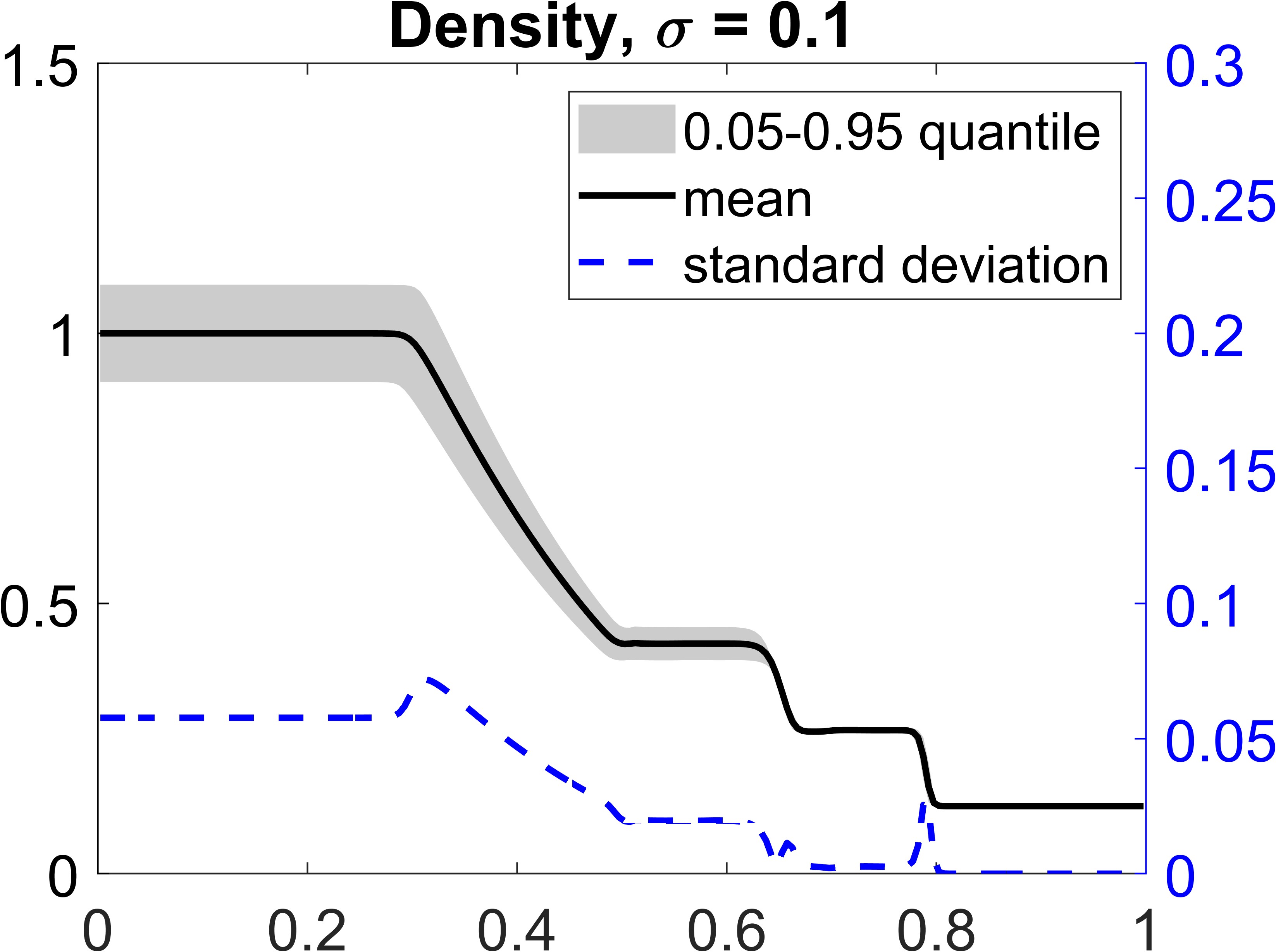
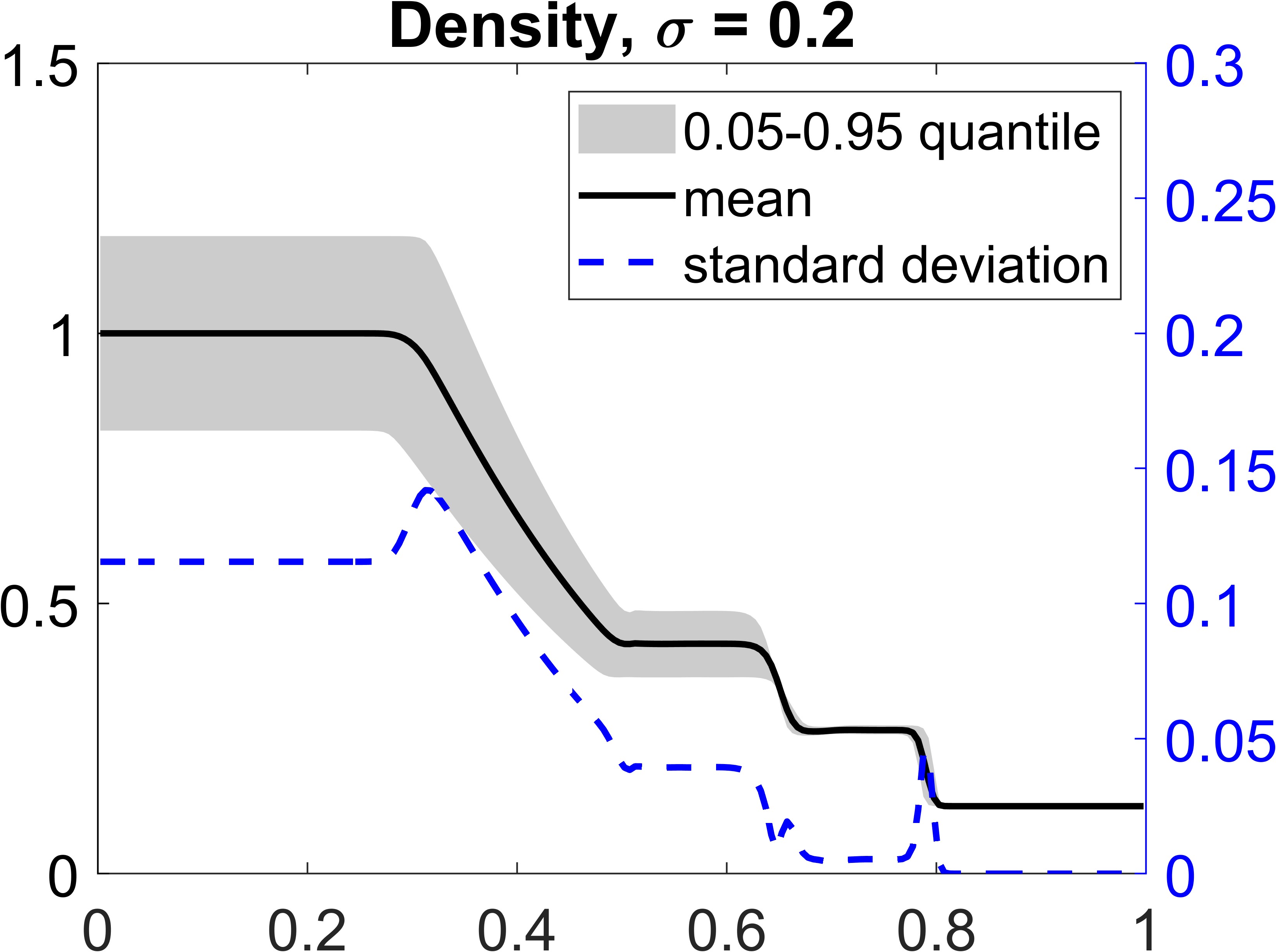
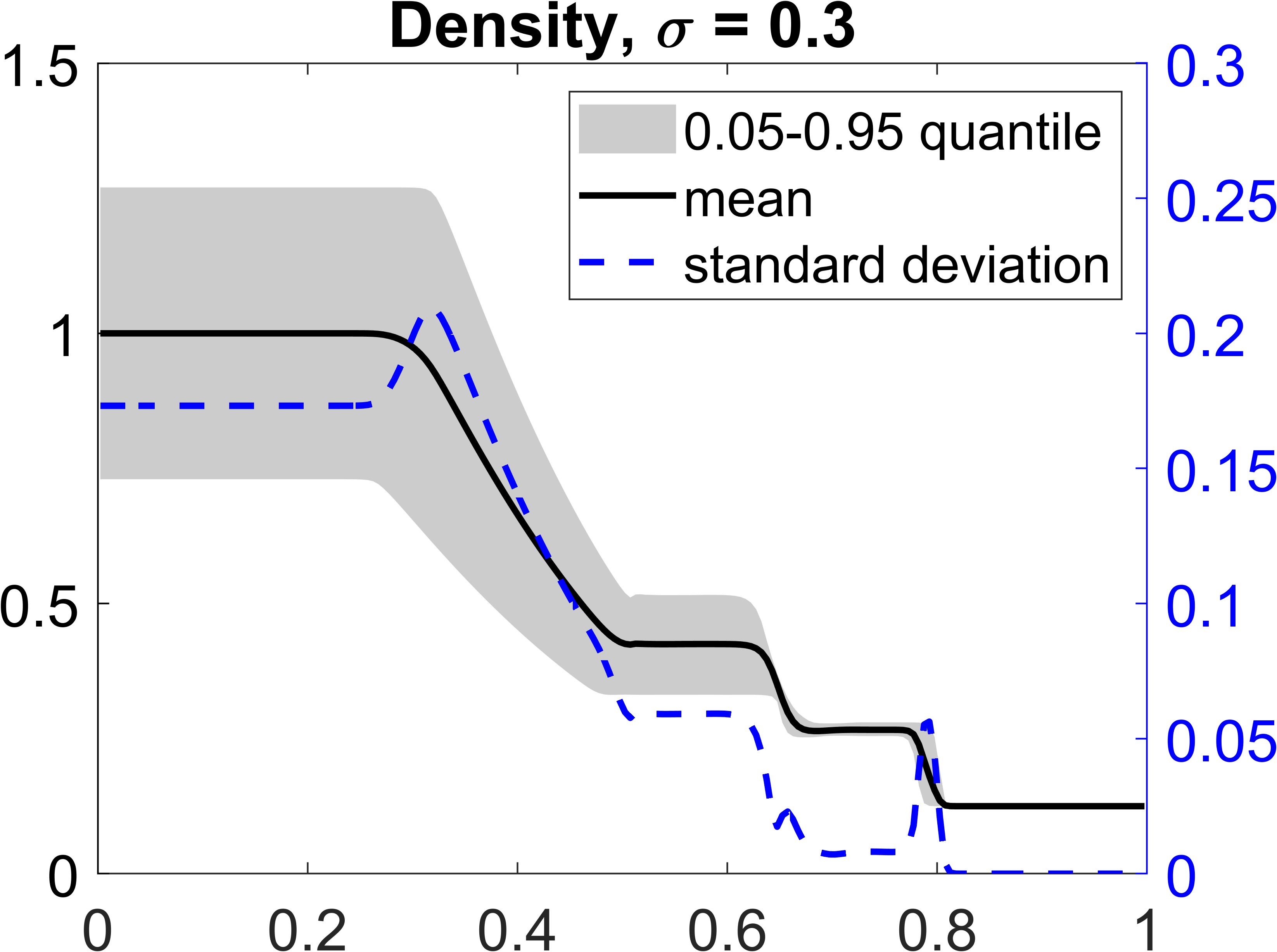
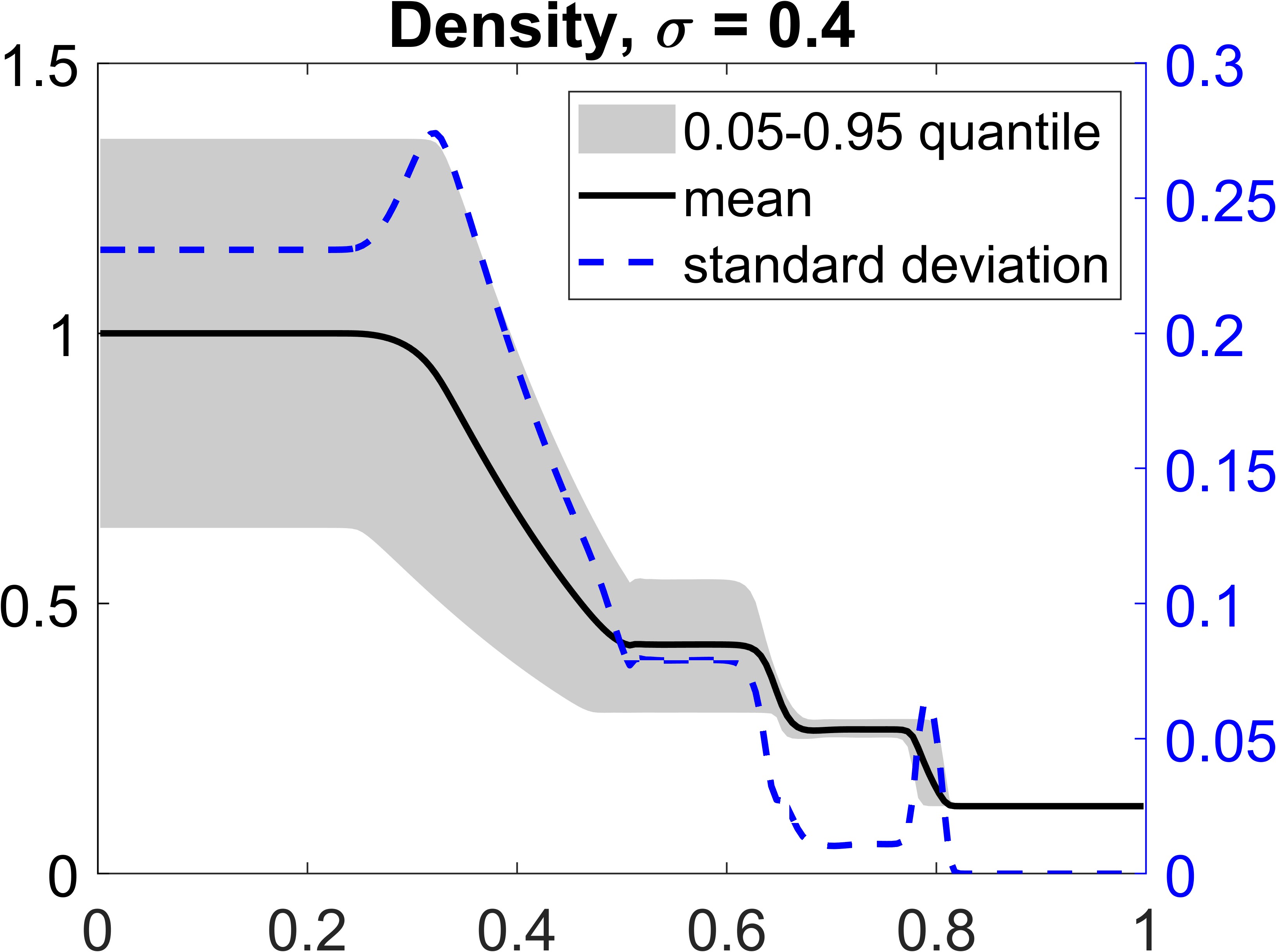
Figure 5.1: Example 1, Test 1: Mean, 95%-quantile, and standard deviation of $\rho$ for different $\sigma$.

It is also instructive to observe that the $95\%$-quantile in the momentum is distributed over a slightly different domain, while the $95\%$-quantile is almost invisible in the pressure and total energy; see Figure 5.2, where the corresponding results for $\sigma=0.1$ are plotted.

           

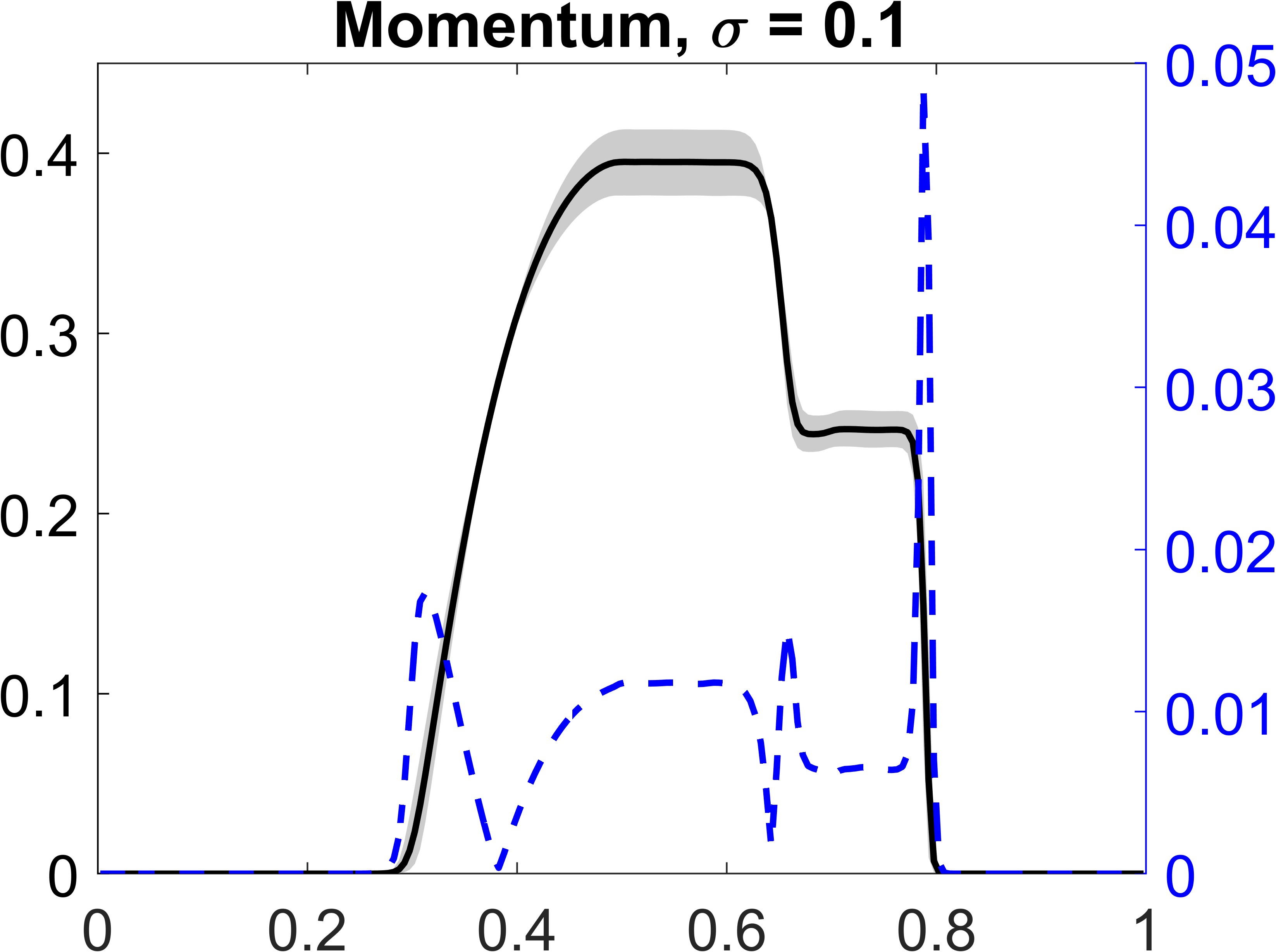
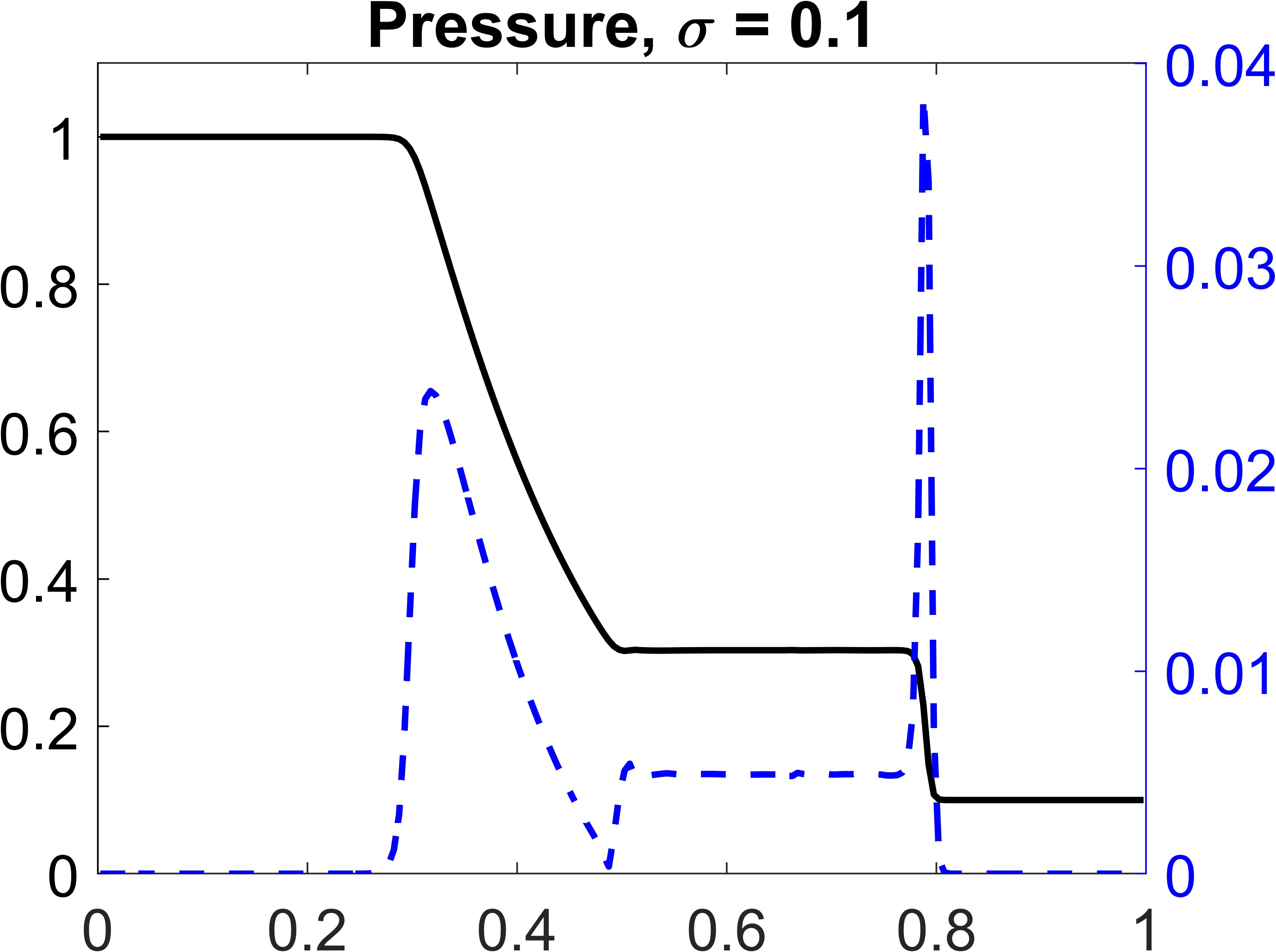
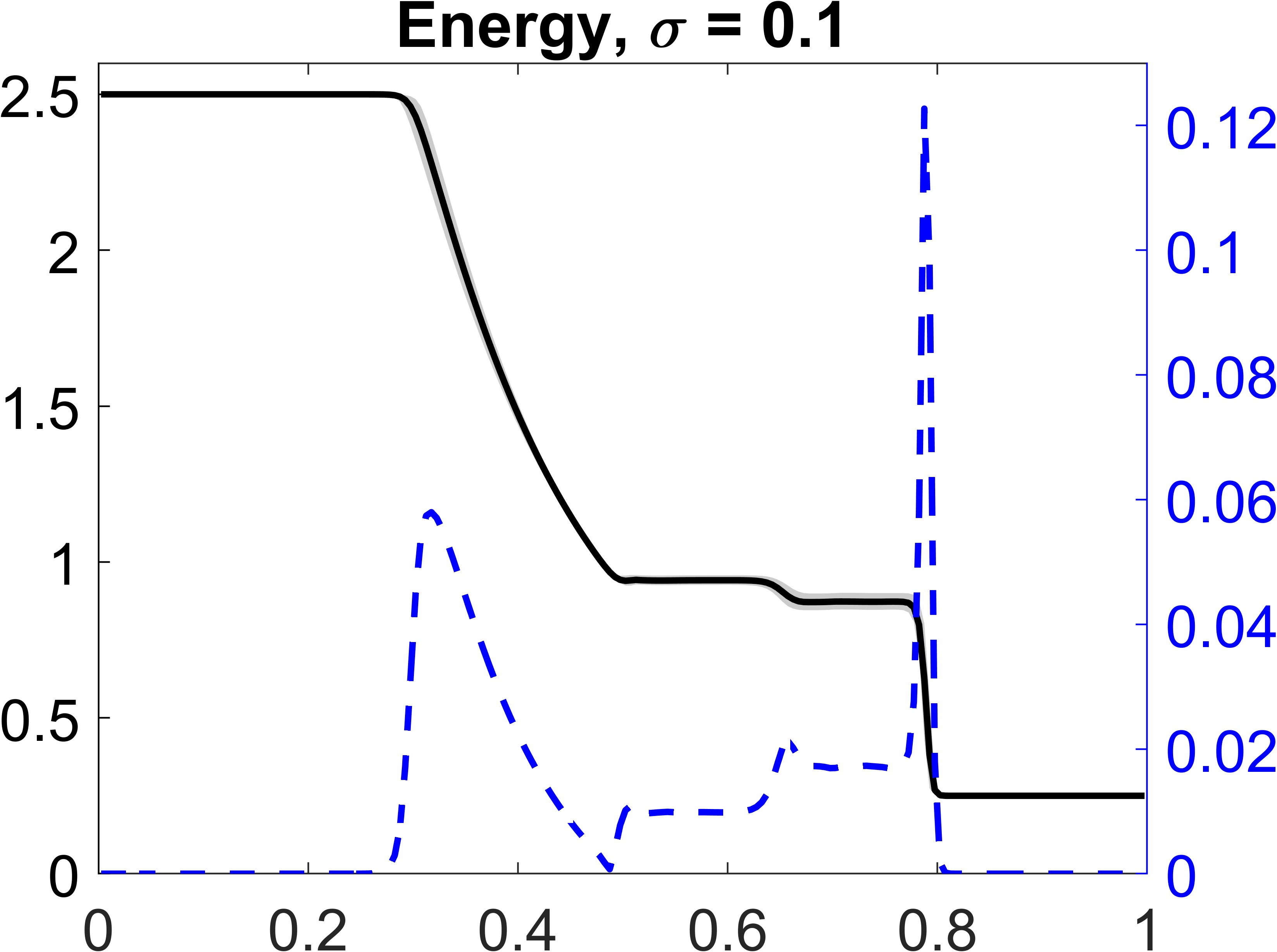
Figure 5.2: Example 1, Test 1: Mean, 95%-quantile, and standard deviation of $\rho u$, $p$, and $E$ for $\sigma=0.1$.

Test 2. Next, we consider the original Sod shock tube problem (5.3) with the uncertainty introduced in the adiabatic constant $\gamma$, which is now $\gamma(\xi)=1.4+0.1\xi$. It is easy to see that the perturbation of $\gamma$ affects the initial total energy only, and thus, one can expect that this perturbation will have the largest influence on the total energy. Indeed, this is true, as one can see in Figure 5.3, where we plot the mean, $95\%$ quantile, and standard deviation of $\rho$, $\rho u$, and $E$ computed on a uniform mesh with $\Delta x=1/200$ and $\Delta\xi=1/50$.

     

     

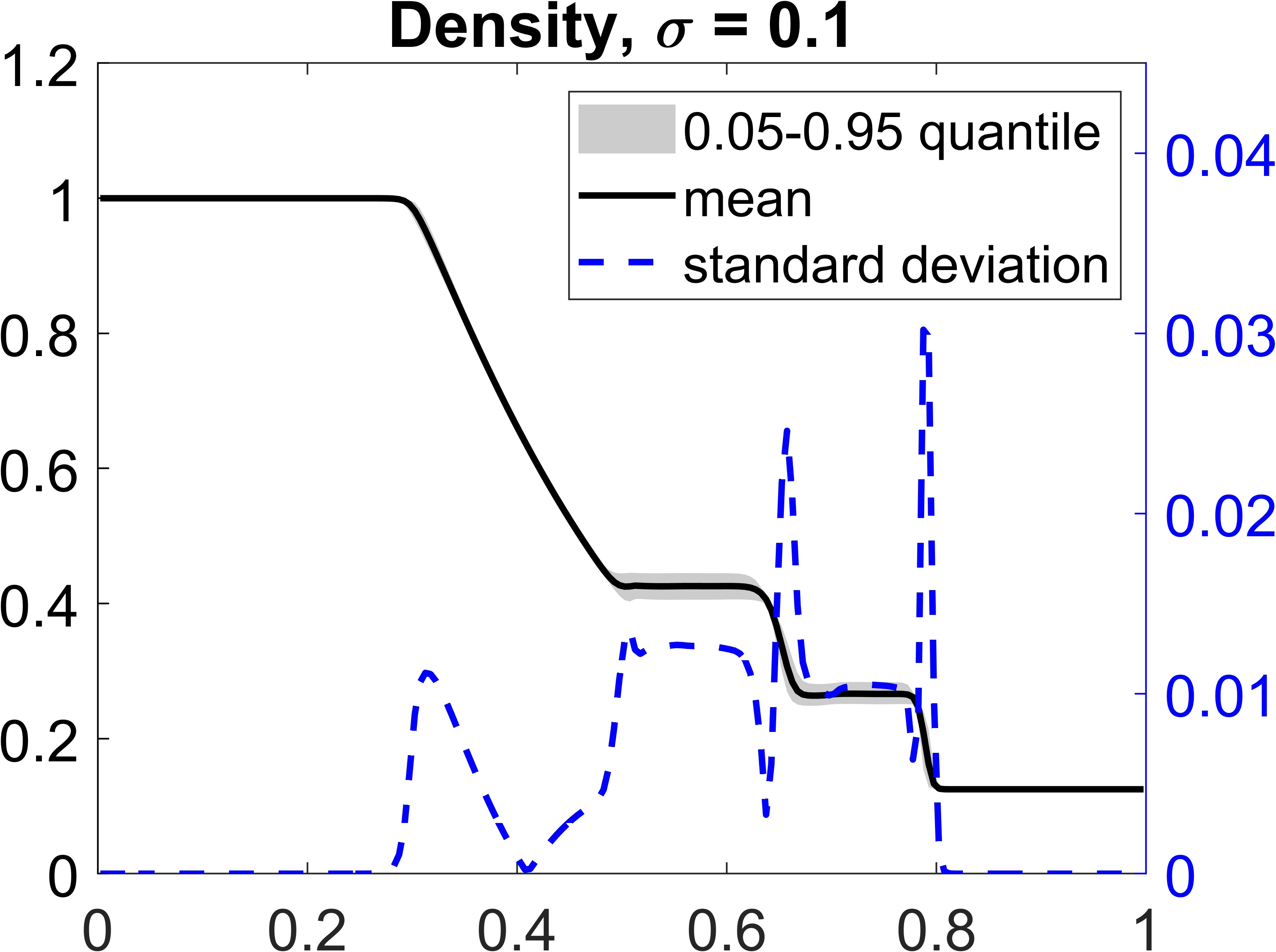
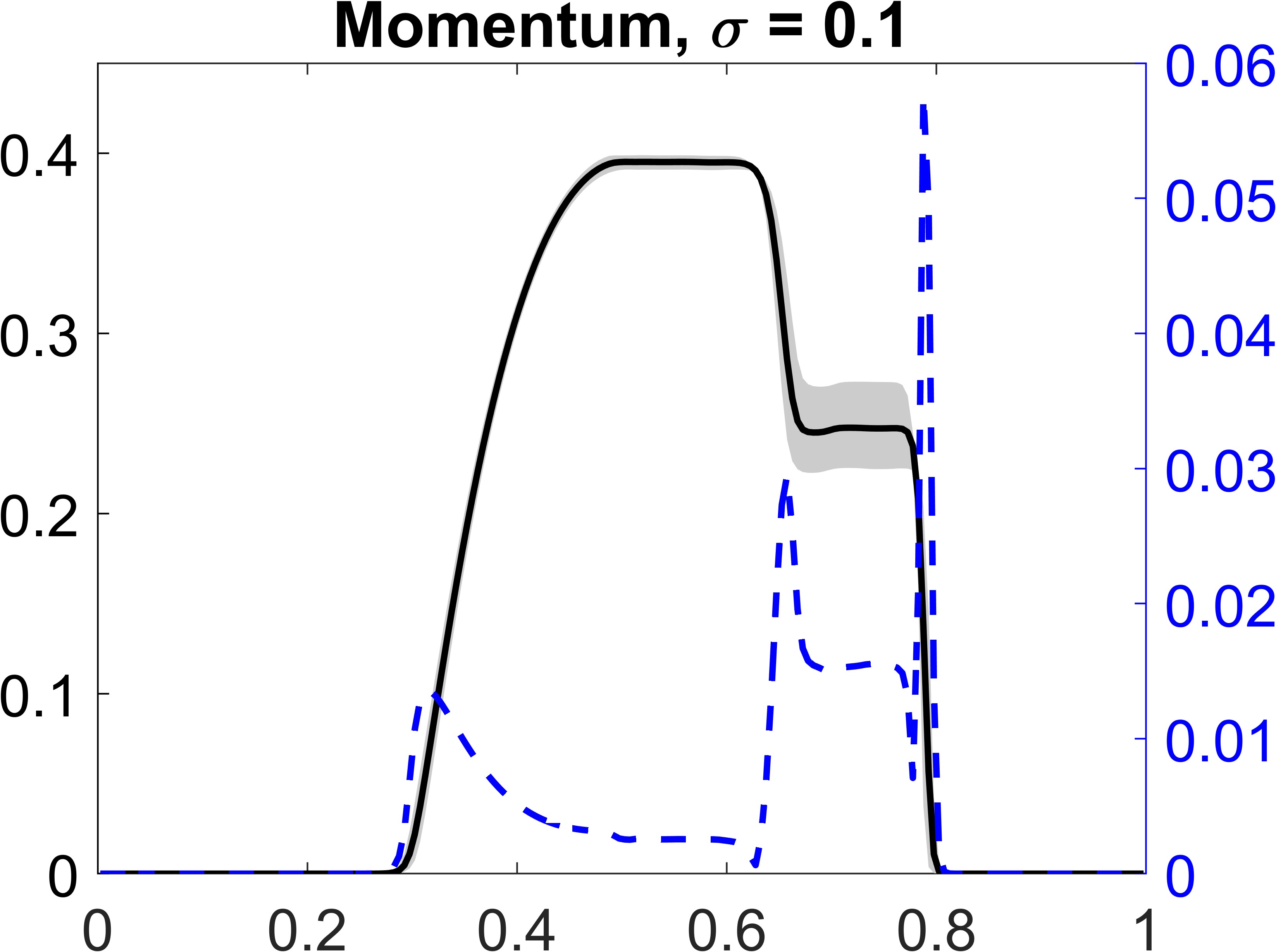
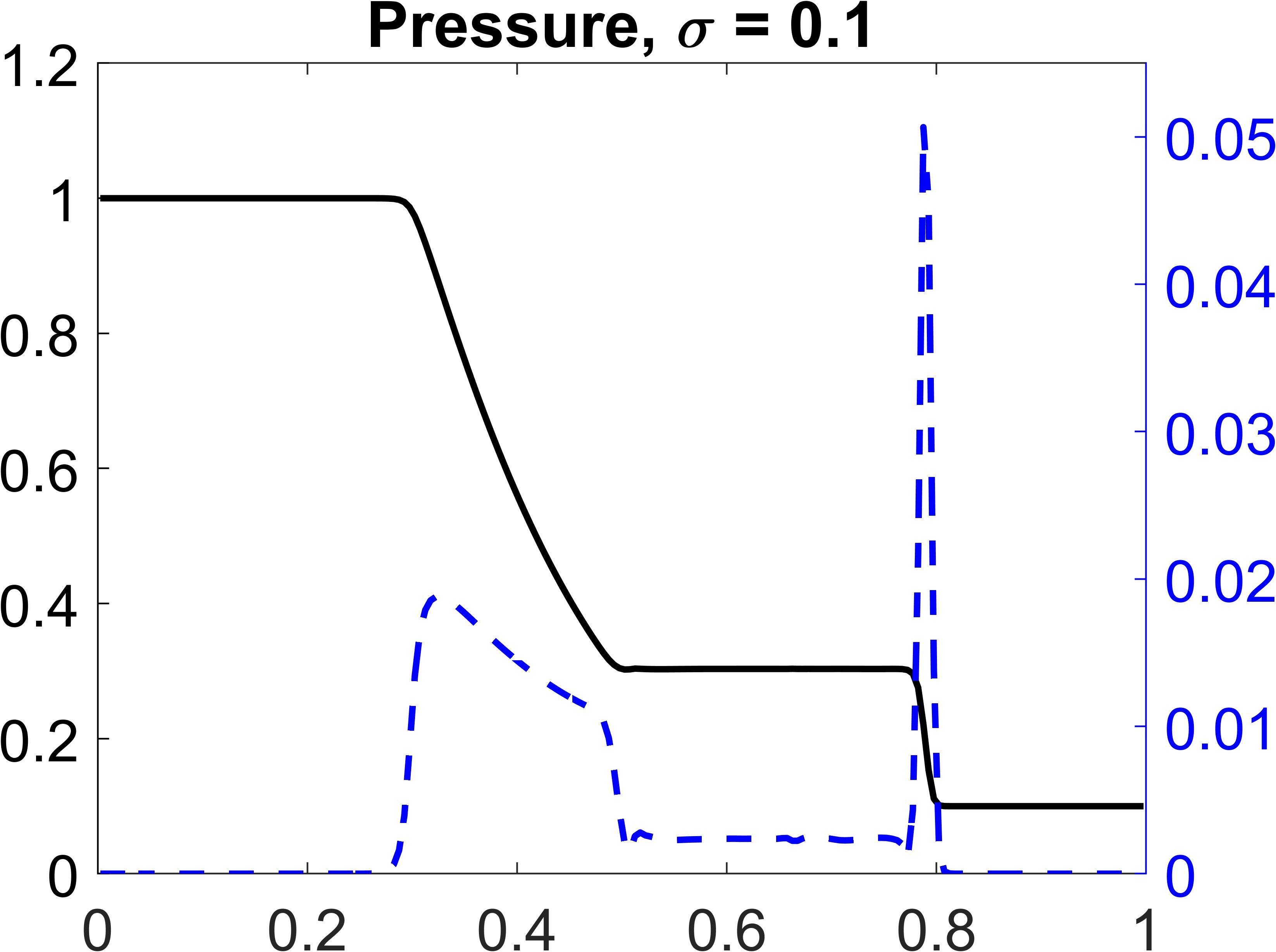
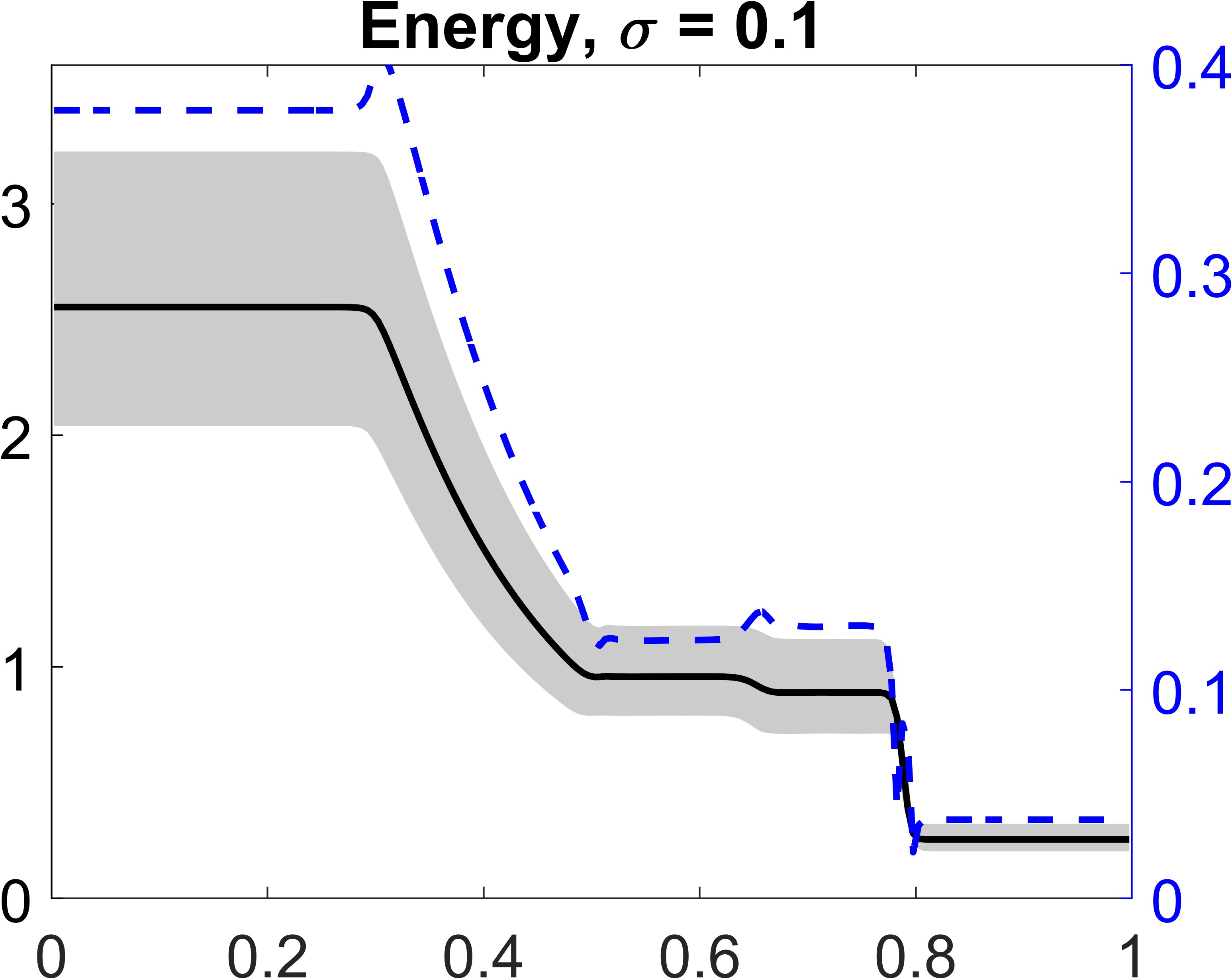
Figure 5.3: Example 1, Test 2: Mean, 95%-quantile, and standard deviation of $\rho$, $\rho u$, $p$, and $E$.

Example 2 ($d=1$ and $s=2$).

The second example corresponds to the case of one spatial variable $x$ and two random variables $\xi$ and $\eta$. In this case, the studied system is given by (2.1), (5.1), (5.2) but with all of the quantities depending not only on $x$, $\xi$, and $t$ but also on $\eta$.

We consider the same Sod shock tube problem (5.3) studied in Example 1, but with the uncertainties in both the ICs and adiabatic constant:

$$(\rho(x,0,\xi,\eta),u(x,0,\xi,\eta),p(x,0,\xi,\eta))=\left\{\begin{aligned} &(1+0.1\xi,0,1),&&x<0.5,\\ &(0.125,0,0.1),&&x>0.5,\end{aligned}\right.\qquad\gamma(\eta)=1.4+0.1\eta.$$

We compute the solution on a uniform mesh with $\Delta x=1/200$ and $\Delta\xi=\Delta\eta=1/50$. The obtained results are shown in Figure 5.4, where one can see the mean and standard deviation for $\rho$, $\rho u$, $p$, and $E$. These results confirm that the proposed numerical method can handle the case of multidimensional random variables.

     

     

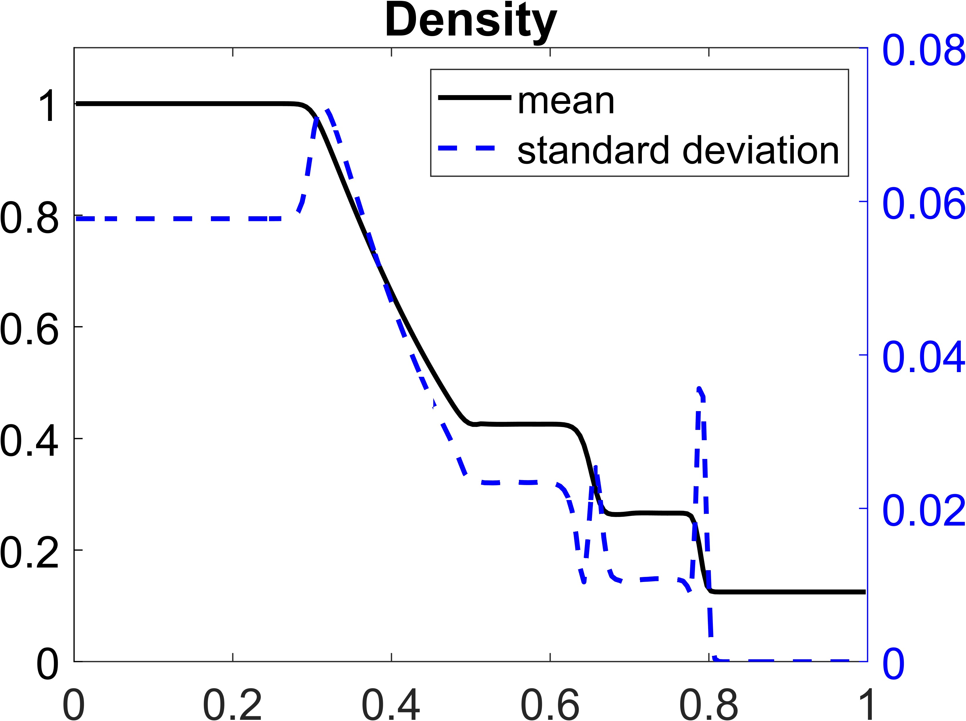
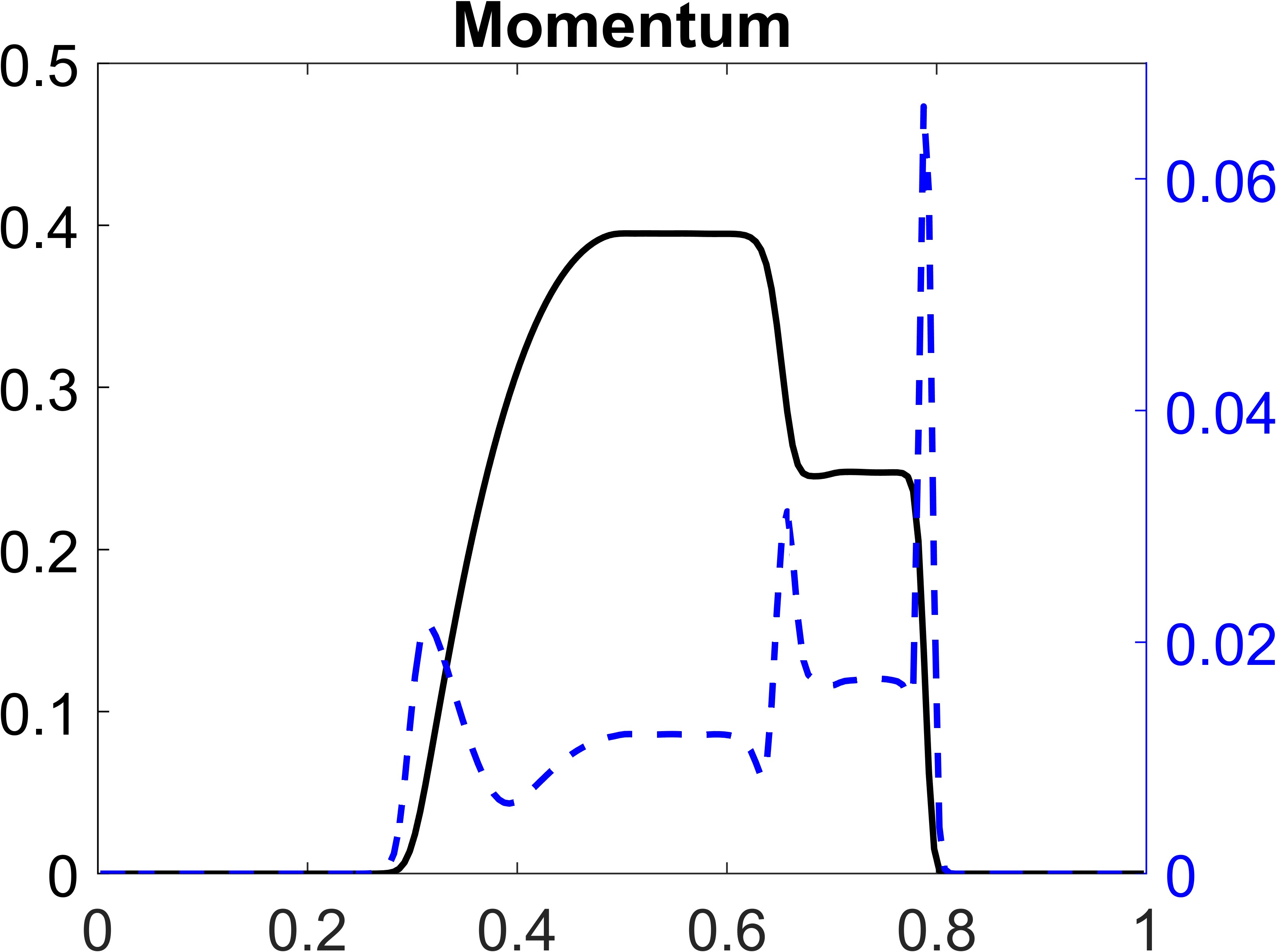
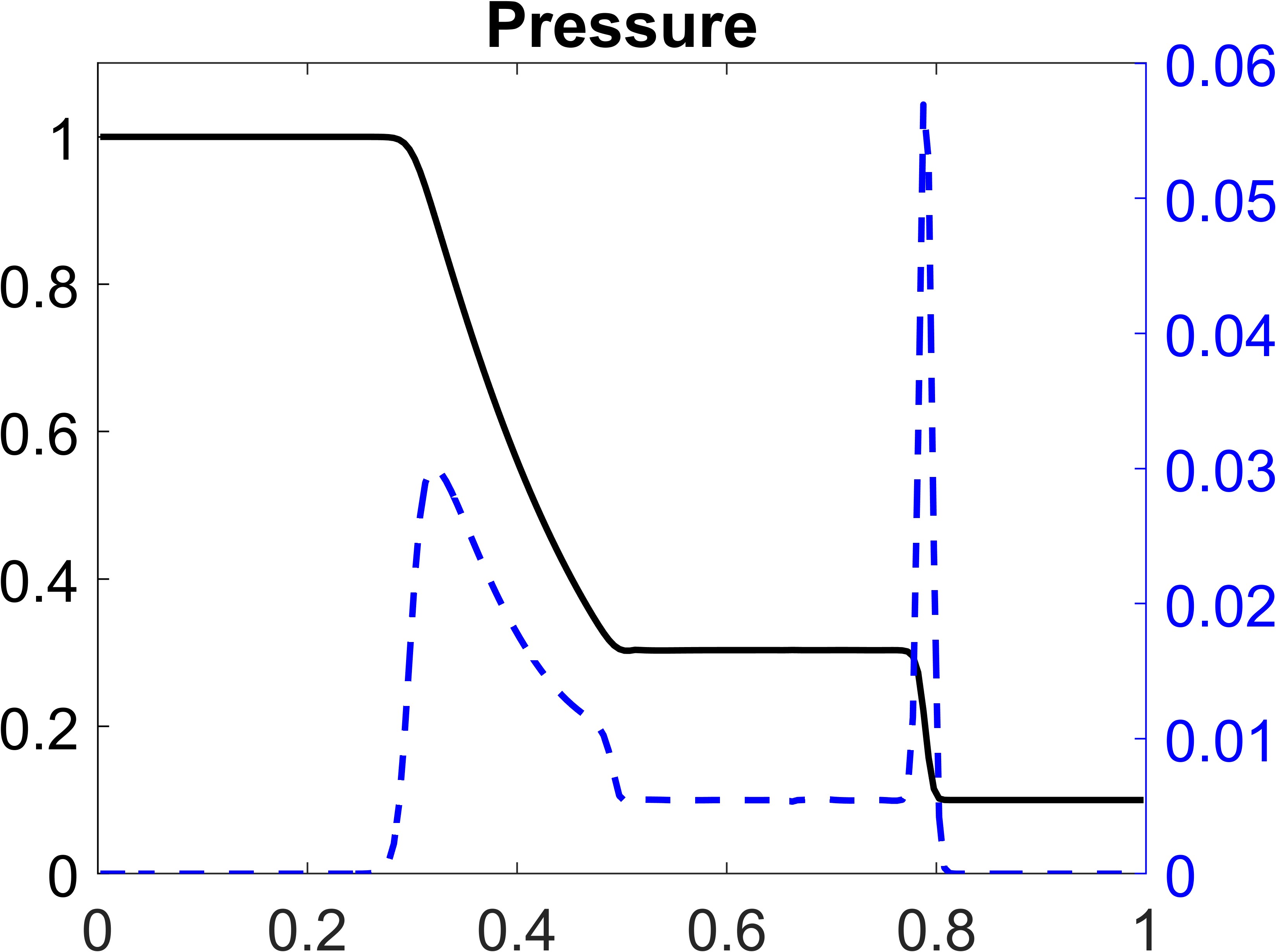
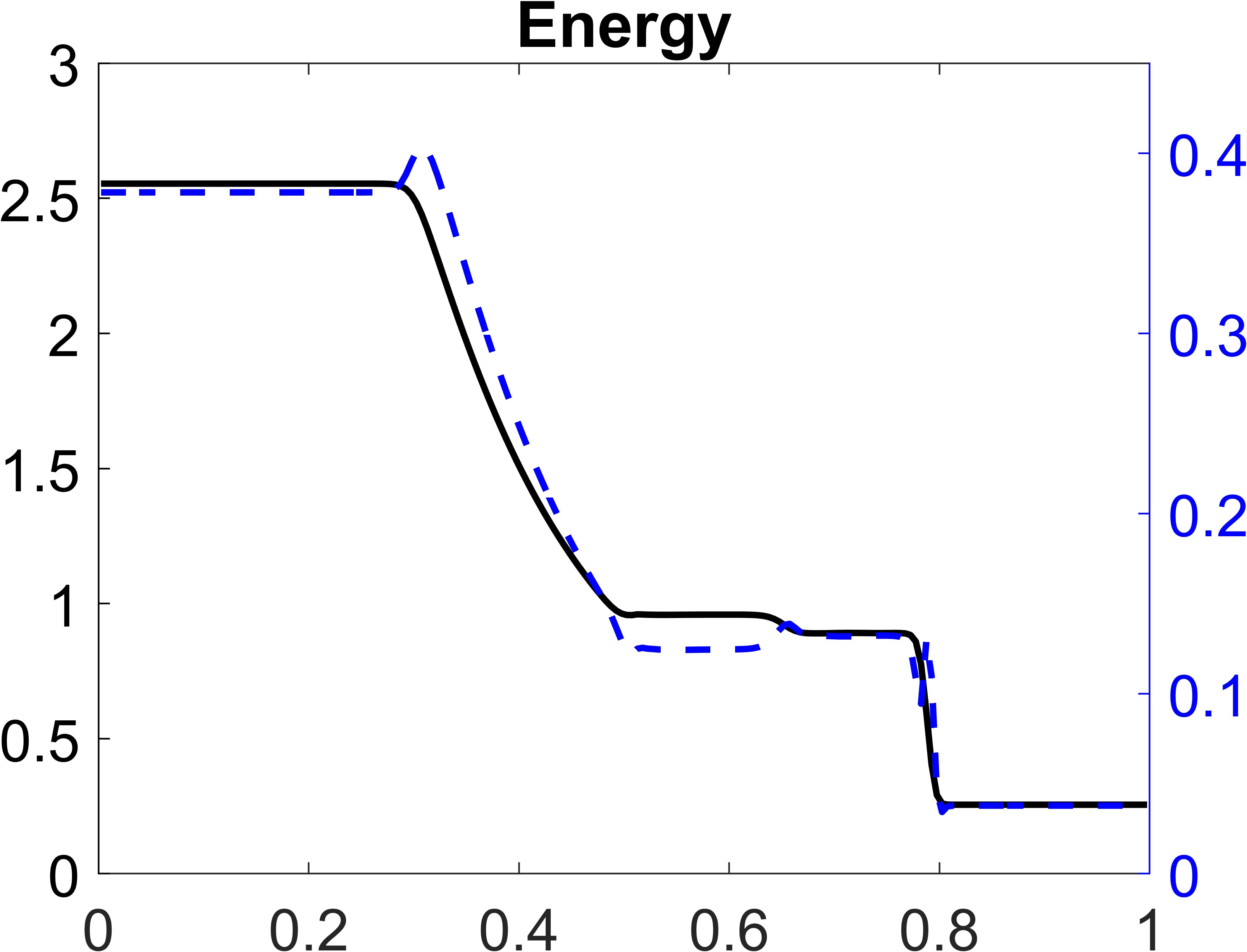
Figure 5.4: Example 2: Mean and standard deviation of $\rho$, $\rho u$, $p$, and $E$.

Example 3 ($d=2$ and $s=1$).

In the last numerical example, we consider the case of two spatial variables $x$ and $y$ and one random variable $\xi$, for which the Euler equations are governed by (3.8) with

$$\bm{U}=(\rho,\rho u,\rho v,E)^{\top},\quad\bm{F}(\bm{U})=\big{(}\rho u,\rho u^{2}+p,\rho uv,u(E+p)\big{)}^{\top},$$

$$\bm{G}(\bm{U})=(\rho v,\rho uv,\rho u^{2}+p,v(E+p))^{\top},\quad\bm{S}\equiv\bm{0},$$

supplemented with the EOS:

$$p=(\gamma-1)\left[E-\frac{\rho(u^{2}+v^{2})}{2}\right]$$

with $\gamma=1.4$. Here, $u(x,y,t,\xi)$ and $v(x,y,t,\xi)$ are the $x$- and $y$-velocity components, respectively.

For the ICs, we take a two-dimensional (2-D) Riemann problem, which is a perturbed (for nonzero $\sigma$) version of configuration 10 from [25]:

$$(\rho,u,v,p)(x,y,0,\xi)=\left\{\begin{aligned} &(1,0,0.4297(1-\sigma\xi),1),&&x>0.5,~{}y>0.5,\\ &(0.5(1+\sigma\xi),\sigma\xi,0.6076(1-\sigma\xi),1-\sigma\xi),&&x<0.5,~{}y>0.5,\\ &(0.2281(1+\sigma\xi),0,-0.6076(1+\sigma\xi),0.3333),&&x<0.5,~{}y<0.5,\\ &(0.4562,0,-0.4297(1+\sigma\xi),0.3333),&&x>0.5,~{}y<0.5.\end{aligned}\right.$$

We first compute the deterministic solution ($\sigma=0$) on the spatial domain $(x,y)\in[0,1]\times[0,1]$ until time $t=0.15$ on a uniform mesh with $\Delta x=\Delta y=1/400$. The resulting density component is shown in Figure 5.5 (left). We then use a quite large erturbation with $\sigma=0.5$ and repeat the same numerical experiment using $\Delta\xi=1/10$. The mean of the obtained density is quite different from the deterministic case; see Figure 5.5 (middle). We also present the computed standard deviation in Figure 5.5 (right), where one can see the areas in which the uncertainties influence the solution the most.

           

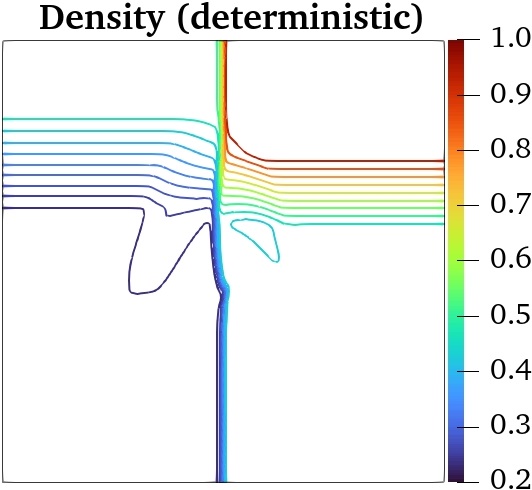
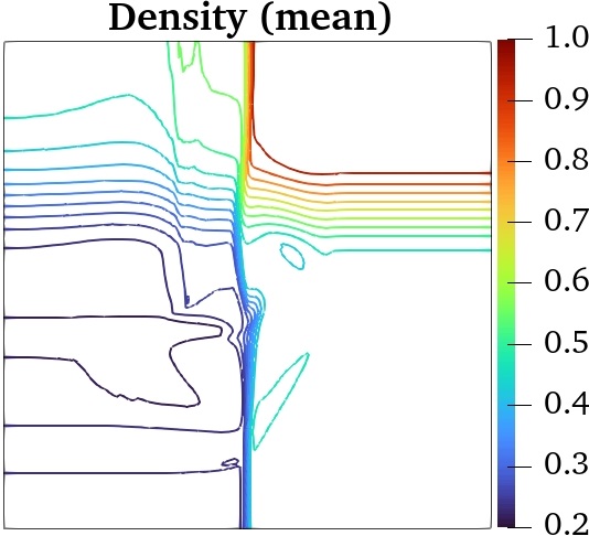
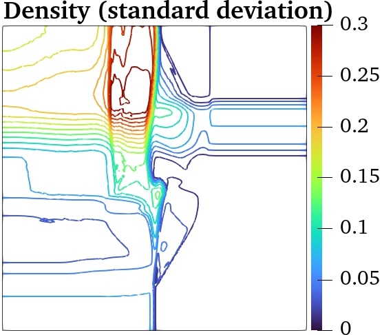
Figure 5.5: Example 3: Deterministic $\rho$ (left), and mean (middle) and standard deviation (right) of the uncertain $\rho$.

6 Saint-Venant System of Shallow Water Equations

We proceed by considering the Saint-Venant system of shallow water equations. There are several challenges associated with the numerical solution of the Saint-Venant system. First, it contains a geometric source term, which is balanced by the corresponding flux. This requires the development of the so-called WB schemes, which maintain this delicate balance at the discrete level. In addition, the water depth may naturally be very small or even zero, and thus a good numerical method must be able to guarantee the non-negativity of the computed water depth. The level of complexity increases even further with the presence of uncertainties as several additional techniques (compared to those presented in §2) need to be developed. In what follows, we adopt the approach introduced in [24] and extend it to the 1-D and 2-D Saint-Venant systems with uncertainties.

6.1 Case $d=1$ and $s=1$

We begin with the 1-D case, in which the Saint-Venant system is given by (2.1) with

$$\bm{U}=(h,hu)^{\top},\quad\bm{F}(\bm{U})=\Big{(}hu,hu^{2}+\frac{g}{2}h^{2}\Big{)}^{\top},\quad\bm{S}=(0,-ghZ_{x})^{\top},$$ (6.1)

where $h(x,t,\xi)$ is the water depth, $u(x,t,\xi)$ is the velocity, $Z(x,\xi)$ is a time-independent bottom topography, and $g$ is the constant acceleration due to gravity.

The system (2.1), (6.1) admits several steady states, among which the simplest ones are the so-called “lake-at-rest” equilibria:

$$u(x,\xi)\equiv 0,\quad w(x,\xi):=h(x,\xi)+Z(x,\xi)=\widehat{w}(\xi),$$ (6.2)

where $\widehat{w}$ is an arbitrary function of $\xi$ and the equilibrium variable $w$ represents the water surface. We will say that the scheme is WB if it is capable of preserving the “lake-at-rest” states (6.2) at the discrete level.

We follow the steps described in §2 to develop a scheme for (2.1), (6.1). However, in order to ensure the WB property, we do not reconstruct the point values of $h$—we instead reconstruct the water surface $w:=h+Z$. At the same time, we note that some of the point values $w^{+}_{{j-\frac{1}{2}},\ell_{i}}$ and $w^{-}_{{j+\frac{1}{2}},\ell_{i}}$, reconstructed using (2.10)–(2.12) followed by the Ai-WENO-Z interpolation introduced in §2.2.2, may not satisfy the water depth positivity requirement. We thus enforce the non-negativity of the point values of $h$ in the simplest way by setting

$$h^{+}_{{j-\frac{1}{2}},\ell_{i}}=\max\left\{w^{+}_{{j-\frac{1}{2}},\ell_{i}},Z_{{j-\frac{1}{2}},\ell_{i}}\right\}-Z_{{j-\frac{1}{2}},\ell_{i}},\quad h^{-}_{{j+\frac{1}{2}},\ell_{i}}=\max\left\{w^{-}_{{j+\frac{1}{2}},\ell_{i}},Z_{{j+\frac{1}{2}},\ell_{i}}\right\}-Z_{{j+\frac{1}{2}},\ell_{i}},$$

where $Z_{j\pm{\frac{1}{2}},\ell_{i}}:=Z(x_{j\pm{\frac{1}{2}}},\xi_{\ell_{i}})$.

Once the reconstructed point values of $h$ and $hu$ are available, we need to compute the corresponding point values of $u=\nicefrac{{(hu)}}{{h}}$. In order to avoid a division by small numbers, as $h$ may be very small, the computation of $u$ must be desingularized. We use the following desingularization formula (see [24]):

$$u=\frac{2h(hu)}{h^{2}+[\max(h,\varepsilon)]^{2}},$$ (6.3)

where $\varepsilon$ is a small positive number, taken $\varepsilon=10^{-6}$ is all of the numerical experiments reported below. For consistency, we then recalculate the corresponding point values of $hu$ by setting

$$(hu):=h\cdot u.$$ (6.4)

We note that all of the indexes in formulae (6.3) and (6.4) have been omitted for the sake of brevity.

Finally, we follow the lines of [24] and design a WB quadrature for the integral on the RHS of (2.7) of the second component of source term $\bm{S}$ in (6.1):

$$\int\limits_{x_{j-\frac{1}{2}}}^{x_{j+\frac{1}{2}}}\big{(}-gh(x,\xi_{\ell_{i}},t)Z_{x}(x,\xi_{\ell_{i}})\big{)}\,{\rm d}x\approx-\frac{g}{2}\big{(}h_{{j-\frac{1}{2}},\ell_{i}}^{+}+h_{{j+\frac{1}{2}},\ell_{i}}^{-}\big{)}\big{(}Z_{{j+\frac{1}{2}},\ell_{i}}-Z_{{j-\frac{1}{2}},\ell_{i}}\big{)}.$$ (6.5)

The use of the quadrature (6.5) in (2.7) leads to the WB semi-discrete scheme (2.2), (2.4)–(2.7), (6.5) as we prove in the following theorem.

Theorem 6.1.

Assume that at a certain time level, the discrete solution is at a “lake-at-rest” steady state, that is,

$$\hbox{\vbox{\hrule height=0.5pt\kern 1.72218pt\hbox{\kern-0.50003pt$w$\kern 0.0pt}}}_{j,\ell}=\,\hbox{\vbox{\hrule height=0.5pt\kern 1.72218pt\hbox{\kern-0.50003pt$h$\kern 0.0pt}}}_{j,\ell}+\hbox{\vbox{\hrule height=0.5pt\kern 1.72218pt\hbox{\kern-0.50003pt$Z$\kern 0.0pt}}}_{j,\ell}\equiv\widehat{w}_{\ell},\quad(\hbox{\vbox{\hrule height=0.5pt\kern 1.72218pt\hbox{\kern-0.50003pt$hu$\kern 0.0pt}}})_{j,\ell}\equiv 0,\quad\forall j,\ell.$$

Then, the RHS of the system of ODEs (2.2) vanishes and hence the proposed semi-discrete scheme (2.2), (2.4)–(6.5), (6.5) is WB.

Proof.

We first observe that the minmod reconstruction in the $x$-direction (2.10)–(2.12) ensures

$$w^{-}_{{j+\frac{1}{2}},\ell}=w^{+}_{{j+\frac{1}{2}},\ell}=\widehat{w}_{\ell},\quad u^{-}_{{j+\frac{1}{2}},\ell}=u^{+}_{{j+\frac{1}{2}},\ell}=0,\quad\forall j,\ell.$$ (6.6)

Then, the fifth-order Ai-WENO-Z interpolation described in §2.2.2 results in

$$\begin{aligned} &w^{-}_{{j+\frac{1}{2}},\ell+\kappa}=w^{+}_{{j+\frac{1}{2}},\ell+\kappa}=w_{\ell+\kappa},\\ &w^{-}_{{j+\frac{1}{2}},\ell-\kappa}=w^{+}_{{j+\frac{1}{2}},\ell-\kappa}=w_{\ell-\kappa},\end{aligned}\qquad u^{-}_{{j+\frac{1}{2}},\ell\pm\kappa}=u^{+}_{{j+\frac{1}{2}},\ell\pm\kappa}=0,\quad\forall j,\ell,$$ (6.7)

where the values $w_{\ell\pm\kappa}$ are independent of $j$ since for the “lake-at-rest” data, the Ai-WENO-Z interpolation is conducted over the same set of discrete values along $x=x_{j+\frac{1}{2}},\,\forall j$.

Using (6.6) and (6.7) in (2.4)–(2.5) and (2.7), (6.5), we obtain the following formula for the CU numerical fluxes $\bm{{\cal F}}_{{j+\frac{1}{2}},\ell}=({\cal F}^{(1)}_{{j+\frac{1}{2}},\ell},{\cal F}^{(2)}_{{j+\frac{1}{2}},\ell})^{\top}$:

$${\cal F}^{(1)}_{{j+\frac{1}{2}},\ell}=0,$$ (6.8)

$${\cal F}^{(2)}_{{j+\frac{1}{2}},\ell}=\frac{\mu_{1}g}{2}\big{(}w_{\ell-\kappa}-Z_{{j+\frac{1}{2}},\ell-\kappa}\big{)}^{2}+\frac{\mu_{2}g}{2}\big{(}\widehat{w}_{\ell}-Z_{{j+\frac{1}{2}},\ell}\big{)}^{2}+\frac{\mu_{3}g}{2}\big{(}w_{\ell+\kappa}-Z_{{j+\frac{1}{2}},\ell+\kappa}\big{)}^{2},$$

and the source term $\bm{S}_{j,\ell}=(0,S^{(2)}_{j,\ell})^{\top}$:

$$S^{(2)}_{j,\ell}= -\frac{\mu_{1}g}{2}\big{(}2w_{\ell-\kappa}-Z_{{j+\frac{1}{2}},\ell-\kappa}-Z_{{j-\frac{1}{2}},\ell-\kappa}\big{)}\big{(}Z_{{j+\frac{1}{2}},\ell-\kappa}-Z_{{j-\frac{1}{2}},\ell-\kappa}\big{)}$$ (6.9)

$$-\frac{\mu_{2}g}{2}\big{(}2\widehat{w}_{\ell}-Z_{{j+\frac{1}{2}},\ell}-Z_{{j-\frac{1}{2}},\ell}\big{)}\big{(}Z_{{j+\frac{1}{2}},\ell}-Z_{{j-\frac{1}{2}},\ell}\big{)}$$

$$-\frac{\mu_{3}g}{2}\big{(}2w_{\ell+\kappa}-Z_{{j+\frac{1}{2}},\ell+\kappa}-Z_{{j-\frac{1}{2}},\ell+\kappa}\big{)}\big{(}Z_{{j+\frac{1}{2}},\ell+\kappa}-Z_{{j-\frac{1}{2}},\ell+\kappa}\big{)}.$$

Substituting (6.8) and (6.9) into (2.2) and using a simplifying the obtained expressions, yields

$$\frac{{\rm d}}{{\rm d}t}\,\hbox{\vbox{\hrule height=0.5pt\kern 1.72218pt\hbox{\kern-0.50003pt$\bm{U}$\kern 0.0pt}}}_{j,\ell}(t)=\bm{0},$$

which completes the proof of the theorem. ∎

6.2 Case $d=1$ and $s=2$

We now consider the Saint-Venant system (2.1), (6.1), where all of the quantities depend on two independent random variables $\xi$ and $\eta$ in addition to the dependence on the physical variables $x$ and $t$. In this case, the “lake-at-rest” equilibria are given by

$$u(x,\xi,\eta)\equiv 0,\quad w(x,\xi,\eta):=h(x,\xi,\eta)+Z(x,\xi,\eta)=\widehat{w}(\xi,\eta),$$

where $\widehat{w}$ is now an arbitrary function of both $\xi$ and $\eta$.

As in §6.1, we reconstruct $w$ and $hu$ and then obtain the non-negative point values of $h$ by setting

$$h^{+}_{{j-\frac{1}{2}},\ell_{i},m_{r}}=\max\left\{w^{+}_{{j-\frac{1}{2}},\ell_{i},m_{r}},Z_{{j-\frac{1}{2}},\ell_{i},m_{r}}\right\}-Z_{{j-\frac{1}{2}},\ell_{i},m_{r}},$$

$$h^{-}_{{j+\frac{1}{2}},\ell_{i},m_{r}}=\max\left\{w^{-}_{{j+\frac{1}{2}},\ell_{i},m_{r}},Z_{{j+\frac{1}{2}},\ell_{i},m_{r}}\right\}-Z_{{j+\frac{1}{2}},\ell_{i},m_{r}},$$

where $Z_{j\pm{\frac{1}{2}},\ell_{i},m_{r}}:=Z(x_{j\pm{\frac{1}{2}}},\xi_{\ell_{i}},\eta_{m_{r}})$, and desingularize the computation of the point values of $u$ using (6.3) and (6.4). Finally, the WB quadrature (6.5) now reads as

$$\int\limits_{x_{j-\frac{1}{2}}}^{x_{j+\frac{1}{2}}}\big{(} -gh(x,\xi_{\ell_{i}},\eta_{m_{r}}t)Z_{x}(x,\xi_{\ell_{i}},\eta_{m_{r}})\big{)}\,{\rm d}x$$ (6.10)

$$\approx -\frac{g}{2}\big{(}h_{{j-\frac{1}{2}},\ell_{i},m_{r}}^{+}+h_{{j+\frac{1}{2}},\ell_{i},m_{r}}^{-}\big{)}\big{(}Z_{{j+\frac{1}{2}},\ell_{i},m_{r}}-Z_{{j-\frac{1}{2}},\ell_{i},m_{r}}\big{)}.$$

The use of the quadrature (6.10) in (3.6) leads to the WB semi-discrete scheme (3.2)–(3.6), (6.10), as stated in the following Theorem 6.2, whose proof is completely analogous to the proof of Theorem 6.1.

Theorem 6.2.

Assume that at a certain time level, the discrete solution is at a “lake-at-rest” steady state, that is,

$$\hbox{\vbox{\hrule height=0.5pt\kern 1.72218pt\hbox{\kern-0.50003pt$w$\kern 0.0pt}}}_{j,\ell,m}=\hbox{\vbox{\hrule height=0.5pt\kern 1.72218pt\hbox{\kern-0.50003pt$h$\kern 0.0pt}}}_{j,\ell,m}+\hbox{\vbox{\hrule height=0.5pt\kern 1.72218pt\hbox{\kern-0.50003pt$Z$\kern 0.0pt}}}_{j,\ell,m}\equiv\widehat{w}_{\ell,m},\quad(\hbox{\vbox{\hrule height=0.5pt\kern 1.72218pt\hbox{\kern-0.50003pt$hu$\kern 0.0pt}}})_{j,\ell,m}\equiv 0,\quad\forall j,\ell,m.$$

Then, the RHS of the system of ODEs (3.7) vanishes and hence the proposed semi-discrete scheme (3.2)–(3.6), (6.10) is WB.

6.3 Case $d=2$ and $s=1$

In this section, we consider a 2-D physical domain and one random variable $\xi$. The shallow water equations are given by (3.8) with

$$\bm{U}=(h,hu,hv)^{\top},\quad\bm{F}(\bm{U})=\Big{(}hu,hu^{2}+\frac{g}{2}h^{2},huv\Big{)}^{\top},$$ (6.11)

$$\bm{G}(\bm{U})=\Big{(}hv,huv,hv^{2}+\frac{g}{2}h^{2}\Big{)}^{\top},\quad\bm{S}=(0,-ghZ_{x},-ghZ_{y})^{\top},$$

where $h(x,y,\xi,t)$ is the water depth, $u(x,y,\xi,t)$ and $v(x,y,\xi,t)$ are the $x$- and $y$-velocities, $Z(x,y,\xi)$ is the bottom topography and $g$ is the constant acceleration due to gravity.

The system (1.1), (6.11) also admits the “lake-at-rest” steady states satisfying

$$u(x,y,\xi)=v(x,y,\xi)\equiv 0,\quad w(x,y,\xi)=\widehat{w}(\xi),$$

where $\widehat{w}$ is an arbitrary function of $\xi$.

As in the 1-D case, in order to develop a WB scheme for (3.8), (6.11), we first reconstruct the point values of $w$ and then calculate the point values of $h$ by enforcing their non-negativity through

$$h^{+}_{{j-\frac{1}{2}},k,\ell_{i}}=\max\left\{w^{+}_{{j-\frac{1}{2}},k,\ell_{i}},Z_{{j-\frac{1}{2}},k,\ell_{i}}\right\}-Z_{{j-\frac{1}{2}},k,\ell_{i}},$$

$$h^{-}_{{j+\frac{1}{2}},k,\ell_{i}}=\max\left\{w^{-}_{{j+\frac{1}{2}},k,\ell_{i}},Z_{{j+\frac{1}{2}},k,\ell_{i}}\right\}-Z_{{j+\frac{1}{2}},k,\ell_{i}},$$

$$h^{+}_{j,{k-\frac{1}{2}},\ell_{i}}=\max\left\{w^{+}_{j,{k-\frac{1}{2}},\ell_{i}},Z_{j,{k-\frac{1}{2}},\ell_{i}}\right\}-Z_{j,{k-\frac{1}{2}},\ell_{i}},$$

$$h^{-}_{j,{k+\frac{1}{2}},\ell_{i}}=\max\left\{w^{-}_{j,{k+\frac{1}{2}},\ell_{i}},Z_{j,{k+\frac{1}{2}},\ell_{i}}\right\}-Z_{j,{k+\frac{1}{2}},\ell_{i}},$$

where $Z_{j\pm{\frac{1}{2}},k,\ell_{i}}:=Z(x_{j\pm{\frac{1}{2}}},y_{k},\xi_{\ell_{i}})$ and $Z_{j,k\pm{\frac{1}{2}},\ell_{i}}:=Z(x_{j},y_{k\pm{\frac{1}{2}}},\xi_{\ell_{i}})$.

Once the reconstructed point values of $h,hu$, and $hv$ are available, we compute the corresponding point values of $u$ and $v$ by implementing the same desingularization procedure as in (6.3):

$$u=\frac{2h(hu)}{h^{2}+[\max(h,\varepsilon)]^{2}},\quad v=\frac{2h(hv)}{h^{2}+[\max(h,\varepsilon)]^{2}}$$ (6.12)

with a small positive parameter $\varepsilon$ taken to be $10^{-6}$ in the numerical experiment reported below. For consistency, we then recalculate the corresponding point values of $hu$ and $hv$ by setting

$$(hu):=h\cdot u,\quad(hv):=h\cdot v.$$ (6.13)

As before, the indexes in formulae (6.12) and (6.13) have been omitted for the sake of brevity.

We complete the construction of the scheme by designing a WB quadrature for the integral on the RHS of (3.13) of the second and third components of source term $\bm{S}$ in (6.11). As in the 1-D case, we follow the lines of [24] and obtain

$$\int\limits_{y_{k-\frac{1}{2}}}^{y_{k+\frac{1}{2}}}\int\limits_{x_{j-\frac{1}{2}}}^{x_{j+\frac{1}{2}}}\big{(} -gh(x,y,\xi_{\ell_{i}},t)Z_{x}(x,y,\xi_{\ell_{i}})\big{)}\,{\rm d}x\,{\rm d}y$$ (6.14)

$$\approx -\frac{g\Delta y}{2}\big{(}h_{{j-\frac{1}{2}},k,\ell_{i}}^{+}+h_{{j+\frac{1}{2}},k,\ell_{i}}^{-}\big{)}\big{(}Z_{{j+\frac{1}{2}},k,\ell_{i}}-Z_{{j-\frac{1}{2}},k,\ell_{i}}\big{)},$$

$$\int\limits_{y_{k-\frac{1}{2}}}^{y_{k+\frac{1}{2}}}\int\limits_{x_{j-\frac{1}{2}}}^{x_{j+\frac{1}{2}}}\big{(} -gh(x,y,\xi_{\ell_{i}},t)Z_{y}(x,y,\xi_{\ell_{i}})\big{)}\,{\rm d}x\,{\rm d}y$$

$$\approx -\frac{g\Delta x}{2}\big{(}h_{j,{k-\frac{1}{2}},\ell_{i}}^{+}+h_{j,{k+\frac{1}{2}},\ell_{i}}^{-}\big{)}\big{(}Z_{j,{k+\frac{1}{2}},\ell_{i}}-Z_{j,{k-\frac{1}{2}},\ell_{i}}\big{)}.$$

The use of the quadrature (6.14) in (3.13) leads to the WB semi-discrete scheme (3.9)–(3.13), (6.14) as stated in the Theorem 6.3, whose proof is similar to the proof of Theorem 6.1 and thus omitted for the sake of brevity.

Theorem 6.3.

Assume that at a certain time level, the discrete solution is at a “lake-at-rest” steady state, that is,

$$\hbox{\vbox{\hrule height=0.5pt\kern 1.72218pt\hbox{\kern-0.50003pt$w$\kern 0.0pt}}}_{j,k,\ell}=\hbox{\vbox{\hrule height=0.5pt\kern 1.72218pt\hbox{\kern-0.50003pt$h$\kern 0.0pt}}}_{j,k,\ell}+\hbox{\vbox{\hrule height=0.5pt\kern 1.72218pt\hbox{\kern-0.50003pt$Z$\kern 0.0pt}}}_{j,k,\ell}\equiv\widehat{w}_{\ell},\quad(\hbox{\vbox{\hrule height=0.5pt\kern 1.72218pt\hbox{\kern-0.50003pt$hu$\kern 0.0pt}}})_{j,k,\ell}=(\hbox{\vbox{\hrule height=0.5pt\kern 1.72218pt\hbox{\kern-0.50003pt$hv$\kern 0.0pt}}})_{j,k,\ell}\equiv 0,\quad\forall j,k,\ell.$$

Then, the RHS of the system of ODEs (3.2) vanishes and hence the proposed semi-discrete scheme (3.9)–(3.13), (6.14) is WB.

6.4 Numerical Examples

In this section, we illustrate the performance of the proposed numerical method on several examples for the Saint-Venant system. In all of the examples, we take $g=1$, except for Example 7, in which we take $g=9.812$. As before, we assume that the random variables $\xi,\eta$ are uniformly distributed on $[-1,1]$. We have used the minmod parameter either $\theta=1$ (Examples 4 and 7) or $\theta=1.3$ (Examples 5, 6, and 8).

Example 4 (Accuracy Test, $d=s=1$).

We begin with experimentally verifying the fifth order of accuracy in $\xi$ of the proposed finite-volume method. To this end, we consider the following smooth ICs with uncertainty in the water surface:

$$w(x,0,\xi)=1+0.1\tanh(4\xi)+0.01\sin(2\pi x),\quad u(x,0,\xi)\equiv 0.1.$$

We take a flat bottom topography $Z(x,\xi)\equiv 0$ and impose periodic BCs on the spatial domain $x\in[0,1]$.

We compute the numerical solution until time $t=0.01$ (at which the solution is still smooth) on a sequence of uniform meshes with $\Delta\xi=2/16$, $2/32$, $2/64$, and $2/128$. We then estimate the $L^{1}$-errors and experimental convergence rates using the following Runge formulae, which are based on the solutions computed on the three consecutive uniform grids with the mesh sizes $\Delta\xi$, $2\Delta\xi$, and $4\Delta\xi$ and denoted by $(\cdot)^{\Delta\xi}$, $(\cdot)^{2\Delta\xi}$, and $(\cdot)^{4\Delta\xi}$, respectively:

$${\rm Error}(\Delta\xi)\approx\frac{\delta^{2}_{12}}{|\delta_{12}-\delta_{24}|},\quad{\rm Rate}(\Delta\xi)\approx\log_{2}\left(\frac{\delta_{24}}{\delta_{12}}\right).$$

Here, $\delta_{12}:=\|(\cdot)^{\Delta\xi}-(\cdot)^{2\Delta\xi}\|_{L^{1}}$ and $\delta_{24}:=\|(\cdot)^{2\Delta\xi}-(\cdot)^{4\Delta\xi}\|_{L^{1}}$. Since spatial discretization has only the second order of accuracy and temporal discretization has the third order, the following restrictions are applied when the grid refinement is performed:

$$\Delta x\propto(\Delta\xi)^{\frac{5}{2}},\quad\Delta t\leq\frac{(\Delta x)^{\frac{3}{2}}}{2\max\limits_{j,\ell}\left\{\max\big{(}a_{{j+\frac{1}{2}},\ell}^{+},-a_{{j+\frac{1}{2}},\ell}^{-}\big{)}\right\}}.$$

In particular, we take the following sequences of spatial ($\Delta x=1/200$, $1/2400$, $1/28800$, and $1/345600$), and temporary ($\Delta t=1.38\times 10^{-4}$, $3.33\times 10^{-6}$, $8.01\times 10^{-8}$, and $1.93\times 10^{-9}$) mesh sizes for $\Delta\xi=2/16$, $2/32$, $2/64$, and $2/128$, respectively.

The computed $L^{1}$-errors and corresponding convergence rates for water surface and discharge are reported in Table 6.1, where one can clearly see that the fifth order of accuracy in $\xi$ has been achieved.

$\Delta\xi$	$w$		$hu$
	Error	Rate	Error	Rate
$2/64$	$3.76\times 10^{-9}$	6.34	$1.95\times 10^{-9}$	5.25
$2/128$	$5.79\times 10^{-11}$	6.18	$4.89\times 10^{-11}$	5.28

Table 6.1: Example 4: The $L^{1}$-errors and experimental convergence rates for water surface $w$ and dicharge $hu$.

Example 5 (Dam Break over Random Bottom Topography, $d=s=1$).

In this example proposed in [7, Section 5.1], we consider the deterministic ICs

$$w(x,0,\xi)=\left\{\begin{aligned} &1,&&x<0,\\ &0.5,&&x>0,\end{aligned}\right.\qquad u(x,0,\xi)\equiv 0,$$

and free BCs, prescribed in the spatial domain $x\in[-1,1]$, while introducing the uncertainty via the following random bottom topography:

$$Z(x,\xi)=0.125\xi+\left\{\begin{aligned} &0.125\big{[}\cos(5\pi x)+2\big{]},&&|x|<0.2,\\ &0.125,&&\mbox{otherwise}.\end{aligned}\right.$$

We compute the numerical solution until time $t=0.8$ on a uniform grid with $\Delta x=1/800$ and $\Delta\xi=1/50$. The obtained water surface $w$ and discharge $hu$ are shown in Figure 6.1, where one can observe that the numerical solution computed by the proposed finite-volume method is substantially less oscillatory than the gPC-SG solutions reported in [7].

     

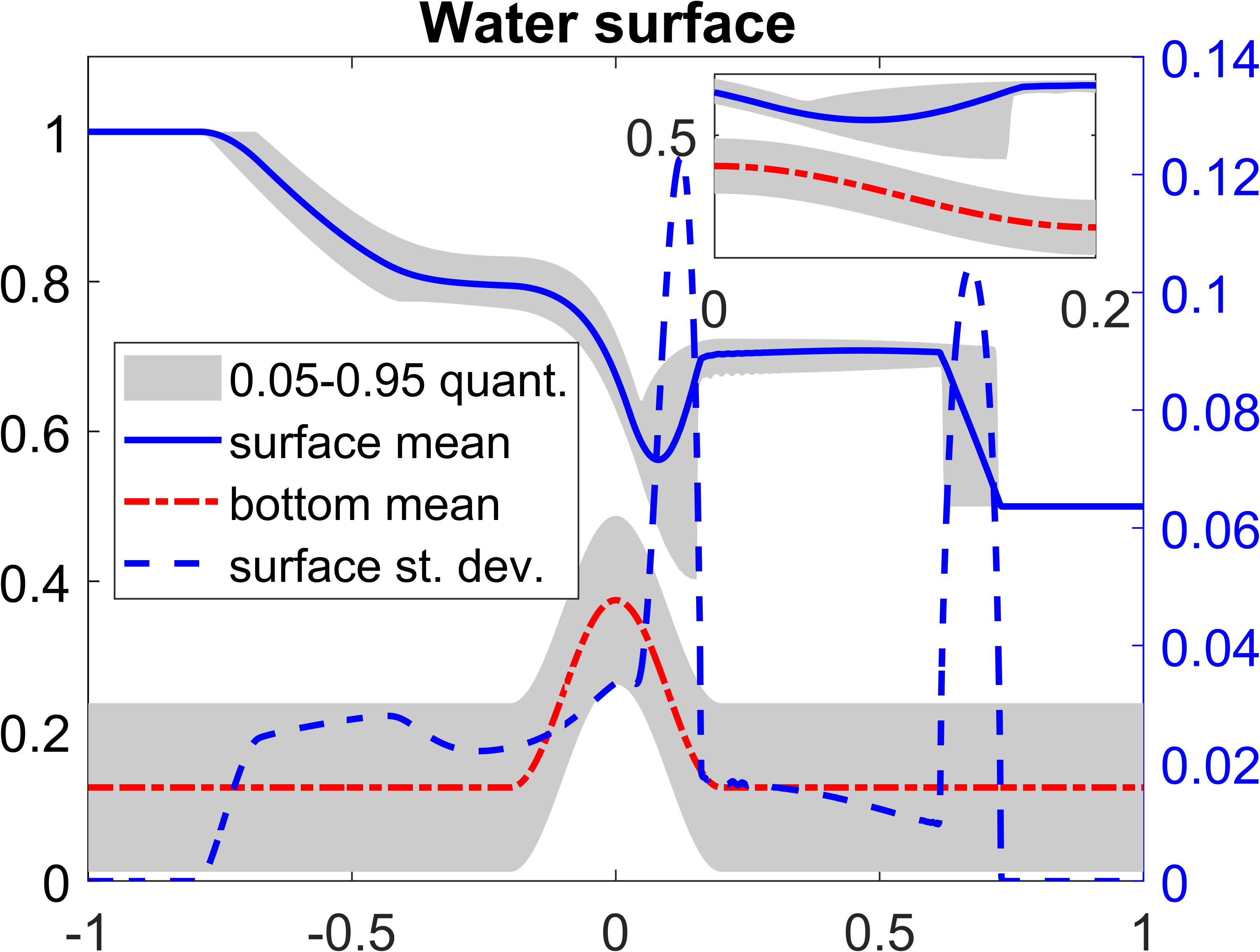
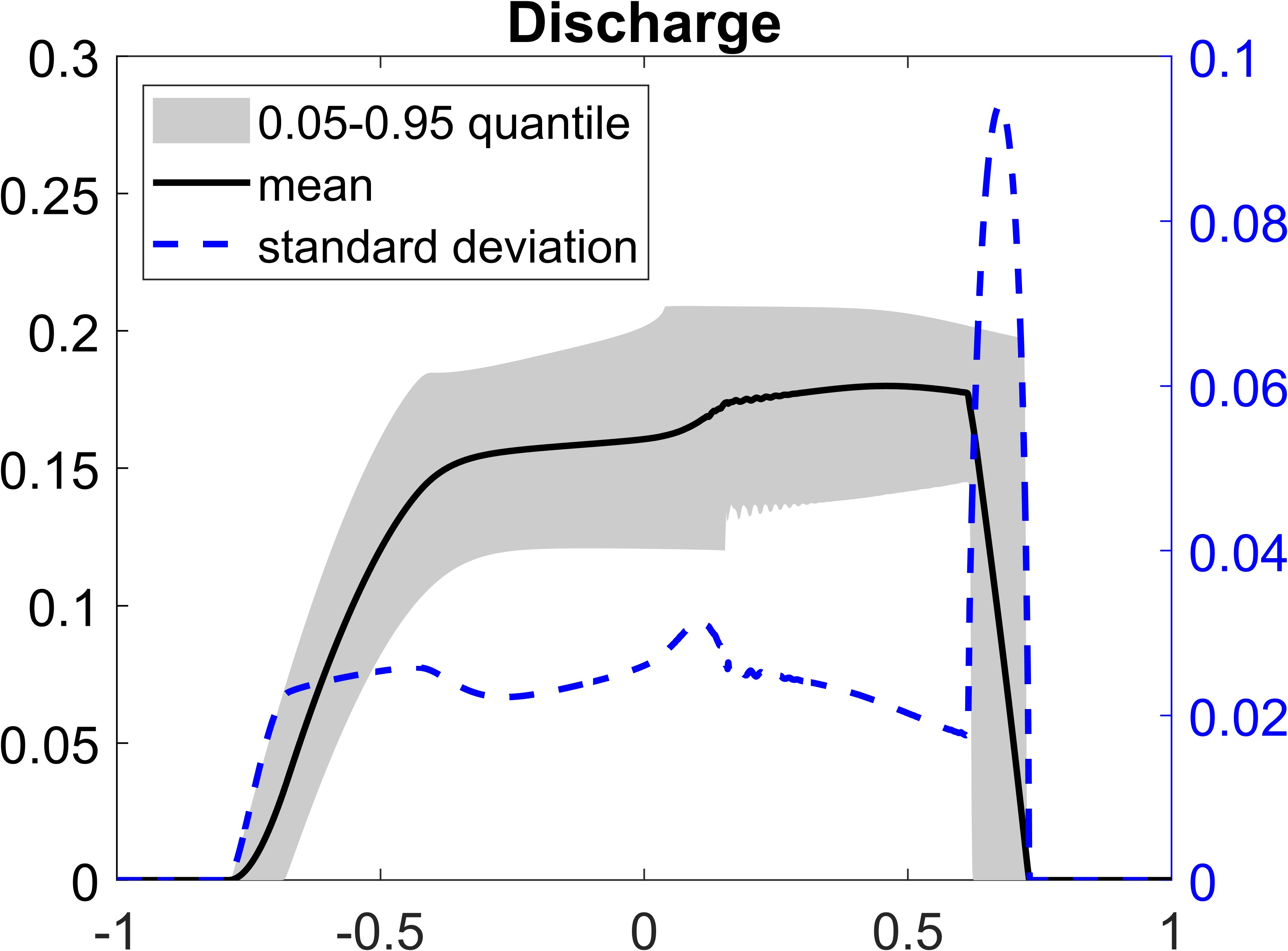
Figure 6.1: Example 5: Mean, 95%-quantile, and standard deviation of $w$ (left) and $hu$ (right).

Example 6 (Random Water Surface, $d=s=1$).

This example is taken from [7, Section 5.2]. We now consider the deterministic bottom topography

$$Z(x,\xi)=\left\{\begin{aligned} &10(x-0.3),&&0.3\leq x\leq 0.4,\\ &1-0.0025\sin^{2}(25\pi x),&&0.4\leq x\leq 0.6,\\ &-10(x-0.7),&&0.6\leq x\leq 0.7,\\ &0,&&\mbox{otherwise},\end{aligned}\right.$$

and the ICs with a randomly perturbed water surface

$$w(x,0,\xi)=\left\{\begin{aligned} &1.001+0.001\xi,&&0.1<x<0.2,\\ &1,&&\mbox{otherwise},\end{aligned}\right.\qquad u(x,0,\xi)\equiv 0.$$

The spatial domain is $x\in[-1,1]$ and free BCs are implemented at both ends of the interval. The water surface $w$ and discharge $hu$, computed on a uniform grid with $\Delta x=1/800$ and $\Delta\xi=1/50$ at time $t=1$ are plotted in Figure 6.2. The obtained results are similar to those obtained in [7] using a gPC-SG method, but our results are visibly sharper. We believe that the filter used in [7] causes additional smearing so that the main advantage of the gPC-SG method—spectral accuracy in the random space—is lost.

     

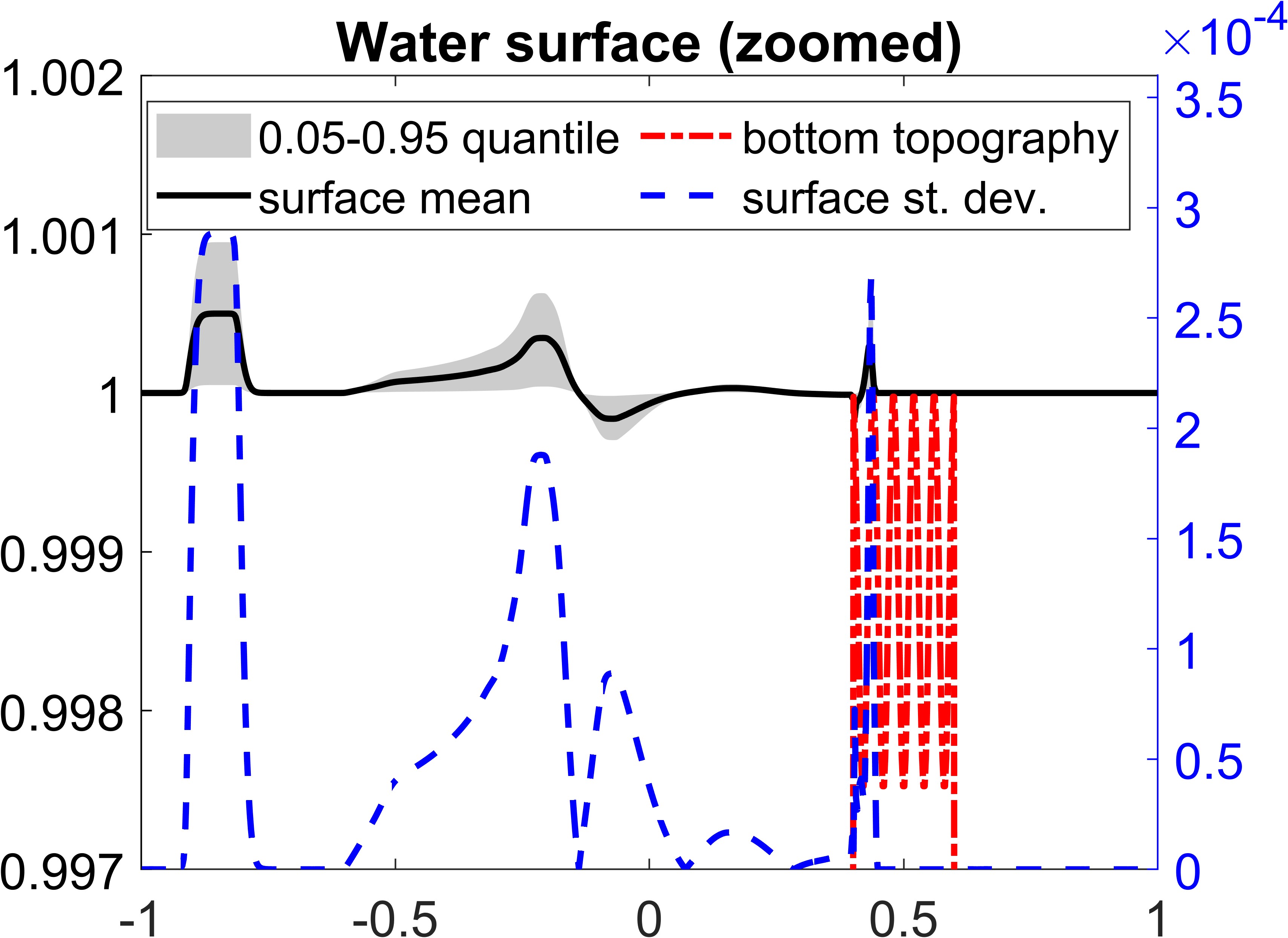
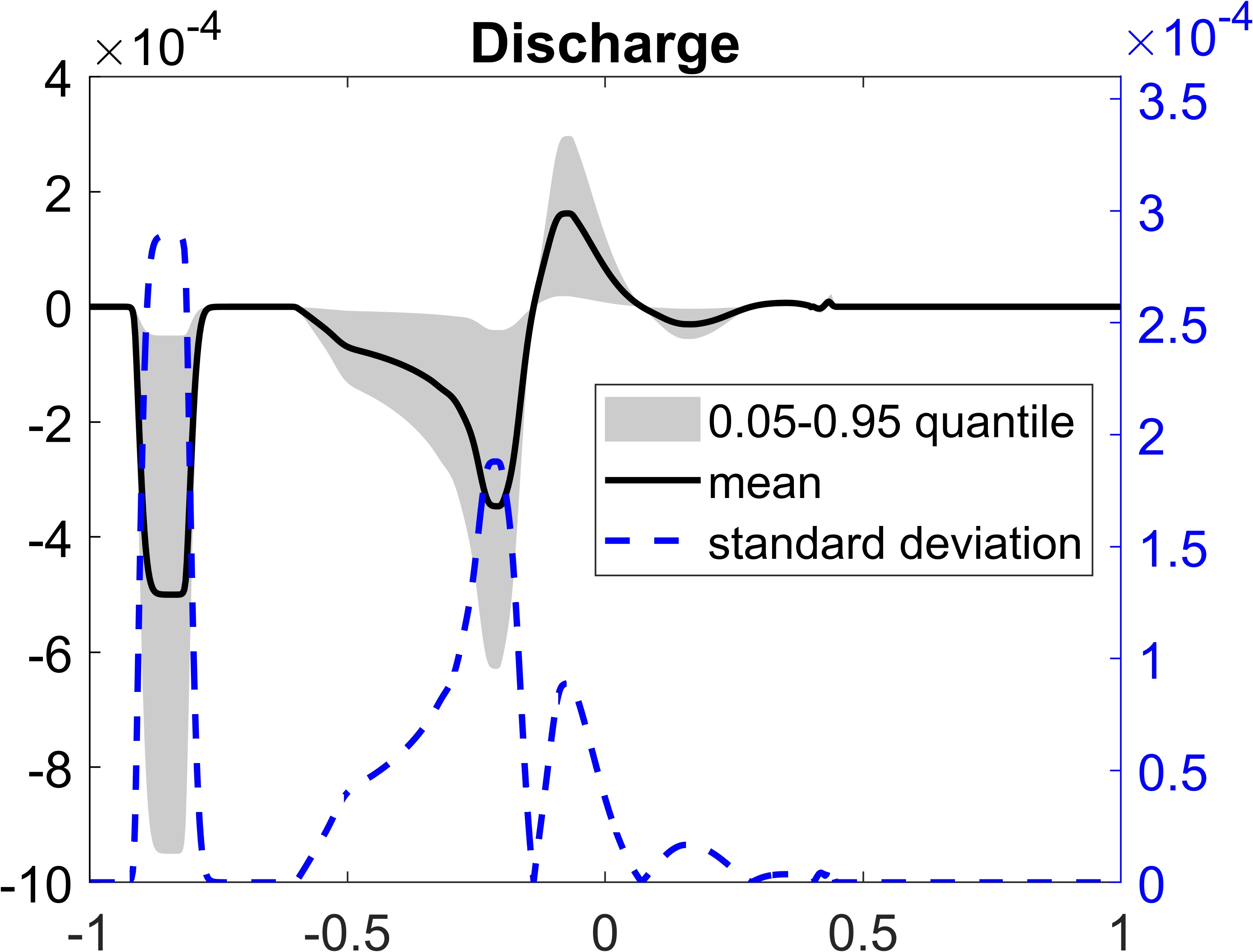
Figure 6.2: Example 6: Mean, 95%-quantile, and standard deviation of $w$ (left) and $hu$ (right).

Example 7 (Random Water Surface and Discharge, $d=1$, $s=2$).

We take random ICs for perturbed water surface and discharge,

$$w(x,\xi,\eta,0)=\max\big{\{}0.9,Z(x,\xi,\eta)\big{\}}+\left\{\begin{aligned} &0.1(1+0.1\xi),&&-1.6<x<-1.4,\\ &0,&&\text{otherwise},\end{aligned}\right.$$

$$u(x,\xi,\eta,0)=0.01\eta,$$

and the following deterministic bottom topography:

$$Z(x,\xi,\eta)=\left\{\begin{aligned} &(1-x^{2}),&&-1<x<1,\\ &0,&&\text{otherwise},\end{aligned}\right.$$

all considered in the spatial domain is $x\in[-4,2]$ with free BCs implemented at both ends of the interval.

In this example, the ICs give rise to two waves, which emerge in the area $x\in[-1.6,-1.4]$ and then propagate in the opposite directions. The right-moving wave reaches the initially dry area and then moves over the “island”, leading to the occurance of wetting/drying processes. This makes the studied problem numerically challenging. However, the proposed finite-volume method is capable of robustly capturing the solution as shown in Figure 6.3, where time snapshots of the mean and standard deviation of the water surface, computed on a uniform mesh with $\Delta x=1/100$ and $\Delta\xi=\Delta\eta=1/10$, are plotted.

     

     

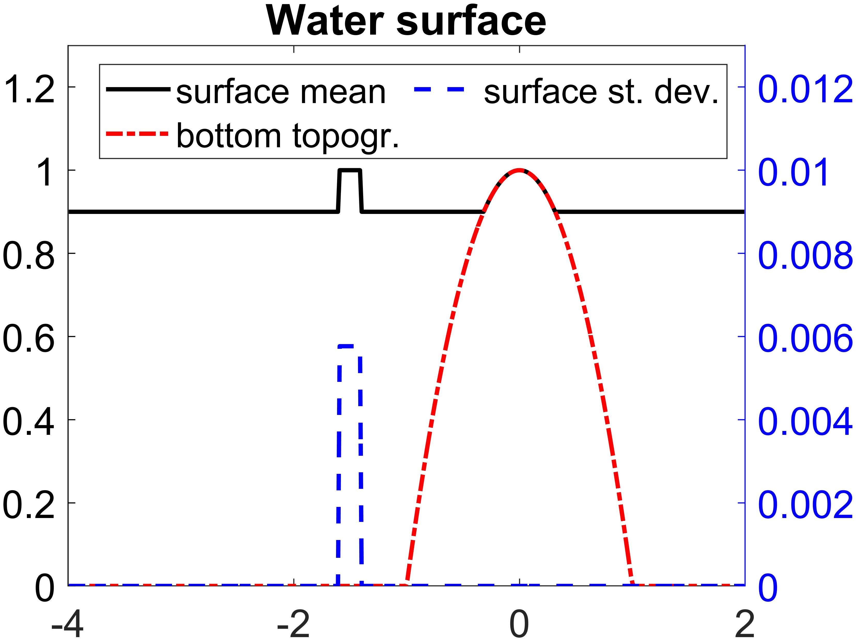
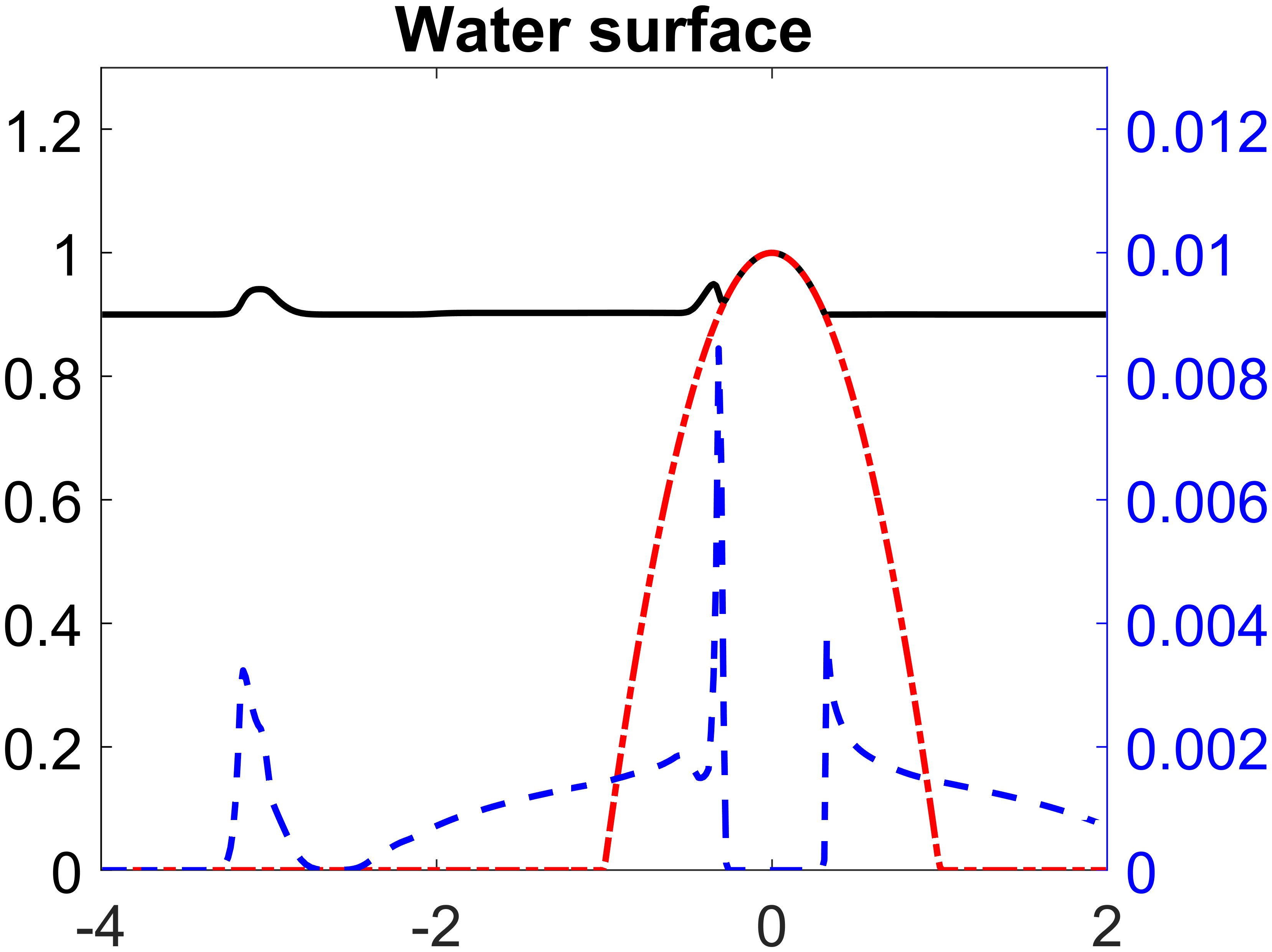
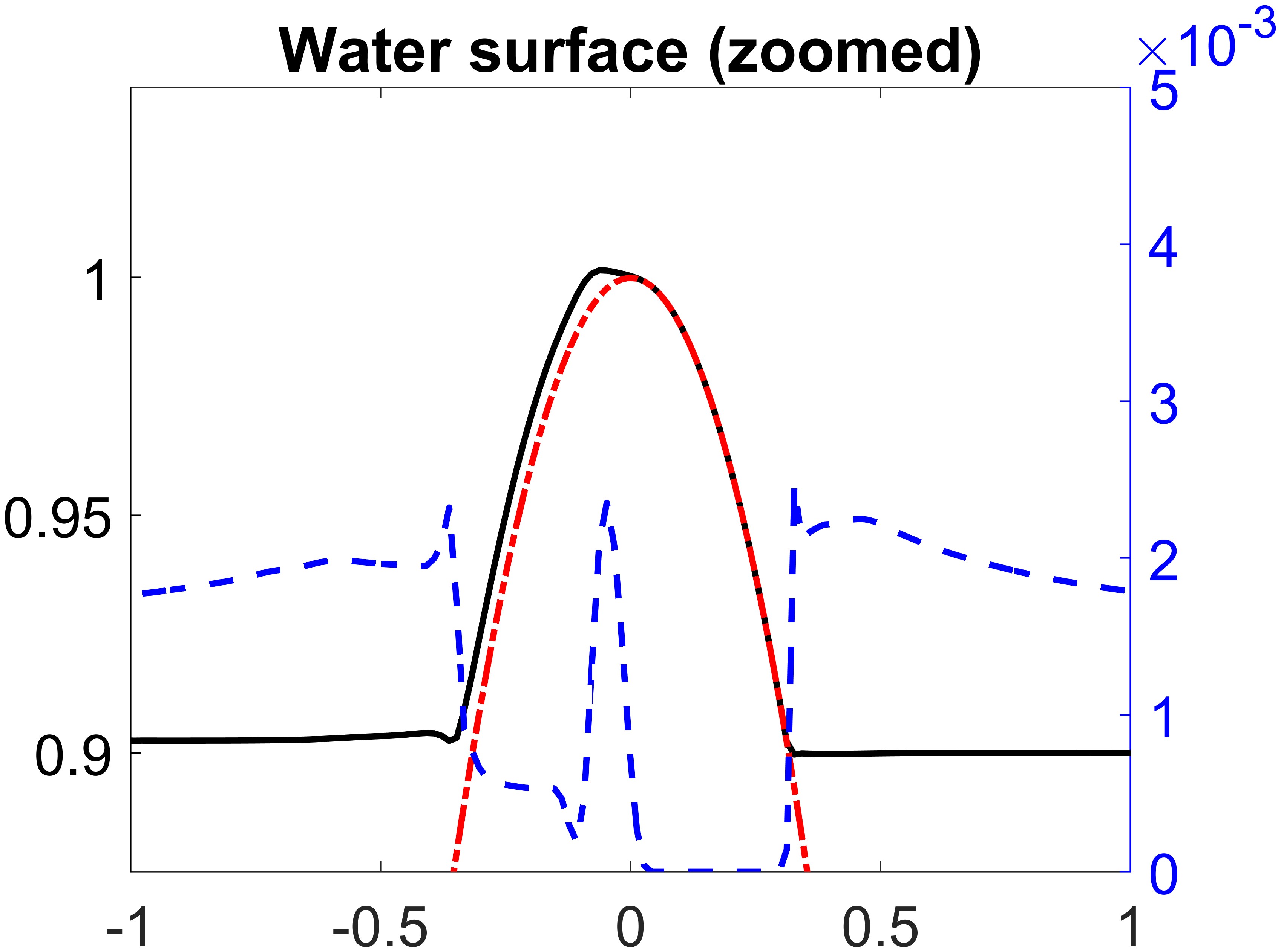
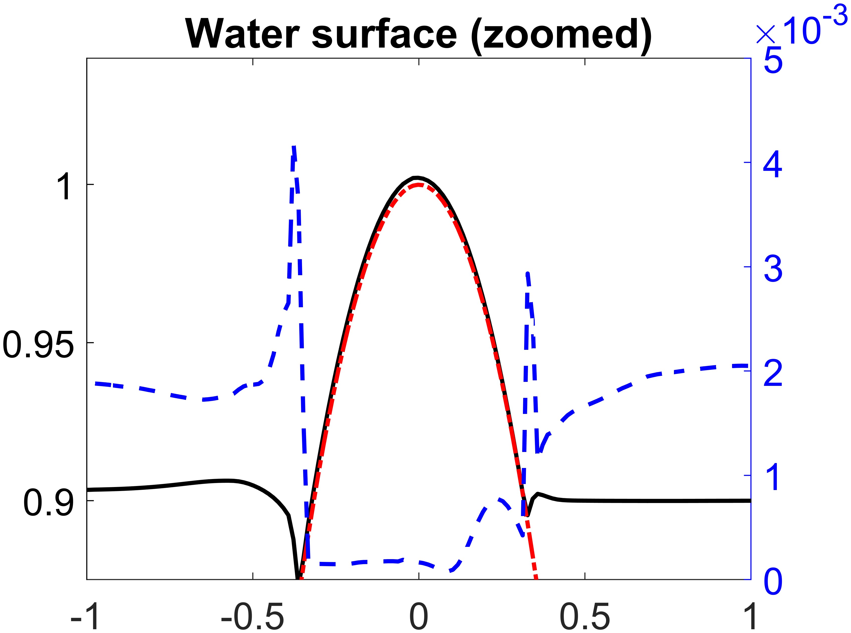
Figure 6.3: Example 7: Mean and standard deviation of $w$ at $t=0$ (top left), 0.5 (top right), 0.75 (bottom left), and 1 (bottom right).

Example 8 (Random Bottom Topography, $d=2$, $s=1$).

In the final example, we consider the deterministic ICs

$$w(x,y,\xi,0)=\left\{\begin{aligned} &\max\big{\{}1.01,Z(x,y)\big{\}},&&0.05<x<0.15,\\ &\max\big{\{}1,Z(x,y)\big{\}},&&\mbox{otherwise}\end{aligned}\right.\qquad u(x,y,\xi,0)\equiv 0,$$

and the following random bottom topography:

$$Z(x,y,\xi)=0.8e^{-5(x-0.9)^{2}-50(y-0.5)^{2}}+0.1(\xi+1),$$

in the spatial domain $(x,y)\in[0,2]\times[0,1]$ with free BCs prescribed at all sides of its boundary.

In Figure 6.4, we plot the mean and standard deviation of the water surface computed on a uniform mesh with $\Delta x=\Delta y=1/200$ and $\Delta\xi=1/10$ at time $t=1.2$. As in Example 3, the standard deviation identifies the areas in which the uncertainties the solution the most.

         

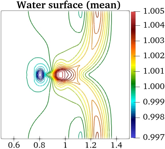
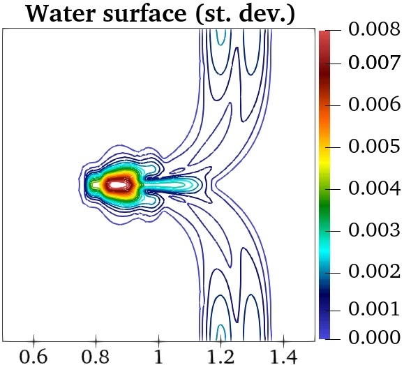
Figure 6.4: Example 8: Mean (left) and standard deviation (right) of $w$.

7 Conclusions

In this paper, we have introduced new well-balanced and positivity preserving finite-volume methods for nonlinear hyperbolic systems of PDEs with uncertainties. These methods are based on finite-volume approximation in both the spatial and random directions. In order to achieve a high order of accuracy, we have applied second-order minmod reconstruction in physical space and fifth-order Ai-WENO-Z interpolation in random directions. The lack of boundary conditions in the random space requires the development of a special high-order interpolation technique near the boundary. This has been achieved by designing a new one-sided Ai-WENO-Z interpolation. Even though, our numerical experiments did not show any sensitivity towards this choice, we note that it may possibly lead to instabilities if, for instance, strong discontinuities travel to a random boundary. We also note that the proposed high-order finite-volume method is well suited for hyperbolic systems with low or medium dimensional uncertainties. In order to overcome the curse of dimensionality, we suggest to apply GPU parallelization for high-dimensional random spaces. Both the problem of boundary conditions and curse of dimensionality in random space constitute interesting topics for future research.

Conflict of Interest Statement

On behalf of all authors, the corresponding author states that there is no conflict of interest.

Acknowledgment:

The work of A. Chertock was supported in part by NSF grant DMS-2208438. The work of M. Herty was supported in part by the DFG (German Research Foundation) through 20021702/GRK2326, 333849990/IRTG-2379, HE5386/ 18-1, 19-2, 22-1, 23-1, and under Germany’s Excellence Strategy EXC-2023 Internet of Production 390621612. The work of A. Kurganov was supported in part by NSFC grant 12171226 and the fund of the Guangdong Provincial Key Laboratory of Computational Science and Material Design (No. 2019B030301001). The work of M. Lukáčová-Medvid’ová has been funded by the DFG under the SFB/TRR 146 Multiscale Simulation Methods for Soft Matter Systems. M. Lukáčová-Medvid’ová gratefully acknowledges the support of the Gutenberg Research College of University Mainz and the Mainz Institute of Multiscale Modeling. M. Lukáčová-Medvid’ová and M. Herty also acknowledge the support of the DFG through the project 525853336 funded within the Focused Programme SPP 2410 “Hypebrolic Balance Laws: Complexity, Scales and Randomness”.

References

- [1] R. Abgrall and P. M. Congedo, A semi-intrusive deterministic approach to uncertainty quantification in non-linear fluid flow problems, J. Comput. Phys., 235 (2013), pp. 828–845.
- [2] R. Abgrall and S. Mishra, Uncertainty quantification for hyperbolic systems of conservation laws, in Handbook of numerical methods for hyperbolic problems, vol. 18 of Handb. Numer. Anal., Elsevier/North-Holland, Amsterdam, 2017, pp. 507–544.
- [3] R. Abgrall and S. Tokareva, The stochastic finite volume method, in Uncertainty quantification for hyperbolic and kinetic equations, vol. 14 of SEMA SIMAI Springer Ser., Springer, Cham, 2017, pp. 1–57.
- [4] T. Barth, Non-intrusive uncertainty propagation with error bounds for conservation laws containing discontinuities, in Uncertainty quantification in computational fluid dynamics, vol. 92 of Lect. Notes Comput. Sci. Eng., Springer, Heidelberg, 2013, pp. 1–57.
- [5] A. Bollermann, S. Noelle, and M. Lukáčová-Medviďová, Finite volume evolution Galerkin methods for the shallow water equations with dry beds, Commun. Comput. Phys., 10 (2011), pp. 371–404.
- [6] A. J. Chorin, Gaussian fields and random flow, J. Fluid Mech., 63 (1974), pp. 21–32.
- [7] D. Dai, Y. Epshteyn, and A. Narayan, Hyperbolicity-preserving and well-balanced stochastic Galerkin method for shallow water equations, SIAM J. Sci. Comput., 43 (2021), pp. A929–A952.
- [8] D. Dai, Y. Epshteyn, and A. Narayan, Hyperbolicity-preserving and well-balanced stochastic Galerkin method for two-dimensional shallow water equations, J. Comput. Phys., 452 (2022). Paper No. 110901, 28 pp.
- [9] B. Després, G. Poëtte, and D. Lucor, Robust uncertainty propagation in systems of conservation laws with the entropy closure method, in Uncertainty quantification in computational fluid dynamics, vol. 92 of Lect. Notes Comput. Sci. Eng., Springer, Heidelberg, 2013, pp. 105–149.
- [10] A. Ditkowski, G. Fibich, and A. Sagiv, Density estimation in uncertainty propagation problems using a surrogate model, SIAM/ASA J. Uncertain. Quantif., 8 (2020), pp. 261–300.
- [11] W. S. Don, D.-M. Li, Z. Gao, and B.-S. Wang, A characteristic-wise alternative WENO-Z finite difference scheme for solving the compressible multicomponent non-reactive flows in the overestimated quasi-conservative form, J. Sci. Comput., 82 (2020). Paper No. 27, 24 pp.
- [12] W. S. Don, R. Li, B.-S. Wang, and Y. H. Wang, A novel and robust scale-invariant WENO scheme for hyperbolic conservation laws, J. Comput. Phys., 448 (2022). Paper No. 110724, 23 pp.
- [13] J. Dürrwächter, T. Kuhn, F. Meyer, L. Schlachter, and F. Schneider, A hyperbolicity-preserving discontinuous stochastic Galerkin scheme for uncertain hyperbolic systems of equations, J. Comput. Appl. Math., 370 (2020). Paper No. 112602, 22 pp.
- [14] G. Geraci, P. M. Congedo, R. Abgrall, and G. Iaccarino, A novel weakly-intrusive non-linear multiresolution framework for uncertainty quantification in hyperbolic partial differential equations, J. Sci. Comput., 66 (2016), pp. 358–405.
- [15] S. Gerster and M. Herty, Entropies and symmetrization of hyperbolic stochastic Galerkin formulations, Commun. Comput. Phys., 27 (2020), pp. 639–671.
- [16] S. Gerster, M. Herty, and E. Iacomini, Stability analysis of a hyperbolic stochastic Galerkin formulation for the Aw-Rascle-Zhang model with relaxation, Math. Biosci. Eng., 18 (2021), pp. 4372–4389.
- [17] S. Gerster, M. Herty, and A. Sikstel, Hyperbolic stochastic Galerkin formulation for the -system, J. Comput. Phys., 395 (2019), pp. 186–204.
- [18] S. Gottlieb, D. Ketcheson, and C.-W. Shu, Strong stability preserving Runge-Kutta and multistep time discretizations, World Scientific Publishing Co. Pte. Ltd., Hackensack, NJ, 2011.
- [19] S. Gottlieb, C.-W. Shu, and E. Tadmor, Strong stability-preserving high-order time discretization methods, SIAM Rev., 43 (2001), pp. 89–112.
- [20] J. Jakeman, R. Archibald, and D. Xiu, Characterization of discontinuities in high-dimensional stochastic problems on adaptive sparse grids, J. Comput. Phys., 230 (2011), pp. 3977–3997.
- [21] Y. Jiang, C.-W. Shu, and M. Zhang, An alternative formulation of finite difference weighted ENO schemes with Lax-Wendroff time discretization for conservation laws, SIAM J. Sci. Comput., 35 (2013), pp. A1137–A1160.
- [22] S. Jin and R. Shu, A study of hyperbolicity of kinetic stochastic Galerkin system for the isentropic Euler equations with uncertainty, Chinese Ann. Math. Ser. B, 40 (2019), pp. 765–780.
- [23] A. Kurganov, S. Noelle, and G. Petrova, Semidiscrete central-upwind schemes for hyperbolic conservation laws and Hamilton-Jacobi equations, SIAM J. Sci. Comput., 23 (2001), pp. 707–740.
- [24] A. Kurganov and G. Petrova, A second-order well-balanced positivity preserving central-upwind scheme for the Saint-Venant system, Commun. Math. Sci., 5 (2007), pp. 133–160.
- [25] A. Kurganov and E. Tadmor, Solution of two-dimensional riemann problems for gas dynamics without Riemann problem solvers, Numer. Methods Partial Differential Equations, 18 (2002), pp. 584–608.
- [26] O. P. Le Maître and O. M. Knio, Spectral methods for uncertainty quantification, Scientific Computation, Springer, New York, 2010. With applications to computational fluid dynamics.
- [27] O. P. Le Maître, O. M. Knio, H. N. Najm, and R. G. Ghanem, Uncertainty propagation using Wiener-Haar expansions, J. Comput. Phys., 197 (2004), pp. 28–57.
- [28] P. Li, T. T. Li, W. S. Don, and B.-S. Wang, Scale-invariant multi-resolution alternative WENO scheme for the Euler equations, J. Sci. Comput., (2023). Paper No. 15, 32 pp.
- [29] K.-A. Lie and S. Noelle, On the artificial compression method for second-order nonoscillatory central difference schemes for systems of conservation laws, SIAM J. Sci. Comput., 24 (2003), pp. 1157–1174.
- [30] H. Liu, A numerical study of the performance of alternative weighted ENO methods based on various numerical fluxes for conservation law, Appl. Math. Comput., 296 (2017), pp. 182–197.
- [31] S. Mishra and C. Schwab, Sparse tensor multi-level Monte Carlo finite volume methods for hyperbolic conservation laws with random initial data, Math. Comp., 81 (2012), pp. 1979–2018.
- [32] S. Mishra and C. Schwab, Monte-Carlo finite-volume methods in uncertainty quantification for hyperbolic conservation laws, in Uncertainty quantification for hyperbolic and kinetic equations, vol. 14 of SEMA SIMAI Springer Ser., Springer, Cham, 2017, pp. 231–277.
- [33] S. Mishra, C. Schwab, and J. Šukys, Multi-level Monte Carlo finite volume methods for nonlinear systems of conservation laws in multi-dimensions, J. Comput. Phys., 231 (2012), pp. 3365–3388.
- [34] S. Mishra, C. Schwab, and J. Šukys, Multilevel Monte Carlo finite volume methods for shallow water equations with uncertain topography in multi-dimensions, SIAM J. Sci. Comput., 34 (2012), pp. B761–B784.
- [35] S. Mishra, C. Schwab, and J. Šukys, Multi-level Monte Carlo finite volume methods for uncertainty quantification in nonlinear systems of balance laws, in Uncertainty quantification in computational fluid dynamics, vol. 92 of Lect. Notes Comput. Sci. Eng., Springer, Heidelberg, 2013, pp. 225–294.
- [36] H. Nessyahu and E. Tadmor, Nonoscillatory central differencing for hyperbolic conservation laws, J. Comput. Phys., 87 (1990), pp. 408–463.
- [37] M. Petrella, S. Tokareva, and E. F. Toro, Uncertainty quantification methodology for hyperbolic systems with application to blood flow in arteries, J. Comput. Phys., 386 (2019), pp. 405–427.
- [38] M. P. Pettersson, G. Iaccarino, and J. Nordström, Polynomial chaos methods for hyperbolic partial differential equations, Mathematical Engineering, Springer, Cham, 2015. Numerical techniques for fluid dynamics problems in the presence of uncertainties.
- [39] P. Pettersson, G. Iaccarino, and J. Nordström, A stochastic Galerkin method for the Euler equations with Roe variable transformation, J. Comput. Phys., 257 (2014), pp. 481–500.
- [40] G. Poëtte, B. Després, and D. Lucor, Uncertainty quantification for systems of conservation laws, J. Comput. Phys., 228 (2009), pp. 2443–2467.
- [41] L. Schlachter and F. Schneider, A hyperbolicity-preserving stochastic Galerkin approximation for uncertain hyperbolic systems of equations, J. Comput. Phys., 375 (2018), pp. 80–98.
- [42] J. Shi, C. Hu, and C.-W. Shu, A technique of treating negative weights in WENO schemes, J. Comput. Phys., 175 (2002), pp. 108–127.
- [43] J. Šukys, S. Mishra, and C. Schwab, Multi-level Monte Carlo finite difference and finite volume methods for stochastic linear hyperbolic systems, in Monte Carlo and quasi-Monte Carlo methods 2012, vol. 65 of Springer Proc. Math. Stat., Springer, Heidelberg, 2013, pp. 649–666.
- [44] P. K. Sweby, High resolution schemes using flux limiters for hyperbolic conservation laws, SIAM J. Numer. Anal., 21 (1984), pp. 995–1011.
- [45] T. Tang and T. Zhou, Convergence analysis for stochastic collocation methods to scalar hyperbolic equations with a random wave speed, Commun. Comput. Phys., 8 (2010), pp. 226–248.
- [46] S. Tokareva, A. Zlotnik, and V. Gyrya, Stochastic finite volume method for uncertainty quantification of transient flow in gas pipeline networks, Appl. Math. Model., 125 (2024), pp. 66–84.
- [47] J. Tryoen, O. Le Maître, M. Ndjinga, and A. Ern, Intrusive Galerkin methods with upwinding for uncertain nonlinear hyperbolic systems, J. Comput. Phys., 229 (2010), pp. 6485–6511.
- [48] J. Tryoen, O. Le Maitre, M. Ndjinga, and A. Ern, Roe solver with entropy corrector for uncertain hyperbolic systems, J. Comput. Appl. Math., 235 (2010), pp. 491–506.
- [49] X. Wan and G. E. Karniadakis, Multi-element generalized polynomial chaos for arbitrary probability measures, SIAM J. Sci. Comput., 28 (2006), pp. 901–928.
- [50] B.-S. Wang and W. S. Don, Affine-invariant WENO weights and operator, Appl. Numer. Math., 181 (2022), pp. 630–646.
- [51] B.-S. Wang, P. Li, Z. Gao, and W. S. Don, An improved fifth order alternative WENO-Z finite difference scheme for hyperbolic conservation laws, J. Comput. Phys., 374 (2018), pp. 469–477.
- [52] K. Wu, H. Tang, and D. Xiu, A stochastic Galerkin method for first-order quasilinear hyperbolic systems with uncertainty, J. Comput. Phys., 345 (2017), pp. 224–244.
- [53] K. Wu, D. Xiu, and X. Zhong, A WENO-based stochastic Galerkin scheme for ideal MHD equations with random inputs, Commun. Comput. Phys., 30 (2021), pp. 423–447.
- [54] D. Xiu, Efficient collocational approach for parametric uncertainty analysis, Commun. Comput. Phys., 2 (2007), pp. 293–309.
- [55] D. Xiu, Fast numerical methods for stochastic computations: a review, Commun. Comput. Phys., 5 (2009), pp. 242–272.
- [56] D. Xiu, Numerical methods for stochastic computations, Princeton University Press, Princeton, NJ, 2010. A spectral method approach.
- [57] X. Zhong and C.-W. Shu, Entropy stable Galerkin methods with suitable quadrature rules for hyperbolic systems with random inputs, J. Sci. Comput., 92 (2022). Paper No. 14, 30 pp.