Energy spectra of elemental groups of cosmic rays with the KASCADE experiment data and machine learning

Abstract

We report the reconstruction of the mass component spectra of cosmic rays (protons, helium, carbon, silicon, and iron) and their mean mass composition, at energies from 1.4 to 100 PeV. The results are derived from the archival data of the extensive air shower experiment KASCADE. We use a novel machine learning technique, developed specifically for this reconstruction, and modern hadronic interaction models: QGSJet.II-04, EPOS-LHC and Sibyll 2.3c. We have found a marked excess of the proton component and deficit of intermediate and heavy nuclei components, compared to the original KASCADE results. At the same time our results are partially consistent with the results of IceTop and TALE experiments. The systematic uncertainties are computed taking into account the difference between the hadronic models and have a similar magnitude as the uncertainties of other mentioned experiments, that were computed without cross-hadronic model systematics.

1 Introduction

Measurements of the cosmic-ray energy spectrum and the separate mass component spectra in the 1 to 100 PeV energy range provide important information for understanding the sources, acceleration, and propagation mechanisms of galactic cosmic rays (CRs). They are also essential in searching for the energy region where the transition from galactic to extragalactic CRs takes place. In particular, many mechanisms of the CR acceleration naturally predict that the maximum energy achievable by cosmic rays is proportional to their charge. This should lead to the sequence of steepenings in the spectra of CR mass components related to the end of their injected spectra in galactic sources [1].

A first indication that such behavior of CR component spectra is indeed taking place was found by the KASCADE experiment [2]. Although the increase of the mean mass of the CR flux with energy was supported by other experiments in general, there is a controversy about the particular proportion of separate mass components in the flux depending on energy. The study of CRs with energies above $\sim 1$ PeV is complicated as one can only observe it indirectly through extensive air showers (EAS) of secondary particles that they initiate in the Earth’s atmosphere. Therefore, the results of various experiments are subject to a number of systematic uncertainties accompanying the reconstruction of primary particle features from the EAS observables. In addition to the original KASCADE mass component results [2, 3, 4] we can mention studies of other experiments: CASA-BLANCA [5], Tibet AS$\gamma$ [6], KASCADE-Grande [4, 7], Tunka-133 [8], IceTop [9] and TALE [10], in the energy range of interest.

In this research, we present mass component spectra reconstruction with machine learning methods using archival data from the KASCADE experiment [11], provided by the KASCADE Cosmic Ray Data Centre (KCDC) [12]. In the original KASCADE analyses [2, 3, 4, 13], the method of two-dimensional unfolding was used, in which a distribution of events over the reconstructed numbers of electrons and muons was converted into a distribution over the type and energy of the primary particle. In this research, we use a different approach to reanalyze the original data of the KASCADE experiment and to re-derive the CR mass component spectra from it. This approach combines the event-by-event classification of the primary particle type with machine learning [14, 15, 16] and two separate unfolding procedures for the correction of the reconstructed primary particle type and energy [16]. An additional feature of our analysis is the incorporation of the difference between three modern hadronic interaction models (QGSJet-II.04 [17], EPOS-LHC [18] and Sibyll 2.3c [19]) into a total systematic uncertainty. A detailed description of our methods and their uncertainties was given in Ref. [16].

The paper is organized as follows: in Section 2, we briefly describe the data and Monte Carlo (MC) that we are using. Section 3 outlines the main details of our analysis and also describes some features that were not presented in our methodological paper [16]. Namely, we discuss the computation of the cross-hadronic model uncertainty and the method of the mean logarithmic mass reconstruction. In Section 4, we show the main results of this study: the reconstructed spectra of separate mass components and the mean logarithmic mass. We also compare these results with other experiments. The discussion and conclusion are presented in Section 5.

2 Experiment, data and Monte Carlo

In this study, we analyze the archival data of the KASCADE experiment using the machine learning methods developed specifically for this task. The KASCADE air shower experiment was operated from 1996 to 2013 at the KIT Campus in Karlsruhe, Germany (${49.1}^{\circ}$ north, ${8.4}^{\circ}$ east at 110 m a.s.l). This experiment studied extensive air showers in the primary energy range from $\sim 500$ TeV to 100 PeV. The experiment collected data from different setups, but in this research, we use the data from the main KASCADE array only. This array was composed of 252 scintillator detectors placed in the rectangular grid covering the $200\times 200$ m² area. Outer detectors contain a shielding layer to detect electromagnetic and muon-dominated EAS parts separately.

The experimental and Monte Carlo data we are using in this study were provided by KCDC service [12]. Each event includes time-integrated deposits of electromagnetic and muon EAS components from the KASCADE array stations, as well as reconstructed features: primary energy ($E$), zenith angle ($\theta$), azimuthal angle ($\phi$), shower core position ($x$, $y$), number of electrons ($N_{e}$) and muons ($N_{\mu}$), and shower age ($s$). The values $N_{e}$, $N_{\mu}$, and $s$ are determined by fitting the lateral distribution function of the event with the modified NKG function [20]. $E$ is reconstructed with the standard KASCADE algorithms by taking into account both $N_{e}$ and $N_{\mu}$ corrected for atmospheric attenuation depending on $\theta$, see Ref. [20] for more details. The resolution of $E$ is around $11\%$ in terms of the decimal logarithm of the ratio of the simulated to the reconstructed energies for MC events based on the QGSJet.II-04 hadronic interaction model, which passed the quality cuts in the studied energy range (see below) .

The full efficiency of the trigger and reconstruction is reached at $E>10^{15}$ eV. We use the quality cuts recommended by KASCADE [2]: ${\theta<18^{\circ}}$, ${\sqrt{x^{2}+y^{2}}<91}$ m, ${\log_{10}N_{e}>4.8}$, ${\log_{10}N_{\mu}>3.6}$, and the cut on the shower age set by KCDC: ${0.2<s<1.48}$ [20], which is stricter than the original one (${0.2<s<2.1}$). We also impose the additional cut on the reconstructed event energy $E>10^{15.15}$ eV to ensure the stability of the unfolding procedure.

Overall, we have $\sim 3.5\cdot 10^{6}$ experimental events in the studied energy range that passed the quality cuts. The entire experimental dataset was divided into the so-called “blind” and “unblind” parts in an 80:20 ratio by random partitioning. The “unblind” part was used to check the correctness of the applied methods in our study [16]. The results for the “blind” part are disclosed in this paper. Also, we use a number of MC datasets simulated with CORSIKA [22] for three different modern hadronic interaction models: QGSJet-II.04 [17], EPOS-LHC [18] and Sibyll 2.3c [19], provided by KCDC. For low-energy hadronic interactions ($E<200$ GeV), the FLUKA [23] model has been used. We have a total of $\sim 1.3\cdot 10^{5}$, $6.7\cdot 10^{4}$, and $6.8\cdot 10^{4}$ events that have passed the quality cuts in the studied energy range for QGSJet-II.04, EPOS-LHC and Sibyll 2.3c models respectively. These MC sets include simulations for five primary particle types: protons (p), helium (He), carbon (C), silicon (Si) and iron (Fe). In Ref. [16], we used MC based on the QGSJet.II-04 hadronic interaction model as a baseline, in line with the original KASCADE research [4] based on the QGSJet.II-02 [21] model. The results for EPOS-LHC and Sibyll 2.3c are used for a calculation of the total systematic uncertainty.

3 Method and uncertainties

All details of our methods and their application are available in our methodological paper [16]. In summary, we built a number of machine learning models to classify primary CRs into five groups: p, He, C, Si and Fe, on an event-by-event basis. Namely, a random forest (RF) classifier [24], a convolutional neural network (CNN) inspired by the LeNet-5 [25] architecture, a multi-layer perceptron and EfficientNetv2 [26] were constructed. The models were implemented with PyTorch [27], TensorFlow [28] and Scikit-learn [29] packages. The performance of these models was compared using their confusion matrices. This matrix represents the fraction of particles of each type that the given model classifies as this type (i.e., correctly) and all other types (i.e., incorrectly). The performance of the different classifiers was almost similar; we selected the CNN for further use because of its robustness demonstrated in various other tests performed in our methodological paper [16]. The CNN uses electromagnetic and muon deposits, $\theta$, $N_{e}$, $N_{\mu}$ and $s$ as input parameters. The example of the CNN confusion matrix for different energy intervals is shown in Fig. 1.

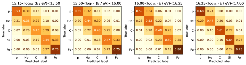
Figure 1: Confusion matrices of the CNN for the different reconstructed energy intervals. The neural network is trained and tested using the QGSJet-II.04 hadronic interaction model.

In Ref. [16], we used the CNN to reconstruct the mass component spectra of CRs in the “unblind” part of the experimental data. We enhanced the quality of mass component spectra reconstruction by performing the unfolding of our results with response matrices (that are transposed confusion matrices) derived from the MC simulations. We sequentially unfold the primary energy and primary particle type using the Bayesian iterative unfolding procedure [30] with pyunfold [31] python package. In that study, all uncertainties related to particle type and energy reconstruction, as well as uncertainties of the unfolding procedure, were estimated using the MC set with QGSJet.II-02 hadronic model and “unblind” data set. In what follows, we call these uncertainties “basic” ones. The results were shown to have better accuracy than that of the original KASCADE analysis [4].

In the present study, we apply the same analysis pipeline to the undisclosed portion (“blind” part) of the experimental data. We re-compute all the basic uncertainties using the MC set based on the QGSJet.II-04 hadronic model and the “blind” data set. Namely, the computed uncertainties are: effect of “missing” detectors in experimental data (5 – 18 %, with respect to the reconstructed CR flux value), limited size of MC set (8 – 25 %), detection efficiency (up to $11\%$), energy resolution for different MC mixtures (13 – 16 %), spectral index in the MC set (up to $4\%$). Another set of systematic biases comes from sequential energy and particle type unfoldings (up to $8\%$) and the unfolding procedure itself (1 – 24 %). All the uncertainty estimates shown in brackets above have been calculated as an average overall mass component for the studied energy range after the full unfolding. The estimates for two other hadronic models considered in this study are quite similar (excluding outliers for EPOS-LHC, see below). We calculated the total basic systematic uncertainty (except cross-hadronic uncertainty, discussed below) as the square root of the sum of the squares of the uncertainties and biases described above, conservatively considering that they are independent.

In this study, we also consider the uncertainty originating from the use of three different hadronic interaction models: QGSJet.II-04, EPOS-LHC, and Sibyll 2.3c. We call this a cross-hadronic uncertainty. Also, we present our results for the mean logarithmic mass ($\left<\ln{A}\right>$) of the CR flux, depending on the primary energy. We discuss the computation of these quantities below.

Cross-hadronic model uncertainty.

To consider systematic uncertainties associated with a difference between hadronic interaction models, we first perform the unfolding procedures for each model and compute the respective systematic uncertainty band. This implies unfolding with the response matrices derived from the corresponding MC set for our CNN. As it was mentioned, we set the results obtained for QGSJet.II-04 model as our baseline, following the usage of the previous version of this model (QGSJet.II-02) in the original KASCADE mass composition study [4]. It also appears that the results for QGSJet.II-04 model are intermediate among two other models. For each mass component spectrum in each energy bin, we define the total systematic uncertainty, including the cross-hadronic one, simply as a range between the minimum and the maximum edges of the uncertainty bands among all the hadronic models used.

Mean logarithmic mass representation.

The results of several other experiments on the CR mass composition were presented in the form of $\left<\ln{A}\right>$ depending on the energy [9, 10]. Therefore, to make a reasonable comparison, we compute this quantity in the present paper too. We derive $\left<\ln{A}\right>$ by taking the weighted sum of the fluxes from the mass component spectra in each energy bin. To estimate the total systematic uncertainty for $\left<\ln{A}\right>$ (except the cross-hadronic one), we first calculate each uncertainty contribution of those discussed above separately. Each contribution is calculated using the propagation of uncertainty method. The contributions of the unfolding biases are calculated as the direct weighted sum of the biases. For the total basic uncertainty (except the cross-hadronic one), we combine all the contributions in quadrature, considering them to be uncorrelated. To account for the cross-hadronic uncertainty, we calculate $\left<\ln{A}\right>$ for all of our hadronic interaction models. By analogy, we take the QGSJet.II-04 results as a baseline and define the total uncertainty as a range between the lowest and highest edges of the uncertainty bands among all the hadronic models used.

4 Results

In this section, we show the energy spectra for elementary groups of cosmic rays obtained with the “blind” part of the KASCADE experimental data. The spectra reconstructed using QGSJet.II-04 hadronic interaction model are presented in Fig. 2.

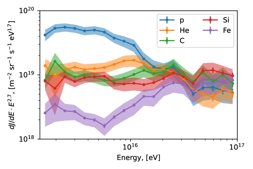
Figure 2: Mass component spectra reconstructed with our CNN method for the “blind” part of the experimental data using QGSJet-II.04 hadronic interaction model. Whiskers display the statistical uncertainties, while bands represent the systematic uncertainties.

Here, we include all the basic uncertainties described in Section 3 except the cross-hadronic uncertainty, they have value in a range 19 – 42 % depending on the energy when averaged over all mass components. For comparison, we can estimate the contribution of the cross-hadronic uncertainties (not shown in Fig. 2) alone. If we would define it as a range of the relative differences between the central values of the flux based on the QGSJet.II-04 hadronic interaction model and two other models, we would get a range of 4 – 48 % depending on the energy when averaged over all mass components. However, we need to stress that this estimation is only approximate since our definition of the total uncertainty given in the previous Section implies the inseparability of basic and cross-hadronic uncertainties.

The comparison between the original KASCADE mass component spectra (determined using QGSJet.II-02 hadronic model) and our final CNN results, including cross-hadronic uncertainties, is shown in Fig. 3.

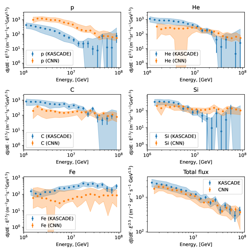
Figure 3: Comparison of the mass components spectra and all-particle spectra (right bottom) of the original KASCADE analysis [4], obtained for the QGSJet-II.02 hadronic interaction model (in blue) and our CNN analysis for the “blind” part of the experimental data, including cross-hadronic uncertainties (in orange). Whiskers display the statistical uncertainties, while bands represent the systematic uncertainties.

One can see that the total flux is in agreement, within uncertainties, for the original KASCADE and our CNN results. The statistical uncertainties of the KASCADE spectra exceed those of the CNN because the experimental dataset provided by KCDC that we use in this study is larger by a factor of about nine, compared to the dataset used in the KASCADE study [4]. At the same time, the uncertainties are dominated by systematic ones for almost all mass components at all energies for both analyses. Another point is that even when cross-hadronic uncertainties are taken into account for our CNN analysis, the widths of the total uncertainty bands are mostly comparable with those of the KASCADE result, where the cross-hadronic uncertainties are not included. However, our analysis yields a set of points (for He and Fe) with exceptionally wide bands. This effect is entirely due to the estimation of the unfolding bias uncertainty for the EPOS-LHC hadronic model results. In any case, the most pronounced discrepancy between the original KASCADE and the CNN results is the excess of the p component at low and intermediate energies in the latter.

We also compare our final CNN mass component spectra with the IceTop results [9] in Fig. 4. Note that IceTop results are obtained using the Sibyll 2.1 [32] hadronic interaction model and do not include cross-hadronic systematics. They also consider four different mass components: p, He, O, and Fe, instead of the five components considered in our analysis. Therefore, the comparison is not ideal, but in general, one can see the agreement between these results, taking into account the uncertainties.

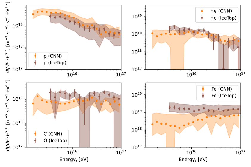
Figure 4: Comparison of the mass component spectra of IceTop [9] obtained for the Sibyll 2.1 hadronic interaction model (in brown) and our CNN spectra for the “blind” part of the experimental data, including cross-hadronic uncertainties (in orange). Whiskers display the statistical uncertainties, while bands represent the systematic uncertainties.

Finally, the comparison of results of our CNN method, IceTop [9] and TALE [10] in terms of $\left<\ln{A}\right>$ is shown in Fig. 5. For our method, $\left<\ln{A}\right>$ is calculated according to Section 3. Our result includes the cross-hadronic uncertainties, while the IceTop and TALE results are based on Sibyll 2.1 and EPOS-LHC hadronic interaction models, respectively, and do not include cross-hadronic uncertainties. The numerical tables of our results are presented in Appendix A.

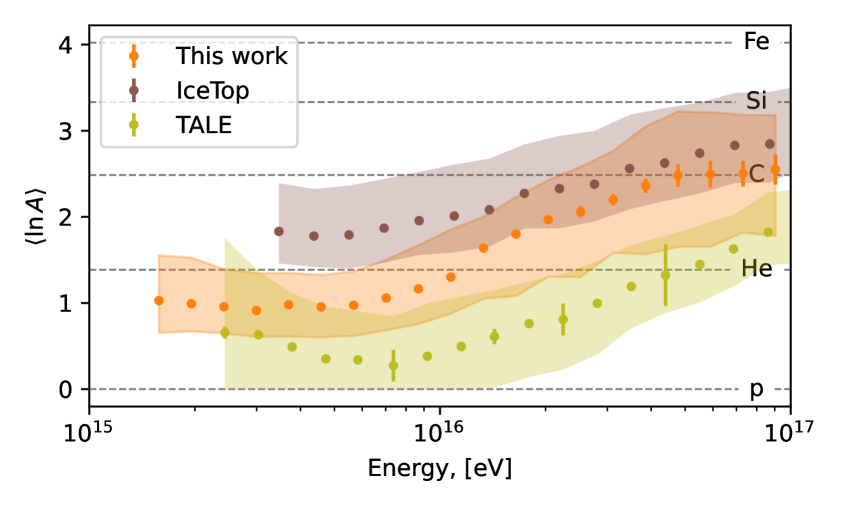
Figure 5: Comparison of the mean logarithmic mass ($\left<\ln{A}\right>$) of IceTop [9] obtained for the Sibyll 2.1 hadronic interaction model (in brown), TALE [10] obtained for the EPOS-LHC model (in green) and our CNN method for the “blind” part of the experimental data, including cross-hadronic uncertainties (in orange). Whiskers display the statistical uncertainties, while bands represent the systematic uncertainties.

5 Discussion and conclusion

In this research, we have presented the mass component spectra reconstructed with the specific convolutional neural network method using the KASCADE experiment archival data. We have performed the full unfolding analysis and computed all the uncertainties affecting the reconstruction and unfolding procedures. We also have taken into account the systematic uncertainty arising due to a difference between modern hadronic interaction models: QGSJet.II-04, EPOS-LHC and Sibyll 2.3c. We also compared our mass component spectra with the original KASCADE results [4] and with IceTop results [9]. Our all-particle spectrum is consistent with the original KASCADE one. Still, we observed a significant excess with respect to their proton component spectrum, for example, by a factor of $\sim 10$ at $E=10^{16}$ eV. At the same time, the mass component spectra are mostly in agreement with that of IceTop. We also converted our results to a form of $\left<\ln{A}\right>$ and compared it with those obtained by IceTop [9] and TALE [10]. One can see that our CNN results are generally in agreement with IceTop and TALE results within the systematic uncertainties. While the results of the two latter experiments do not agree with each other. We need to note that the total uncertainties of our results, which include the cross-hadronic models’ uncertainty, have the same order of magnitude as the IceTop and TALE results, which do not include such uncertainty.

As a result of this research, we realize that the systematic uncertainties can be further reduced by generating additional MC, which was a constraining factor for the present analysis. But, in any case, even a perfect particle type classification method would reduce the systematic uncertainties (for $\left<\ln{A}\right>$) from the current 22 – 53 % to 5 – 35 %, depending on the primary energy, if only the cross-hadronic uncertainties would be taken into account.

Appendix A Table of results

The values of $\left<\ln{A}\right>$ for our CNN reconstruction shown in Fig. 5 are represented in Table 1. The separate mass components spectra and the all-particle spectrum shown in Fig. 3 are represented in Table 2 and Table 3, respectively.

Table 1: $\left<\ln{A}\right>$ values for our CNN reconstruction. “Stat” means statistical uncertainties. “Sys.” means the total systematic uncertainties (including cross-hadronic uncertainty), “$+$“ is the upper edge of uncertainty, “$-$“ is the lower edge of uncertainty.

$\log_{10}(E/\text{eV})$	$\left<\ln{A}\right>$	Stat	$+$ Sys. $-$
15.196	1.028	0.007	0.525	0.375
15.289	0.992	0.013	0.534	0.320
15.382	0.957	0.011	0.437	0.311
15.474	0.914	0.011	0.431	0.305
15.566	0.980	0.013	0.369	0.370
15.659	0.955	0.015	0.372	0.351
15.752	0.973	0.017	0.394	0.355
15.844	1.059	0.020	0.443	0.376
15.936	1.165	0.023	0.506	0.408
16.029	1.302	0.027	0.550	0.426
16.121	1.638	0.026	0.364	0.589
16.214	1.800	0.034	0.427	0.719
16.306	1.967	0.038	0.459	0.662
16.398	2.058	0.065	0.522	0.757
16.492	2.199	0.064	0.568	0.615
16.584	2.361	0.082	0.688	0.795
16.676	2.481	0.131	0.741	0.831
16.769	2.495	0.155	0.719	0.840
16.861	2.502	0.148	0.682	0.683
16.954	2.549	0.174	0.632	0.771

Table 2: Separate mass components spectra in form $dJ/dE\cdot E^{2.5}$, $\left[\text{m}^{-2}\text{sr}^{-1}\text{s}^{-1}\text{GeV}^{1.5}\right]$. The values in columns mean average value $\pm$ statistical uncertainty $\pm$ upper/lower edge of systematic uncertainty (including cross-hadronic uncertainty).

$\log_{10}(E/\text{GeV})$	p	He	C	Si	Fe
6.196	$985.52\pm 3.05{}^{+541.59}_{-371.08}$	$326.99\pm 3.81{}^{+175.67}_{-283.14}$	$194.02\pm 1.89{}^{+79.18}_{-134.27}$	$188.51\pm 2.50{}^{+127.22}_{-60.41}$	$60.05\pm 1.33{}^{+179.28}_{-46.12}$
6.289	$1202.30\pm 4.00{}^{+368.14}_{-411.87}$	$214.89\pm 5.56{}^{+282.43}_{-113.02}$	$365.67\pm 6.98{}^{+130.31}_{-253.57}$	$139.14\pm 4.28{}^{+165.66}_{-86.13}$	$78.10\pm 2.20{}^{+183.19}_{-59.46}$
6.382	$1196.58\pm 4.64{}^{+446.85}_{-360.19}$	$259.72\pm 5.38{}^{+173.59}_{-177.20}$	$241.15\pm 4.43{}^{+51.87}_{-166.37}$	$203.51\pm 4.24{}^{+105.15}_{-40.80}$	$59.33\pm 1.94{}^{+165.86}_{-45.44}$
6.474	$1097.16\pm 5.08{}^{+416.81}_{-338.33}$	$273.34\pm 5.70{}^{+167.46}_{-180.73}$	$193.67\pm 3.85{}^{+49.90}_{-134.86}$	$163.84\pm 4.01{}^{+81.17}_{-31.54}$	$55.57\pm 1.92{}^{+139.29}_{-37.79}$
6.566	$962.33\pm 5.09{}^{+427.98}_{-271.92}$	$240.03\pm 5.62{}^{+150.92}_{-197.43}$	$196.00\pm 4.56{}^{+37.76}_{-130.69}$	$179.63\pm 4.19{}^{+72.62}_{-77.53}$	$42.17\pm 1.94{}^{+154.78}_{-42.32}$
6.659	$951.66\pm 5.96{}^{+437.39}_{-276.21}$	$238.31\pm 6.26{}^{+159.10}_{-265.15}$	$174.41\pm 4.68{}^{+32.07}_{-102.91}$	$177.96\pm 4.73{}^{+30.82}_{-74.07}$	$37.77\pm 2.13{}^{+149.75}_{-16.66}$
6.752	$846.19\pm 6.63{}^{+396.90}_{-253.32}$	$237.24\pm 7.08{}^{+145.41}_{-238.42}$	$149.56\pm 4.86{}^{+28.02}_{-80.70}$	$173.91\pm 5.24{}^{+30.54}_{-75.81}$	$29.33\pm 2.22{}^{+143.74}_{-15.61}$
6.844	$653.92\pm 6.67{}^{+335.46}_{-203.95}$	$253.88\pm 7.33{}^{+108.65}_{-197.73}$	$141.43\pm 4.54{}^{+26.84}_{-68.44}$	$129.02\pm 4.92{}^{+25.82}_{-50.48}$	$38.44\pm 2.42{}^{+121.08}_{-13.32}$
6.936	$559.83\pm 7.44{}^{+312.90}_{-186.40}$	$276.87\pm 8.32{}^{+92.36}_{-170.02}$	$148.50\pm 4.90{}^{+31.18}_{-69.62}$	$120.68\pm 5.29{}^{+27.75}_{-53.66}$	$46.61\pm 2.88{}^{+124.87}_{-14.06}$
7.028	$463.84\pm 7.81{}^{+265.96}_{-162.25}$	$271.29\pm 8.47{}^{+74.43}_{-122.22}$	$162.68\pm 5.20{}^{+33.99}_{-73.71}$	$118.92\pm 5.44{}^{+27.24}_{-52.32}$	$54.23\pm 3.30{}^{+130.27}_{-16.44}$
7.121	$272.89\pm 5.70{}^{+242.57}_{-65.66}$	$229.81\pm 5.65{}^{+50.51}_{-115.54}$	$180.51\pm 4.77{}^{+39.75}_{-77.17}$	$108.24\pm 3.90{}^{+34.44}_{-32.56}$	$70.87\pm 2.98{}^{+101.43}_{-54.64}$
7.214	$196.97\pm 5.32{}^{+220.35}_{-49.31}$	$174.68\pm 5.20{}^{+36.06}_{-57.81}$	$153.72\pm 4.80{}^{+36.50}_{-108.56}$	$111.68\pm 4.30{}^{+26.47}_{-46.52}$	$67.58\pm 3.22{}^{+101.81}_{-42.42}$
7.306	$171.44\pm 5.53{}^{+168.66}_{-41.94}$	$173.98\pm 5.15{}^{+36.23}_{-51.94}$	$158.55\pm 5.28{}^{+35.87}_{-69.98}$	$124.14\pm 4.62{}^{+28.83}_{-59.92}$	$91.01\pm 4.12{}^{+120.22}_{-45.34}$
7.399	$179.78\pm 8.76{}^{+224.27}_{-48.65}$	$148.46\pm 9.49{}^{+37.88}_{-84.24}$	$193.71\pm 9.89{}^{+48.14}_{-96.25}$	$145.89\pm 9.72{}^{+78.80}_{-52.65}$	$102.43\pm 6.67{}^{+139.65}_{-93.63}$
7.492	$115.75\pm 6.26{}^{+88.10}_{-33.35}$	$113.18\pm 5.86{}^{+57.90}_{-36.30}$	$135.76\pm 6.86{}^{+32.23}_{-65.43}$	$120.94\pm 6.66{}^{+31.05}_{-51.13}$	$93.62\pm 5.73{}^{+118.84}_{-47.79}$
7.584	$62.48\pm 4.67{}^{+82.18}_{-21.85}$	$71.97\pm 4.71{}^{+39.63}_{-27.05}$	$97.62\pm 5.91{}^{+28.02}_{-50.67}$	$91.67\pm 5.91{}^{+28.12}_{-42.39}$	$70.25\pm 5.03{}^{+94.37}_{-46.13}$
7.676	$75.21\pm 8.02{}^{+96.55}_{-27.97}$	$60.48\pm 7.76{}^{+72.33}_{-22.11}$	$130.68\pm 11.37{}^{+37.24}_{-72.70}$	$138.74\pm 13.18{}^{+41.95}_{-72.50}$	$87.01\pm 8.99{}^{+129.89}_{-49.49}$
7.769	$73.16\pm 8.69{}^{+76.85}_{-25.43}$	$52.14\pm 7.79{}^{+50.22}_{-21.45}$	$88.68\pm 10.30{}^{+58.21}_{-50.50}$	$135.06\pm 13.98{}^{+41.82}_{-70.37}$	$83.85\pm 9.74{}^{+125.93}_{-78.91}$
7.862	$62.82\pm 8.53{}^{+42.67}_{-23.12}$	$65.49\pm 7.71{}^{+61.69}_{-25.01}$	$109.89\pm 11.44{}^{+61.80}_{-60.32}$	$116.35\pm 11.96{}^{+35.16}_{-55.48}$	$89.03\pm 10.47{}^{+111.24}_{-57.64}$
7.954	$54.93\pm 8.60{}^{+59.38}_{-18.27}$	$53.70\pm 7.25{}^{+27.71}_{-27.41}$	$77.02\pm 9.96{}^{+62.33}_{-40.82}$	$101.81\pm 11.66{}^{+27.63}_{-45.27}$	$86.62\pm 11.19{}^{+95.25}_{-69.78}$

Table 3: All-particle spectrum in form $dJ/dE\cdot E^{2.5}$, $\left[\text{m}^{-2}\text{sr}^{-1}\text{s}^{-1}\text{GeV}^{1.5}\right]$. The values in columns mean average value $\pm$ statistical uncertainty $\pm$ upper/lower edge of systematic uncertainty (including cross-hadronic uncertainty).

$\log_{10}(E/\text{GeV})$	$dJ/dE\cdot E^{2.5}$
6.196	$1755.32\pm 6.13{}^{+345.16}_{-506.57}$
6.289	$1999.51\pm 7.56{}^{+337.53}_{-481.49}$
6.381	$1960.22\pm 9.03{}^{+394.30}_{-451.89}$
6.474	$1784.26\pm 10.61{}^{+254.16}_{-496.77}$
6.566	$1620.12\pm 11.98{}^{+306.33}_{-401.21}$
6.659	$1579.43\pm 13.80{}^{+227.23}_{-567.13}$
6.751	$1437.03\pm 16.11{}^{+214.47}_{-424.02}$
6.844	$1216.34\pm 17.74{}^{+219.22}_{-331.64}$
6.936	$1151.93\pm 20.03{}^{+189.08}_{-305.18}$
7.029	$1071.04\pm 23.51{}^{+182.59}_{-382.21}$
7.121	$862.80\pm 23.98{}^{+148.37}_{-311.84}$
7.214	$704.48\pm 27.47{}^{+142.52}_{-214.51}$
7.306	$718.43\pm 28.75{}^{+224.35}_{-221.57}$
7.399	$771.12\pm 34.01{}^{+144.22}_{-323.98}$
7.491	$578.91\pm 32.86{}^{+139.58}_{-245.14}$
7.584	$394.52\pm 37.17{}^{+151.17}_{-99.22}$
7.676	$491.86\pm 47.03{}^{+153.45}_{-208.45}$
7.769	$433.10\pm 50.12{}^{+115.62}_{-215.77}$
7.861	$444.80\pm 61.23{}^{+120.21}_{-140.53}$
7.954	$372.71\pm 41.85{}^{+83.00}_{-257.00}$

References

- [1] B. Peters, Primary cosmic radiation and extensive air showers, Il Nuovo Cimento 22 (1961) 800.
- [2] KASCADE collaboration, KASCADE measurements of energy spectra for elemental groups of cosmic rays: Results and open problems, Astropart. Phys. 24 (2005) 1 [astro-ph/0505413].
- [3] KASCADE collaboration, Energy Spectra of Elemental Groups of Cosmic Rays: Update on the KASCADE Unfolding Analysis, Astropart. Phys. 31 (2009) 86 [0812.0322].
- [4] W.D. Apel et al., KASCADE-Grande measurements of energy spectra for elemental groups of cosmic rays, Astropart. Phys. 47 (2013) 54 [1306.6283].
- [5] J.W. Fowler, L.F. Fortson, C.C.H. Jui, D.B. Kieda, R.A. Ong, C.L. Pryke et al., A Measurement of the cosmic ray spectrum and composition at the knee, Astropart. Phys. 15 (2001) 49 [astro-ph/0003190].
- [6] Tibet AS Gamma collaboration, Are protons still dominant at the knee of the cosmic-ray energy spectrum?, Phys. Lett. B 632 (2006) 58 [astro-ph/0511469].
- [7] D. Kang et al., Latest Analysis Results from the KASCADE-Grande Data, PoS ICRC2023 (2023) 307 [2312.05054].
- [8] V.V. Prosin et al., Tunka-133: Results of 3 year operation, Nucl. Instrum. Meth. A 756 (2014) 94.
- [9] IceCube collaboration, Cosmic ray spectrum and composition from PeV to EeV using 3 years of data from IceTop and IceCube, Phys. Rev. D 100 (2019) 082002 [1906.04317].
- [10] Telescope Array collaboration, The Cosmic-Ray Composition between 2 PeV and 2 EeV Observed with the TALE Detector in Monocular Mode, Astrophys. J. 909 (2021) 178 [2012.10372].
- [11] KASCADE collaboration, The Cosmic ray experiment KASCADE, Nucl. Instrum. Meth. A 513 (2003) 490.
- [12] A. Haungs et al., The KASCADE Cosmic-ray Data Centre KCDC: Granting Open Access to Astroparticle Physics Research Data, Eur. Phys. J. C 78 (2018) 741 [1806.05493].
- [13] M.R. Finger, Reconstruction of energy spectra for different mass groups of high-energy cosmic rays, Ph.D. thesis, Karlsruher Institut für Technologie (KIT), 2011. 10.5445/IR/1000023830.
- [14] D. Kostunin, I. Plokhikh, M. Ahlers, V. Tokareva, V. Lenok, P.A. Bezyazeekov et al., New insights from old cosmic rays: A novel analysis of archival KASCADE data, PoS ICRC2021 (2021) 319 [2108.03407].
- [15] M. Kuznetsov, N. Petrov, I. Plokhikh and V. Sotnikov, Towards mass composition study with KASCADE using deep neural networks, PoS ECRS (2023) 092.
- [16] M.Y. Kuznetsov, N.A. Petrov, I.A. Plokhikh and V.V. Sotnikov, Methods of machine learning for the analysis of cosmic rays mass composition with the KASCADE experiment data, 2311.06893.
- [17] S. Ostapchenko, Monte Carlo treatment of hadronic interactions in enhanced Pomeron scheme: I. QGSJET-II model, Phys. Rev. D 83 (2011) 014018 [1010.1869].
- [18] T. Pierog, I. Karpenko, J.M. Katzy, E. Yatsenko and K. Werner, EPOS LHC: Test of collective hadronization with data measured at the CERN Large Hadron Collider, Phys. Rev. C 92 (2015) 034906 [1306.0121].
- [19] F. Riehn, R. Engel, A. Fedynitch, T.K. Gaisser and T. Stanev, Charm production in SIBYLL, EPJ Web Conf. 99 (2015) 12001 [1502.06353].
- [20] J. Wochele, D. Kang, D. Wochele, A. Haungs and S. Schoo, KCDC User Manual: Open Access Solution for the KASCADE, 11, 2013. https://doi.org/10.17616/R3TS4P.
- [21] S. Ostapchenko, QGSJET-II: Towards reliable description of very high energy hadronic interactions, Nucl. Phys. B Proc. Suppl. 151 (2006) 143 [hep-ph/0412332].
- [22] D. Heck, J. Knapp, J. Capdevielle, G. Schatz, T. Thouw et al., CORSIKA: A Monte Carlo code to simulate extensive air showers, Report fzka 6019 (1998) .
- [23] A. Ferrari, P.R. Sala, A. Fassò and J. Ranft, FLUKA: A multi-particle transport code (program version 2005), CERN Yellow Reports: Monographs, CERN, Geneva (2005), 10.5170/CERN-2005-010.
- [24] T.K. Ho, Random decision forests, Proceedings of 3rd International Conference on Document Analysis and Recognition 1 (1995) 278.
- [25] Y. Lecun, L. Bottou, Y. Bengio and P. Haffner, Gradient-based learning applied to document recognition, Proceedings of the IEEE 86 (1998) 2278.
- [26] M. Tan and Q.V. Le, Efficientnetv2: Smaller models and faster training, 2104.00298.
- [27] A. Paszke, S. Gross, F. Massa, A. Lerer, J. Bradbury, G. Chanan et al., Pytorch: An imperative style, high-performance deep learning library, in Advances in Neural Information Processing Systems 32, H. Wallach, H. Larochelle, A. Beygelzimer, F. d'Alché-Buc, E. Fox and R. Garnett, eds., pp. 8024–8035, Curran Associates, Inc. (2019), http://papers.neurips.cc/paper/9015-pytorch-an-imperative-style-high-performance-deep-learning-library.pdf.
- [28] M. Abadi, P. Barham, J. Chen, Z. Chen, A. Davis, J. Dean et al., TensorFlow: A system for Large-Scale machine learning, in 12th USENIX Symposium on Operating Systems Design and Implementation (OSDI 16), (Savannah, GA), pp. 265–283, USENIX Association, Nov., 2016, https://www.usenix.org/conference/osdi16/technical-sessions/presentation/abadi.
- [29] F. Pedregosa, G. Varoquaux, A. Gramfort, V. Michel, B. Thirion, O. Grisel et al., Scikit-learn: Machine learning in Python, Journal of Machine Learning Research 12 (2011) 2825 [1201.0490].
- [30] G. D’Agostini, A Multidimensional unfolding method based on Bayes’ theorem, Nucl. Instrum. Meth. A 362 (1995) 487.
- [31] J. Bourbeau and Z. Hampel-Arias, Pyunfold: A python package for iterative unfolding, The Journal of Open Source Software 3 (2018) 741.
- [32] E.-J. Ahn, R. Engel, T.K. Gaisser, P. Lipari and T. Stanev, Cosmic ray interaction event generator SIBYLL 2.1, Phys. Rev. D 80 (2009) 094003 [0906.4113].