Tel.: +98-31-3793483377institutetext: E. Ghanbari-Adivi 88institutetext: Faculty of Physics, University of Isfahan, Isfahan 81746-73441, Iran
Tel.: +98-31-3793477599institutetext: 99email: ghanbari@phys.ui.ac.ir
Tensor Network Representation and Entanglement Spreading in Many-Body Localized Systems: A Novel Approach
Abstract
A novel method has been devised to compute the Local Integrals of Motion (LIOMs) for a one-dimensional many-body localized system. In this approach, a class of optimal unitary transformations is deduced in a tensor-network formalism to diagonalize the Hamiltonian of the specified system. To construct the tensor network, we utilize the eigenstates of the subsystems’ Hamiltonian to attain the desired unitary transformations. Subsequently, we optimize the eigenstates and acquire appropriate unitary localized operators that will represent the LIOMs tensor network. The efficiency of the method was assessed and found to be both fast and almost accurate. In framework of the introduced tensor-network representation, we examine how the entanglement spreads along the considered many-body localized system and evaluate the outcomes of the approximations employed in this approach. The important and interesting result is that in the proposed tensor network approximation, if the length of the blocks is greater than the length of localization, then the entropy growth will be linear in terms of the logarithmic time. Also, it has been demonstrated that, the entanglement can be calculated by only considering two blocks next to each other, if the Hamiltonian has been diagonalized using the unitary transformation made by the provided tensor-network representation.
Keywords:
Many-body localization Local Integrals of Motion (LIOMs) Tensor network representation Optimal unitary transformations Entanglement growth Entanglement spreading Heisenberg XXZ spin-1/2 chainpacs:
75.10.Pq Spin chain models 64.70.Tg Quantum phase transitions 72.15.Rn Localization effects (Anderson or weak localization) 03.65.Ud Quantum entanglement1 Introduction
Many-body localization (MBL) has a relatively long story. In 1958, Anderson showed that due to the destructive interference of the matter waves in a non-interacting system in the presence of an impurity, the eigenstates can be localized and, despite the existence of the tunneling probability, the defusing phenomenon can be lost Anderson . It has been thought that in the presence of interaction, due to the hierarchy associated to the Fock space of a many-body system, the related eigenstates are necessarily non-localized and they satisfy the eigenstate-thermalization hypothesis (ETH). In 2006, Basko, Aleiner, and Altshuler applied perturbation theory to show that in the presence of interaction, there is a possibility of localization in disordered systems Basko . In 2007, Oganesyan and Huse argued the existence of the motion constants in a typical many-body system by examining the spectrum of a Heisenberg XXZ spin-1/2 chain Oganesyan .
After the above mentioned pioneering works, the research on the properties of many-body localized systems or abbreviated MBL systems and the quantum phase transition between the thermal and MBL phases was noticed by physicists Imbrie01 ; Pal01 . One of the important concepts in MBL problems is the existence of motion constants or the Local Integrals of Motion (LIOMs) (See Ref. Imbrie01 and references therein). Through a number of studies on typical MBL systems, it has been shown for these systems that usually an extendable number of the localized operators can be found that obey the Pauli matrix algebra and commute with the Hamiltonian of the system, these operators are called LIOMs. Many of the behaviors exhibited by such a system can be explained using the LIOMs picture. For example, the LIOMs picture can be utilized to explain the logarithmic growth of the entanglement entropy in time.
The importance of the motion constants of the MBL systems has led to many efforts to obtain an explicit form of the LIOMs for the XXZ models Imbrie01 ; Pal01 ; Luitz01 ; Goihl01 ; Serbyn01 ; Peng01 ; Adami01 ; Gholami01 ; Huse01 ; Ros01 ; Imbrie02 ; Chandran01 ; Geraedts01 ; Rademaker01 ; OBrien01 ; Kulshreshtha01 ; Pekker01 ; Chandran02 ; Pollmann01 ; Wahl01 . In some of these efforts, it has been attempted to calculate LIOMs by the exact digitalization of the Hamiltonian of the considered system. For example, in Goihl01 ; Serbyn01 ; Peng01 ; Adami01 ; Gholami01 , the appropriate unitary operators for calculation of the LIOMs has been obtained by using the exact diagonalization of the Hamiltonian and ordering of the energy eigenstates of the system. Using the obtained results the localization length as well as the localization aspects of the specified system have been investigated.
The construction of LIOMs based on the exact diagonalization leads to interesting theoretical results. However, the computations related to this method are very time-consuming and uneconomical, so that with today’s very fast computers, at most, the Hamiltonian of the spin space with length 24 can be exactly diagonalized. Due to this limitation, this method is not applicable for the system with larger length and it is natural to look for some faster methods to diagonalize the Hamiltonian and construct the LIOMs of the MBL systems. One of the extendable methods proposed based on the localization behavior of the Hamiltonian is the use of the unitary transformations in the framework of the tensor networks Pollmann01 ; Wahl01 . In this regard, it was proved for the first time that by successively multiplying the unitary matrices of the two-spin space, which are multiplied together in tensor form, a unitary matrix can be created that diagonalizes the Hamiltonian in a very good approximation and leads to LIOMs whose commutation magnitude with the Hamiltonian is very small Pollmann01 . In another study Wahl01 , it is shown that it is possible to increase the length of the spin space of unitary operators and instead make a unitary operator from the successive matrix production of two corresponding matrices of the unitary operators.
The tensor network is extendable, so the length of the MBL system can be easily increased in such a way that the computations increase linearly rather than powers of 2. However, because in studies Pollmann01 and Wahl01 , it has been tried to optimize the unitaries by minimizing the magnitude of the commutator of the approximate integrals of motion and the Hamiltonian, this method does not work efficiently and does not reduce the difficulty of solving the problem. The reason for this fact is that by increasing the length of the chain, there are many continuous parameters that need to be optimized. The optimization process is time-consuming and therefore the problem of uneconomical computations still remains in the introduced procedure based on the tensor networks.
In our previous study, a multi-body expansion of LIOM creation operators of the system in the MBL regime has been explicitly performed and the associated coefficients have been obtained in terms of different number of pairs of quasi-particles Gholami01 . In the present study, we will introduce a simple and optimal method to obtain a sequence of the local unitary matrices to construct the unitary transformation represented as a tensor network diagonalizing the entire Hamiltonian. In this method, instead of focusing on the optimization of the continuous parameters, we focus on diagonalizing the Hamiltonians of the subspaces and ordering their eigenspectrums using the optimization procedure introduced in Ref. Wahl01 . In the optimaization procedure, the magnitude of the commutator of the obtained approximate integrals of motion and the Hamiltonian has been minimized which it is usually time-consuming. In order to examine the accuracy of the introduced method, the upper limit that the local operator can construct a LIOM in a system with an infinite length is obtained, and based on that, the accuracy of the tensor network method with a given block length is indicated.
Entropy growth in MBL systems is one of the fundamental differences between the behavior of these types of systems and thoes systems that obey ETH, so it has been widely investigated in the literature Kulshreshtha02 ; Znidaric01 ; Bardarson01 ; Serbyn02 ; Iemini01 ; Dumitrescu01 ; Znidaric02 ; Chiaro01 ; Nanduri01 . It is surprising to investigate the spread of entanglement in an MBL system using the introduced tensor-network representation as an application of the proposed approach. As mentioned above, the unitary operator obtained from the tensor network diagonalizes the entire Hamiltonian with a good approximation. Consequently, after applying the unitary operator on the Hamiltonian, the non-diagonal elements can be neglected. In these calculations, it has been shown that in the tensor network approach to compute the entropy growth, only the boundary blocks are involved. The important and interesting result obtained is that for the blocks of small lengths, the growth of entanglement quickly saturates to a constant value. But if the length of the blocks is chosen to be large and comparable to the localization length of the LIOMs, the entropy growth will be linear in terms of the logarithm of time. This result is interesting and important because it is in complete agreement with what was obtained in Ref. Bardarson01 using the exact diagonalization of the entire Hamiltonian for the MBL systems. In fact, this consistency indicates that if the length of the blocks is chosen large enough, the approximations used in the present tensor network approach will be very useful and efficient.
Another important and intersting result which we have achieved is that when the unitary transformation provided by the current tensor-network representation is used to diagonalize the Hamiltonian, considering only two blocks next to each other is sufficient to compute the entanglement.
The plan of the rest of the paper is as follows. The theoretical framework of the proposed tensor-network approach for calculation the LIOMs of the considered MBL system is briefly described in the next section. By presenting some examples of the LIOMs calculations, the accuracy of the method has also been discussed in this section.The method is applied to deal with the entanglement entropy spreading, and the related results and discussions are given in the third section. Finally, the conclusion remarks are given in the last section.
2 Calculation of the approximate LIOMs
The main purpose of this research is to demonstrate how to compute the LIOMs for a one-dimensional (1D) spin-1/2 chain with an arbitrary length. Additionally, we will explore how these calculated LIOMs allow us to examine the dynamics of the entanglement in such interacting systems.
2.1 Model and method
Let us consider a Heisenberg XXZ spin-1/2 chain which has a length of N, is subjected to open boundary conditions and is influenced by a random static magnetic field in the z-direction. Hamiltonian of this specified system can be written as
| (1) |
where denote the Pauli operators acting on the th spin of the chain and independent random magnetic fields are derived uniformly from a distribution , where is called disorder strength. We fix exchange interaction coupling at and the parameter indicates the strength of the many-body interaction term. This standard model of MBL is known to exhibit a phase transition at a critical disorder strength from an ergodic phase to an MBL one Pal01 ; Luitz01 ; Goihl01 and on behalf of this transition, thermalization fails. As previously discussed in some other studies, for , outstanding feature of the MBL regime is the existence of LIOMs Serbyn01 ; Huse01 , , which satisfy the following properties Ros01 ; Imbrie02 :
-
(i)
they need to obey Pauli spin algebra commutator relations.
-
(ii)
they are conserved and independent operators.
-
(iii)
they are exponentially (quasi-)local operators which reads:
(2)
where and is the localization length of the LIOMs.
Regarding to the property (ii), by definition, commute with the Hamiltonian in such a way that an effective phenomenological Hamiltonian can be written with respect to them as Pal01 ; Chandran01
| (3) |
in which vanishes by increase the distance of Goihl01 ; Chandran01 and deep in the MBL phase, due to the fact that the localization length of LIOMs is small, the higher-order terms in Eq. (3) will be negligible. Furthermore, it is easily inferred that these localized pseudo-spin operators can be related to their physical spins using a local unitary transformation. To put it another way, we have
| (4) |
To determine a complete set of LIOMs for a finite-size system (where numerical study is directly available) which satisfy the previously mentioned properties (i)-2, a great number of various methods including labeling the eigenstates of the system by their corresponding LIOM-eigenvalues uniquely Serbyn01 ; Huse01 , computing an infinite-time average of initially local operators Goihl01 ; Chandran01 ; Geraedts01 and exact diagonalization techniques Peng01 ; Rademaker01 ; OBrien01 ; Kulshreshtha01 ; Adami01 have been presented among which the non-perturbative fast and efficient scheme developed in Ref. Adami01 is our matter of interest. In the mentioned research, it has been suggested that the intended algorithm can be implemented via rearranging an optimized set of eigenstates of the system in a quasi-local unitary operator explicitly which maps the physical spin operators onto their effective spins operators. Such an ordered set of the eigenbasis can be achieved by allocating an integer index number to each eigenstate which identifies its order in the desired set. This index number can be recognized by locating the original basis vector of the Hilbert-space on which that eigenstate has the largest absolute amplitude among all the eigenstates of the system. To the best of our knowledge, this scheme provides the well rearranged required for the construction of pseudo-spin operators.
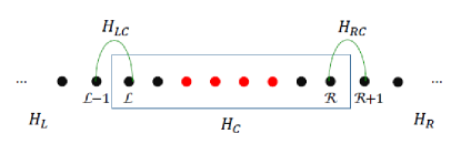
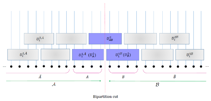
Although such studies on finite-size systems has created a deep insight into the MBL phase, practically we encounter with the systems of infinite length at the thermodynamic limit. So conducting a research which targets construction of LIOMs on an arbitrary long chain will made a great progress in this realm. To this end, as it is previously considered in some various studies Pekker01 ; Chandran02 ; Pollmann01 ; Wahl01 , one can utilize the localization of LIOMs in order to investigate a spin chain of infinite length in the MBL phase. It means that, instead of finding a unique unitary transformation for the entire system by diagonalization of the Hamiltonian in the total Hilbert space, LIOMs of the problem can be computed by means of tensor networks Pekker01 ; Chandran02 ; Pollmann01 ; Wahl01 . One of the suggested strategies, which has been presented in Ref. Kulshreshtha02 , introduces an algorithm, labeled the inchworm algorithm to calculate the expectation value of a product of local operators on a large system while working in a Hilbert space of computationally manageable size. We initialize the process using a subsystem on the rightmost window of length , then expand the system leftward and to keep the working space manageable, they subsequently contract the system from the right. Inspired by this method, we divide the Hamiltonian into five zones shown in Fig. 1, So, the Hamiltonian can be written as
| (5) |
where is the Hamiltonian of a region called central domain of length in which is decided to be calculated. In other words, if is the pseudo-spin defined on a site of the interval , in which is the middle of the central domain, is the Hamiltonian belonging to . is the Hamiltonian of the rest of the system in left side and is that of the right side. and are the interacting Hamiltonians between the left and right sides with the central part, respectively. These interaction Hamiltonians can be written in their explicit forms as
| (6) |
and
| (7) |
in which act on site as shown in Fig. 1. The essential point is that the Hamiltonians of and have no contribution in construction the desired pseudo-spin. Hence, for calculating , merely the consideration of will be sufficient and we are able to find exact LIOMs by using the scheme proposed in Ref. Adami01 for which reads
| (8) |
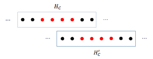
It should be noted that although diagonalization of the total Hamiltonian and obtaining belonging to this leads to the exact LIOMs, its generalization to the whole of the system violates the independence of pseudo-spins . This happens due to the fact that if we are going to compute th LIOM according to this method, we should utilize instead of and as the Fig. 2 shows obviously, these two Hamiltonians do not commute.
| (9) |
Therefore, the condition of orthogonality and independence of pseudo-spins and will not be held as well since they clearly do not satisfy the commutation relation. However, if the central-domain length is considered such that it is much greater than the localization length of LIOMs, the commutator magnitude will be very small and as a result, it can be completely neglected.
The other studious works which have been done to calculate such approximate LIOMs are Refs. Pollmann01 ; Wahl01 in which the authors have exploited the locality of integrals of motion and introduced tensor networks techniques by which such numerous local unitary transformations can be obtained. In Ref. Pollmann01 , a two-leg four-layer tensor network, using the variance of the energy summed over all approximate many-body eigenstates as their figure of merit, have been considered and in Ref. Wahl01 , the authors have made an effort to keep the layers in two by increase the number of legs and they have optimized the unitaries by minimizing the magnitude of the commutator of the approximate integrals of motion and the Hamiltonian, which can be done in a local manner. Although these mentioned studies have presented some very insightful analyses, the milestone is that minimization of their figure of merits directly to find the optimum unitaries impose a great deal of computational cost due to ascending number of parameters. Thus, implementing the procedure will be impossible for the systems of arbitrary length by increase the number of legs.
Equipped with what expressed above, let us now explain our noble and efficient scheme. Actually, we tend to acquire such that this LIOM satisfies the following relation,
| (10) |
In other words, we are looking for the LIOMs arisen from a unitary transformation which acts only in the central domain. The crucial point is that these obtained LIOMs need to be independent which means,
| (11) |
To this end, inspired by the tensor networks method proposed in Ref. Wahl01 used for the blocks of an arbitrary number of legs, we keep the number of layers in two and choose the length of the subsystem, on which is erected, ’even’ that we denote it by .
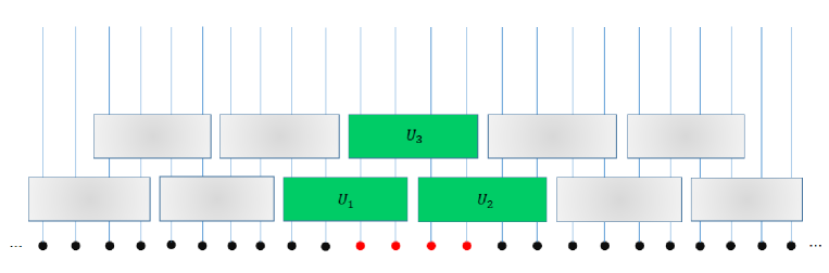
For the first layer, we divide this subsystem into two -leg blocks as half cut of the subsystem shown in Fig. 3. These blocks have the Hamiltonians of form of
| (12) |
and
| (13) |
where is the Hamiltonian of the left block and is that of the right one. By employing exact diagonalization, we will achieve two local unitary transformations. It is noticeable that to this end, we use the same method presented in Ref. Adami01 for finding the best permutation of the eigenstates to access the appropriate unitaries. Using such an approach to deal with the problem will intensively reduce the computational cost rather than the method utilized in Refs. Pollmann01 and Wahl01 and enable us to generalize our computations for the blocks on which exact diagonalization is numerically available. Thus, we have:
| (14) |
That being said, in order to obtain the Hamiltonian of the second layer let us complete our calculations as follows:
| (15) |
where is the Hamiltonian of the second layer defined on a -leg block in the middle of our determined subsystem. In this relation, to attain and , we need to project on the basis corresponding to the sites of and similarly will be projected on the basis related to the sites of for which we use the partial trace calculation techniques. Subsequently, expanding the Hilbert space upon the block of will be done for both and . Eventually, by writing in our new basis we will have an access to our desired correct . This goal is feasible as follows:
| (16) |
in which:
| (17) |
As pointed out before, the operator of also has to be projected on the basis of . Analogously, we will do the same procedure for and project it on the basis of . Ultimately, by expansion of the Hilbert space of those over the basis corresponding to the block of , these operators will be applicable to create the Hamiltonian of . Then by diagonalization of , one can achieve the unitary matrix related to the second layer and subsequently, by product of individual obtained unitaries we will be able to calculate a unique unitary for the entire approximately.
2.2 Efficacy of the method: how precise the approximate LIOMs are?
Having said that, it is inferred that can be attained using a local unitary transformation. This unitary transformation can be written in an explicit form of
| (18) |
where the unitary operator of only acts on the basis of central domain. Note that, if (where is the localization length of ), will be exact. However, in general case, if is of the same order of , is not accurate and therefore, we ought to introduce a criterion for investigating the precision of the pseudo-spin . In this work, we use the figure of merit defined in Ref. Wahl01 which reads
| (19) |
Before continuing the discussion, let us obtain the figure of merit, given in Eq. (19), for the physical spins themselves. Using Eq. (1), it is a simple practice to show that
| (20) |
and
| (21) |
where is the term of the Hamiltonian which does not commute with . It is easily indicated that
| (22) |
and . Hence,
| (23) |
and in the boundaries, this value is equal to . Now, we address the main question of this section. Indeed, we would like to calculate generally. To this end, using Eqs. (5)- (7), we have
| (24) |
where is the contribution of and is the participation of and altogether. It can be easily shown that
| (25) |
and
| (26) | ||||
A point of note is that the Hamiltonians of and have no participation in . Thus, to obtain , including leads to the appropriate result. Now, in order to gain a limit for , we suppose to look for a for the central domain such that it minimizes over the region of . In other words, we use a one-layer instead of two-layer unitary matrices. So, according to Eq. (8), we have and owing to the localization of the amount of has definitely a small value. We emphasize that diagonalization of the total Hamiltonian and finding exact pseudo-spins corresponding to this leads to the LIOMs for which is significantly small and it can be be taken into account as a limit for . In other words, by means of the scheme indicated in Fig. 3 we are not able to make the amount of less than that one of .
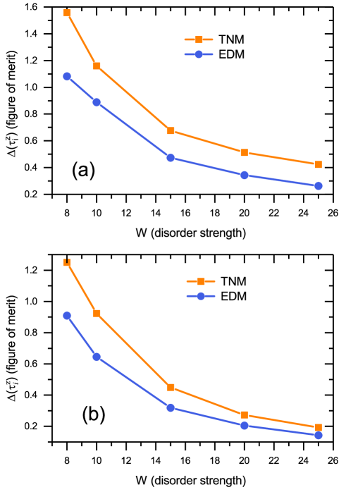
To answer the question that “how accurate are the results obtained from the proposed tensor-network approximation?”, one can calculate the values of the figure of merit, , by using this method and compare the obtained results with those corresponding values obtained from the exact diagonalization of the entire Hamiltonian. In figure 4, we have made a comparison between the numerical results obtained from the proposed tensor network representation with block lengths of 4 and 6 and those related to the exact diagonalization of a part of the Hamiltonian. From the physics of the problem, we expect that the results calculated employing the tensor network representation with a block length of are proportional to those obtained using the exact diagonalization for a chain of sites, and those for a block length of are proportional to the exact diagonalization for a chain of sites. As can be seen from the figure, the comparison shows that the results are completely consistent with our physical expectation. In other words, for obtaining the appropriate results of the Hamiltonian diagonalization by using the tensor network method presented here, one should consider the length of the blocks equal to the localization length of LIOMs of the specified system. This comparison emphasizes that by moving away from the phase transition point, it is possible to achieve the desired results by considering a normal length for the blocks in the tensor network. Another noteworthy point in figure 4 is that figure of merit, , decreases exponentially with increasing the disorder strength, W.
3 Calculation of the entanglement generation rate
One of the most outstanding features of the MBL systems is the existence of particular behaviour in the entanglement entropy generation rate in a bipartite system. Recently some precious studies have shed light on this characteristic of the MBL regime Znidaric01 ; Bardarson01 ; Serbyn02 ; Iemini01 ; Dumitrescu01 . Ref. Znidaric02 has studied entanglement dynamics in a diagonal dephasing model in which the intensity of interaction decays exponentially with distance and has calculated the exact expression for entanglement growth with time, obtaining in addition to a logarithmic growth, a sublogarithmic correction. Using the l-bit picture, correctly describes the MBL phase, implies that the entanglement in such systems does not grow (just) as a logarithm of time, as believed so far. Moreover, Chiaro and his co-workers Ref. Chiaro01 , using phase sensitive measurements, have experimentally characterized logarithmic entanglement growth of the MBL phase in such systems to determine the spatial and temporal growth of entanglement between the localized sites. In addition, they have studied the preservation of entanglement in the MBL phase. In this work, we are also going to demonstrate that our above-mentioned approach, presented in Sec. 2 to compute LIOMs, can be employed to calculate the entanglement generation rate and enables us to implement less numerical computations in a possibly short time. Generally, to investigate the generation of entanglement, inspired by some ever-done studies, we consider the initial state as
| (27) |
in which, given a chain of length , one can suppose that the subspaces and are the left half and the right half of the chain, respectively. We would like to have the largest entanglement generation rate. To this end, we focus on the initial state with zero expectation value of magnetization in the direction Znidaric02 ; Nanduri01 , i.e. and are . So, the time-dependent von Neumann entropy can be obtained via
| (28) |
where time-dependent reduced density matrix reads
| (29) |
Note that the above calculation can be done directly by means of exact diagonalization of the Hamiltonian and regardless of the LIOM concept. However, respecting to the exponentially growth of Hilbert space with the increasing number of sites and the necessity of performing numerical computations for various times, one can not choose the length of the chain more than sites due to the lack of computational resources.
In this section, we will indicate that, using the form of the transformations, we made in the previous section and by exploiting the concept of LIOMs: (a) the calculations in the MBL phase are independent of the length of the chain, and (b) with a much smaller amount of computations resulting in a manageable required memory and simultaneously with a fairly precise approximation, we are able to calculate the entanglement generation rate. According to Fig. 3, we assume that the Hamiltonian given in Eq. (1) with the blocks of sites has led to satisfactory results for Eq. (19), so that we can ignore the off-diagonal terms of the Hamiltonian. In other words, we approximate the Hamiltonian, on which the unitary transformations have been acted as follows:
| (30) |
Therefore, we can use the following relation to calculate in the physical-spin basis
| (31) |
To put it another way,
| (32) |
where and have been written in the LIOM basis. Note that to obtain the von Neumann entropy in the LIOM basis, entering (and ) in Eq. (32) is not required.
Before continuing the calculations, it deserves mentioning that, generally, is invariant under local transformations and , i.e. if
| (33) |
Another remarkable point is that if we consider diagonal approximation of the Hamiltonian in the LIOM space, as shown in Fig. 5, we have
| (34) |
in which and .
Hence, all the Hamiltonian terms commute together as they have been written in the LIOM basis. It is noticeable that and are the localized unitaries defined in the subspaces and , respectively. In other words, are the unitary operators of th block (by counting from bipartition cut, as the origin, to the left) corresponding to the subspace on the first layer and similarly, are the unitaries of th block (by counting from bipartition cut to the right) belong to the subspace on the first layer. In addition, are the unitary operators of block in the subspace and on the second layer (in which is excluded from labelling ) and are the ones of th block in subspace on the second layer. Thus, the only unitary operator between the subspaces and is illustrated in Fig. 5. Now, regarding to Fig. 2, it is obvious that is a local operator. So, by substitution of for in Eq. (33), Eq. (32) leads to
| (35) |
which results in the notion that the difference between the von Neumann entropy corresponding to the physical-spin basis and that of the LIOM basis is distinguished by . As the next step, we consider the local operator which commutes with . Thus, using the same procedure done for getting Eq. (35), one may reaches to
| (36) |
Ultimately, respecting to the commutation relation of (gray blocks in Fig. 5) with , the reduced density matrix of Eq. (36) can be written as:
| (37) |
where and , in which we show and as and , respectively. Consequently, to calculate the entanglement entropy, we just need to consider the blue blocks exhibited in Fig. 5 instead of the chain entirely.
That being said, the above calculations results in the following important achievement which is our main notion of this study: if the Hamiltonian is diagonalized with an arbitrary approximation under a tensor-network unitary transformation, to calculate the entanglement, it is sufficient to consider two blocks next to each other.
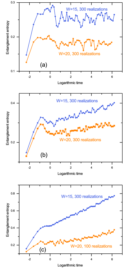
To show one of the efficient applications of the present tensor network method, we have investigated the time evolution of the entanglement entropy in the system for different block lengths using Eq. 37. For different values of the block length, and , the entanglement entropy, or von Neumann entropy has been plotted ve the logaritm of time. The results of the computations are displayed in figuur 6. As is seen from the figure, for a block length of 4, the behavior of the system is very simple. In the beginning, the system exhibits a rapidly changing behavior with time. The entropy of the system quickly reaches its maximum value and then it saturates to a given value. It has been shown that in an MBL system, the entanglement spreading has a logarithmic behavior with time, but in this case the amount of entanglement tends to a constant value so quickly. In fact, since the length of the block is smaller than the localization length of the LIOMs, the behavior we expect from an MBL system does not occur for this case. On the other hand, for a block length of 4, the available phase space for the entanglement spreading is very small, so we should not expect logarithmic behavior for this phenomenon.
For a block length of 8, both the localization length of the LIOMs is of the same order as the block length, and the available phase space for the entanglement spreading is more considerable. Consequently, the occurrence of logarithmic behavior for the entanglement spreading is not unexpected. For this case, such a logarithmic behavior can be seen for example for W=15 and/or for W=20 with different slopes. However, for W=20, the logarithmic spreading has a very small slope. For a block length of 12, the logarithmic behavior of the entanglement spreading can be observed. This observation is consistent with the results reported in Ref. Bardarson01 by Bardarson et al.
For an acceptable range of the disorder sterngth, , the comparison made in figure 6 shows that for the sufficiently large values of the block length, the local unitary matrices obtained from the approximate tensor-network method are compatible with those obtained from the exact diagonalization of the entire Hamiltonian.
In the end, it is necessary to note that although the present method has been carried out for the renowned XXZ model, it can be generalized to the other models for which the LIOMs can be defined. For example, this scheme can be implemented for a model of bond disordered XX-spin chain with long-range couplings and a lattice Schwinger model as well on which we are conducting our research as a future prospect.
4 Conclusion
A novel method for constructing the local unitary operators in the tensor network framework has been proposed, which allows us to obtain the unitary operator with high accuracy for blocks of very large length. The effective accuracy of the presented method has been examined and it has been shown that if the block length is larger than the localization length of the LIOM, then the entire Hamiltonian can be diagonalized with a high accuracy by the unitary operator of the tensor network. Finally, as an application of the proposed tensor network method, the spreading of the entanglement entropy of the system with time has been investigated. It is worth noting that for small block lengths, the entanglement spreading behavior is not obtained correctly and the entanglement entropy tends quickly to a constant value. But with the increase of the block length, the entanglement spreading exhibits such a behavior that is a characteristic of the MBL systems. When the block length increases to , for for the disorder strengthes of and , the behavior of the system is in very good consistent with the results of Bardarson et al, obtained using the exact diagonalization of the Hamiltonian and reported in Ref. Bardarson01 . Our study, firstly shows that the tensor network method with length can be used effectively for a large range of the disorder strength W, and secondly, the entanglement propagation reaches the limits of the block length of for large times. In other words, the logarithmic spreading of the entanglement is confined in a region of length for large times.
Data availability statement
The datasets generated and analyzed during the current study are available from the corresponding author on reasonable request.
References
- (1) Anderson, P.: Absence of diffusion in certain random lattices. Phys. Rev. 109, 1492 (1958)
- (2) Basko,D., Aleiner, I., Altshuler, B.: transition in a weakly interacting many-electron system with localized single-particle states. Ann. Phys. (Amsterdam) 321, 1126 (2006)
- (3) Oganesyan, V., Huse, D.: Localization of interacting fermions at high temperature. Phys. Rev. B 75, 155111 (2007)
- (4) Imbrie, J.Z., Ros, V., Scardicchio, A.: Local integrals of motion in many-body localized systems. Ann. Phys. (Berlin) 529, 1600278 (2017).
- (5) Pal, A., Huse, D.A.: Many-body localization phase transition. Phys. Rev. B 82, 174411 (2010)
- (6) Luitz, D.J., Laflorencie, N., Alet,F.: Many-body localization edge in the random-field Heisenberg chain. Phys. Rev. B 91, 081103 (2015)
- (7) Goihl, M., Gluza, M., Krumnow, C., Eisert, J.: Construction of exact constants of motion and effective models for many-body localized systems. Phys. Rev. B 97, 134202 (2018)
- (8) Serbyn, M., Papić, Z., Abanin, D.A.: Local conservation laws and the structure of the many-body localized states. Phys. Rev. Lett. 111, 127201 (2013)
- (9) Peng, P., Li, Z., Yan, H., Wei, K.X., Cappellaro, P.: Comparing many-body localization lengths via nonperturbative construction of local integrals of motion. Phys. Rev. B 100, 214203 (2019)
- (10) Adami, S., Amini, M., Soltani, M.: Structural properties of local integrals of motion across the many-body localization transition via a fast and efficient method for their construction. Phys. Rev. B 106, 054202 (2022)
- (11) Gholami, Z., Amini, M., Soltani, M., Ghanbari-Adivi, E.: Multibody expansion of the local integrals of motion: how many pairs of particle-hole do we really need to describe the quasiparticles in the many-body localized phase?. J. Phys. A: Math. Theor. 56, 155001 (2023)
- (12) Huse, D.A., Nandkishore, R., Oganesyan, V.: Phenomenology of fully many-body-localized systems. Phys. Rev. B 90, 174202 (2014)
- (13) Ros, V., Müller, M., Scardicchio, A.: Integrals of motion in the many-body localized phase. Nucl. Phys. B 891, 420 (2015)
- (14) Imbrie, J.Z.: On many-body localization for quantum spin chains. J. Stat. Phys. 163, 998 (2016)
- (15) Chandran, A., Kim, I.H. Vidal, G., Abanin, D.A.: Constructing local integrals of motion in the many-body localized phase. Phys. Rev. B 91, 085425 (2015)
- (16) Geraedts, S.D., Bhatt, R.N., Nandkishore, R.: Emergent local integrals of motion without a complete set of localized eigenstates. Phys. Rev. B 95, 064204 (2017)
- (17) Rademaker, L., Ortuno, M.: Explicit local integrals of motion for the many-body localized state. Phys. Rev. Lett. 116, 010404 (2016)
- (18) O’Brien, T.E., Abanin, D.A., Vidal, G., Papić, Z.: Explicit construction of local conserved operators in disordered many-body systems. Phys. Rev. B 94, 144208 (2016)
- (19) Kulshreshtha, A.K., Pal, A., Wahl, T.B., Simon, S.H.: Behavior of l-bits near the many-body localization transition. Phys. Rev. B 98, 184201 (2018)
- (20) Pekker, D., Clark, B.K.: Encoding the structure of many-body localization with matrix product operators. Phys. Rev. B 95, 035116 (2017)
- (21) Chandran, A., Carrasquilla, J., Kim, I.H., Abanin, D.A., Vidal, G.: Spectral tensor networks for many-body localization, Phys. Rev. B 92, 024201 (2015)
- (22) Pollmann, F., Khemani, V., Cirac, J.I., Sondhi, S.L.: Efficient variational diagonalization of fully many-body localized Hamiltonians. Phys. Rev. B 94, 041116 (2016)
- (23) Wahl, T.B., Pal, A., Simon, S.H.: Efficient representation of fully many-body localized systems using tensor networks, Phys. Rev. X 7, 021018 (2017)
- (24) Kulshreshtha, A.K., Pal, A., Wahl, T.B., Simon, S.H.: Approximating observables on eigenstates of large many-body localized systems. Phys. Rev. B 99, 104201 (2019)
- (25) Z̆nidarić, M., Prosen, T., Prelovs̆ek, P.: Many-body localization in the heisenberg xxz magnet in a random field. Phys. Rev. B 77, 064426 (2008)
- (26) Bardarson, J.H., Pollmann, F., Moore, J.E.: Unbounded growth of entanglement in models of many-body localization. Phys. Rev. Letters 109, 017202 (2012)
- (27) Serbyn, M., Papić, Z., Abanin, D.A.: Universal slow growth of entanglement in interacting strongly disordered systems. Phys. Rev. Lett. 110, 260601 (2013)
- (28) Iemini, F., Russomanno, A., Rossini, D., Scardicchio, A., Fazio, R.: Signatures of many-body localization in the dynamics of two-site entanglement. Phys. Rev. B 94, 214206 (2016)
- (29) Dumitrescu, P.T., Vasseur, R., Potter, A.C.: Logarithmically slow relaxation in quasiperiodically driven random spin chains. Phys. Rev. Lett. 120, 070602 (2018)
- (30) Z̆nidarić, M.: Entanglement in a dephasing model and many-body localization. Phys. Rev. B 97, 214202 (2018)
- (31) Chiaro, B., Neill, C., Bohrdt, A., Filippone, M., Arute, F., Arya, K., Babbush, R., Bacon, D., Bardin, J., Barends, R., Boixo, S., Buell, D., Burkett, B., Chen, Y., Chen, Z., Collins, R., Dunsworth, A., Farhi, E., Fowler, A., Foxen, B., Gidney, C., Giustina, M., Harrigan, M., Huang, T., Isakov, S., Jeffrey, E., Jiang, Z., Kafri, D., Kechedzhi, K., Kelly, J., Klimov, P., Korotkov, A., Kostritsa, F., Landhuis, D., Lucero, E., McClean, J., Mi, X., Megrant, A., Mohseni, M., Mutus, J., McEwen, M., Naaman, O., Neeley, M., Niu, M., Petukhov, A., Quintana, C., Rubin, N., Sank, D., Satzinger, K., White, T., Yao, Z., Yeh, P., Zalcman, A., Smelyanskiy, V., Neven, H., Gopalakrishnan, S., Abanin, D., Knap, M., Martinis, J., Roushan, P.: Direct measurement of nonlocal interactions in the many-body localized phase. Phys. Rev. Res. 4, 013148 (2022)
- (32) Nanduri, A., Kim, H., Huse, D.A.: Entanglement spreading in a many-body localized system. Phys. Rev. B 90, 064201 (2014)