Efficiency of Multivariate Tests in Trials in Progressive Supranuclear Palsy

Abstract

Objective: Measuring disease progression in clinical trials for testing novel treatments for multifaceted diseases as Progressive Supranuclear Palsy (PSP), remains challenging. In this study we assess a range of statistical approaches to compare outcomes measured by the items of the Progressive Supranuclear Palsy Rating Scale (PSPRS).

Methods: We consider several statistical approaches, including sum scores, as an FDA-recommended version of the Progressive Supranuclear Palsy Rating Scale (PSPRS), multivariate tests, and analysis approaches based on multiple comparisons of the individual items. In addition, we propose two novel approaches which measure disease status based on Item Response Theory models. We assess the performance of these tests under various scenarios in an extensive simulation study and illustrate their use with a re-analysis of the ABBV-8E12 clinical trial. Furthermore, we discuss the impact of the FDA-recommended scoring of item scores on the power of the statistical tests.

Findings: We find that classical approaches as the PSPRS sum score demonstrate moderate to high power when treatment effects are consistent across the individual items. The tests based on Item Response Theory (IRT) models yield the highest power when the simulated data are generated from an IRT model. The multiple testing based approaches have a higher power in settings where the treatment effect is limited to certain domains or items. The FDA-recommended item rescoring tends to decrease the simulated power in most test settings.

Conclusions: The study demonstrates that there is no one-size-fits-all testing procedure for evaluating treatment effects using PSPRS items; the optimal method varies based on the specific effect size patterns. The efficiency of the PSPRS sum score, while generally robust and straightforward to apply, varies depending on the specific patterns of effect sizes encountered and more powerful alternatives are available in specific settings. These findings can have important implications for the design of future clinical trials in PSP and similar multifaceted diseases.

Keywords Progressive Supranuclear Palsy, Clinical Trials, Multiple Endpoints, Simulation Study, Item Response Theory, Multivariate Tests

1 Introduction

In diseases that exhibit multifaceted manifestations, disease progression cannot be characterised with a single measurement. Instead, multiple characteristics have to be assessed to describe the disease status [1]. This poses a challenge to define appropriate endpoints in clinical trials to assess the effect of investigational treatments on the disease progression.

In this paper, we assess a wide range of statistical approaches that have been proposed to define and analyse endpoints for clinical trials in indications where disease progression is measured by several variables. We focus on the setting of clinical trials for Progressive Supranuclear Palsy (PSP), a rare neurodegenerative disorder with complex symptoms that affect balance, vision, body movements, and speech, ultimately leading to death. The most commonly used endpoint is the Progressive Supranuclear Palsy Rating Scale (PSPRS), a 28-item method to measure progression of the disease [2]. The item scores are categorical values which mostly vary from zero to 4. Recently, the FDA suggested to use only a subset of 10 item and to rescore some of the items into coarser categories (see Section 3.1 below). The PSPRS is then defined as a sum score, summing the item scores either of all 28-items (for the original score) or the subset of the 10 items suggested by FDA.

The use of a sum score, such as the PSPRS or its modifications, is a standard approach to combining information from multiple endpoints. By using such an aggregated score, standard statistical tests like an analysis of covariance can be applied to compare the outcome variable, or its change from baseline, between groups.

Another approach to demonstrate efficacy with an overall test involves multivariate testing procedures[3, 4]. These procedures aggregate test statistics of the comparisons of the individual characteristics into a single univariate test statistic and test the global null hypothesis that the treatments do not differ in any of the individual endpoints. [3] proposed two global directional tests known as Ordinary Least Squares (OLS) and Generalised Least Squares (GLS) tests to demonstrate an overall treatment effect [3]. Global directional tests are proposed in settings, where treatment benefit corresponds to a change into the same direction in all item scores. In such settings, two-sided tests as the Hotelling’s $T^{2}$ test, which does not account for the direction of treatment differences, is not of interest and will therefore not be considered further [5].

An alternative approach is to consider the individual components of the multivariate endpoint separately. In this case, inference is based on the individual test statistics or the individual p-values for the multiple endpoints and a multiplicity correction is applied to control the familywise error rate in the strong sense. This can be achieved by the Bonferroni procedure or more powerful multiple tests that take the dependence between the endpoints into account.

A further univariate test we consider is based on an Item Response Theory (IRT) model [6]. As endpoint we consider for each patient the value of the latent variable of the IRT model, which describes the disease status and can be predicted based on estimating the IRT model parameters given the data (or the scores). As the estimation of the latent variable from the item scores is complex we propose also to approximate the latent variable estimate using linear models. Specifically, we approximate the latent variable by a weighted sum of the item scores. This linear model-based estimation makes the endpoint better interpretable and yields a similar endpoint as the PSPRS sum score, however, using a weighted sum with weights derived from the IRT model (see Section 3.2).

We aim to identify the most powerful statistical tests to assess treatment effects under various scenarios. To compare the power of the different procedures, we perform a comprehensive simulation study. Especially, we consider different strategies to simulate data of the PSPRS item scores, including the discretisation of multivariate normal outcomes as well as resampling from actual clinical trial data from the ABBV-8E12 trial [7]. In addition, we consider a range of alternative hypotheses to cover settings where there is a treatment effect in all item scores or only in a subdomain or even in a single item score only. Additionally, we investigate the impact of the scoring of the items, suggested by the FDA, on the power of the considered statistical methods, as well as the case where the original scores are considered (See Section 3.1).

This paper is structured as follows: Section 3.1 describes the Progressive Supranuclear Palsy Rating Scale and its FDA modification. Section 2 discusses the ABBV-8E12 trial, forming the basis of our analysis. The considered analysis methods are detailed in Section 3.2, while Section 4 describes the different simulation approaches for the item level data as well as the simulation results. A re-analysis of the ABBV-8E12 trial is provided in Section 5. The paper concludes with a discussion in Section 6. Technical details on multivariate tests are provided in Section 1 of Supplementary Material.

2 Case Study

As case study to inform the trial designs and simulation of trial data in the simulation study, we considered the ABBV-8E12 trial [7]. The ABBV-8E12 trial was a randomised three-armed parallel group trial comparing a 2000mg and 4000mg dose of the investigational compound Tilavonemab to placebo.

In the ABBV-8E12 trial a total of 377 patients received at least one dose of the investigational treatment or placebo (Tilavonemab 2000 mg $n=126$, Tilavonemab 4000 mg $n=125$, placebo $n=126$). The original PSPRS items were assessed at baseline and weeks 12, 24, 36 and 52 where the change from baseline to week 52 in the PSPRS total score was the main outcome variable. In order to assess efficacy of treatments, the change from baseline to week 52 was analysed using a mixed-effect repeated measure model. The Bonferroni approach was used to account for multiplicity due to multiple comparisons between the two doses and placebo groups. The change from baseline to week 52 in PSPRS total score was similar between the three treatment groups at all considered visits and no significance difference between treatment groups, in favor of Tilavonemab 2000 mg or Tilavonemab 4000 mg versus placebo, at the two-sided significance level of 5% was observed.

To investigate the different testing approaches, below we considered a simplified study design with only one treatment-control comparison.

3 Methods

3.1 The Progressive Supranuclear Palsy Rating Scale (PSPRS)

Multiple clinical trials have been conducted to investigate the efficacy of therapeutic interventions in Progressive Supranuclear Palsy [7, 8, 9, 10, 11]. However, so far no symptomatic treatments or disease-modifying therapies are available [12, 13].

In randomised, phase 2, placebo-controlled trials of experimental treatments of PSP, the standard method to test for a treatment effect is to use the sum of the 28 item scores (the so called total score) of the Progressive Supranuclear Palsy Rating Scale (PSPRS) as the primary endpoint variable. Changes in this endpoint are compared between treatment groups, with higher scores indicating more severe disease conditions. Recently, the FDA has recommended to use a modified version of the PSPRS, which includes a subset of 10 items (Table 1). Each item in this subset is assigned a score ranging from zero to 4. Note that the score is based on the physicians’ assessment and is measured repeatedly to assess disease progression across different visits in the trials.

In addition, FDA recommended to collapse some of the item levels of the 10-item version of the PSPRS. A re-scoring has been recommended by FDA for all but two items, since it was argued that the original response levels for some items do not reflect clear and clinically meaningful differences of the patients’ conditions and are therefore difficult to interpret. Throughout the remainder of the text, we refer to the original and rescored item levels as the "original scores" and the "FDA scores". The full version of the PSPRS (with 28 items) which includes the subset of 10 items suggested by the FDA is provided as a table in the online Supplement B. The table contains the original scores and the FDA scores, including a description on how to collapse the item levels.

Table 1: FDA-recommended 10-item version of the PSPRS. The 10 items are divided into 3 domains (History, Bulbar exam, Gait/Midline Exam). The numbering of the items corresponds to the original PSPRS score [2]. The column "Abbreviation" gives the short name used to label the items in the subsequent graphs.

Full name	Abbreviation
i@. HISTORY (from patient or other informant)
3. Dysphagia for solids (from patient or other informant)	Dysp.FS
4. Using knife and fork, buttoning clothes, washing hands and face (rate the worst)	Use.KF
5. Falls (average frequency if patient attempted to walk unaided)	Fall
iii@. BULBAR EXAM
12. Dysarthria (ignoring palilalia)	Dysa.
13. Dysphagia (for 30-50 cc of water from a cup, if safe)	Dysp.
vi@. GAIT/MIDLINE EXAM
24. Neck rigidity or dystonia	Neck.Ri
25. Arising from chair	Ari.FC
26. Gait	Gait
27. Postural stability (on backward pull)	Pos.St
28. Sitting down (may touch seat or back but not arms of chair)	Sit

In this work we focus on the item scores of the 10 items proposed by FDA. This is also supported by a statistical assessment of the 10 items based on IRT analysis, which also suggests that these items are the most informative to describe the course of the disease [14].

Additionally, as in the ABBV-8E12 trial [7], we assume that the primary endpoint is based on the item scores measured at week 52, accounting for the baseline, corresponding to a one year observation period.

3.2 Analysis methods

All the analyses below were performed based on the subset of 10 FDA recommended items of the PSPRS with the original scoring as well as the FDA re-scoring.

With the exception of the IRT based test (but not the approximate IRT based test), all tests below test the null hypothesis that the expected values of all of the FDA recommended item scores are larger or equal in the treatment group than in the control group. We term this null hypothesis as the strong null hypothesis. The corresponding alternative hypothesis is that the expected values of at least one item scores is strictly smaller in the treatment group compared to the control group. Some of the tests in addition are valid tests for broader null hypotheses as indicated below.

PSPRS Scores

As benchmark, we used an analysis of covariance (ANCOVA) for the PSPRS sum score at week 52 as dependent variable and the PSPRS sum score at baseline as well as the treatment indicator as independent variables. The (t-)test for the coefficient for the treatment variable then tests the null hypothesis of no treatment effect. Note that this adjusted analysis is equivalent to a between group comparison of the change from baseline between the two groups. This test not only tests the strong null hypothesis, but also the null hypothesis that the mean of the item scores (across items and the patient population) is larger or equal in the treatment compared to the control group.

IRT-based test

The second considered, univariate test is based on estimates of the latent variable based on an IRT model [15]. IRT models represent the state of disease as a latent variable which is defined based on multiple reported measures. In PSP, the latent variable corresponding to the disease severity is measured through the PSPRS item questionnaire as reported by the physician. To perform the IRT-based test, we require an IRT model fitted on an external data set. We used a graded response (GR) model, fitted to the ordered polytomous data [16] scores of the FDA-recommended 10-item version of the PSPRS from the ABBV-8E12 trial. To this end, we first pooled the data across treatment groups and visits (including the baseline and follow-up visits at weeks 12, 24, 36 and 52) such that the data from each visit became an independent individual (row) in the data set. Based on this data set, we fitted an IRT model. The parameter estimates of the GR model are presented in Table 1 of Supplementary Material A. This simplified analysis does not account for the dependence of the measurements from a patient at different visits, but accounts for the dependence of a patient’s measurements of the different items within a single visit. This allowed to estimate the IRT model based on a larger data set with the aim to enhance the precision of the model estimates.

Based on this a-priori estimated model, we then estimate the latent trait variable for the patients in the actual clinical trial based on the observed item scores, separately for the baseline and the 52-weeks data. Especially, we estimate the predicted latent trait variable with the expected a-posteriori (EAP) method [17], which is implemented, for example, in the R package mirt for the analysis of dichotomous/polytomous response data using latent trait models under the IRT paradigm [18].

Finally, an ANCOVA model is fitted with the predicted latent trait variable at week 52 as dependent and the latent trait variable at baseline and treatment as independent variables. This procedure tests the null hypothesis that the expected value of the latent variables is larger in the treatment group than the control group.

This procedure tests the null hypothesis that the expected values of the latent variable estimate in the treatment group is larger or equal than in the control group. Especially, this null hypothesis holds, if the joint distribution of item scores in the two treatment groups is equal. However, given the complex dependence of the latent variable estimates on the item scores, it is not obvious if this null hypothesis is included in the strong null hypothesis defined above.

Approximate IRT-based test

As the estimation of the latent variable with IRT model is complex and the impact of the individual item scores is not immediately understandable without going through complex derivations, we aim to approximate the estimate by a weighted sum of the item scores. This aims to make the endpoint better interpretable. Therefore, we consider as endpoint a weighted sum of the item scores, where the weights are derived from a linear model fitted on the data of an external trial. We used again data of the ABBV-8E12 trial, where, as above, we aggregated the data from all treatment groups and visits, fitted and IRT model and estimated the latent variable for each patient. Then, using the same data set, we fitted a linear model with the latent variable as dependent variable and the 10 FDA recommended items as independent variable. Note that the latent variable was transformed with the standard logistic function to improve model fit. Based on this a-priori estimated model, we then estimate the (approximate) latent trait variable for the patients in the actual clinical trial by computing the weighted sum of the observed item scores and back transforming it (using the standard logit function) to match the original scale. Note that in principle the linear model could give values outside the unit interval such that the standard logit function cannot be applied. If this occurs one can truncate the values accordingly. For our data set this was not an issue as the corresponding fitted linear model only gives values in the unit interval. In addition to the strong null hypothesis defined above, this procedure tests the null hypothesis that the expected value of the resulting weighted sum score is larger in the treatment compared to the control group.

OLS and GLS tests

The [3]’s OLS and GLS tests [3] are multivariate tests combining test statistics of separate tests comparing the responses for each of the items between groups to a common test statistics. The OLS test is based on the standardised, unweighted sum of t-statistics of the individual items, see Eq. (1) in Supplementary Material A. The GLS test, in contrast, is based on a weighted sum, determined by the row sums of the inverse of the correlation matrix (see Eq. (2) in Supplementary Material A). The t-statistics for the comparison of the individual item scores are obtained from an ANCOVA model, with the item score at week 52 as the dependent variable and the baseline item score and treatment indicator as independent variables. The correlation of the test statistics, required to standardize the test statistics and, for the GLS test, to compute the weights, is estimated using multiple marginal modeling (using the mmm function [19] in the multcomp package in R). Endpoints that are highly correlated receive lower weights in the GLS test statistic. For very high correlations, the weights may even become negative. This implies that the corresponding test may no longer be a directional test but can inflate the type I error rate if there is a negative effect in some of the items and no effect in the others. Thus, the GLS test controls the type 1 error rate under the strong null hypothesis only if all weights are non-negative. When re-analysing the ABBV-8E12 trial, we observed a negative weight for one item and therefore considered a modified GLS test, where we dropped this item (see Section 5). Following the recommendation of [20], for the OLS and GLs tests we used a modified approximation of the degrees of freedom (df) setting $df=0.5(2n-3)(1+1/m^{2})$, where $n$ is the per-group sample size and $m$ the number of items. This has been shown to provide better control of the type I error rate for smaller sample sizes (see Supplementary Material A, Subsection 1.1) compared to the original proposal by O’Brien.

Bonferroni test

An alternative approach to computing cumulative test statistics, based on individual tests for each item (as the OLS or GLS test), is to consider the results of each of the individual tests separately and to apply a multiplicity adjustment to control the FWER. Individual t-statistics (and the associated un-adjusted p-values) are obtained from multiple marginal models as described above. Then an adjusted significance level is applied. The overall null hypothesis of no treatment effect in any item, is rejected if the smallest p-value across all items falls below the Bonferroni adjusted significant level (which is $\alpha/10$, as 10 items are considered). An advantage of this approach is that it also provides a test to compare the item scores for each item: One can reject the null hypothesis of no treatment effect for an item, if the corresponding p-value falls below the Bonferroni adjusted significance level. A further improvement for the individual tests can be obtained by applying the Bonferroni-Holm test.

Hommel/Simes test

Similar to the Bonferroni test, also other multiple testing procedures can be applied to test the overall null hypothesis. An example is the Simes [21] test for the global null hypothesis of no treatment effect in any item (and its closure the Hommel test [22], to obtain tests for the individual items). This test is, for example in the R package hommel. For these tests control of the type I error rate has been shown for independent test statistics as well as test statistics with certain positive correlation structures.

Omnibus test

The Omnibus test [23] is an alternative test for the global null hypothesis of no treatment effect in any item which is based on individual test statistics. This test has shown to have robust power both in settings where for a few or for many null hypotheses the alternative hypothesis holds false. It is based on cumulative sums of (reciprocal) transformed sorted p-values. Note that theoretical type I error rate control for these tests has been shown for independent test statistics only.

Omnibus test for domain scores

The 10 items of the PSPRS scale are divided into three domains (see Table 1). For this test we first compute the sum-score across items for each domain. We then perform the ANCOVA analysis for each of the resulting three domain scores and then adjust for multiplicity using the Omnibus test as above.

MaxT test

The Bonferroni approach is strictly conservative as it does not take into account the correlation of test statistics. Based on the estimated correlation of t-statistics one can use a test based on the individual t-values which takes into account the correlations. To improve the accuracy of the subsequent normal approximation, we first replace the t-values by transformed z-values to take into account the degrees of freedom, setting $z_{i}=\Phi^{-1}(F_{t,df}(-t_{i})),i=1,\dots,10$, where $\Phi^{-1}$ and $F_{t,df}$ denote respectively the quantile function of the normal distribution and the CDF of the t-distribution.

Since low values of the item scores correspond to a better outcome, small (negative) t-values or equivalently large (positive) z-values, as defined above, indicate a beneficial treatment effect. Therefore, the test statistics to test the overall null hypothesis of no (beneficial) treatment effect in any item, is defined as the maximum of the z-statistics. Then, the multiplicity adjusted p-value is obtained, based on the distribution function of the multivariate normal distribution and is given by $P_{\boldsymbol{Z}_{\max}}=1-P_{\boldsymbol{\Sigma}}(\boldsymbol{Z}\leq\boldsymbol{z}_{\max})$, $\boldsymbol{Z}\sim\mathcal{N}(\boldsymbol{0},\,\hat{\boldsymbol{\Sigma}})\,$ where $\boldsymbol{z}_{\max}=\left(z_{\max},\dots,z_{\max}\right)$, $z_{\max}=\max(z_{1},\dots,z_{10})$ and the correlation matrix $\hat{\boldsymbol{R}}$ is estimated using multiple marginal models as above (see the paragraph on OLS and GLS tests).

The considered analysis methods are summarized in Table 2.

Table 2: The considered analysis methods: category of the method (first column), name of the analysis method (second column), short name used to label the method in the result section (third column), and description for each test (fourth column).

Category	Name	Abbreviation	Description
Univariate test statistic (of aggregated scores )	Sum Score	SumS	Sum of the item scores is used as the dependent variable.
	IRT-based test	IRT.PSIF	IRT-based estimate of the latent variable is used as the endpoint.
	Linear model-based test	LM.PSIBPF	uses a linear model-based estimate of the latent variable, with a weighted sum of the item scores, as the endpoint.
Weighted test statistic composed of that of the individual items.	O’Brien’s OLS test	OLS	sum of t-statistics of the individual items with equal weights (see Supplementary Material A, Subsection 1.1).
	O’Brien’s GLS test	GLS	sum of t-statistics of the individual items with unequal weights (see Supplementary Material A, Subsection 1.1).
	O’Brien’s GLS test	GLS-26	the GLS test based on 9 items (after eliminating item 26).
Individual (item) test statistic	Bonferroni correction	Bonf	based on the smallest p-value across the individual test statistics of the 10 items.
	maximum T-value	MaxT	based on the largest (transformed) t-value among the 10 items.
	Simes	Simes	based on individual adjusted p-values from the items.
	Omnibus	Omnibus	based on cumulative sums of the transformed sorted p-values when there is no a priori knowledge on the number of false individual null hypotheses.
	Combination test: Omnibus and Sum Score	Omnibus-dom	a combined test applying the sum score test within each of the domains and the Omnibus test between them.

4 Simulation Study

To evaluate the operating characteristics of the considered analysis methods, we conducted a large scale simulation study using three approaches to simulate individual item scores of the FDA-recommended subset of items of the PSPRS. This allows us to assess the robustness of findings with respect to specific assumptions of the data generating process. Especially, we generated data (1) from a discretised multivariate normal distribution, (2) with a Bootstrap approach based on the ABBV-8E12 study, and (3) based on a longitudinal IRT model. As no differences between groups were observed, we used pooled (across treatment groups) estimates of the outcomes distribution and also pooled the groups to generate the Bootstrap samples (see the description below).

4.1 Simulation of the item level data

Below, we describe the three data simulation approaches in detail. Table 3 summarizes the key aspects of the different approaches.

All the simulation methods yielded scores using the original scoring of the items. To generate items according to the FDA re-scoring, we collapsed in a further step the corresponding item levels. In the simulations we considered a trial with an experimental treatment and a control arm, assuming a per-group sample size of $n=70$. For each scenario $10.000$ trials were simulated.

Table 3: Parameter specifications for simulation studies.

Name	Type	Values	Description
Analysis type	Design choice	two covariates	Analysis is based on ANCOVA models including the treatment effect and the relevant baseline value, to the analysis methods summarized in Table 2, as covariates.
Total sample size per treatment	Design choice	70 per treatment group	The sample size is fixed across simulation approaches.
Number of simulations runs	Assumption	10000 per simulation approach	The number of simulations runs is fixed across simulation approaches.
Nominal significance level	Assumption	$\alpha=0.025$	The one-sided nominal significance level is fixed in all analysis methods and across simulation approaches.
Parametric simulation method: discretised item scores	Assumption	effect sizes are either fixed/varied across all items or fixed across domains (details in Table 4)	First, data is generated from the multivariate normal distribution (see details in Subsection 4.1). It is then discretised to the nearest integer (and bounded from 0-4) to perform the analysis tests.
Non-parametric simulation approach: Bootstrap (without replacement)	Assumption	effect sizes are either fixed/varied across all items or fixed across domains (details in Table 4)	Data sets are resampled based from the ABBV-8E12 study at baseline and Week 52 (Section 3)
IRT-based simulation method	Assumption	effect sizes are fixed in all items. Multiple ratios of the progression equation, $\rho$ values (details in Subsection 4.1), are investigated as $0.45$, $0.50$, $0.55$, $0.60$, $0.65$, $0.70$, $0.75$.	Subjects are sampled from the ABBV-8E12 data. Subsequently, corresponding relevant covariates are used to construct the progression equation and generate the IRT-based item level data (details in Subsection (Section 3).

Discretised multivariate normal distribution

To parameterize the simulation distribution, we estimated the $20\times 1$ mean vector and $20\times 20$ covariance matrix of the item scores at baseline and Week 52 from the ABBV-8E12 trial data. Especially, the control mean was estimated based on the data of the placebo group and the co-variances were estimated in each of the three treatment groups and then a pooled estimate, $\hat{\boldsymbol{\Sigma}}_{p}$, was computed, weighting according to the sample sizes.

Then, to generate the control group data, we drew vectors from a multivariate normal distribution with mean $\hat{\boldsymbol{\mu}}_{3}$ and covariance $\hat{\boldsymbol{\Sigma}}_{p})$. Similarly, the experimental treatment groups data was drawn from a multivariate normal distribution with the same covariance matrix but mean $\hat{\boldsymbol{\mu}}_{3}-\boldsymbol{d}$, where $\boldsymbol{d}$ denotes the vector of effect sizes across items.

The vectors sampled from the normal distributions are then discretised by rounding, and trimming the scores to the range 0 to 4.

Bootstrap

We resampled subjects from the ABBV-8E12 study and considered both, resampling with and without replacement, but report here only the results of the latter as both provided similar results. Resampling was performed from the complete cases (where all items at the baseline and Week 52 visit were available) pooled across all three treatment groups. Then subjects of the control group and the experimental treatment group were sampled from this data set. For simulations under the alternative hypothesis, for the subjects sampled in the experimental treatment arms the item scores at Week 52 were adjusted by the assumed treatment effect. Especially, for an effect size $d_{k}$ and item scores $y_{k,i}$ for item $k=1,...,10$ and subject $i=1,\ldots,n$ in the experimental treatment group, where $n$ is the per group sample size of the simulated sample, we adjust the scores $y_{k,i}$ such that the mean effect in the population (up the floor effects due to the bounded scale) is approximately $d_{k}$. This is achieved setting

1. For all $k=1,\ldots,10$ and $i=1,\ldots,n$, set $y_{k,i}\to y_{k,i}-\lfloor d_{k}\rfloor,$ where $\lfloor d_{k}\rfloor$ denotes the floor value of the individual item effect size $d_{k}$.

2. Randomly select a subset of $np_{k}$ (rounded to the nearest integer) subject indices, denoted by $I_{k}$, where $p_{k}=d_{k}-\lfloor d_{k}\rfloor$ and set $y_{k,j}\to y_{k,j}-1$ for all $j\in I$.

3. Finally, trim the scores to the range of the scale, setting $y_{k,i}\to max(0,y_{k,i})$ for all $k=1,\ldots,10$ and $i=1,\ldots,n$.

IRT model based data generation

We simulated item level data for the baseline and Week 52 item scores based on the longitudinal IRT model of [14] fitted on multiple data sets from a set of interventional trials in PSP. They used a 2-parameter graded response (GR) model (see, e.g., Equation 4 in [16]) based on discrimination and difficulty as item characteristic parameters. The GR model was fitted to the ordered polytomous data, scores of the FDA-selected subset of items (but ignoring the rescoring recommendation) from the PSPRS in all interventional studies. The underlying latent variable at time $t$, in years, is represented through a disease progression model for individual $i$, given by

$$\psi_{i}(t)=\psi_{i}(0)+s_{i}t$$

where $\psi_{i}(0)$ and $s_{i}$ respectively denote the intercept and slope. For a subject $i$, intercept and slope are given as a function of relevant baseline and slope covariates of the patient, as age, sex, and PSP diagnostic phenotype (see [14] for a detailed description of the derivation of the corresponding prediction model). To model disease progression under the alternative, for patients in the treatment group, we assumed a smaller slope in the longitudinal latent variable model. Especially, we assumed that the latent variable evolves as $\psi_{i}(0)+\rho s_{i}t$ , where $\rho<1$ indicates a beneficial treatment effect.

To simulate the data we sampled subjects from the ABBV-8E12 study and based on the covariate information of the sampled subjects, we computed for each subject the predicted latent variable at baseline and Week 52. Based on these latent variables we then simulate the individual item scores using the items discrimination and difficulty parameter as estimated in [14].

4.2 Considered treatment effect scenarios

The performance of the different testing approaches depends on the pattern of treatment effects across the items. We therefore considered a range of treatment effect patterns. For the simulations based on discretised multivariate normal samples and the Bootstrap approach, the considered effect size scenarios are given in Table 4 and include the case of small, intermediate, and strong equal absolute effects across items ($\boldsymbol{d}_{1}^{\prime},\boldsymbol{d}_{2}^{\prime},\boldsymbol{d}_{3}^{\prime}$). Here, $\boldsymbol{d}_{l}^{\prime},l=1,\dots,12$ denote the transposed treatment effect vectors across items. We further considered scenarios ($\boldsymbol{d}_{4}^{\prime}-\boldsymbol{d}_{9}^{\prime})$ where there the treatment effect is limited to items in a single or two domains. Within each domain, the absolute treatment effects are assumed to be equal. For instance, in $\boldsymbol{d}_{5}^{\prime}$ we assume an equal absolute treatment effect in each the FDA-recommended items in the History Domain (items 3, 4 and 5). As a reference, we have also included three scenarios in which the treatment effect is isolated to a single item ($\boldsymbol{d}_{10}^{\prime}-\boldsymbol{d}_{12}^{\prime})$.

For the data generated with the IRT model, we considered different effects on the slope of the latent variable, and specified $\rho$ as $\rho=\{0.45,0.5,0.55,0.6,0.65,0.7,0.75\}$ which leads to power values that allow to discriminate results in the statistical tests with respect to power.

Table 4: Effect size scenarios considered in the simulation study. The rows correspond to vectors $\boldsymbol{d}$ of effect sizes for the 10 items in the FDA recommended modification of the PSPRS scale.

		Dysp.FS	Use.KF	Fall	Dysa	Dysp.	Neck.Ri	Ari.FC	Gait	Pos.St	Sit
Equal effect size	$\boldsymbol{d}_{1}^{\prime}$	$0.20$	$0.20$	$0.20$	$0.20$	$0.20$	$0.20$	$0.20$	$0.20$	$0.20$	$0.20$
Equal effect size	$\boldsymbol{d}_{2}^{\prime}$	$0.25$	$0.25$	$0.25$	$0.25$	$0.25$	$0.25$	$0.25$	$0.25$	$0.25$	$0.25$
Equal effect size	$\boldsymbol{d}_{3}^{\prime}$	$0.30$	$0.30$	$0.30$	$0.30$	$0.30$	$0.30$	$0.30$	$0.30$	$0.30$	$0.30$
History domain	$\boldsymbol{d}_{4}^{\prime}$	$0.85$	$0.85$	$0.85$	$0.00$	$0.00$	$0.00$	$0.00$	$0.00$	$0.00$	$0.00$
Bulbar exam	$\boldsymbol{d}_{5}^{\prime}$	$0.00$	$0.00$	$0.00$	$1.25$	$1.25$	$0.00$	$0.00$	$0.00$	$0.00$	$0.00$
Gait/midline exam	$\boldsymbol{d}_{6}^{\prime}$	$0.00$	$0.00$	$0.00$	$0.00$	$0.00$	$0.50$	$0.50$	$0.50$	$0.50$	$0.50$
History domain & Bulbar exam	$\boldsymbol{d}_{7}^{\prime}$	$0.50$	$0.50$	$0.50$	$0.50$	$0.50$	$0.00$	$0.00$	$0.00$	$0.00$	$0.00$
History domain & Gait/midline exam	$\boldsymbol{d}_{8}^{\prime}$	$0.30$	$0.30$	$0.30$	$0.00$	$0.00$	$0.30$	$0.30$	$0.30$	$0.30$	$0.30$
Bulbar & Gait/midline exam	$\boldsymbol{d}_{9}^{\prime}$	$0.00$	$0.00$	$0.00$	$0.35$	$0.35$	$0.35$	$0.35$	$0.35$	$0.35$	$0.35$
Dysphagia for solids (in History domain)	$\boldsymbol{d}_{10}^{\prime}$	$2.50$	$0.00$	$0.00$	$0.00$	$0.00$	$0.00$	$0.00$	$0.00$	$0.00$	$0.00$
Dysarthria (in Bulbar exam)	$\boldsymbol{d}_{11}^{\prime}$	$0.00$	$0.00$	$0.00$	$2.50$	$0.00$	$0.00$	$0.00$	$0.00$	$0.00$	$0.00$
Neck rigidity (in Gait/midline exam)	$\boldsymbol{d}_{12}^{\prime}$	$0.00$	$0.00$	$0.00$	$0.00$	$0.00$	$2.50$	$0.00$	$0.00$	$0.00$	$0.00$

4.3 Results of the simulation study

In the simulation study, we assessed the type I error rate and power of each of the analysis methods for the different data generating procedures and treatment effect scenarios.

None of the considered methods showed an apparent inflation of the type I error rate in the considered scenarios (see Figure 1). This holds for all three simulation approaches and the original item scoring as well as the tests based on the rescored items.

Figure 2 summarizes the power of the different methods across all simulation approaches and effect size scenarios, both for the original scoring of the items as well as the FDA-rescoring. Based on 10000 simulations runs, the standard error of the power estimates is bounded from above by 0.005. To better distinguish the scenarios, separate plots for different treatment effect scenarios and data simulation approaches are given in the Figures 1 and 2 in the Supplementary Material A.

Comparison of testing procedures

In treatment effect scenarios where there is a homogeneous absolute effect in all items (Scenarios $\boldsymbol{d}_{1}^{\prime}$, $\boldsymbol{d}_{2}^{\prime}$ and $\boldsymbol{d}_{3}^{\prime}$) we observe the highest power for the test based on the classical PSPRS sum score using the original scores. This holds for data simulated with Bootstrap as well as data simulated from the multivariate normal distribution. Similarly, the GLS test and its modification excluding item 26 (Gait) show high power values. However, even after eliminating this item, we observed negative weights for other items in simulated data sets, which causes issues in interpretation. In scenarios with homogeneous effects, also the test using the latent variable estimate from the IRT model as well as its approximation (with slightly lower power) and the Omnibus test based on the domain sum score show a good performance. In contrast, the other tests based on multiple testing procedures had substantially lower power.

On the other hand, when there is an effect only in certain domains or individual items, the power of tests based on multiplicity adjusted separate tests have the highest power. Here, the power of the test based on the PSPRS sum score is lower. The tests based on the IRT model have low power if there is an effect in a single domain or single item only. In considered scenarios where the effect is in two domains, the power was higher than with the PSPRS sum score. The Omnibus-dom test has a large power in scenarios where the effect size is homogeneous within one or more domains, but lower power than the other multiple testing procedures if the effect is in a single item only.

When simulating the data using the longitudinal IRT model, for all considered effect sizes (determining the change of the slope of the latent variable), the analysis based on the IRT model performed best in terms of power, followed by the approximate IRT model based on the weighted sum of the item scores. In these settings, also the original PSPRS sum score, the OLS test and the Omnibus_dom test showed a good performance. Note that in the IRT model, the treatment effect is modelled directly for the latent variable which corresponds to a treatment effect in all items.

Original scoring vs. rescoring

For most of the tests we observe that the FDA scoring causes a drop in the simulated power, specifically in scenarios where there is a homogeneous effect in all items (Scenarios $\boldsymbol{d}_{1}^{\prime}$, $\boldsymbol{d}_{2}^{\prime}$ and $\boldsymbol{d}_{3}^{\prime}$). This might be due to a loss of information by collapsing item levels. For the analysis method based on the IRT models, however, there are also scenarios where the treatment effect is in single domains only, where the power appears to increase after re-scoring. In the simulations based on the IRT model there is a tendency for a decrease in power with the rescored data.

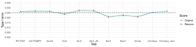
(a) Discretised multivariate normal distribution

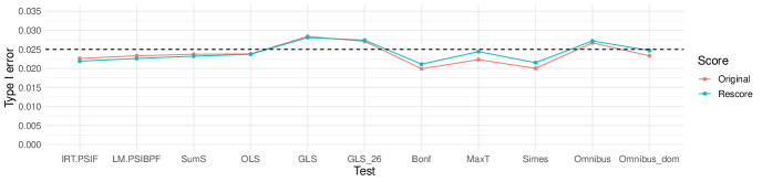
(b) Bootstrap (without replacement)

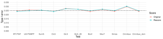
(c) Item scores generated from the IRT model

Figure 1: Type I error rates of the hypothesis tests for the different simulation approaches. The dashed lines represent the nominal significance level of 0.025 (one-sided). With 10 000 simulation runs, standard error of the estimated type I error rates (when the actual type I error is 0.025) is 0.00156. Thus, none of the methods shows an apparent inflation of the type I error rate.

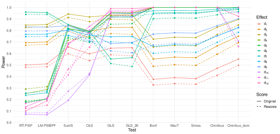
(a) Discretised item scores generated from multivariate normal distribution

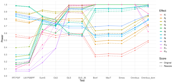
(b) Bootstrapped item scores (without replacement)

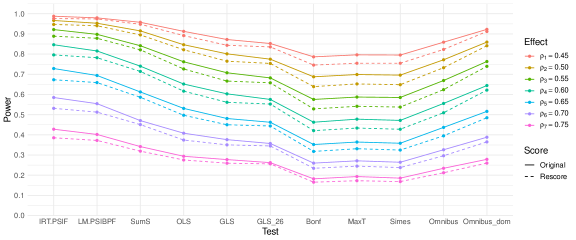
(c) Item scores generated from the IRT model fit

Figure 2: Power of the considered testing procedures for all simulation approaches and effect size scenarios.

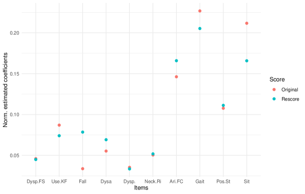
Figure 3: Linear model fit of the latent variable. The plot shows the normalised weights (summing to one) for the items with the original (red) and the FDA-recommended rescoring (blue).

(a)

(b)

Figure 4: Scatterplot of the transformed estimated latent traits from the IRT model fit and the fitted values from the linear model of items.

5 Reanalysis of the ABBV-8E12 trial

To illustrate the application of the different analysis methods, we re-analyse the ABBV-8E12 trial with the analysis methods considered above, we compare each dose (tilavonemab 2000, tilavonemab 4000) to placebo, in separate analyses. We included $66$, $71$, and $64$ patients in the tilavonemab 2000, tilavonemab 4000, placebo groups respectively, for which both the baseline and the Week 52 data were available for all the FDA subset of items. Note that in this data set there is a substantial proportion of missing values of item scores in later visits, specifically in Week 52, compared to baseline. This is due to the fact that the whole study was terminated early as no differences between the dose groups compared to placebo were observed in an interim analysis. Table 5 shows the descriptive statistics of the baseline and Week 52 item scores as well as the treatment effect estimates and corresponding p-values from marginal ANCOVA models with the Week 52 scores as dependent variable and the baseline score and treatment as independent variables.

Results of the different hypotheses tests defined in Section 3.2 are given in Table 7. While, in agreement to the original analysis, none of them indicates a significant difference between groups, we find that the testing procedures yield a wide range of p-values. This reflects the fact, that the different tests focus on different aspects of deviations from the null hypothesis.

To assess the latent variable estimates obtained by a weighted sum of the item scores used in the approximate IRT-based test (Section 3.2) we visually inspected the model fit, both, for the linear model fitted to the original and the rescored items. Especially, we plot the latent variable estimate based on the linear model fit against the estimates obtained with the EAP method in the ABBV-8E12 data set, pooling the data from all visits and treatment groups as described above (see Figure 4). The figure shows that, when computing the latent variables based on the original item scores, we observe a nearly perfect model fit with minimal errors. Estimating the latent variable based on a weighted sum of the rescored items yields a somewhat larger error, especially for small values of the latent trait. The weights of the items in the resulting linear models are depicted in Figure 3 with the largest weights allocated to the items ’arising from chair’, ’gait’, ’postural stability’ and ’sitting down’ from the gait/midline exam domain.

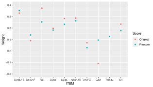
(a) Tilavonemab 2000 vs placebo

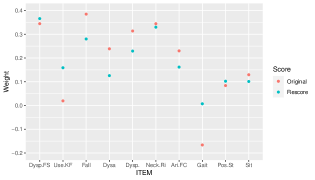
(b) Tilavonemab 4000 vs placebo

Figure 5: Weights of the individual test statistics in the GLS test in the re-analysis of the ABBV-8E12 trial.

The weights for the individual t-statistics in the GLS test are given in Figure 5a. For the original scores, the weight of item 26 (Gait) becomes negative. Using the FDA rescoring, we observed no negative weights.

Note that in this illustrative example we estimated the IRT model from the same clinical trial for which the model is applied to compute the endpoint. In principle, the resulting dependence of the model estimate with the clinical trial data may introduce a bias. Even though it is expected that this bias is not substantial, as the fit of the IRT model does not use treatment label information, estimating the IRT model from an independent data set, avoids this issue.

Table 5: Descriptive statistics of the 10 items (with the original scores) and marginal ANCOVA tests for comparing the respective group (2nd column) against placebo. For the baseline and Week 52 measurements, means and standard errors are reported. The one to the last column shows the treatment effect estimates (with standard error) from the marginal ANCOVA models for each of the items. Negative values correspond to a beneficial effect of treatment.

		Baseline	Week 52	Difference	ANCOVA	P-value
Dysp.FS	Til. 2000 mg	$0.652(0.073)$	$0.864(0.089)$	$0.212(0.082)$	$0.06(0.104)$	$0.716$
	Til. 4000 mg	$0.662(0.078)$	$1.028(0.112)$	$0.366(0.088)$	$0.207(0.114)$	$0.964$
	Placebo	$0.594(0.076)$	$0.766(0.088)$	$0.172(0.072)$	$-$	$-$
Use.KF	Til. 2000 mg	$1.591(0.108)$	$2.242(0.133)$	$0.652(0.119)$	$0.001(0.167)$	$0.503$
	Til. 4000 mg	$1.577(0.098)$	$2.296(0.116)$	$0.718(0.105)$	$0.062(0.156)$	$0.653$
	Placebo	$1.578(0.106)$	$2.234(0.127)$	$0.656(0.138)$	$-$	$-$
Fall	Til. 2000 mg	$2.409(0.126)$	$2.712(0.155)$	$0.303(0.146)$	$-0.149(0.194)$	$0.221$
	Til. 4000 mg	$2.056(0.122)$	$2.451(0.151)$	$0.394(0.137)$	$-0.229(0.189)$	$0.114$
	Placebo	$2.219(0.147)$	$2.766(0.149)$	$0.547(0.157)$	$-$	$-$
Dysa.	Til. 2000 mg	$1.50(0.104)$	$2.03(0.124)$	$0.53(0.099)$	$0.186(0.133)$	$0.918$
	Til. 4000 mg	$1.563(0.091)$	$2.042(0.111)$	$0.479(0.098)$	$0.152(0.13)$	$0.878$
	Placebo	$1.641(0.098)$	$1.938(0.104)$	$0.297(0.099)$	$-$	$-$
Dysp.	Til. 2000 mg	$1.197(0.117)$	$1.439(0.137)$	$0.242(0.15)$	$-0.171(0.189)$	$0.183$
	Til. 4000 mg	$1.028(0.104)$	$1.521(0.137)$	$0.493(0.131)$	$-0.016(0.184)$	$0.466$
	Placebo	$1.047(0.123)$	$1.547(0.148)$	$0.50(0.149)$	$-$	$-$
Neck.Ri	Til. 2000 mg	$1.773(0.101)$	$2.182(0.128)$	$0.409(0.108)$	$-0.011(0.148)$	$0.471$
	Til. 4000 mg	$1.648(0.108)$	$2.028(0.125)$	$0.38(0.097)$	$-0.07(0.139)$	$0.308$
	Placebo	$1.562(0.111)$	$2.031(0.135)$	$0.469(0.104)$	$-$	$-$
Ari.FC	Til. 2000 mg	$2.076(0.159)$	$2.879(0.158)$	$0.803(0.163)$	$-0.035(0.194)$	$0.429$
	Til. 4000 mg	$2.183(0.145)$	$2.873(0.149)$	$0.69(0.123)$	$-0.111(0.174)$	$0.262$
	Placebo	$2.062(0.157)$	$2.906(0.165)$	$0.844(0.145)$	$-$	$-$
Gait	Til. 2000 mg	$1.985(0.117)$	$2.606(0.114)$	$0.621(0.094)$	$0.008(0.126)$	$0.527$
	Til. 4000 mg	$1.944(0.10)$	$2.451(0.106)$	$0.507(0.087)$	$-0.121(0.123)$	$0.163$
	Placebo	$1.812(0.111)$	$2.484(0.118)$	$0.672(0.10)$	$-$	$-$
Pos.St	Til. 2000 mg	$2.242(0.13)$	$2.879(0.132)$	$0.636(0.114)$	$-0.071(0.158)$	$0.327$
	Til. 4000 mg	$2.056(0.139)$	$2.761(0.141)$	$0.704(0.114)$	$-0.079(0.159)$	$0.311$
	Placebo	$2.141(0.141)$	$2.891(0.139)$	$0.75(0.135)$	$-$	$-$
Sit	Til. 2000 mg	$1.712(0.107)$	$2.394(0.143)$	$0.682(0.102)$	$-0.166(0.155)$	$0.143$
	Til. 4000 mg	$1.718(0.101)$	$2.437(0.133)$	$0.718(0.121)$	$-0.122(0.162)$	$0.227$
	Placebo	$1.672(0.126)$	$2.531(0.13)$	$0.859(0.126)$	$-$	$-$

Table 6: Descriptive statistics of the 10 items (with the FDA re-scores) and marginal ANCOVA tests for comparing the respective group (2nd column) against placebo. Similar to Table 5, for the baseline and Week 52 measurements, means and standard errors are reported. The one to the last column shows the treatment effect estimates (with standard error) from the marginal ANCOVA models for each of the items. Negative values correspond to a beneficial effect of treatment.

		Baseline	Week 52	Difference	ANCOVA	P-value
Dysp.FS	Til. 2000 mg	$0.652(0.073)$	$0.864(0.089)$	$0.212(0.082)$	$0.06(0.104)$	$0.716$
	Til. 4000 mg	$0.662(0.078)$	$1.028(0.112)$	$0.366(0.088)$	$0.207(0.114)$	$0.964$
	Placebo	$0.594(0.076)$	$0.766(0.088)$	$0.172(0.072)$	$-$	$-$
Use.KF	Til. 2000 mg	$1.561(0.099)$	$2.106(0.11)$	$0.545(0.106)$	$-0.012(0.143)$	$0.467$
	Til. 4000 mg	$1.563(0.094)$	$2.211(0.102)$	$0.648(0.092)$	$0.093(0.135)$	$0.754$
	Placebo	$1.578(0.106)$	$2.125(0.108)$	$0.547(0.128)$	$-$	$-$
Fall	Til. 2000 mg	$1.167(0.051)$	$1.348(0.07)$	$0.182(0.064)$	$-0.016(0.092)$	$0.432$
	Til. 4000 mg	$1.042(0.047)$	$1.268(0.063)$	$0.225(0.061)$	$-0.037(0.088)$	$0.339$
	Placebo	$1.094(0.062)$	$1.328(0.071)$	$0.234(0.076)$	$-$	$-$
Dysa.	Til. 2000 mg	$1.015(0.055)$	$1.303(0.065)$	$0.288(0.071)$	$0.09(0.082)$	$0.865$
	Til. 4000 mg	$1.056(0.049)$	$1.225(0.061)$	$0.169(0.063)$	$-0.004(0.079)$	$0.482$
	Placebo	$1.031(0.054)$	$1.219(0.057)$	$0.188(0.062)$	$-$	$-$
Dysp.	Til. 2000 mg	$1.197(0.117)$	$1.439(0.137)$	$0.242(0.15)$	$-0.171(0.189)$	$0.183$
	Til. 4000 mg	$1.028(0.104)$	$1.521(0.137)$	$0.493(0.131)$	$-0.016(0.184)$	$0.466$
	Placebo	$1.047(0.123)$	$1.547(0.148)$	$0.5(0.149)$	$-$	$-$
Neck.Ri	Til. 2000 mg	$1.091(0.060)$	$1.455(0.092)$	$0.364(0.077)$	$0.089(0.112)$	$0.786$
	Til. 4000 mg	$1.127(0.066)$	$1.338(0.085)$	$0.211(0.072)$	$-0.05(0.107)$	$0.32$
	Placebo	$1.062(0.066)$	$1.344(0.092)$	$0.281(0.085)$	$-$	$-$
Ari.FC	Til. 2000 mg	$0.606(0.094)$	$1.152(0.102)$	$0.545(0.097)$	$-0.075(0.127)$	$0.277$
	Til. 4000 mg	$0.634(0.088)$	$1.127(0.10)$	$0.493(0.085)$	$-0.12(0.122)$	$0.163$
	Placebo	$0.562(0.091)$	$1.203(0.102)$	$0.641(0.101)$	$-$	$-$
Gait	Til. 2000 mg	$1(0.101)$	$1.455(0.092)$	$0.455(0.081)$	$-0.068(0.11)$	$0.269$
	Til. 4000 mg	$0.958(0.097)$	$1.338(0.087)$	$0.38(0.076)$	$-0.16(0.106)$	$0.066$
	Placebo	$0.828(0.101)$	$1.422(0.102)$	$0.594(0.094)$	$-$	$-$
Pos.St	Til. 2000 mg	$1.303(0.116)$	$1.894(0.128)$	$0.591(0.108)$	$-0.052(0.15)$	$0.364$
	Til. 4000 mg	$1.155(0.121)$	$1.817(0.127)$	$0.662(0.108)$	$-0.034(0.149)$	$0.409$
	Placebo	$1.266(0.114)$	$1.922(0.13)$	$0.656(0.118)$	$-$	$-$
Sit	Til. 2000 mg	$0.788(0.093)$	$1.455(0.13)$	$0.667(0.097)$	$-0.102(0.15)$	$0.249$
	Til. 4000 mg	$0.761(0.093)$	$1.493(0.12)$	$0.732(0.108)$	$-0.048(0.152)$	$0.375$
	Placebo	$0.797(0.105)$	$1.562(0.122)$	$0.766(0.121)$	$-$	$-$

		IRT-PSIF	LM-PSIBPF	SumS	OLS	GLS	GLS-26	Bonf	MaxT	Simes	Omnibus	Omnibus-dom
Original score	Til. 2000 mg vs Placebo	$0.30$	$0.34$	$0.23$	$0.40$	$0.34$	$0.37$	$1.00$	$0.64$	$0.79$	$0.73$	$0.52$
	Til. 4000 mg vs Placebo	$0.29$	$0.31$	$0.35$	$0.41$	$0.55$	$0.53$	$1.00$	$0.56$	$0.72$	$0.64$	$0.42$
FDA re-score	Til. 2000 mg vs Placebo	$0.13$	$0.18$	$0.24$	$0.44$	$0.54$	$0.54$	$1.00$	$0.73$	$0.86$	$0.80$	$0.55$
	Til. 4000 mg vs Placebo	$0.27$	$0.27$	$0.39$	$0.39$	$0.60$	$0.60$	$0.66$	$0.39$	$0.60$	$0.55$	$0.45$

(a)

Table 7: One-sided p-values of the hypothesis tests in the re-analysis of the ABBV-8E12 trial using different analysis methods, based on the original scoring and the FDA re-scoring.

6 Discussion

In this paper, we assessed a range of testing approaches to compare treatment groups in multivariate endpoints in a simulation study in the setting of PSP. We investigated multiple data generation approaches and effect size scenarios to assess the robustness of findings. Besides classical approaches to test multivariate endpoints, we also consider tests based on estimates of the latent variables computed from an IRT model which represent the patients disease status. In addition, we consider an approximate version of the corresponding outcome variable, which is defined as a weighted average of the individual item scores and fits the IRT based estimate surprisingly well.

This study has several limitations. First, we assumed that the clinical trial has no missing values or dropouts. Dropouts can lead to lower power, due to a lower sample size, but also can introduce bias if the distribution of the observed outcomes differs from the distribution of the unobserved values which are missing. Due to repeated measurements of the PSPRS items, approaches using early outcome variables can be used to account for missing data, e.g., based on mixed models that model the course of the disease. In future work, the proposed analysis approaches can be extended to such models. [24] [24] assessed a number of approaches to analyse multiple correlated outcomes focusing on settings with missing data, limiting the analysis, however, to the case of two endpoints only.

We utilized simulation approaches based on a discretised multivariate normal distribution and Bootstrap, both flexible tools for simulating data across diverse effect size scenarios, including uniform and heterogeneous item-level and domain-wise effect sizes. Our third approach utilized a longitudinal IRT model, focusing on the effect on the underlying latent variable. These approaches are particularly relevant for calculating power based on effect size assumptions for specific domains or items in the 10-item version of the PSPRS.

The simulation study demonstrated that none of the considered testing procedures is uniformly optimal but the most powerful test depends on the specific configuration of effect sizes and the data generating mechanism. The test based on the PSPRS sum score of the FDA recommended subset of items performed well in scenarios where there is an homogeneous effect across items. Also in settings where there is an effect in some of the domains only, it still provides moderate power. Similarly, the GLS, OLS, the Omnibus tests and the tests based on item response models have a larger power than the tests based on multiplicity adjustments of marginal tests. In treatment effect scenarios, where the treatment effect is limited to few domains or items, tests based on multiple testing procedures have a higher power. Also the Omnibus tests have a high power in these settings, however, for those type I error control under dependence can only be demonstrated by simulations. When simulating the data based on an IRT model, the IRT based analysis appears to be the most powerful. This is not unexpected, as it is the correct model in this case. Another observation is that, for most tests and scenarios, the FDA recommended scoring of the items causes a reduction in the simulated power.

Because all tests, with the exception of the IRT based test, test the strong null hypothesis as defined in Section 3.2, they can be extended to multiple tests using the closed testing principle. Such multiple tests test for each item the individual null hypotheses that the expected score is large or equal under treatment than under control controlling the FWER in the strong sense. Rejection of an individual null hypothesis not only allows to conclude that there is an effect in any item (as follows from rejection of the strong null hypothesis), but also to identify in which item the effect is. Tests based on the original PSPRS or the approximate IRT-based test allow for a conclusion on the (weighted) average of the item scores, which may have a clearer clinical interpretation than rejection of the strong null hypothesis.

As the optimal testing procedure in terms of statistical power depends on the specific effect size patterns assumed, identifying plausible treatment effect patterns is crucial when planning a study. For instance, treatments with disease-modifying effects that slow disease progression are expected to impact all items, either uniformly or as modeled by the longitudinal IRT model. Conversely, symptomatic treatments are likely to influence certain items or domains more selectively. Given scenarios with assumed treatment effects, simulation studies can guide the selection of the most suitable testing strategy. When there is significant uncertainty regarding the treatment effect pattern, a maximin criterion can be applied to choose methods that offer the highest minimum power across all plausible scenarios.

In conclusion, our study underscores that there is no one-size-fits-all testing procedure for evaluating treatment effects using PSPRS items; the optimal method varies based on the specific effect size patterns. The efficiency of the PSPRS sum score, while generally robust and straightforward to apply, varies depending on the specific patterns of effect sizes encountered and more powerful alternatives are available in specific settings.

Acknowledgements

This publication is based on research using data from data contributors AbbVie that has been made available through Vivli, Inc. Vivli has not contributed to or approved, and is not in any way responsible for, the contents of this publication. The authors thank Amylyx Pharmaceuticals for providing the PSPRS rescoring guideline, based on an FDA PreIND meeting. The authors used ChatGPT, OpenAI’s large-scale language-generation model, for English language editing of part of the text.

Author contributions

F.K., G.H. and M.P. designed the study. G.H. and F.H. established data access and harmonized data across datasets. E.Y. prepared the initial draft of the text, performed the statistical analysis and simulations. M.G. and M.K. developed the IRT model to be used in the IRT model based simulation. S.Z. and R.R contributed to the implementation of the simulation study. All authors discussed the results, provided comments and reviewed the manuscript.

Funding

E.Y., M.G., F.K., G.H., M.K and M.P. received funding from the European Joint Programme on Rare Diseases (Improve-PSP). G.H. was supported by the German Federal Ministry of Education and Research (BMBF: 01KU1403A EpiPD; 01EK1605A HitTau), Deutsche Forschungsgemeinschaft (DFG, German Research Foundation) under Germany’s Excellence Strategy within the framework of the Munich Cluster for Systems Neurology (EXC 2145 SyNergy – ID 390857198), DFG grants (HO2402/6-2, HO2402/18-1 MSAomics), the German Federal Ministry of Education and Research (BMBF, 01KU1403A EpiPD; 01EK1605A HitTau; 01DH18025 TauTherapy; CurePML EN2021-039); Niedersächsisches Ministerium für Wissenschaft und Kunst (MWK)/VolkswagenStiftung (Niedersächsisches Vorab), Petermax-Müller Foundation (Etiology and Therapy of Synucleinopathies and Tauopathies).

Competing interests

G.H. has ongoing research collaborations with Roche, UCB, Abbvie; serves as a consultant for Abbvie, Alzprotect, Amylyx, Aprineua, Asceneuron, Bayer, Bial, Biogen, Biohaven, Epidarex, Ferrer, Kyowa Kirin, Lundbeck, Novartis, Retrotope, Roche, Sanofi, Servier, Takeda, Teva, UCB; received honoraria for scientific presentations from Abbvie, Bayer, Bial, Biogen, Bristol Myers Squibb, Kyowa Kirin, Pfizer, Roche, Teva, UCB, Zambon; holds a patent on Treatment of Synucleinopathies (US 10,918,628 B2, EP 17 787 904.6-1109 / 3 525 788); received publication royalties from Academic Press, Kohlhammer, and Thieme.

See pages - of suppmat.pdf

See pages - of suppmat2.pdf

References

- [1] U.S. Department of Health and Human Services Food and Drug Administration “Multiple endpoints in clinical trials guidance for industry draft guidance”, 2017 URL: https://www.fda.gov/downloads/drugs/guidancecomplianceregulatoryinformation/guidances/ucm536750.pdf
- [2] Lawrence I Golbe and Pamela A Ohman-Strickland “A clinical rating scale for progressive supranuclear palsy” In Brain 130.6 Oxford University Press, 2007, pp. 1552–1565
- [3] Peter C O’Brien “Procedures for comparing samples with multiple endpoints” In Biometrics JSTOR, 1984, pp. 1079–1087
- [4] Peter Reitmeir and Gernot Wassmer “One-sided multiple endpoint testing in two-sample comparisons” In Communications in Statistics-Simulation and Computation 25.1 Taylor & Francis, 1996, pp. 99–117
- [5] Robin Ristl, Susanne Urach, Gerd Rosenkranz and Martin Posch “Methods for the analysis of multiple endpoints in small populations: A review” In Journal of biopharmaceutical statistics 29.1 Taylor & Francis, 2019, pp. 1–29
- [6] Georg Rasch “Studies in mathematical psychology: I. Probabilistic models for some intelligence and attainment tests.” Nielsen & Lydiche, 1960
- [7] Günter U Höglinger et al. “Safety and efficacy of tilavonemab in progressive supranuclear palsy: a phase 2, randomised, placebo-controlled trial” In The Lancet Neurology 20.3 Elsevier, 2021, pp. 182–192
- [8] Tien Dam et al. “Safety and efficacy of anti-tau monoclonal antibody gosuranemab in progressive supranuclear palsy: a phase 2, randomized, placebo-controlled trial” In Nature medicine 27.8 Nature Publishing Group, 2021, pp. 1451–1457
- [9] Adam L Boxer et al. “Davunetide in patients with progressive supranuclear palsy: a randomised, double-blind, placebo-controlled phase 2/3 trial” In The Lancet Neurology 13.7 Elsevier, 2014, pp. 676–685
- [10] Georg Nuebling et al. “PROSPERA: a randomized, controlled trial evaluating rasagiline in progressive supranuclear palsy” In Journal of neurology 263.8 Springer, 2016, pp. 1565–1574
- [11] Eduardo Tolosa et al. “A phase 2 trial of the GSK-3 inhibitor tideglusib in progressive supranuclear palsy” In Movement Disorders 29.4 Wiley Online Library, 2014, pp. 470–478
- [12] Thomas W Roesler et al. “Four-repeat tauopathies” In Progress in neurobiology 180 Elsevier, 2019, pp. 101644
- [13] Johannes Levin et al. “The Differential Diagnosis and Treatment of Atypical Parkinsonism” In Deutsches Ärzteblatt International 113.5 Deutscher Arzte-Verlag GmbH, 2016, pp. 61
- [14] Mohamed Gewily et al. “A longitudinal IRT model to describe PSP disease progression using FDA- proposed PSPRS items” Manuscript under preparation, 2023
- [15] Liseth Siemons and Eswar Krishnan “A short tutorial on item response theory in rheumatology” In Clin Exp Rheumatol 32.4, 2014, pp. 581–586
- [16] Sebastian Ueckert “Modeling composite assessment data using item response theory” In CPT: Pharmacometrics & Systems Pharmacology 7.4 Wiley Online Library, 2018, pp. 205–218
- [17] David Thissen, Mary Pommerich, Kathleen Billeaud and Valerie SL Williams “Item response theory for scores on tests including polytomous items with ordered responses” In Applied psychological measurement 19.1 Sage Publications Sage CA: Thousand Oaks, CA, 1995, pp. 39–49
- [18] R Philip Chalmers “mirt: A multidimensional item response theory package for the R environment” In Journal of statistical Software 48, 2012, pp. 1–29
- [19] Christian Bressen Pipper, Christian Ritz and Hans Bisgaard “A versatile method for confirmatory evaluation of the effects of a covariate in multiple models” In Journal of the Royal Statistical Society Series C: Applied Statistics 61.2 Oxford University Press, 2012, pp. 315–326
- [20] Brent R Logan and Ajit C Tamhane “On O’Brien’s OLS and GLS tests for multiple endpoints” In Lecture Notes-Monograph Series JSTOR, 2004, pp. 76–88
- [21] R John Simes “An improved Bonferroni procedure for multiple tests of significance” In Biometrika 73.3 Oxford University Press, 1986, pp. 751–754
- [22] Gerhard Hommel “A stagewise rejective multiple test procedure based on a modified Bonferroni test” In Biometrika 75.2 Oxford University Press, 1988, pp. 383–386
- [23] Andreas Futschik, Thomas Taus and Sonja Zehetmayer “An omnibus test for the global null hypothesis” In Statistical methods in medical research 28.8 SAGE Publications Sage UK: London, England, 2019, pp. 2292–2304
- [24] Victoria Vickerstaff, Gareth Ambler and Rumana Z Omar “A comparison of methods for analysing multiple outcome measures in randomised controlled trials using a simulation study” In Biometrical Journal 63.3 Wiley Online Library, 2021, pp. 599–615