Causal Optimal Transport of Abstractions

Abstract

Causal abstraction (CA) theory establishes formal criteria for relating multiple structural causal models (SCMs) at different levels of granularity by defining maps between them. These maps have significant relevance for real-world challenges such as synthesizing causal evidence from multiple experimental environments, learning causally consistent representations at different resolutions, and linking interventions across multiple SCMs. In this work, we propose COTA, the first method to learn abstraction maps from observational and interventional data without assuming complete knowledge of the underlying SCMs. In particular, we introduce a multi-marginal Optimal Transport (OT) formulation that enforces do-calculus causal constraints, together with a cost function that relies on interventional information. We extensively evaluate COTA on synthetic and real world problems, and showcase its advantages over non-causal, independent and aggregated OT formulations. Finally, we demonstrate the efficiency of our method as a data augmentation tool by comparing it against the state-of-the-art CA learning framework, which assumes fully specified SCMs, on a real-world downstream task.

Keywords structural causal models  $\cdot$ causal abstractions  $\cdot$ causal abstraction learning  $\cdot$ causal optimal transport  $\cdot$ multi-marginal optimal transport

1 Introduction

Learning relations between models and underlying representations at different levels of granularity is a key challenge across sub-fields of AI as it can enable aggregation of information, transfer learning, emulation via surrogate models, and multi-scale estimation and reasoning e.g. (Weinan, 2011; Somnath et al., 2021; Geiger et al., 2021). Rigorous relationships of abstraction between such models would enable utilising seemingly incompatible data, leading to improved inferences via evidence synthesis and cost savings by minimising the need for extensive data collection.

In causality the notion of abstraction is fundamental for causal representation learning, where causal variables might be abstractions of underlying quantities or when relations are sought between micro- and macro-level models of the same underlying process (Schölkopf et al., 2021; Chalupka et al., 2017). Relations between causal models and estimands across multiple environments have been studied under transportability (Pearl and Bareinboim, 2011) and multi-environment causal analysis (Peters et al., 2016; Yin et al., 2021). A theory of causal abstraction has been formalised (Rubenstein et al., 2017; Beckers and Halpern, 2019; Rischel, 2020; Massidda et al., 2022) through the definition of a map relating two causal models representing the same system in different levels of detail and a measure of interventional consistency evaluating the discrepancy between the two under interventions (Beckers et al., 2020; Rischel, 2020). This framework has been used in the field of explainability (Geiger et al., 2021), where, given an abstraction, a neural network is trained to behave consistently with an abstracted model. While limited work exists on abstraction learning, (Zennaro et al., 2023) proposed a differentiable programming solution to learn an abstraction between two causal models in the $\mathbf{\alpha}$-abstraction framework of Rischel (2020), but with the strong assumption that the underlying causal models were fully specified. In this work, we lift this restrictive assumption of complete SCM knowledge and study the more realistic setting in which the information available to the modeler is the graph underlying the causal model together with observational and interventional data. We make the following contributions:

• We formalise the problem of learning causal abstractions (CA) from observational and interventional data in the $(\tau,\omega)$-framework (Rubenstein et al., 2017).

• We introduce the first method to address this problem without assuming full knowledge of the underlying causal models and showcase its superiority against our multiple developed baselines and prior work (Zennaro et al., 2023) of alternative CA learning frameworks that also assumes fully specified SCMs.

• To do so, we develop a causal Optimal Transport (OT) formulation for abstraction learning, named COTA, where observational and interventional distributions of the base and abstracted models act as marginals in a Kantorovich (1942) joint OT problem with multiple transport plans. Further, we prove the joint convexity of COTA in the induced plans, guaranteeing an optimal solution to the optimization problem.

• We incorporate causal knowledge to the optimisation problem by introducing do-calculus constraints and a causally informed cost function. We demonstrate that this enables us to learn better abstraction maps compared to non-causal or independent solutions and also makes COTA a potent data augmentation tool.

2 Background on causality, abstractions, and optimal transport

In this section we introduce basic definitions from the field of causality, causal abstractions, and optimal transport. We use the following standard notation to formalise causal models: boldface capital $\mathbf{X}$ denotes a set of random variables, and capital letter $X_{i}$ denotes the $i$-th random variable in $\mathbf{X}$; boldface small $\mathbf{x}$ denotes a set of values realising $\mathbf{X}$; $x_{i}$ denotes the $i$-th value in $\mathbf{x}$. We use boldface $\mathbb{P}$ to refer to the underlying probability measures.

2.1 Causality

Definition 1 (SCM (Pearl, 2009)).

A structural causal model $\mathcal{M}$ is a tuple $\langle\mathbf{X},\mathbf{U},\mathcal{F},\mathbb{P}(\mathbf{U})\rangle$, where $\mathbf{X}$ is a set of $N$ endogenous random variables, each one with domain $\operatorname{dom}[X_{i}]$, $1\leq i\leq N$; $\mathbf{U}$ is a set of exogenous random variables each associated with an endogenous variable; $\mathcal{F}$ is a set of structural functions, one for each endogenous variable $X_{i}\in\mathbf{X}$ defined as $f_{i}:\operatorname{dom}[\operatorname{PA}(X_{i})]\times\operatorname{dom}[U_{i}]\to\operatorname{dom}[X_{i}]$ where $\operatorname{PA}(X_{i})\subseteq\mathbf{X}\setminus X_{i}$; $\mathbb{P}(\mathbf{U})=\prod_{i=1}^{N}\mathbb{P}(U_{i})$ is a joint probability distribution over $\mathbf{U}$.

We make a few standard assumptions on our SCMs. We assume acyclicity, implying that the SCM $\mathcal{M}$ entails a directed acyclic graph (DAG) $\mathcal{G}_{\mathcal{M}}$ where nodes correspond to the endogenous variables $\mathbf{X}$ and edges are defined by the signature of the functions in $\mathcal{F}$ (Peters et al., 2017). We will also assume faithfulness, guaranteeing that independencies in the data are captured in the graphical model, and causal sufficiency, meaning that there are no unobserved confounders (Spirtes et al., 2000).

Definition 2 (Interventions (Pearl, 2009)).

Given a SCM $\mathcal{M}$, an (exact) intervention $\iota=\operatorname{do}(\mathbf{A}=\mathbf{a})$, where for each endogenous variable $A_{i}\in\mathbf{A}\subseteq\mathbf{X}$ we have a value $a_{i}\in\mathbf{a}$ and $a_{i}\in\operatorname{dom}[A_{i}]$, is an operator that replaces each function $f_{i}$ associated with the variable $A_{i}$ with the constant $a_{i}$.

Graphically, the intervention $\iota=\operatorname{do}(\mathbf{A}=\mathbf{a})$ mutilates the induced graph $\mathcal{G}_{\mathcal{M}}$ by removing the incoming arrows in each node $A_{i}$ and replacing $f_{i}$ with the constant $a_{i}$. In this way, an intervention defines a new post-intervention SCM $\mathcal{M}_{\iota}$ described by the probability distribution $\mathbb{P}_{\mathcal{M}_{\iota}}(\mathbf{X})$. Whenever clear from the context, we shorthand $\operatorname{do}(\mathbf{A}=\mathbf{a})$ to $\operatorname{do}(\mathbf{a})$.

Also, sets of interventions are equipped with a natural partially-ordered set (poset) structure with respect to containment: given $\iota=\operatorname{do}(\mathbf{a})$ and $\eta=\operatorname{do}(\mathbf{b})$, $\iota\preceq\eta$ iff $\mathbf{A}\subseteq\mathbf{B}$ and whenever $B_{j}=A_{i}$ then $b_{j}=a_{i}$ (Rubenstein et al., 2017).

Definition 3 (Compatibility).

Given a set of values $\mathbf{b}\in\operatorname{dom}[\mathbf{B}]$, $\mathbf{B}\subseteq\mathbf{X}$, and an intervention $\iota=\operatorname{do}(\mathbf{a})$ we say that $\mathbf{b}$ and $\iota$ are compatible $\operatorname{Cmp}(\mathbf{b},\iota)$ if $\operatorname{do}(\mathbf{a})\preceq\operatorname{do}(\mathbf{b})$.

Thus, a set of values $\mathbf{b}$ such that $\operatorname{Cmp}(\mathbf{b},\iota)$ is a set of values that agrees with the intervention $\iota$; a set of values $\mathbf{b}$ for which it does not hold $\operatorname{Cmp}(\mathbf{b},\iota)$, is a setting of $\mathcal{M}$ that is ruled out by $\iota$.

2.2 Causal Abstractions

Causal abstractions formalise relations between low-level (base) and high-level (abstracted) models, enabling causal evidence synthesis and consistent representation learning among them. This allows shifting between varying levels of granularity based on the specific inquiry or available data.

Definition 4 ($\tau\mh\omega$ Exact Transformation (Rubenstein et al., 2017)).

Given a base model $\mathcal{M}$ and an abstracted model $\mathcal{M}^{\prime}$ respectively equipped with posets $\mathcal{I}$, $\mathcal{I}^{\prime}$ of interventions, and a surjective and order-preserving map $\omega:\mathcal{I}\to\mathcal{I}^{\prime}$, a $\tau\mh\omega$ transformation is a map $\tau:\operatorname{dom}[\mathbf{X}]\to\operatorname{dom}[\mathbf{X^{\prime}}]$. An exact transformation is a map $\tau$ such that

$$\tau_{\#}\left(\mathbb{P}_{\mathcal{M}_{\iota}}(\mathbf{X})\right)=\mathbb{P}_{\mathcal{M}^{\prime}_{\omega(\iota)}}(\mathbf{X^{\prime}}),~{}\forall\iota\in\mathcal{I}.$$ (1)

For the $\omega$ map, order-preserving implies that $\iota\preceq\eta\implies\omega(\iota)\preceq\omega(\eta)$ and surjective that $\forall\iota^{\prime}\in\mathcal{I}^{\prime}~{}\exists~{}\iota\in\mathcal{I}$ such that $\omega(\iota)=\iota^{\prime}$. An exact $\tau\mh\omega$ transformation is a form of abstraction between probabilistic causal models (Beckers et al., 2020) that ensures commutativity between interventions and transformations: intervening via $\iota$ and then abstracting via $\tau$ leads to the same result as abstracting first via $\tau$ and then intervening via $\omega(\iota)$. Exactness is rare in realistic scenarios due to approximation and uncertainty. Thus, we permit approximate transformations (Beckers et al., 2020; Rischel and Weichwald, 2021) and introduce the concept of average abstraction error.

Definition 5 (Abstraction error).

Let $\tau$ be a $\tau\mh\omega$ transformation between SCM $\mathcal{M}$ and $\mathcal{M}^{\prime}$ wrt $\mathcal{I}$ and $\omega$. Given a discrepancy measure $\mathcal{D}$ between distributions, and a distribution $q$ over the intervention set $\mathcal{I}$, we evaluate the approximation introduced by $\tau$ as the abstraction error:

$$e(\tau)=\mathbb{E}_{\iota\sim q}\left[\hskip 1.99168pt\mathcal{D}\left(\tau_{\#}(\mathbb{P}_{\mathcal{M}_{\iota}}),~{}\mathbb{P}_{\mathcal{M}^{\prime}_{\omega(\iota)}}\right)\hskip 1.99168pt\right]$$ (2)

We assume a uniform distribution $q$ over $\mathcal{I}$, treating each intervention as equally important. However, a modeller may modify this distribution, assigning varying importance to interventions of particular interest. Fig. 1 (left) shows the commutative diagram induced by such an approximate abstraction.

2.3 Optimal Transport

Optimal Transport theory (Villani et al., 2009) provides a mathematical framework to efficiently redistribute probability mass between distributions by minimising a cost function. Consider two probability measures $\mathbb{P}_{\mathcal{M}}(\mathbf{X}),\mathbb{P}_{\mathcal{M}^{\prime}}(\mathbf{X}^{\prime})$ on domains $\operatorname{dom}[\mathbf{X}],\operatorname{dom}[\mathbf{X}^{\prime}]$. When only samples from the measures are available, computational OT resorts to the corresponding empirical measures of them (Peyré et al., 2019), say $\widehat{\mathbb{P}}_{\mathcal{M}}(\mathbf{X})=\alpha,\widehat{\mathbb{P}}_{\mathcal{M}^{\prime}}(\mathbf{X}^{\prime})=\beta$. Thus, we obtain i.i.d. data from the distributions, $\{\mathbf{x}_{j}\}_{j=1}^{N}\sim\mathbb{P}_{\mathcal{M}}(\mathbf{X})$, $\{\mathbf{x}_{i}^{\prime}\}_{i=1}^{M}\sim\mathbb{P}_{\mathcal{M}^{\prime}}(\mathbf{X}^{\prime})$ and construct the empirical measures as $\alpha=\sum_{j=1}^{N}\alpha_{j}\delta_{\mathbf{x}_{j}}$, $\beta=\sum_{i=1}^{M}\beta_{i}\delta_{\mathbf{x}_{i}^{\prime}}$ where $\delta$ is the Dirac measure. Note that in principle $\operatorname{dom}[\mathbf{X}],\operatorname{dom}[\mathbf{X}^{\prime}]$ could be either continuous or discrete.

The Monge (1781) formulation of OT then aims to find a map $T:\operatorname{dom}[\mathbf{X}]\to\operatorname{dom}[\mathbf{X}^{\prime}]$ that pushforwards $\alpha$ onto $\beta$, the one that minimises:

$$T^{\star}=\operatorname*{arg\,min}_{T:~{}T_{\#}\alpha=\beta}\sum_{j=1}^{N}c(x_{j},T(x_{j}))$$ (3)

where $c:\mathbf{X}\times\mathbf{X^{\prime}}\to\mathbb{R}_{\geq 0}$ represents the cost of moving a unit mass from $\mathbf{X}$ to $\mathbf{X}^{\prime}$. Due to the challenge of unique solution existence of Eq. 3, Kantorovich (1942) introduced a more flexible formulation that seeks to find a coupling matrix, defined as an element of the set of stochastic matrices with given marginals, i.e., $\mathcal{U}(\alpha,\beta)=\{P\in\mathbb{R}_{\geq 0}^{M\times N}:P\mathbbm{1}_{M}=\alpha,P^{\top}\mathbbm{1}_{N}=\beta\}$. The set $\mathcal{U}(\alpha,\beta)$ is bounded and defined by $M+N$ equality constraints, and therefore is a convex polytope (Peyré et al., 2019). Solving the induced OT problem directly often poses significant computational challenges. To address this issue, Entropic OT, an efficient and tractable formulation of OT which incorporates an entropic regularization term, is usually used in practice . This is formalised as:

$$P^{\star}={\texttt{OT}}_{c}(\alpha,\beta)=\operatorname*{arg\,min}_{P\in\mathcal{U(\alpha,\beta)}}\left<C,P\right>-\epsilon\mathcal{H}(P)=\operatorname*{arg\,min}_{P\in\mathcal{U(\alpha,\beta)}}\sum_{i=1,j=1}^{M,N}C_{i,j}P_{i,j}-\epsilon\mathcal{H}(P)$$ (4)

where $\left<\cdot,\cdot\right>$ denotes the Frobenius inner product, $C\in\mathbb{R}_{\geq 0}^{M\times N}$ is a cost matrix where each element is constructed with the OT cost function $C_{i,j}=c(\mathbf{x}_{i}^{\prime},\mathbf{x}_{j})$ and $\mathcal{H}(P)$ is the discrete entropy of the coupling matrix $P$ with $\epsilon>0$ a trade-off parameter. The original Kantorovich OT problem is now a special case of Eq. 4 when the entropic regularization parameter $\epsilon$ is set to 0. Further details on Optimal Transport, can be found in Appendix H.

3 Abstraction Learning as Multi-marginal Optimal Transport

In this section we formalise the CA learning problem from data as a multi-marginal OT problem, and show how we inject causal information into it. We assume (a) access to the causal DAGs of the base $\mathcal{M}$ and the abstracted $\mathcal{M}^{\prime}$ models; (b) a finite set of interventions $\mathcal{I}$; (c) an intervention mapping $\omega:\mathcal{I}\to\mathcal{I}^{\prime}$; (d) samples from the observational and interventional distributions. Thus, each base model intervention $\iota\in\mathcal{I}$ and its image $\omega(\iota)\in\mathcal{I}^{\prime}$ yield a pair of empirical distributions, denoted as $\pi_{\iota}=\{(\widehat{\mathbb{P}}_{\mathcal{M}_{\iota}}(\mathbf{X}),\widehat{\mathbb{P}}_{\mathcal{M}^{\prime}_{\omega(\iota)}}(\mathbf{X}^{\prime}))\}$. We define the set of all these pairs as $\Pi_{\omega}(\mathcal{I})$; see Fig. 1(middle) for the structure of $\Pi_{\omega}(\mathcal{I})$.

Figure 1: (Left) Abstraction commutative diagram. We run two different paths: (a) apply $\iota$ on the base model $\mathcal{M}$, and then $\tau$; or (b) apply $\tau$ to get the abstracted model $\mathcal{M}^{\prime}$, and then $\omega(\iota)$. We compute the distance between $\tau_{\#}(\mathbb{P}_{\mathcal{M}_{\iota}})$ and $\mathbb{P}_{\mathcal{M}^{\prime}_{\omega(\iota)}}$ using a divergence $\mathcal{D}$, indicated by the dotted line. If $\mathcal{D}=0$, the commutative diagram expresses an exact $\tau\mh\omega$ abstraction. (Middle) The action of the $\omega$ map on a poset of interventions $\mathcal{I}=\{\emptyset,\iota_{1},\iota_{2},\iota_{3},\}$. The map $\omega$ is a surjective order-preserving map from $\mathcal{I}$ to $\mathcal{I}^{\prime}$. (Right) The action of $\tau$ map on a poset of distributions induced by $\mathcal{I}$. A single map $\tau$ pushforwards all the base distributions $\mathbb{P}_{\mathcal{M}_{\iota}}$ onto abstracted distributions $\mathbb{P}_{\mathcal{M}^{\prime}_{\eta}}$.

Our aim is to learn a single $\tau\mh\omega$ transformation from data sampled from the pairs in $\Pi_{\omega}(\mathcal{I})$. We address this challenge by viewing each pair $\pi_{\iota}$ as marginals in an Entropic OT problem within the Kantorovich formulation for discrete measures. We compute a plan $P^{\iota}$ for each pair $\pi_{\iota}$, thereby leading to a multi-marginal optimization problem, made up of $|\Pi_{\omega}(\mathcal{I})|$ independent OT problems:

$$\bm{P}^{\star}={\texttt{OT}}_{c}(\Pi_{\omega}(\mathcal{I}))=\operatorname*{arg\,min}_{\begin{subarray}{c}\{P^{\iota}\in\mathcal{U}(\pi_{\iota})\end{subarray}\}_{\iota\in\mathcal{I}}}\left\{\sum_{\iota\in\mathcal{I}}\Big{<}C,P^{\iota}\Big{>}-\epsilon\mathcal{H}(P^{\iota})\right\}$$ (5)

where $\mathcal{U}(\pi_{\iota})$ is the transport polytope of each pair $\pi_{\iota}$. As shown in Fig. 1 (right), since we are looking for a single transformation $\tau$, the plans $P^{\iota}$ obtained by solving Eq. 5 have to be aggregated into a single plan $\bar{P}$, from which the map $\tau$ can be derived. In our context, we compute the final $\tau$ as a stochastic mapping $f_{s}:\operatorname{dom}[\mathbf{X}]\to\mathcal{A}^{|\operatorname{dom}[\mathbf{X^{\prime}}]|}$, induced from $P$, where $\mathcal{A}^{n}=\left\{\bm{p}\in\mathbb{R}^{n},:~{}p_{i}\geq 0,\sum_{i}p_{i}=1\right\}$ the simplex in $\mathbb{R}^{n}$, to account for uncertainty of the learned abstraction with $n<\infty$ in order to allow the computation of the probability vectors. The stochastic mapping converts the mass allocation, induced by $\bar{P}$, by assigning each base sample to a probability vector, depicting a distribution over the abstracted samples.

Introducing causal knowledge into OT.

The optimization problem of Eq. 5 is a collection of independent OT problems. However, we know that the marginals of different plans that correspond to the same model are linked since they are interventional distributions of the same SCM and could be formally related via do-calculus operations. Furthermore, standard costs used in OT (e.g. $l_{1},~{}l_{2},~{}l_{p}$) cannot capture a meaningful notion of distance between the domain of the base and the abstracted model. For these reasons, we enrich Eq. 5 in two ways: (a) by establishing structural causal constraints amongst the different plans able to capture the relation of their marginals and (b) by introducing causal knowledge through the definition of a suitable cost function which integrates knowledge from the $\omega$ map. We show how such an enrichment transforms the initial problem into a joint causally informed multi-marginal optimization problem.

4 Methodology

In this section we present our methodology: Section 4.1 shows how do-calculus (Pearl, 2009) constraints can be incorporated into the optimization problem; Section 4.2 defines a meaningful cost for the OT problem; Section 4.3 presents the end-to-end COTA algorithm and analyzes its convexity and computational complexity.

4.1 Do-calculus constraints for optimal transport of abstractions

As mentioned in Section 3, marginals of different plans can be related via do-calculus when they refer to the same SCM. We first analyze the intervention set structure to identify comparable interventions.

Definition 6 ((Maximal) Chain).

Given a poset $\mathcal{I}$, a chain $\mathcal{I}_{q}$ is a totally ordered subset of $\mathcal{I}$. Let $\mathcal{C}(\mathcal{I})=\{\mathcal{I}_{1},\ldots,\mathcal{I}_{Q}\}$ be the set of all chains for $\mathcal{I}$. A chain $\mathcal{I}_{q}\in\mathcal{C}(\mathcal{I})$ is maximal if $\neg\exists$ chain $\mathcal{I}_{s}\in\mathcal{C}(\mathcal{I})$ such that $\mathcal{I}_{q}\subset\mathcal{I}_{s}$.

Interventions $\iota,\eta\in\mathcal{I}$ are comparable $\iota\preceq_{\mathcal{I}_{q}}\eta$ if there exists at least one chain $\mathcal{I}_{q}$ to which they both belong. Notice that comparability in $\mathcal{I}$ extends immediately to $\mathcal{I}^{\prime}$ because of the order-preservation of $\omega$. Further, we also extend the notion of comparability to transport plans.

Definition 7 (Comparable plans).

Let intervention pairs of distribution $\pi_{\iota},\pi_{\eta}$ for $\iota,\eta\in\mathcal{I}$. The induced transport plans $P^{\iota},P^{\eta}$ are comparable $P^{\iota}\preceq P^{\eta}\text{ iff }\exists~{}\mathcal{I}_{q}\in\mathcal{C}(\mathcal{I})\text{ such that }\iota\preceq_{\mathcal{I}_{q}}\eta$.

Marginals of comparable plans can be related via do-calculus. Let $\iota=\operatorname{do}(\mathbf{a}),\omega(\iota)=\operatorname{do}(\mathbf{a}^{\prime})$ and $\eta=\operatorname{do}(\mathbf{b}),\omega(\eta)=\operatorname{do}(\mathbf{b}^{\prime})$, such that $\iota\preceq_{\mathcal{I}_{q}}\eta$. Let also the corresponding plans $P^{\iota}\preceq P^{\eta}$ be defined over the empirical measures $\widehat{\mathbb{P}}_{\mathcal{M}_{\iota}},\widehat{\mathbb{P}}_{\mathcal{M}_{\omega(\iota)}}$ and $\widehat{\mathbb{P}}_{\mathcal{M}_{\eta}},\widehat{\mathbb{P}}_{\mathcal{M}^{\prime}_{\omega(\eta)}}$ respectively. We will show now show how a causal constraint may be derived by equating the relationships given by OT and do-calculus.

OT relationship.

The mass conservation constraints $\mathcal{U}(\pi_{\iota})$ on $P^{\iota}$ induced by OT guarantee that:

$$\overbrace{\widehat{\mathbb{P}}_{\mathcal{M}_{\iota}}(X_{j})=\left(\sum\nolimits_{i}P^{\iota}_{i,j}\right)_{j}}^{\text{Base}}~{}~{}\forall j\in\operatorname{dom}[\mathbf{X}]\qquad\overbrace{\widehat{\mathbb{P}}_{\mathcal{M}^{\prime}_{\omega(\iota)}}(X^{\prime}_{i})=\left(\sum\nolimits_{j}P^{\iota}_{i,j}\right)_{i}}^{\text{Abstracted}}~{}~{}\forall i\in\operatorname{dom}[\mathbf{X^{\prime}}]$$ (6)

do-calculus relationship.

Causal inference theory (Pearl, 2009, Chapter 3, pp. 73) relates interventional distributions via the truncated factorization (or g-formula). Without loss of generality, let $\pi_{\iota}$ be the pair of observational distributions, where $\iota,\omega(\iota)$ are the null interventions. Then, it holds that:

$$\begin{aligned} \mathbb{P}_{\mathcal{M}_{\operatorname{do}(\mathbf{b})}}(\mathbf{X})&=\begin{cases}\frac{\mathbb{P}_{\mathcal{M}}(\mathbf{X})}{\prod_{i}\mathbb{P}_{\mathcal{M}}(\mathbf{B}_{i}=\mathbf{b}_{i}~{}\mid~{}\operatorname{PA}(\mathbf{B}_{i}))}&\text{if }\operatorname{Cmp}(\mathbf{x},\operatorname{do}(\mathbf{b}))\\ 0&\text{otherwise}\end{cases}\end{aligned}~{}~{}~{}~{}\Bigg{\}}\text{ Base}$$ (7)

In our empirical setup, we express Eq. 7 through the minimization of a statistical divergence $d:\mathbb{R}^{D}\times\mathbb{R}^{D}\to\mathbb{R}_{\geq 0}$, where $D$ is $\left|\operatorname{dom}[\mathbf{X}]\right|$ for the base and $\left|\operatorname{dom}[\mathbf{X}^{\prime}]\right|$ for the abstracted model, as follows:

$$d\left(\widehat{\mathbb{P}}_{\mathcal{M}_{\operatorname{do}(\mathbf{b})}}(\mathbf{X}),~{}\frac{1}{\prod_{i}\widehat{\mathbb{P}}_{\mathcal{M}}(\mathbf{B}_{i}=\mathbf{b}_{i}~{}\mid~{}\operatorname{PA}(\mathbf{B}_{i}))}\widehat{\mathbb{P}}_{\mathcal{M}}(\mathbf{X})\right)\quad\text{ if }\operatorname{Cmp}(\mathbf{x},\operatorname{do}(\mathbf{b}))~{}~{}~{}~{}\Bigg{\}}\text{ Base}$$ (8)

Throughout, we will work with the general class of Bregman divergences (Dhillon and Tropp, 2008). An equivalent relationship to Eq. 8 for the distributions of the abstracted model may be derived.

Integrating do-calculus and OT.

Finally, in order to express Eq. 8 in terms of the optimization variables $P^{\iota},P^{\eta}$, we substitute in the mass conservation constraints for both the base and the abstracted models given by Eq. 6:

$$\delta_{\iota,\eta}(P^{\iota},P^{\eta}):=d\left(\Big{(}\sum_{i}P^{\eta}_{i,j}\Big{)}_{j},~{}\frac{1}{(\mathcal{Z}^{\eta})_{j}}\Big{(}\sum_{i}P^{\iota}_{i,j}\Big{)}_{j}\right)\quad\text{ if }\operatorname{Cmp}(x_{j},\eta).~{}\Bigg{\}}\text{Base}$$ (9)

$$\delta^{\prime}_{\iota,\eta}(P^{\iota},P^{\eta}):=d\left(\Big{(}\sum_{j}P^{\eta}_{i,j}\Big{)}_{i},~{}\frac{1}{(\mathcal{Z}^{\omega(\eta)})_{i}}\Big{(}\sum_{j}P^{\iota}_{i,j}\Big{)}_{i}\right)\quad\text{ if }\operatorname{Cmp}(x_{i}^{\prime},\omega(\eta)).~{}\Bigg{\}}\text{Abstracted}$$ (10)

where $\mathcal{Z}^{\eta},\mathcal{Z}^{\omega(\eta)}$ are the normalizing vectors for the base and the abstracted distributions respectively, induced from Eq. 7; see Appendix A for their derivation in terms of the plans. Instead of computing independently the OT plans as in Eq. 5 we can jointly learn plans that preserve causal relations by incorporating the base and abstracted model distances $\mathcal{D}(P^{\iota},P^{\eta})=[\delta_{\iota,\eta},~{}\delta^{\prime}_{\iota,\eta}]^{\top}$ defined over the marginals of two plans.

4.2 A causally informed cost function

The OT cost function captures the transport problem’s geometry in order to find the optimal plan. Although in $\mathbb{R}$ costs like $l_{p}$ can represent the distance between samples, this is not trivial when dealing with samples between causal models. However, the $\omega$ map of the $\tau\mh\omega$ transformation provides a solution by formally encoding the interventional relationship between samples of two SCMs. In order to compute a distance between samples $\mathbf{x}\in\operatorname{dom}[\mathbf{X}]$ of the base and $\mathbf{x}^{\prime}\in\operatorname{dom}[\mathbf{X}^{\prime}]$ of the abstracted model, given interventions $\iota=\operatorname{do}(\mathbf{a})$ and $\omega(\iota)=\operatorname{do}(\mathbf{a}^{\prime})$, we exploit $\omega$ to discount the cost of transporting sample $\mathbf{a}$ to $\mathbf{a}^{\prime}$. We then define $c_{\omega}:\operatorname{dom}[\mathbf{X}]\times\operatorname{dom}[\mathbf{X}^{\prime}]\to\mathbb{R}_{\geq 0}$:

$$c_{\displaystyle\omega}(\mathbf{x},\mathbf{x}^{\prime})=\left|\mathcal{I}\right|-\sum_{\iota\in\mathcal{I}}\mathbbm{1}\left[\operatorname{Cmp}(\mathbf{x},\iota)\wedge\operatorname{Cmp}(\mathbf{x}^{\prime},\omega(\iota))\right],$$ (11)

where $\mathbbm{1}[a]$ is the indicator function returning one if the condition $a$ is satisfied. The function $c_{\omega}$ discounts the cost of transporting the sample $\mathbf{x}$ to $\mathbf{x^{\prime}}$ proportionally to the number of pairs $(\iota,\omega(\iota))$ w.r.t. which $\mathbf{x}$ and $\mathbf{x^{\prime}}$ are compatible. Hence, the larger and more diverse the set of pairs $\Pi_{\omega}(\mathcal{I})$ is, the more informative the $\omega$-cost will be, thereby enhancing its capacity to convey comprehensive insights into the cost matrix. This sensitivity of $c_{\omega}$ to $\mathcal{I}$ is demonstrated in Section 6. Finally, by construction, $C_{\omega}$ has the advantage of being is invariant to the ordering of the values $\mathbf{x}$ (columns) and $\mathbf{x}^{\prime}$ (rows). In Appendix C we offer an illustration of a $C_{\omega}$ matrix derived from $c_{\omega}$ and further discuss the construction of $\omega$-costs.

4.3 The causal optimal transport of abstractions (COTA) objective

We now discuss how we can integrate the do-calculus constraints discussed in Section 4.1 and the $\omega$-informed cost presented in Section 4.2 in the the OT framework to jointly solve multiple transport problems and learn an abstraction $\tau$. For a given set of pairs $\Pi_{\omega}(\mathcal{I}_{k})=\left\{\pi_{\iota_{1}},\cdots\pi_{\iota_{N}}\ \mid\iota_{n}\in\mathcal{I}_{k}\right\}$ where $\mathcal{I}_{k}$ a maximal chain, we define the objective function of COTA as the following OT problem:

(12)

where $\bm{\lambda}=\left[\lambda,\lambda^{\prime}\right]^{\top}$ and $(\kappa,\bm{\lambda},\mu)$ a convex combination, i.e. $\kappa+\lambda+\lambda^{\prime}+\mu=1$ for $\kappa,\lambda,\lambda^{\prime},\mu\geq 0$. Thus, we transformed the initial CA problem of Eq. 5 into a joint multi-marginal OT problem integrated with causal knowledge from different sources. Algorithm 1 presents the end-to end implementation of COTA. The complexity of the algorithm is $\mathcal{O}(N_{\max}+N_{\text{chains}}\cdot(D_{\max}^{3}\log D_{\max}))$, where $N_{\max}=\max{(N,N^{\prime})}$ with $N,N^{\prime}$ respectively the number of samples for base and abstracted model, $N_{\text{chains}}$ the number of maximal chains, and $D_{\max}=\max{(D,D^{\prime})}$ with $D=\left|\operatorname{dom}[\mathbf{X}]\right|,D^{\prime}=\left|\operatorname{dom}[\mathbf{X}^{\prime}]\right|$. The first term accounts for the complexity of line 3, while the second term accounts for the loop of line 13 and the internal call of the COTA solver. The entropy regularization $\mathcal{H}(\mathcal{P}^{\iota_{n}})$ allows for a speed up to $\mathcal{O}(D^{2})$ with Sinkhorn algorithms (Peyré et al., 2019). In Appendix F we also present Approximate COTA, an approximation that halves the causal constraints $\mathcal{D}(\cdot,\cdot)$ of the optimisation problem of Eq. 12.

Algorithm 1 COTA

1:DAGs for $\mathcal{M}[\mathbf{X}],\mathcal{M}^{\prime}[\mathbf{X^{\prime}}]$, sets $\mathcal{I},\mathcal{I}^{\prime}$ and $\omega:\mathcal{I}\to\mathcal{I}^{\prime}$, surjective and order-preserving.

2:$\tau:\operatorname{dom}[\mathbf{X}]\to\mathcal{A}^{|\operatorname{dom}[\mathbf{X^{\prime}}]|}$, where $\mathcal{A}^{n}=\left\{\bm{p}\in\mathbb{R}^{n}:~{}p_{i}\geq 0,\sum_{i}p_{i}=1\right\}$.

3:for $\iota\in\mathcal{I}$ do:

4:    $\{\mathbf{x}_{j}\}_{j=1}^{N}\sim\mathbb{P}_{\mathcal{M}_{\iota}}(\mathbf{X})$, $\{\mathbf{x}_{i}^{\prime}\}_{i=1}^{M}\sim\mathbb{P}_{\mathcal{M}^{\prime}_{\omega(\iota)}}(\mathbf{X}^{\prime})$     # sampling from the true distributions

5:     $\widehat{\mathbb{P}}_{\mathcal{M}_{\iota}}(\mathbf{X})\leftarrow\sum_{j=1}^{N}\alpha_{j}\delta_{\mathbf{x}_{j}}$, $~{}\widehat{\mathbb{P}}_{\mathcal{M}^{\prime}_{\omega(\iota)}}(\mathbf{X^{\prime}})\leftarrow\sum_{i=1}^{M}\beta_{i}\delta_{\mathbf{x}_{i}^{\prime}}$   # construct the empirical measures

6:for $j=0$ to $N$ do:

7:    for $i=0$ to $M$ do:

8:        $C_{\omega}[i,j]\leftarrow\left|\mathcal{I}\right|-\sum\nolimits_{\iota\in\mathcal{I}}\mathbbm{1}\left[\operatorname{Cmp}(\mathbf{x_{j}},\iota)\wedge\operatorname{Cmp}(\mathbf{x_{i}}^{\prime},\omega(\iota))\right]$ # compute the $\omega$-cost matrix

9:$\mathcal{C}(\mathcal{I})\leftarrow\texttt{compute\_chains}(\mathcal{I})$     # compute the set of all maximal chains of $\mathcal{I}$

10:for $\mathcal{I}_{k}\in\mathcal{C}(\mathcal{I})$ do:

11:    $\Pi_{\omega}(\mathcal{I}_{k})\leftarrow\emptyset$

12:    for $\iota\in\mathcal{I}_{k}$ do:

13:        $\Pi_{\omega}(\mathcal{I}_{k})\leftarrow\Pi_{\omega}(\mathcal{I}_{k})\cup\{(\widehat{\mathbb{P}}_{\mathcal{M}_{\iota}},\widehat{\mathbb{P}}_{\mathcal{M}^{\prime}_{\omega(\iota)}})\}$ # compute the set of pairs for every $\mathcal{I}_{k}$

14:$\mathcal{P}\leftarrow\emptyset$

15:for $\mathcal{I}_{k}\in\mathcal{C}(\mathcal{I})$ do:

16:    $\mathcal{P}\leftarrow\mathcal{P}\cup\{{\texttt{COTA}}_{c}(\Pi_{\omega}\left(\mathcal{I}_{k}\right)\}$   # run COTA for every $\mathcal{I}_{k}$ and assemble the set of all plans

17:if COTA$(\widehat{\mathcal{P}})$ then $\widehat{\mathcal{P}}\leftarrow\frac{1}{|\mathcal{P}|}\sum\nolimits_{t=1}^{|\mathcal{P}|}P_{t}$

18:    Return: $\tau\leftarrow f_{s}(\widehat{\mathcal{P}})$    # return the final $\tau$ as the stochastic mapping $f_{s}(\cdot)$ of the average plan

19:if COTA$(\widehat{\tau})$ then $\widehat{f_{s}(P_{t})}\leftarrow\frac{1}{|\mathcal{P}|}\sum\nolimits_{t=1}^{|\mathcal{P}|}f_{s}(P_{t})$

20:    Return: $\tau\leftarrow\widehat{f_{s}(P_{t})}$  # return the final $\tau$ as the average stochastic mapping $f_{s}(\cdot)$ of the plans

Theorem 1 (Convexity of COTA).

The optimization problem given by Eq. 12 is jointly convex in the transport plans $\{P^{\iota_{n}}\in\mathcal{U}(\pi_{\iota_{n}})\}_{\iota_{n}\in\mathcal{I}_{k}}~{}\forall\mathcal{I}_{k}\in\mathcal{C}(\mathcal{I})$. When $\mu>0$, it is strictly convex.

Proof (sketch) The main assertion that needs to be shown is the joint convexity of the function $\{P^{\iota_{n}}\}_{\iota_{n}\in\mathcal{I}_{k}}\to\kappa\cdot\sum_{\iota_{n}\in\mathcal{I}_{k}}\left<C_{\omega},P^{\iota_{n}}\right>+\bm{\lambda}^{\top}\cdot\mathcal{D}(P^{\iota_{n}},P^{\iota_{n+1}})+\mu\cdot\mathcal{H}(P^{\iota_{n}})$ in all of the plans. To show the main assertion, we use two inequalities following directly from the convexity definition of the single plan function $P^{\iota_{n}}\to\left<C_{\omega},P^{\iota_{n}}\right>$ and from the joint convexity of $(P^{\iota_{n}},P^{\iota_{n+1}})\to\mathcal{D}(P^{\iota_{n}},P^{\iota_{n+1}})$ in $P^{\iota_{n}},P^{\iota_{n+1}}$. Further, note that the entropic regulariser $\mathcal{H}(P^{\iota_{n}})$ is known to be a strictly convex function of $P^{\iota_{n}}$ (Peyré et al., 2019). Finally, since the function defined by the set of all the plans in $\mathcal{I}_{k}$ is a summation, combining these two inequalities gives the desired result, with strict convexity holding for $\mu>0$ due to $\mathcal{H}(P^{\iota_{n}})$. The full proof is provided in Appendix B.

5 Related work

In this section we briefly review related works of OT within the domain of causality and the multi-marginal techniques akin to our own methodology. There has been increasing interest in applying OT methodology to perform inference in causal models. Regarding treatment effect estimation, Torous et al. (2021) propose estimators of binary treatment effects in the potential outcome framework based on OT to handle high-dimensional covariates; Gunsilius and Xu (2021) address covariate matching in multi-valued treatments via multi-marginal OT. Recently, Tu et al. (2022) propose the use of OT to perform bivariate causal discovery in the context of continuous data and additive noise, with benefits such as avoiding to specify likelihoods and efficient computation due to one-dimensional distributions. Additionally, an extension of OT to multiple marginals is considered in Peyré et al. (2019); Pass (2015); Kostic et al. (2022). In this setting, the problem involves finding couplings between source and target distributions, even in high-dimensional cases. Differently from our formulation, this multi-marginal setup does not consider any relations between the computed transport plans.

6 Experiments

Throughout the experiments, we investigate the performance of COTA under diverse experimental settings and in different tasks in order to showcase: (a) its superiority over non-causal solutions; (b) the actual gains of introducing the do-calculus constraints into the optimization routine; (c) the advantage of the causally informed $\omega$-cost, relative to the size and diversity of the intervention set, compared to standard/non-causal costs; and (d) the efficiency of COTA as a data augmentation tool in a downstream task compared to established state-of-the-art CA learning frameworks. The code and results for all experiments are publicly accessible .

COTA.

We run COTA considering two Bregman divergences for the distance term $\mathcal{D}$ of Eq. 12, the Frobenius norm (FRO) and the Jensen–Shannon Divergence (JSD). We also run an ablation study in which we replace $c_{\omega}$ in COTA’s objective with a conventional cost $c_{\mathcal{H}}$ based on the Hamming distance and compare the two costs’ performance. Finally, regarding the parameter $\bm{\lambda}=\left[\lambda,\lambda^{\prime}\right]^{\top}$ in Eq. 12, in the main paper we demonstrate the equal weight case where $\lambda=\lambda^{\prime}$ and provide additional results from the more general case of $\lambda\neq\lambda^{\prime}$ in Appendix E.

Baselines.

In addition, we compare our method with three alternative setups which serve as baselines. These configurations consist of non-causal independent solutions of the OT problem, as described in Eq. 5, or barycentric adaptations of the standard OT framework. In particular:

• In Pwise OT we apply ${\texttt{OT}}_{c}$ to generate a set of $k$ independent plans $\mathcal{P}=\{P_{1},\ldots,P_{k}\}$ and aggregate them into an average single plan $\widehat{\mathcal{P}}$ and compute $\tau=f_{s}(\widehat{\mathcal{P}})$. This is equivalent to COTA$(\widehat{\mathcal{P}})$ when $\kappa=1$, $\lambda=0$ and $\mu=0$.

• In Bary OT we first compute two barycenters: one of the base model’s ($\bar{\bm{\alpha}}$) and one of the abstracted model’s distributions ($\bar{\bm{\beta}}$) and then solve the standard ${\texttt{OT}}_{c}$ (single-pair) problem for $(\bar{\bm{\alpha}},\bar{\bm{\beta}})$, to compute the plan $\bar{P}$, and finally compute $\tau=f_{s}(\bar{P})$.

• In Map OT we apply ${\texttt{OT}}_{c}$ to generate the set of $k$ plans $\mathcal{P}=\{P_{1},\ldots,P_{k}\}$, compute the $k$ independent stochastic maps from them and compute $\tau$ as the average of them $\tau=\widehat{\left\{f_{s}(P_{i})\right\}}_{i\in[K]}$. This is equivalent to COTA$(\widehat{\tau})$ when $\kappa=1$, $\lambda=0$ and $\mu=0$.

Evaluation.

Across all scenarios, we assess the learned $\tau$ in terms of the abstraction error from Eq. 2 using the JSD ($e_{{\texttt{JSD}}}(\tau)$) and the Wasserstein ($e_{{\texttt{WASS}}}(\tau)$) distances by employing a leave-one-pair-out procedure to measure the quality and the robustness of the learned abstraction. Specifically, we remove one pair $\pi_{i}=(\alpha_{i},\beta_{i})$ from $\Pi_{\omega}(\mathcal{I})$, learn $\tau$ from the remaining pairs, and measure the $e(\tau)$ distance between ${\tau}_{\#}(\alpha_{i})$ and $\beta_{i}$. All reported measures are presented as the mean and standard deviation over 50 repetitions with a 95% confidence interval. For COTA we select the hyperparameters $(\kappa,\lambda,\mu)$ via a grid-search of 100 convex combinations.

6.1 Causal Abstraction Learning Simulations

The DAGs alongside their intervention sets for all the following scenarios are presented in Appendix G.

Simple Lung Cancer (STC).

This motivating example is made up by a discrete base model with a chain structure ($\operatorname{Smoking}\to\operatorname{Tar}\to\operatorname{Cancer}$) and an abstracted that removes the mediator node. We investigate two different scenarios: when the interventions are performed on variables (a) without parents (STC${}_{\text{np}}$) and (b) with parents (STC${}_{\text{p}}$). Table 1 showcases the abstraction error of COTA in STC${}_{\text{np}}$ and demonstrates its superiority against all the different baselines, both for $e_{{\texttt{WASS}}}(\tau)$ and $e_{{\texttt{JSD}}}(\tau)$. Also, notice how $c_{\omega}$ returns a lower abstraction error compared to $c_{\mathcal{H}}$, not only in different settings of COTA, but also with baseline ones. This suggests that indeed the $\omega$-cost can provide more relevant information for learning an abstraction. Further, in Fig. 2 we highlight the impact of the parameter $\lambda$, which weighs the do-calculus constraints’ term in Eq. 12; as the best performing setting of COTA is reached for $\lambda>0$, this validates the hypothesis that introducing causal constraints helps learning better abstractions. In the STC${}_{\text{p}}$ scenario, COTA still outperforms the baselines (see Appendix E), although Table 3 shows that $c_{\mathcal{H}}$ returns a lower abstraction error compared to $c_{\omega}$. We argue that this is likely due to the dependency of $\omega$-cost on the intervention set, which, in this case, comprises only two interventions. As explained in Section 4.2 such a small intervention set leads to an almost-uniform and uninformative $\omega$-cost, and in such case a conventional cost like Hamming might be able to capture certain patterns more efficiently. Visualizations of the induced cost matrices for both functions can be found in Fig. 4 and Fig. 5 in Appendix C.

Method	$\mathcal{D}$	$\mathcal{C}$	$e_{{\texttt{JSD}}}(\tau)$	$e_{{\texttt{WASS}}}(\tau)$
COTA($\widehat{P}$)	FRO	$c_{\omega}$	$\bm{0.010\pm 0.005}$	$\bm{0.011\pm 0.003}$
		$c_{\mathcal{H}}$	$0.087\pm 0.007$	$0.025\pm 0.001$
	JSD	$c_{\omega}$	$0.012\pm 0.006$	$0.012\pm 0.003$
		$c_{\mathcal{H}}$	$0.087\pm 0.006$	$0.025\pm 0.001$
COTA($\widehat{\tau}$)	FRO	$c_{\omega}$	$0.013\pm 0.021$	$0.171\pm 0.001$
		$c_{\mathcal{H}}$	$0.169\pm 0.005$	$0.178\pm 0.001$
	JSD	$c_{\omega}$	$0.014\pm 0.021$	$0.171\pm 0.001$
		$c_{\mathcal{H}}$	$0.169\pm 0.004$	$0.178\pm 0.001$
Pwise OT	–	$c_{\omega}$	$0.013\pm 0.002$	$0.011\pm 0.002$
	–	$c_{\mathcal{H}}$	$0.093\pm 0.004$	$0.039\pm 0.002$
Map OT	–	$c_{\omega}$	$0.023\pm 0.022$	$0.147\pm 0.001$
	–	$c_{\mathcal{H}}$	$0.169\pm 0.022$	$0.156\pm 0.001$
Bary OT	–	$c_{\omega}$	$0.233\pm 0.142$	$0.067\pm 0.042$
	–	$c_{\mathcal{H}}$	$0.323\pm 0.074$	$0.095\pm 0.039$

Table 1: Abstraction error evaluation for the STC${}_{\text{np}}$ example. The configuration ${\texttt{COTA}}{(\widehat{P})}-{\texttt{FRO}}-c_{\omega}$ yields the lowest abstraction error when compared to all other settings and baselines, for both metrics. A "rich" intervention set $c_{\omega}$ effectively captures the correspondence between samples leading to superior performance over $c_{\mathcal{H}}$ in all COTA settings and baselines.

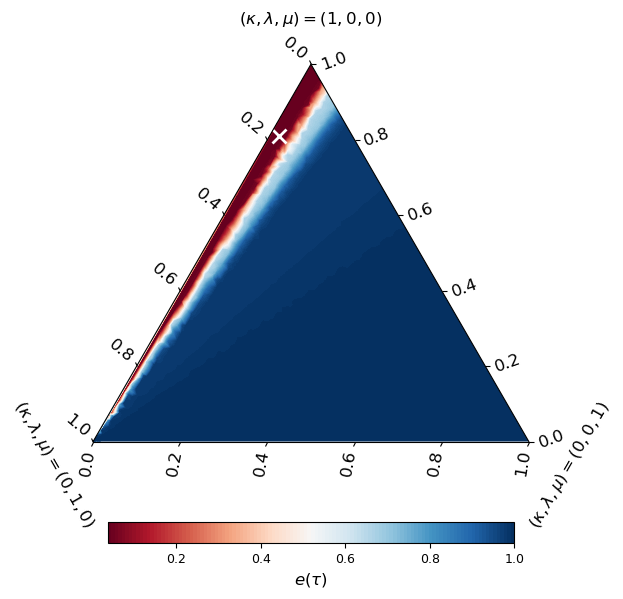
Figure 2: Effect of $\lambda$ for the STC${}_{\text{np}}$ example. The ternary plot illustrates a grid-search amongst 1000 convex combinations of $(\kappa,\lambda,\mu)$ for the ${\texttt{COTA}}{(\widehat{P})}-{\texttt{FRO}}-c_{\omega}$ setting. Values of $\lambda$ close to zero present high abstraction error, demonstrating the benefit of the do-calculus constraints in the OT problem. The minimum is reached at (.81, .17, .02) and is denoted with "$\bm{\times}$".

Method	$\mathcal{D}$	$\mathcal{C}$	$e_{{\texttt{JSD}}}(\tau)$	$e_{{\texttt{WASS}}}(\tau)$
COTA($\widehat{\tau}$)	FRO	$c_{\omega}$	$0.249\pm 0.005$	$0.135\pm 0.001$
		$c_{\mathcal{H}}$	$\bm{0.229\pm 0.003}$	$0.129\pm 0.001$

Table 2: Abstraction error for the STC${}_{\text{p}}$ example with $\mathcal{I}=\{\operatorname{do}(\operatorname{T}=0),\operatorname{do}(\operatorname{T}=1)\}$. Cost $c_{\mathcal{H}}$ outperforms $c_{\omega}$ due to limited intervention set $\mathcal{I}$.

Method	$\mathcal{D}$	$\mathcal{C}$	$e_{{\texttt{JSD}}}(\tau)$	$e_{{\texttt{WASS}}}(\tau)$
COTA($\widehat{\tau}$)	FRO	$c_{\omega}$	$0.379$	$0.053$
		$c_{\mathcal{H}}$	$\bm{0.220}$	$0.053$

Table 3: Abstraction error for the EBM example. The conventional cost $c_{\mathcal{H}}$ outperforms $c_{\omega}$ due to a limited intervention set $\mathcal{I}$.

LUng CAncer Set (LUCAS)

This model is a large-scale synthetic SCM designed to simulate data related to the study of lung cancer. Table 5 confirms that even on larger and more realistic problems COTA exceeds the baselines in terms of the abstraction error, and $c_{\omega}$ provides results at least as good as $c_{\mathcal{H}}$. The full table of results can be found in Appendix E.

Electric Battery Manufacturing (EBM)

Finally we compare with the only real-world public dataset that, to the best of our knowledge, has been used for CA learning (Zennaro et al., 2023). This dataset contains data related to electric battery manufacturing collected from two experimental settings. The first setting (WMG) has been modelled through a low-level SCM that captures the effect of a control variable (comma gap) on an output (mass loading) at multiple spatial locations. The second setting (LRCS) is modelled through a high-level SCM that relates the same control variable to a single output (Cunha et al., 2020). We learn an abstraction map $\tau$ using the set of real interventions performed during the collection of the data. Following Zennaro et al. (2023), we use the learned map $\tau$ to abstract the WMG data and aggregate them with the LRCS data; then we perform a set of downstream regression tasks. Compared to the SOTA which required full knowledge of the underlying SCM, COTA requires only knowledge of the underlying DAG and provides better results in terms of the Mean Square Error (MSE) in all the proposed setups, as shown in Table 5. In general, COTA is always the top performer compared to the baselines (see Appendix E for the complete table of results), while in Table 3 we highlight a similar behaviour as the one in Table 3 whereby the limited size of the interventional data prevents $c_{\mathcal{H}}$ to lead to better abstractions compared to $c_{\omega}$. A complete presentation of the different settings and the data of this case study can be found in Appendix D.

Method	$\mathcal{D}$	$\mathcal{C}$	$e_{{\texttt{JSD}}}(\tau)$	$e_{{\texttt{WASS}}}(\tau)$
COTA($\widehat{P}$)	FRO	$c_{\omega}$	$0.287\pm 0.014$	$\bm{0.044\pm 0.001}$
		$c_{\mathcal{H}}$	$0.287\pm 0.014$	$0.047\pm 0.001$
COTA($\widehat{\tau}$)	FRO	$c_{\omega}$	$\bm{0.263\pm 0.005}$	$0.061\pm 0.001$
		$c_{\mathcal{H}}$	$\bm{0.263\pm 0.006}$	$0.061\pm 0.001$
Pwise OT	–	$c_{\omega}$	$0.306\pm 0.009$	$0.045\pm 0.001$
	–	$c_{\mathcal{H}}$	$0.387\pm 0.002$	$0.047\pm 0.001$
Map OT	–	$c_{\omega}$	$0.294\pm 0.008$	$0.054\pm 0.001$
	–	$c_{\mathcal{H}}$	$0.350\pm 0.005$	$0.054\pm 0.001$
Bary OT	–	$c_{\omega}$	$0.294\pm 0.047$	$0.044\pm 0.003$
	–	$c_{\mathcal{H}}$	$0.414\pm 0.040$	$0.046\pm 0.010$

Table 4: Abstraction error for LUCAS. The configuration ${\texttt{COTA}}{(\widehat{\tau})}-{\texttt{FRO}}$ yields the lowest abstraction error for the JSD metric and the ${\texttt{COTA}}{(\widehat{P})}-{\texttt{FRO}}-c_{\omega}$ setting for the WASS metric. The $\omega$-cost $c_{\omega}$ outperforms $c_{\mathcal{H}}$ .

Training set	Test set	Zennaro et al. (2023)	COTA
LRCS[$CG\neq k$]	LRCS[$CG=k$]	$1.86\pm 1.75$	$1.40\pm 1.39$
LRCS[$CG\neq k$]	LRCS[$CG=k$]	$0.22\pm 0.26$	$0.19\pm 0.04$
+WMG
LRCS[$CG\neq k$]	LRCS[$CG=k$]	$1.22\pm 0.95$	$0.80\pm 0.55$
+WMG[$CG\neq k$]	WMG[$CG=k$]

Table 5: MSE of COTA and a SOTA CA framework on a regression task for EBM. Augmenting data via the learned abstraction reduces the average error in all different settings compared to the SOTA. We used ${\texttt{COTA}}{(\widehat{P})}-{\texttt{FRO}}-c_{\omega}$ with the hyperparameters $(\kappa,\lambda,\mu)=(.2,.5,.3)$ achieving the lowest abstraction error.

7 Discussion

In this work, we presented COTA, a framework for learning causal abstractions from observational and interventional data through a causally constrained multi-marginal OT formulation. Incorporating do-calculus constraints and a causally-informed cost $c_{\omega}$ in the optimisation problem led to lower abstraction error compared to non-causal baselines in diverse scenarios. The effectiveness of the $c_{\omega}$ cost was shown to be sensitive to the intervention set; expanding the interventions set improved the performance with the $\omega$-cost compared to conventional non-causal costs like Hamming. Lastly, COTA outperform the prior CA learning art of Zennaro et al. (2023) when employed as a data augmentation procedure on a real world regression task.

Our work opens up new challenges and directions in both fields of causal abstraction learning and OT. First, constrained multi-marginal OT settings like COTA have been understudied in the literature, and further theoretical work on the guarantees of existence and uniqueness of the estimated maps is needed. Recent methods for joint learning of plans and parameterised maps (Uscidda and Cuturi, 2023; Seguy et al., 2018) to obtain better estimators (Perrot et al., 2016) hold promise in this front. Furthermore, generalising a framework like COTA to semi-Markovian SCMs presents a significant challenge, because lifting the causal sufficiency assumption may render the estimation of certain causal constraints unidentifiable. Finally, another interesting direction would be to extend CA learning frameworks like COTA in order to incorporate temporal dependencies and continuous-time models, for example structural dynamical causal models (Bongers et al., 2018).

Appendix

Appendix A Derivation of normalizing vectors

We follow the notation introduced in the main text. For $\iota\preceq\eta$, $\iota=\operatorname{do}(\mathbf{A}=\mathbf{a})$ and $\omega(\iota)=\operatorname{do}(\mathbf{A}^{\prime}=\mathbf{a}^{\prime})$ induce a transport plan $P^{\iota}$, while $\eta=\operatorname{do}(\mathbf{B}=\mathbf{b})$ and $\omega(\eta)=\operatorname{do}(\mathbf{B}^{\prime}=\mathbf{b}^{\prime})$ induce a transport plan $P^{\eta}$. Our aim is to express the normalizing vectors $\mathcal{Z}^{\eta}=\mathbb{P}_{\mathcal{M}}(\mathbf{B}_{i}=\mathbf{b}_{i}\mid\operatorname{PA}(\mathbf{B}_{i}))$ and $\mathcal{Z}^{\omega(\eta)}=\mathbb{P}_{\mathcal{M}^{\prime}}(\mathbf{B^{\prime}}_{i}=\mathbf{b^{\prime}}_{i}\mid\operatorname{PA}(\mathbf{B^{\prime}}_{i}))$ in terms of the plan $P^{\iota}$. These are the conditional probabilities defined in Eq. 7 and can be written as:

$$\mathbb{P}_{\mathcal{M}}(\mathbf{B}_{i}=\mathbf{b}_{i}\mid\operatorname{PA}(\mathbf{B}_{i}))=\frac{\mathbb{P}_{\mathcal{M}}(\mathbf{B}_{i}=\mathbf{b}_{i},\operatorname{PA}(\mathbf{B}_{i}))}{\mathbb{P}_{\mathcal{M}}(\operatorname{PA}(\mathbf{B}_{i}))}~{}~{}\Bigg{\}}\text{ Base}$$ (13)

$$\mathbb{P}_{\mathcal{M}^{\prime}}(\mathbf{B^{\prime}}_{i}=\mathbf{b^{\prime}}_{i}\mid\operatorname{PA}(\mathbf{B^{\prime}}_{i}))=\frac{\mathbb{P}_{\mathcal{M}^{\prime}}(\mathbf{B^{\prime}}_{i}=\mathbf{b^{\prime}}_{i},\operatorname{PA}(\mathbf{B^{\prime}}_{i}))}{\mathbb{P}_{\mathcal{M}^{\prime}}(\operatorname{PA}(\mathbf{B^{\prime}}_{i}))}~{}~{}\Bigg{\}}\text{ Abstracted}$$ (14)

Then given $P^{\iota}\preceq P^{\eta}$ we express the sub-parts of the equations above in terms of the transportation plan $P^{\iota}$ by defining specific sets of indices on it. Starting from Eq. 13 and the denominator $\mathbb{P}_{\mathcal{M}}(\operatorname{PA}(\mathbf{B}_{i}))$, this can be then written as:

$$\mathbb{P}_{\mathcal{M}}(\operatorname{PA}(\mathbf{B}_{i}))=\sum_{[i,j]\in\mathcal{O}_{\iota,\eta,\rho}}P_{ij}^{\iota},$$ (15)

where $\mathcal{O}_{\iota,\eta,\rho}=\left\{[i,j]~{}\mid~{}x_{j}\in\operatorname{dom}[\mathbf{X}]\land\operatorname{Cmp}(x_{j},\operatorname{do}(\operatorname{PA}_{\mathbf{B}}=\rho))\right\},~{}\text{for }\rho\in\operatorname{dom}[\operatorname{PA}_{\mathbf{B}}]$.

Consequently, for the numerator we first define the following set:

$$\mathcal{C}_{\iota,\eta}=\left\{[i,j]~{}\mid~{}x_{j}\in\operatorname{dom}[\mathbf{X}]\land\operatorname{Cmp}(x_{j},\eta)\right\}$$

and also let the intersection set $\Omega_{\iota,\eta,\rho}=\mathcal{C}_{\iota,\eta}\cap\mathcal{O}_{\iota,\eta,\rho}$ for every $\rho\in\operatorname{dom}[\operatorname{PA}_{\mathbf{B}}]$. Then, we have:

$$\mathbb{P}_{\mathcal{M}}(\mathbf{B}_{i}=\mathbf{b}_{i},\operatorname{PA}(\mathbf{B}_{i}))=\sum_{[i,j]\in\Omega_{\iota,\eta,\rho}}P^{\iota}_{i,j}$$ (16)

By performing the symmetric operations for the abstracted model in Eq. 14 and get the respective sets $\mathcal{O}^{\prime}_{\iota,\eta,\rho^{\prime}},\mathcal{C}^{\prime}_{\iota,\eta}$ and $\Omega^{\prime}_{\iota,\eta,\rho}$ we can then finally define the normalizing vectors in terms of the plan as follows:

$$\mathcal{Z}^{\eta}=\frac{\sum_{[i,j]\in\Omega_{\iota,\eta,\rho}}P^{\iota}_{i,j}}{\sum_{[i,j]\in\mathcal{O}_{\iota,\eta,\rho}}P^{\iota}_{i,j}},~{}~{}\mathcal{Z}^{\omega(\eta)}=\frac{\sum_{[i,j]\in\Omega^{\prime}_{\iota,\eta,\rho}}P^{\iota}_{i,j}}{\sum_{[i,j]\in\mathcal{O}^{\prime}_{\iota,\eta,\rho^{\prime}}}P^{\iota}_{i,j}}$$ (17)

We also present the derivation of the special case in which the intervened variables have no parents. Specifically, one can easily see that in this case:

$$\mathcal{O}_{\iota,\eta,\rho}=\left\{[i,j]~{}\mid~{}x_{j}\in\operatorname{dom}[\mathbf{X}]\right\}~{}~{}\text{for }\rho\in\operatorname{dom}[\operatorname{PA}_{\mathbf{B}}]$$

$$\mathcal{O}^{\prime}_{\iota,\eta,\rho^{\prime}}=\left\{[i,j]~{}\mid~{}x^{\prime}_{i}\in\operatorname{dom}[\mathbf{X^{\prime}}]\right\}~{}~{}\text{for }\rho^{\prime}\in\operatorname{dom}[\operatorname{PA}_{\mathbf{B^{\prime}}}]$$

This implies that $\Omega_{\iota,\eta,\rho}=\mathcal{C}_{\iota,\eta}$ and similarly $\Omega^{\prime}_{\iota,\eta,\rho}=\mathcal{C}^{\prime}_{\iota,\eta}$. Therefore, since $\operatorname{PA}_{\mathbf{B}}=\operatorname{PA}_{\mathbf{B^{\prime}}}=\varnothing$ then $\operatorname{Cmp}(x_{j},\operatorname{do}(\operatorname{PA}_{\mathbf{B}}=\rho))~{}\forall~{}x_{j}\in\operatorname{dom}[\mathbf{X}]$ and $\operatorname{Cmp}(x^{\prime}_{i},\operatorname{do}(\operatorname{PA}_{\mathbf{B^{\prime}}}=\rho^{\prime}))~{}\forall~{}x^{\prime}_{i}\in\operatorname{dom}[\mathbf{X^{\prime}}]$, which suggest that $\sum_{[i,j]\in\mathcal{O}_{\iota,\eta,\rho}}P^{\iota}_{i,j}=\sum_{[i,j]\in\mathcal{O}^{\prime}_{\iota,\eta,\rho^{\prime}}}P^{\iota}_{i,j}=1$. Therefore, the normalizing vectors in Eq. 17 now become:

$$\mathcal{Z}^{\eta}=\sum_{[i,j]\in\mathcal{C}_{\iota,\eta}}P^{\iota}_{i,j},~{}~{}\mathcal{Z}^{\omega(\eta)}=\sum_{[i,j]\in\mathcal{C}^{\prime}_{\iota,\eta}}P^{\iota}_{i,j}$$ (18)

The later relation conveys that in the case of no parents for the intervened variable the normalizing vectors become constant vectors for each model and are not different for each of the $x_{j}\in\operatorname{dom}[\mathbf{X}]$ and $x^{\prime}_{i}\in\operatorname{dom}[\mathbf{X^{\prime}}]$ respectively, compared to the general case where we have a unique normalizing constant for each of these entries.

Appendix B Proof of Theorem 1

Let $D=\operatorname{dom}[\mathbf{X}]$ and $D^{\prime}=\operatorname{dom}[\mathbf{X}^{\prime}]$. Let $N(k)=N$ (the number of plans depends on the chain $k$) for simplicity. Hence we have $N$ plans in a particular chain $\mathcal{I}_{k}$. Also for simplicity of notation, let $P^{\iota_{n}}=P_{n}$, $C_{\omega}=C$. We show the proof for a generic chain, and it holds for any chain in the set of chains. To prove the theorem, we need to show:

1. The set $\underbrace{\mathcal{S}_{D\times D^{\prime}}\times\dots\mathcal{S}_{D\times D^{\prime}}}_{N\text{times}}=\{(P_{1},\dots,P_{N})~{}\mid~{}P_{n}\in\mathcal{S}_{D\times D^{\prime}},$ for all $k=1,\dots,N\}$, where $\mathcal{S}_{D\times D^{\prime}}$ is the set of stochastic matrices of dimension $D\times D^{\prime}$, is a convex set.

2. The constraints $\{P_{n}\in\mathcal{U}(\pi_{n}),n=1,\dots,N\}$ are convex.

3. The function $(P_{1},\dots,P_{N})\to\sum_{n=1}^{N}\kappa\cdot\Big{<}C,P_{n}\Big{>}+\bm{\lambda}^{\top}\mathcal{D}\left(P_{n};P_{n+1}\right)+\mu\cdot\mathcal{H}(P_{n})$ is jointly convex in $P_{1},\dots,P_{N}$. Denote this function by $f^{\text{COTA}}(P_{1},\dots,P_{N})$.

Point (1) is a consequence of the fact that each $P_{n}$ is in the set of stochastic matrices $\mathcal{S}_{D\times D^{\prime}}$, which is a convex set, and that the Cartesian product $\times$ preserves convexity. Point (2) follows since each $\mathcal{U}(\pi_{n})$ is a convex set (Peyré et al., 2019). To prove (3), we are going to use the following facts.

Lemma 1.

The domain of each $P_{n}$ is a convex set, and the inner product $P_{n}\to\Big{<}C,P_{n}\Big{>}$ is a convex function in $P_{n}$.

Proof: the domain of $P_{n}$ is the stochastic matrices as described in point (1) above; the inner product is a convex function in $P_{n}$ (Boyd and Vandenberghe, 2004) $\blacksquare$
Further, $\bm{\lambda}^{\top}\mathcal{D}(P_{n};P_{n+1})$ is jointly convex in the pair $(P_{n},P_{n+1})$, which the next lemma shows.

Lemma 2.

The function $(P_{n},P_{n+1})\rightarrow\bm{\lambda}^{\top}\mathcal{D}(P_{n};P_{n+1})$ is jointly convex in the pair $(P_{n},P_{n+1})$

$$\mathcal{D}(P_{n},P_{n+1})=[\delta_{n,n+1},\delta^{\prime}_{n,n+1}]^{\top}$$

Given that:

1. $P_{n},P_{n+1}$ are stochastic matrices, i.e., they belong to the set $\mathcal{S}_{D\times D^{\prime}}$.

2. $d$ is a Bregman divergence between probability vectors, which is jointly convex in both its inputs (Dhillon and Tropp, 2008).

3. $\delta(P_{n},P_{n+1})=d(P_{n}\mathbf{1},P_{n+1}\mathbf{1})$ , $\delta^{\prime}(P_{n},P_{n+1})=d(P_{n}^{\top}\mathbf{1},P_{n+1}^{\top}\mathbf{1})$ where $\mathbf{1}$ is a vector of ones of appropriate dimension. Note that $P_{n}\mathbf{1}$ and $P_{n}^{\top}\mathbf{1}$ are the marginals of $P_{n}$.

We want to prove that $\bm{\lambda}^{\top}\mathcal{D}(P_{n},P_{n+1})$ is jointly convex in $P_{n}$ and $P_{n+1}$, i.e., for $P_{n}^{\prime},P_{n+1}^{\prime}$ any stochastic matrices of the corresponding sizes and $\gamma\in[0,1]$, it holds (due also to linearity of matrix multiplication)

$$\bm{\lambda}^{\top}\mathcal{D}(\gamma P_{n}+(1-\gamma)P_{n}^{\prime},\gamma P_{n+1}+(1-\gamma)P_{n+1}^{\prime})\leq\gamma\bm{\lambda}^{\top}\mathcal{D}(P_{n},P_{n+1})+(1-\gamma)\bm{\lambda}^{\top}\mathcal{D}(P_{n}^{\prime},P_{n+1}^{\prime}).$$ (19)

It is now sufficient to prove that both $\delta(P_{n},P_{n+1}),\delta^{\prime}(P_{n},P_{n+1})$ are jointly convex in $P_{n}$ and $P_{n+1}$, and convexity of $\bm{\lambda}^{\top}\mathcal{D}(\cdot,\cdot)$ follows. We prove the result for $\delta$ and an analogous proof holds for $\delta^{\prime}$.

Expanding:

$$\delta(\gamma P_{n}+(1-\gamma)P_{n}^{\prime},\gamma P_{n+1}+(1-\gamma)P_{n+1}^{\prime})=d((\gamma P_{n}+(1-\gamma)P_{n}^{\prime})\mathbf{1},(\gamma P_{n+1}+(1-\gamma)P_{n+1}^{\prime})\mathbf{1}),$$

given that $d$ is a Bregman divergence and is jointly convex, for any probability vectors $\alpha,\alpha^{\prime},\beta,\beta^{\prime}$:

$$d(\gamma\alpha+(1-\gamma)\alpha^{\prime},\gamma\beta+(1-\gamma)\beta^{\prime})\leq\gamma d(\alpha,\beta)+(1-\gamma)d(\alpha^{\prime},\beta^{\prime})$$

Setting $\alpha=P_{n}\mathbf{1}$, $\alpha^{\prime}=P_{n}^{\prime}\mathbf{1}$, $\beta=P_{n+1}\mathbf{1}$, and $\beta^{\prime}=P_{n+1}^{\prime}\mathbf{1}$, we get (simply by linearity of matrix-vector multiplication):

$$d(\gamma P_{n}\mathbf{1}+(1-\gamma)P_{n}^{\prime}\mathbf{1},\gamma P_{n+1}\mathbf{1}+(1-\gamma)P_{n+1}^{\prime}\mathbf{1})\leq\gamma d(P_{n}\mathbf{1},P_{n+1}\mathbf{1})+(1-\gamma)d(P_{n}^{\prime}\mathbf{1},P_{n+1}^{\prime}\mathbf{1}).$$

This is equivalent to:

$$\delta(\gamma P_{n}+(1-\gamma)P_{n}^{\prime},\gamma P_{n+1}+(1-\gamma)P_{n+1}^{\prime})\leq\gamma\delta(P_{n},P_{n+1})+(1-\gamma)\delta(P_{n}^{\prime},P_{n+1}^{\prime}).$$

Thus, if $d$ is a Bregman divergence, making it therefore jointly convex in its two vector inputs, then $\delta$ is jointly convex in its two matrix inputs $P_{n}$ and $P_{n+1}$. $\blacksquare$

Now, we resort to the definition of joint convexity of a function $f:\underbrace{\mathcal{S}_{D\times D^{\prime}}\times\dots\mathcal{S}_{D\times D^{\prime}}}_{N\text{times}}\to\mathbb{R}_{\geq 0}$ in the tuple of matrices $(P_{1},\dots,P_{N})\in\mathcal{S}_{D\times D^{\prime}}\times\dots\mathcal{S}_{D\times D^{\prime}}$.
Definition 1 A function $f$ is jointly convex in $P_{1},\dots,P_{N}$ iff, for $\gamma\in[0,1]$ and the domain of $(P_{1},\dots,P_{N})$ is a convex set, it holds

$$f(\gamma P_{1}+(1-\gamma)P_{1}^{\prime},\dots,\gamma P_{N}+(1-\gamma)P_{N}^{\prime})\leq\gamma f(P_{1},\dots,P_{N})+(1-\gamma)f(P_{1}^{\prime},\dots,P_{N}^{\prime}).$$ (20)

We will show that for $f^{\text{COTA}}(P_{1},\dots,P_{N})$, joint convexity follows from convexity of the inner product in $P_{n}$ and joint convexity in the pairs $(P_{n},P_{n+1})$ of the distance.

By taking the convex combinations $\gamma P_{1}+(1-\gamma)P_{1}^{\prime},\dots,\gamma P_{N}+(1-\gamma)P_{N}^{\prime}$ and plugging it in, we get:

$$f^{\text{COTA}}(\gamma P_{1}+(1-\gamma)P_{1}^{\prime},\dots,\gamma P_{N}+(1-\gamma)P_{N}^{\prime})$$ (21)

$$=\sum_{n=1}^{N}\kappa\cdot\Big{<}C,\gamma P_{n}+(1-\gamma)P_{n}^{\prime}\Big{>}+\bm{\lambda}^{\top}\mathcal{D}(\gamma P_{n}+(1-\gamma)P_{n}^{\prime}~{};~{}\gamma P_{n+1}+(1-\gamma)P_{n+1}^{\prime})$$ (22)

$$+\mu\cdot\mathcal{H}(\gamma P_{n}+(1-\gamma)P_{n}^{\prime}).$$

By combining the fact that the inner product is convex in $P_{n}$ so $\Big{<}C,\gamma P_{n}+(1-\gamma)P_{n}^{\prime}\Big{>}\leq\gamma\Big{<}C,P_{n}\Big{>}+(1-\gamma)\Big{<}C,P_{n}^{\prime}\Big{>}$, the inequality from Eq. 19, and the (strict) convexity of $\mathcal{H}$, we have

$$f^{\text{COTA}}(\gamma P_{1}+(1-\gamma)P_{1}^{\prime},\dots,\gamma P_{N}+(1-\gamma)P_{N}^{\prime})$$ (23)

$$\leq\sum_{n=1}^{N}\kappa\cdot\left(\gamma\Big{<}C,P_{n}\Big{>}+(1-\gamma)\Big{<}C,P_{n}^{\prime}\Big{>}\right)+\bm{\lambda}^{\top}\left(\gamma\mathcal{D}(P_{n};P_{n+1})+(1-\gamma)\mathcal{D}(P_{n}^{\prime};P_{n+1}^{\prime})\right)$$

$$+\mu\cdot\left(\gamma\mathcal{H}(P_{n})+(1-\gamma)\mathcal{H}(P_{n}^{\prime})\right)$$

$$=\gamma\left(\sum_{n=1}^{N}\kappa\Big{<}C,P_{n}\Big{>}+\lambda\mathcal{D}(P_{n};P_{n+1})+\mu\mathcal{H}(P_{n})\right)+\left(1-\gamma\right)\sum_{n=1}^{N}\kappa\Big{<}C,P_{n}^{\prime}\Big{>}+\bm{\lambda}^{\top}\mathcal{D}(P_{n}^{\prime};P_{n+1}^{\prime})+\mu\mathcal{H}(P_{n}^{\prime})$$

$$=\gamma f^{\text{COTA}}(P_{1},\dots,P_{N})+(1-\gamma)f^{\text{COTA}}(P_{1}^{\prime},\dots,P_{N}^{\prime})$$

which is the definition of convexity in $P_{1},\dots,P_{N}$.$\blacksquare$

Appendix C OT costs

In this section we discuss the mechanics underlying the computations of the OT costs. First, we recall the $\omega$-cost function formula as it is introduced in the Eq. 11. Given two samples $\mathbf{x}\in\operatorname{dom}[\mathbf{X}]$ and $\mathbf{x}^{\prime}\in\operatorname{dom}[\mathbf{X}^{\prime}]$, and an intervention set $\mathcal{I}$ together with $\omega:\mathcal{I}\to\mathcal{I}^{\prime}$, we define the $\omega$-cost as the following function:

$$c_{\displaystyle\omega}(\mathbf{x},\mathbf{x}^{\prime})=\left|\mathcal{I}\right|-\sum\nolimits_{\iota\in\mathcal{I}}\mathbbm{1}\left[\operatorname{Cmp}(\mathbf{x},\iota)\wedge\operatorname{Cmp}(\mathbf{x}^{\prime},\omega(\iota))\right]$$

The function $c_{\omega}$ discounts the cost of transporting samples $\mathbf{x}$ to $\mathbf{x^{\prime}}$ proportionally to the number of pairs $(\iota,\omega(\iota))$ w.r.t. which $\mathbf{x}$ and $\mathbf{x^{\prime}}$ are compatible. In Fig. 3 we visualise the construction of the cost matrix $C_{\omega}$ based on the $c_{\omega}(\cdot,\cdot)$ function of Eq. 11.

As shown in Section 6, for $c_{\omega}$ to be an effective cost function, the intervention set needs to be well-specified and informative regarding the domains of the two models. In such a case, a meaningful cost matrix can be derived and more elements on the induced transport plans will be influenced by causal knowledge. Our experiments confirmed that in scenarios where the intervention set was limited, conventional costs like Hamming $c_{\mathcal{H}}$ could return lower abstraction errors compared to $c_{\omega}$. The reason is that, by construction, $c_{\omega}$ will assign maximum values $(|\mathcal{I}|)$ for samples for which it has no available information from the $\omega$ map. On the other hand, costs like $c_{\mathcal{H}}$ which spreads its values across the whole domain might be able to capture certain patterns more efficiently. We provide a visualization of the cost matrices for both $c_{\omega}$ and $c_{\mathcal{H}}$ functions in Fig. 4 and Fig. 5 respectively.

Figure 3: $\omega$-informed cost matrix computer with $|\mathcal{I}|=3$. Notice, how all values $\mathbf{x}$ and $\mathbf{x}^{\prime}$ are compatible with $\iota_{1}$ and $\omega(\iota_{1})$, while only $\mathbf{x}_{1},\mathbf{x}_{2}$ are compatible with $\operatorname{do}(\mathbf{X}[1]=0,\mathbf{X}[2]=0)$ and $\mathbf{x}^{\prime}_{1}$ is compatible with $\operatorname{do}(\mathbf{X}^{\prime}[1]=0)$

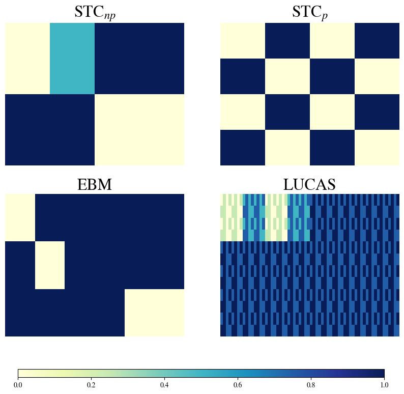
Figure 4: Omega Cost ($C_{\omega}$)

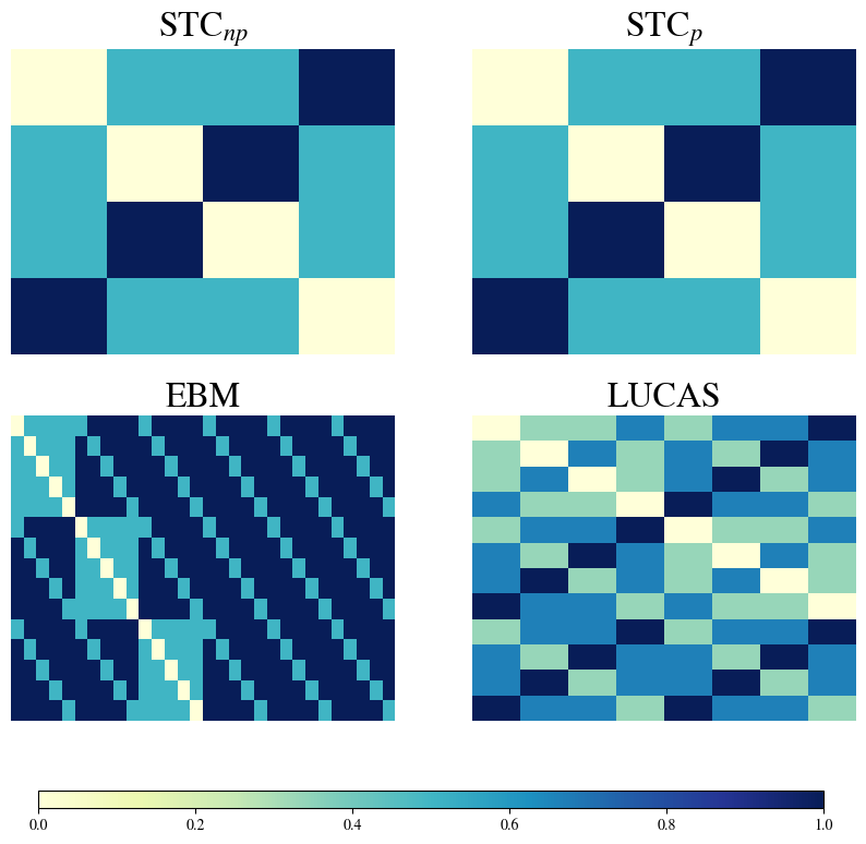
Figure 5: Hamming cost ($C_{\mathcal{H}}$)

Appendix D EBM Downstream Task

In our EBM scenario we rely on data about battery coating released by the Laboratoire de Réactivité et Chimie des Solides (LRCS) (Cunha et al., 2020) and by the Warwick Manufacturing Group (WMG) (Zennaro et al., 2023). These datasets contain observations about different variables affecting the coating process (Comma Gap, Mass Loading Position), as well as observation about a key outcome variable related to the width of the coating (Mass Loading). Both groups aim at inferring a machine learning model that would allow them to control the target variable via interventions on the other variables.

Closely following Zennaro et al. (2023), we learn abstractions from the WMG model to the LRCS model in order to merge data collected by the two laboratories and learn a model from the aggregate dataset. We compare our approach COTA with the competing CA learning method proposed in (Zennaro et al., 2023). The latter builds upon the $\mathbf{\alpha}$-abstraction framework established by Rischel (2020), which is briefly summarized in Section D.1. To assess the usefulness of abstraction, we solve three extrapolation tasks meant to show how fitting a simple model to the aggregated dataset produced via abstraction guarantees better predictive results. We consider the following three downstream tasks:

• In the first task, we train a regression model on all LRCS samples except for samples belonging to class $k$. We then test the regression model on LRCS samples belonging to class $k$. This constitutes the baseline model learned on data from a single laboratory.

• In the second task, we train a regression model on all LRCS samples except for samples belonging to class $k$ and all the abstracted WMG samples. We then test the regression model on LRCS samples belonging to class $k$. This constitutes a scenario in which we enrich one dataset (LRCS) with data from another laboratory (WMG); moreover, the enriching data provides information on the class $k$ which was not originally observerd in LRCS.

• In the third task, we train a regression model on all LRCS and abstracted WMG samples except for samples belonging to class $k$. We then test the regression model on LRCS and WMG samples belonging to class $k$. This constitutes a scenario in which we enrich one dataset (LRCS) with data from another laboratory (WMG); however, the enriching data also lacks observations for the class $k$.

Our solution outperforms the SOTA in terms of MSE, and confirms that using abstractions to aggregate data may be beneficial for downstream tasks, such as regression tasks. This is particularly true in settings where data are limited because of the cost and complexity of collecting samples, such as in the case of battery manufacturing Niri et al. (2022).

D.1 The $\mathbf{\alpha}$-abstraction framework

This framework draws inspiration from category theory, and assumes two SCMs $\mathcal{M}=\langle\mathbf{X},\mathbf{U},\mathcal{F},\mathbb{P}(\mathbf{U})\rangle$, $\mathcal{M}^{\prime}=\langle\mathbf{X^{\prime}},\mathbf{U^{\prime}},\mathcal{F}^{\prime},\mathbb{P}^{\prime}(\mathbf{U^{\prime}})\rangle$ with finite sets of endogenous variables, where each variable defined on a finite and discrete domain.

Definition 8 (Rischel (2020)).

Given two SCMs $\mathcal{M}$ and $\mathcal{M}^{\prime}$, an abstraction $\mathbf{\alpha}$ is a tuple $\left<R,a,\mathbf{\alpha}\right>$ where:

• $R\subseteq\mathbf{X}$ is a subset of relevant variables in the model $\mathcal{M}$.

• $a:R\to\mathbf{X^{\prime}}$ is a surjective map between variables, from nodes in $\mathcal{M}$ to nodes in $\mathcal{M}^{\prime}$.

• $\mathbf{\alpha}$ is a collection of surjective maps $\alpha_{X^{\prime}}:\operatorname{dom}[a^{-1}(X^{\prime})]\to\operatorname{dom}[X^{\prime}]$ where $X\subseteq\mathbf{X}$ and $X^{\prime}\subseteq\mathbf{X^{\prime}}$.

An $\mathbf{\alpha}$-abstraction establishes an asymmetric relation from a base model $\mathcal{M}$ to an abstracted model $\mathcal{M}^{\prime}$. This definition encodes a mapping on two layers: on a structural or graphical level between the nodes of the DAGs via $a$, and on a distributional level via the maps $\alpha_{X^{\prime}}$.

Rischel (2020) introduces a notion of interventional consistency between base and abstracted model, whereby interventional distributions produced in the base and abstracted model are related via the abstraction $\mathbf{\alpha}$; furthermore, a notion of abstraction error, analogous to the one used in this paper, is also proposed. It is then immediate to relate the $\tau$-abstraction and $\alpha$-abstraction as they both imply comparing distributions generated by base and abstracted model through an abstraction map.

Appendix E Additional Experiments and Analysis

Here we report the complete experimental results of our simulations. These results corroborate our understanding of the effectiveness of COTA compared to the baseline methods. Regarding the parameter $\bm{\lambda}^{\top}$, in Section E.1 we demonstrate the complete results from the the equal weight case where $\lambda=\lambda^{\prime}$ and in Section E.2 from the more general case of $\lambda\neq\lambda^{\prime}$. Notice, that throughout the results, how in STC${}_{\text{np}}$ and LUCAS $\omega$-cost $c_{\omega}$ returns lower abstraction errors compared to Hamming $c_{\mathcal{H}}$, whereas in STC${}_{\text{p}}$ and EBM the opposite holds true due to the smaller and less diverse intervention sets, as discussed in the main text and in Appendix C.

E.1 Equal weights $(\lambda=\lambda^{\prime})$.

We present the evaluation results in the case where the parameter $\bm{\lambda}^{\top}$ governing the causal constraint term in the COTA optimization objective of Eq. 12 is a constant vector i.e. $\bm{\lambda}^{\top}\cdot\mathcal{D}(P^{\iota},P^{\eta})=[\lambda,\lambda]\cdot\begin{bmatrix}\delta_{\iota,\eta}\\ \delta^{\prime}_{\iota,\eta}\end{bmatrix}=\lambda\cdot(\delta_{\iota,\eta}+\delta_{\iota,\eta}^{\prime})$. The complete evaluation for the STC examples is detailed in Table 7 and Table 9, while results for the LUCAS and the EBM examples are presented in Table 11 and Table 13 respectively.

E.2 Different weights $(\lambda\neq\lambda^{\prime})$.

We present the evaluation results in the case where the parameter $\bm{\lambda}^{\top}$ governing the causal constraint term in the COTA optimization objective of Eq. 12 is a non-constant vector i.e. $\bm{\lambda}^{\top}\cdot\mathcal{D}(P^{\iota},P^{\eta})=\left[\lambda~{}~{}\lambda^{\prime}\right]\cdot\begin{bmatrix}\delta_{\iota,\eta}\\ \delta^{\prime}_{\iota,\eta}\end{bmatrix}=\lambda\cdot\delta_{\iota,\eta}+\lambda^{\prime}\cdot\delta_{\iota,\eta}^{\prime}$. The complete evaluation for the STC examples is detailed in Table 7 and Table 9, while results for the LUCAS and the EBM examples are presented in Table 11 and Table 13, respectively. Finally, Table 14 demonstrates the MSE of COTA and a SOTA CA framework on a regression task for EBM.

Appendix F Approximate COTA

We can simplify the optimization problem and halve the number of constraints by assuming that the elements of each marginal of the plan inherit the marginal’s normalising factor (Occam’s razor). This way, we turn $\delta_{\iota,\eta}$ and $\delta^{\prime}_{\iota,\eta}$ into the element-wise (between the plans) distances $d\left(\left(\frac{1}{\mathcal{Z}^{\eta}_{j}}P^{\iota}_{ij}\right)_{ij},\left(P^{\eta}_{ij}\right)_{ij}\right)$ and $d\left(\left(\frac{1}{\mathcal{Z}^{\omega(\eta)}_{i}}P^{\iota}_{ij}\right)_{ij},\left(P^{\eta}_{ij}\right)_{ij}\right)$, respectively. Now every pair of elements $P^{\iota}_{ij},P^{\eta}_{ij}$ is related simultaneously through $\mathcal{Z}^{\eta}_{j}$ and $\mathcal{Z}^{\omega(\eta)}_{i}$. Then given $d:\mathbb{R}^{D\times D^{\prime}}\times\mathbb{R}^{D\times D^{\prime}}\to\mathbb{R}_{\geq 0}$, we re-express our constraints in a matrix form as:

$$\mathcal{D}(P^{\iota},P^{\eta})=d\left(\frac{1}{\varphi(\mathcal{Z}^{\eta}_{j},\mathcal{Z}^{\omega(\eta)}_{i})}P^{\iota},P^{\eta}\right)\quad\text{ if }\operatorname{Cmp}(x_{j},\eta)\text{ and }\operatorname{Cmp}(x_{i}^{\prime},\omega(\eta))$$ (24)

where $\varphi(\cdot,\cdot):\mathbb{R}^{2}\rightarrow\mathbb{R}$ is any aggregating function that preserves the correct support of the plans. In our experiments we work with $\varphi(\mathcal{Z}^{\eta}_{j},\mathcal{Z}^{\omega(\eta)}_{i})=\min(\mathcal{Z}^{\eta}_{j},\mathcal{Z}^{\omega(\eta)}_{i})$. We provide the complete abstraction error evaluation results as before alongside the downstream evaluation for the Approximate COTA in Section F.1.

F.1 Approximate COTA Results

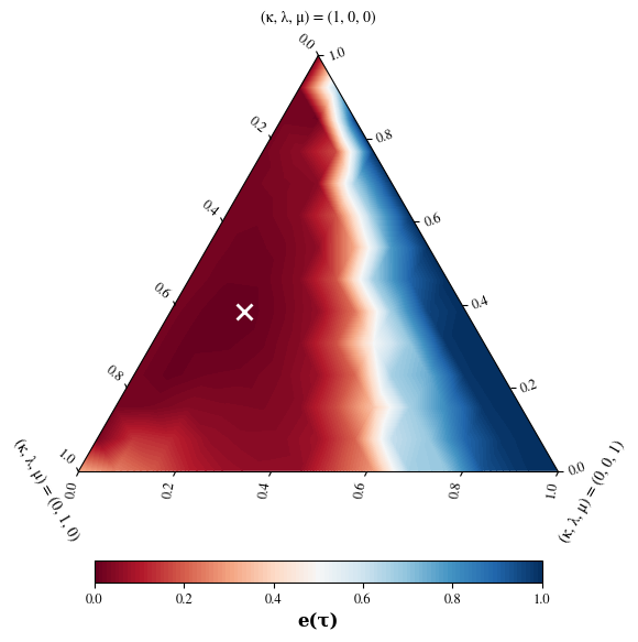
Figure 6: Effect of $\lambda$ for the STC${}_{\text{np}}$ example in the Approximate COTA formulation. The ternary plot illustrates a grid-search amongst 100 convex combinations of $(\kappa,\lambda,\mu)$ for the ${\texttt{COTA}}{(\widehat{P})}-{\texttt{FRO}}-c_{\omega}$ setting. Values of $\lambda$ close to zero present high abstraction error, demonstrating the benefit of the do-calculus constraints in the OT problem. The minimum is reached at (.38, .46, .16) and is denoted with "$\bm{\times}$"

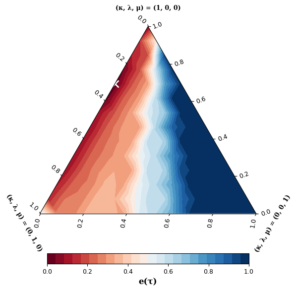
Figure 7: Effect of $\lambda$ for the STC${}_{\text{np}}$ example in the Approximate COTA formulation. The ternary plot illustrates a grid-search amongst 100 convex combinations of $(\kappa,\lambda,\mu)$ for the ${\texttt{COTA}}{(\widehat{P})}-{\texttt{JSD}}-c_{\omega}$ setting. Values of $\lambda$ close to zero present high abstraction error, demonstrating the benefit of the do-calculus constraints in the OT problem. The minimum is reached at (.61, .38, .01) and is denoted with "$\bm{\times}$"

We report the complete experimental results for Approximate COTA. Once again, we confirm our understanding of the effectiveness of COTA compared to the baseline methods. The complete evaluation for the STC examples is detailed in Table 16 and Table 16, while results for the LUCAS and the EBM examples are presented in Table 18 and Table 18, respectively. Furthermore, in STC${}_{\text{np}}$ and LUCAS $\omega$-cost $c_{\omega}$ returns lower abstraction errors compared to Hamming $c_{\mathcal{H}}$, whereas in STC${}_{\text{p}}$ and EBM the opposite holds true due to the smaller and less diverse intervention sets, as discussed in the main text and in Appendix C. In addition, in Fig. 6 and Fig. 7 we provide the equivalent simplex plots for STC${}_{\text{np}}$, which illustrate the influence of the parameter $\lambda$ in the optimization problem. Once again, these plots reinforce the idea that optimal solutions are achieved when $\lambda$ is greater than 0. Finally, in Table 19, we demonstrate the results regarding the MSE for the downstream task on the EBM dataset as before.

Method	$\mathcal{D}$	$\mathcal{C}$	$e_{{\texttt{JSD}}}(\tau)$	$e_{{\texttt{WASS}}}(\tau)$
COTA($\widehat{P}$)	FRO	$c_{\omega}$	$\bm{0.010\pm 0.005}$	$\bm{0.011\pm 0.003}$
		$c_{\mathcal{H}}$	$0.087\pm 0.007$	$0.025\pm 0.001$
	JSD	$c_{\omega}$	$0.012\pm 0.006$	$0.012\pm 0.003$
		$c_{\mathcal{H}}$	$0.087\pm 0.006$	$0.025\pm 0.001$
COTA($\widehat{\tau}$)	FRO	$c_{\omega}$	$0.013\pm 0.021$	$0.171\pm 0.001$
		$c_{\mathcal{H}}$	$0.169\pm 0.005$	$0.178\pm 0.001$
	JSD	$c_{\omega}$	$0.014\pm 0.021$	$0.171\pm 0.001$
		$c_{\mathcal{H}}$	$0.169\pm 0.004$	$0.178\pm 0.001$
Pwise OT	–	$c_{\omega}$	$0.013\pm 0.002$	$0.011\pm 0.002$
	–	$c_{\mathcal{H}}$	$0.093\pm 0.004$	$0.039\pm 0.002$
Map OT	–	$c_{\omega}$	$0.023\pm 0.022$	$0.147\pm 0.001$
	–	$c_{\mathcal{H}}$	$0.169\pm 0.022$	$0.156\pm 0.001$
Bary OT	–	$c_{\omega}$	$0.233\pm 0.142$	$0.067\pm 0.042$
	–	$c_{\mathcal{H}}$	$0.323\pm 0.074$	$0.095\pm 0.039$

Table 6: Complete abstraction error evaluation for the STC${}_{\text{np}}$ example of the $\lambda=\lambda^{\prime}$ case. The ${\texttt{COTA}}{(\widehat{P})}-{\texttt{FRO}}-c_{\omega}$ returns the lower abstraction error for both metrics. The $\omega$-cost $c_{\omega}$ outperforms $c_{\mathcal{H}}$.

Method	$\mathcal{D}$	$\mathcal{C}$	$e_{{\texttt{JSD}}}(\tau)$	$e_{{\texttt{WASS}}}(\tau)$
COTA($\widehat{P}$)	FRO	$c_{\omega}$	$\bm{0.010\pm 0.006}$	$\bm{0.010\pm 0.003}$
		$c_{\mathcal{H}}$	$0.087\pm 0.006$	$0.025\pm 0.001$
	JSD	$c_{\omega}$	$0.011\pm 0.006$	$0.012\pm 0.003$
		$c_{\mathcal{H}}$	$0.087\pm 0.006$	$0.025\pm 0.001$
COTA($\widehat{\tau}$)	FRO	$c_{\omega}$	$0.012\pm 0.020$	$0.171\pm 0.001$
		$c_{\mathcal{H}}$	$0.169\pm 0.004$	$0.178\pm 0.001$
	JSD	$c_{\omega}$	$0.013\pm 0.019$	$0.171\pm 0.001$
		$c_{\mathcal{H}}$	$0.169\pm 0.004$	$0.178\pm 0.001$
Pwise OT	–	$c_{\omega}$	$0.013\pm 0.002$	$0.011\pm 0.002$
	–	$c_{\mathcal{H}}$	$0.093\pm 0.004$	$0.039\pm 0.002$
Map OT	–	$c_{\omega}$	$0.023\pm 0.022$	$0.147\pm 0.001$
	–	$c_{\mathcal{H}}$	$0.169\pm 0.022$	$0.156\pm 0.001$
Bary OT	–	$c_{\omega}$	$0.233\pm 0.142$	$0.067\pm 0.042$
	–	$c_{\mathcal{H}}$	$0.323\pm 0.074$	$0.095\pm 0.039$

Table 7: Complete abstraction error evaluation for the STC${}_{\text{np}}$ example of the $\lambda\neq\lambda^{\prime}$ case. The ${\texttt{COTA}}{(\widehat{P})}-{\texttt{FRO}}-c_{\omega}$ returns the lower abstraction error for both metrics. The $\omega$-cost $c_{\omega}$ outperforms $c_{\mathcal{H}}$.

Method	$\mathcal{D}$	$\mathcal{C}$	$e_{{\texttt{JSD}}}(\tau)$	$e_{{\texttt{WASS}}}(\tau)$
COTA($\widehat{P}$)	FRO	$c_{\omega}$	$0.278\pm 0.015$	$\bm{0.048\pm 0.007}$
		$c_{\mathcal{H}}$	$0.241\pm 0.003$	$\bm{0.048\pm 0.007}$
	JSD	$c_{\omega}$	$0.258\pm 0.027$	$0.054\pm 0.003$
		$c_{\mathcal{H}}$	$0.242\pm 0.001$	$0.054\pm 0.003$
COTA($\widehat{\tau}$)	FRO	$c_{\omega}$	$0.249\pm 0.005$	$0.135\pm 0.001$
		$c_{\mathcal{H}}$	$\bm{0.229\pm 0.003}$	$0.129\pm 0.001$
	JSD	$c_{\omega}$	$0.241\pm 0.008$	$0.135\pm 0.001$
		$c_{\mathcal{H}}$	$\bm{0.229\pm 0.004}$	$0.129\pm 0.001$
Pwise OT	–	$\omega$	$0.279\pm 0.014$	$0.091\pm 0.005$
	–	$\mathcal{H}$	$0.242\pm 0.002$	$0.067\pm 0.001$
Map OT	–	$\omega$	$0.250\pm 0.005$	$0.140\pm 0.001$
	–	$\mathcal{H}$	$0.229\pm 0.004$	$0.129\pm 0.001$
Bary OT	–	$\omega$	$0.318\pm 0.205$	$0.104\pm 0.061$
	–	$\mathcal{H}$	$0.272\pm 0.212$	$0.075\pm 0.058$

Table 8: Complete abstraction error evaluation for the STC${}_{\text{p}}$ example of the $\lambda=\lambda^{\prime}$ case. The $c_{\mathcal{H}}$ settings of ${\texttt{COTA}}{(\widehat{\tau})}$ formulation return the lower abstraction error for the JSD metric and ${\texttt{COTA}}{(\widehat{P})}-{\texttt{FRO}}$ for the WASS metric. Table illustrates that $c_{\mathcal{H}}$ outperforms $c_{\omega}$ due to under-specification of the intervention set.

Method	$\mathcal{D}$	$\mathcal{C}$	$e_{{\texttt{JSD}}}(\tau)$	$e_{{\texttt{WASS}}}(\tau)$
COTA($\widehat{P}$)	FRO	$c_{\omega}$	$0.277\pm 0.018$	$\bm{0.046\pm 0.007}$
		$c_{\mathcal{H}}$	$0.241\pm 0.002$	$\bm{0.046\pm 0.007}$
	JSD	$c_{\omega}$	$0.273\pm 0.009$	$0.047\pm 0.006$
		$c_{\mathcal{H}}$	$0.241\pm 0.003$	$0.047\pm 0.006$
COTA($\widehat{\tau}$)	FRO	$c_{\omega}$	$0.249\pm 0.003$	$0.135\pm 0.004$
		$c_{\mathcal{H}}$	$\bm{0.228\pm 0.004}$	$0.129\pm 0.001$
	JSD	$c_{\omega}$	$0.247\pm 0.004$	$0.135\pm 0.004$
		$c_{\mathcal{H}}$	$\bm{0.228\pm 0.003}$	$0.129\pm 0.001$
Pwise OT	–	$\omega$	$0.279\pm 0.014$	$0.091\pm 0.005$
	–	$\mathcal{H}$	$0.242\pm 0.002$	$0.067\pm 0.001$
Map OT	–	$\omega$	$0.250\pm 0.005$	$0.140\pm 0.001$
	–	$\mathcal{H}$	$0.229\pm 0.004$	$0.129\pm 0.001$
Bary OT	–	$\omega$	$0.318\pm 0.205$	$0.104\pm 0.061$
	–	$\mathcal{H}$	$0.272\pm 0.212$	$0.075\pm 0.058$

Table 9: Complete abstraction error evaluation for the STC${}_{\text{p}}$ example of the $\lambda\neq\lambda^{\prime}$ case. The $c_{\mathcal{H}}$ settings of ${\texttt{COTA}}{(\widehat{\tau})}$ formulation return the lower abstraction error for the JSD metric and ${\texttt{COTA}}{(\widehat{P})}-{\texttt{FRO}}$ for the WASS metric. Table illustrates that $c_{\mathcal{H}}$ outperforms $c_{\omega}$ due to under-specification of the intervention set.

Method	$\mathcal{D}$	$\mathcal{C}$	$e_{{\texttt{JSD}}}(\tau)$	$e_{{\texttt{WASS}}}(\tau)$
COTA($\widehat{P}$)	FRO	$c_{\omega}$	$0.287\pm 0.014$	$\bm{0.044\pm 0.001}$
		$c_{\mathcal{H}}$	$0.287\pm 0.014$	$0.047\pm 0.001$
	JSD	$c_{\omega}$	$0.286\pm 0.014$	$0.048\pm 0.001$
		$c_{\mathcal{H}}$	$0.287\pm 0.014$	$0.048\pm 0.001$
COTA($\widehat{\tau}$)	FRO	$c_{\omega}$	$\bm{0.263\pm 0.005}$	$0.061\pm 0.001$
		$c_{\mathcal{H}}$	$\bm{0.263\pm 0.006}$	$0.061\pm 0.001$
	JSD	$c_{\omega}$	$\bm{0.263\pm 0.005}$	$0.062\pm 0.001$
		$c_{\mathcal{H}}$	$\bm{0.263\pm 0.006}$	$0.062\pm 0.001$
Pwise OT	–	$c_{\omega}$	$0.306\pm 0.009$	$0.045\pm 0.001$
	–	$c_{\mathcal{H}}$	$0.387\pm 0.002$	$0.047\pm 0.001$
Map OT	–	$c_{\omega}$	$0.294\pm 0.008$	$0.054\pm 0.001$
	–	$c_{\mathcal{H}}$	$0.350\pm 0.005$	$0.054\pm 0.001$
Bary OT	–	$c_{\omega}$	$0.294\pm 0.047$	$0.044\pm 0.003$
	–	$c_{\mathcal{H}}$	$0.414\pm 0.040$	$0.046\pm 0.010$

Table 10: Complete abstraction error evaluation for the LUCAS example of the $\lambda=\lambda^{\prime}$ case. All the settings of ${\texttt{COTA}}{(\widehat{\tau})}$ formulation return the lowest abstraction error for the JSD metric and the ${\texttt{COTA}}{(\widehat{P})}-{\texttt{FRO}}-c_{\omega}$ setting for the WASS metric. The $\omega$-cost $c_{\omega}$ outperforms $c_{\mathcal{H}}$.

Method	$\mathcal{D}$	$\mathcal{C}$	$e_{{\texttt{JSD}}}(\tau)$	$e_{{\texttt{WASS}}}(\tau)$
COTA($\widehat{P}$)	FRO	$c_{\omega}$	$0.287\pm 0.014$	$\bm{0.044\pm 0.001}$
		$c_{\mathcal{H}}$	$0.287\pm 0.014$	$0.047\pm 0.001$
	JSD	$c_{\omega}$	$0.287\pm 0.014$	$0.045\pm 0.001$
		$c_{\mathcal{H}}$	$0.287\pm 0.014$	$0.047\pm 0.001$
COTA($\widehat{\tau}$)	FRO	$c_{\omega}$	$\bm{0.263\pm 0.005}$	$0.060\pm 0.001$
		$c_{\mathcal{H}}$	$\bm{0.263\pm 0.006}$	$0.060\pm 0.002$
	JSD	$c_{\omega}$	$\bm{0.263\pm 0.005}$	$0.061\pm 0.001$
		$c_{\mathcal{H}}$	$\bm{0.263\pm 0.006}$	$0.061\pm 0.001$
Pwise OT	–	$c_{\omega}$	$0.306\pm 0.009$	$0.045\pm 0.001$
	–	$c_{\mathcal{H}}$	$0.387\pm 0.002$	$0.047\pm 0.001$
Map OT	–	$c_{\omega}$	$0.294\pm 0.008$	$0.054\pm 0.001$
	–	$c_{\mathcal{H}}$	$0.350\pm 0.005$	$0.054\pm 0.001$
Bary OT	–	$c_{\omega}$	$0.294\pm 0.047$	$0.044\pm 0.003$
	–	$c_{\mathcal{H}}$	$0.414\pm 0.040$	$0.046\pm 0.010$

Table 11: Complete abstraction error evaluation for the LUCAS example of the $\lambda\neq\lambda^{\prime}$ case. All the settings of ${\texttt{COTA}}{(\widehat{\tau})}$ formulation return the lowest abstraction error for the JSD metric and the ${\texttt{COTA}}{(\widehat{P})}-{\texttt{FRO}}-c_{\omega}$ setting for the WASS metric. The $\omega$-cost $c_{\omega}$ outperforms $c_{\mathcal{H}}$.

Method	$\mathcal{D}$	$\mathcal{C}$	$e_{{\texttt{JSD}}}(\tau)$	$e_{{\texttt{WASS}}}(\tau)$
COTA($\widehat{P}$)	FRO	$c_{\omega}$	$0.379$	$\bm{0.006}$
		$c_{\mathcal{H}}$	$0.263$	$\bm{0.006}$
	JSD	$c_{\omega}$	$0.379$	$\bm{0.006}$
		$c_{\mathcal{H}}$	$0.263$	$\bm{0.006}$
COTA($\widehat{\tau}$)	FRO	$c_{\omega}$	$0.379$	$0.053$
		$c_{\mathcal{H}}$	$\bm{0.220}$	$0.053$
	JSD	$c_{\omega}$	$0.399$	$0.053$
		$c_{\mathcal{H}}$	$0.263$	$0.053$
Pwise OT	–	$c_{\omega}$	$0.430$	$0.027$
	–	$c_{\mathcal{H}}$	$0.263$	$0.027$
Map OT	–	$c_{\omega}$	$0.408$	$0.060$
	–	$c_{\mathcal{H}}$	$0.228$	$0.053$
Bary OT	–	$c_{\omega}$	$0.530$	$0.019$
	–	$c_{\mathcal{H}}$	$0.335$	$0.023$

Table 12: Complete abstraction error evaluation for the EBM example of the $\lambda=\lambda^{\prime}$ case. The ${\texttt{COTA}}{(\widehat{\tau})}-{\texttt{FRO}}-c_{\mathcal{H}}$ formulation returns the lower abstraction error for the JSD metric and all the settings of ${\texttt{COTA}}{(\widehat{P})}$ for the WASS metric. Table illustrates that $c_{\mathcal{H}}$ outperforms $c_{\omega}$ due to under-specification of the intervention set.

Method	$\mathcal{D}$	$\mathcal{C}$	$e_{{\texttt{JSD}}}(\tau)$	$e_{{\texttt{WASS}}}(\tau)$
COTA($\widehat{P}$)	FRO	$c_{\omega}$	$0.311$	$\bm{0.006}$
		$c_{\mathcal{H}}$	$0.263$	$\bm{0.006}$
	JSD	$c_{\omega}$	$0.311$	$\bm{0.006}$
		$c_{\mathcal{H}}$	$0.263$	$\bm{0.006}$
COTA($\widehat{\tau}$)	FRO	$c_{\omega}$	$0.369$	$0.053$
		$c_{\mathcal{H}}$	$\bm{0.219}$	$0.053$
	JSD	$c_{\omega}$	$0.389$	$0.053$
		$c_{\mathcal{H}}$	$0.220$	$0.053$
Pwise OT	–	$c_{\omega}$	$0.430$	$0.027$
	–	$c_{\mathcal{H}}$	$0.263$	$0.027$
Map OT	–	$c_{\omega}$	$0.408$	$0.060$
	–	$c_{\mathcal{H}}$	$0.228$	$0.053$
Bary OT	–	$c_{\omega}$	$0.530$	$0.019$
	–	$c_{\mathcal{H}}$	$0.335$	$0.023$

Table 13: Complete abstraction error evaluation for the EBM example of the $\lambda\neq\lambda^{\prime}$ case. The ${\texttt{COTA}}{(\widehat{\tau})}-{\texttt{FRO}}-c_{\mathcal{H}}$ formulation returns the lower abstraction error for the JSD metric and all the settings of ${\texttt{COTA}}{(\widehat{P})}$ for the WASS metric. Table illustrates that $c_{\mathcal{H}}$ outperforms $c_{\omega}$ due to under-specification of the intervention set.

Training set	Test set	Zennaro et al. (2023)	COTA
LRCS[$CG\neq k$]	LRCS[$CG=k$]	$1.86\pm 1.75$	$1.40\pm 1.39$
LRCS[$CG\neq k$]	LRCS[$CG=k$]	$0.22\pm 0.26$	$0.20\pm 0.02$
+WMG
LRCS[$CG\neq k$]	LRCS[$CG=k$]	$1.22\pm 0.95$	$0.48\pm 0.23$
+WMG[$CG\neq k$]	WMG[$CG=k$]

Table 14: MSE of COTA with $\lambda\neq\lambda^{\prime}$ and a SOTA CA framework on a regression task for EBM. Augmenting data via the learned abstraction reduces the average error in all different settings compared to the SOTA. We used ${\texttt{COTA}}{(\widehat{P})}-{\texttt{FRO}}-c_{\omega}$ with the hyperparameters $(\kappa,\lambda,\mu)=(.2,.4,.3,.1)$ achieving the lowest abstraction error.

Method	$\mathcal{D}$	$\mathcal{C}$	$e_{{\texttt{JSD}}}(\tau)$	$e_{{\texttt{WASS}}}(\tau)$
COTA($\widehat{P}$)	FRO	$c_{\omega}$	$0.010\pm 0.005$	$0.010\pm 0.002$
		$c_{\mathcal{H}}$	$0.125\pm 0.003$	$0.011\pm 0.003$
	JSD	$c_{\omega}$	$\bm{0.008\pm 0.001}$	$\bm{0.009\pm 0.001}$
		$c_{\mathcal{H}}$	$0.036\pm 0.011$	$0.016\pm 0.002$
COTA($\widehat{\tau}$)	FRO	$c_{\omega}$	$0.013\pm 0.008$	$0.171\pm 0.001$
		$c_{\mathcal{H}}$	$0.096\pm 0.010$	$0.175\pm 0.001$
	JSD	$c_{\omega}$	$0.013\pm 0.007$	$0.171\pm 0.001$
		$c_{\mathcal{H}}$	$0.145\pm 0.008$	$0.175\pm 0.001$
Pwise OT	–	$c_{\omega}$	$0.013\pm 0.002$	$0.011\pm 0.002$
	–	$c_{\mathcal{H}}$	$0.093\pm 0.004$	$0.039\pm 0.002$
Map OT	–	$c_{\omega}$	$0.023\pm 0.022$	$0.147\pm 0.001$
	–	$c_{\mathcal{H}}$	$0.169\pm 0.022$	$0.156\pm 0.001$
Bary OT	–	$c_{\omega}$	$0.233\pm 0.142$	$0.067\pm 0.042$
	–	$c_{\mathcal{H}}$	$0.323\pm 0.074$	$0.095\pm 0.039$

Table 15: Approximate COTA complete abstraction error evaluation for the STC${}_{\text{np}}$ example. The ${\texttt{COTA}}{(\widehat{P})}-{\texttt{JSD}}-c_{\omega}$ setting returns the lower abstraction error for both metrics. The $\omega$-cost $c_{\omega}$ outperforms $c_{\mathcal{H}}$.

Method	$\mathcal{D}$	$\mathcal{C}$	$e_{{\texttt{JSD}}}(\tau)$	$e_{{\texttt{WASS}}}(\tau)$
COTA($\widehat{P}$)	FRO	$\omega$	$0.264\pm 0.001$	$0.064\pm 0.001$
		$\mathcal{H}$	$0.241\pm 0.003$	$0.060\pm 0.004$
	JSD	$\omega$	$0.259\pm 0.006$	$\bm{0.051\pm 0.002}$
		$\mathcal{H}$	$0.242\pm 0.001$	$\bm{0.051\pm 0.001}$
COTA($\widehat{\tau}$)	FRO	$\omega$	$0.248\pm 0.006$	$0.135\pm 0.001$
		$\mathcal{H}$	$\bm{0.227\pm 0.005}$	$0.129\pm 0.001$
	JSD	$\omega$	$0.236\pm 0.002$	$0.130\pm 0.005$
		$\mathcal{H}$	$\bm{0.229\pm 0.006}$	$0.129\pm 0.001$
Pwise OT	–	$\omega$	$0.279\pm 0.014$	$0.091\pm 0.005$
	–	$\mathcal{H}$	$0.242\pm 0.002$	$0.067\pm 0.001$
Map OT	–	$\omega$	$0.250\pm 0.005$	$0.140\pm 0.001$
	–	$\mathcal{H}$	$0.229\pm 0.004$	$0.129\pm 0.001$
Bary OT	–	$\omega$	$0.318\pm 0.205$	$0.104\pm 0.061$
	–	$\mathcal{H}$	$0.272\pm 0.212$	$0.075\pm 0.058$

Table 16: Approximate COTA complete abstraction error evaluation for the STC${}_{\text{p}}$ example. The ${\texttt{COTA}}{(\widehat{\tau})}-{\texttt{FRO}}-c_{\mathcal{H}}$ and ${\texttt{COTA}}{(\widehat{\tau})}-{\texttt{JSD}}-c_{\mathcal{H}}$ settings returns the lower abstraction errors for $e_{{\texttt{JSD}}}(\tau)$ and ${\texttt{COTA}}{(\widehat{P})}-{\texttt{FRO}}-c_{\omega}$ and ${\texttt{COTA}}{(\widehat{P})}-{\texttt{JSD}}-c_{\mathcal{H}}$ settings returns the lower abstraction errors for $e_{{\texttt{WASS}}}(\tau)$. Table illustrates that $c_{\mathcal{H}}$ outperforms $c_{\omega}$ due to under-specification of the intervention set.

Method	$\mathcal{D}$	$\mathcal{C}$	$e_{{\texttt{JSD}}}(\tau)$	$e_{{\texttt{WASS}}}(\tau)$
COTA($\widehat{P}$)	FRO	$c_{\omega}$	$\bm{0.258\pm 0.003}$	$\bm{0.044\pm 0.001}$
		$c_{\mathcal{H}}$	$0.260\pm 0.004$	$0.047\pm 0.001$
	JSD	$c_{\omega}$	$0.285\pm 0.014$	$0.045\pm 0.001$
		$c_{\mathcal{H}}$	$0.285\pm 0.014$	$0.046\pm 0.001$
COTA($\widehat{\tau}$)	FRO	$c_{\omega}$	$0.259\pm 0.006$	$0.060\pm 0.003$
		$c_{\mathcal{H}}$	$0.259\pm 0.006$	$0.060\pm 0.003$
	JSD	$c_{\omega}$	$0.260\pm 0.007$	$0.061\pm 0.001$
		$c_{\mathcal{H}}$	$0.263\pm 0.004$	$0.061\pm 0.001$
Pwise OT	–	$c_{\omega}$	$0.306\pm 0.009$	$0.045\pm 0.001$
	–	$c_{\mathcal{H}}$	$0.387\pm 0.002$	$0.047\pm 0.001$
Map OT	–	$c_{\omega}$	$0.294\pm 0.008$	$0.054\pm 0.001$
	–	$c_{\mathcal{H}}$	$0.350\pm 0.005$	$0.054\pm 0.001$
Bary OT	–	$c_{\omega}$	$0.294\pm 0.047$	$0.044\pm 0.003$
	–	$c_{\mathcal{H}}$	$0.414\pm 0.040$	$0.046\pm 0.010$

Table 17: Approximate COTA complete abstraction error evaluation for the LUCAS example. The ${\texttt{COTA}}{(\widehat{P})}-{\texttt{FRO}}-c_{\omega}$ setting returns the lower abstraction error for both metrics. The $\omega$-cost $c_{\omega}$ outperforms $c_{\mathcal{H}}$.

Method	$\mathcal{D}$	$\mathcal{C}$	$e_{{\texttt{JSD}}}(\tau)$	$e_{{\texttt{WASS}}}(\tau)$
COTA($\widehat{P}$)	FRO	$c_{\omega}$	$0.378$	$\bm{0.006}$
		$c_{\mathcal{H}}$	$0.263$	$\bm{0.006}$
	JSD	$c_{\omega}$	$0.378$	$\bm{0.006}$
		$c_{\mathcal{H}}$	$0.263$	$\bm{0.006}$
COTA($\widehat{\tau}$)	FRO	$c_{\omega}$	$0.389$	$0.053$
		$c_{\mathcal{H}}$	$\bm{0.226}$	$0.053$
	JSD	$c_{\omega}$	$0.389$	$0.053$
		$c_{\mathcal{H}}$	$\bm{0.226}$	$0.053$
Pwise OT	–	$c_{\omega}$	$0.430$	$0.027$
	–	$c_{\mathcal{H}}$	$0.263$	$0.027$
Map OT	–	$c_{\omega}$	$0.408$	$0.060$
	–	$c_{\mathcal{H}}$	$0.228$	$0.053$
Bary OT	–	$c_{\omega}$	$0.530$	$0.019$
	–	$c_{\mathcal{H}}$	$0.335$	$0.023$

Table 18: Approximate COTA complete abstraction error evaluation for the EBM example. The ${\texttt{COTA}}{(\widehat{\tau})}-{\texttt{FRO}}-c_{\mathcal{H}}$ and ${\texttt{COTA}}{(\widehat{\tau})}-{\texttt{JSD}}-c_{\mathcal{H}}$ settings returns the lower abstraction errors for $e_{{\texttt{JSD}}}(\tau)$ and ${\texttt{COTA}}{(\widehat{P})}$ for all settings returns the lower abstraction errors for $e_{{\texttt{WASS}}}(\tau)$. Table illustrates that $c_{\mathcal{H}}$ outperforms $c_{\omega}$ due to under-specification of the intervention set collected from the labs.

Training set	Test set	Zennaro et al. (2023)	COTA
LRCS[$CG\neq k$]	LRCS[$CG=k$]	$1.86\pm 1.75$	$1.40\pm 1.39$
LRCS[$CG\neq k$]	LRCS[$CG=k$]	$0.22\pm 0.26$	$0.13\pm 0.07$
+WMG
LRCS[$CG\neq k$]	LRCS[$CG=k$]	$1.22\pm 0.95$	$0.85\pm 0.81$
+WMG[$CG\neq k$]	WMG[$CG=k$]

Table 19: MSE of Approximate COTA and a SOTA CA framework on a regression task for EBM. Augmenting data via the learned abstraction reduces the average error in all different settings compared to the SOTA. We used ${\texttt{COTA}}{(\widehat{P})}-{\texttt{FRO}}-c_{\omega}$ with the hyperparameters $(\kappa,\lambda,\mu)=(.2,.5,.3)$ achieving the lowest abstraction error.

Appendix G DAGs and chains

In this section we provide the complete DAGs alongside their corresponding intervention posets and induced chains for all the scenarios that we considered and also visualise the operation of the $\omega$ map. For enhanced clarity and ease of navigation between different settings, we have included a concise table presented in Table 20. To provide further insight, the table also offers an analytical description of the interpretation of endogenous variables within each example for both the base and abstracted models.

Figure 8: Simple Lung Cancer (STC) base (top) and abstracted (bottom) DAGs alongside their equivalent posets $\mathcal{I}$ and $\mathcal{I}^{\prime}$ structure for the STC${}_{\text{np}}$ variation. The red arrows represent the $\omega:\mathcal{I}\to\mathcal{I}^{\prime}$ map.

Figure 9: Simple Lung Cancer (STC) base (top) and abstracted (bottom) DAGs alongside their equivalent posets $\mathcal{I}$ and $\mathcal{I}^{\prime}$ structure in the STC${}_{\text{p}}$ variation. The red arrows represent the $\omega:\mathcal{I}\to\mathcal{I}^{\prime}$ map.

Figure 10: (LUCAS) base (top) and abstracted (bottom) DAGs alongside their equivalent posets $\mathcal{I}$ and $\mathcal{I}^{\prime}$ structure. The red arrows represent the $\omega:\mathcal{I}\to\mathcal{I}^{\prime}$ map.

Figure 11: Electric Battery Manufacturing (EBM) base (top) and abstracted (bottom) DAGs alongside their equivalent posets $\mathcal{I}$ and $\mathcal{I}^{\prime}$ structure. The red arrows represent the $\omega:\mathcal{I}\to\mathcal{I}^{\prime}$ map.

Example	Figure	$\mathbf{X}$	$\mathbf{X^{\prime}}$
STC	Figure 8	S: Smoking,	S′: Smoking,
	Figure 9	T: Tar,	C′: Cancer
		C:Cancer
LUCAS	Figure 10	AN: Anxiety, SM: Smoking,	EN′: Environment,
		GE: Genetics, PP: Peer Pressure,	LC′: Lung Cancer,
		LC: Lung Cancer, FA: Fatigue,	GE′: Genetics
		CO: Coughing, AL: Allergy
EBM	Figure 11	CG: Comma Gap (lab 1),	CG′: Comma Gap (lab 2),
		ML1: Mass loading position 1 (lab 1),	ML′: Mass loading (lab 2)
		ML1: Mass loading position 2 (lab 1)

Table 20: Analytical interpretation of the base $\mathcal{M}$ and abstracted $\mathcal{M}^{\prime}$ model’s endogenous variables.

Appendix H Optimal Transport

Optimal Transport (OT) theory as surveyed in Villani et al. (2009); Santambrogio (2015) provides a mathematical framework for systematically mapping one probability measure $\mu$ to another $\nu$ by looking amongst the set of all possible ways to transport the mass from one source distribution to a target one and selecting the one which minimizes a cost function. The seminal work of Peyré et al. (2019) surveys computational algorithms to solve OT problems in practice. Overall, OT offers a versatile and powerful tool for tackling complex and diverse problems across various fields, from image processing to economics.

H.1 General Measures

Monge formulation

The initial problem formulation was given by Gaspard Monge (1781) and states the following: For two arbitrary measures $\mu$, $\nu$ on the Radon spaces $\mathcal{X}$ and $\mathcal{Y}$ respectively, the Monge problem seeks to find a map $T^{*}:\mathcal{X}\mapsto\mathcal{Y}$ such that:

$$T^{*}=\inf_{T}\Big{\{}\int_{\mathcal{X}}c(x,T(x))d\mu(x):T_{\#}\mu=\nu\Big{\}}$$ (25)

where $T_{\#}\mu$ is the pushforward function and $c:\mathcal{X}\times\mathcal{Y}\mapsto\mathbb{R}$ is the cost function representing the cost of moving a unit mass from a location $x$ to a location $y$. If such a $T^{*}$ exists and attains the infimum then this is called the optimal transport map.

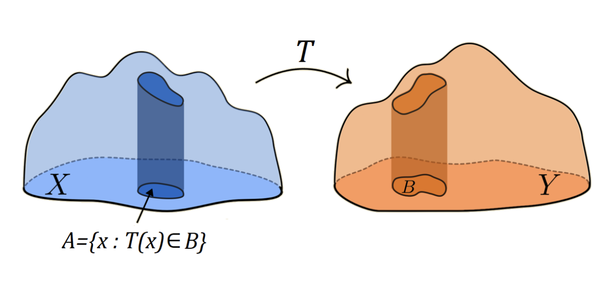
Figure 12: Monge transport map (source: (Kolouri et al., 2017) Figure 1)

Kantorovic formulation

In the initial problem formulation by Monge the map $T^{*}$ may not always exist, for example, when $\mu$ is a Dirac measure but $\nu$ is not there is no map to attain the infimum of the optimization problem above.

For this reason, Kantorovich (1942) formulation of the problem relaxes the deterministic approach of Monge and introduces the probabilistic transport idea, which allows the execution of mass splitting from a source toward several targets. Specifically, the Kantorovic problem seeks to find a joint probability measure over the space $\mathcal{X}\times\mathcal{Y}$ or probabilistic coupling, which solves the following optimization problem:

$$P^{\star}=\inf_{P}\left\{\int_{\mathcal{X}\times\mathcal{Y}}c(x,y)dP(x,y)|P\in\mathcal{U}(\mu,\nu)\right\}$$ (26)

where $\mathcal{U}(\mu,\nu)$ is the collection of all probability measures on $\mathcal{X}\times\mathcal{Y}$ with marginals $\mu$ on $\mathcal{X}$ and $\nu$ on $\mathcal{Y}$. Namely,

$$\mathcal{U}(\mu,\nu)=\big{\{}P\in\mathcal{M}_{+}^{1}(\mathcal{X}\times\mathcal{Y}):\rho_{\mathcal{X\#}}P=\mu,~{}~{}\rho_{\mathcal{Y\#}}P=\nu\big{\}}$$ (27)

where, $\rho_{\mathcal{X\#}}$ and $\rho_{\mathcal{Y\#}}$ are the pushforwards of the projections $\rho_{\mathcal{X}}(x,y)=x$ and $\rho_{\mathcal{Y}}(x,y)=y$.

This is an infinite-dimensional linear program over a space of measures. It is clear that this relaxed version of the problem is easier to work with since instead of looking for a map which that associates to each point $x_{i}\in\mathcal{X}$ a single point $y_{i}=T(x_{i})\in\mathcal{Y}$, we are looking for a probability measure with the only constraint to preserve the marginals.

The Kantorovic formulation optimal transport computes the p-Wasserstein distance metric $Wp(\cdot,\cdot)$ between two probability distributions $\mu$ and $\nu$:

$$W_{p}^{p}(\mu,\nu)=\inf_{P\in\mathcal{U}(\mu,\nu)}\int_{\mathcal{X}\times\mathcal{Y}}||x-y||^{p}dP(x,y),~{}~{}p\geq 1$$ (28)

Remarks

• Let $T$ be a transport map between $\mu$ and $\nu$, and define $P_{T}=(id,T)_{\#}\mu$. Then, $P_{T}\in\mathcal{U}(\mu,\nu)$ is a transport plan between $\mu$ and $\nu$.

• Let $\mathcal{X},\mathcal{Y}$ be two compact spaces, and $c:\mathcal{X}\times\mathcal{Y}\mapsto\mathbb{R}\cup\{+\infty\}$ be a lower semi-continuous cost function, which is bounded from below. Then Kantorovich’s problem admits a minimizer (Thorpe, 2017).

Monge–Kantorovich equivalence for general measures

The following theorem ensures that under some relatively simple conditions the Monge problem is feasible, meaning that the infimum of Eq. 25 can be attained and thus, the Kantorovich and Monge formulations are equivalent.

Theorem 2 ((Brenier, 1991)).

For Radon spaces $\mathcal{X}$ and $\mathcal{Y}$ with arbitrary measures $\mu,\nu$ respectively, if at least one of the two input measures, say $\mu$ has a density $\rho_{\mu}$ with respect to the Lebesgue measure, then there exists a unique (up to an additive constant) convex function $\phi:\mathbb{R}^{d}\mapsto\mathbb{R}$ such that $\nabla\phi$ pushes forward $\mu$ onto $\nu$. In other words, there exists a deterministic coupling $P^{\star}$ as follows:

$$dP^{\star}(x,y)=d\mu(x)\delta_{\nabla\phi(x)}(y)$$ (29)

Furthermore, if $\mathcal{X}=\mathcal{Y}=\mathbb{R}^{d}$ and $c(x,y)=||x-y||^{2}$ then the optimal $P^{\star}$ in the Kantorovic formulation is unique and is supported on the graph $(x,T(x))$ of a Monge map $T:\mathbb{R}^{d}\to\mathbb{R}^{d}$. More formally,

$$P=(id,T)_{\#\mu}\iff\forall h\in\mathcal{C}(\mathcal{X}\times\mathcal{Y}),~{}~{}\int_{\mathcal{X}\times\mathcal{Y}}h(x,y)dP(x,y)=\int_{\mathcal{X}}h(x,T(x))d\mu(x)$$ (30)

This means that the map $T$ is uniquely defined as the gradient of a unique convex function $\phi$ such that $T(x)=\nabla\phi(x)$, where $(\nabla\phi)_{\#}\mu=\nu$.

The two main conclusions from Brenier’s theorem are the following:

• In the setting of $\mathcal{W}^{2}$ with no-singular densities, the Monge problem Eq. 25 and its Kantorovich relaxation Eq. 26 are equivalent (the relaxation is tight).

• An optimal transport map (Monge map) must be the gradient of a convex function. Namely, if $\phi:\mathbb{R}^{d}\to\mathbb{R}$ convex and $(\nabla\phi)_{\#}\mu=\nu$, then $T(x)=\nabla\phi(x)$ and

  $$T^{\star}=\int_{\mathcal{X}}||x-\nabla\phi(x)||^{2}d\mu(x)$$ (31)

Various works extended the existence and uniqueness of Monge maps including strictly convex and super-linear costs.

Probabilistic interpretation

Both Monge and Kantorovich formulations can be reinterpreted through the prism of random variables (Seguy et al., 2018), Peyré et al. (2019). Consider two complete metric spaces $\mathcal{X}$ and $\mathcal{Y}$ and random variables $X$ and $Y$. We denote $X\sim\mu$ to say that $X$ is distributed according to the probability measure $\mu$. We can now restate both formulations of the optimal transport problem. Specifically, consider a cost function $c:\mathcal{X}\times\mathcal{Y}\to\mathbb{R}_{\geq 0}$ and two random variables $X\sim\mu$ and $Y\sim\nu$ taking values in $\mathcal{X}$ and $\mathcal{Y}$ respectively.

Monge formulation: Find a map $T:\mathcal{X}\to\mathcal{Y}$ which transports the mass from $\mu$ to $\nu$ while minimizing the transportation cost,

$$\inf_{T}\mathbb{E}_{X\sim\mu}\left[c(X,T_{\#\mu}(X))\right]~{}~{}\text{s.t}~{}~{}T_{\#\mu}(X)\sim Y$$ (32)

Kantorovic formulation: Find a coupling $(X,Y)\sim P$ which minimizes the transportation cost and asserts that $P$ has marginals equals to $\mu$ and $\nu$,

$$\inf_{P}\mathbb{E}_{(X,Y)\sim P}\left[c(X,Y)\right]~{}~{}\text{s.t}~{}~{}X\sim\mu,~{}~{}Y\sim\nu$$ (33)

H.2 Discrete Measures

In this section, we introduce the notations and the formulation of OT between discrete distributions. A probability vector is any element $\bm{\alpha}$ that belongs to the probability simplex $\Sigma_{k}$:

$$\Sigma_{k}:=\left\{\bm{\alpha}\in\mathbb{R}_{\geq 0}^{k}:\sum_{i=1}^{k}\alpha_{i}=1\right\}$$ (34)

A discrete measure $\mu$ with weights $\bm{\alpha}$ and points $x_{1},...,x_{k}\in\mathcal{X}\subset\mathbb{R}^{d}$ is defined as:

$$\mu=\sum_{i=1}^{k}\alpha_{i}\delta_{x_{i}}$$ (35)

where $\delta_{x}$ is the delta Dirac at position $x$. This measure is a probability measure if $\mu\in\Sigma_{k}$.

We are now going to restate the Monge-Kantorovic formulations in the cases of discrete measures. Consider $\mathcal{X}=\{x_{i}\}_{i=1}^{M}\subset\mathbb{R}^{d}$ and $\mathcal{Y}=\{y_{j}\}_{j=1}^{N}\subset\mathbb{R}^{d}$ with respective (probability) weights $\bm{\alpha}\in\Sigma_{M},\bm{\beta}\in\Sigma_{N}$. Thus, we have the discrete probability measures:

$$\mu=\sum_{i=1}^{M}\alpha_{i}\delta_{x_{i}}~{}~{}\text{and}~{}~{}\nu=\sum_{j=1}^{N}\beta_{j}\delta_{y_{j}}$$ (36)

Finally, assuming that the cost of transporting a unit of mass from $x_{i}$ to $y_{j}$ is $c(x_{i},y_{j})$ where $c:\mathcal{X}\times\mathcal{Y}\to\mathbb{R}_{\geq 0}$ is the cost function, this induces a cost matrix $C_{ij}=c(x_{i},y_{j})$.

Monge formulation for discrete measures

The Monge formulation of OT then aims to find a map $T^{\star}:\mathcal{X}\to\mathcal{Y}$ that push-forwards $\mu$ onto $\nu$, by assigning to each $x_{i}$ a single point $y_{j}$. Formally,

$$T^{\star}={\texttt{OT}}^{M}_{c}(\mu,\nu)=\operatorname*{arg\,min}_{T:~{}T_{\#}\mu=\nu}\sum_{i=1}^{M}c(x_{i},T(x_{i}))$$ (37)

Kantorovic formulation for discrete measures

Following the probabilistic transport approach of Eq. 26 for the general measures, the Kantorovich problem for discrete measures solves the following optimization problem in the form of a convex linear program:

$$P^{\star}={\texttt{OT}}^{K}_{c}(\mu,\nu)=\operatorname*{arg\,min}_{P\in\mathcal{U(\mu,\nu)}}\left<C,P\right>=\operatorname*{arg\,min}_{P\in\mathcal{U(\mu,\nu)}}\sum_{i=1,j=1}^{M,N}C_{ij}P_{ij}$$ (38)

where $\left<\cdot,\cdot\right>$ denotes the Frobenius inner product, expressing the total transportation cost, $C\in\mathbb{R}_{\geq 0}^{M\times N}$ is the cost matrix and $\mathcal{U}(\mu,\nu)$ is the set of joint probability measures with marginals $\mu$ and $\nu$ and called the transport polytope or coupling set. In particular, the transport polytope is a convex polytope defined as follows:

$$\mathcal{U}(\mu,\nu)=\left\{P\in\mathbb{R}_{\geq 0}^{M\times N}:P\mathbbm{1}_{N}=\mu,P^{\top}\mathbbm{1}_{M}=\nu\right\}=\left\{P\in\mathbb{R}^{M\times N}:\sum_{j=1}^{N}P_{ij}=\mu,~{}\sum_{i=1}^{M}P_{ij}=\nu\right\}$$ (39)

In Fig. 13 we provide a schematic viewed of input measures $(\mu,\nu)$ and a coupling $\mathcal{U}(\mu,\nu)$ encountered in the case of discrete measures for the Kantorovich OT formulation for the square euclidean cost $c(x,y)=||x-y||^{2}$.

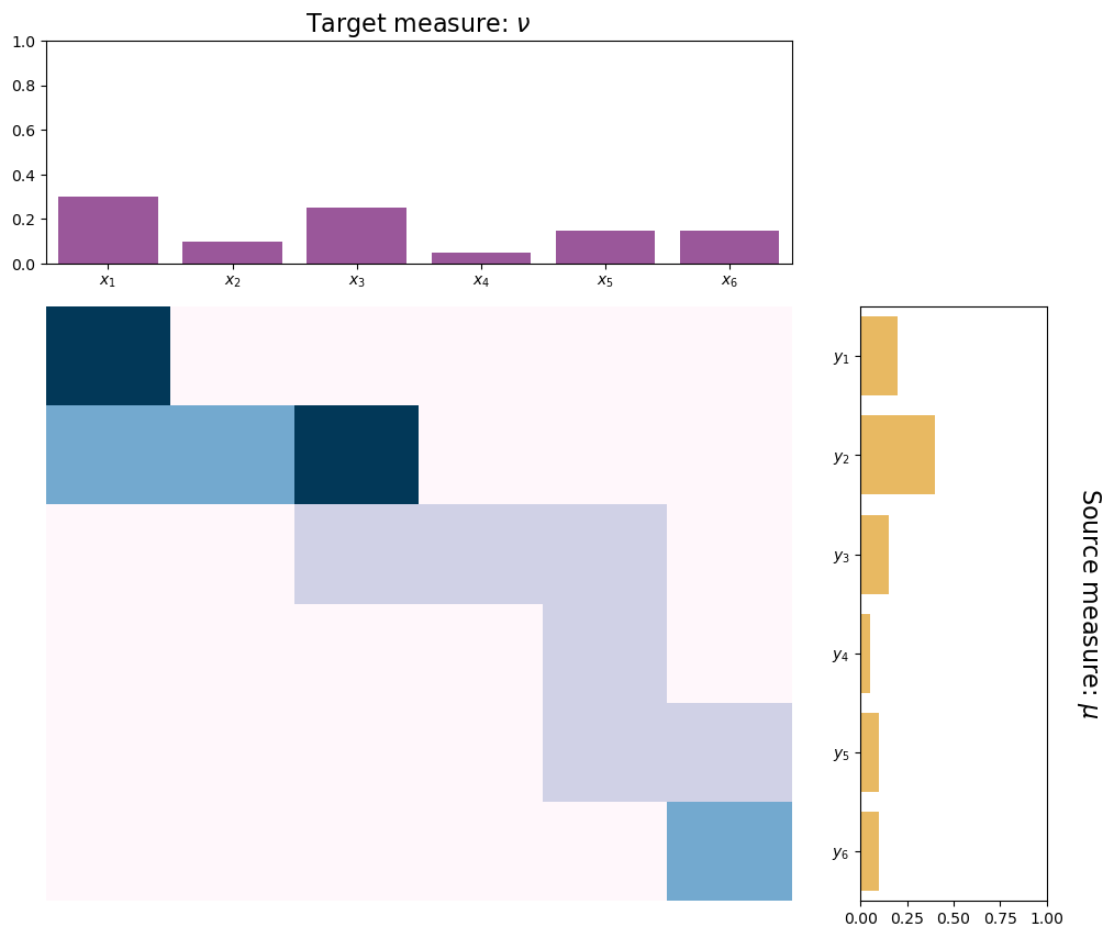
Figure 13: Kantorovic $\left({\texttt{OT}}_{c}^{K}(\mu,\nu)\right)$ optimal coupling for two input measures $\mu,\nu$. The optimal coupling $P^{\star}$ belongs to the transport polytope $\mathcal{U}(\mu,\nu)$ and thus preserves the marginals and the total mass, i.e. $\sum_{j}P^{\star}_{ij}=\mu,~{}\sum_{i}P^{\star}_{ij}=\nu$ and $\sum_{i,j}P^{\star}_{ij}=1$.

Entropic Optimal Transport

Traditional OT, while being a powerful tool, often encounters computational and statistical challenges in high-dimensional spaces. The introduction of entropy into this framework (Peyré et al., 2019) offers an organic solution that facilitates scalability and computational tractability through specific algorithms like Sinkhorn (Cuturi, 2013). Overall, Entropic OT leverages the principles of information theory, allowing for a more flexible and robust approach to the transportation problem between distributions. Specifically, for discrete measures, Entropic OT solves the following optimisation problem:

$$P^{\star}={\texttt{OT}}_{c}^{K}(\mu,\nu)_{\epsilon}=\operatorname*{arg\,min}_{P\in\mathcal{U(\mu,\nu)}}\left<C,P\right>-\epsilon\mathcal{H}(P)=\operatorname*{arg\,min}_{P\in\mathcal{U(\mu,\nu)}}\sum_{i=1,j=1}^{M,N}C_{i,j}P_{i,j}-\epsilon\mathcal{H}(P)$$ (40)

where $\epsilon>0$ a trade-off parameter and $\mathcal{H}(P)$ is the discrete entropy of a coupling matrix $P$ is defined as:

$$\mathcal{H}(P):=-\sum_{ij}P_{ij}(\log(P_{ij}-1))$$ (41)

The idea behind Entropic regularization in optimal transport involves employing a regularization function to derive approximate solutions to the original transport problem of Eq. 38.

Remarks (Peyré et al., 2019)

• ${\texttt{OT}}_{c}^{K}(\mu,\nu)_{\epsilon}\xrightarrow{\epsilon\to 0}{\texttt{OT}}_{c}^{K}(\mu,\nu)$

• ${\texttt{OT}}_{c}^{K}(\mu,\nu)_{\epsilon}\xrightarrow{\epsilon\to+\infty}\mu\otimes\nu=\mu\nu^{\top}$

Finally, it is worth mentioning that, given the strong concavity of $\mathcal{H}$, the objective in Eq. 40 becomes an $\epsilon$-strongly convex function, ensuring the optimization problem ${\texttt{OT}}_{c}^{K}(\mu,\nu)_{\epsilon}$ has a unique solution. In Fig. 14 we provide again the optimal coupling $\mathcal{U}(\mu,\nu)$ encountered in the case of discrete measures for the Entropic OT formulation for the square euclidean cost $c(x,y)=||x-y||^{2}$.

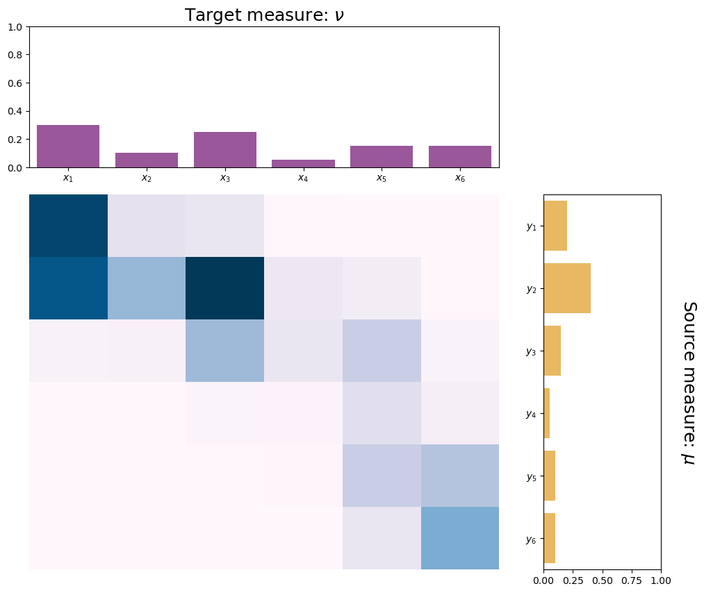
Figure 14: Kantorovic Entropic OT $\left({\texttt{OT}}_{c}^{K}(\mu,\nu)_{\epsilon}\right)$ optimal coupling for two input measures $\mu,\nu$ and $\epsilon>0$. The optimal coupling $P^{\star}$ belongs to the transport polytope $\mathcal{U}(\mu,\nu)$ and thus preserves the marginals and the total mass, i.e. $\sum_{j}P^{\star}_{ij}=\mu,~{}\sum_{i}P^{\star}_{ij}=\nu$ and $\sum_{i,j}P^{\star}_{ij}=1$.

References

- Weinan (2011) E Weinan. Principles of multiscale modeling. Cambridge University Press, 2011.
- Somnath et al. (2021) Vignesh Ram Somnath, Charlotte Bunne, and Andreas Krause. Multi-scale representation learning on proteins. Advances in Neural Information Processing Systems, 34:25244–25255, 2021.
- Geiger et al. (2021) Atticus Geiger, Hanson Lu, Thomas Icard, and Christopher Potts. Causal abstractions of neural networks. Advances in Neural Information Processing Systems, 34:9574–9586, 2021.
- Schölkopf et al. (2021) Bernhard Schölkopf, Francesco Locatello, Stefan Bauer, Nan Rosemary Ke, Nal Kalchbrenner, Anirudh Goyal, and Yoshua Bengio. Toward causal representation learning. Proceedings of the IEEE, 109(5):612–634, 2021.
- Chalupka et al. (2017) Krzysztof Chalupka, Frederick Eberhardt, and Pietro Perona. Causal feature learning: an overview. Behaviormetrika, 44(1):137–164, 2017.
- Pearl and Bareinboim (2011) Judea Pearl and Elias Bareinboim. Transportability of causal and statistical relations: A formal approach. In Proceedings of the AAAI Conference on Artificial Intelligence, volume 25, pages 247–254, 2011.
- Peters et al. (2016) Jonas Peters, Peter Bühlmann, and Nicolai Meinshausen. Causal inference by using invariant prediction: identification and confidence intervals. Journal of the Royal Statistical Society. Series B (Statistical Methodology), pages 947–1012, 2016.
- Yin et al. (2021) Mingzhang Yin, Yixin Wang, and David M Blei. Optimization-based causal estimation from heterogenous environments. arXiv preprint arXiv:2109.11990, 2021.
- Rubenstein et al. (2017) Paul K Rubenstein, Sebastian Weichwald, Stephan Bongers, Joris M Mooij, Dominik Janzing, Moritz Grosse-Wentrup, and Bernhard Schölkopf. Causal consistency of structural equation models. In 33rd Conference on Uncertainty in Artificial Intelligence (UAI 2017), pages 808–817. Curran Associates, Inc., 2017.
- Beckers and Halpern (2019) Sander Beckers and Joseph Y Halpern. Abstracting causal models. In Proceedings of the AAAI Conference on Artificial Intelligence, volume 33, pages 2678–2685, 2019.
- Rischel (2020) Eigil Fjeldgren Rischel. The category theory of causal models. Master’s thesis, University of Copenhagen, 2020.
- Massidda et al. (2022) Riccardo Massidda, Atticus Geiger, Thomas Icard, and Davide Bacciu. Causal abstraction with soft interventions. arXiv preprint arXiv:2211.12270, 2022.
- Beckers et al. (2020) Sander Beckers, Frederick Eberhardt, and Joseph Y Halpern. Approximate causal abstractions. In Uncertainty in Artificial Intelligence, pages 606–615. PMLR, 2020.
- Zennaro et al. (2023) Fabio Massimo Zennaro, Máté Drávucz, Geanina Apachitei, W. Dhammika Widanage, and Theodoros Damoulas. Jointly learning consistent causal abstractions over multiple interventional distributions. In 2nd Conference on Causal Learning and Reasoning, 2023. URL https://openreview.net/forum?id=RNs7aMS6zDq.
- Kantorovich (1942) L. Kantorovich. On the transfer of masses (in russian). Doklady Akademii Nauk, August 1942.
- Pearl (2009) Judea Pearl. Causality. Cambridge University Press, 2009.
- Peters et al. (2017) Jonas Peters, Dominik Janzing, and Bernhard Schölkopf. Elements of causal inference: Foundations and learning algorithms. MIT Press, 2017.
- Spirtes et al. (2000) Peter Spirtes, Clark N Glymour, and Richard Scheines. Causation, prediction, and search. MIT press, 2000.
- Rischel and Weichwald (2021) Eigil F Rischel and Sebastian Weichwald. Compositional abstraction error and a category of causal models. arXiv preprint arXiv:2103.15758, 2021.
- Villani et al. (2009) Cédric Villani et al. Optimal transport: old and new, volume 338. Springer, 2009.
- Peyré et al. (2019) Gabriel Peyré, Marco Cuturi, et al. Computational optimal transport: With applications to data science. Foundations and Trends® in Machine Learning, 11(5-6):355–607, 2019.
- Monge (1781) Gaspard Monge. Mémoire sur la théorie des déblais et des remblais. Mem. Math. Phys. Acad. Royale Sci., pages 666–704, 1781.
- Dhillon and Tropp (2008) Inderjit S Dhillon and Joel A Tropp. Matrix nearness problems with bregman divergences. SIAM Journal on Matrix Analysis and Applications, 29(4):1120–1146, 2008.
- Torous et al. (2021) William Torous, Florian Gunsilius, and Philippe Rigollet. An optimal transport approach to causal inference. arXiv preprint arXiv:2108.05858, 2021.
- Gunsilius and Xu (2021) Florian Gunsilius and Yuliang Xu. Matching for causal effects via multimarginal optimal transport. arXiv preprint arXiv:2112.04398, 2021.
- Tu et al. (2022) Ruibo Tu, Kun Zhang, Hedvig Kjellström, and Cheng Zhang. Optimal transport for causal discovery. In The Tenth International Conference on Learning Representations, ICLR 2022, Virtual Event, April 25-29, 2022. OpenReview.net, 2022. URL https://openreview.net/forum?id=qwBK94cP1y.
- Pass (2015) Brendan Pass. Multi-marginal optimal transport: theory and applications. ESAIM: Mathematical Modelling and Numerical Analysis-Modélisation Mathématique et Analyse Numérique, 49(6):1771–1790, 2015.
- Kostic et al. (2022) Vladimir R Kostic, Saverio Salzo, and Massimiliano Pontil. Batch greenkhorn algorithm for entropic-regularized multimarginal optimal transport: Linear rate of convergence and iteration complexity. In International Conference on Machine Learning, pages 11529–11558. PMLR, 2022.
- Cunha et al. (2020) Ricardo Pinto Cunha, Teo Lombardo, Emiliano N Primo, and Alejandro A Franco. Artificial intelligence investigation of nmc cathode manufacturing parameters interdependencies. Batteries & Supercaps, 3(1):60–67, 2020.
- Uscidda and Cuturi (2023) Théo Uscidda and Marco Cuturi. The monge gap: A regularizer to learn all transport maps. arXiv preprint arXiv:2302.04953, 2023.
- Seguy et al. (2018) Vivien Seguy, Bharath Bhushan Damodaran, Rémi Flamary, Nicolas Courty, Antoine Rolet, and Mathieu Blondel. Large scale optimal transport and mapping estimation. In 6th International Conference on Learning Representations, ICLR 2018, Vancouver, BC, Canada, April 30 - May 3, 2018, Conference Track Proceedings. OpenReview.net, 2018. URL https://openreview.net/forum?id=B1zlp1bRW.
- Perrot et al. (2016) Michaël Perrot, Nicolas Courty, Rémi Flamary, and Amaury Habrard. Mapping estimation for discrete optimal transport. Advances in Neural Information Processing Systems, 29, 2016.
- Bongers et al. (2018) Stephan Bongers, Tineke Blom, and Joris M Mooij. Causal modeling of dynamical systems. arXiv preprint arXiv:1803.08784, 2018.
- Boyd and Vandenberghe (2004) Stephen P Boyd and Lieven Vandenberghe. Convex optimization. Cambridge university press, 2004.
- Niri et al. (2022) Mona Faraji Niri, Kailong Liu, Geanina Apachitei, Luis A.A Román-Ramírez, Michael Lain, Dhammika Widanage, and James Marco. Quantifying key factors for optimised manufacturing of li-ion battery anode and cathode via artificial intelligence. Energy and AI, 7:100129, jan 2022. doi:10.1016/j.egyai.2021.100129.
- Santambrogio (2015) Filippo Santambrogio. Optimal transport for applied mathematicians. Birkäuser, NY, 55(58-63):94, 2015.
- Kolouri et al. (2017) Soheil Kolouri, Se Rim Park, Matthew Thorpe, Dejan Slepcev, and Gustavo K. Rohde. Optimal mass transport: Signal processing and machine-learning applications. IEEE Signal Processing Magazine, 34(4):43–59, 2017. doi:10.1109/MSP.2017.2695801.
- Thorpe (2017) Matthew Thorpe. Introduction to optimal transport. 2017. URL https://api.semanticscholar.org/CorpusID:131768046.
- Brenier (1991) Yann Brenier. Polar factorization and monotone rearrangement of vector-valued functions. Communications on Pure and Applied Mathematics, 44(4):375–417, 1991. doi:https://doi.org/10.1002/cpa.3160440402. URL https://onlinelibrary.wiley.com/doi/abs/10.1002/cpa.3160440402.
- Cuturi (2013) Marco Cuturi. Sinkhorn distances: Lightspeed computation of optimal transport. Advances in neural information processing systems, 26, 2013.