Classically-embedded split Cayley hexagons rule three-qubit contextuality with three-element contexts

Abstract

As it is well known, split Cayley hexagons of order two live in the three-qubit symplectic polar space in two non-isomorphic embeddings, called classical and skew. Although neither of the two embeddings yields observable-based contextual configurations of their own, classically-embedded copies are found to fully rule contextuality properties of the most prominent three-qubit contextual configurations in the following sense: each set of unsatisfiable contexts of such a contextual configuration is isomorphic to the set of lines that certain classically-embedded hexagon shares with this particular configuration. In particular, for a doily this shared set comprises three pairwise disjoint lines belonging to a grid of the doily, for an elliptic quadric the corresponding set features nine mutually disjoint lines forming a (Desarguesian) spread on the quadric, for a hyperbolic quadric the set entails 21 lines that are in bijection with the edges of the Heawood graph and, finally, for the configuration that consists of all the 315 contexts of the space its 63 unsatisfiable ones cover an entire hexagon. A particular illustration of this encoding is provided by the line-complement of a skew-embedded hexagon; its 24 unsatisfiable contexts correspond exactly to those 24 lines in which a particular classical copy of the hexagon differs from the considered skew-embedded one. In connection with the last-mentioned case we also conducted some experimental tests on a Noisy Intermediate Scale Quantum (NISQ) computer to validate our theoretical findings.

1 Introduction

Finite geometry is a branch of mathematics that deals with geometries made of a finite number of points, lines and/or linear spaces of higher dimensions. This perspective of working with spaces that contain only a finite number of geometric elements is rather counter-intuitive and far from the intuition provided, for example, by Euclidean geometry as it lacks concepts like smoothness, differentiability, distance etc. Gino Fano [fano] was one of the first geometers to formalize this idea and his name is now associated with the smallest finite projective plane, i. e. the Fano plane (Figure 1).

Figure 1: The Fano plane depicted in its standard rendering. This self-dual geometry comprises seven points (bullets) and seven lines (six straight segments and a circle), with three points per line and, dually, three lines through a point, being equivalent to the projective plane over the two-elements field $\mathbb{F}_{2}=\{0,1\}$.

Over the past 20 years (see, for example, [sp06], [hs08], [slp12], [lps13] and [ls17]), finite geometry has been introduced into the field of quantum information and mathematical physics to mainly model and analyse the commutation relations within the $n$-qubit Pauli group, $\mathcal{P}_{n}$, defined by

$$\mathcal{P}_{n}=\{sA_{1}A_{2}\dots A_{n}:A_{i}\in\{I,X,Y,Z\},s\in\{\pm 1,\pm i\}\},$$ (1)

where $A_{1}A_{2}\dots A_{n}\equiv A_{1}\otimes A_{2}\otimes\dots\otimes A_{n}$. For example, for $n=3$, if one ignores the global phase of each operator, a maximum set of mutually commuting three-qubit Pauli operators (disregarding the identity) forms a Fano plane, as shown with the example provided by Figure 2. Two points are colinear if and only if the matrix product of the observables labelling them commute.

Figure 2: The Fano plane labelled by three-qubit observables encapsulates the fact that these seven observables form a set of mutually commuting operators. In fact, it is an example of a maximal set of mutually commuting observables in the three-qubit Pauli group.

In what follows, a (quantum) context will be a set of mutually commuting observables such that their product is $\pm I^{\otimes n}$. For instance, the seven observables of Figure 2 form a (negative) three-qubit context. A contextual configuration will be an arrangement of observables made of contexts such that there is no Non-Contextual Hidden Variable (NCHV) model that can reproduce the outcomes predicted by the rules of Quantum Mechanics (QM).

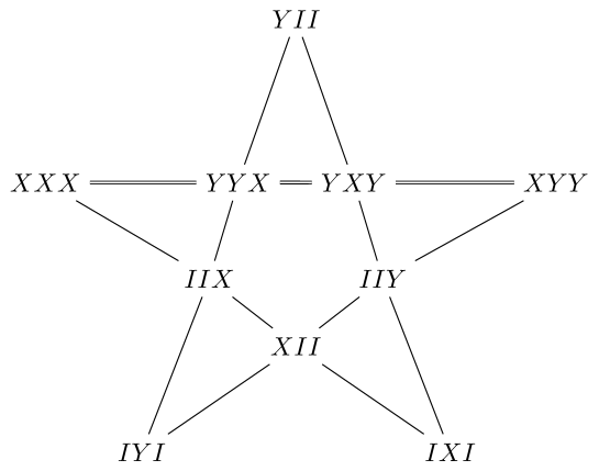
Figure 3: Mermin pentagram: This configuration of ten three-qubit observables provides an operator-based proof of the Kochen-Specker Theorem. There is no NCHV model that can reproduce the outcomes predicted by QM for this configuration.

Let us consider, for example, the configuration portrayed in Figure 3, known as the Mermin pentagram. Each node of the configuration is a three-qubit Pauli operator whose eigenvalues are $+1$ and $-1$. Each line of the configuration represents a context. The doubled line is the unique context with a negative sign, i. e. the product of the observables on this context is $-I^{\otimes 3}$. David Mermin introduced this configuration in [mermin] as an alternative proof of the famous Kochen-Specker (KS) Theorem [kochen1990problem]. Recall that the Kochen-Specker Theorem is a no-go result that proves the non-existence of an NCHV model, i. e. it proves that a Hidden Variable (HV) model that would reproduce the outcomes predicted by QM has to be context-dependent. Consider our Mermin pentagram. An HV model that reproduces predictions of QM for this set of operators should satisfy the following constraints:

1. Each node gets assigned a pre-definite measurement value $\pm 1$.

2. The product of the measurements on each context (line) should be of the same sign as the context itself.

The second constraint stems from the fact that the product of the eigenvalues of a set of mutually commuting observables should be an eigenvalue of the product of the observables. As it can readily be discerned from Figure 3, this sign constraint is not satisfiable unless the pre-definite values on the nodes are context-dependent. Note that the negative line of the Mermin pentagram of Figure 3 is nothing but the set of four mutually commuting observables one obtains from the Fano plane provided by Figure 2 by removing the (circled) line and its points.

Observable-based proof of the KS Theorem can already be built from two-qubit Pauli observables, like in the Mermin-Peres magic square, see Section 2 and  [peres1991two, mermin]. For more information on the two-qubit case, the reader is referred to consult [DHGMS22, HS17], as well as [budroni2022kochen] for a recent survey on contextuality.

In this paper we will focus solely on the three-qubit case ($n=3$) to demonstrate in detail how a specific arrangement of three-qubit contexts isomorphic to the smallest split Cayley hexagon underpins contextuality properties of a whole class of distinguished aggregates of three-qubit observables. This hexagon made its debut in physics as early as 2008 in [lsv], where the authors employed its particular three-qubit subgeometry to model the $E_{7}$-symmetric black-hole entropy formula in string theory. Later [psh], it was pointed out that the order of the automorphism group of the hexagon, 12 096, coincides with the total number of three-qubit Mermin pentagrams. At about the same time [sppl], it was already noticed that some contextual three-qubit configurations can be uniquely extended to geometric hyperplanes of the hexagon.

It is however only very recently [holweck2022three] that the fact that the hexagon embeds in the three-qubit space in two different ways has been properly taken into account and recognized as having deep physical meaning, leading to our present study.

The paper is organized as follow. In Section 2 we introduce the notion of the symplectic polar space of rank $n$ and order two, $\mathcal{W}(2n-1,2)$, which is the geometric framework for the commutation relations within the $n$-qubit generalized Pauli group. Next, we define the most prominent subgeometries of this space, quadrics, and show that the particular space $\mathcal{W}(5,2)$ for three-qubits is endowed with another remarkable kind of subgeometry, namely the split Cayley hexagon of order two, which occurs in this space in two non-isomorphic embeddings. Then we introduce the notion of the degree of contextuality of a quantum configuration, that measures how far a contextual configuration of observables is from supporting an NCHV model, and explicitly illustrate this notion on the example of the smallest symplectic space $\mathcal{W}(3,2)$, the doily, and one of its hyperbolic quadrics. Section 3 deals with the two types of hexagon’s embeddings. We first discuss the principal difference between them making use of spreads of planes. Then we show how the intersections of a skew-embedded hexagon with various doilies help us to better understand the fact that the complement of this hexagon is a contextual configuration. Section 4, the core section of the paper, first highlights the facts that the degree of contextuality of the configuration comprising all 315 line-contexts of $\mathcal{W}(5,2)$ is equal to $63$ and that the corresponding 63 unsatisfiable contexts of this configuration are the 63 lines of a copy of the split Cayley hexagon of order two that is embedded classically into $\mathcal{W}(5,2)$. The first property is then substantiated by a chain of group-theoretic and algebro-geometric arguments. After introducing a line-layered decomposition of the hexagon and describing how this decomposition helps us to quickly alternate between the two embeddings, we illustrate on several examples another crucial finding, namely that contextuality properties of most prominent families of contextual three-qubit configurations having three-element contexts, entailing doilies, elliptic quadrics and hyperbolic quadrics, are fully described in terms of their intersection with properly-selected classically-embedded copies of the hexagon. As a substantiation of our findings, Section 5 outlines the results of testing a specific contextual inequality introduced by Cabello on the IBM Quantum Experience by employing an elliptic quadric and the complement of a particular copy of skew-embedded hexagon of $\mathcal{W}(5,2)$. Our procedure follows and improves that of [holweck2021testing], where the contextuality of $\mathcal{W}(5,2)$ as a whole was already successfully tested. Finally, Section 6 summarises the main achievements and makes some proposals of how to tackle the next case, that of four qubits, in a similar unifying way.

2 Contextual configurations in symplectic polar spaces, degree of contextuality

Over the past $15$ years symplectic geometry over the two-elements field has been investigated in the context of quantum information as it encodes the commutation relations between the elements of the $n$-qubit Pauli group [saniga2007multiple, havlicek2009factor]. Recall that the Pauli matrices $X,Y,Z$ and the identity operator $I$ can be given in terms of $X$ and $Z$ as follows (phase omitted): $X=Z^{0}X,Y=Z^{1}X^{1},Z=Z^{1}X^{0}$ and $I=Z^{0}X^{0}$. Consider the map:

$$\begin{array}[]{ccc}\mathcal{P}_{n}/\{\pm I^{\otimes n},\pm iI^{\otimes n}\}&\to&\mathbb{F}_{2}^{2n}\\ (Z^{a_{1}}X^{b_{1}})\otimes(Z^{a_{2}}X^{b_{2}})\otimes\dots\otimes(Z^{a_{n}}X^{b_{n}})&\mapsto&(a_{1},a_{2},\dots,a_{n},b_{1},b_{2},\dots,b_{n}).\end{array}$$

This map associates bijectively to any $n$-qubit Pauli matrix (up to a phase) a unique vector of $\mathbb{F}_{2}^{2n}$. Thinking projectively, one can associate to any (phase disregarded) non-trivial operator of $\mathcal{P}_{n}/\{\pm I^{\otimes n},\pm iI^{\otimes n}\}$ a unique point of PG$(2n-1,2)$, the projective space over the two-elements field.

Let us equip the projective space PG$(2n-1,2)$ with the symplectic form defined as

$$\sigma(x,y)=x_{1}y_{n+1}+x_{2}y_{n+2}+\dots x_{n}y_{2n}+x_{n+1}y_{1}+x_{n+2}y_{2}+\dots+x_{2n}y_{n}.$$

Then the space $\mathcal{W}(2n-1,2)$ of all totally isotropic subspaces of PG$(2n-1,2)$ with respect to $\sigma$ is called the symplectic polar space of rank $n$ and order $2$. This space encodes the commutation relations of $\mathcal{P}_{n}$ in the sense that one can check by a straightforward calculation that any pair of isotropic elements $x,y\in\mathcal{W}(2n-1,2)$ corresponds to two commuting observables $O_{x}$ and $O_{y}$ in $\mathcal{P}_{n}$, see e. g. [havlicek2009factor].

A large number of contextual configurations can thus be advantageously identified with subgeometries of $\mathcal{W}(2n-1,2)$. Indeed, as contexts are sets of mutually commuting observables whose products are, up to a sign, equal to the identity operator, then all lines, planes, and more generally linear subspaces of $\mathcal{W}(2n-1,2)$ can be chosen as contexts. For example, the Fano plane depicted in Figure 2 is a linear subspace of the largest dimension in $\mathcal{W}(5,2)$. The most prominent subgeometries of $\mathcal{W}(2n-1,2)$ are quadrics. A hyperbolic quadric $\mathcal{Q}^{+}(2n-1,2)$, $n\geq 1$, is a subgeometry whose equation can be brought to the following standard form

$$x_{1}x_{n+1}+x_{2}x_{n+2}\ldots+x_{n}x_{2n}=0.$$ (2)

Each $\mathcal{Q}^{+}(2n-1,2)$ contains

$$|\mathcal{Q}^{+}|_{p}=(2^{n-1}+1)(2^{n}-1)$$ (3)

points and there are

$$|W|_{\mathcal{Q}^{+}}=|\mathcal{Q}^{+}|_{p}+1=(2^{n-1}+1)(2^{n}-1)+1$$ (4)

copies of them in $\mathcal{W}(2n-1,2)$. An elliptic quadric $\mathcal{Q}^{-}(2n-1,2)$, $n\geq 2$, comprises all points and subspaces of $\mathcal{W}(2n-1,2)$ satisfying the standard equation

$$f(x_{1},x_{n+1})+x_{2}x_{n+2}+\cdots+x_{n}x_{2n}=0,$$ (5)

where $f$ is an irreducible polynomial over $\mathbb{F}_{2}$. Each $\mathcal{Q}^{-}(2n-1,2)$ contains

$$|\mathcal{Q}^{-}|_{p}=(2^{n-1}-1)(2^{n}+1)$$ (6)

points and $\mathcal{W}(2n-1,2)$ features

$$|W|_{\mathcal{Q}^{-}}=|\mathcal{Q}^{-}|_{p}+1=(2^{n-1}-1)(2^{n}+1)+1$$ (7)

copies of them.

When it comes to $\mathcal{W}(5,2)$, here we find a particularly remarkable kind of subgeometry, namely the split Cayley hexagon of order two, $\mathcal{H}$, which will be the central object of our paper. To introduce its definition, let us consider the parabolic quadric $\mathcal{Q}$ of PG$(6,2)$ defined by the following quadratic form

$$Q(x)=x_{1}x_{4}+x_{2}x_{5}+x_{3}x_{6}+x_{7}^{2}.$$ (8)

Then (see, e. g., [mal]) the 63 points of $\mathcal{Q}$ and those 63 lines of $\mathcal{Q}$ whose Grassmannian coordinates $p_{ij}\equiv x_{i}y_{j}-x_{j}y_{i}$ satisfy the following equations

$$p_{62}=p_{17},p_{13}=p_{72},p_{24}=p_{37},p_{35}=p_{74},p_{46}=p_{57},p_{51}=p_{76},p_{14}+p_{25}+p_{36}=0$$ (9)

define a point-line incidence structure isomorphic to $\mathcal{H}$. In fact, this description of $\mathcal{H}$ is a particular type of the embedding of $\mathcal{H}$ into $\mathcal{Q}$, called classical. There exists, however, another type of embedding of $\mathcal{H}$ into $\mathcal{Q}$, discovered by Coolsaet [cool] and referred by him to as skew, which is furnished by the coordinate map

$$\varepsilon:(x_{1},x_{2},\ldots,x_{7})\mapsto(x_{1}+x_{6}+f_{5}(x),x_{2}+x_{3}+f_{4}(x),x_{3},x_{4},x_{5},x_{6},x_{7})$$ (10)

where

$$f_{4}(x)\equiv x_{3}x_{5}+x_{7}x_{4}~{}~{}~{}~{}\text{and}~{}~{}~{}~{}f_{5}(x)\equiv x_{4}x_{6}+x_{7}x_{5}.$$ (11)

All the points of a classically embedded $\mathcal{H}$ are on the same footing. This is, however, not the case with a skew embedded $\mathcal{H}$, where three points that behave ‘classically’ have a special footing; these points lie on a line, called the axis by Coolsaet. As we work over $\mathbb{F}_{2}$, we can project $\mathcal{Q}$ into $\mathcal{W}(5,2)$ using the inverse operation to

$$(x_{1},x_{2},\ldots,x_{6})\mapsto(x_{1},x_{2},\ldots,x_{6},\sqrt{x_{1}x_{2}+x_{3}x_{4}+x_{5}x_{6}})$$ (12)

to obtain the two (types of) embeddings of $\mathcal{H}$ in $\mathcal{W}(5,2)$.

The notion of degree of contextuality was introduced in [DHGMS22] in order to better understand contextual configurations. The degree of contextuality of a configuration of observables is the minimal number of contexts that cannot be satisfied by any NCHV model. This degree is the Hamming distance between the image of the incidence matrix of the point-line incidence structure defining the configuration and the vector encoding the signs of the contexts [DHGMS22]. Let $(O,C)$ be a quantum contextual configuration with $p=|O|$ observables $O=\{M_{1},\ldots,M_{p}\}$ and $l=|C|$ contexts $C=\{c_{1},\ldots,c_{l}\}$. Its incidence matrix $A\in\mathbb{F}_{2}^{l\times p}$ is defined by $A_{i,j}=1$ if the $i$-th context $c_{i}$ contains the $j$-th observable $M_{j}$. Otherwise, $A_{i,j}=0$. Its valuation vector $E\in\mathbb{F}_{2}^{l}$ is defined by $E_{i}=0$ if $e(c_{i})=1$ and $E_{i}=1$ if $e(c_{i})=-1$, where $e$ is the context valuation of $(O,C)$ i. e. $e(c)=1$ if the context $c$ is positive and $e(c)=-1$ if it is negative. Then the degree $d$ of contextuality of $(O,C)$ is defined as follows

$$d=d_{H}(E,\text{Im}(A)),$$ (13)

where $d_{H}$ is the Hamming distance on the vector space $\mathbb{F}_{2}^{l}$. For example, if one considers the Magic Mermin pentagram in Figure 3, its degree of contextuality is $1$.

In the two-qubit case, the Mermin-Peres magic square and the configuration comprising all 15 three-element contexts of two-qubit Pauli matrices, aka $\mathcal{W}(3,2)$, are both contextual with their degree of contextuality being, respectively, $1$ and $3$. Figure 4 illustrates how these configurations can be parametrized by two-qubit observables. The lines/contexts with a negative sign are doubled. It is clear that assigning $+1$ to each node provides a classical model that satisfies all conditions except those imposed by the negative lines. The fact that the degree of contextuality is $1$ and $3$ indicates that one cannot do better with any NCHV model. Note that the grid is a subgeometry of $\mathcal{W}(3,2)$, being isomorphic to $\mathcal{Q}^{+}(3,2)$; it can be shown that there are in fact ten copies of the grid, i. e. the triangle-free configuration with nine points and six lines, with three points on a line and two lines through a point, lying in $\mathcal{W}(3,2)$. These two types of contextual two-qubit configurations have two remarkable properties that, as we will see, are absent in the three-qubit (and very likely in any higher rank) case. The first one is the fact that the unsatisfiable contexts do not cover all the observables of the configuration. In both cases we have six non-covered observables. In a grid they lie on two disjoint lines, each being also disjoint from the line representing the single unsatisfiable context. In the doily they form a pair of tricentric triads, namely that pair that is the complement to the grid accommodating the three unsatisfiable constraints. The other notable fact is that, save for a single copy of the grid that features three negative contexts, the corresponding unsatisfiable contexts can be identified in each configuration with its negative contexts.

The above-discussed two two-qubit observable-based proofs of the KS Theorem can be considered, together with the Mermin pentagram, as geometrical building blocks of contextuality. Indeed, as recently proved by two of us [mg23], once a configuration has been found to be contextual for a particular labeling by Pauli observables, then one can deduce that the same geometric configuration will be contextual and will have the same degree of contextuality no matter what admissible multi-qubit Pauli parametrization is employed. In particular, the fact that the grids and $\mathcal{W}(3,2)$ are contextual implies that $\mathcal{W}(2n-1,2)$ is contextual for all $n\geq 2$ because the symplectic polar space of a given dimension always contains copies of symplectic polar spaces of a smaller dimension.

Figure 4: A Mermin-Peres magic square, aka $\mathcal{Q}^{+}(3,2)$, and the doily, aka $\mathcal{W}(3,2)$, are two ‘extremal’ two-qubit observable-based contextual configurations. The minimal number of constraints that cannot be satisfied by an NCHV model, i. e. the degree of contextuality, is one for the grid and three for the doily. For these ‘peculiar’ configurations, with a single exception, the unsatisfiable constraints can be identified solely with the corresponding negative contexts.

3 The two types of symplectic embeddings of the smallest split Cayley hexagon

Although the two-qubit symplectic space $\mathcal{W}(3,2)$ already contains the fundamental building blocks furnishing observable-based proofs of quantum contextuality, namely the above-discussed grids as well as two-spreads [muller2023new], it is the three-qubit space $\mathcal{W}(5,2)$ where the power of our formalism acquires a completely new dimension. This is mainly because, as already briefly described in Section 2, this space, in addition to quadrics, features also another distinguished subgeometry – the split Cayley hexagon of order two, $\mathcal{H}$, and in its two non-isomorphic embeddings at that. Recently three of us [holweck2022three] discovered that the two unequivalent embeddings of this hexagon into $\mathcal{W}(5,2)$ behave differently when it comes to their line-complements; in particular, it was demonstrated that the complement of any skew-embedded copy of $\mathcal{H}$ is contextual, which is, strangely, not the case for any classically-embedded one. In what follows we will demonstrate that classically-embedded copies of $\mathcal{H}$ also enter the game, but in a different and rather unexpected way. To this end in view, it is necessary to address first in more detail the principal difference between the two embeddings.

3.1 Classical versus skew embeddings of the hexagon

To see the fundamental difference between the two embeddings, let us call a point of the split Cayley hexagon of order two located in $\mathcal{W}(5,2)$ planar if all the three lines passing through it lie in a plane of $\mathcal{W}(5,2)$. A classically embedded hexagon enjoys the property that each of its points is planar. In a skew embedded hexagon, however, there are only 15 points that are planar; they lie on six lines forming three concurrent pairs, the three points of concurrence lying on the axis of the hexagon. For each of the remaining 48 points only two lines passing through it lie in a plane of $\mathcal{W}(5,2)$.

To illustrate this difference in more detail, let us consider a copy of the split Cayley hexagon of order two embedded classically in $\mathcal{W}(5,2)$. The 135 planes of the latter space then split into two disjoint, unequally-sized families having 63 and 72 elements. Every plane of the first family originates, as a point set, from the perp-set of a point of the hexagon (henceforth referred to as a perp-plane). The planes of the second family form in the hexagon 36 pairs, each pair – together with corresponding parts of lines of the hexagon – representing a copy of the Heawood graph (a Heawood plane). Similarly, we also find two different kinds of spreads of planes of $\mathcal{W}(5,\,2)$ with respect to our hexagon. A spread of the first kind consists of seven perp-planes and two Heawood planes, the latter coming from the same Heawood graph. The seven nuclei/centers of the perp-sets form in the hexagon a maximal partial ovoid. Moreover, the totality of points of the seven planes form a copy of geometric hyperplane of the hexagon, namely that of type ${\cal V}_{4}$ in the notation of Frohardt and Johnson [fj]. Since the hexagon contains 36 geometric hyperplanes of this type [fj] and each such copy features 8 maximal partial ovoids of size seven, there are altogether $8\times 36=288$ spreads of this kind. An example, illustrated in a colorful form in Figure 5, is furnished by

$$\{\underline{XZY},ZYY,YXI,YXY,ZYI,XZI,IIY\},$$

$$\{\underline{YII},IYY,YYY,IZX,YZX,YXZ,IXZ\},$$

$$\{\underline{ZXX},IXX,ZII,IYZ,ZZY,IZY,ZYZ\},$$

$$\{\underline{ZXZ},IXI,ZIZ,YIX,XXY,XIY,YXX\},$$

$$\{\underline{ZIY},ZXI,IXY,YYX,XYZ,YZZ,XZX\},$$

$$\{\underline{XXI},YYI,ZZI,XXZ,IIZ,YYZ,ZZZ\},$$

$$\{\underline{XYY},ZYX,YIZ,IZZ,XXX,ZXY,YZI\},$$

$$\{ZZX,ZIX,IZI,XZZ,YIY,XIZ,YZY\},$$

$$\{IYX,XYI,IIX,XYX,XIX,XII,IYI\};$$

here, the first seven planes are perp-planes, with the underlined first elements being the nuclei/centers of the corresponding perp-sets. It is also worth adding that through any two Heawood planes sitting in the same Heawood graph there pass altogether eight spreads of this type.

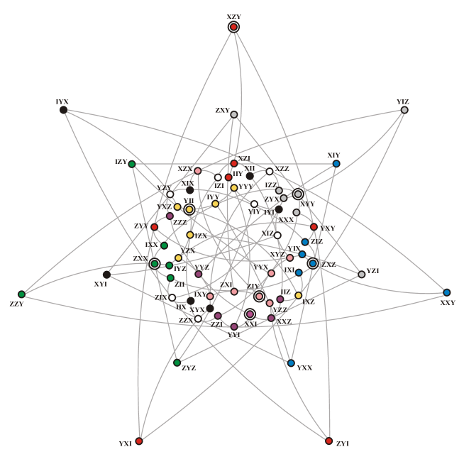
Figure 5: An illustration of a spread of planes of the first kind. The individual planes (as point sets) are distinguished from each other by different colors, the two planes of Heawood type being represented by black and white (empty) bullets; the nuclei/centers of the perp-sets are encircled. This drawing of the split Cayley hexagon of order two, in a form showing its automorphism of order seven, is a slight modification of those given in [schr, psm]. Labeling by the three-qubit observables is taken from [lsv]; see also [sppl, psh].

A spread of the second kind features three perp-planes and six Heawood planes, no two of the latter sharing the same Heawood graph. As any three mutually disjoint planes of $\mathcal{W}(5,\,2)$ belong to two distinct spreads, through our three perp-planes goes another spread of the same kind; its six Heawood planes are nothing but the complements of the former six planes in the corresponding six Heawood graphs. The three nuclei of the perp-planes lie on a line of the ambient space PG$(5,\,2)$ that does not belong to the $\mathcal{W}(5,\,2)$ (i. e. it is not totally isotropic with respect to the select symplectic polarity in the ambient PG$(5,\,2)$). As there are altogether ($651-315=$) 336 such lines (see, for example, [hir]), we have $2\times 336=672$ spreads of this second kind. Here is a particular pair of spreads of this kind on the same triple of perp-planes, the latter being listed first:

$$\{\underline{YZI},ZXY,XYY,YIX,IZX,XXZ,ZYZ\},$$

$$\{\underline{IXI},IXZ,IIZ,ZXZ,ZIZ,ZXI,ZII\},$$

$$\{\underline{YYI},ZZI,XXI,ZZY,XXY,YYY,IIY\},$$

$$\{IYX,XYI,IIX,XYX,XII,XIX,IYI\},$$

$$\{XZY,YIZ,XIY,YZZ,ZZX,ZIX,IZI\},$$

$$\{IZY,YZY,YII,IXX,IYZ,YYZ,YXX\},$$

$$\{XZX,ZZZ,IXY,XYZ,YIY,ZYX,YXI\},$$

$$\{XZI,ZYY,ZXX,YYX,XIZ,YXY,IZZ\},$$

$$\{YXZ,YZX,ZYI,ZIY,XXX,XZZ,IYY\},$$

and

$$\{\underline{YZI},ZXY,XYY,YIX,IZX,XXZ,ZYZ\},$$

$$\{\underline{IXI},IXZ,IIZ,ZXZ,ZIZ,ZXI,ZII\},$$

$$\{\underline{YYI},ZZI,XXI,ZZY,XXY,YYY,IIY\},$$

$$\{YZY,IZI,XZZ,YIY,XIZ,ZZX,ZIX\},$$

$$\{XZX,XZI,ZYX,YXX,ZYI,YXI,IIX\},$$

$$\{XYI,ZXX,YZX,ZZZ,YXZ,IYY,XIY\},$$

$$\{XIX,ZYY,YYZ,XYX,ZIY,IYI,YIZ\},$$

$$\{IZY,IXX,IYZ,XYZ,XXX,XII,XZY\},$$

$$\{IYX,YII,IXY,YZZ,YYX,YXY,IZZ\}.$$

This particular pair of spreads is also illustrated in Figure 6; here the union of any two Heawood planes represented by the same color forms a copy of the Heawood graph.

  

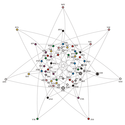
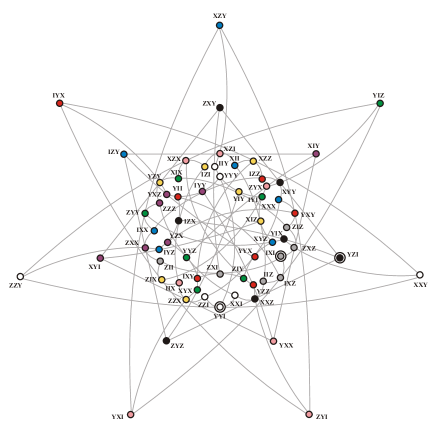
Figure 6: A diagrammatical visualization of the structure of the two spreads of second kind that share three perp-planes, the latter being represented by black, gray and white (empty) bullets; like in the previous figure, the nuclei/centers of the corresponding perp-sets are encircled.

In a skew embedded hexagon, however, neither of the above-described two patterns can be found; this is mainly due to an insufficient number of planar points, but also due to the way how these points are arranged with respect to each other.

3.2 Skew-embedded hexagon, linear doilies and
contextuality

The fact that a copy of the split Cayley hexagon of order two embedded skewly into $\mathcal{W}(5,2)$ features non-planar points has a number of interesting consequences. We will briefly address one of them. Given a skew embedded hexagon, like the one depicted in Figure 7, let us pick up in it a line that consists solely of non-planar points, for example the line $IIZ-XIZ-XII$ (drawn black in Figure 7). Through each point of this line there pass one line that does not belong to the plane of $\mathcal{W}(5,2)$ defined by the other two concurrent lines at this point; these are the lines $IIZ-YZZ-YZI$ (via point $IIZ$ – red), $XIZ-YYY-ZYX$ (via $XIZ$ – yellow) and $XII-XXY-IXY$ (via $XII$ – blue). Clearly, these three lines are pairwise disjoint as otherwise our generalized hexagon would contain triangles, which is impossible as its smallest ordinary polygons are hexagons. These three lines define a unique linear doily, namely the one depicted at the bottom of Figure 7. However, this doily shares with our hexagon two more lines (shown in gray) that are disjoint from each other and also from any of the three lines, i. e. they form with the three lines a spread of lines of the doily. It is obvious that such a set of six lines is the maximum set of lines a doily and a skew-embedded hexagon can share; indeed, assuming that our doily shares an additional line with the hexagon that is skew to the black line (i. e. not incident with it) would mean that the latter would contain quadrangles, which contradicts its definition.

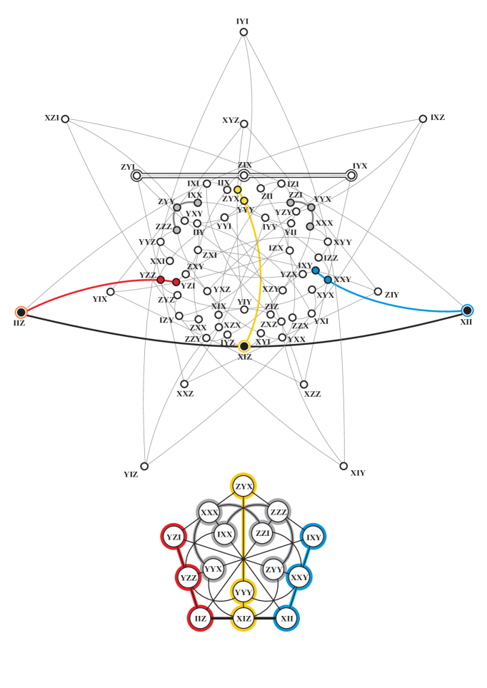
Figure 7: An illustration of the procedure that shows that to each ‘non-planar’ line (black) of a skew embedded split Cayley hexagon of order two (top) one can associate a unique linear doily (bottom) that shares with it the maximum possible number of lines. The horizontal highlighted line of the hexagon is its axis; the meaning of the remaining colored lines is explained in the text.

The above-described relation can also help us understand why a classically embedded hexagon and a doily share just three lines belonging to a grid of the doily. For if we disregard in Figure 7 the three colored lines that occur only in skew embedded hexagons, the remaining three lines (i. e. the black line and the two gray lines) indeed belong to a particular grid of the doily in question!

By a computer search we have found out that there are only three more patterns of lines a linear doily can share with a skew embedded hexagon. One of them is an already mentioned set of three mutually disjoint lines that belong to some grid of the doily. There exists another three-line pattern, namely that comprising two disjoint lines having a common transversal; slightly rephrased, this pattern entails any three lines forming sides of a quadrangle in the doily. The remaining type features two intersecting lines. These can readily be illustrated employing the copy of skew embedded hexagon depicted in Figure 8. To this end, let us consider three particular linear three-qubit doilies, namely the doilies whose all 15 observables feature $I$ on the first qubit (the ‘left’ doily), on the second qubit (the ‘middle’ doily) and on the third qubit (the ‘right’ doily). From Figure 8 one can easily discern that the ‘left’ doily (red) shares with the hexagon the following three lines $IXX-IZZ-IYY$, $IYY-IZX-IXZ$ and $IXZ-IIZ-IXI$, the middle one being indeed incident with either of the remaining two that are disjoint. On the other hand, the ‘right’ doily (blue) has two concurrent lines in common with the hexagon: $XZI-IZI-XII$ and $IZI-YZI-YII$. For the sake of completeness, we also mention that the ‘middle’ doily (not shown) shares with the hexagon the maximal pattern, composed of the five lines $ZIY-IIY-ZII$, $YII-IIX-YIX$, $ZIX-XIY-YIZ$, $XIX-YIY-ZIZ$ and $XIZ-IIZ-XII$ forming a spread, and the line $ZII-IIX-ZIX$.

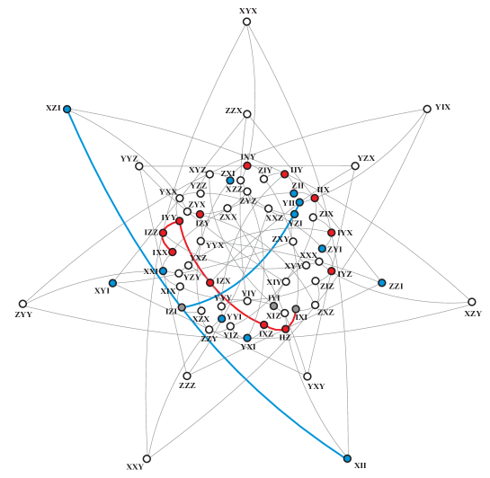
Figure 8: A different copy of skew embedded hexagon (whose axis is the line $YYZ-IXY-YZX$) employed to illustrate additional doily-hexagon intersection patterns. The points and (hexagon-shared) lines of the two doilies are highlighted in different colors, the three points that belong to both the doilies being colored gray.

Apart from classification’s results of their own importance, there is another crucial aspect stemming from the above-discussed intersection properties. Let us consider a doily having with a skew embedded hexagon two concurrent lines in common. It is easy to see that out of the ten grids in this doily, there are four of them that do not contain any of the two shared lines. That is, these four grids are fully contained in the complement of the hexagon. A similar situation also occurs in the above-described three-line pattern; in this case the corresponding doily has just two grids devoid any of the three lines and, so, lying fully in the hexagon’s complement. As grids are the simplest, and so fundamental, quantum contextual structures in multi-qubit symplectic polar spaces, their occurrence in the complements of skew embedded hexagons lends itself as one of the most natural justifications why these complements are contextual.

4 The contextuality of $\mathcal{W}(5,2)$ and the classical embedding of $\mathcal{H}$

Having a better understanding of the difference between the two symplectic embeddings of $\mathcal{H}$ and being endowed with a fresh insight on why the complement of a skew-embedded $\mathcal{H}$ is contextual (by containing three-qubit grids), we can now address our main objective: the relevance of hexagon’s classical embeddings for the issue of three-qubit contextuality.

Recently, the authors of [muller2023new] made the key (computer-based) discovery that the degree of contextuality of the configuration comprising all 315 line-contexts of $\mathcal{W}(5,2)$ is equal to $63$, and not $90$ (= the number of negative lines) as previously proposed by [Cab10]. In addition, and more importantly, they found out that the 63 unsatisfiable contexts of this configuration are in bijection with 63 lines of a copy of $\mathcal{H}$ that is embedded classically into $\mathcal{W}(5,2)$. These facts came as a big surprise to us and prompted us to have a closer look at what is going on here. We will provide first some algebraic-geometrical arguments for the occurrence of the number $63$. Then, employing a line-layered decomposition of the hexagon, we will demonstrate on several examples how the contextuality properties of a three-qubit configuration having three-element contexts can simply be read off from its generic intersection with a classically-embedded copy of $\mathcal{H}$.

4.1 The degree of contextuality of $\mathcal{W}(5,2)$ is sixty-three

In [muller2023new] the proof that the degree of contextuality of $\mathcal{W}(5,2)$ is $63$ was obtained by computer. After translating the problem of finding an NCHV model into the resolution of a linear system over $\mathbb{F}_{2}$, the authors took advantage of a SAT solver to provide an explicit model where all but $63$ of the $315$ constraints imposed by the observable-labelled lines of $\mathcal{W}(5,2)$ are satisfied. This existence of an explicit model proves that the degree of contextuality $d$ of $\mathcal{W}(5,2)$ satisfies $d\leq 63$. In [muller2023new] the inequality $d\geq 63$ was deduced from the fact that the SAT solver was unable to find an explicit NCHV model with at most $62$ constraints, showing $d\geq 63$. It turns out that this second inequality can be obtained from a tiling of the lines of $\mathcal{W}(5,2)$ by doilies. Recall [sbhg21] that $\mathcal{W}(5,2)$ features two kind of doilies, referred to as linear and quadratic. One can define (see Section 2 of [sbhg21]) a quadratic doily as the intersection of a hyperbolic quadric and an elliptic one in $\mathcal{W}(5,2)$. From (4) and (7) for $n=3$ in Section 2 there are $36$ of the former and $28$ of the latter type, which yields $36\times 28=\numprint{1008}$ quadratic doilies in total. The symplectic group, $Sp(6,2)$, acts transitively not only on the lines of $\mathcal{W}(5,2)$, but also on pairs of quadrics. Two quadrics define what is called a Veldkamp line, a geometry built from geometric hyperplanes of $\mathcal{W}(5,2)$ where $Sp(6,2)$ acts [VL10]. The geometry of these specific pairs of quadrics, whose intersection define a quadratic doily, has been investigated in full detail in [levay2017magic]. Each line of $\mathcal{W}(5,2)$ is shared by $48$ different doilies and, by transitivity of $Sp(6,2)$, the $\numprint{1008}$ quadratic doilies cover all the $315$ lines/contexts of $\mathcal{W}(5,2)$. Now recall (see Section 2) that each doily features three constraints that cannot be satisfied. So the restriction to a doily of a NCHV model of $\mathcal{W}(5,2)$ should induce at least $3$ constraints on each doily of $\mathcal{W}(5,2)$. This implies that the degree of contextuality $d$ of $\mathcal{W}(5,2)$ should satisfy the following inequality:

$$d\geq\dfrac{\numprint{1008}\times 3}{48}=63.$$ (14)

Similar group-theoretic arguments can be used if we consider the tiling of lines by other contextual subgeometries of $\mathcal{W}(5,2)$. For instance, the $336$ linear doilies also cover all the $315$ lines of $\mathcal{W}(5,2)$, and as each line of $\mathcal{W}(5,2)$ sits in $16$ linear doilies, we arrive at the same result: $d\geq\dfrac{336\times 3}{16}=63$.

The above-given group-combinatorial explanation of the number 63 can further be substantiated geometrically in the following sense: given a classically-embedded $\mathcal{H}$ one can find a set of 21 doilies whose 63 shared lines (three per doily) partition the set of lines of this $\mathcal{H}$. Next, the fact that a classical $\mathcal{H}$ encodes quantitative information about the contextuality of $\mathcal{W}(5,2)$ as a whole invokes the thought that this encoding should also manifest on any contextual subgeometry of $\mathcal{W}(5,2)$ whose contexts are lines. And this is indeed the case. However, to see it explicitly, we still need to delve a bit more into the geometric structure of the hexagon.

4.2 Layering of the split Cayley hexagon of order two

Let us pick up a skew-embedded copy of the hexagon, e.g. the one shown in Figure 9, and highlight its axis by black color. Given this line, the remaining 62 lines split into three distinct sets. The first set comprises six lines (yellow ones), each being incident with the axis. The second set features 24 lines (gray), each being incident with some yellow one. The last set consists of the remaining 32 lines; these lines can be divided into two disjoint, isomorphic sets of 16 elements each – the two sets being distinguished by blue and red colors.

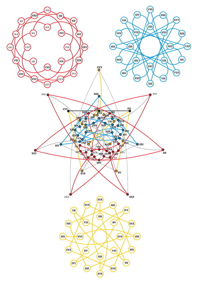
Figure 9: An illustration of the line-distribution within the hexagon.

To see finer traits of the structure of the hexagon, one can redraw the three main ‘layers’ or ‘domains’ of the hexagon, namely red (top left), blue (top right) and yellow (bottom) in the most symmetric way. Note that both the red and blue domains can each be viewed as a pair of circumscribed octagons, either of them being isomorphic to the same $(24_{2},16_{3})$-configuration. In the illustration of the yellow domain each observable is represented by two different (opposite) points and the affine part of each yellow line has four distinct images forming a quadrangle. Our option for such a rendering of the yellow layer is simple: if one stacks all the three figures above each other then the corresponding three observables at a given position define a particular gray line of the hexagon; for example, the three topmost observables form the gray line $XXI-ZYX-YZX$.

4.3 A simple recipe how to get from a skew-embedded hexagon a classically-embedded one, and vice versa

The above-described layered structure of the hexagon turns out to be very relevant to better understand the relation between the two types of embeddings of the split Cayley hexagon of order two. In fact, there exists a rather simple recipe that ‘transforms’ a skew hexagon into a classical one. Let us start with the skew hexagon shown in Figure 9. Keep the three observables of the axis intact. On each yellow line, swap the two remaining observables. On each red (blue) line leave each observable intact and on each blue (red) line replace its observable by that which is the product of a swapped yellow observable and a fixed red (blue) observable on the corresponding gray line. What we get is a copy of a classically embedded hexagon, depicted in Figure 10, that shares 39 lines with the original skew hexagon: the black line, the 6 yellow lines, the 16 blue lines and the 16 red lines.

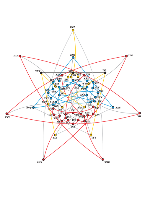
Figure 10: The classical hexagon we get from the skew-embedded one by applying the procedure described in the text.

This construction only works if the black (reference) line is the axis of the skew hexagon. Obviously, we can reverse the process and start with a classically-embedded hexagon to get a skew one. In this case any of its 63 lines can be taken as the reference black line, so we get 63 different skew copies from a given classical one. As there are 120 different classical copies of the hexagon in $\mathcal{W}(5,2)$, the above property also implies that there are as many as $120\times 63=7560$ skew embedded hexagons living in $\mathcal{W}(5,2)$ – confirming the result of [holweck2022three] based on an exhaustive computer search.

4.4 Classically-embedded hexagons encode three-qubit
contextuality

As already stressed, the fact that any set of 63 unsatisfiable constraints associated with all the 315 lines/contexts of the three-qubit symplectic polar space forms a $63_{3}$-configuration isomorphic to a copy of the split Cayley hexagon of order two embedded classically into the space in question seems to be just part of a bigger story, as something similar is taking place for the lines located on both elliptic and hyperbolic quadrics, as well as on doilies of $\mathcal{W}(5,2).$

Let start with elliptic quadrics. By a computer search we have found that each elliptic quadric features 9 pairwise disjoint unsatisfiable lines/contexts forming a spread. On the other hand, each classically embedded hexagon shares with each elliptic quadric such a set of 9 lines. An example is illustrated in Figure 11.

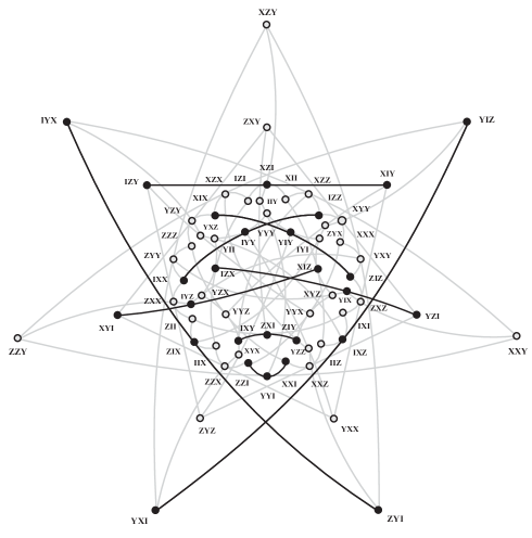
Figure 11: The generic intersection of a classical hexagon with an elliptic quadric: nine mutually disjoint lines that are at maximum distance from each other, aka a distance-three spread of the hexagon. Note that these nine lines cover all the 27 points of the quadric.

Next, each classically embedded hexagon shares with each hyperbolic quadric exactly 21 lines, forming a pattern isomorphic to the one shown in Figure 12. People familiar with graph theory may readily recognize this pattern as the Heawood graph, also known as the point-line incidence graph of the Fano plane, whose vertices are represented by bigger bullets, each of its edges being supplied with one more point/observable to represent a full line of the three-qubit $\mathcal{W}(5,2)$. Using a computer we have verified that each three-qubit hyperbolic quadric features 21 unsatisfiable lines whose arrangement is isomorphic to that depicted in Figure 12.

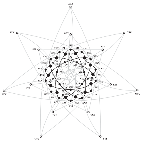
Figure 12: The generic intersection of a classical hexagon with a hyperbolic quadric: 21 lines forming edges of the Heawood graph. As in the previous case, the 21 lines comprise all the 35 points of the quadric.

A similar analysis carried out for doilies living in $\mathcal{W}(5,2)$ showed the same result. The three unsatisfiable constraints a doily features, forming always a spread in one of the doily’s grids, are those three lines that the doily shares with a particular copy of a classical hexagon.

The message from the above-given observations is more than obvious: the degree of contextuality of a contextual quantum geometry of the three-qubit $\mathcal{W}(5,2)$ whose contexts are i) all the 315 lines of the space, ii) all the lines of an elliptic quadric, iii) all the lines of a hyperbolic quadric or iv) all the lines of a doily is equal to the number of lines each of these geometries shares with a classically embedded hexagon, with the understanding that each shared line corresponds to an unsatisfiable context. A natural generalization of these findings is that this should hold for any contextual sub-geometry of $\mathcal{W}(5,2)$ whose contexts are lines. In other words, classically-embedded copies of $\mathcal{H}$, although being non-contextual by themselves, are found to rule three-qubit contextuality by being a reliable tool not only to check whether a particular subgeometry of $\mathcal{W}(5,2)$ is contextual, but also, and still mysteriously, to ‘extract’ from this subgeometry exactly that part that makes it non-contextual!

As a particular stance of this conjecture, let us consider the complement of a skew-embedded hexagon, which is a contextual $(63_{12},252_{3})$-configuration [holweck2022three]. Analyzing complements of several different copies of skew-embedded hexagons we always arrived at the same result: each complement featured 24 unsatisfiable constraints that were exactly those 24 lines in which the given skew-embedded hexagon differs from the classical one derived from it using the procedure described in Section 4.3; thus, for example, if we consider the complement of the skew hexagon shown in Figure 9 then its 24 unsatisfiable lines are exactly the 24 gray lines of its derived classical sibling portrayed in Figure 10!

5 Some experimental verification using the
IBM Quantum Experience

The advent of accessible NISQ computers has allowed researchers to test whether contextual geometries exhibit the predicted quantum behaviour in reality, see for example [laghaout2022demonstration, holweck2021testing, Kelleher_2_qubit_games]. Given the accelerated development of such technologies, and their widening availability for research purposes, it is easier than ever to experimentally test out the predictions of NCHV models mentioned in the introduction. First, one needs a quantitative test on our geometry that can rule out NCVM models in favour of those predicted by quantum mechanics (QM). In this section we examine such a test.

5.1 Cabello inequality

In 2010 Cabello [Cab10] introduced an inequality dependent upon the number of satisfiable constraints in a contextual geometry. The quantity $\chi$ is defined as the sum of expectation values of all constraints, with negative ones picking up a sign change,

$$\chi \equiv\sum_{i}\langle C_{i}\rangle-\sum_{j}\langle C^{\prime}_{j}\rangle$$ (15)

$$\chi \leq\begin{cases}N,\quad\qquad\,\text{QM}\\ N-2d,\quad\text{HV}\end{cases}$$ (16)

where the $C_{i}$ are the positive contexts in the geometry, $C^{\prime}_{j}$ the negative ones, $\langle\cdot\rangle$ their expectation values, $N$ the total number of contexts, and $d$ the degree of contextuality. In the QM regime, all constraints are satisfied with expectation value $+1$ for positive contexts and $-1$ for negative ones, and so $\chi$ provides the number of constraints in total. For NCHV models, some constraints will not be satisfied and induce an additive factor of $-2$ into this expression.

The inequalities provide an upper bound on the measured value of $\chi$ based on whether all constraints are satisfiable (QM) or there is a NCHV model constraining some measurement outcomes (HV).

5.2 Measuring contextuality on a NISQ computer

One can experimentally test the contextuality (that is, the value of $\chi$ in (16)) of a given labelled geometry via the IBM Quantum Experience [ibmq]. The methodology is straightforward: for a given context in a geometry labelled by $3$-qubit operators, measure the values of the operators at each point of the context and combine to get the measured parity of the line. Repeat for all lines in the geometry, and sum together weighted by their signed parities. If the final result is greater than the upper bound $N-2d$ given in (16), then we have demonstrated the contextuality of the geometry.

There is but one issue to address first before implementing this in a circuit. For a context containing three operators $\mathcal{O}_{1},\mathcal{O}_{2},\mathcal{O}_{3}$, when measuring the state of operator $\mathcal{O}_{1}$ one has destroyed the quantum state, and measurements of $\mathcal{O}_{2},\mathcal{O}_{3}$ will no longer be descriptive of the context as a whole. To circumvent this, we introduce additional “delegation” qubits into the circuit. The purpose of these qubits is to record the “state” of the context under each operator, without destroying it via measurements on the original register.

Firstly, we initialise three qubits labelled $q_{1},q_{2},q_{3}$ encoding the state of the three qubits the context will act on. Depending on the operator $\mathcal{O}_{1}$ of the context, gates are applied to these qubits to change their basis from the computational one to the “operational” $\mathcal{O}_{1}$-basis (see Figure 13). Then CNOT gates are applied between the qubits $q_{1},q_{2},q_{3}$ and a delegation qubit $d_{1}$ to record the state onto that new qubit (see Figure 14). The inverse gates are applied to the $q_{i}$ to revert them back to the original state. Finally, this process is repeated for operators $\mathcal{O}_{i}$ and delegation qubits $d_{i}$ for $i=2,3$. The states of the delegation qubits are then measured to record the measurement outcomes of the operators $\mathcal{O}_{1},\mathcal{O}_{2},\mathcal{O}_{3}$.

Operator	Gates
$I$	$\cdot$
$X$
$Y$
$Z$

Figure 13: Basis change gates to convert from the computational basis to the “operational” one, for a given context operator. For the identity $I$, no basis change gates nor CNOT gates are applied.

Figure 14: Quantum circuit demonstrating triple measurement on a context via delegations. Qubits $q_{1},q_{2},q_{3}$ encode the three-qubit state of the context. State is passed down to delegation qubits $d_{1},d_{2},d_{3}$ sequentially via CNOT gates. Basis change gates are suppressed.

For example, in measuring $\mathcal{O}_{1}=XIY$, the gate $H$ is applied to $q_{1}$, no gate to $q_{2}$, and $S^{{\dagger}}H$ to $q_{3}$. Then CNOTs are applied between $q_{1}$ and $d_{1}$, and $q_{3}$ and $d_{1}$, with $d_{1}$ acting as the target in each case. Inverse gates $H$, $HS$ are then applied to $q_{1},q_{3}$ respectively, before measurement taken on $d_{1}$.

We have implemented the above circuitry for two contextual geometries: the elliptic quadric $\mathcal{Q}^{-}(5,2)$ and the complement $\overline{\mathcal{H}_{S}}$ of the skew-embedded hexagon. The measured contextuality $\chi$ for each is given in Table 1, compared with the QM and HV upper bounds. In each case, individual contexts were measured over $\numprint{8192}$ shots on the “Lagos” IBM NISQ backend and also on a noiseless simulated quantum backend. When run on the simulated backend, the results give $\chi_{sim}=N$ as expected from (16), however the inherent noise in the “Lagos” backend reduces the measured value of $\chi_{NISQ}$ to somewhere still above the HV bound.

Geometry	$d$	$N$	$N-2d$	$\chi_{sim}$	$\chi_{NISQ}$
$\mathcal{Q}^{-}(5,2)$	9	45	27	45	27.86328
$\overline{\mathcal{H}_{S}}$	24	252	204	252	212.53735

Table 1: Results for experimental tests of Cabello contextuality measure $\chi$ run on both a noiseless simulator and the IBM “Lagos” backend. In both geometries $\mathcal{Q}^{-}(5,2)$ and $\overline{\mathcal{H}_{S}}$, the measured contextuality $\chi_{NISQ}$ is greater than the upper bound predicted by a non-contextual hidden variable model HV.

Note that in both cases our experiments reveal the contextual nature of the configuration. Our procedure to test Cabello’s inequalities follow and slightly improves the experiments of [laghaout2022demonstration, holweck2021testing]. In particular, this time we delegated the measurements corresponding to the three observables of a context to three different delegation qubits (instead of a single qubit used in the previous cited work). Although this new procedure reduces the gap between the experimental value and the classical bound, it has the advantage of collecting the result for each of the three observables independently.

6 Conclusion

This paper provides substantial insights into the role played by the smallest split Cayley hexagon $\mathcal{H}$ in its classical embeddings into $\mathcal{W}(5,2)$ in observable-based three-qubit contextuality, as first elaborated by three of us in [holweck2022three]. We have demonstrated that classically-embedded copies of $\mathcal{H}$ fully encode the basic information about distinguished contextual configurations living in $\mathcal{W}(5,2)$, namely doilies, both types of quadrics, complements of skew-embedded $\mathcal{H}$’s as well as the configuration formed by all the 315 lines of the space. Given such a configuration, one can always find some classically-embedded copy of $\mathcal{H}$ that shares with this configuration exactly those contexts that are unsatisfiable by an NCHV model! It is truly amazing to realize that the three-qubit $\mathcal{W}(5,2)$ is endowed with the distinguished subgeometry, $\mathcal{H}$, that – although being itself non-contextual – is able to single out from a large variety of contextual configurations exactly those parts that ‘responsible’ for their contextual behavior.

Interestingly, we have already at hand some hints that something similar is taking place in the next case in the hierarchy – the four-qubit $\mathcal{W}(7,2)$. By making use of the Lagrangian Grassmannian mapping of type $LGr(3,6)$ that sends planes of $\mathcal{W}(5,2)$ into points of a hyperbolic quadric $\mathcal{Q}^{+}(7,2)$ of $\mathcal{W}(7,2)$ we already found on this quadric a particular configuration that can be regarded as a four-qubit analog of a three-qubit Heawood-graph-underpinned configuration described in Section 4.4 (cf. Figure 12). This particular configuration contains 135 points and 315 lines, with seven lines through a point and three points on a line, and – being isomorphic to the dual polar space $\mathcal{DW}(5,2)$ – has the desired property that it shares with each of the 120 $\mathcal{W}(5,2)$’s located on the $\mathcal{Q}^{+}(7,2)$ a copy of $\mathcal{H}$, the latter being indeed embedded classically into the corresponding $\mathcal{W}(5,2)$; moreover, it also contains 36 (one per each hyperbolic quadric of $\mathcal{W}(5,2)$ as dictated by $LGr(3,6)$-correspondence) copies of the point-plane incidence graph of PG$(3,2)$. What remains to be checked is whether there exists a four-qubit analog of a ‘classical’ $\mathcal{H}$ of $\mathcal{W}(5,2)$, that is a configuration that picks up from each $\mathcal{Q}^{+}(7,2)$ of $\mathcal{W}(7,2)$ a configuration isomorphic to our $(135_{7},315_{3})$-one. An affirmative answer to this computationally rather challenging task would mean, among other things, that the degree of contextuality of a four-qubit hyperbolic quadric is 315 and that of the whole $\mathcal{W}(7,2)$ amounts to 1 575.