Stability of Ecological Systems: A Theoretical Review

Abstract

The stability of ecological systems is a fundamental concept in ecology, which offers profound insights into species coexistence, biodiversity, and community persistence. In this article, we provide a systematic and comprehensive review on the theoretical frameworks for analyzing the stability of ecological systems. Notably, we survey various stability notions, including linear stability, sign stability, diagonal stability, D-stability, total stability, sector stability, structural stability, and higher-order stability. For each of these stability notions, we examine necessary or sufficient conditions for achieving such stability and demonstrate the intricate interplay of these conditions on the network structures of ecological systems. Finally, we explore the future prospects of these stability notions.

organization=School of Data Science and Society and Department of Mathematics, University of North Carolina at Chapel Hill,city=Chapel Hill, postcode=27599, state=NC, country=USA

organization=Channing Division of Network Medicine, Department of Medicine, Brigham and Women’s Hospital, Harvard Medical School,city=Boston, postcode=02115, state=MA, country=USA

organization=Carl R. Woese Institute for Genomic Biology, Center for Artificial Intelligence and Modeling, University of Illinois at Urbana-Champaign,city=Champaign, postcode=61801, state=IL, country=USA

1 Introduction

Ecological systems are usually subject to continual disturbances or perturbations, and their responses are often characterized quantitatively as stability, a fundamental concept rooted in dynamical systems and control theory [56, 138, 156, 177, 187, 227, 228, 233, 256]. Loosely speaking, an ecological system is stable if its state represented by a vector of its species abundances, do not change too much under small perturbations. Therefore, understanding the stability of ecological systems is particularly important due to its implications for species coexistence, biodiversity, and community persistence [74, 108, 115, 121, 125, 154, 186, 255]. More importantly, these implications can contribute to the development of effective interventions and policies that maintain the overall health of ecological systems [81, 95, 105, 131].

Numerous mathematicians, physicists, and ecologists have explored the stability of ecological systems. In his pioneer work, May linearized an unspecified nonlinear dynamical system around an equilibrium to perform the local linear stability analysis of ecological systems [165, 167, 168]. The local linear stability is completely characterized by the eigenvalues of the Jacobian matrix (of the unspecified dynamical model), which is often called the community matrix in the ecological contexts. If all the eigenvalues of the community matrix have negative real parts, the ecological system is locally stable around the equilibrium. By incorporating random matrix theory, May successfully derived a simple condition to characterize the stability of ecological systems. While there have been intense debates about the relationship between stability and complexity over the past five decades [170, 183, 201, 213, 232, 258, 262, 277], May’s result offers a powerful foundation for analyzing the stability of ecological systems with diverse structural characteristics, such as interaction types [9], degree heterogeneity [272], self-regulation [30], modularity [114], and more.

May’s framework does not need to know the dynamical model of the ecological system. Instead, it focuses on the Jacobian matrix of the unspecified dynamical model. Hence, the framework is model-implicit. In the past, actually many ecological models, such as the generalized Lotka-Volterra (GLV) model (1910) [49, 162], Holling type II model (1959) [2, 237], and MacArthur’s consumer-resource model (1970) [1, 70], have been proposed to study the dynamics of ecological systems. Remarkably, the GLV model is the most commonly used model in the stability analysis of ecological systems due to its simplicity [5, 13, 42, 43, 57, 107, 144, 279]. Most of these findings rely on Lyapunov theory, which allows us to determine the stability of a system without explicitly integrating the differential equation. Lyapunov theory encompasses two fundamental methods. One is based on linearization (e.g., May’s approach), which is often referred to as the Lyapunov indirect method, while the other is called the Lyapunov direct method. The essence of Lyapunov direct method is to construct the so-called Lyapunov function, an “energy-like” scalar function whose time variation can be viewed as the “energy dissipation.” It is not restricted to small perturbations, and in principle can be applied to all dynamical systems. However, we lack a general theory to find a suitable Lyapunov function for an arbitrary dynamical system. Instead, we have to rely on our experience and intuition. Notably, certain diagonal-type Lyapunov functions are useful for the stability analysis of ecological systems described by the GLV model [137].

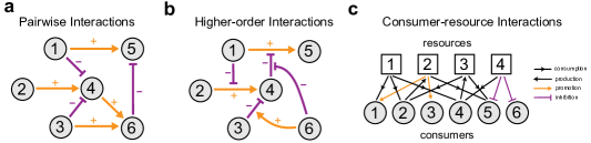
Figure 1: Pairwise interactions versus higher-order interactions in ecological systems. (a) Pairwise interspecies interactions. (b) Higher-order interspecies interactions. (c) Consumer-resource interactions naturally implies higher-order interspecies interactions.

The feasibility of an ecological system, which concerns whether a specific set of conditions or parameters can support the system over time, can also impact its stability [7, 18, 109, 112, 189, 246]. Intriguingly, the relationship between feasibility and stability is noteworthy when dealing with ecological systems described by the GLV model or MacArthur’s consumer-resource model. It has been proved that under certain conditions, the feasibility of such systems can imply their stability [59, 246]. Moreover, feasibility is closely related to a concept known as structural stability, which reflects the ability of an ecological system to qualitatively maintain its dynamics and overall behavior under small disturbances or perturbations of the system model itself [215]. A great amount of metrics have been proposed to quantify the structural stability of ecological systems through feasibility analysis [112, 215, 222].

Recently, there has been a growing interest in higher-order interactions within ecological systems, which refers to the intricate relationships that extend beyond pairwise interspecies interactions [27, 32, 101, 113, 155], see Figure 1a, b. Mathematically, these higher-order interactions emerged in an ecological system can be naturally represented as a hypergraph, where its hyperedges can connect an arbitrary number of nodes [44]. The resulting dynamics can be expressed in the form of polynomials [67]. The analysis of hypergraph dynamics often involves the application of tensor theory [65, 67, 199, 249], which deals with multidimensional arrays generalized from vectors and matrices [62, 66, 68]. Lyapunov theory can also be leveraged to analyze the stability of polynomial dynamical systems [3]. Furthermore, the consumer-resource model can be implicitly considered as an instance of higher-order interactions, with consumer species as nodes and resources as hyperedges, see Figure 1c. Increasing evidence has revealed that higher-order interactions play a significant role in the stability of ecological systems [27, 101, 113].

Table 1: Summary of stability notions that have been used to study ecological systems.

Notion	Main Model	Characteristics	Key References
Linear Stability	Linear model (3), GLV model (10)	Characterizing the eigenvalue spectrum of the community matrix M through random matrix theory.	[9, 10, 30, 36, 38, 96, 100, 111, 114, 128, 148, 165, 167, 200, 205, 231, 246, 251, 271, 272, 273]
Sign Stability	Linear model (3)	Assessing stability based solely on the signs of the elements in the community matrix M without considering their magnitudes.	[11, 77, 120, 132, 161, 169, 208, 270]
Diagonal Stability	GLV model (10)	The diagonal stability of the interaction matrix A, i.e., there exists a diagonal matrix P such that $\textbf{A}^{\top}\textbf{P}+\textbf{P}\textbf{A}\prec 0$, implies the Lyapunov stability of the GLV model.	[19, 20, 21, 22, 42, 43, 100, 107, 112, 122, 126, 137, 144, 173, 212, 235, 264, 268]
D-Stability	GLV model (10)	The D-stability of the interaction matrix A, i.e., the matrix XA is stable for any positive diagonal matrix X, implies that any feasible equilibrium of the GLV model is locally stable.	[24, 72, 90, 100, 134, 215]
Total Stability	GLV model (10)	The total stability of the interaction matrix A, i.e., any principal sub-matrix of A is D-stable, implies that a new feasible equilibrium of the GLV model remains locally stable after the removal or extinction of certain species.	[158, 159, 160, 208]
Sector Stability	Generic population dynamics model (26)	A semi-feasible equilibrium point is called sector stable if every solution that starts within a non-negative neighborhood remains in the same or an even larger non-negative neighborhood and eventually converges to that equilibrium point.	[59, 106]
Structural Stability	GLV model (10)	Measuring the capacity to qualitatively maintains the dynamics under small disturbances or perturbations through feasibility analysis of the GLV model.	[17, 112, 193, 198, 211, 215, 220, 222, 239, 240, 244]
Higher-order Stability	GLV model with higher-order interactions (32), MacArthur’s consumer-resource mode (38)	Analyzing the stability of ecological systems with (implicit) higher-order interactions via polynomial systems theory and local stability analysis.	[3, 4, 6, 18, 27, 51, 58, 59, 62, 78, 80, 84, 87, 98, 101, 113, 139, 229, 236, 250, 278]

Most significantly, the stability of an ecological system is profoundly determined and characterized by its underlying network structure, which captures how species influence one another and how disturbances or perturbations propagate among species. In this article, we provide a systematic and inclusive literature review on the theoretical frameworks for analyzing the stability of ecological systems. In Section 2, we briefly review the fundamentals of Lyapunov theory, which acts as a foundation for the stability analysis of ecological systems. From Section 3 to 10, we comprehensively survey various stability notions, including linear stability, sign stability, diagonal stability, D-stability, total stability, sector stability, structural stability, and higher-order stability, see Table 1. For each of these stability notions, we examine necessary or sufficient conditions that are required to establish such stability and illustrate the complicated relationships between these conditions and the network structures of ecological systems. Finally, we discuss the future prospects of these stability notions in Section 11 and conclude in Section 12.

2 Preliminaries

In this section, we review the fundamentals of Lyapunov theory, which plays a significant role in the various stability analyses of ecological systems. We adapt most of the notations and results from the comprehensive work of [140, 141, 174, 226, 238].

2.1 Definitions of Lyapunov stability

Consider a general $S$-dimensional nonlinear system

$$\dot{\bf x}(t)={\bf f}({\bf x}(t),t)\quad\text{with}\quad{\bf x}(t_{0})={\bf x}_{0},\quad{\bf x}(t)\in\mathbb{R}^{S}.$$ (1)

In most cases, we are interested in the stability of the system near an equilibrium point ${\bf x}^{*}\in\mathbb{R}^{S}$ that satisfies ${\bf f}({\bf x}^{*},t)={\bf 0}$. Without loss of generality, we can shift the origin of the system and assume that the equilibrium point of interest occurs at ${\bf x}^{*}={\bf 0}$. Let M be the Jacobian matrix evaluated at $\textbf{x}^{*}$. Denote $n_{-}$, $n_{0}$, and $n_{+}$ be the numbers of eigenvalues (counting multiplicities) of M with negative, zero, and positive real part, respectively. An equilibrium point is called hyperbolic if $n_{0}=0$, i.e., there are no eigenvalues on the imaginary axis. A hyperbolic equilibrium point is called a hyperbolic saddle if $n_{-}n_{+}\neq 0$. Since a generic matrix has $n_{0}=0$, equilibrium points in a generic dynamical system are typically hyperbolic.

An equilibrium point ${\bf x}^{*}={\bf 0}$ is stable (in the sense of Lyapunov) at $t=t_{0}$ if $\forall\epsilon>0$, $\exists\,\delta(\epsilon,t_{0})>0$ such that

$$||{\bf x}(t_{0})||\leq\delta(\epsilon,t_{0})\Rightarrow||{\bf x}(t)||\leq\epsilon,\text{ }\forall t\geq t_{0}>0.$$

Otherwise, ${\bf x}^{*}$ is unstable, see Figure 2. An equilibrium point ${\bf x}^{*}={\bf 0}$ is asymptotically stable at $t=t_{0}$ if it is stable and locally attractive, i.e., $\exists\,\delta(t_{0})>0$ such that

$$||{\bf x}(t_{0})||\leq\delta(t_{0})\Rightarrow\lim_{t\to\infty}{\bf x}(t)={\bf 0}.$$

An equilibrium point which is stable but not asymptotically stable is called marginally stable, see Figure 2. Both stability and asymptotic stability are defined at a time instant $t_{0}$. In practice, it is often desirable for a system to have a certain uniformity in its behavior. Uniform (asymptotic) stability requires that the equilibrium point is (asymptotically) stable for all $t_{0}>0$. Note that notions of uniformity are only relevant for time-varying or non-autonomous systems. For autonomous or time-invariant systems, (asymptotic) stability naturally implies uniform (asymptotic) stability. The definition of asymptotic stability does not quantify the rate of convergence. The notion of exponential stability guarantees a minimal rate of convergence. An equilibrium point ${\bf x}^{*}={\bf 0}$ is exponentially stable if $\exists\,\delta,\alpha,\lambda>0$ such that

$$||{\bf x}(t_{0})||\leq\delta\Rightarrow||{\bf x}(t)||\leq\alpha||{\bf x}(t_{0})||e^{-\lambda(t-t_{0})},\text{ }\forall t\geq t_{0}.$$

Exponential stability is a very strong form of stability because it implies uniform asymptotic stability.

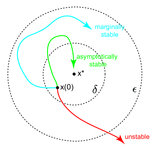
Figure 2: Geometrical implication of stability. For nonlinear systems $\dot{\textbf{x}}(t)=\textbf{f}(\textbf{x}(t),t)$, due to the complex and rich behavior of nonlinear dynamics, various types of stability, e.g., stability, asymptotic stability, and global asymptotic stability, can be discussed. Intuitively and roughly speaking, if all solutions of the system that start out near an equilibrium point ${\bf x}^{*}$ stay near ${\bf x}^{*}$ forever, then ${\bf x}^{*}$ is stable (in the sense of Lyapunov). More strongly, if ${\bf x}^{*}$ is stable and all solutions that start out near ${\bf x}^{*}$ converge to ${\bf x}^{*}$ as $t\to\infty$, then ${\bf x}^{*}$ is asymptotically stable. ${\bf x}^{*}$ is marginally stable if it is stable but not asymptotically stable. This figure was redrawn from [238].

The above definitions of stability, asymptotic stability, and exponential stability are local and only describe the behavior of a system near an equilibrium point. We call an equilibrium point globally (asymptotically or exponentially) stable, if it is (asymptotically or exponentially) stable for all initial conditions ${\bf x}_{0}\in\mathbb{R}^{S}$. Though global stability is very desirable, it is very difficult to achieve in many systems. Note that linear time-invariant (LTI) systems are either asymptotically stable, or marginally stable, or unstable. Moreover, linear asymptotic stability is always global and exponential, and linear instability always implies exponential blow-up. The above refined notions of stability are explicitly needed only for nonlinear systems.

2.2 Lyapunov’s indirect method

Lyapunov’s indirect method is based on linearization, and is concerned with the local stability of a nonlinear system and is based on the intuition that a nonlinear system should behave similarly to its linearized approximation for small disturbances or perturbations. The linearization can be used to give a conservative bound on the domain of attraction of the equilibrium point for the original nonlinear system.

For a general nonlinear system (1) with continuously differentiable ${\bf f}({\bf x}(t),t)$ around the equilibrium point ${\bf x}^{*}={\bf 0}$, the system dynamics can be rewritten as

$$\dot{\bf x}(t)={\bf M}(t){\bf x}(t)+{\bf f}_{\text{h.o.t}}({\bf x}(t),t),$$

where ${\bf M}(t)=\frac{\partial{\bf f}({\bf x},t)}{\partial{\bf x}}|_{{\bf x}={\bf x}^{*}}$ is the Jacobian matrix of ${\bf f}({\bf x},t)$ with respect to ${\bf x}$, evaluated at the equilibrium point ${\bf x}^{*}$, and ${\bf f}_{\text{h.o.t}}({\bf x},t)$ represents the higher-order terms in ${\bf x}$. We typically require ${\bf f}_{\text{h.o.t}}({\bf x},t)$ approaches zero uniformly, which is obviously true for an autonomous system. Then $\dot{\bf x}(t)={\bf M}(t){\bf x}(t)$ is called the uniform linearization of the original nonlinear system (1) at the equilibrium point ${\bf x}^{*}={\bf 0}$. If this uniform linearization exists and the Jacobian matrix ${\bf M}(t)$ is bounded, then the uniform asymptotic stability of the equilibrium point ${\bf x}^{*}={\bf 0}$ for the linearization implies its uniform local asymptotic stability for the original nonlinear system.

For an autonomous system $\dot{\bf x}(t)={\bf f}(\textbf{x}(t))$, the linearization is simply an LTI system $\dot{\bf x}(t)={\bf M}{\bf x}(t)$. Denote the eigenvalues of ${\bf M}$ as $\lambda({\bf M})$. We have the following results: (i) if the linearization is strictly stable (i.e., all the eigenvalues of M lie in the closed left half of the complex plane), then the equilibrium point ${\bf x}^{*}={\bf 0}$ is asymptotically stable for the original nonlinear system (note that a real square matrix M that satisfies $\text{Re}[\lambda({\bf M})]<0$ is often called Hurwitz stable); (ii) if the linearization is unstable (i.e., at least one eigenvalue of ${\bf M}$ has positive real part), then the equilibrium point is unstable for the original nonlinear system; (iii) if the linearization is marginally stable (i.e, all eigenvalues of ${\bf M}$ are in the left-half complex plane, but at least one of them is on the imaginary axis), then one can not conclude anything from the linearization—the equilibrium point may be stable, asymptotically stable, or unstable for the original nonlinear system.

2.3 Lyapunov’s direct method

Lyapunov’s direct method (also called the second method of Lyapunov) can be considered as a mathematical extension of a fundamental physical observation. If the total energy of a mechanical or electrical system is continuously dissipated, then the system must eventually settle down to an equilibrium point, no matter whether it is linear or nonlinear. Thus, we may conclude the stability of a system by studying the energy change rate of the system, without explicitly solving the original differential equation (1).

Let ${\bf B}_{\epsilon}$ be a ball of size $\epsilon$ around the origin ${\bf x}={\bf 0}$, i.e., ${\bf B}_{\epsilon}=\{{\bf x}\in\mathbb{R}^{S}:||{\bf x}||<\epsilon\}$. A scalar continuous function $V({\bf x}):\mathbb{R}^{S}\to\mathbb{R}$ is locally positive definite (LPD) if $V({\bf 0})=0$ and ${\bf x}\neq{\bf 0}\Rightarrow V({\bf x})>0$ in the ball ${\bf B}_{\epsilon}$. If $V({\bf 0})=0$ and the above property holds for the whole state space, then $V({\bf x})$ is globally positive definite (GPD). Similarly, a scalar continuous function $V({\bf x})$ is locally (or globally) positive semi-definite if $V({\bf 0})=0$ and ${\bf x}\neq{\bf 0}\Rightarrow V({\bf x})\geq 0$ in the ball ${\bf B}_{\epsilon}$ (or for the whole state space). A scalar continuous function $V({\bf x},t):\mathbb{R}^{S}\times\mathbb{R}_{>0}\to\mathbb{R}$ is locally positive definite if $V({\bf 0},t)=0$ and there exists a time-invariant LPD function $V_{0}({\bf x})$ that is dominated by $V({\bf x},t)$, i.e., $V({\bf x},t)\geq V_{0}({\bf x}),\text{ }\forall t\geq t_{0}$. If $V({\bf 0},t)=0$ and the above property holds for the whole state space, then $V({\bf x},t)$ is globally positive definite. A scalar continuous function $V({\bf x},t)$ is called decrescent if $V({\bf 0},t)=0$ and there exists a time-invariant LPD function $V_{1}({\bf x})$ that dominates $V({\bf x},t)$, i.e., $V({\bf x},t)\leq V_{1}({\bf x}),\text{ }\forall t\geq t_{0}$. A scalar continuous function $V({\bf x},t)$ is called radially unbounded if $\lim_{||x||\to\infty}V({\bf x},t)\to\infty$ uniformly on $t$.

Let $V({\bf x},t)$ be a non-negative function with derivative $\dot{V}({\bf x},t)$ along the trajectories of the system, i.e.,

$$\dot{V}({\bf x},t)=\frac{\partial V}{\partial t}+\frac{\partial V}{\partial{\bf x}}{\bf f}({\bf x},t).$$

Lyapunov’s theorems of equilibrium point stability are summarized in Table 2. Note that they are all sufficiency theorems. If for a particular choice of Lyapunov function candidate $V$, the condition on $\dot{V}$ is not met, we cannot draw any conclusions on the system’s stability. Many Lyapunov functions may exist for the same system. Specific choices of Lyapunov functions may yield more precise results than others.

Table 2: Summary of Lyapunov stability theorems on equilibrium point ${\bf x}^{*}={\bf 0}$ [174].

$V({\bf x},t)$	$-\dot{V}({\bf x},t)$	Stability (in the sense of Lyapunov)
LPD	LPSD	stable
LPD, decrescent	LPSD	uniformly stable
LPD, decrescent	LPD	uniformly asymptotically stable
GPD, decrescent, radially unbounded	GPD	globally uniformly asymptotically stable

For an LTI system $\dot{\bf x}(t)={\bf M}{\bf x}(t)$, we often use a quadratic Lyapunov function candidate $V=\textbf{x}^{\top}\textbf{P}\textbf{x}$, where P is a symmetric positive definite matrix (i.e., $\textbf{x}^{\top}\textbf{P}\textbf{x}>0,\text{ }\forall\textbf{x}\neq{\bf 0}$), denoted as $\textbf{P}\succ 0$. It is easy to derive that

$$\dot{V}=\dot{\textbf{x}}^{\top}\textbf{P}\textbf{x}+\textbf{x}^{\top}\textbf{P}\dot{\textbf{x}}=-\textbf{x}^{\top}\textbf{Q}\textbf{x},$$

where

$${\bf Q}={\bf Q}^{\top}=-(\textbf{M}^{\top}\textbf{P}+\textbf{P}\textbf{M}).$$ (2)

The above equation is often called the Lyapunov equation of the LTI system. If Q is positive definite, then the system is globally asymptotically stable. However, if Q is not positive definite, then no stability conclusion can be drawn. Fortunately, Lyapunov proved a necessary and sufficient condition for an LTI system to be strictly stable. For any symmetric positive definite matrix Q, the unique matrix solution P of the Lyapunov equation (2) is symmetric positive definite. Therefore, we can start by choosing a simple positive definite matrix Q (e.g., the identity matrix I), then solve for P from the Lyapunov equation, and finally verify whether P is positive definite.

3 Linear stability analysis

As a simple application of Lyapunov’s indirect method, linear stability analysis has been extensively applied to ecological systems, helping us better understand the intricate relationships between stability and biodiversity [9, 12, 33, 124, 152, 165, 167, 182, 265]. More significantly, under some special conditions, local stability determined by linear stability analysis implies global stability for certain ecological systems [127].

In his pioneer work, May considered an ecological system of $S$ species coexisting at a feasible equilibrium point ${\bf x}^{*}$ of a dynamical system $\dot{\bf x}(t)={\bf f}({\bf x}(t))$ that describes the time-dependent abundance vector ${\bf x}(t)$ of the $S$ species [165, 167]. Suppose that one species is subjected to a small but sudden population increase or decrease. As a result, other species populations may show immediate changes away from the equilibrium. The manipulated species itself, if with initially increased (or reduced) abundance, may begin to decline (or increase) toward the equilibrium because of self-regulation. These immediate, direct changes can be referred to as first-order effects and described by the linearized equation of the original dynamical system, i.e.,

$$\dot{\textbf{z}}(t)=\textbf{M}\textbf{z}(t),$$ (3)

where ${\bf z}(t)={\bf x}(t)-{\bf x}^{*}\in\mathbb{R}^{S}$ denotes the deviation from the equilibrium, and the Jacobian matrix ${\bf M}=\frac{\partial{\bf f}({\bf x})}{\partial{\bf x}}|_{{\bf x}={\bf x}^{*}}\in\mathbb{R}^{S\times S}$ is often referred to as the community matrix. The diagonal elements of the community matrix $\textbf{M}_{ii}=\frac{\partial f_{i}({\bf x})}{\partial x_{i}}|_{\textbf{x}={\bf x}^{*}}$ represent the self-regulation of species $i$, while the off-diagonal elements $\textbf{M}_{ij}=\frac{\partial f_{i}({\bf x})}{\partial x_{j}}|_{\textbf{x}={\bf x}^{*}}$ capture the impact that species $j$ has on species $i$ around the equilibrium point ${\bf x}^{*}$.

Numerous studies have explored the stability of the linearized equation (3), most of which employ random matrix theory to characterize the eigenvalue spectrum of the community matrix [9, 10, 36, 38, 100, 165]. These studies can be broadly classified into two categories. The first category, referred to as model-implicit approaches, focuses on analyzing the stability of the linearized equation without requiring specific knowledge about the underlying dynamics $\textbf{f}(\textbf{x})$. The second category, referred to as model-explicit approaches, incorporates additional information about $\textbf{f}(\textbf{x})$, e.g., the GLV model, to provide insights into the stability analysis.

3.1 Model-implicit approaches

Since the empirical parameterization of the exact functional form of ${\bf f}({\bf x})$ is difficult for an ecological system, model-implicit approaches directly utilize the linearized representation to perform stability analysis.

3.1.1 May’s classical result

May considered that $\textbf{M}_{ij}$ are randomly drawn from a distribution with mean $\mu=0$ and variance $\sigma^{2}$ with probability $C$ and are 0 otherwise [165]. Hence, $\sigma$ represents the characteristic interspecies interaction strength and $C$ is the ratio between actual and potential interactions in the ecological system (often referred to as the connectance). For simplicity, the diagonal elements are chosen to be the same with $-d=-1$, representing the intrinsic damping timescale of each species, so that if disturbed from equilibrium, it would return with such a damping time by itself. May found that for random interactions drawn from a Gaussian distribution $\mathcal{N}(0,\sigma^{2})$, a randomly assembled system is stable (in the sense that all the eigenvalues of the community matrix have negative real parts) if the so-called “complexity” measure

$$\sigma\sqrt{CS}<d=1.$$ (4)

This implies that more complexity (i.e., larger $CS$) tend to destabilize community dynamics [165, 167].

Table 3: Stability criteria for ecological systems with different interaction types. In each case, the stability criterion is derived for a large community matrix ${\bf M}$. Diagonal elements $\textbf{M}_{ii}$, representing self-regulation, are set to be $-d$. For random interactions, off-diagonal elements $\textbf{M}_{ij}$ are randomly drawn from a normal distribution $\mathcal{N}(0,\sigma^{2})$ with probability $C$ and are 0 otherwise. Predator-prey interactions come in pairs with opposite signs, i.e., $\textbf{M}_{ij}>0$ and $\textbf{M}_{ji}<0$. With probability $C$, we sample $\textbf{M}_{ij}$ from $|\mathcal{N}(0,\sigma^{2})|$ and $\textbf{M}_{ji}$ from $-|\mathcal{N}(0,\sigma^{2})|$. With probability $(1-C)$, both $\textbf{M}_{ij}$ and $\textbf{M}_{ji}$ are set to be 0. Community matrices with mutualistic and/or competitive interactions can be constructed similarly [9].

Interaction type	Stability Criterion
Random	$\sigma\sqrt{SC}<d$
Random with correlation ($\rho$)	$\sigma\sqrt{SC}(1+\rho)<d$
Random with degree heterogeneity ($\xi$)	$\sigma\sqrt{(S-1)C\xi}<d$
Predator-Prey	$\sigma\sqrt{SC}<d\frac{\pi}{\pi-2}$
Mixture of mutualism	$\sigma\sqrt{SC}<d\frac{\pi}{\pi+2}$
and competition
Mutualism	$\sigma(S-1)C\sqrt{\frac{2}{\pi}}<d$
Competition	$\sigma\left[\sqrt{SC}\frac{\pi+2-4C}{\sqrt{\pi(\pi-2C)}}+C\sqrt{\frac{2}{\pi}}\right]<d$

May’s result is closely related to Girko’s Circular Law [104] in random matrix theory. Consider a random $S\times S$ real matrix ${\bf M}$ with entries independent and taken randomly from a normal distribution $\mathcal{N}(0,\sigma^{2})$. Then as $S\to\infty$, the eigenvalues of ${\bf M}/\sqrt{S\sigma^{2}}$ are uniformly distributed in the unit disk centered at $(0,0)$ in the complex plane [103]. Sommers et al. considered possible correlations between the off-diagonal elements $\textbf{M}_{ij}$ and $\textbf{M}_{ji}$ and proved that the eigenvalues of M are uniformly distributed in an ellipse with the real and imaginary directions $1+\rho$ and $1-\rho$ (where $\rho=\mathbb{E}[\textbf{M}_{ij}\textbf{M}_{ji}]/\text{Var}(\textbf{M}_{ij})$ for $i\neq j$), respectively, known as Sommers’ Elliptical Law [241].

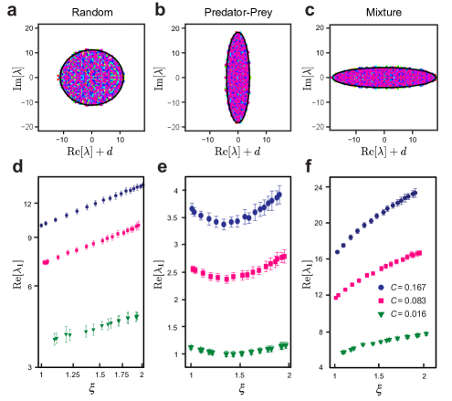
Figure 3: Eigenvalue distributions of 10 community matrices (color) with $-d=-1$ on the diagonal and off-diagonal elements following the random (a), predator-prey (b), and mixture of competition and mutualism interactions (c), respectively. $S=250$, $C=0.25$, $\sigma=1$. The black ellipses are analytical results. Panels a, b, and c were redrawn from [9]. Impact of degree heterogeneity on the stability of ecological systems with random interactions (d), predator-prey (e), and mixture of competition and mutualism interactions (f). The dots represent the results from numerical simulations on 3-modal networks with different connectances. Higher $\text{Re}[\lambda_{1}]$ indicates lower stability. Each error bar represents the standard deviation of 100 independent runs. $S=1200$, $\sigma=1$, and $d=0$. Panel d was drawn in the log-log scale. Panels d, e, and f were redrawn from [272].

May’s result continues to be influential almost five decades later, not because it asserts that ecological systems must be inherently unstable, but rather because it highlights the importance of specific structural characteristics that enable real ecological systems to maintain stability despite their inherent complexity [39]. In other words, nature must adopt some devious and delicate strategies to cope with this stability-complexity paradox.

3.1.2 Impacts of interaction types and correlation

One of the specificity is the existence of well-defined interspecific relationships observed in nature, e.g., predator-prey, competition, mutualism, and a mixture of competition and mutualism. In 2012, by leveraging Sommers’ Ellipical Law [241], Allesina et al. refined May’s result and provided stability criteria for all these interspecific interaction types [9] , as shown in Table 3 and Figure 3a, b, and c. They found remarkable differences between predator-prey interactions, which are stabilizing, but mutualistic and competitive interactions, which are destabilizing. Additionally, the correlation between interaction strengths determines interaction types. Tang et al. therefore incorporated correlation into the stability analysis by deriving a new stability criterion for large ecological systems with random interactions [251] , i.e.,

$$\sigma\sqrt{SC}(1+\rho)-\mu<d,$$ (5)

where $\rho$ and $\mu$ are the overall correlation between pairs of interactions and the mean of the off-diagonal elements in the community matrix M, respectively. The criterion (5) can be viewed as a generalization of those for predator-prey, competition, and mutualism, derived by Allesina et al. [9]. The authors found that the effect of correlation of interaction strengths substantially influences the stability of large food webs (with predator-prey interactions) compared to other network structural properties. Hence, the presence of correlation between interactions of species can significantly influence the locations of the eigenvalues of the community matrix and the resulting stability of ecological systems [9, 37, 149, 251].

3.1.3 Impacts of degree heterogeneity

Many of the “devious strategies” adopted by nature can now be tested with the revised formula as a reference point. For example, one can further study the impact of degree heterogeneity on the stability of ecological systems. Degree heterogeneity measures the variability of the number of interactions associated with each species. Yan et al. found that for ecological systems with random interactions or a mixture of competition and mutualism interactions, increasing the degree of heterogeneity always destabilizes ecological systems [272], see Figure 3d, f. For ecological systems with predator-prey interactions constructed from either simple network models or a realistic food web model (cascade model), high heterogeneity is always destabilizing, yet moderate heterogeneity is stabilizing [271, 272], see Figure 3e. Furthermore, they obtained a stability criterion for large ecological systems with random interactions by considering the factor of degree heterogeneity, i.e.,

$$\sigma\sqrt{(S-1)C\xi}<d,$$ (6)

where $\xi$ denotes the degree heterogeneity. Similarly, Allesina et al. found that broad degree distributions tend to stabilize food webs by approximating the real part of the leading (“rightmost”) eigenvalue of the community matrix [10]. Recently, Baron derived a closed-form expression for the eigenvalue spectrum of a general directed and weighted network [35]. The findings of this study suggest that network heterogeneity appears to be a destabilizing influence in most circumstances, except when the interactions are very asymmetric (e.g., very asymmetric predator-prey interactions). These results are consistent with what were reported by Yan et al. [272].

3.1.4 Impacts of self-regulation

Self-regulation (reflected as negative diagonal elements of the community matrix) is also a key factor for stability in real or random ecological systems. To study the effect of self-regulation on the stability of ecological systems, Barabás et al. derived an analytic approximation of these diagonal elements, i.e.,

$$d_{ii}=-d=-2^{1.5}\text{Re}[\lambda_{1}]$$ (7)

for $i=1,2,\dots,S$, where $\lambda_{1}$ is the leading (“rightmost”) eigenvalue of the community matrix M without self-regulations [30]. Notably, empirical food webs can only achieve stability when the majority of species exhibit strong self-regulation [30]. Even for random ecological systems, attaining stability also requires negative self-regulations for a large amount of species [30]. In addition, Tang et al. investigated the effect of non-constant diagonal on the eigenvalue distribution of the community matrix M [251]. They found that a moderate variance of the diagonal elements minimally affects the distribution of the eigenvalues. Therefore, if the diagonal elements of M follow a moderate-variance distribution with mean satisfying (7), the ecological system will remain locally stable. Nevertheless, when the variance significantly surpasses that of the interspecific interactions, the impact on stability depends on the specific patterns of the diagonal elements. When the self-regulation is stronger for species with fewer interactions, the impact of a considerable variance on stability remains negligible [251].

3.1.5 Impacts of modularity

The stability of ecological systems can also be influenced by network modularity. A modular network can be divided into different modules or subsystems, and the interactions within each subsystem are much more frequent than those between subsystems [180]. The modularity of a network can be defined as

$$Q=\frac{L_{w}-\mathbb{E}[L_{w}]}{L_{w}+L_{b}},$$

where $L_{w}$ is the observed number of interactions within the subsystems, and $L_{b}$ is the number of inter-subsystem interactions. Grilli et al. studied the effect of modularity $Q$ on the stability of ecological systems [114]. They found that modularity exhibits a moderate stabilizing effect when the subsystems have similar sizes and the overall mean interaction strength is negative. In particular, the stabilizing effect becomes stronger for negative correlations. Conversely, anti-modularity is highly destabilizing, except for the case where the overall mean interaction strength is close to zero. The authors further investigated the effect of modularity in food webs through numerical simulations and found that the results remain qualitatively unchanged [114].

3.1.6 Impacts of dispersal

Spatial flows (e.g., exchanges of individuals, energy, and material) among local ecosystems are ubiquitous in nature [206]. Gravel et al. incorporated dispersal, i.e., spatial movement of species among local ecological systems, into the stability analysis of meta-ecological systems [111]. The community matrix M of a meta-ecological system can be expressed as the sum of three matrices, i.e.,

$$\textbf{M}=\textbf{D}+\textbf{Q}+\textbf{K},$$

where D is a diagonal matrix that accounts for intraspecific density dependence, Q is a matrix representing dispersal among patches with diffusion coefficient $q$, and K is a block diagonal matrix that contains the local community matrices (random matrices with $S$ species, connectance $C$, and interspecific interaction strength $\sigma$). By assuming the number of local systems and $S$ are large, the authors obtained the following stability criterion [111]:

$$\sigma\sqrt{C(S-1)}<d+q.$$ (8)

Therefore, the effect of dispersal can promote stability in meta-ecological systems, in which dispersal can move the most of the eigenvalues of the community matrix towards more negative values and shrinks the range of the remaining in proportion to the number of effective patches. Interestingly, Baron et al. discovered that the introduction of dispersal can lead to the Turing-type instability (i.e., the equilibrium point is unstable with respect to disturbances of a finite range of wavelengths) in an ecological system with a trophic structure [36]. While the inclusion of trophic structures often enhances stability in large ecological systems (e.g., food webs) [116, 135], it can lead to a peak in the real part of the maximum eigenvalue of the community matrix in the presence of dispersal, rendering the equilibrium point unstable [36].

3.1.7 Impacts of time delay

Empirical evidence has indicated that species interactions often exhibit time lags, rather than occurring instantaneously [181, 184]. Thus, time delays can hold significant implications for stability and coexistence. Notably, Pigani et al. investigated delay effects on the stability of large ecological systems [200], which can be captured by the following linearized equation:

$$\dot{\textbf{z}}(t)=\textbf{M}\textbf{z}(t)+\textbf{M}_{\text{delay}}\textbf{z}(t-\tau),$$ (9)

where $\textbf{M}_{\text{delay}}$ is the community matrix with delay. For simplicity, the community matrix M is set to $-d_{M}\textbf{I}$ where $d_{M}\geq 0$, which guarantees stability for a sufficiently small community matrix delay. In other words, the current intraspecific interactions are always stabilizing. $\textbf{M}_{\text{delay}}$ is supposed to be a random matrix with a constant diagonal entry $-d_{\text{delay}}\leq 0$ and off-diagonal elements normally distributed with zero mean, standard derivation $\sigma_{\text{delay}}$, and connectance $C_{\text{delay}}$. The authors proved that (9) is stable if all the roots of the characteristic equation, defined as $H(z)=z-\lambda-\lambda_{\text{delay}}e^{-z\tau}$ where $\lambda$ and $\lambda_{\text{delay}}$ are the eigenvalues of M and $\textbf{M}_{\text{delay}}$, respectively, have negative real parts [200]. Importantly, these roots can be solved implicitly as a function of $\tau$, along with the parameters $d_{M}$, $d_{\text{delay}}$, $\sigma_{\text{delay}}$, and $C_{\text{delay}}$. They found that an increasing delay tends to destabilize the system, and if a system is already unstable for $\tau=0$, the delay cannot stabilize the system. Furthermore, the authors determined the critical delay $\tau^{*}$ as the minimum value of $\tau$ above which the system becomes unstable. Finally, distributed delay was considered, i.e., the second term in (9) is modified to $\textbf{M}_{\text{delay}}\int_{0}^{\infty}\exp{\{-\frac{\tau}{\tilde{\tau}}\}}/\tilde{\tau}\textbf{z}(t-\tau)d\tau$, which can be derived from logistic or resource competition models [117]. They found that the system becomes more and more unstable as $\tilde{\tau}$ increases. However, if $\tilde{\tau}$ is large enough, the system eventually goes back to the stable regime [200].

3.1.8 Limitations of model-implicit approaches

May’s approach and the follow-up studies offer a valuable theoretical framework for understanding the stability of ecological networks with various structures. Yet, these model-implicit approaches heavily rely on randomly sampling interactions without an underlying dynamical model, which results in a lack of biologically realistic representation of species interactions. Consequently, the analytical results produced by these approaches are independent from the underlying model from which they are hypothetically derived. While informative, these results may not accurately capture the nuanced and complex interactions that characterize the stability of real ecological systems. One way to enhance this framework is to integrate underlying ecological models into the linear stability analysis, as detailed in the next subsection.

3.2 Model-explicit approaches

The most commonly used model to describe the dynamics of ecological systems is the generalized Lotka-Volterra (GLV) model [49, 162] defined as

$$\dot{x}_{i}(t)=x_{i}(t)\Big{[}r_{i}+\sum_{j=1}^{S}\textbf{A}_{ij}x_{j}(t)\Big{]}$$ (10)

for $i=1,2,\dots,S$, where $r_{i}$ is the intrinsic growth rate of species $i$ and $\textbf{A}\in\mathbb{R}^{S\times S}$ is the interaction matrix whose off-diagonal elements $\textbf{A}_{ij}$ represent the effect that species $j$ has upon species $i$. By assuming the existence of a feasible equilibrium point ${\bf x}^{*}$ (i.e., $x_{i}^{*}\geq 0$ for all species), the community matrix can be computed as $\textbf{M}=\textbf{X}\textbf{A},$ where $\textbf{X}\in\mathbb{R}^{S\times S}$ the diagonal equilibrium matrix such that $\textbf{X}_{ii}=x_{i}^{*}$. Hence, the community matrix can be regarded as the scaled interaction matrix. Similarly to model-implicit approaches, we can investigate the stability properties of the GLV model based the linearized equation (3).

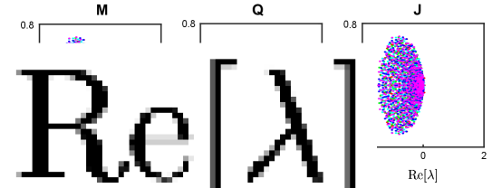
Figure 4: Eigenvalue distributions of the three matrices M, Q, and J. The off-diagonal elements of A are sampled from a normal bivariate distribution with identical marginal $\mu_{A}=5/S$, $\sigma_{A}=5/{\sqrt{S}}$, and correlation $\rho_{A}=-0.5$. The diagonal elements of A are fixed to $\mu_{d}=-1$, while the diagonal elements of X are sampled from a uniform distribution on [0,1]. The two matrices Q and J are defined as $\textbf{Q}=\textbf{X}[(\mu_{d}-\mu_{A})\textbf{I}+\mu_{A}\textbf{1}]$ and $\textbf{J}=\textbf{X}(\mu_{d}\textbf{I}+\textbf{B})$, respectively, such that the bulk of the eigenvalue distributions of M are the same as these of J, and the outlier eigenvalue of M is the same as that of Q. Here, B is a random matrix with zero diagonal elements whose off-diagonal elements have mean zero and variance $\sigma_{A}^{2}$. $S=500$. This figure was redrawn from [100].

3.2.1 Impacts of equilibria

Equilibrium points play a significant role in the local stability analysis of the GLV model, as its community matrix is directly related to the equilibrium points of the system. Gibbs et al. explored the eigenvalue spectrum of the community matrix by assuming that the diagonal equilibrium matrix X and the interaction matrix A are randomly drawn from an arbitrary distribution with positive support and a bivariate distribution, respectively [100]. They proved that the eigenvalue spectrum of the community matrix M consists of a bulk of eigenvalues with mean $\mu_{X}(\mu_{d}-\mu_{A})$ determined by the eigenvalues of the matrix $\textbf{J}=\textbf{X}(\mu_{d}\textbf{I}+\textbf{B})$ and an outlier eigenvalue determined by the largest eigenvalue of the matrix $\textbf{Q}=\textbf{X}[(\mu_{d}-\mu_{A})\textbf{I}+\mu_{A}\textbf{1}]$ (1 is the all-one matrix) such that

$$\lambda_{\text{outlier}}=\mu_{X}[\mu_{d}+(S-1)\mu_{A}],$$

where $\mu_{X}$, $\mu_{d}$, and $\mu_{A}$ represent the mean of the diagonal of X, the diagonal of A, and the off-diagonal of A, respectively, see Figure 4. Based on their finding, the authors concluded that for mutualistic ecological systems, if the interaction matrix is stable, then the community matrix will also be stable [100]. It is important to note that Gibbs et al. made the assumption that the distribution from which the equilibrium is drawn is independent of the interaction matrix, which does not typically hold in reality. Nevertheless, Liu et al. discovered that if the equilibrium point follows a specific distribution related to the elements of the interaction matrix A, Gibbs et al.’s assumption remains valid [157]. Around the same time, Stone demonstrated that for large ecological systems described by the GLV model, the stability of the interaction matrix implies the stability of the community matrix, under the condition that all species have positive equilibria [246].

3.2.2 Impacts of extinction

Extinction is generic in the GLV model with random interactions [38, 88, 197]. Recent studies have highlighted that an equilibrium point of the GLV model is locally stable if and only if all the eigenvalues of the reduced interaction matrix (i.e., the interaction matrix between the species in the surviving sub-community) have negative real parts [31, 38, 53, 246]. Baron et al. focused on the eigenvalue spectrum of the reduced interaction matrix in the GLV model, where the spectrum of the reduced interaction matrix also consists of a bulk set of eigenvalues and an outlier [38]. Importantly, the authors demonstrated that the universality principle holds for the bulk region (i.e., following Ellipse Law) but not for the outlier eigenvalue. The outlier eigenvalue can be solved from the generating functional approach. Prediction of extinction boundary and new equilibrium after a primary extinction were also discussed in [197] and [88], respectively.

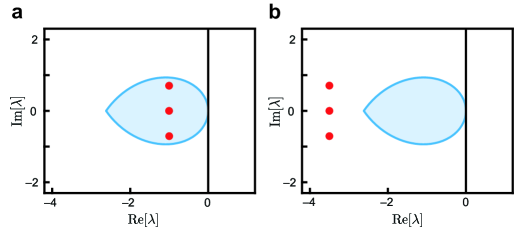
Figure 5: Eigenvalue distributions with time delay, where the blue teardrop-shaped area represents the stability region with time delay. (a) The eigenvalues (represented by red dots) are within the teardrop-shaped area, indicating that the corresponding GLV model with time delay is locally stable. (b) The eigenvalues are outside the teardrop-shaped area, indicating that the corresponding GLV model with time delay is unstable. $\tau=1$. The figure was redrawn from [273].

3.2.3 Impacts of time delay

Similar to Pigani et al.’s work as discussed in Section 3.1.7, Yang et al. investigated the stability of the time-delayed GLV model [273], which is defined as

$$\dot{x}_{i}(t)=x_{i}(t)\Big{[}r_{i}+\sum_{j=1}^{S}\textbf{A}_{ij}x_{j}(t-\tau)\Big{]}.$$ (11)

The linearized equation of the time-delayed GLV model is given by

$$\dot{\textbf{z}}(t)=\textbf{M}_{\text{delay}}\textbf{z}(t-\tau),$$ (12)

where $\textbf{M}_{\text{delay}}=\textbf{X}\textbf{A}$ is the community matrix with delay. For simplicity, X is set to I such that each species has unit abundance. However, the validation of this assumption remains an open problem [273]. They proved that (12) is stable if all the roots of the characteristic equation, defined as $H(z)=z-\lambda_{\text{delay}}e^{-z\tau}$ where $\lambda_{\text{delay}}$ are the eigenvalues of $\textbf{M}_{\text{delay}}$, have negative real parts. This equation implies that all the eigenvalues of $\textbf{M}_{\text{delay}}$ are required to be located in a teardrop-shaped region defined by $\text{Re}[z]<0$ to ensure stability, see Figure 5. Since the distribution of the eigenvalues of $\textbf{M}_{\text{delay}}$ (i.e., the interaction matrix A is this case) with random, mutualistic, or competitive interactions is well-established, it becomes straightforward to estimate $\max{(\text{Re}[z])}$. Based on the theoretical findings, the authors found that time delay plays a critical role in ecological systems, where large delay is often destabilizing, but short delay can considerably enhance community stability ($\tau=0.2$ and 0.5 were used for the small and large time delay in their simulations, respectively) [273].

Similar conclusions were also obtained by Saeedian et al. when investigating the impact of time delay on the emergent stability patterns within the time-delayed GLV model (11) [224]. Significantly, they further determined the existence of a Hopf bifurcation (i.e., the two complex conjugate eigenvalues of the community matrix, with non-zero imaginary part, simultaneously cross the imaginary axis into the right half-plane) at $\tau_{c}$, which is computed as

$$\tau_{c}=\min_{\lambda_{i}\in\lambda(\textbf{M}_{\text{delay}})}\frac{1}{\lambda_{i}}\text{artan}\Bigg{|}\frac{\text{Re}[\lambda_{i}]}{\text{Im}[\lambda_{i}]}\Bigg{|}$$

for the time-delayed GLV model with a large number of species.

3.2.4 Impacts of stochastic noises

Real ecological systems are inherently stochastic with constant external perturbations and internal fluctuations [254]. Krumbeck et al. developed a theoretical framework for the analysis of temporal stability of ecological systems with stochastic noises [148]. They provided analytical predictions for the power spectral density of the stochastic GLV model defined as

$$\dot{x}_{i}(t)=x_{i}(t)\Big{[}r_{i}+\sum_{j=1}^{S}\textbf{A}_{ij}x_{j}(t)\Big{]}+\frac{1}{\sqrt{V}}\eta_{i}(t),$$ (13)

where $V$ is the size of the species living domain, and $\eta_{i}(t)$ are Gaussian noises. The power spectral density is a statistical measure that can capture various aspects of temporal stability (e.g., the height of the spectrum gives information about the magnitude of stochastic fluctuations; the locations of nonzero peaks correspond to quasi-cyclic signals; a peak at zero indicates baseline wander). Specifically, the authors utilized the linearized equation of the stochastic GLV model (13), i.e.,

$$\dot{\textbf{z}}(t)=\textbf{M}\textbf{z}(t)+\boldsymbol{\zeta}(t),$$ (14)

where $\boldsymbol{\zeta}(t)$ is a vector of Gaussian white noises with correlation matrix B. The power spectral density of fluctuations $\Psi(\omega)$ in the frequency domain can be computed as

$$\Psi(\omega)=(\textbf{M}-i\omega\textbf{I})^{-1}\textbf{B}(\textbf{M}^{\top}+i\omega\textbf{I})^{-1},$$

where $i$ here is the imaginary number. They showed that different network structures (random, mutualistic, and competitive) have unique signatures in the spectrum of fluctuations. They further investigated the effect of trophic structures and identified a gap in the power spectral density, which indicates that high-level trophic structures contribute to enhanced long-term temporal stability [148].

3.2.5 Impacts of evolved system size

Previous work on the linear stability of the GLV model is concerned with ecological systems of predetermined and fixed sizes. Galla explored the stability of ecological systems with evolved system size using methods from statistical mechanics and the theory of disordered systems [96, 163, 171]. Specifically, he exploited generating functionals to derive the effective dynamics for the GLV model (with $r_{i}=1$) computed as

$$\dot{x}(t)=x(t)\Big{[}1-x(t)+\mu_{A}M(t)+\rho_{A}\sigma_{A}^{2}\int_{0}^{t}G(t,t{{}^{\prime}})x(t{{}^{\prime}})dt{{}^{\prime}}+\eta(t)\Big{]},$$ (15)

where $M(t)$ is the average species concentration, $G(t,t{{}^{\prime}})$ is the response function, and $\eta(t)$ is the Gaussian noise. As described previously, $\mu_{A}$, $\sigma_{A}$ and $\rho_{A}$ are the mean, standard derivation, and correlation of the off-diagonal elements of the interaction matrix A, respectively. The effective process characterizes the dynamics of a single representative species, denoted by $x(t)$, and captures the statistical behaviors of the ecological system. The linearized effective dynamics can be computed as

$$\dot{z}(t)=x^{*}\Big{[}-z(t)+\rho_{A}\sigma_{A}^{2}\int_{0}^{t}G(t,t{{}^{\prime}})z(t{{}^{\prime}})dt{{}^{\prime}}+v(t)+\zeta(t)\Big{]},$$ (16)

where $z(t)$ denotes fluctuations about the equilibrium $x^{*}$, $v(t)$ is the deviation of the noise in the effective process, and $\zeta(t)$ is the Gaussian white noise of unit amplitude. By performing Fourier transform with a focus on the long-time behavior of perturbations ($\omega=0$), the author established that the GLV model has stable equilibrium points in the limit of large population for

$$\sigma_{A}<\sqrt{\frac{2}{(1+\rho_{A})^{2}}}.$$ (17)

This result implies that predator-prey relationships enhance stability, while variability in species interactions promotes instability [96], which aligns with prior findings as reported in [251, 272].

Poley et al. applied Galla’s approach to analyze the stability of the GLV model with hierarchical interactions [205] defined as

$$\dot{x}_{i}^{a}(t)=x_{i}^{a}(t)\Big{[}r_{i}^{a}+\sum_{b=1}^{B}\sum_{j=1}^{S^{b}}\textbf{A}_{ij}^{ab}x_{j}^{b}(t)\Big{]}$$ (18)

for $i=1,2,\dots,S^{a}$, where $B$ is the total number of local systems, and $a,b=1,2,\dots,B$ denote the indices of the local systems with the associated system size $S^{a}$ and $S^{b}$. Their findings indicate that a strong hierarchical structure is stabilizing but reduces diversity within the effective dynamics of the GLV model [205]. Similarly, Sidhom and Galla adapted Galla’s approach to study the GLV model with nonlinear feedback [231] defined as

$$\dot{x}_{i}(t)=x_{i}(t)\Big{[}r_{i}+g\big{(}\sum_{j=1}^{S}\textbf{A}_{ij}\,x_{j}(t)\big{)}\Big{]}$$ (19)

for $i=1,2,\dots,S$, where the function $g(u)=\frac{2au}{a+2|u|}$ denotes the nonlinear feedback ($a$ is the saturation parameter). This form of feedback was initially introduced to describe the predator’s growth rate when interacting with prey. It is plausible that the benefits from extra prey will eventually saturate as prey numbers become large. The authors concluded that the stability and diversity of ecological systems improves with the introduction of nonlinear feedback [231].

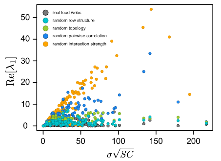
Figure 6: Stability of real and permuted food webs in relation to complexity. These permuted food webs were constructed from real food webs by removing some non-random features, namely the row structure, topology, pairwise correlation, and interaction strength. The more the “rightmost”eigenvalues, i.e., $\text{Re}[\lambda_{1}]$, close to zero, the more stable of the food webs (because the diagonal elements of the community matrix are set to zero). This figure was redrawn from [128].

3.2.6 Applications to real ecological systems

Last but not least, while the stability analysis of random ecological systems offers powerful insights for the study of ecological dynamics and the understanding of how species interactions shape the stability and diversity of ecological communities, empirically applying the theory to real ecological systems poses a formidable challenge [79, 89, 128, 178, 179, 276, 277]. Notably, Jacquet et al. performed the local stability analysis of 116 real food webs sampled worldwide from marine, freshwater, and terrestrial habitats using the GLV model [128]. The community matrix M was constructed by multiplying the interaction matrix A with species biomass for each food web. The interaction coefficients of A can be translated from the parameters of the corresponding Ecopath model, a trophic model that provides accurate representation of feeding interactions within food webs [71]. The authors then measured the stability of food webs using the real part of the dominant eigenvalue of the community matrix M. Using randomization tests, they found that negative correlation between interaction strengths with high frequency of weak interactions is a strong stabilizing property in real food webs, see Figure 6. Their findings reveal that empirical food webs exhibit some non-random characteristics that lead to the absence of a complexity–stability relationship [128].

4 Sign stability analysis

The notion of sign stability is of particular interest for ecology, economics, chemistry, and engineering [73, 91, 133, 161, 166, 208, 274, 275]. In an ecological system, the community matrix ${\bf M}$ (or the interaction matrix A) associated with certain models (e.g., the GLV model) might be only known qualitatively in the sense that the signs of the elements $\textbf{M}_{ij}$ can be determined with reasonable confidence, but the actual magnitudes may be very difficult to determine, see Figure 7. Such matrices are often referred to as sign matrices. A sign matrix ${\bf M}$ is called sign stable (or sign semi-stable) if each of its eigenvalues has negative real part (or non-positive real part, respectively) for all numerical matrices of the same sign pattern [132, 133, 169, 208, 270].

4.1 Characterizations of sign stable matrices

A sign matrix ${\bf M}\in\mathbb{R}^{S\times S}$ is sign semi-stable if and only if the following conditions are all satisfied: (i) $\textbf{M}_{ii}\leq 0$ for $i=1,2,\dots,S$; (ii) $\textbf{M}_{ij}\textbf{M}_{ji}\leq 0$ for $i,j=1,2,\dots,S$ and $i\neq j$; (iii) there exists no elementary cycle of length $k\geq 3$ in the digraph generated by M [169, 208]. It is also known that if $\textbf{M}_{ii}<0$ for $i=1,2,\dots,S$, then (ii) and (iii) are necessary and sufficient for ${\bf M}$ to be sign stable. Quirk and Ruppert further claimed that (i)-(iii) as well as (iv) $\textbf{M}_{ii}<0$ for some $i$ and (v) $\text{det}(\textbf{M})\neq 0$ are both necessary and sufficient for ${\bf M}$ to be sign stable [208]. However, this was proved to be incorrect later by Jeffries et al. [132]. Later on, Yamada demonstrated that such an exceptional case is very rare and proved that the conditions (i)-(v) proposed by Quirk and Ruppert is actually necessary and sufficient for a system to be generically sign stable, i.e., sign stable for almost all parameter values except for some pathological cases with measure zero [270].

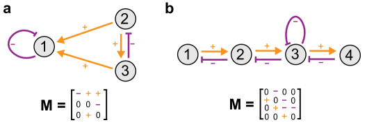
Figure 7: Examples of signed ecological networks and their corresponding sign community matrices. (a) Self-regulated species 1 forms a commensal relationship with each species within the prey-predator pair of 2 and 3. (b) Linear trophic chain in which each successive species is preyed upon the subsequent one and species 3 is self-regulated. This figure was redrawn from [161].

Quirk and Ruppert’s conditions (i)-(v) can be translated into ecological terms to provide a comprehensive characterization of sign stable patterns [161]. According to (i) and (iv), a sign stable ecological system should not include self-promoting species and must have at least one species with self-regulation. Condition (ii) necessitates the absence of both competitive and mutualistic relations. Condition (iii) states that there are no closed directed cycles with more than two edges in the network structure. Finally, condition (v) requires that the digraph generated by M must include a specific number of non-overlapping directed cycles that encompass all the nodes.

Jeffries et al. introduced two additional conditions, distinct from (iv) and (v), called the coloring and matching conditions [132]. The two conditions, combined with (i)-(iii), are necessary and sufficient for sign stability. Let $\mathcal{R}_{M}=\{i\text{ }|\text{ }\textbf{M}_{ii}\neq 0\}$. An $\mathcal{R}_{M}$-coloring of an undirected graph is a partition of its nodes into two sets, black and white, such that each node in $\mathcal{R}_{M}$ is black (one of which can be empty), no black node has exactly one white neighbor, and each white node has at least one white neighbor. The coloring condition then states that in every $\mathcal{R}_{M}$-coloring of the undirected graph generated by M, all nodes are black. Additionally, a $(\mathcal{V}\sim\mathcal{R}_{M})$-complete matching in an undirected graph is a set $\mathcal{M}$ of disjoint edges such that an exact cover of the node set can be obtained using the pairs in $\mathcal{M}$ and certain singletons from $\mathcal{R}_{\mathcal{M}}$. The matching condition then asserts that the undirected graph generated by M admits a $(V\sim\mathcal{R}_{M})$-complete matching. However, the ecological systems characterized by Quirk and Ruppert [208] or Jeffries et al. [132] are not readily observable in nature.

4.2 Applications to ecological systems

The notion of sign stability has been applied to various ecological systems through different approaches. Dambacher et al. introduced two qualitative metrics – weighted feedback and weighted determinants based on the Hurwitz criterion [77], which can be recast into two conditions: (i) the coefficients of the characteristic equation of M must have the same sign; (ii) the corresponding Hurwitz determinants must all be positive. The two metrics offer a practical mean to identify the relative degree to which stable parameter space can be constrained based on system structure and complexity. Remarkably, Haraldsson et al. utilized the weighted feedback and weighted determinants to investigate the sign stability of social-ecological systems, which is an important tool to understand human-nature relations [120].

Moreover, Allesina and Pascual studied the sign stability of random and empirical food webs through a fairly intuitive approach [11]. Given a community matrix M (either randomly generated or empirical), first determine the stability based on its eigenvalues. If it is stable (in terms of $\text{Re}[\lambda(\textbf{M})]\leq 0$), generate 100 matrices that have the same sign pattern with random magnitude. Lastly, measure the percentage of the random generated matrices that are stable. The percentage can tell whether the stability is due to a particular combination of coefficients or the sign pattern of the network itself. Based on this approach, the authors demonstrated that predator-prey interactions can promote stability, highly robust to perturbations of interaction strength, in real ecological systems [11].

5 Diagonal stability analysis

The notion of diagonal stability was first introduced by Volterra in the 1930s [263]. It has been particularly useful for the stability analysis of ecological systems and other networked systems [29, 34, 46, 50, 136, 137, 188, 248]. A matrix A is called diagonally stable if there exists a diagonal matrix ${\bf P}\succ 0$ that renders

$$\textbf{A}^{\top}\textbf{P}+\textbf{P}\textbf{A}=-\textbf{Q}\prec 0.$$

We use the notation $\mathcal{D}(\textbf{P})$ for the class of diagonally stable matrices. The positive diagonal matrix P is often called Volterra multiplier in literature [212]. In many cases, the necessary and sufficient conditions for the Lyapunov stability of nonlinear systems are also the necessary and sufficient conditions for the diagonal stability of a certain matrix associated to the nonlinear system. This matrix naturally captures the underlying network structure of the nonlinear dynamical system.

Diagonal stability has been successfully applied to various types of dynamical systems [8, 142, 164, 245, 247, 269]. It has nice “structural consequences.” For example, the principal sub-matrices of a diagonally stable matrix are also diagonally stable, implying that all the corresponding “principal sub-systems” of a given diagonally stable system are diagonally stable [137]. In this section, we begin by introducing the theoretical framework for determining the Lyapunov stability of the GLV model via diagonal stability analysis. Subsequently, we delve into the characterizations of diagonal stability of the interaction matrix that is associated with special interconnection or network structures, which offer an effective mean of determining the stability of ecological systems.

5.1 Lyapunov stability of the GLV model

Before talking about the stability of the GLV model, we first introduce the notion of Persidskii-type systems. Persidskii-type systems are typical examples that admit diagonal-type Lyapunov functions [86, 85, 196, 203]. We need to introduce a few concepts to define Persidskii-type systems. A function $\textbf{f}:\mathbb{R}^{S}\to\mathbb{R}^{S}:\textbf{x}\mapsto\textbf{f}(\textbf{x})$ is called diagonal if, the $i$th component of f, i.e., $f_{i}$, is a function of $x_{i}$ alone. A function $f:\mathbb{R}\to\mathbb{R}$ is said to be in sector $[l,u]$ if $\forall x\in\mathbb{R}$, $f(x)$ lies between $lx$ and $ux$, i.e.,

$$(f(x)-ux)(f(x)-lx)\leq 0.$$

For example, sector $[-1,1]$ means $|f(x)|\leq|x|$. Sector $[0,\infty]$ means $f(x)$ and $x$ always have same sign. The class of infinite sector nonlinear functions $\mathcal{S}$ is defined to be functions in sector $[0,\infty]$ that satisfy $\int_{0}^{x}f(\tau)d\tau\to\infty$ as $|x|\to\infty$. Typical examples of infinite sector nonlinear functions are $f(x)=x$, $f(x)=x^{3}$, and $f(x)=\tanh(x)$ [137]. A dynamic system $\dot{\textbf{x}}(t)=\textbf{f}(\textbf{x}(t))$ with $\textbf{x}(t)\in\mathbb{R}^{S}$ and $\textbf{f}:\mathbb{R}^{S}\to\mathbb{R}^{S}$ is said to be of Persidskii-type if it has the following form:

$$\dot{x}_{i}(t)=\sum_{j=1}^{S}\textbf{A}_{ij}f_{j}\big{(}x_{j}(t)\big{)}$$ (20)

for $i=1,2,\dots,S$, where $f_{j}\in\mathcal{S}$ for all $j=1,2,\dots,S$. In other words, f is diagonal and $f_{j}$ is in the class of infinite sector nonlinear functions. Note that (20) can be used to describe a wide range of complex networked systems, where $\textbf{A}_{ij}$ capture the weighted wiring diagram.

For Persidskii-type systems, we can introduce a diagonal-type Lyapunov function of the following form:

$$V({\bf x})=\frac{1}{2}\sum_{i=1}^{S}p_{i}\int_{0}^{x_{i}}f_{i}(\tau)d\tau,$$

where $p_{i}$ denotes the $i$th diagonal of P. The equilibrium point $\textbf{x}^{*}={\bf 0}$ of the Persidskii-type system is globally asymptotically stable (in the sense of Lyapunov) if $\textbf{A}\in\mathcal{D}(\textbf{P})$. This can be seen by computing $\dot{V}({\bf x})$ along the trajectory of (20), yielding

$$\dot{V}(\textbf{x})=\textbf{f}^{\top}(\textbf{x})(\textbf{A}^{\top}\textbf{P}+\textbf{P}\textbf{A})\textbf{f}(\textbf{x}).$$

Since f is diagonal and $f_{j}\in\mathcal{S}$, if $\textbf{A}\in\mathcal{D}(\textbf{P})$, therefore $\dot{V}(\textbf{x})$ is negative definite. Moreover, the functions $f_{i}\in\mathcal{S}$ ensure the radial unboundedness of $V(\textbf{x})$. Hence, according to Lyapunov’s theorems of stability, $\textbf{x}^{*}={\bf 0}$ is globally asymptotically stable (in the sense of Lyapunov).

By assuming the existence of a non-trivial equilibrium point ${\bf x}^{*}$ (i.e., $x_{i}^{*}>0$ for all species) and defining

$$z_{i}(t)=\log\frac{x_{i}(t)}{x_{i}^{*}}\quad\text{and}\quad g_{j}\big{(}z_{j}(t)\big{)}=x_{j}^{*}(e^{z_{j}(t)}-1),$$

we can bring the GLV model (10) into the form of Persidskii-type dynamics:

$$\dot{z}_{i}(t)=\sum_{j=1}^{S}\textbf{A}_{ij}\,g_{j}\big{(}z_{j}(t)\big{)},$$

which admits the following diagonal-type Lyapunov function:

$$V({\bf z})=\sum_{i=1}^{S}p_{i}\int_{0}^{z_{i}}g_{i}(\tau)d\tau\quad\text{or}\quad V({\bf x})=\sum_{i=1}^{S}p_{i}\left[x_{i}-x_{i}^{*}-x_{i}^{*}\log\frac{x_{i}}{x_{i}^{*}}\right].$$

Using the above diagonal-type Lyapunov function, Goh first proved that for the GLV model (10), if the interaction matrix A is diagonally stable, then the non-trivial equilibrium point $\textbf{x}^{*}$ in the positive orthant is globally asymptotically stable (in the sense of Lyapunov) [107]. Therefore, diagonal stability allows the GLV model to lie in the unique fixed-point phase, as depicted by Bunin [57]. Here, we provide an example of a 3-by-3 diagonally stable matrix and the corresponding vector field plot of the GLV model, see Figure 8. Clearly, the non-trivial equilibrium point in the positive orthant is globally asymptotically stable.

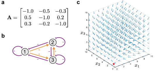
Figure 8: Example of a diagonally stable matrix. (a) Diagonally stable interaction matrix A. It is easy to check that the eigenvalues of $(\textbf{A}+\textbf{A}^{\top})/2$ are all negative. (b) Corresponding ecological network associated with A. (c) Vector field plot of the corresponding GLV model with the non-trivial equilibrium point indicated by the red star.

The diagonal stability analysis has been applied to analyze the stability of various GLV-derived models. Following Goh’s findings, Wörz-Busekros offered a sufficient condition for the global stability of the GLV model with continuous-time delay via diagonal stability analysis [268]. Later on, Beretta and Takeuchi considered the global asymptotic stability of diffusion models with multiple species heterogeneous patches, in which each patch is governed by the GLV model with continuous-time delay [43]. Concurrently, Beretta and Solimano generalized the Wörz-Busekros’s outcome by considering a non-negative linear vector function of the species [42]. In addition, Kon exploited the diagonal stability theory to determine the stability of the GLV model with an age structure [144]. The notion of diagonal stability was further applied to more general ecological models such as Kolmogorov systems [126], where the GLV model is encompassed as a specific instance. Significantly, the stability properties of many quasi-polynomial dynamical systems, often used to represent many biochemical processes, can be studied through an equivalent GLV model that has a much simpler form [122, 173]. This is based on the fact that the former can be transformed into the latter with some appropriate changes of variables.

5.2 Characterizations of diagonally stable matrices

A general characterization of the diagonally stable interaction matrix in the GLV model remains elusive for more than three species [76, 159], though there exist efficient optimization-based algorithms to numerically check if a given matrix is diagonally stable, e.g., polynomial-time interior point algorithms [55]. In cases where the dimension is three or less, the diagonal stability of A can be determined by examining the signs of its principal minors [76]. For high-dimensional matrices under very special structural assumptions, one can derive necessary and sufficient conditions for diagonal stability. For example, if A is Metzler (i.e., $\textbf{A}_{ij}\geq 0\text{ for }i\neq j$), then A is diagonally stable if and only if all principal minors of $-\textbf{A}$ are positive [45]. More special examples are discussed in [212]. Moreover, there are approaches which can reduce the problem of determining whether $\textbf{A}\in\mathbb{R}^{S\times S}$ is diagonally stable into two simultaneous problems of $(S-1)\times(S-1)$ matrices, but the method becomes intractable for large $S$ [212].

Grilli et al. imposed a condition of negative definiteness on A (i.e., all the eigenvalues of $\textbf{A}+\textbf{A}^{\top}$ are negative) to ensure the diagonal stability of A for studying the feasibility and coexistence of large random ecological systems [112]. It is known that a negative definite matrix is also diagonally stable, and the condition is much easier to verify and characterized for random matrices. Later on, Gibbs et al. [100] estimated the “rightmost” eigenvalue of $(\textbf{A}+\textbf{A}^{\top})/2$ with random interactions and proved that if

$$\mu_{d}+\sqrt{2S\sigma_{A}^{2}(1+\rho_{A})}<0,$$ (21)

then A is diagonally stable, where $\mu_{d}$ is the mean of the diagonal elements of A, and $\sigma_{A}^{2}$ and $\rho_{A}$ are the variance and correlation of the off-diagonal elements of A.

Recently, necessary and sufficient diagonal stability conditions for matrices associated with special interconnection or network structures were studied [19, 20, 21, 22, 235, 264]. If an ecological system described by the GLV model exhibits these network structures, it will be effective and efficient to determine its Lyapunov stability through the diagonal stability of the interaction matrix A. We review these network structures as follows.

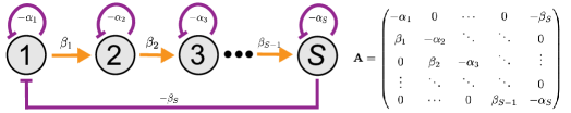
Figure 9: Negative feedback cyclic structure with the corresponding interaction matrix A, where $\alpha_{i}>0$, $\beta_{i}>0$ for $i=1,2,\dots,S$.

5.2.1 Negative feedback cyclic structure

In the negative feedback cyclic structure, the intermediate species play a facilitating role for the subsequent species, while the final species exerts inhibitory effects on the initial species, see Figure 9. It has been shown that the interaction matrix A is Hurwitz, i.e., $\text{Re}[\lambda(\textbf{A})]<0$, if it satisfies the so-called secant criterion [253, 257, 267], i.e.,

$$\frac{\beta_{1}\beta_{2}\cdots\beta_{S}}{\alpha_{1}\alpha_{2}\cdots\alpha_{S}}<\left[\sec\left(\frac{\pi}{S}\right)\right]^{S}.$$ (22)

When $\alpha_{i}$ are equal, the secant criterion (22) is also necessary for A to be Hurwitz. Surprisingly, this secant criterion derived for linear stability is also a necessary and sufficient condition for diagonal stability of the corresponding class of matrices [21].

Note that a simple necessary condition for A to be diagonal stable is that all the diagonal elements $\textbf{A}_{ii}$ be negative. Since scaling the rows of A by positive constants does not change its diagonal stability, one can safely assume $\textbf{A}_{ii}=-1$. Moreover, a reducible matrix A can always be transformed into an upper-triangle form with a suitable permutation, and permutation does not change diagonal stability. Considering these two points, the secant criterion can be further generalized as follows [19]. Any matrix A that can be transformed via a suitable permutation P to the form of

$$\textbf{P}\textbf{A}\textbf{P}^{\top}=\begin{pmatrix}-1&0&\cdots&0&-\tilde{\beta}_{S}\\ \tilde{\beta}_{1}&-1&\ddots&\ddots&0\\ 0&\tilde{\beta}_{2}&-1&\ddots&\vdots\\ \vdots&\ddots&\ddots&\ddots&0\\ 0&\cdots&0&\tilde{\beta}_{S-1}&-1\end{pmatrix}$$

is diagonally stable if and only if $|\gamma|\Phi(\text{sgn}(\gamma),S)<1$ where $\gamma=\tilde{\beta}_{1}\tilde{\beta}_{2}\cdots\tilde{\beta}_{S}\neq 0$ is the cycle gain and $\Phi(\text{sgn}(\gamma),S)=\cos^{S}(\pi/S)$ for $\gamma<0$; $1$ for $\gamma>0$.

5.2.2 Cactus structure

Arcak further generalized the secant criterion to multiple cycles when the weighted digraph of the interaction matrix A, denoted as $G(\textbf{A})$, possesses a “cactus” structure, i.e., any pair of distinct simple cycles have at most one common node [19]. Apparently, the negative feedback cyclic structure corresponds to a single cycle and is just a special case of the cactus structure. The digraph $G(\textbf{A})$ is defined to represent the off-diagonal entries of A that has $S$ nodes and there is a directed edge $(j\to i)$ with weight $\textbf{A}_{ij}$ if and only if $\textbf{A}_{ij}\neq 0$. Self-loops corresponding to the diagonal entries $\textbf{A}_{ii}$ are excluded from $G(\textbf{A})$.

Arcak made two assumptions about A without loss of generality: (i) $\textbf{A}_{ii}=-1$ for $i=1,\dots,S$; (ii) $G(\textbf{A})$ is strongly connected, or equivalently, A is irreducible. Arcak then defined an undirected graph for describing which cycles of the digraph $G(\textbf{A})$ intersect. Subsequently, he constructed a spanning tree in the undirected graph and simultaneously assigned directions to its edges to create an arborescence, i.e., a digraph in which every node can be reached from the root by one and only one path, see Figure 10a, b, c. Using the hierarchy of the cycles of $G(\textbf{A})$ established by this arborescence presentation, he sequentially generated dinequalities for the gains of each simple cycle.

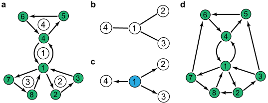
Figure 10: Cactus and connected circle structures. (a) Digraph $G(\textbf{A})$ corresponding to the matrix A with simple cycles $\{1,4,1\},\{1,2,3,1\},\{1,7,8,1\}$, and $\{4,5,6,4\}$ labeled as 1, 2, 3 and 4, respectively. Note that any pair of the cycles have at most one common node. (b) Undirected graph that describes which cycles in $G(\textbf{A})$ intersect. (c) Arborescence constructed on the undirected graph in (b) according to the broadcasting algorithm with cycle 1 selected as the root (shown in cyan). (d) Digraph with the connected circle structure where any pair of the cycles have at most one common edge or one common node. Panels a, b, c were redrawn from [19].

Consider there are $l$ simple cycles in $G(\textbf{A})$. The length of cycle $j$ is denoted as $n_{j}$ for $j=1,2,\dots,l$. Define $\mathcal{I}_{j}=\{i_{j}^{(1)},i_{j}^{(2)},\dots,i_{j}^{(n_{j})}\}$ and $J_{i}=\{1\leq j\leq l\text{ }|\text{ }i\in\mathcal{I}_{j}\}$ as the set of nodes traversed by cycle $j$ and the set of cycles that node $i$ belongs to, respectively. Denote $\gamma_{j}$ as the gain for cycle $j$. Then the stability condition can be summarized as follows: the interaction matrix A satisfying the above two assumptions (i-ii) is diagonally stable if and only if there exist constants $\theta_{j}^{(i)}>0$ such that

$$\begin{cases}\prod_{i\in\mathcal{I}_{j}}\theta_{j}^{(i)}>|\gamma_{j}|\Phi(\text{sgn}(\gamma_{j}),n_{j})\text{ for }j=1,2,\dots,l\\ \sum_{j\in\mathcal{J}_{i}}\theta_{j}^{(i)}=1\text{ for }i=1,2,\dots,S\end{cases}.$$ (23)

Arcak then outlined a systematic procedure for constructing Lyapunov functions based on the above stability condition. Notably, he illustrated the procedure with the GLV model for ecological systems [19].

Later on, Wang and Nešić extended the small gain condition to a more general circle structure called connected circles, where each pair of distinct simple cycles have at most one common edge or a common node [264], see Figure 10d. In addition to the two assumptions (i) and (ii) made by Arcak, the authors further assumed that (iii) A has non-negative off-diagonal elements. Define $\mathcal{L}_{j}=\{e_{j}^{(1)},e_{j}^{(2)},\dots,e_{j}^{(n_{j}-1)}\}$ as the set of edges traversed by cycle $j$. Then the stability condition can be modified as follows: the interaction matrix A satisfying the above three assumptions (i-iii) is diagonally stable if and only if there exist constants $\theta_{j}^{(i)}>0$ such that

$$\begin{cases}\prod_{i\in\mathcal{I}_{j}}\theta_{j}^{(i)}>\gamma_{j}\text{ for }j=1,2,\dots,l\\ \sum_{j\in\mathcal{J}_{i}}\theta_{j}^{(i)}=1\text{ for }i=1,2,\dots,S\end{cases},$$ (24)

where $\gamma_{j}=\prod_{(p,q)\in\mathcal{L}_{j}}\textbf{A}_{pq}$ is the gain for cycle $j$.

5.2.3 Rank-one structure

Recently, Simpson-Porco and Monshizadeh explored necessary and sufficient conditions for the diagonal stability of A with a rank-one network structure [235] defined as

$$\textbf{A}=-\textbf{D}+\textbf{S},$$

where $\textbf{D}=\text{diag}(d_{1},d_{2},\dots,d_{S})$ is a positive diagonal matrix, and $\textbf{S}=\textbf{x}\textbf{y}^{\top}$ is a rank-one matrix for some x, $\textbf{y}\in\mathbb{R}^{S}$. Suppose that y is a non-negative vector. The authors proved that the interaction matrix A with rank-one structure is diagonally stable if and only if

$$\sum_{i=1}^{S}\frac{1}{d_{i}}[x_{i}y_{i}]_{+}<1,$$ (25)

where $x_{i}$ and $y_{i}$ are the $i$th elements of x and y, respectively, and $[\cdot]_{+}=\max{(\cdot,0)}$ is the maximum operator with respect to zero. Significantly, they provided a theoretical stability analysis of automatic generation control in an interconnected nonlinear power system based on the above condition. While the rank-one structure may not naturally occur in real ecological networks, it might be useful in synthetic ecological networks or specific ecological scenarios.

6 D-stability analysis

The notion of D-stability was originally introduced by Arrow and McManus [24] and Enthoven and Arrow [90] in the late 1950s. D-stability can be considered as a weaker version of diagonal stability, see Figure 11. A matrix A is called D-stable if for any positive diagonal matrix X, the matrix XA is stable (in terms of $\text{Re}[\lambda(\textbf{X}\textbf{A})]\leq 0$). Clearly, the definition of D-stability is particularly relevant to the GLV model, where its community matrix is represented as $\textbf{M}=\textbf{X}\textbf{A}$. In this section, we first investigate the characterizations of D-stable matrices and then discuss existing results regarding D-stability in the context of the GLV model.

6.1 Characterizations of D-stable matrices

Explicitly characterizing D-stable matrices is only known for dimension less than or equal to four [159]. For example, a matrix $-\textbf{A}\in\mathbb{R}^{4\times 4}$ is D-stable if and only if all the principal minors of A are positive and $f(x,y,z)>0$ for all positive $x$, $y$, and $z$, where

$$f(x,y,z)=E_{1}(\textbf{D}\textbf{A})E_{2}(\textbf{D}\textbf{A})E_{3}(\textbf{D}\textbf{A})-E_{3}(\textbf{D}\textbf{A})^{2}-\textbf{E}_{1}(\textbf{D}\textbf{A})^{2}E_{4}(\textbf{D}\textbf{A}),$$

and $\textbf{D}=\text{diag}(1,x,y,z)$. Here, $E_{i}(\cdot)$ denotes the sums of the order $i$ principal minors of a given matrix. However, the problem becomes highly challenging as the dimension grows larger [50, 100, 159, 212]. Nonetheless, numerous sufficient conditions have been proposed [134, 153, 191]. Some of the better-known ones are:

• If A is diagonally stable, then it is D-stable [24]. In fact, it is essentially the condition that Arrow and McManus offered.

• If A is Metzler (i.e., $\textbf{A}_{ij}\geq 0$ for $i\neq j$) and all the principal minors of $-\textbf{A}$ are positive, then it is D-stable [92].

• If there exists a positive diagonal matrix D such that $-\textbf{A}\textbf{D}=\textbf{B}$ satisfies $\textbf{B}_{ii}>\sum_{j\neq i}|\textbf{B}_{ij}|$ for $i=1,2,\dots,S$, then A is D-stable [209]. The matrix $-\textbf{A}$ is referred to as quasi-dominant diagonal.

• If A is triangular with $\textbf{A}_{ii}<0$ for $i=1,2,\dots,n$, then it is D-stable [134]. This is the most straightforward condition for D-stability.

• If A is sign stable, then it is D-stable [134].

• The element-wise product of P and A is stable for each positive definite symmetric matrix P [210].

Regrettably, none of these conditions is necessary for D-stability. More sufficient conditions can be found in [134].

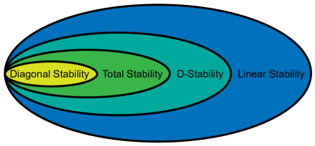
Figure 11: Schematic containment plot of matrix stability notions. Detailed proofs of the relations among these stability notions can be found in [159]. This figure was redrawn from [224].

6.2 Results with the GLV model

Here, we present a series of findings and speculation regarding D-stability in the context of analyzing the GLV model. Chu offered a solvable Lie algebraic condition for the equivalence of four stability notions – linear stability, D-stability, total stability (defined in Section 7), and diagonal stability for the GLV model [72]. Given a Lie algebra $\mathbb{L}$, let’s define the inductive sequence as

$$\mathbb{L}^{(0)}=\mathbb{L},\quad\mathbb{L}^{(i+1)}=\{\textbf{A}\textbf{B}-\textbf{B}\textbf{A}\text{ }|\text{ }\textbf{A},\textbf{B}\in\mathbb{L}^{(i)}\}.$$

The Lie algebra $\mathbb{L}$ is referred to as solvable if there exists a positive integer $k>0$ such that $\mathbb{L}^{(k)}=\{\textbf{0}\}$. The author proved that given the GLV model (10), if the two matrices, defined as $(\textbf{A}+\textbf{A}^{\top})/2$ and $(\textbf{A}-\textbf{A}^{\top})/2$, generate a solvable Lie algebra, then the linear stability, D-stability, total stability, and diagonal stability of the interaction matrix A are equivalent. Moreover, although diagonal stability is not equivalent to Lyapunov stability in general, based on intensive numerical simulations, Rohr et al. conjectured that for mutualistic ecological systems captured by the GLV model, if the interaction matrix A is stable (in the sense of Lyapunov), then A is D-stable [215]. This conjecture has an important consequence for modeling mutualistic ecological systems with the GLV model, implying that if A is stable (in the sense of Lyapunov), any feasible equilibrium point is globally stable, corresponding to the unique fixed-point phase, as illustrated by Bunin [57]. Similarly, Gibbs et al. observed that large random matrices are D-stable almost surely (i.e., the set of positive diagonal matrices leading to instability has measure zero), so feasible unstable equilibrium points are very unlikely for the GLV model with random interactions [100].

7 Total Stability

The notion of D-stability is also closely linked to another stability notion termed total stability. A matrix A is called totally stable if any principal sub-matrix of A is D-stable [123, 208]. Any principal sub-matrix of a totally stable matrix is also totally stable. In addition, total stability is a stronger notion compared to D-stability, but is weaker than diagonal stability, as illustrated in Figure 11. Consequently, any totally stable matrix is inherently D-stable, and the class of totally stable matrices is closed under transposition and multiplication by a positive diagonal matrix. This implies that total stability holds simultaneously for both the interaction matrix A and the community matrix M of the GLV model [158]. A direct way to characterize a totally stable matrix is to check the D-stability of all its principal sub-matrices, which is computationally expensive. However, explicit characterizations are only known for $S\leq 3$ [158, 160], similar to diagonal stability and D-stability. A necessary condition of total stability is that all the principal minors of A of odd orders are negative, while those of even orders are positive [158]. Here, we provide an example of a 3-by-3 totally stable matrix that is not diagonally stable as follows (borrowed from [158]):

$$\textbf{A}=\begin{bmatrix}-1&-0.3&-2\\ -0.95&-1&-1.92\\ -0.49&-0.495&-1\end{bmatrix}.$$

It can be shown that all principal sub-matrices of A are D-stable. For example, the real parts of the eigenvalues of the following product

$$\textbf{X}\textbf{A}=\begin{bmatrix}x_{1}^{*}&0\\ 0&x_{2}^{*}\end{bmatrix}\begin{bmatrix}-1&-0.3\\ -0.95&-1\end{bmatrix}$$

are equal to $-x_{1}^{*}/2-x_{2}^{*}/2$. On the other hand, $(\textbf{A}+\textbf{A}^{\top})/2$ contains a positive eigenvalue, so A is not diagonally stable.

Ecologically, the principal sub-matrix of the interaction matrix refers to the interactions between the subset of species that remains after removal or extinction of certain species. Therefore, total stability is related to the so-called “species-deletion stability” concept introduced in [202], implying that the property is preserved after the removal or extinction of any group of species from the initial composition [159]. In the context of the GLV model, the total stability of the interaction matrix suggests that the remaining species will reach a new locally stable equilibrium after the removal or extinction of certain species.

8 Sector stability analysis

The notion of sector stability, proposed by Goh, focuses on the stability properties of semi-feasible equilibrium points (i.e., $x_{i}^{*}=0$ for some $i$) for studying interesting processes in ecology, e.g., succession and extinction [59, 106]. A semi-feasible equilibrium point is called (locally) sector stable if every trajectory of the system that starts within a non-negative neighborhood remains in the same or an even larger non-negative neighborhood and eventually converges to that equilibrium point. The definition is analogous to that of (local) asymptotic stability. However, sector stability restricts the trajectories within a non-negative part of an open neighborhood of the equilibrium point.

Let’s consider a generic population dynamics model defined as

$$\dot{x}_{i}=x_{i}f_{i}(x_{1},x_{2},\dots,x_{S})$$ (26)

for $i=1,2,\dots,S$, where $f_{i}$ have continuous partial derivatives at every finite point in the state space. Let $I_{0}=\{i\text{ }|\text{ }x_{i}^{*}=0\}$ and $I_{1}=\{i\text{ }|\text{ }x_{i}^{*}>0\}$. Goh proved the semi-feasible equilibrium point $\textbf{x}^{*}$ of the generic population model (26) is locally sector stable if all the eigenvalues of the community matrix defined as $\textbf{M}_{ij}=x_{i}^{*}\frac{\partial f_{i}}{\partial x_{j}}|_{\textbf{x}=\textbf{x}^{*}}$ have negative real parts and $f_{i}(\textbf{x}^{*})<0$ for all $i\in I_{0}$ [106]. Global sector stability results were also established by Goh through Lyapunov theory. Define $U=\{\textbf{x}\text{ }|\textbf{ }x_{i}>0\text{ for }i\in I_{1}\text{ and }x_{i}\geq 0\text{ for }i\in I_{0}\}$. A semi-feasible equilibrium point is called globally sector stable if it is sector stable relative to the set $U$. The semi-feasible equilibrium point $\textbf{x}^{*}$ of the generic population model (26) is globally sector stable if there exists positive constants $d_{1},d_{2},\dots,d_{S}$ such that at every point in $U$, the function

$$V(\textbf{x})=\sum_{i=1}^{S}d_{i}(x_{i}-x_{i}^{*})f_{i}(\textbf{x})\leq 0,$$

and it does not vanish identically along a solution of (26) except for $\textbf{x}=\textbf{x}^{*}$ [106]. The result establishes valuable conditions for global sector stability in the GLV model (10): (i) there exists a positive diagonal matrix $\textbf{D}=\text{diag}(d_{1},d_{2},\dots,d_{S})$ such that $\textbf{D}\textbf{A}+\textbf{A}^{\top}\textbf{D}$ is negative semi-definite (i.e., A is diagonally semi-stable); (ii) the expressions $r_{i}+\sum_{j=1}^{S}\textbf{A}_{ij}x_{j}^{*}\leq 0$ for all $i\in I_{0}$; (iii) the function $\frac{1}{2}(\textbf{x}-\textbf{x}^{*})^{\top}(\textbf{D}\textbf{A}+\textbf{A}^{\top}\textbf{D})(\textbf{x}-\textbf{x}^{*})+\sum_{i\in I_{0}}d_{i}x_{i}(r_{i}+\sum_{j=1}^{S}\textbf{A}_{ij}x_{j}^{*})$ does not vanish identically along any solution of (10) except for $\textbf{x}=\textbf{x}^{*}$.

However, the above global sector stability condition is difficult to verify in practice (especially when $S>2$). Thus, Goh came up with a conservative but simpler result. Suppose that there exists a constant matrix G such that

$$\begin{split}&\frac{\partial f_{i}(\textbf{x})}{\partial x_{i}}|_{\textbf{x}=\textbf{x}^{*}}\leq\textbf{G}_{ii}<0\quad\text{for }i=1,2,\dots,S,\\ &\Big{|}\frac{\partial f_{i}(\textbf{x})}{\partial x_{j}}|_{\textbf{x}=\textbf{x}^{*}}\Big{|}\leq\textbf{G}_{ij}\quad\text{for }i\neq j\end{split}$$ (27)

in the set $U$. If all the leading principal minors of $-\textbf{G}$ are positive and $f_{i}(\textbf{x}^{*})\leq 0$ for all $i\in I_{0}$, the semi-feasible equilibrium point $\textbf{x}^{*}$ is globally sector stable [106]. As an illustrative example (borrowed from [106]), consider the following GLV model:

$$\begin{cases}\dot{x}_{1}&=x_{1}(11.7-4x_{1}-0.2x_{2}-0.1x_{3})\\ \dot{x}_{2}&=x_{2}(1.2-0.8x_{1}-x_{2}-0.2x_{3})\\ \dot{x}_{3}&=x_{3}(3-2x_{1}-x_{2}-2x_{3})\end{cases}.$$

The model has four semi-feasible equilibrium points, which are $(0,1,1)$, $(0,6/5,0)$, $(0,0,3/2)$, and $(117/40,0,0)$. Let $\textbf{G}_{ii}=\textbf{A}_{ii}$ for $i=1,2,3$ and $\textbf{G}_{ij}=|\textbf{A}_{ij}|$ for $i\neq j$ such that (27) is satisfied. All the leading principal minors of $-\textbf{G}$ are positive. At the equilibrium point $(117/40,0,0)$, $f_{2}(\textbf{x}^{*})<0$ and $f_{3}(\textbf{x}^{*})<0$. Therefore, this semi-feasible equilibrium point is globally sector stable with respect to $U=\{\textbf{x}\text{ }|\text{ }x_{1}>0\text{ and }x_{2},x_{3}\geq 0\}$, see Figure 12.

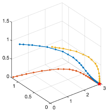
Figure 12: Trajectories of the GLV model with three initial conditions closely positioned to the other three semi-feasible equilibrium points. The globally sector stable semi-feasible equilibrium point is marked by the red star.

The feasibility requirement for equilibrium points in complex ecological models such as the GLV model drastically restricts their parameter space, especially when assuming random interactions. Consequently, most equilibrium points are semi-feasible, which highlights the importance and necessity of sector stability. Furthermore, Goh’s results indicate that a semi-feasible equilibrium point will likely be globally sector stable if the strength of self-regulating interactions surpasses that of interspecific interactions [106].

9 Structural stability analysis

The notion of structural stability of dynamical systems was first introduced by Andronov and Pontryagin under the name coarse (or rough) systems [17]. Different from the previous notions of stability which consider perturbations of initial conditions for a fixed dynamical system, structural stability concerns whether the qualitative behavior of the system trajectories will be affected by small perturbations of the system model itself [41, 192, 234, 252, 281]. In this section, we first discuss the mathematical definition of structural stability in dynamical systems. Then, we present various metrics that can be used to quantify the structural stability of ecological systems.

9.1 Mathematical definition

To formally define structural stability, we introduce the concept of topologically equivalence of dynamical systems. Two dynamical systems are called topologically equivalent if there is a homeomorphism $h:\mathbb{R}^{S}\to\mathbb{R}^{S}$ mapping their phase portraits, preserving the direction of time. Consider two smooth continuous-time dynamical systems (i) $\dot{\textbf{x}}(t)=\textbf{f}(\textbf{x}(t))$ and (ii) $\dot{\textbf{x}}(t)=\textbf{g}(\textbf{x}(t))$. Both systems (i) and (ii) are defined in a closed region $D\in\mathbb{R}^{S}$, see Figure 13a. System (i) is called structurally stable in a region $D_{0}\subset D$ if for any system (ii) that is sufficiently $C^{1}$-close to system (i) there are regions $U$, $V\subset D$, and $D_{0}\subset U$, $D_{0}\subset V$ such that system (i) is topologically equivalent in $U$ to system (ii) in $V$, see Figure 13a. Here, the systems (i) and (ii) are $C^{1}$-close if their “distance,” defined as

$$d=\sup_{\textbf{x}\in D}\left\{\|\textbf{f}(\textbf{x})-\textbf{g}(\textbf{x})\|+\left\|\frac{d\textbf{f}(\textbf{x})}{d\textbf{x}}-\frac{d\textbf{g}(\textbf{x})}{d\textbf{x}}\right\|\right\},$$

is small enough.

Andronov and Pontryagin offered sufficient and necessary conditions for a two-dimensional continuous-time dynamical system to be structurally stable [17]. A smooth dynamical system $\dot{\textbf{x}}(t)=\textbf{f}(\textbf{x}(t))$ with $\textbf{x}(t)\in\mathbb{R}^{2}$, is structurally stable in a region $D_{0}\subset\mathbb{R}^{2}$ if and only if (i) it has a finite number of equilibrium points and limit cycles in $D_{0}$, and all of them are hyperbolic; (ii) there are no saddle separatrices returning to the same saddle, see Figure 13b and c, or connecting two different saddles in $D_{0}$, see Figure 13d. This is often called the Andronov-Pontryagin criterion, which gives the complete description of structurally stable systems on the plane. It has been proven that a typical or generic two-dimensional system always satisfies the Andronov-Pontryagin criterion and hence is structurally stable [193]. In other words, structural stability is a generic property for planar systems. Yet, this is not true for high-dimensional systems. Later on, Morse and Smale established the sufficient conditions for an $S$-dimensional dynamical systems to be structurally stable [239, 240]. Such systems, often called Morse-Smale systems, have only a finite number of equilibrium points and limit cycles, all of which are hyperbolic and satisfy a transversaility condition on their stable and unstable invariant manifolds.

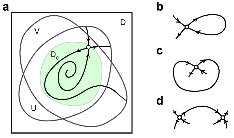
Figure 13: Structural stability. (a) Andronov’s definition of structural stability. (b-d) Phase portraits of structurally unstable planar systems. This figure was redrawn from [150].

9.2 Structural stability metrics

The notion of structural stability has been explored in diverse ecological systems. For instance, Recknagel investigated the structural stability of aquatic ecological systems by using the catastrophe theory and applied his approach as an aid in decision-making for water quality management [211]. In addition, the concept of structural stability have been heavily used in soil ecological systems [97, 194, 195, 225, 260]. Below, we survey various measures that can be used to quantify the structural stability of ecological systems.

Rohr et al. introduced a mathematical framework based on the concept of structural stability to elucidate the influence of network architecture on community persistence with the GLV model [215]. They proposed that an ecological system becomes more structurally stable as the area of the parameter space of the model expands, resulting in both a dynamically stable and feasible equilibrium. In particular, the authors investigated the range of conditions necessary for the stable coexistence of all species in mutualistic systems and showed that numerous observed mutualistic network architectures tend to maximize the volume of parameter space under which species coexist. This implies that having both a nested network architecture and a small mutualistic trade-off is one of the most preferable structures for community persistence.

Grilli et al. developed a geometrical framework to study the range of conditions necessary for feasible coexistence of large ecological systems [112]. They quantified the structural stability of an ecological system using the GLV model as the volume of the feasibility region when varying intrinsic growth rates, which can be approximated by

$$\Theta\approx\Bigg{(}1+\frac{1}{\pi}\frac{C_{A}\mu_{A}(2\mu_{d}-SC\mu_{A})}{\mu_{d}-SC^{2}\mu_{A}^{2}}\Bigg{)}^{S},$$ (28)

where $C_{A}$ is the connectance of the interaction matrix A, $\mu_{A}$ is the mean of the off-diagonal elements of A, and $\mu_{d}$ is the mean of the diagonal elements of A. The authors further analytically predicted the range of coexistence conditions in more than 100 empirical ecological systems. Recently, using the above approximation of structural stability, Portillo et al. explored the correlation between structural stability and various network measures, such as centrality and modularity, and illustrated that optimal modularity has a negative impact on biological diversity (structural stability) in empirical ecological systems [207].

During the same time, Saavedra et al. proposed novel metrics analogous to stabilizing niche differences and fitness differences with the GLV model, which can measure the range of conditions compatible with multi-species coexistence, i.e., structural stability [220]. The structural analogs of the niche and fitness differences are defined as

$$\Omega(\textbf{A})=\frac{|\text{det}(\textbf{A})|}{\sqrt[S]{\pi/2}}\int\cdots\int_{\mathbb{R}^{S}_{\geq 0}}e^{-\textbf{x}^{\top}\textbf{A}^{\top}\textbf{A}\textbf{x}}d\textbf{x}\quad\text{and}\quad\vartheta=\text{arccos}\Big{(}\frac{\textbf{r}^{\top}\textbf{r}_{c}}{\|\textbf{r}\|\|\textbf{r}_{c}\|}\Big{)},$$ (29)

respectively, where A is the interaction matrix, r is the vector of growth rates, and $\textbf{r}_{c}$ is the centroid of the feasibility domain defined as

$$\textbf{r}_{c}=\frac{1}{S}\Big{(}\frac{\textbf{a}_{1}}{\|\textbf{a}_{1}\|}+\frac{\textbf{a}_{2}}{\|\textbf{a}_{2}\|}+\cdots+\frac{\textbf{a}_{S}}{\|\textbf{a}_{S}\|}\Big{)}.$$

Here, $\textbf{a}_{i}$ denotes the $i$th column of A. Therefore, feasible solutions can be fulfilled as long as r is inside the cone defining the domain of feasibility $D(\textbf{A})=\{\textbf{r}\in\mathbb{R}^{S}_{>0}\text{ such that }\textbf{A}^{-1}\textbf{r}>0\}$. In other words, the structural analog of the fitness difference $\theta$ is small enough relative to the structural analog of the niche difference $\Omega(\textbf{A})$. The authors further applied their structural approach to a field system of annual plant competitors occurring on serpentine soils.

Saavedra and his coauthors have utilized similar approaches to study the structural stability of various ecological systems [60, 61, 216, 221, 222, 223, 242, 243, 244]. For example, they quantified structural stability using the quantity

$$\eta=\frac{(1-\cos^{2}{(\vartheta)}}{\cos^{2}{(\vartheta)}},$$ (30)

which measures how big the deviations are from the structural vector (geometric centroid) compatible with a positive stable equilibrium [222]. They further proved that the smaller the level of global competition, the broader the conditions for having feasible solutions. In addition, Song and Saavedra proposed a measure of structural stability using the quantity $\Omega(\textbf{A})^{1/S}$ with a transformation $2\textbf{A}^{\top}\textbf{A}=\boldsymbol{\Sigma}^{-1}$, which offers an approximation to the level of external perturbations tolerated by an ecological system [244]. The authors further found that their measure is the only consistent predictor of changes in species richness in empirical ecological systems among different ecological and environmental variables.

Lately, Pettersson et al. developed a metric called instability to quantify the proximity to collapse and level of structural stability with the GLV model, which provides deep insights into the dynamics and limits of stability and collapse of ecological systems [198]. The instability metric is defined as

$$\gamma(s)=\frac{\sigma_{A}-\sigma_{f}\big{(}S_{\text{pred}}(s)\big{)}}{\sigma_{c}\big{(}S_{\text{pred}}(s)\big{)}-\sigma_{f}\big{(}S_{\text{pred}}(s)\big{)}},$$ (31)

where $\sigma_{A}$ is the standard derivation of interspecific interaction strengths, $\sigma_{f}$ is the first extinction boundary, and $\sigma_{c}$ is the collapse boundary. Here, $S_{\text{pred}}(s)$ is the predicted initial biodiversity in terms of the actual biodiversity $s$. The metric $\gamma\in[0,1]$, and it can be computed from observable quantities of an ecological system. Notably, a higher $\gamma$ value indicates lower structural stability of a system, which increases the likelihood of collapse due to perturbations or external pressures.

10 Higher-order stability analysis

Various complex networks, such as ecological networks, social networks, biological networks, and chemical reaction networks, exhibit higher-order interactions, in which the interactions go beyond pairwise relationships and involve multiple nodes or entities at the same time [14, 40, 52, 54, 64, 63, 83, 99, 266]. In particular, in ecological networks, species interactions frequently occur in higher-order combinations, where the relationship between two species is influenced by one or more additional species [27, 143, 154], see Figure 14. From the modeling perspective, higher-order interactions can be explicitly modeled by adding higher-order terms to the classical GLV model. Alternatively, they can be implicitly captured through consumer-resource models, i.e., consumer species associated with the same resource form a higher-order interaction. While the significance of higher-order interactions has been recognized, their comprehensive impact on the stability of ecological systems has not been fully understood.

Pioneering research has shown that one type of third-order interaction, in which one species mitigates the negative interactions between two others, can stabilize well-mixed ecological systems with particular network configurations [139]. In addition, increasing the order of interactions among species can weaken the destabilizing effect and amplify the variance of species abundances at the equilibrium [78, 278]. In this section, we first introduce the GLV model with higher-order interactions and present various results related to the stability of ecological systems with higher-order interactions. We subsequently outline two potential approaches for analytically determining the stability of the GLV model with higher-order interactions via polynomial systems theory. Finally, we discuss various consumer-resource model for implicit higher-order interactions and their stability properties. Note that some results for higher-order stability also involve linear stability analysis.

10.1 GLV model with higher-order interactions

The dynamics of ecological systems with higher-order interactions are often described by the GLV model with higher-order interactions [6, 236] defined as

$$\begin{split}\dot{x}_{i}(t)&=x_{i}(t)\Big{[}r_{i}+\sum_{j=1}^{S}\textbf{A}_{ij}x_{j}(t)+\sum_{j=1}^{S}\sum_{k=1}^{S}\textsf{B}_{ijk}x_{j}(t)x_{k}(t)\\ &+\sum_{j=1}^{S}\sum_{k=1}^{S}\sum_{l=1}^{S}\textsf{C}_{ijkl}x_{j}(t)x_{k}(t)x_{l}(t)+\cdots\Big{]}\end{split}$$ (32)

for $i=1,2,\dots,S$. Here, $\textsf{B}\in\mathbb{R}^{S\times S\times S}$ is a third-order tensor whose off-diagonal elements represent the effect that species $j$ and $k$ has upon species $i$. $\textsf{C}\in\mathbb{R}^{S\times S\times S\times S}$ is a fourth-order tensor whose off-diagonal elements represent the effect that species $j$, $k$, $l$ has upon species $i$. In fact, the GLV model with higher-order interactions (32) belongs to the family of polynomial dynamical systems [62]. AlAdwani and Saavedra [6] determined the number of non-trivial equilibrium points of the GLV model with higher-order interactions (32) based on Bernshtein’s theorem [48] from algebraic geometry. However, the stability of those non-trivial equilibrium points remains unknown. So far, most of the stability analysis of higher-order interactions depends on linearization or numerical simulations of the GLV model with higher-order interactions or other similar models.

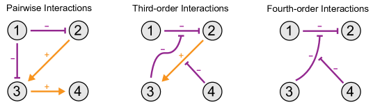
Figure 14: Examples of pairwise, third-order, and fourth-order interactions in ecological systems. For pairwise interactions, species 1 could produce an antibiotic, inhibiting the growth of species 2. For third-order interactions, species 3 might degrade the antibiotics produced by species 1, thus alleviating the inhibitory effect of species 1 on species 2. For fourth-order interactions, the activity of the antibiotic-degrading enzyme by species 3 may in turn be inhibited by compounds produced by species 4. This figure was redrawn from [27].

Bairey et al. found that the classical relationship between diversity and stability is reversed when considering high-order interactions by simulating the dynamics of ecological systems using a replicator model [27], which is defined based on the higher-order GLV model, with random interactions. Denote the bracket part in the GLV model with higher-order interactions (32) as $f_{i}(\textbf{x})$. The replicator model is defined as

$$\dot{x}_{i}(t)=x_{i}(t)\Big{[}f_{i}(\textbf{x})-\sum_{j=1}^{S}x_{j}f_{j}(\textbf{x})\Big{]},$$ (33)

where the extra term ensures x to be solved in the form of relative abundances. The authors further derived a stability criterion by examining the effective pairwise interactions through linearizing the higher-order interactions around an equilibrium point: an ecological system is stable with high probability if

$$\alpha+\frac{\beta}{S}+\frac{\gamma}{S^{2}}+\cdots<\frac{1}{S},$$ (34)

where $\alpha$, $\beta$, and $\gamma$ determines the strength (variance) of the pairwise, third-order, and fourth-order interactions, respectively. Therefore, interactions of any given order destabilize systems, and the impacts of different orders are additive, scaling differently with diversity. The combination of these interactions establishes both a lower and an upper bound on the number of species, which can be computed as

$$S_{\text{min,max}}=\frac{1-\beta\pm\sqrt{(1-\beta)^{2}-4\alpha\gamma}}{2\alpha}.$$

When the discriminant vanishes, i.e., $1-\beta=2\sqrt{\alpha\gamma}$, the two bounds narrow a defined optimal number of species $S^{*}=\sqrt{\gamma/\alpha}$.

Later on, Grilli et al. explored the role of higher-order interactions in competitive ecological systems [113]. Particularly, the authors simulated different competitive ecological systems with only third-order interactions of the form:

$$\dot{x_{i}}(t)=x_{i}(t)\Big{[}\sum_{j=1}^{S}\sum_{k=1}^{S}\textsf{B}_{ijk}x_{j}(t)x_{k}(t)\Big{]}$$ (35)

for $i=1,2,\dots,S$, which can be viewed as a special case of the higher-order GLV model. The interaction tensor B is defined from pairwise interactions and can be computed as $\textsf{B}_{ijk}=2\textbf{H}_{ij}\textbf{H}_{ik}-\textbf{H}_{ji}\textbf{H}_{jk}-\textbf{H}_{ki}\textbf{H}_{kj}$ where the first term represents the probability of species $i$ beats both species $j$ and $k$, and the remaining two terms represent the probabilities that either species $j$ or $k$ dominate. Here, the matrix H encodes the dominance relationships among species, i.e., $\textbf{H}_{ij}$ represents the probability that species $i$ outcompetes species $j$. Compared to the pairwise dynamics, the equilibrium point of (35) is unchanged, and more importantly, it is globally stable. Therefore, they concluded that incorporating higher-order interactions into competitive ecological systems enhances stability, making species coexistence resilient to perturbations of both population abundance and parameter values [113].

Singh and Baruah derived general rules for species coexistence modulated by higher-order interactions by simulating the higher-order GLV model [236]. They demonstrated that negative higher-order interactions can promote coexistence if these interactions strengthen intraspecific competition more than interspecific competition, while positive higher-order interactions can stabilize coexistence across a wide range of fitness differences, disregarding differences in strength of interspecific and intraspecific competition. Recently, Gibbs et al. also exploited the higher-order GLV model and found that when interspecific higher-order interactions became excessively harmful compared to self-regulation, the stability of coexistence in diverse ecological systems will be compromised [101]. Furthermore, they found that coexistence can also be lost when these interactions are weak and mutualistic higher-order effects became dominant [101].

10.2 Two potential approaches

As mentioned, the GLV model with higher-order interactions (32) belongs to the family of polynomial dynamical systems. Thus, polynomial systems theory can be leveraged to analytically study the stability properties of the model. We summarize two recent approaches that can analytically determine the stability of homogeneous polynomial dynamical systems [3, 62]. For simplicity, let’s assume that a higher-order ecological system with $S$ species only contains $p$th-order interactions. The resulting GLV model with higher-order interactions thus becomes homogeneous (of degree $p$), similar to the form (35). In fact, every polynomial dynamical system can be homogenized by introducing additional variables. Therefore, the two approaches can be in principle applied to analyze the stability of the GLV model with higher-order interactions.

10.2.1 Lyapunov approach

Ali and Khadir proved that the existence of a rational Lyapunov function, defined as the ratio of two polynomials, is both necessary and sufficient for asymptotic stability of a homogeneous polynomial dynamical system at the origin [3]. The rational Lyapunov function takes the form of

$$V(\textbf{x})=\frac{q(\textbf{x})}{(\sum_{i=1}^{S}x_{i}^{2})^{r}},$$

where $r$ is a non-negative integer and $q(\textbf{x})$ is a homogeneous positive definite polynomial of degree $2r+2$. Since the Lyapunov inequalities on both the rational function and its derivative have sum of squares certificates, $V(\textbf{x})$ can always be found by semi-definite programming [261].

The authors further proved that an $S$-dimensional homogeneous polynomial dynamical system of degree $p$ is asymptotically stable (in the sense of Lyapunov) at the origin if and only if there exist a non-negative integer $r$, a positive even integer $s$, with $2r<s$, and symmetric matrices $\textbf{P}\succeq\textbf{I}$ and $\textbf{Q}\succeq\textbf{I}$, such that

$$\big{\langle}\textbf{z}(\textbf{x}),\textbf{Q}\textbf{z}(\textbf{x})\big{\rangle}=-2\|\textbf{x}\|^{2}\big{\langle}J(\textbf{m}(\textbf{x}))^{\top}\textbf{P}\textbf{m}(\textbf{x}),\textbf{f}(\textbf{x})\big{\rangle}+2r\textbf{m}(\textbf{x})^{\top}\textbf{P}\textbf{m}(\textbf{x})\big{\langle}\textbf{x},\textbf{f}(\textbf{x})\big{\rangle},$$

where $\textbf{m}(\textbf{x})$ and $\textbf{z}(\textbf{x})$ denotes the vector of monomials in x of degree $\frac{s}{2}$ and $\frac{s+k+1}{2}$, respectively, and $J(\textbf{m}(\textbf{x}))$ denotes the Jacobian matrix of $\textbf{m}(\textbf{x})$ [3]. However, solving this hierarchy of semi-definite programs requires trying all possible combinations of $s$ and $r$, and the degree $s$ cannot be bounded solely based on the values of $S$ and $p$.

10.2.2 Tensor decomposition approach

Chen exploited tensor algebra to determine the stability of homogeneous polynomial dynamical systems [62]. First, the author proved that every $S$-dimensional homogeneous polynomial dynamical system of degree $p$ can be equivalently represented by a $(p+1)$th-order $S$-dimensional tensor, denoted by $\textsf{A}\in\mathbb{R}^{S\times S\times\stackrel{{\scriptstyle p+1}}{{\cdots}}\times S}$. Suppose that A is orthogonally decomposable, i.e.,

$$\textsf{A}=\sum_{i=1}^{S}\lambda_{i}\textbf{v}_{i}\circ\textbf{v}_{i}\circ\stackrel{{\scriptstyle p+1}}{{\cdots}}\circ\textbf{v}_{i},$$ (36)

where $\lambda_{i}$ are often referred to as the Z-eigenvalues of A with the corresponding Z-eigenvectors $\textbf{v}_{i}$ [214]. The stability properties of the homogeneous polynomial dynamical system can be readily obtained through the Z-eigenvalues, similar to linear stability. Let the initial condition $\textbf{x}_{0}=\sum_{i=1}^{S}\alpha_{i}\textbf{v}_{i}$. The equilibrium point $\textbf{x}^{*}=\textbf{0}$ is (i) stable if and only if $\lambda_{i}\alpha_{i}^{p-1}\leq 0$ for all $i$; (ii) asymptotically stable if and only if $\lambda_{i}\alpha_{i}^{p-1}<0$ for all $i$; (iii) unstable if and only if $\lambda_{i}\alpha_{i}^{p-1}>0$ for some $i$. When $p$ is odd, the initial condition can be ignored, and the stability conditions only depends on the Z-eigenvalues (exactly same as the case of linear stability).

The tensor decomposition approach provides straightforward criteria for determining the stability of homogeneous polynomial dynamical systems compared to the Lyapunov approach. Notably, Chen successfully employed this approach to analytically determine the stability of an ecological system described by the GLV model with higher-order interactions (considering third-order interactions only) with supply rates [62]. The model is defined as

$$\dot{x}_{i}(t)=x_{i}(t)\Big{[}\sum_{j=1}^{S}\sum_{k=1}^{S}\textsf{B}_{ijk}x_{j}(t)x_{k}(t)\Big{]}+s_{i},$$ (37)

where $s_{i}$ is the supply rate for species $i$. The stability of the model can be obtained for orthogonal decomposable B. However, not all tensors can be decomposed in the form of (36), which limits the applicability of this approach [214]. Nevertheless, we believe that both approaches (the Lyapunov and tensor decomposition approaches) have a significant potential for analytically understanding the stability of higher-order dynamics in ecological systems.

10.3 Implicit higher-order interactions

Implicit higher-order interactions have been considered in consumer-resource models [151]. MacArthur’s consumer-resource model is one of the most commonly used models for studying consumer-resource interactions [1, 70]. It is defined as

$$\begin{cases}\dot{x}_{i}(t)&=x_{i}(t)\Big{[}\theta_{i}\sum_{\alpha=1}^{N}\textbf{C}_{\alpha i}y_{\alpha}(t)-\mu_{i}\Big{]}\\ \dot{y}_{\beta}(t)&=y_{\beta}(t)\Big{[}\rho_{\beta}(1-\frac{y_{\beta}(t)}{K_{\beta}})-\sum_{j=1}^{S}\textbf{C}_{\beta j}x_{j}(t)\Big{]}\end{cases}$$ (38)

for $i=1,2,\dots,S$ and $\beta=1,2,\dots,N$, where $x_{i}(t)$ is the abundance of species $i$, $y_{\beta}$ is the abundance of resource $\beta$, $\theta_{i}\geq 0$ is the efficiency rate of species $i$ for converting the consumed resources into biomass, $\textbf{C}_{\alpha i}$ is the rate at which species $i$ consumers resource $\alpha$, $\mu_{i}$ is the mortality rate for species $i$, and $\rho_{\beta}$ and $K_{\beta}$ are the maximal growth rate and carrying capacity of resource $\beta$, respectively.

In MacArthur’s original formulation where the consumers and resources have different timescales, it can be shown that a feasible equilibrium point implies global stability by using a minimization principle [18, 25, 26]. Later on, the global asymptotic stability of MacArthur’s consumer-resource model with consumers and resources evolved in the same timescale has been proved by Case and Casten [59]. Notably, they rewrote MacArthur’s consumer-resource model into the GLV form (10) with

$$\footnotesize\tilde{\textbf{x}}=\begin{bmatrix}x_{1}\\ \vdots\\ x_{S}\\ y_{1}\\ \vdots\\ y_{N}\end{bmatrix},\text{ }\tilde{\textbf{r}}=\begin{bmatrix}-\mu_{1}\\ \vdots\\ -\mu_{S}\\ \rho_{1}\\ \vdots\\ \rho_{N}\end{bmatrix},\text{ }\tilde{\textbf{A}}=\begin{bmatrix}0&\cdots&0&\theta_{1}\textbf{C}_{11}&\cdots&\theta_{1}\textbf{C}_{N1}\\ \vdots&\vdots&\vdots&\vdots&\vdots&\vdots\\ 0&\cdots&0&\theta_{S}\textbf{C}_{1S}&\cdots&\theta_{S}\textbf{C}_{NS}\\ -\textbf{C}_{11}&\cdots&-\textbf{C}_{1S}&-\rho_{1}/K_{1}&\cdots&0\\ \vdots&\vdots&\vdots&\vdots&\vdots&\vdots\\ -\textbf{C}_{N1}&\cdots&-\textbf{C}_{NS}&0&\cdots&-\rho_{N}/K_{N}\end{bmatrix},$$

where $\tilde{\textbf{x}}$, $\tilde{\textbf{r}}$, and $\tilde{\textbf{A}}$ are the composite vector (or matrix) of species abundances, intrinsic growth rates, and interactions, respectively. Based on the formulated GLV model, they successfully constructed a Lyapunov function to demonstrate that any feasible equilibrium point is globally asymptotically stable.

Aparicio et al. explored the feasibility domain of MacArthur’s consumer-resource model [18]. Based on Case and Casten’s result, the feasibility domain can be automatically treated as the stability domain in MacArthur’s consumer-resource model. Specifically, the authors utilized the structural stability metrics as defined in (29) to compute the feasibility domain. Their findings unveil that the feasibility of MacArthur’s consumer-resource model diminishes with the pool size of the consumers increases, but the expected fraction of feasible consumers rises in this scenario [18]. Conversely, if resources exhibit linear growth, an increase in the resource pool reduces the feasibility of the model and the expected fraction of feasible consumers. However, if the resources increase logistically, the trend is reversed.

In the following, we present several results on the stability of consumer-resource models with various structure.

10.3.1 Impacts of cascade structure

Cascade structure plays a critical role in the stability of ecological systems [230]. Schreiber investigated the global stability of consumer-resource cascades (serially arranged containers with a dynamic consumer population that receives a flow of resources from the preceding container) [229]. The cascade model is defined as (assuming the numbers of consumers and resources are the same)

$$\begin{cases}\dot{x}_{i}(t)&=x_{i}(t)\Big{[}\theta\big{(}x_{i}(t)\big{)}h(y_{i}(t)/x_{i}(t)^{b})-\mu\big{(}x_{i}(t)\big{)}\Big{]}\\ \dot{y}_{i}(t)&=\gamma\big{(}y_{i-1}(t)-y_{i}(t)\big{)}-x_{i}(t)h(y_{i}(t)/x_{i}(t)^{b})\end{cases}$$ (39)

for $i=1,2,\dots,S$, where $\theta$ is the assimilation efficiency of the consumer dependent on $x_{i}$, $\mu$ is the mortality rate of the consumer dependent on $x_{i}$, $\gamma$ is the flow rate, and $h(y_{i}/x_{i}^{b})$ is the functional response for $b\in[0,1]$ [23]. To ensure both biological realism and mathematical tractability, it is assumed that (i) $h:\mathbb{R}\rightarrow\mathbb{R}$ is $C^{1}$ with $h(0)=0$ and $h^{\prime}(x)>0$ for all $x\geq 0$; (ii) The limit $h_{\infty}=\lim_{x\rightarrow\infty}h(x)$ exists and is finite; (iii) $\lim_{x\rightarrow\infty}xh^{\prime}(x)=0$; (iv) $0<\theta\leq 1$ and $\mu>0$ for all $x_{i}\geq 0$; (v) $\theta^{\prime}(x_{i})\leq 0$ and $\mu^{\prime}(x_{i})\geq 0$ for all $x_{i}$; (vi) $\theta(0)h_{\infty}-\mu(0)>0$. Under these assumptions (i)-(vi), the author proved that there exists an equilibrium point of the model which is globally stable. Hence, the ratio-dependent functional response can lead to persistence of the consumer population in all containers [229].

10.3.2 Impacts of mutualistic interactions

Microbial species capable of both resource consumption and production have the potential for mutualistic interactions [75, 280]. Butler and O’Dwyer explored the stability of a consumer-resource model with mutualistic interactions by explicitly considering the resources that microbes both consume and produce [58]. Their model is defined as (assuming the numbers of consumers and resources are the same)

$$\begin{cases}\dot{x}_{i}(t)&=x_{i}(t)\Big{[}\theta\sum_{j=1}^{S}\textbf{C}_{ji}y_{i}(t)-\sum_{j=1}^{S}\textbf{P}_{ji}-\mu_{i}\Big{]}\\ \dot{y}_{i}(t)&=\rho_{i}-y_{i}(t)\sum_{j=1}^{S}\textbf{C}_{ij}x_{j}(t)+\sum_{j=1}^{S}\textbf{P}_{ij}x_{j}(t)\end{cases}$$ (40)

for $i=1,2,\dots,S$, where $\textbf{P}_{ij}$ is the rate of the production of resource $i$ by consumer $j$, and other notations defined similarly as those in MacArthur’s consumer-resource model. For simplicity, they assumed that $\textbf{C}=c\textbf{I}$ meaning each consumer specializes on a single resource. In addition, the equilibrium points for the consumers and resources are simplified as $x^{*}\textbf{1}$ and $y^{*}\textbf{1}$, where 1 is the all-one vector, achieved by tuning the influx and mortality rates. This setting corresponds to the most general case of purely mutualistic interspecific interactions. The authors proved that feasible equilibrium points of the model are locally stable if

$$\Big{(}\sum_{j\neq i}\textbf{P}_{ij}\Big{)}^{2}<\frac{cx^{*}}{\theta}\Big{(}cy^{*}-\textbf{P}_{ii}-\frac{cx^{*}}{4\theta}\Big{)}$$ (41)

for all $i=1,2,\dots,S$, see Figure 15. Consequently, if microbes consume resources without producing them, any feasible equilibrium point will be locally stable. Yet, in the presence of cross-feeding, stability is no longer assured, where it can be obtained only when mutualistic interactions are sufficiently weak or when all pairs of taxa reciprocate each other’s assistance.

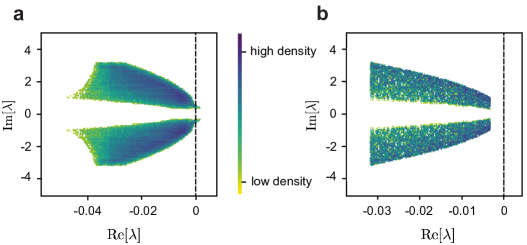
Figure 15: Eigenvalue distributions of the Jacobian matrix of the consumer-resource model with mutualistic interactions. (a) The randomly sampled production matrix P does not satisfy the condition (41), so there are positive eigenvalues. (b) The randomly sampled production matrix P satisfies the condition (41), so all eigenvalues are negative. This figure was drawn from [58].

10.3.3 Impacts of warming temperature

Temperature can affect the stability of ecological systems by causing changes in metabolic demands, ingestion rates, growth rates, and others [15, 16, 82, 102, 190]. Synodinos et al. used the classical Rosenzweig-MacArthur model [217] with a Holling type II functional response to study how temperature will alter stability [250]. The model is defined as (assuming one consumer and one resource)

$$\begin{cases}\dot{x}(t)&=x(t)\Big{[}\frac{\theta oy(t)}{1+oly(t)}-\mu\Big{]}\\ \dot{y}(t)&=y(t)\Big{[}\rho(1-\frac{y(t)}{K})-\frac{ox(t)}{1+oly(t)}\Big{]}\end{cases},$$ (42)

where $o$ is the consumer attack rate, $l$ is the handling time, $\mu$ is the mortality rate of the consumer, $\rho$ is the intrinsic growth rate of the resource, and $K$ is the carrying capacity of the resource. They analyzed the impacts of temperature on stability using the tendency for intrinsic oscillations in population abundances, which can be defined as $\varphi=olK$, i.e., the product of the three temperature-dependent parameters. The larger $\varphi$, the lower the stability of the ecological system. The authors found four different warming-stability patterns from various empirical ecological systems: stability increases, decreases, is hump-shaped or U-shaped with temperature.

10.3.4 Impacts of dynamic switching

The switching of the distribution of the rates of consumption between two resources is common in nature [145, 146, 147]. Gawronski et al. introduced a dynamic switching mechanism in the classical Rosenzweig-MacArthur consumer-resource model with one consumer and two resources [98]. The model is formulated as

$$\begin{cases}\dot{x}(t)&=x(t)\Big{[}o\frac{\theta_{1}y_{1}(t)+\theta_{2}y_{2}(t)}{1+l\big{(}\theta_{1}y_{1}(t)+\theta_{2}y_{2}(t)\big{)}}-\mu\Big{]}\\ \dot{y}_{1}(t)&=y_{1}(t)\Big{[}\big{(}1-\textbf{L}_{11}y_{1}(t)-\textbf{L}_{12}y_{2}(t)\big{)}-\frac{o\theta_{1}x(t)}{1+l\big{(}\theta_{1}y_{1}(t)+\theta_{2}y_{2}(t)\big{)}}\Big{]}\\ \dot{y}_{2}(t)&=y_{2}(t)\Big{[}\big{(}1-\textbf{L}_{21}y_{1}(t)-\textbf{L}_{22}y_{2}(t)\big{)}-\frac{o\theta_{2}x(t)}{1+l\big{(}\theta_{1}y_{1}(t)+\theta_{2}y_{2}(t)\big{)}}\Big{]}\end{cases},$$ (43)

where $\textbf{L}_{ij}$ represents the limitation of growth of resource $y_{i}$ imposed by resource $y_{j}$. The dynamic switching is driven by maximizing the consumer’s population $x$, i.e., $\dot{\theta}_{1}=(1/\tau)dx/d\theta_{1},$ where $\tau$ is the characteristic time. Through numerical simulations, the authors found that oscillations of the consumer and the mutually synchronized two resources, which emerge at $\theta_{i}=0.5$, become unstable for large or small $\theta_{i}$. Additionally, the model converges to a stable equilibrium point when either $\theta_{1}>0.5$ and $y_{1}<y_{2}$ or the opposite. This suggests that the consumer is unable to switch its preferred resource once it has been chosen.

10.3.5 Impacts of periodic environments

Periodic fluctuations and signals are widespread and strongly influence the structure and function of ecological systems [47, 219]. Bieg et al. investigated the role of periodic environmental forcing on consumer-resource interactions [51]. They used an extension of the classic Rosenzweig–MacArthur consumer-resource model [217] defined as (assuming one consumer and one resource)

$$\begin{cases}\dot{x}(t)&=x(t)\Big{[}\frac{\theta oy(t)}{\alpha+y(t)}-\mu\Big{]}\\ \dot{y}(t)&=y(t)\Big{[}\rho\big{(}1-\frac{y(t)}{K_{\text{mean}}+K_{\text{force}}(t)}\big{)}-\frac{ox(t)}{\alpha+y(t)}\Big{]}\end{cases},$$ (44)

where $\alpha$ is the half-saturation coefficient, $K_{\text{mean}}$ is the average resource carrying capacity, and $K_{\text{force}}(t)$ is a sinusoidal function capturing periodic forces defined as

$$K_{\text{force }}(t)=A\sin{(p2\pi t)}.$$

Here, $A$ is the amplitude of the forcing, and $p$ is the forcing speed. Through local stability analysis, the authors found that the forcing speed significantly affects the stability of the model, with fast environmental forcing having a stabilizing effect. Their results further suggest that periodic fluctuations from climate change may cause sudden shifts in ecological dynamics and stability.

10.3.6 Impacts of consumption threshold

The idea of consumption threshold is borrowed from the basic reproduction in epidemiological models [259]. Duffy and Collins introduced this notion to determine the stability of the classical Rosenzweig-MacArthur consumer-resource model [84], which is defined similarly as (assuming one consumer and one resource)

$$\begin{cases}\dot{x}(t)&=x(t)\Big{[}\frac{\theta oy(t)}{\alpha+y(t)}-\mu\Big{]}\\ \dot{y}(t)&=y(t)\Big{[}\rho(1-\frac{y(t)}{K})-\frac{ox(t)}{\alpha+y(t)}\Big{]}\end{cases}.$$ (45)

The consumption threshold is defined as $C_{0}=\frac{\theta oK}{\mu(\alpha+K)}$. Ecologically, it represents the parameter combination that guarantees the minimum resource consumption required for the consumer to survive. The authors proved that the trivial equilibrium point (i.e., $x^{*}=y^{*}=0$) is always unstable, and the semi-feasible equilibrium point (i.e., $x^{*}=0$ and $y^{*}=K$) is locally stable if $C_{0}\leq 1$. Furthermore, They also demonstrated that the model undergoes a Hopf bifurcation at

$$C_{0}^{*}=\frac{K}{\alpha+K}\Big{(}1+\frac{(\mu+\theta o)\alpha}{\mu K}\Big{)},$$

and the non-trivial equilibrium point (i.e., $x^{*}>0$ and $y^{*}>0$) exists for $C_{0}>1$ and is locally stable if $C_{0}<C_{0}^{*}$. In summary, when the consumption threshold $C_{0}\leq 1$, only the resource can survive, while when $C_{0}>1$, both the consumer and resource can coexist.

10.3.7 Impacts of delayed age structure

The introduction of delay in the consumer-resource models plays a significant role in their stability. Akimenko studied the stability of a delayed age-structural consumer-resource model with $N$ resource patches and consumers that can move freely between the patches [4]. The resource dynamics of the model is defined as

$$\dot{y}_{i}(t)=y_{i}(t)\Bigg{[}\rho_{i}\Big{(}1-\frac{y_{i}(t)}{K_{i}}\Big{)}-\frac{\beta_{i}\hat{X}(t)}{1+\alpha_{i}\hat{X}(t)}\Bigg{]}$$ (46)

for $i=1,2,\dots,N$, where $\beta_{i}>0$ is the search rate, $\alpha_{i}\geq 0$ is the saturation coefficient, and $\hat{X}(t)=\int_{0}^{a_{d}}\kappa(a)x(a,t)da$ is the weighted quantity of consumers at time $t$. Here, $\kappa(a)$ represents the age-specific consumer’s preference, and $x(a,t)$ is the age-specific density of consumer population at age $a$ and time $t$. On the other hand, the consumer dynamics $x(a,t)$ is described by the delayed McKendrick-Von Foerster’s age-structured model [93, 118, 119] defined as

$$\frac{\partial x}{\partial t}+\frac{\partial x}{\partial a}=-\mu\big{(}a,w(t-\tau)\big{)}x(a,t),$$ (47)

where $\mu(a,w)$ is the age- and calorie intake rate-dependent consumer mortality rate. Combined with initial and boundary conditions, the author proved that the trivial equilibrium point (i.e., $y_{i}^{*}=0$ and $x^{*}(a)=0$) of the model is unstable for all $\tau>0$ and the semi-feasible equilibrium point (i.e., $y_{i}^{*}=K_{i}$ and $x^{*}(a)=0$) is locally asymptotically stable if the consumer’s basic reproduction number $R(w^{*})<1$ and is unstable if $R(w^{*})\geq 1$ for all $\tau>0$. The consumer’s basic reproduction number dependent on the calorie intake rate $w$ is defined as

$$R(w)=\int_{a_{r}}^{a_{m}}\Omega(a,w)\exp{\Big{(}-\int_{0}^{a}\mu(\zeta,w)d\zeta\Big{)}da},$$

where $\Omega(a,w)$ is the age- and calorie intake rate-dependent consumer fertility rate, and $a_{r}$ and $a_{m}$ are the age of maturation and maximum age of reproduction, respectively. Furthermore, the non-trivial equilibrium point (i.e., $y_{i}^{*}>0$ for some $i$ and $x^{*}(a)>0$) exists if and only if $R(w^{*})=1$. Define $I_{0}=\{i\text{ }|\text{ }y^{*}_{i}=0\}$. The non-trivial equilibrium point is unstable for all $\tau>0$ if $I_{0}\neq\emptyset$ and at least one of the following conditions is satisfied: (i) there exists $i\in I_{0}$ such that $\alpha_{i}\geq\beta_{i}/\rho_{i}$; or (ii) $\alpha_{i}<\beta_{i}/\rho_{i}$ for all $i\in I_{0}$ and $\hat{X}^{*}\leq\max_{i\in I_{0}}(\beta_{i}/\rho_{i}-\alpha_{i})^{-1}$. It is locally asymptotically stable for all $\tau>0$ if one of the following conditions is satisfied: (iii) $I_{0}\neq\emptyset$, $\alpha_{i}<\beta_{i}/\rho_{i}$ for all $i\in I_{0}$, and $\hat{X}^{*}>\max_{i\in I_{0}}(\beta_{i}/\rho_{i}-\alpha_{i})^{-1}$; (iv) $I_{0}=\emptyset$. Akimenko’s findings show that the digestion period (i.e., the delay parameter) $\tau$ does not destabilize the consumer population at the trivial, semi-feasible or non-trivial equilibrium points.

Recently, El-Doma improved the stability criteria proposed by Akimenko in analyzing the delayed age-structural consumer-resource model (46) and (47) [87]. Notably, the author proved that the non-trivial equilibrium point (with $I_{0}\neq\emptyset$) of the model is locally asymptotically stable if $X^{*}(\beta_{i}/\rho_{i}-\alpha_{i})>1$ and is unstable if $X^{*}(\beta_{i}/\rho_{i}-\alpha_{i})<1$ for $i\in I_{0}$. Clearly, the conditions are simpler than Akimenko’s.

10.3.8 A case study of larch moth interactions

Plant’s quality plays an important role in the population dynamics of consumers [129, 130]. Din and Khan explored the dynamics between budmoths and the quality of larch trees located in the Swiss Alps [80]. They proposed an improved discrete-time consumer-resource model to capture the interactions between the plant quality index $x$ and the moth population density $y$ defined as

$$\begin{cases}x(t+1)&=(1-v)+vx(t)-\frac{uy(t)}{\alpha+y(t)}\\ y(t+1)&=y(t)\exp{\Big{(}\rho(\frac{x(t)}{\beta+x(t)}-\frac{y(t)}{K})\Big{)}}\end{cases},$$ (48)

where $0<v<1$ is the plant vulnerability, $u$ is the moth’s maximal uptake rate of the plant, $\alpha$ and $\beta$ are the half-saturation coefficients, $\rho$ is the growth rate of moths, and $K$ is the carrying capacity of moths. The authors proved that the model has a non-trivial equilibrium point, and it is locally asymptotically stable if and only if

$$\begin{split}\frac{\beta\alpha\rho uy^{*}}{(\beta+x^{*})^{2}(\alpha+y^{*})^{2}}+\frac{(v+1)(2K-\rho y^{*})}{K}&>0,\\ v+\frac{\beta\alpha\rho uy^{*}}{(\beta+x^{*})^{2}(\alpha+y^{*})^{2}}-\frac{v\rho y^{*}}{K}&<1.\end{split}$$ (49)

The model also undergoes a period-doubling bifurcation at the non-trivial equilibrium point. Significantly, Din and Khan validated their theoretical findings with experimental data.

11 Discussion

The seven stability notions we reviewed, including linear stability, sign stability, diagonal stability, D-stability, total stability, structural stability, and higher-order stability, are not mutually exclusive but rather complement each other, which offers a multifaceted approach to explore the stability of ecological systems. Next, we discuss the pros and cons of each stability notion and outline its potential future prospects.

Linear stability analysis is the most widely used approach to study the stability of ecological systems due to its simplicity. It has been heavily used in ecological systems with various network structures, as presented in Section 3. However, it cannot precisely capture the global dynamics and complex behaviors of ecological systems that are highly nonlinear in reality. Nevertheless, it will be interesting to perform the linear stability analysis on more complex models, such as the GLV model with higher-order interactions. For example, how to express the community matrix M in terms of the interaction matrix A and the higher-order interaction tensors, and how to establish stability conditions based on higher-order interaction strengths and correlations with various higher-order network structures?

Sign stability analysis focuses on the qualitative nature of interactions in ecological systems, disregarding of their magnitudes. It is particularly advantageous when quantitative data on interaction strengths are missing. However, the conditions described in Section 4 are too stringent to realize in real ecological systems. Hence, it will be intriguing to explore simpler and more realizable conditions that are associated to the underlying network structure for the sign stability of an ecological system. Generalizing the notion to nonlinear models, e.g., the GLV model or the GLV model with higher-order interactions, also presents exciting avenues for further work.

Diagonal stability, D-stability, and total stability analyses contribute to enhancing the understanding of the stability of the GLV model through characterizing the interaction matrix A. Moreover, they provide an insightful exploration of how the network structure encoded in the interaction matrix impact the overall stability of an ecological system. Nevertheless, characterizing diagonally stable, D-stable, or totally stable matrices is increasingly difficult for high-dimensional systems. Therefore, it will be worthwhile to further explore various network structures that can be used to establish necessary or sufficient conditions for achieving diagonally stability, D-stability, or total stability with the GLV model. Extending the current results to the GLV model with higher-order interactions also holds promising avenues for future research.

Sector stability analysis is particularly useful when dealing with semi-feasible equilibrium points, which are prevalent in modeling ecological systems. Local sector stability can be readily assessed, but a definitive algorithmic approach for verifying global sector stability remains elusive. For example, how can we efficiently compute the crucial constant matrix G defined in Section 8? Moreover, it will be worthwhile to explore simplified conditions on the sector stability of other nonlinear ecological models such as the GLV model with higher-order interactions and MacArthur’s consumer-resource model.

Structural stability analysis assesses how the overall behavior of an ecological system is maintained under small perturbations, which is different from all the previous stability notions. Structural stability can offer unique insights into the feasibility and robustness of ecological systems. An interesting avenue for future research would involve comparing various structural stability metrics and understanding their implications for the underlying network structure of an ecological system. Nonetheless, all the current structural stability metrics are developed based on the GLV model. Thus, extending these metrics to more complicated models, such as the GLV model with higher-order interactions, would also be a valuable exploration.

Higher-order stability analysis recently becomes popular due to the importance of higher-order interactions in ecological systems. It takes into account the nonlinearity inherent in ecological systems, providing more accurate representations, e.g., the GLV model with higher-order interactions. Yet, the stability analysis of such higher-order models is challenging. As interactions become more complex, involving multiple species simultaneously, the mathematical complexity of the analysis increases significantly. As mentioned in Section 10, the Lyapunov and tensor decomposition approaches are promising for investigating the stability of the GLV model with higher-order interactions, which often possesses multiple feasible equilibrium points.

12 Conclusion

In this article, we presented a comprehensive and systematic review of the literature concerning the stability of ecological systems. Notably, we inclusively surveyed various stability notions that arise in ecological systems, encompassing linear stability, sign stability, diagonal stability, D-stability, total stability, sector stability, structural stability, and higher-order stability.

As mentioned earlier, empirically applying this theory to real ecological systems poses a significant challenge. First, most of the stability criteria are derived from the random matrix theory, which cannot accurately capture real ecological systems. For instance, the food web topology studies have demonstrated the non-randomness of ecological systems, rendering to incorporate more realistic network structures [152]. Second, the dynamics governing real ecological systems could not adhere to the GLV model, or even unknown in many cases. Thus, the stability analysis of real ecological systems may not align with the predictions of the theory.

Table 4: Summary of the most commonly used databases for real ecological systems. Links to the databases are provided.

Database	Description	References
Web of Life	A graphical user interface for visualizing and downloading data on plant-animal mutualistic ecological networks.	[94]
Network Repository	A network repository containing hundreds of real-world networks including ecological networks.	[218]
GloBI	An extensible and open-source infrastructure for importing, searching, and exporting species-interaction data.	[204]
NEON	Monitoring ecological systems, including freshwater and terrestrial systems across the United States.	[175, 176]
Global Web	An online collection of food webs.	N/A
DoPI	Comprising ecological networks of British pollinator-plant interactions from the published scientific literature or submitted datasets.	[28, 110, 185]

Additionally, applying those various stability analysis to empirical ecological systems requires accurate estimation of the species interaction matrix or community matrix. For example, the trophic flows between consumers and resources in a food web with eco-path model can be translated into the interaction coefficients of the GLV model [128]. However, inferring the interaction network for large ecological systems, e.g., microbial communities, is challenging. Alternative frameworks, such as sensitivity testing of species abundance in response to the presence of additional species [277], may prove valuable for assessing the connectance and interaction strength of the interaction matrix or community matrix. To facilitate research in this field, we have compiled a summary of the most commonly used databases for real ecological systems in Table 4.

Finally, these stability analyses could be applied to other systems beyond ecological systems, such as power grid and gene regulatory networks. For example, the stability of power-grid networks in the homogeneous state, where the voltage frequencies of generators are all equal to a constant reference frequency, requires the largest eigenvalues of the Jacobian matrix to be negative [172]. Similarly, the stability of gene regulatory networks in regimes where the lifetime of mRNAs is much shorter than that of proteins depends solely on the eigenvalues of the Jacobian matrix. Furthermore, in the case of random gene regulatory networks, the underlying system becomes unstable when either the system size exceeds a critical threshold or the regulation strength becomes too strong, as determined using random matrix theory, which aligns with May’s theory [69].

Declaration of Generative AI and AI-assisted technologies in the writing process

During the preparation of this work, the authors used ChatGPT in order to improve readability and language. After using this tool, the authors reviewed and edited the content as needed and take full responsibility for the content of the publication.

References

- [1] Madhu Advani, Guy Bunin, and Pankaj Mehta. Statistical physics of community ecology: a cavity solution to macarthur’s consumer resource model. Journal of Statistical Mechanics: Theory and Experiment, 2018(3):033406, 2018.
- [2] HN Agiza, EM Elabbasy, H El-Metwally, and AA Elsadany. Chaotic dynamics of a discrete prey–predator model with holling type ii. Nonlinear analysis: Real world applications, 10(1):116–129, 2009.
- [3] Amir Ali Ahmadi and Bachir El Khadir. On algebraic proofs of stability for homogeneous vector fields. IEEE Transactions on Automatic Control, 65(1):325–332, 2019.
- [4] Vitalii V Akimenko. Stability analysis of delayed age-structured resource-consumer model of population dynamics with saturated intake rate. Frontiers in Ecology and Evolution, 9:531833, 2021.
- [5] Jafar Fawzi M Al-Omari and Stephen A Gourley. Stability and traveling fronts in lotka-volterra competition models with stage structure. SIAM Journal on Applied Mathematics, 63(6):2063–2086, 2003.
- [6] Mohammad AlAdwani and Serguei Saavedra. Is the addition of higher-order interactions in ecological models increasing the understanding of ecological dynamics? Mathematical Biosciences, 315:108222, 2019.
- [7] Mohammad AlAdwani and Serguei Saavedra. Ecological models: higher complexity in, higher feasibility out. Journal of The Royal Society Interface, 17(172):20200607, 2020.
- [8] Alexander Aleksandrov and Oliver Mason. Diagonal stability of a class of discrete-time positive switched systems with delay. IET Control Theory & Applications, 12(6):812–818, 2018.
- [9] S. Allesina and S. Tang. Stability criteria for complex ecosystems. Nature, 483:205–208, 2012.
- [10] Stefano Allesina, Jacopo Grilli, György Barabás, Si Tang, Johnatan Aljadeff, and Amos Maritan. Predicting the stability of large structured food webs. Nature communications, 6(1):7842, 2015.
- [11] Stefano Allesina and Mercedes Pascual. Network structure, predator–prey modules, and stability in large food webs. Theoretical Ecology, 1:55–64, 2008.
- [12] Stefano Allesina and Si Tang. The stability–complexity relationship at age 40: a random matrix perspective. Population Ecology, 57(1):63–75, 2015.
- [13] Ada Altieri, Felix Roy, Chiara Cammarota, and Giulio Biroli. Properties of equilibria and glassy phases of the random lotka-volterra model with demographic noise. Physical Review Letters, 126(25):258301, 2021.
- [14] Unai Alvarez-Rodriguez, Federico Battiston, Guilherme Ferraz de Arruda, Yamir Moreno, Matjaž Perc, and Vito Latora. Evolutionary dynamics of higher-order interactions in social networks. Nature Human Behaviour, 5(5):586–595, 2021.
- [15] Priyanga Amarasekare. Effects of temperature on consumer–resource interactions. Journal of Animal Ecology, 84(3):665–679, 2015.
- [16] Priyanga Amarasekare. Effects of climate warming on consumer-resource interactions: a latitudinal perspective. Frontiers in Ecology and Evolution, 7:146, 2019.
- [17] Aleksandr A. Andronov and Lev S. Pontryagin. Systémes grossiers. Doklady Akademii Nauk SSSR, 14(5):247–251, 1937.
- [18] Andrea Aparicio, Tong Wang, Serguei Saavedra, and Yang-Yu Liu. Feasibility in macarthur’s consumer-resource model. Theoretical Ecology, 2023.
- [19] Murat Arcak. Diagonal stability on cactus graphs and application to network stability analysis. IEEE Transactions on Automatic Control, 56(12):2766–2777, 2011.
- [20] Murat Arcak and Eduardo Sontag. A passivity-based stability criterion for a class of biochemical reaction networks. Mathematical biosciences and engineering, 5(1):1, 2008.
- [21] Murat Arcak and Eduardo D Sontag. Diagonal stability of a class of cyclic systems and its connection with the secant criterion. Automatica, 42(9):1531–1537, 2006.
- [22] Murat Arcak and Eduardo D. Sontag. A passivity-based stability criterion for a class of interconnected systems and applications to biochemical reaction networks. In 2007 46th IEEE Conference on Decision and Control, pages 4477–4482, 2007.
- [23] Roger Arditi, Nicolas Perrin, and Henni Saïah. Functional responses and heterogeneities: an experimental test with cladocerans. Oikos, pages 69–75, 1991.
- [24] Kenneth J Arrow and Maurice McManus. A note on dynamic stability. Econometrica: Journal of the Econometric Society, pages 448–454, 1958.
- [25] Robert Mac Arthur. Species packing, and what competition minimizes. Proceedings of the National Academy of Sciences, 64(4):1369–1371, 1969.
- [26] Robert Mac Arthur. Species packing and competitive equilibrium for many species. Theoretical population biology, 1(1):1–11, 1970.
- [27] Eyal Bairey, Eric D Kelsic, and Roy Kishony. High-order species interactions shape ecosystem diversity. Nature communications, 7(1):12285, 2016.
- [28] Nicholas J Balfour, Jeff Ollerton, Maria Clara Castellanos, and Francis LW Ratnieks. British phenological records indicate high diversity and extinction rates among late-summer-flying pollinators. Biological Conservation, 222:278–283, 2018.
- [29] CS Ballantine. Stabilization by a diagonal matrix. Proceedings of the American Mathematical Society, 25(4):728–734, 1970.
- [30] György Barabás, Matthew J Michalska-Smith, and Stefano Allesina. Self-regulation and the stability of large ecological networks. Nature ecology & evolution, 1(12):1870–1875, 2017.
- [31] Matthieu Barbier, Claire De Mazancourt, Michel Loreau, and Guy Bunin. Fingerprints of high-dimensional coexistence in complex ecosystems. Physical Review X, 11(1):011009, 2021.
- [32] Milton Barbosa, Geraldo Wilson Fernandes, and Rebecca Jane Morris. Experimental evidence for a hidden network of higher-order interactions in a diverse arthropod community. Current Biology, 33(2):381–388, 2023.
- [33] H Barclay and P van den Driesschei. Deterministic population models and stability. SIAM Review, 20(2):389–393, 1978.
- [34] George Phillip Barker, Abraham Berman, and Robert J Plemmons. Positive diagonal solutions to the lyapunov equations. Linear and Multilinear Algebra, 5(4):249–256, 1978.
- [35] Joseph W Baron. Eigenvalue spectra and stability of directed complex networks. Physical Review E, 106(6):064302, 2022.
- [36] Joseph W Baron and Tobias Galla. Dispersal-induced instability in complex ecosystems. Nature communications, 11(1):6032, 2020.
- [37] Joseph W Baron, Thomas Jun Jewell, Christopher Ryder, and Tobias Galla. Eigenvalues of random matrices with generalized correlations: A path integral approach. Physical Review Letters, 128(12):120601, 2022.
- [38] Joseph W Baron, Thomas Jun Jewell, Christopher Ryder, and Tobias Galla. Breakdown of random-matrix universality in persistent lotka-volterra communities. Physical Review Letters, 130(13):137401, 2023.
- [39] Jordi Bascompte. Structure and dynamics of ecological networks. Science, 329(5993):765–766, 2010.
- [40] Federico Battiston, Enrico Amico, Alain Barrat, Ginestra Bianconi, Guilherme Ferraz de Arruda, Benedetta Franceschiello, Iacopo Iacopini, Sonia Kéfi, Vito Latora, Yamir Moreno, et al. The physics of higher-order interactions in complex systems. Nature Physics, 17(10):1093–1098, 2021.
- [41] Zdeněk P Bažant. Structural stability. International Journal of Solids and Structures, 37(1-2):55–67, 2000.
- [42] E Beretta and F Solimano. A generalization of volterra models with continuous time delay in population dynamics: Boundedness and global asymptotic stability. SIAM Journal on Applied Mathematics, 48(3):607–626, 1988.
- [43] E Beretta and Y Takeuchi. Global asymptotic stability of lotka–volterra diffusion models with continuous time delay. SIAM Journal on Applied Mathematics, 48(3):627–651, 1988.
- [44] Claude Berge. Hypergraphs: combinatorics of finite sets, volume 45. Elsevier, 1984.
- [45] A Berman and R Plemmons. Nonnegative Matrices in the Mathematical Sciences. SIAM, 1994.
- [46] Abraham Berman and Daniel Hershkowitz. Matrix diagonal stability and its implications. SIAM Journal on Algebraic Discrete Methods, 4(3):377–382, 1983.
- [47] Joey R Bernhardt, Mary I O’Connor, Jennifer M Sunday, and Andrew Gonzalez. Life in fluctuating environments. Philosophical Transactions of the Royal Society B, 375(1814):20190454, 2020.
- [48] David N Bernshtein. The number of roots of a system of equations. Funktsional’nyi Analiz i Ego Prilozheniya, 9(3):1–4, 1975.
- [49] Subhash C Bhargava. Generalized lotka-volterra equations and the mechanism of technological substitution. Technological Forecasting and Social Change, 35(4):319–326, 1989.
- [50] Amit Bhaya and Eugenius Kaszkurewicz. On discrete-time diagonal and d-stability. Linear Algebra and its Applications, 187:87–104, 1993.
- [51] Carling Bieg, Gabriel Gellner, and Kevin S McCann. Stability of consumer–resource interactions in periodic environments. Proceedings of the Royal Society B, 290(2007):20231636, 2023.
- [52] Ian Billick and Ted J Case. Higher order interactions in ecological communities: what are they and how can they be detected? Ecology, 75(6):1529–1543, 1994.
- [53] Giulio Biroli, Guy Bunin, and Chiara Cammarota. Marginally stable equilibria in critical ecosystems. New Journal of Physics, 20(8):083051, 2018.
- [54] Stefano Boccaletti, Pietro De Lellis, CI del Genio, Karin Alfaro-Bittner, Regino Criado, Sarika Jalan, and Miguel Romance. The structure and dynamics of networks with higher order interactions. Physics Reports, 1018:1–64, 2023.
- [55] Stephen Boyd, Laurent El Ghaoui, Eric Feron, and Venkataramanan Balakrishnan. Linear Matrix Inequalities in System and Control Theory. SIAM, Philadelphia, 1994.
- [56] Brian Buma and Courtney Schultz. Disturbances as opportunities: Learning from disturbance-response parallels in social and ecological systems to better adapt to climate change. Journal of Applied Ecology, 57(6):1113–1123, 2020.
- [57] Guy Bunin. Ecological communities with lotka-volterra dynamics. Physical Review E, 95(4):042414, 2017.
- [58] Stacey Butler and James P O’Dwyer. Stability criteria for complex microbial communities. Nature communications, 9(1):2970, 2018.
- [59] Ted J Case and Richard G Casten. Global stability and multiple domains of attraction in ecological systems. The American Naturalist, 113(5):705–714, 1979.
- [60] Simone Cenci and Serguei Saavedra. Structural stability of nonlinear population dynamics. Physical Review E, 97(1):012401, 2018.
- [61] Simone Cenci, Chuliang Song, and Serguei Saavedra. Rethinking the importance of the structure of ecological networks under an environment-dependent framework. Ecology and evolution, 8(14):6852–6859, 2018.
- [62] Can Chen. Explicit solutions and stability properties of homogeneous polynomial dynamical systems. IEEE Transactions on Automatic Control, 68(8):4962–4969, 2023.
- [63] Can Chen, Chen Liao, and Yang-Yu Liu. Teasing out missing reactions in genome-scale metabolic networks through hypergraph learning. Nature Communications, 14(1):2375, 2023.
- [64] Can Chen and Yang-Yu Liu. A survey on hyperlink prediction. IEEE Transactions on Neural Networks and Learning Systems, 2023.
- [65] Can Chen and Indika Rajapakse. Tensor entropy for uniform hypergraphs. IEEE Transactions on Network Science and Engineering, 7(4):2889–2900, 2020.
- [66] Can Chen, Amit Surana, Anthony Bloch, and Indika Rajapakse. Multilinear time invariant system theory. In 2019 Proceedings of the Conference on Control and its Applications, pages 118–125. SIAM, 2019.
- [67] Can Chen, Amit Surana, Anthony M Bloch, and Indika Rajapakse. Controllability of hypergraphs. IEEE Transactions on Network Science and Engineering, 8(2):1646–1657, 2021.
- [68] Can Chen, Amit Surana, Anthony M Bloch, and Indika Rajapakse. Multilinear control systems theory. SIAM Journal on Control and Optimization, 59(1):749–776, 2021.
- [69] Luonan Chen and Kazuyuki Aihara. Stability of genetic regulatory networks with time delay. IEEE Transactions on circuits and systems I: Fundamental Theory and Applications, 49(5):602–608, 2002.
- [70] Peter Chesson. Macarthur’s consumer-resource model. Theoretical Population Biology, 37(1):26–38, 1990.
- [71] Villy Christensen and Daniel Pauly. Ecopath ii—a software for balancing steady-state ecosystem models and calculating network characteristics. Ecological modelling, 61(3-4):169–185, 1992.
- [72] Tianguang Chu. An equivalent condition for stability properties of lotka–volterra systems. Physics Letters A, 368(3-4):235–237, 2007.
- [73] Bruce L Clarke. Theorems on chemical network stability. The Journal of Chemical Physics, 62(3):773–775, 1975.
- [74] KL Cottingham, BL Brown, and JT Lennon. Biodiversity may regulate the temporal variability of ecological systems. Ecology Letters, 4(1):72–85, 2001.
- [75] Katharine Z Coyte, Jonas Schluter, and Kevin R Foster. The ecology of the microbiome: networks, competition, and stability. Science, 350(6261):663–666, 2015.
- [76] GW Cross. Three types of matrix stability. Linear algebra and its applications, 20(3):253–263, 1978.
- [77] Jeffrey M Dambacher, Hang-Kwang Luh, Hiram W Li, and Philippe A Rossignol. Qualitative stability and ambiguity in model ecosystems. The American Naturalist, 161(6):876–888, 2003.
- [78] Viviane M de Oliveira and JF Fontanari. Random replicators with high-order interactions. Physical review letters, 85(23):4984, 2000.
- [79] Peter C De Ruiter, Anje-Margriet Neutel, and John C Moore. Energetics, patterns of interaction strengths, and stability in real ecosystems. Science, 269(5228):1257–1260, 1995.
- [80] Qamar Din and Muhammad Irfan Khan. A discrete-time model for consumer–resource interaction with stability, bifurcation and chaos control. Qualitative theory of dynamical systems, 20(2):56, 2021.
- [81] Stephanie Domptail, Marcos H Easdale, and Yuerlita. Managing socio-ecological systems to achieve sustainability: A study of resilience and robustness. Environmental Policy and Governance, 23(1):30–45, 2013.
- [82] Ian Donohue, Helmut Hillebrand, José M Montoya, Owen L Petchey, Stuart L Pimm, Mike S Fowler, Kevin Healy, Andrew L Jackson, Miguel Lurgi, Deirdre McClean, et al. Navigating the complexity of ecological stability. Ecology letters, 19(9):1172–1185, 2016.
- [83] Gabrielle A Dotson, Can Chen, Stephen Lindsly, Anthony Cicalo, Sam Dilworth, Charles Ryan, Sivakumar Jeyarajan, Walter Meixner, Cooper Stansbury, Joshua Pickard, et al. Deciphering multi-way interactions in the human genome. Nature Communications, 13(1):5498, 2022.
- [84] Kevin Jan Duffy and Obiora Cornelius Collins. Identifying stability conditions and hopf bifurcations in a consumer resource model using a consumption threshold. Ecological Complexity, 28:212–217, 2016.
- [85] Denis Efimov and A Yu Aleksandrov. Robust stability analysis and implementation of persidskii systems. In 2019 IEEE 58th Conference on Decision and Control (CDC), pages 6164–6168. IEEE, 2019.
- [86] Denis Efimov and Alexander Aleksandrov. On analysis of persidskii systems and their implementations using lmis. Automatica, 134:109905, 2021.
- [87] M El-Doma. An age-structured consumer-resource model with delay i: Steady states and preliminary stability results. Journal of Applied Mathematics and Computation, 7(1):19–23, 2023.
- [88] Clive Emary and Darren Evans. Can a complex ecosystem survive the loss of a large fraction of its species? a random matrix theory of secondary extinction. Oikos, 130(9):1512–1522, 2021.
- [89] Mark C Emmerson and Dave Raffaelli. Predator-prey body size, interaction strength and the stability of a real food web. Journal of Animal Ecology, pages 399–409, 2004.
- [90] Alain C Enthoven and Kenneth J Arrow. A theorem on expectations and the stability of equilibrium. Econometrica: Journal of the Econometric Society, pages 288–293, 1956.
- [91] Carolyn A Eschenbach, Frank J Hall, and Zhongshan Li. From real to complex sign pattern matrices. Bulletin of the Australian Mathematical Society, 57(1):159–172, 1998.
- [92] Miroslav Fiedler and Vlastimil Pták. On matrices with non-positive off-diagonal elements and positive principal minors. Czechoslovak Mathematical Journal, 12(3):382–400, 1962.
- [93] VON FOERSTER. Some remarks on changing populations. The kinetics of cellular proliferation, pages 382–407, 1959.
- [94] Miguel A Fortuna, Raul Ortega, and Jordi Bascompte. The web of life. arXiv preprint arXiv:1403.2575, 2014.
- [95] Tessa B Francis, Karen C Abbott, Kim Cuddington, Gabriel Gellner, Alan Hastings, Ying-Cheng Lai, Andrew Morozov, Sergei Petrovskii, and Mary Lou Zeeman. Management implications of long transients in ecological systems. Nature Ecology & Evolution, 5(3):285–294, 2021.
- [96] Tobias Galla. Dynamically evolved community size and stability of random lotka-volterra ecosystems (a). Europhysics Letters, 123(4):48004, 2018.
- [97] F García-Orenes, A Roldán, J Mataix-Solera, A Cerdà, M Campoy, V Arcenegui, and F Caravaca. Soil structural stability and erosion rates influenced by agricultural management practices in a semi-arid mediterranean agro-ecosystem. Soil Use and Management, 28(4):571–579, 2012.
- [98] Przemysław Gawroński, Alfio Borzì, and Krzysztof Kułakowski. Instability of oscillations in the rosenzweig–macarthur model of one consumer and two resources. Chaos: An Interdisciplinary Journal of Nonlinear Science, 32(9), 2022.
- [99] Shila Ghazanfar, Yingxin Lin, Xianbin Su, David Ming Lin, Ellis Patrick, Ze-Guang Han, John C Marioni, and Jean Yee Hwa Yang. Investigating higher-order interactions in single-cell data with schot. Nature Methods, 17(8):799–806, 2020.
- [100] Theo Gibbs, Jacopo Grilli, Tim Rogers, and Stefano Allesina. Effect of population abundances on the stability of large random ecosystems. Physical Review E, 98(2):022410, 2018.
- [101] Theo Gibbs, Simon A Levin, and Jonathan M Levine. Coexistence in diverse communities with higher-order interactions. Proceedings of the National Academy of Sciences, 119(43):e2205063119, 2022.
- [102] James F Gillooly, James H Brown, Geoffrey B West, Van M Savage, and Eric L Charnov. Effects of size and temperature on metabolic rate. science, 293(5538):2248–2251, 2001.
- [103] V. L. Girko. Circular law. Theory Probab. its Appl., pages 694–706, 1984.
- [104] Vyacheslav L Girko. The strong circular law. twenty years later. part i, ii, and iii. 2004.
- [105] B-S Goh. Management and analysis of biological populations. Elsevier, 2012.
- [106] Bean San Goh. Sector stability of a complex ecosystem model. Mathematical Biosciences, 40(1-2):157–166, 1978.
- [107] Bo S Goh. Global stability in many-species systems. The American Naturalist, 111(977):135–143, 1977.
- [108] BS Goh. Stability, vulnerability and persistence of complex ecosystems. Ecological Modelling, 1(2):105–116, 1975.
- [109] BS Goh and LS Jennings. Feasibility and stability in randomly assembled lotka-volterra models. Ecological Modelling, 3(1):63–71, 1977.
- [110] Dave Goulson, Elizabeth Nicholls, Cristina Botías, and Ellen L Rotheray. Bee declines driven by combined stress from parasites, pesticides, and lack of flowers. Science, 347(6229):1255957, 2015.
- [111] Dominique Gravel, François Massol, and Mathew A Leibold. Stability and complexity in model meta-ecosystems. Nature communications, 7(1):12457, 2016.
- [112] Jacopo Grilli, Matteo Adorisio, Samir Suweis, György Barabás, Jayanth R Banavar, Stefano Allesina, and Amos Maritan. Feasibility and coexistence of large ecological communities. Nature communications, 8(1):14389, 2017.
- [113] Jacopo Grilli, György Barabás, Matthew J Michalska-Smith, and Stefano Allesina. Higher-order interactions stabilize dynamics in competitive network models. Nature, 548(7666):210–213, 2017.
- [114] Jacopo Grilli, Tim Rogers, and Stefano Allesina. Modularity and stability in ecological communities. Nature communications, 7(1):12031, 2016.
- [115] Volker Grimm, Eric Schmidt, and Christian Wissel. On the application of stability concepts in ecology. Ecological modelling, 63(1-4):143–161, 1992.
- [116] Thilo Gross, Lars Rudolf, Simon A Levin, and Ulf Dieckmann. Generalized models reveal stabilizing factors in food webs. Science, 325(5941):747–750, 2009.
- [117] Deepak Gupta, Stefano Garlaschi, Samir Suweis, Sandro Azaele, and Amos Maritan. Effective resource competition model for species coexistence. Physical review letters, 127(20):208101, 2021.
- [118] Morton E Gurtin and Richard C MacCamy. Non-linear age-dependent population dynamics. Archive for Rational Mechanics and Analysis, 54:281–300, 1974.
- [119] Morton E Gurtin and Richard C MacCamy. Some simple models for nonlinear age-dependent population dynamics. Mathematical Biosciences, 43(3-4):199–211, 1979.
- [120] Matilda Haraldsson, Aurore Raoux, Fabien Riera, Julien Hay, Jeffrey M Dambacher, and Nathalie Niquil. How to model social-ecological systems?–a case study on the effects of a future offshore wind farm on the local society and ecosystem, and whether social compensation matters. Marine Policy, 119:104031, 2020.
- [121] Mary Ann Harrison, Ying-Cheng Lai, and Robert D Holt. Dynamical mechanism for coexistence of dispersing species without trade-offs in spatially extended ecological systems. Physical Review E, 63(5):051905, 2001.
- [122] Benito Hernández-Bermejo and Víctor Fairén. Lotka-volterra representation of general nonlinear systems. Mathematical biosciences, 140(1):1–32, 1997.
- [123] Josef Hofbauer and Karl Sigmund. Evolutionary games and population dynamics. Cambridge university press, 1998.
- [124] Tad Hogg, Bernardo A Huberman, and Jacqueline M McGlade. The stability of ecosystems. Proceedings of the Royal Society of London. B. Biological Sciences, 237(1286):43–51, 1989.
- [125] Crawford S Holling. Resilience and stability of ecological systems. Annual review of ecology and systematics, 4(1):1–23, 1973.
- [126] Zhanyuan Hou, Stephen Baigent, et al. Global stability and repulsion in autonomous kolmogorov systems. Communications on Pure and Applied Analysis, 14(3):1205–1238, 2015.
- [127] Sze-Bi Hsu and Tzy-Wei Huang. Global stability for a class of predator-prey systems. SIAM Journal on Applied Mathematics, 55(3):763–783, 1995.
- [128] Claire Jacquet, Charlotte Moritz, Lyne Morissette, Pierre Legagneux, François Massol, Philippe Archambault, and Dominique Gravel. No complexity–stability relationship in empirical ecosystems. Nature communications, 7(1):12573, 2016.
- [129] Sophia R-J Jang and Derek M Johnson. Dynamics of discrete-time larch budmoth population models. Journal of biological dynamics, 3(2-3):209–223, 2009.
- [130] Sophia R-J Jang and Jui-Ling Yu. Models of plant quality and larch budmoth interaction. Nonlinear Analysis: Theory, Methods & Applications, 71(12):e1904–e1908, 2009.
- [131] Marco A Janssen and Elinor Ostrom. Governing social-ecological systems. Handbook of computational economics, 2:1465–1509, 2006.
- [132] Clark Jeffries. Qualitative stability and digraphs in model ecosystems. Ecology, 55:1415–1419, 1974.
- [133] Clark Jeffries, Victor Klee, and Pauline Van den Driessche. When is a matrix sign stable? Canadian Journal of Mathematics, 29(2):315–326, 1977.
- [134] Charles R Johnson. Sufficient conditions for d-stability. Journal of Economic Theory, 9(1):53–62, 1974.
- [135] Samuel Johnson, Virginia Domínguez-García, Luca Donetti, and Miguel A Munoz. Trophic coherence determines food-web stability. Proceedings of the National Academy of Sciences, 111(50):17923–17928, 2014.
- [136] Eugenius Kaszkurewicz and Amit Bhaya. Diagonal stability in the large scale system approach. In Proceedings of 35th IEEE Conference on Decision and Control, volume 2, pages 2000–2003. IEEE, 1996.
- [137] Eugenius Kaszkurewicz and Amit Bhaya. Matrix diagonal stability in systems and computation. Springer Science & Business Media, 2012.
- [138] Sonia Kéfi, Virginia Domínguez-García, Ian Donohue, Colin Fontaine, Elisa Thébault, and Vasilis Dakos. Advancing our understanding of ecological stability. Ecology Letters, 22(9):1349–1356, 2019.
- [139] Eric D Kelsic, Jeffrey Zhao, Kalin Vetsigian, and Roy Kishony. Counteraction of antibiotic production and degradation stabilizes microbial communities. Nature, 521(7553):516–519, 2015.
- [140] Hassan K Khalil. Lyapunov stability. Control systems, robotics and automation, 12:115, 2009.
- [141] Hassan K Khalil. Nonlinear control. 2015.
- [142] Sei Zhen Khong and Anders Rantzer. Diagonal lyapunov functions for positive linear time-varying systems. In 2016 IEEE 55th Conference on Decision and Control (CDC), pages 5269–5274. IEEE, 2016.
- [143] Andrew R Kleinhesselink, Nathan JB Kraft, Stephen W Pacala, and Jonathan M Levine. Detecting and interpreting higher-order interactions in ecological communities. Ecology letters, 25(7):1604–1617, 2022.
- [144] Ryusuke Kon. Age-structured lotka–volterra equations for multiple semelparous populations. SIAM Journal on Applied Mathematics, 71(3):694–713, 2011.
- [145] Vlastimil Křivan. Optimal foraging and predator–prey dynamics. theoretical population biology, 49(3):265–290, 1996.
- [146] Vlastimil Křivan and Jan Eisner. Optimal foraging and predator–prey dynamics iii. Theoretical population biology, 63(4):269–279, 2003.
- [147] Vlastimil Křivan and Asim Sikder. Optimal foraging and predator–prey dynamics, ii. Theoretical population biology, 55(2):111–126, 1999.
- [148] Yvonne Krumbeck, Qian Yang, George WA Constable, and Tim Rogers. Fluctuation spectra of large random dynamical systems reveal hidden structure in ecological networks. Nature Communications, 12(1):3625, 2021.
- [149] Alexander Kuczala and Tatyana O Sharpee. Eigenvalue spectra of large correlated random matrices. Physical Review E, 94(5):050101, 2016.
- [150] Yuri A. Kuznetsov. Elements of Applied Bifurcation Theory. Springer, New York, 2004.
- [151] Kevin D Lafferty, Giulio DeLeo, Cheryl J Briggs, Andrew P Dobson, Thilo Gross, and Armand M Kuris. A general consumer-resource population model. Science, 349(6250):854–857, 2015.
- [152] Pietro Landi, Henintsoa O Minoarivelo, Åke Brännström, Cang Hui, and Ulf Dieckmann. Complexity and stability of ecological networks: a review of the theory. Population Ecology, 60:319–345, 2018.
- [153] Valter JS Leite and Pedro LD Peres. An improved lmi condition for robust d-stability of uncertain polytopic systems. IEEE Transactions on Automatic Control, 48(3):500–504, 2003.
- [154] Jonathan M Levine, Jordi Bascompte, Peter B Adler, and Stefano Allesina. Beyond pairwise mechanisms of species coexistence in complex communities. Nature, 546(7656):56–64, 2017.
- [155] Yuanzhi Li, Junli Xiao, Hanlun Liu, Youshi Wang, and Chengjin Chu. Advances in higher-order interactions between organisms. Biodiversity Science, 28(11):1333, 2020.
- [156] Zhi Li and Guanrong Chen. Global synchronization and asymptotic stability of complex dynamical networks. IEEE Transactions on Circuits and Systems II: Express Briefs, 53(1):28–33, 2006.
- [157] Xiaoyuan Liu, George WA Constable, and Jonathan W Pitchford. Feasibility and stability in large lotka volterra systems with interaction structure. Physical Review E, 107(5):054301, 2023.
- [158] Dmitrii Logofet. Matrices and graphs stability problems in mathematical ecology. CRC press, 2018.
- [159] Dmitrii O Logofet. Stronger-than-lyapunov notions of matrix stability, or how “flowers” help solve problems in mathematical ecology. Linear algebra and its applications, 398:75–100, 2005.
- [160] DO Logofet. On the hierarchy of subsets of stable matrices. Soviet Mathematics-Doklady, 34(4):247–250, 1987.
- [161] DO Logofet and NB Ulianov. Sign stability in model ecosystems: a complete class of sign-stable patterns. Ecological modelling, 16(2-4):173–189, 1982.
- [162] Ofer Malcai, Ofer Biham, Peter Richmond, and Sorin Solomon. Theoretical analysis and simulations of the generalized lotka-volterra model. Physical Review E, 66(3):031102, 2002.
- [163] Paul Cecil Martin, ED Siggia, and HA Rose. Statistical dynamics of classical systems. Physical Review A, 8(1):423, 1973.
- [164] Oliver Mason and Robert Shorten. On the simultaneous diagonal stability of a pair of positive linear systems. Linear Algebra and its Applications, 413(1):13–23, 2006.
- [165] Robert M. May. Will a large complex system be stable? Nature, 238:413–414, 1972.
- [166] Robert M May. Qualitative stability in model ecosystems. Ecology, 54(3):638–641, 1973.
- [167] Robert M. May. Stability and Complexity in Model Ecosystems. Princeton University Press, 1974.
- [168] Robert M May. Stability in ecosystems: some comments. In Unifying Concepts in Ecology: Report of the plenary sessions of the First international congress of ecology, The Hague, the Netherlands, September 8–14, 1974, pages 161–168. Springer, 1975.
- [169] J.S. Maybee and J. Quirk. Qualitative problems in matrix theory. SIAM Review, 11:30–51, 1969.
- [170] Kevin Shear McCann. The diversity–stability debate. Nature, 405(6783):228–233, 2000.
- [171] Marc Mézard, Giorgio Parisi, and Miguel Angel Virasoro. Spin glass theory and beyond: An Introduction to the Replica Method and Its Applications, volume 9. World Scientific Publishing Company, 1987.
- [172] Ferenc Molnar, Takashi Nishikawa, and Adilson E Motter. Asymmetry underlies stability in power grids. Nature communications, 12(1):1457, 2021.
- [173] Nader Motee, Bassam Bamieh, and Mustafa Khammash. Stability analysis of quasi-polynomial dynamical systems with applications to biological network models. Automatica, 48(11):2945–2950, 2012.
- [174] RM Murray, Z Li, SS Sastry, and SS Sastry. A mathematical introduction to robotic manipulation. CRC Press, 1994.
- [175] National Ecological Observatory Network (NEON). Ground beetles sampled from pitfall traps (dp1.10022.001), 2021.
- [176] National Ecological Observatory Network (NEON). Soil temperature (dp1.00041.001), 2021.
- [177] Michael G Neubert and Hal Caswell. Alternatives to resilience for measuring the responses of ecological systems to perturbations. Ecology, 78(3):653–665, 1997.
- [178] Anje-Margriet Neutel, Johan AP Heesterbeek, and Peter C De Ruiter. Stability in real food webs: weak links in long loops. Science, 296(5570):1120–1123, 2002.
- [179] Anje-Margriet Neutel, Johan AP Heesterbeek, Johan Van de Koppel, Guido Hoenderboom, An Vos, Coen Kaldeway, Frank Berendse, and Peter C De Ruiter. Reconciling complexity with stability in naturally assembling food webs. Nature, 449(7162):599–602, 2007.
- [180] Mark EJ Newman. Modularity and community structure in networks. Proceedings of the national academy of sciences, 103(23):8577–8582, 2006.
- [181] Ernst Niebur, Heinz G Schuster, and Daniel M Kammen. Collective frequencies and metastability in networks of limit-cycle oscillators with time delay. Physical review letters, 67(20):2753, 1991.
- [182] Len Nunney. The stability of complex model ecosystems. The American Naturalist, 115(5):639–649, 1980.
- [183] Jay Odenbaugh. Complex ecological systems. In Philosophy of complex systems, pages 421–439. Elsevier, 2011.
- [184] Toru Ohira and Yuzuru Sato. Resonance with noise and delay. Physical Review Letters, 82(14):2811, 1999.
- [185] Jeff Ollerton, Hilary Erenler, Mike Edwards, and Robin Crockett. Extinctions of aculeate pollinators in britain and the role of large-scale agricultural changes. Science, 346(6215):1360–1362, 2014.
- [186] C Casey Ozaki, Avery B Olson, Marc P Johnston-Guerrero, and Jane Elizabeth Pizzolato. Understanding persistence using a phenomenological variant of ecological systems theory. Community College Review, 48(3):252–276, 2020.
- [187] Mercedes Pascual and Frédéric Guichard. Criticality and disturbance in spatial ecological systems. Trends in ecology & evolution, 20(2):88–95, 2005.
- [188] Octavian Pastravanu and Mihaela-Hanako Matcovschi. Diagonal stability of interval matrices and applications. Linear algebra and its applications, 433(8-10):1646–1658, 2010.
- [189] Aggie TG Paulus. The feasibility of ecological taxation. In Studies in Environmental Science, volume 65, pages 1279–1282. Elsevier, 1995.
- [190] Samraat Pawar, Anthony I Dell, Van M Savage, and Jennifer L Knies. Real versus artificial variation in the thermal sensitivity of biological traits. The American Naturalist, 187(2):E41–E52, 2016.
- [191] Dimitri Peaucelle, Denis Arzelier, Olivier Bachelier, and Jacques Bernussou. A new robust d-stability condition for real convex polytopic uncertainty. Systems & control letters, 40(1):21–30, 2000.
- [192] Maurıcio Matos Peixoto. On structural stability. Annals of mathematics, 69(1):199–222, 1959.
- [193] M.M. Peixoto. Structural stability on two-dimensional manifolds. Topology, 1(2):101–120, 1962.
- [194] E Perfect, BD Kay, WKP Van Loon, RW Sheard, and T Pojasok. Factors influencing soil structural stability within a growing season. Soil Science Society of America Journal, 54(1):173–179, 1990.
- [195] E Perfect, BD Kay, WKP Van Loon, RW Sheard, and T Pojasok. Rates of change in soil structural stability under forages and corn. Soil Science Society of America Journal, 54(1):179–186, 1990.
- [196] S.K. Persidskii. Problem of absolute stability. Automatic Remote Control, 12:1889–1895, 1969.
- [197] Susanne Pettersson, Van M Savage, and Martin Nilsson Jacobi. Stability of ecosystems enhanced by species-interaction constraints. Physical Review E, 102(6):062405, 2020.
- [198] Susanne Pettersson, Van M Savage, and Martin Nilsson Jacobi. Predicting collapse of complex ecological systems: quantifying the stability–complexity continuum. Journal of the Royal Society Interface, 17(166):20190391, 2020.
- [199] Joshua Pickard, Can Chen, Rahmy Salman, Cooper Stansbury, Sion Kim, Amit Surana, Anthony Bloch, and Indika Rajapakse. Hat: Hypergraph analysis toolbox. PLOS Computational Biology, 19(6):e1011190, 2023.
- [200] Emanuele Pigani, Damiano Sgarbossa, Samir Suweis, Amos Maritan, and Sandro Azaele. Delay effects on the stability of large ecosystems. Proceedings of the National Academy of Sciences, 119(45):e2211449119, 2022.
- [201] Stuart L Pimm. The complexity and stability of ecosystems. Nature, 307(5949):321–326, 1984.
- [202] Stuart L Pimm and Stuart L Pimm. Food webs. Springer, 1982.
- [203] AV Platonov. On the asymptotic and practical stability of persidskii-type systems with switching. Nonlinear Analysis: Hybrid Systems, 48:101318, 2023.
- [204] Jorrit H Poelen, James D Simons, and Chris J Mungall. Global biotic interactions: An open infrastructure to share and analyze species-interaction datasets. Ecological Informatics, 24:148–159, 2014.
- [205] Lyle Poley, Joseph W Baron, and Tobias Galla. Generalized lotka-volterra model with hierarchical interactions. Physical Review E, 107(2):024313, 2023.
- [206] Gary A Polis and Stephen D Hurd. Extraordinarily high spider densities on islands: flow of energy from the marine to terrestrial food webs and the absence of predation. Proceedings of the National Academy of Sciences, 92(10):4382–4386, 1995.
- [207] José R Portillo, Fernando Soler-Toscano, and José A Langa. Global structural stability and the role of cooperation in mutualistic systems. Plos one, 17(4):e0267404, 2022.
- [208] James Quirk and Richard Ruppert. Qualitative economics and the stability of equilibrium. The review of economic studies, 32(4):311–326, 1965.
- [209] James P Quirk and Rubin Saposnik. Introduction to general equilibrium theory and welfare economics. New York: McGraw-Hill, 1968.
- [210] Charles R. Johnson. Hadamard products of matrices. Linear and Multilinear Algebra, 1(4):295–307, 1974.
- [211] Frieder Recknagel. Analysis of structural stability of aquatic ecosystems as an aid for ecosystem control. Ecological modelling, 27(3-4):221–234, 1985.
- [212] R. Redheffer. Volterra multipliers: Parts i and ii. SIAM Journal on Algebraic Discrete Methods, 6(4):592–623, 1985.
- [213] Alan Roberts. The stability of a feasible random ecosystem. Nature, 251(5476):607–608, 1974.
- [214] Elina Robeva. Orthogonal decomposition of symmetric tensors. SIAM Journal on Matrix Analysis and Applications, 37(1):86–102, 2016.
- [215] Rudolf P Rohr, Serguei Saavedra, and Jordi Bascompte. On the structural stability of mutualistic systems. Science, 345(6195):1253497, 2014.
- [216] Rudolf P Rohr, Serguei Saavedra, Guadalupe Peralta, Carol M Frost, Louis-Félix Bersier, Jordi Bascompte, and Jason M Tylianakis. Persist or produce: a community trade-off tuned by species evenness. The American Naturalist, 188(4):411–422, 2016.
- [217] Michael L Rosenzweig and Robert H MacArthur. Graphical representation and stability conditions of predator-prey interactions. The American Naturalist, 97(895):209–223, 1963.
- [218] Ryan A. Rossi and Nesreen K. Ahmed. The network data repository with interactive graph analytics and visualization. In AAAI, 2015.
- [219] Jonathan E Rubin, David JD Earn, Priscilla E Greenwood, Todd L Parsons, and Karen C Abbott. Irregular population cycles driven by environmental stochasticity and saddle crawlbys. Oikos, 2023(2):e09290, 2023.
- [220] Serguei Saavedra, Rudolf P Rohr, Jordi Bascompte, Oscar Godoy, Nathan JB Kraft, and Jonathan M Levine. A structural approach for understanding multispecies coexistence. Ecological Monographs, 87(3):470–486, 2017.
- [221] Serguei Saavedra, Rudolf P Rohr, Miguel A Fortuna, Nuria Selva, and Jordi Bascompte. Seasonal species interactions minimize the impact of species turnover on the likelihood of community persistence. Ecology, 97(4):865–873, 2016.
- [222] Serguei Saavedra, Rudolf P Rohr, Luis J Gilarranz, and Jordi Bascompte. How structurally stable are global socioeconomic systems? Journal of the Royal Society Interface, 11(100):20140693, 2014.
- [223] Serguei Saavedra, Rudolf P Rohr, Jens M Olesen, and Jordi Bascompte. Nested species interactions promote feasibility over stability during the assembly of a pollinator community. Ecology and evolution, 6(4):997–1007, 2016.
- [224] Meghdad Saeedian, Emanuele Pigani, Amos Maritan, Samir Suweis, and Sandro Azaele. Effect of delay on the emergent stability patterns in generalized lotka–volterra ecological dynamics. Philosophical Transactions of the Royal Society A, 380(2227):20210245, 2022.
- [225] Mahesh Sankaran and Samuel J McNaughton. Determinants of biodiversity regulate compositional stability of communities. Nature, 401(6754):691–693, 1999.
- [226] Shankar Sastry and Shankar Sastry. Lyapunov stability theory. Nonlinear Systems: Analysis, Stability, and Control, pages 182–234, 1999.
- [227] PT Saunders and MJ Bazin. Stability of complex ecosystems. Nature, 256(5513):120–121, 1975.
- [228] Michael L Schoon and Michael E Cox. Understanding disturbances and responses in social-ecological systems. Society & Natural Resources, 25(2):141–155, 2012.
- [229] Sebastian J Schreiber. Global stability in consumer-resource cascades. Journal of Mathematical Biology, 35:37–48, 1996.
- [230] David W Shanafelt and Michel Loreau. Stability trophic cascades in food chains. Royal Society Open Science, 5(11):180995, 2018.
- [231] Laura Sidhom and Tobias Galla. Ecological communities from random generalized lotka-volterra dynamics with nonlinear feedback. Physical Review E, 101(3):032101, 2020.
- [232] DD Šiljak. When is a complex ecosystem stable? Mathematical Biosciences, 25(1-2):25–50, 1975.
- [233] Dragoslav D Šiljak. Connective stability of complex ecosystems. Nature, 249(5454):280–280, 1974.
- [234] George Simitses and Dewey H Hodges. Fundamentals of structural stability. Butterworth-Heinemann, 2006.
- [235] John W Simpson-Porco and Nima Monshizadeh. Diagonal stability of systems with rank-1 interconnections and application to automatic generation control in power systems. IEEE Transactions on Control of Network Systems, 9(3):1518–1530, 2021.
- [236] Pragya Singh and Gaurav Baruah. Higher order interactions and species coexistence. Theoretical Ecology, 14:71–83, 2021.
- [237] Garrick T Skalski and James F Gilliam. Functional responses with predator interference: viable alternatives to the holling type ii model. Ecology, 82(11):3083–3092, 2001.
- [238] Jean-Jacques Slotine and Weiping Li. Applied Nonlinear Control. Prentice-Hall, 1991.
- [239] S. Smale. On gradient dynamical systems. Annals of Mathematics, 74:199–206, 1961.
- [240] S. Smale. Differentiable dynamical systems. Bulletin of the American Mathematics Society, 73:747–817, 1967.
- [241] H. J. Sommers, A. Crisanti, H. Sompolinsky, and Y. Stein. Spectrum of large random asymmetric matrices. Phys. Rev, Lett., 60:1895–1898, May 1988.
- [242] Chuliang Song, Rudolf P Rohr, and Serguei Saavedra. Why are some plant–pollinator networks more nested than others? Journal of Animal Ecology, 86(6):1417–1424, 2017.
- [243] Chuliang Song, Rudolf P Rohr, and Serguei Saavedra. A guideline to study the feasibility domain of multi-trophic and changing ecological communities. Journal of Theoretical Biology, 450:30–36, 2018.
- [244] Chuliang Song and Serguei Saavedra. Structural stability as a consistent predictor of phenological events. Proceedings of the Royal Society B, 285(1880):20180767, 2018.
- [245] Aivar Sootla, Yang Zheng, and Antonis Papachristodoulou. Block-diagonal solutions to lyapunov inequalities and generalisations of diagonal dominance. In 2017 IEEE 56th annual conference on decision and control (CDC), pages 6561–6566. IEEE, 2017.
- [246] Lewi Stone. The feasibility and stability of large complex biological networks: a random matrix approach. Scientific reports, 8(1):8246, 2018.
- [247] Peng Sun, Qinzhen Huang, and Jinxiang Yang. Diagonal stability analysis of discrete-time nonlinear positive switched systems with delays: a homogeneous polynomial diagonal lyapunov function method. In 2019 Chinese Control Conference (CCC), pages 549–553. IEEE, 2019.
- [248] Zhiyong Sun. A gallery of diagonal stability conditions with structured matrices (and review papers). arXiv preprint arXiv:2301.01272, 2023.
- [249] Amit Surana, Can Chen, and Indika Rajapakse. Hypergraph similarity measures. IEEE Transactions on Network Science and Engineering, 10(2):658–674, 2022.
- [250] Alexis D Synodinos, Arnaud Sentis, Jose M Montoya, and Bart Haegeman. The effects of warming on the stability of consumer-resource interactions. bioRxiv, pages 2023–09, 2023.
- [251] Si Tang, Samraat Pawar, and Stefano Allesina. Correlation between interaction strengths drives stability in large ecological networks. Ecology letters, 17(9):1094–1100, 2014.
- [252] René Thom. Structural stability and morphogenesis. CRC press, 2018.
- [253] C. D. Thron. The secant condition for instability in biochemical feedback control - parts i and ii. Bulletin of Mathematical Biology, 53:383–424, 1991.
- [254] Meng-Yu Tian, Can-Jun Wang, Ke-Li Yang, Peng Fu, Chun-Yan Xia, Xiao-Jing Zhuo, and Lei Wang. Estimating the nonlinear effects of an ecological system driven by ornstein-uhlenbeck noise. Chaos, Solitons & Fractals, 136:109788, 2020.
- [255] Mutsunori Tokeshi. Species coexistence: ecological and evolutionary perspectives. John Wiley & Sons, 2009.
- [256] Stuart Townley, David Carslake, Owen Kellie-Smith, Dominic McCarthy, and David Hodgson. Predicting transient amplification in perturbed ecological systems. Journal of Applied Ecology, pages 1243–1251, 2007.
- [257] J. J. Tyson and H. G. Othmer. The dynamics of feedback control circuits in biochemical pathways. volume 5 of Progress in Theoretical Biology, pages 1–62. Academic Press, New York, 1978.
- [258] Ranjit Kumar Upadhyay, SRK Iyengar, and Vikas Rai. Stability and complexity in ecological systems. Chaos, Solitons & Fractals, 11(4):533–542, 2000.
- [259] Pauline Van den Driessche and James Watmough. Reproduction numbers and sub-threshold endemic equilibria for compartmental models of disease transmission. Mathematical biosciences, 180(1-2):29–48, 2002.
- [260] A W G van der Wurff, S A E Kools, M E Y Boivin, PJ Van den Brink, H H M van Megen, J A G Riksen, A Doroszuk, and JE Kammenga. Type of disturbance and ecological history determine structural stability. Ecological Applications, 17(1):190–202, 2007.
- [261] Lieven Vandenberghe and Stephen Boyd. Semidefinite programming. SIAM review, 38(1):49–95, 1996.
- [262] Tomas Veloz. The complexity–stability debate, chemical organization theory, and the identification of non-classical structures in ecology. Foundations of Science, 25(1):259–273, 2020.
- [263] Vito Volterra. Theory of functionals and of integral and integro-differential equations. 1959.
- [264] Wei Wang and Dragan Nešić. Diagonal stability for a class of graphs with connected circles. In 2012 2nd Australian Control Conference, pages 168–173. IEEE, 2012.
- [265] Evelyn Weinstock and Chris Rorres. Local stability of an age-structured population with density-dependent fertility and mortality. SIAM Journal on Applied Mathematics, 47(3):589–604, 1987.
- [266] David Sloan Wilson. Complex interactions in metacommunities, with implications for biodiversity and higher levels of selection. Ecology, 73(6):1984–2000, 1992.
- [267] Harald K Wimmer. Diagonal stability of matrices with cyclic structure and the secant condition. Systems & Control Letters, 58(5):309–313, 2009.
- [268] Angelika Wörz-Busekros. Global stability in ecological systems with continuous time delay. SIAM Journal on Applied Mathematics, 35(1):123–134, 1978.
- [269] Chengshuai Wu and Michael Margaliot. Diagonal stability of discrete-time -positive linear systems with applications to nonlinear systems. IEEE Transactions on Automatic Control, 67(8):4308–4313, 2021.
- [270] Takeo Yamada and Leslie R. Foulds. A graph-theoretic approach to investigate structural and qualitative properties of systems: A survey. Networks, 20:427, 1990.
- [271] Gang Yan and Yang-Yu Liu. Stability of heterogeneous ecological systems. arXiv:1409.4137v3, 2014.
- [272] Gang Yan, Neo D Martinez, and Yang-Yu Liu. Degree heterogeneity and stability of ecological networks. Journal of the Royal Society Interface, 14(131):20170189, 2017.
- [273] Yuguang Yang, Kevin R Foster, Katharine Z Coyte, and Aming Li. Time delays modulate the stability of complex ecosystems. Nature Ecology & Evolution, pages 1–10, 2023.
- [274] Rama K Yedavalli and Nagini Devarakonda. Ecological sign stability and its use in robust control design for aerospace applications. In 2008 IEEE International Conference on Control Applications, pages 912–917. IEEE, 2008.
- [275] Rama K Yedavalli and Nagini Devarakonda. Qualitative principles of ecology and their implications in quantitative engineering systems. In Dynamic Systems and Control Conference, volume 48920, pages 65–72, 2009.
- [276] Peter Yodzis. The stability of real ecosystems. Nature, 289(5799):674–676, 1981.
- [277] Yogev Yonatan, Guy Amit, Jonathan Friedman, and Amir Bashan. Complexity–stability trade-off in empirical microbial ecosystems. Nature Ecology & Evolution, 6(6):693–700, 2022.
- [278] Yoshimi Yoshino, Tobias Galla, and Kei Tokita. Rank abundance relations in evolutionary dynamics of random replicators. Physical Review E, 78(3):031924, 2008.
- [279] Mary Lou Zeeman and Pauline van den Driessche. Three-dimensional competitive lotka–volterra systems with no periodic orbits. SIAM Journal on Applied Mathematics, 58(1):227–234, 1998.
- [280] Aleksej Zelezniak, Sergej Andrejev, Olga Ponomarova, Daniel R Mende, Peer Bork, and Kiran Raosaheb Patil. Metabolic dependencies drive species co-occurrence in diverse microbial communities. Proceedings of the National Academy of Sciences, 112(20):6449–6454, 2015.
- [281] Hans Ziegler. Principles of structural stability, volume 35. Birkhäuser, 2013.