Estimating Counterfactual Matrix Means
with Short Panel Data

Abstract

We develop a more flexible approach for identifying and estimating average counterfactual outcomes when several but not all possible outcomes are observed for each unit in a large cross section. Such settings include event studies and studies of outcomes of “matches” between agents of two types, e.g. workers and firms or people and places. When outcomes are generated by a factor model that allows for low-dimensional unobserved confounders, our method yields consistent, asymptotically normal estimates of counterfactual outcome means under asymptotics that fix the number of outcomes as the cross section grows and general outcome missingness patterns, including those not accommodated by existing methods. Our method is also computationally efficient, requiring only a single eigendecomposition of a particular aggregation of any factor estimates constructed using subsets of units with the same observed outcomes. In a semi-synthetic simulation study based on matched employer-employee data, our method performs favorably compared to a Two-Way-Fixed-Effects-model-based estimator.

Keywords: panel data, missing not-at-random, low-rank, factor model, interactive fixed effects, event study, bipartite network data

1 Introduction

Researchers are often interested in estimating average counterfactual outcomes in a population when “short” panel data with missing outcomes are available, namely, observations of several but not all outcomes for each unit in a large cross section. For example, in event study settings, units receive a treatment at different times, units’ outcomes are observed over several time periods pre and post-treatment, and researchers are interested in estimating average counterfactual outcomes of treated units had they not been treated (Ashenfelter  Card, 1985; Bertrand ., 2004; Angrist  Pischke, 2009). As another example, several empirical literatures estimate average outcomes of counterfactual “matches” between pairs of agents of two different “types,” e.g. wages of workers at various firms (Abowd ., 1999), test scores of students taught by various teachers (Jackson ., 2014), and earnings and health outcomes of people living in various places (Finkelstein ., 2016; Chetty  Hendren, 2018; Card ., 2023).

In such settings, exogenous variation in which outcomes are observed for different units is often hard to come by, and outcome missingness is plausibly determined by unobserved, confounding variables that also affect the outcomes themselves. To make progress, since only a few outcomes are observed per unit (Andrews ., 2008; Bonhomme ., 2023), researchers often assume unobserved confounders are low-dimensional and use multiple observations per unit to estimate an explicit model of how those confounders affect outcomes.

A canonical model applied in these settings is the Two-Way Fixed Effects (TWFE) model, which assumes outcomes only differ systematically within and across units in levels. While the TWFE model enables outcome means to be identified and estimated under a myriad of outcome missingness patterns and a small number of observations per unit (Jochmans  Weidner, 2019; Borusyak ., 2023), it meaningfully restricts how unobserved confounders can affect outcomes (Ghanem ., 2022).

In event study settings, a large literature has sought to allow for richer confounding relationships than those implied by parallel-trends-type assumptions by using a low-rank factor model of outcomes (see Section 1.1 for references). In contrast with the TWFE model, the factor model allows potentially multidimensional unobserved confounders to have differential effects on different outcomes. However, existing factor model-based methods cannot be applied generally, both because they only work under certain outcome missingness patterns, and because many require a large number of observed outcomes per unit.

In this paper, we seek to bridge the gap between the versatility of TWFE-based methods and the expressivity of factor model-based methods. In particular, we develop an approach for identifying, estimating, and conducting valid inference on counterfactual outcome means under factor models in short panels with general outcome missingness patterns.

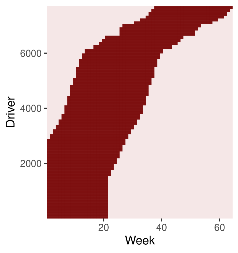
(a) Event Study With Staggered Entry

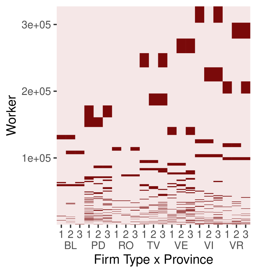
(b) Bipartite Match Outcomes

Figure 1.1: Each of these figures illustrates which outcomes, corresponding to columns, are observed for which units, corresponding to units, in two real-world panel datasets. A given coordinate is colored dark red if the outcome corresponding to the coordinate’s column is observed for the unit corresponding to the coordinate’s row and is colored light red otherwise. Figure 1(a) is generated using data from the longitudinal congestion pricing study studied in Ater . (), while Figure 1(b) is constructed from the VWH Italian matched employer-employee dataset, as detailed in Section 5.1.

Figure 1.1 provides two empirical examples of complex outcome missingness patterns under which the methods developed in this paper can be applied. As an example of an event study setting, Figure 1(a) displays the control potential outcome observation pattern from Ater, Shany, Ross, Turkel  Vasserman (), which evaluates the effect of a government-run usage-based congestion pricing incentive on the driving behavior of several thousand Israeli drivers from January of 2020 through July of 2021. As can be seen in Figure 1(a), drivers were recruited for observation in a staggered fashion over time and received treatment after a non-random 20 weeks of monitoring. As an example of a bipartite matching setting, Figure 1(b) shows which of a subset of Italian workers in the Veneto Worker Histories (VWH) dataset received wages in each of seven provinces and three firm types within each province between 1991 and 2001; see Section 5.1 for details.

In both cases, outcome missingness patterns are credibly determined by unobserved characteristics of units that also affect outcomes. In Figure 1(a)’s setting, it is possible that drivers who would benefit more from the treatment like remote workers joined the study earlier, while in Figure 1(b)’s setting, workers likely live in the regions with job opportunities that would pay them the highest wages. In addition, the TWFE model’s restriction that unit-level heterogeneity does not affect how outcomes differ within units is plausibly unrealistic in both examples. In Figure 1(a)’s setting, drivers in remote-work-compatible occupations plausibly changed their commuting patterns differently in response to COVID-19 lockdowns than drivers whose occupations required continued in-person work. In Figure 1(b)’s setting, if industries are unequally distributed across space, workers whose skills are disproportionately valued by the industries in some region might receive higher wages there than if they lived in a region without those industries. Finally, in both examples, only a small number of outcomes are observed per unit relative to the number of units in each sample.

Our identification strategy for counterfactual outcome means in short panels with missing outcomes is based on a novel type of matrix we call an Aggregated Projection Matrix (APM). Surprisingly, any basis for an APM’s null space serves as a collection of the factor vectors corresponding to all outcomes with respect to the same basis. To construct an APM, we first group units into cohorts that share the same sets of observed outcomes. Next, we use the observations for each cohort to recover the collections of factors corresponding to each cohort’s observed outcomes up to cohort-specific bases using any of the myriad of existing approaches for identifying factors in short panels without missing data, e.g. those discussed in Section 4.3. Finally, we aggregate the projection matrices onto the spans of the matrices whose non-zero rows are the recovered cohort-specific factors in a particular manner into an APM. Having identified the factors corresponding to all outcomes via the APM’s null space, we then leverage an idea proposed in various forms in Imbens . (2021), Brown  Butts (2022), and Agarwal, Shah  Shen (2023) to recover cohort-specific outcome means by learning a linear relationship between the factors corresponding to the observed and missing outcomes in the target cohort.

We prove that our approach identifies the collection of factors corresponding to every outcome so long as a particular graph is connected, where the graph is constructed based on the overlap in observed outcomes between pairs of cohorts. Importantly, our method accommodates more general missingness patterns than other approaches for short panels, and it automatically stitches together different pieces of identifying information each used in isolation by existing methods. It also does not make assumptions on how units select into cohorts based on their low-dimensional unobserved confounders. Moreover, unlike approaches designed for long panels with many observed outcomes per unit, our approach does not require exact recovery of those unobserved confounders, and is thus not vulnerable to the incidental parameter problem (Neyman  Scott, 1948; T. Lancaster, 2000).

We also translate this identification strategy into a plug-in estimator. In particular, we compute an estimated APM using estimates of cohort-specific factors constructed using the data corresponding to each cohort. We then use the rows of the matrix of eigenvectors corresponding to the smallest eigenvalues of the estimated APM as estimates of the factor vectors corresponding to all outcomes. As such, our estimator is quite simple to compute. In an asymptotic regime in which the number of outcomes remains fixed as the cross-sectional dimension of the panel grows, we show that this estimator is consistent and asymptotically normal, and that a weighted bootstrap procedure provides valid asymptotic inference. These results rely on an exact, first-order expansion of the operator mapping a symmetric matrix into the projection matrix onto the space spanned by some subset of its eigenvectors. To our knowledge, this expansion is new.

Finally, we demonstrate the empirical performance of our estimator via a semi-synthetic simulation study based on the VWH dataset of wages earned by workers at different types of firms in the Veneto region of Italy. To define outcomes, we cluster firms within each province into three types by their weekly wage distributions as in Bonhomme . (2019) and define a worker’s outcome corresponding to a given type of firm in a given province as the average weekly wage they would earn were they to work for that type of firm in that province. Importantly, the outcome missingness pattern for this setting, which we illustrate in Figure 1(b), is complex enough to preclude counterfactual outcome mean estimation using existing factor-model-based methods.

To assess the accuracy of our factor-model-based procedure relative to an estimator based on a TWFE model of counterfactual outcome means, we mask an observed outcome for some cohort of units in our data and resample units from these masked data to construct synthetic datasets. We then compute various error metrics of both estimators of the artificially hidden cohort outcome’s mean across resampled synthetic datasets. Across many masked cohort outcomes, our procedure consistently delivers outcome mean estimates with lower bias and root mean squared error than the TWFE-based estimator. In line with Bonhomme . (2019), our simulation results suggest that complementarities between workers and firms do affect wages.

1.1 Related Work

Recently, a variety of methods have been proposed that can be used to estimate and conduct inference on a target cohort outcome mean by aggregating accurate imputations of individual-level factor structure estimates for units in the target cohort constructed using data on units’ observed outcomes, e.g. Gobillon  Magnac (2016); Xu (2017); Athey . (2021); J. Bai  Ng (2021); Arkhangelsky . (2021); Ben-Michael . (2022); Xiong  Pelger (2023); Agarwal, Dahleh . (2023); Chernozhukov . (2023); Farias . (2021); Choi  Yuan (2023); Choi . (2023); Arkhangelsky  Hirshberg (2023); Fernández-Val . (2021). These methods require the number of outcomes and maximum number of observed outcomes per cohort to grow as the number of units grows, since outcome-specific factor vectors can be estimated consistently using variation across many units and unit-specific loading vectors can be estimated consistently using variation across many outcomes. However, under our asymptotic regime of interest in which only a finite number of outcomes are observed per unit, we cannot recover each unit’s loadings without bias that persists as the number of units grows and does not average out to zero across units in the population, precluding averages across imputations. Further, this bias can contaminate the outcome-specific factor estimates themselves even if the cross-sectional panel dimension is large (Neyman  Scott, 1948; T. Lancaster, 2000). On the other hand, when the missingness pattern is complicated, a restriction on the missingness mechanism, such as missing at random, or knowledge of it, such as the probability of jointly observing each pair of outcomes, is often needed even in long panels (Xiong  Pelger, 2023). However, this information is typically unavailable and hard to come by in settings like those illustrated in Figure 1.1.

Instead, we build on an approach suggested in various forms in Imbens . (2021), Brown  Butts (2022), and Agarwal, Shah  Shen (2023): given just factor vectors corresponding to all outcomes, we can construct a linear combination of the target cohort’s observed outcome means that equals the target cohort outcome mean. Imbens . (2021) call any such linear combination a bridge function to highlight the connections they make between this setting and the proximal causal inference literature (Miao ., 2018; Deaner, 2018).

The bridge function-based identification strategy was originally developed in the context of settings with a block missingness pattern, as illustrated in Figure 1(a). In these settings, there exists a “reference” cohort of units for whom all outcomes are observed, so any method for identifying and estimating a factor model without missing data can be applied to the data from the reference cohort to recover the factor vectors for all outcomes with respect to the same basis; we discuss several such methods in Section 4.3.

The bridge function approach can still be applied to identify some cohort outcome means under even more general missingness patterns so long as a reference cohort exists. In event study settings with staggered treatment adoption, so long as there is a “never-treated” group of units for whom all control potential outcomes are observed, these units can be used as a reference cohort, and the approaches developed in Callaway  Karami (2023), Brown  Butts (2022), Brown . (2023), and Callaway  Tsyawo (2023) identify and yield consistent estimates of outcome means when the number of outcomes remains fixed as the cross section’s size grows. Agarwal, Dahleh . (2023) show that the bridge function approach can be applied to identify some cohort outcome means in even more general settings like the one illustrated in Figure 1(b) by finding block missingness patterns embedded within the broader outcome missingness pattern.

However, several important challenges remain in estimating and conducting valid inference on cohort outcome means under factor models that are common in empirical settings such as those illustrated in Figure 1.1. First, many embedded block missingness patterns may exist within a broader missingness pattern to identify some cohort outcome means, and it is unclear how one should combine information gleaned from each of them in a computationally efficient manner to improve estimate precision. Second and more importantly, embedded block missingness patterns cannot always be found to identify all cohort outcome means. Our identification and estimation approach automatically combines information about factor vectors from all cohorts to identify and estimate cohort outcome means without requiring embedded block missingness patterns to exist.

The graph connectivity assumption underlying our identification argument bears resemblance to those made in several papers in the rich literature on fixed-effect-like models of bipartite match outcomes under strict exogeneity, e.g. Abowd . (2002); Jochmans  Weidner (2019); Bonhomme . (2019); Hull (2018); see Bonhomme (2020) for a review. As it happens, we show in Appendix D.2 that, while our connectivity requirement enables identification for general numbers of factors and loadings, in the special case where the factors and loadings are unidimensional, our assumption is essentially equivalent to theirs.

Our consistency and asymptotic linearity results are also related to a large literature applying perturbation-theoretic results to characterize the concentration of eigenspaces of random matrices. To characterize the asymptotic distributions of eigenspaces of estimated matrices as we do in this paper, the concentration guarantees implied by canonical zeroth-order approximation bounds like the Davis–Kahan theorem (see Yu . (2015) for a convenient version) are too coarse. In our paper, we instead characterize the asymptotic distributions of estimated eigenspaces and the estimators on which they depend by deriving a non-asymptotic, first-order eigenspace projection operator expansion based on Kato’s integral (Kato, 1949). Several other papers have also applied Kato’s integral to derive concentration results for eigenspaces of random matrices with (approximately) independent entries, e.g. Oliveira (2010); Mao . (2021); Lei (2020). Relatedly, Simons (2023) applies an asymptotic linearization of the eigenspace operator from Jg. Sun (1991) to derive asymptotically valid hypothesis tests concerning eigenspaces of an estimated, potentially non-symmetric matrix.

2 Setup and Intuition

2.1 Setup

We describe our setting of interest formally as follows. Researchers observe a large, i.i.d. sample of $N$ units, and each unit has $T$ outcomes associated with them, where $Y_{it}^{*}$ denotes unit $i$’s outcome $t$. Importantly, not all outcomes are observed for each unit. To describe which outcomes are observed, we group units into $C$ cohorts, where $C_{i}$ denotes unit $i$’s cohort. For the units in cohort $c$, we only observe the outcomes with indices $t$ in a subset of all outcome indices $\mathcal{T}_{c}\subseteq\{1,\dotsc,T\}$. To distinguish between observed and missing outcomes, we define $Y_{it}=Y_{it}^{*}$ if outcome $t$ is observed for unit $i$ (i.e. if $t\in\mathcal{T}_{C_{i}}$) and $Y_{it}=\emptyset$ otherwise. Given these unbalanced panel data, researchers are often interested in estimating aggregations of cohort-level outcome means:

$$\mu_{ct}\coloneqq\operatorname{\mathbb{E}}[Y_{it}^{*}~{}|~{}C_{i}=c].$$ (2.1)

We refer to $\mu_{ct}$ as a counterfactual outcome mean since outcome $t$ may not be observed for the units in cohort $c$. To model the small number of observed outcomes per unit in our asymptotic theory in Section 4.2, we will focus on the case where the number of outcomes $T$ remains bounded as the sample size $N$ grows.

The setup described above encapsulates several kinds of causal panel data analyses. In event study settings like Figure 1(a)’s, $Y_{it}^{*}$ is unit $i$’s control potential outcome had they not yet been treated by period $t$, units belong to cohort $c$ if they first received treatment at time $c$, and researchers typically estimate aggregations of average treatment effects on the units in each cohort like dynamic effects across post-treatment periods. In bipartite matching settings like Figure 1(b)’s, $Y_{it}^{*}$ is “row-type” unit $i$’s outcome if matched with “column-type” unit $t$, row-type units belong to the same cohort if they were matched with the same set of column-type units, and researchers typically estimate aggregations of $\mu_{ct}$s that characterize the degree to which row-type and column-type unit heterogeneity affect differences in average observed outcomes across column-type units.

We assume outcomes $Y_{it}^{*}$ are generated according to a rank-$r$ factor model, i.e. that outcomes are determined by the inner product of a fixed vector of outcome-specific factors $\gamma_{t}\in\operatorname{\mathbb{R}}^{r}$ and a vector of unit-specific loadings $\lambda_{i}\in\operatorname{\mathbb{R}}^{r}$ plus an error term $\operatorname{\varepsilon}_{it}$ that has zero mean given unit $i$’s loadings and cohort membership $C_{i}$:

$$Y_{it}^{*}=\gamma_{t}^{\prime}\lambda_{i}+\operatorname{\varepsilon}_{it},\quad\operatorname{\mathbb{E}}[\operatorname{\varepsilon}_{it}~{}|~{}\lambda_{i},C_{i}]=0.$$ (2.2)

As in other fixed-effect-like models like the TWFE model or the static model studied in Bonhomme . (2019), the assumption that $\operatorname{\varepsilon}_{it}$ is mean-independent of cohort membership $C_{i}$ conditional on loadings $\lambda_{i}$ implies that only the coordinates of $\lambda_{i}$ can serve as confounders that affect both units’ cohort memberships and their outcomes. By considering the factor vectors $\gamma_{t}$ to be fixed, we essentially condition our inference on the factors $\{\gamma_{t}:t=1,\dotsc,T\}$. If we consider the factors $\gamma_{t}$ to be random, the residual mean condition in (2.2) can be read as $\operatorname{\mathbb{E}}[\operatorname{\varepsilon}_{it}~{}|~{}\lambda_{i},C_{i},\gamma_{1},\dotsc,\gamma_{T}]=0$.

Throughout this paper, we assume the rank of the factor model $r<T$ is known. In keeping with other methods based on fixed-effect-like models of short panels with unobserved heterogeneity (e.g. Bonhomme . (2019)), we suggest that researchers using our method assess the robustness of their results to different values of $r$, insofar as the cohort outcome means they would like to estimate are identified given that choice of $r$, as discussed in Section 4.1. The simulation study in Section 5.2 that assesses the performance of our estimation procedure on held-out cohort outcomes also provides a blueprint for assessing the relative performance of our estimator given different choices of $r$.

2.2 Intuition

Broadly, our approach for identifying and estimating a target cohort outcome mean $\mu_{c^{*}t^{*}}$ proceeds in two stages. First, we recover all of the factor vectors across outcomes with respect to a common basis. Then, we use the factor vectors corresponding to the target cohort’s observed outcomes and the target outcome to extrapolate from the target cohort’s observed outcome means to the target outcome mean. To highlight the additional challenge posed by the first stage, we proceed by first providing intuition for the second stage in a setting where the first stage happens to be straightforward.

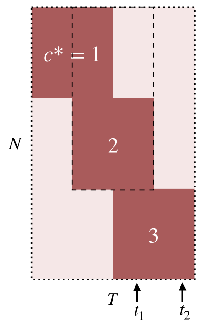
(a) Block Missingness Pattern

(b) Three-Cohort Staircase Pattern

Figure 2.1: This figure illustrates two stylized outcome missingness patterns, where, similarly to Figure 1.1, a coordinate is colored dark red if the outcome corresponding to the coordinate’s column is observed for the unit corresponding to the coordinate’s and is colored light red otherwise. We use numbers to indicate the cohorts of units for whom different blocks of outcomes are observed.

In particular, we focus on a simple, three-cohort outcome missingness pattern illustrated in Figure 1(b) and consider estimating a target cohort outcome mean $\mu_{c^{*}t^{*}}$, where $c^{*}=1$ is the target cohort and $t^{*}=t_{1}$ is the target outcome. Suppose also that we have access to the factors $\gamma_{t}$ for all outcomes. Then, under regularity conditions, there exist many vectors of coefficients $\beta$ we can construct such that a linear combination of the factor vectors for the target cohort $c^{*}$’s observed outcomes with those coefficients equals the factor vector $\gamma_{t^{*}}$ corresponding to the target outcome $t^{*}$:

$$\sum_{t\in\mathcal{T}_{c^{*}}}\beta_{t}\gamma_{t}=\gamma_{t^{*}}.$$ (2.3)

As it happens, the same linear combination of the target cohort’s observed outcome means $\operatorname{\mathbb{E}}[Y_{it}~{}|~{}C_{i}=c^{*}]$ for $t\in\mathcal{T}_{c^{*}}$ will equal the target cohort’s target outcome mean (Agarwal, Shah  Shen, 2023; Imbens ., 2021; Brown  Butts, 2022):

$$\sum_{t\in\mathcal{T}_{c^{*}}}\beta_{t}\underbrace{\operatorname{\mathbb{E}}[Y_{it}~{}|~{}C_{i}=c^{*}]}_{=\operatorname{\mathbb{E}}[Y_{it}^{*}~{}|~{}C_{i}=c^{*}]}\overbrace{=}^{\text{by \eqref{eq:factor_model}}}\sum_{t\in\mathcal{T}_{c^{*}}}\beta_{t}\gamma_{t}^{\prime}\operatorname{\mathbb{E}}[\lambda_{i}~{}|~{}C_{i}=c^{*}]\overbrace{=}^{\text{by \eqref{eq:bridge_function_extrapolation}}}\gamma_{t^{*}}^{\prime}\operatorname{\mathbb{E}}[\lambda_{i}~{}|~{}C_{i}=c^{*}]\overbrace{=}^{\text{by \eqref{eq:factor_model}}}\mu_{c^{*}t^{*}}.$$ (2.4)

In keeping with Imbens . (2021), we refer to any linear transformation $\beta^{\prime}$ where $\beta$ satisfies (2.3) as a bridge function.

Turning to the first stage of our approach, we now discuss how to recover the factors $\gamma_{t}$ used to construct bridge functions $\beta^{\prime}$ via solutions to (2.3). A well known fact in the rich literature on factor models is that, even in settings where all outcomes are observed, only a common linear transformation $Q\gamma_{t}$ of each factor vector $\gamma_{t}$ can be identified, where $Q$ is an unknown, $r\times r$ invertible matrix we refer to as a basis.

Luckily, the bridge function approach renders this basis indeterminacy immaterial when our target cohort is $c^{*}=1$ and our target outcome is $t^{*}=t_{1}$. To see why, note that in this case, there exists a “reference” cohort $2$ of units for whom we observe both the target outcome $t_{1}$ and some of the outcomes also observed for the units in the target cohort (Agarwal, Dahleh ., 2023; Brown  Butts, 2022). In other words, the set of units and outcomes inside the black dashed rectangle in Figure 1(b) constitutes a block missingness pattern like the one shown in Figure 1(a) embedded within the broader outcome missingness pattern in Figure 1(b). Then, under a variety of additional assumptions discussed in Section 4.3, a myriad of methods can still be applied using just the data from cohort $2$ to recover transformed factor vectors $Q\gamma_{t_{1}}$ corresponding to the target outcome and $Q\gamma_{t}$ for $t\in\mathcal{T}_{1}\cap\mathcal{T}_{2}$ corresponding to the overlapping observed outcomes between cohorts $1$ and $2$, where $Q$ is a common basis. Since the set of valid bridge functions $\beta^{\prime}$ satisfying (2.3) is invariant to multiplying all of the factor vectors $\gamma_{t}$ by the same basis matrix $Q$, the second stage of our identification approach remains unaffected.

Unfortunately, when our target outcome is instead $t^{*}=t_{2}$, no reference cohort exists for whom we observe both the target outcome $t_{2}$ and any observed outcomes for our target cohort $c^{*}=1$. As such, there is no subset of the data we can directly use to recover the factors corresponding to the target outcome and the target cohort’s observed outcomes with respect to the same basis. Instead, again under different sets of additional assumptions (see Section 4.3), we can only use the observed outcomes of units in each cohort $c$ to recover transformed factor vectors $\tilde{\gamma}_{ct}\coloneqq Q_{c}\gamma_{t}$ corresponding to cohort $c$’s observed outcomes $t\in\mathcal{T}_{c}$ with respect to a cohort-specific basis $Q_{c}$. In other words, at best, we can recover cohort-specific factor vectors that are “misaligned.” To be able to find bridge functions that satisfy (2.3), we need to construct an aligned set of factor vectors expressed with respect to a common basis that correspond to both the target outcome $t_{2}$ and the target cohort’s observed outcomes $t\in\mathcal{T}_{1}$.

To describe our solution to this factor vector misalignment problem, we define some additional notation. First, stack the factor vectors $\gamma_{t}$ row-wise into a $T\times r$ matrix $\Gamma$, and stack the cohort-specific transformed factor vectors $\tilde{\gamma}_{ct}$ recovered from the data for cohort $c$ into the $T\times r$ matrix $\tilde{\Gamma}_{c}$, where the $t$-th row of $\tilde{\Gamma}_{c}$ equals $\tilde{\gamma}_{ct}=Q_{c}\gamma_{t}$ if outcome $t$ is observed for the units in cohort $c$ and a vector of zeros otherwise. In addition, let $E_{c}$ be the $T\times T$ diagonal matrix whose $t$-th diagonal entry is one if outcome $t$ is observed for cohort $c$, i.e. $t\in\mathcal{T}_{c}$, and zero otherwise. Finally, for any matrix $M$, we denote the projection matrix onto $M$’s column space by $\Pi(M)\coloneqq M(M^{\prime}M)^{+}M^{\prime}$, where $(M^{\prime}M)^{+}$ is the Moore-Penrose pseudo-inverse of $M^{\prime}M$.

Armed with this notation, we can now describe the two insights that underpin our solution to the factor vector alignment problem introduced above. First, since the column space of $\tilde{\Gamma}_{c}=E_{c}\Gamma Q_{c}^{\prime}$ does not depend on $Q_{c}$, the projection matrix $\Pi(\tilde{\Gamma}_{c})$ is the same as the projection matrix $\Pi(E_{c}\Gamma)$ onto the column space of the matrix $E_{c}\Gamma$ whose non-zero rows are exactly the true factor vectors corresponding to cohort $c$’s observed outcomes. Thus, the projection matrix $\Pi(\tilde{\Gamma}_{c})$ derived from cohort $c$’s data provides a unique representation of the available information about the factor vectors corresponding to cohort $c$’s observed outcomes free from contamination by the cohort-specific $Q_{c}$.

Given the cohort-specific projection matrices $\Pi(\tilde{\Gamma}_{c})$, we then must aggregate them in such a way so as to recover the factor vectors $\gamma_{t}$ defined with respect to some common basis. Along these lines, our second key observation is that the column space of $\Gamma$ is a subset of the null space of the matrix $E_{c}-\Pi(\tilde{\Gamma}_{c})=E_{c}-\Pi(E_{c}\Gamma)$ for each cohort $c$. To leverage this insight, we define we define the Aggregated Projection Matrix (APM) operator as follows for any $C$ matrices $\Gamma_{1},\dotsc,\Gamma_{C}\in\operatorname{\mathbb{R}}^{T\times r}$:

$$A(\Gamma_{1},\dotsc,\Gamma_{C})\coloneqq\sum_{c=1}^{C}\left(E_{c}-\Pi(\Gamma_{c})\right).$$ (2.5)

Despite its name, $A(\Gamma_{1},\dotsc,\Gamma_{C})$ is not itself a projection matrix in general. However, since $A(\tilde{\Gamma}_{1},\dotsc,\tilde{\Gamma}_{c})$ is by definition the sum of the matrices $E_{c}-\Pi(\tilde{\Gamma}_{c})$ across cohorts $c$, the column space of $\Gamma$ must lie in the null space of $A(\tilde{\Gamma}_{1},\dotsc,\tilde{\Gamma}_{c})$ as well. In Section 4.1, we show that, perhaps surprisingly, so long as there is sufficient overlap between the observed outcomes across pairs of cohorts, the null space of $A(\tilde{\Gamma}_{1},\dotsc,\tilde{\Gamma}_{c})$ is in fact exactly the column space of $\Gamma$. Thus, the rows of any basis matrix for the null space of $A$ can serve as valid factor vectors when applying the bridge function identification strategy.

3 Estimation and Inference Procedure

Having provided intuition for the conceptual underpinnings of our approach, we now introduce our general estimation and inference procedure, which has four high-level steps. First, we consider the data corresponding to units in each cohort separately and use them to estimate the factors corresponding to the observed outcomes for each cohort. Second, we aggregate these cohort-specific factor estimates into a particular matrix whose eigendecomposition yields valid estimates of the factors corresponding to all outcomes. Third, given those factor estimates, for each cohort, we construct the minimum norm bridge function that consistently extrapolates from that cohort’s observed outcome means to all target outcome means. Finally, we conduct valid inference on cohort outcome means by taking advantage of the asymptotic normality of our estimator.

We now describe our procedure in more detail, beginning with step two outlined above. We assume for now that for each cohort $c$, we have access to estimates $\hat{\gamma}_{ct}$ of the factor vectors corresponding to each outcome $t\in\mathcal{T}_{c}$ observed for cohort $c$. In Section 4.3, we discuss a variety of methods that exist for constructing valid cohort-specific factor vector estimates under different sets of additional assumptions beyond the factor model (2.2). Importantly, most estimators cohort-specific factor vectors $\tilde{\gamma}_{ct}$ require minimal computational overhead for small $T$, and they can be computed in parallel across cohorts using subsets of the data associated with each cohort. We then stack these cohort-specific estimates into the $T\times r$ matrix $\hat{\Gamma}_{c}$ whose $t$-th row is $\hat{\gamma}_{ct}$ if $t\in\mathcal{T}_{c}$, i.e. if outcome $t$ is observed for the units in cohort $c$ and a vector of zeros otherwise.

Given cohort-specific estimated factor matrices $\hat{\Gamma}_{1},\dotsc,\hat{\Gamma}_{C}$, the second step of our procedure consists of constructing the estimated APM $\hat{A}\coloneqq A(\hat{\Gamma}_{1},\dotsc,\hat{\Gamma}_{C})$ and computing its eigendecomposition. Because $T$ is typically small in settings in which we envision our method will be applied, this step can be done extremely quickly using the myriad of optimized eigendecomposition routines available in most programming languages. Let $\hat{\Gamma}$ be the $T\times r$ matrix whose columns are eigenvectors corresponding to the $r$ smallest eigenvalues of $\hat{A}$; as we show in Section 4.2, row $t$ of $\hat{\Gamma}$ is a consistent estimate of the factor vector $\gamma_{t}$ with respect to a particular error metric.

Describing the third step of our procedure requires several more definitions. Collect unit $i$’s observed outcomes into the vector $Y_{i}\coloneqq(Y_{i1},\dotsc,Y_{iT})^{\prime}$, and note that although $Y_{i}$ has undefined entries corresponding to unobserved outcomes, all entries of the vector $E_{C_{i}}Y_{i}$ are well-defined since the entries corresponding to the unobserved outcomes are zero. We also let $N_{c}\coloneqq\sum_{i=1}^{N}\mathbbm{1}\{C_{i}=c\}$ denote the number of units in cohort $c$. We can then define our estimator of the vector $\mu_{c^{*}}\in\operatorname{\mathbb{R}}^{T}$ whose $t$-th entry is the target cohort $c^{*}$’s mean value of outcome $t$, $\mu_{c^{*}t}$:

$$\hat{\mu}_{c^{*}}\coloneqq\hat{\Gamma}\left(E_{c^{*}}\hat{\Gamma}\right)^{+}\cdot\frac{1}{N_{c^{*}}}\sum_{i=1}^{N}\mathbbm{1}\{C_{i}=c^{*}\}E_{C_{i}}Y_{i}.$$ (3.1)

Given that $\hat{\mu}_{c^{*}}$ is simply a vector of least-norm solutions to underdetermined linear equations, it can also be computed efficiently in most programming languages.

Often, researchers are actually interested in estimating a known, vector-valued function $\theta\coloneqq h(\mu,\eta)$ of cohort outcome means $\mu\coloneqq(\mu_{1}^{\prime},\dotsc,\mu_{C}^{\prime})^{\prime}$, along with a vector of nuisance parameters $\eta$ that are estimable from the data. For example, in event study settings, it is common to report average effects of a treatment across different numbers of time periods relative to units’ treatment times. As introduced in Callaway  Sant’Anna (2021) and L. Sun  Abraham (2021) and reviewed in Example D.1 of Appendix D.1, we can express these estimands as weighted averages of the differences between each cohort’s average control potential outcome means $\mu_{c}$ and their observed, treated potential outcome means (part of $\eta$), where the weights are determined by the relative sizes of each cohort (also part of $\eta$).

In the context of bipartite match data on patients’ health outcome when living in different geographic areas, Finkelstein . (2016) suggest an approach to attributing shares of the differences in average health outcomes across regions to people and places that can be expressed in the form $h(\mu,\eta)$, albeit based on a TWFE model of match outcomes. In Example D.2 of Appendix D.1, we discuss nonparametric analogs of their estimands of the form $h(\mu,\eta)$ that do not depend on a particular model of outcomes, but that can be estimated under the factor model (2.2) using our procedure.

Given $\theta$’s relevance in applied contexts, as an extension of the third step of our procedure, we compute a plug-in estimate $\hat{\theta}\coloneqq h(\hat{\mu},\hat{\eta})$ of $\theta$, where the vector $\hat{\mu}\coloneqq(\hat{\mu}_{1}^{\prime},\dotsc,\hat{\mu}_{C}^{\prime})^{\prime}$ collects the cohort outcome mean vector estimates $\hat{\mu}_{c}$ defined in (3.1) across cohorts, and $\hat{\eta}$ is an estimate of the nuisance parameter vector $\eta$. For convenience, we summarize the three steps of our estimation procedure in Algorithm 1.

Data: $\{(C_{i},Y_{i})\}_{i=1}^{N}$

1 for $c\in\{1,\dotsc,C\}$ do

       Compute cohort-specific factor estimates $\hat{\gamma}_{ct}$ for $t\in\mathcal{T}_{c}$ (see Section 4.3)

       Construct a $T\times r$ matrix $\hat{\Gamma}_{c}$ with row $t$ equalling $\hat{\gamma}_{ct}$ if $t\in\mathcal{T}_{c}$, and $\operatorname{\mathbf{0}}_{r}$ otherwise

      

end for

2Construct estimated APM $\hat{A}=P(\hat{\Gamma}_{1},\dotsc,\hat{\Gamma}_{C})$ as in (2.5)

3 Compute $T\times r$ matrix $\hat{\Gamma}$ of eigenvectors corresponding to $\hat{A}$’s $r$ smallest eigenvalues

4 for $c\in\{1,\dotsc,C\}$ do

       Compute outcome mean estimate vector $\hat{\mu}_{c}$ for cohort $c$ as in (3.1)

      

end for

5Compute estimate $\hat{\eta}$ of nuisance parameters $\eta$ necessary for estimating $\theta$

6 Compute plug-in target parameter estimate $\hat{\theta}=h(\hat{\mu},\hat{\eta})$, where $\hat{\mu}=(\hat{\mu}_{1}^{\prime},\dotsc,\hat{\mu}_{C}^{\prime})^{\prime}$

Algorithm 1 Estimation

For the fourth and final step of our procedure, we construct simultaneous $1-\alpha$ confidence intervals for the $p$ coordinates of $\theta$. For simplicity and numerical stability, we construct these intervals via a Bayesian bootstrap (Rubin, 1981). To describe how we construct these intervals, we introduce more notation. Given a vector of $N$ non-negative weights $W\coloneqq(W_{1},\dotsc,W_{N})^{\prime}$ that sum to one, we will assume that both our cohort-specific factor matrix estimators $\hat{\Gamma}_{ct}$ and our nuisance parameter estimator $\hat{\eta}$ can be adapted to accommodate non-uniform sampling weights $W$, which we denote $\hat{\Gamma}_{c}(W)$ and $\hat{\eta}(W)$, respectively; see Section 4.3 for details on weighted versions of $\hat{\Gamma}_{c}$. We also let $\hat{A}(W)\coloneqq A(\hat{\Gamma}_{1}(W),\dotsc,\hat{\Gamma}_{C}(W))$ denote the APM constructed from the weighted, estimated cohort-specific factor matrices $\hat{\Gamma}_{1}(W),\dotsc,\hat{\Gamma}_{C}(W)$, we let $\hat{\Gamma}(W)$ denote the equivalent of $\hat{\Gamma}$ constructed from the weighted estimated APM $\hat{A}(W)$, and we let $\hat{\mu}_{c}(W)$ denote the weighted equivalent of $\hat{\mu}_{c}$ defined as follows:

$$\hat{\mu}_{c}(W)\coloneqq\hat{\Gamma}(W)\left(E_{c}\hat{\Gamma}(W)\right)^{+}\sum_{i=1}^{N}\frac{W_{i}\mathbbm{1}\{C_{i}=c\}}{\sum_{j=1}^{N}W_{j}\mathbbm{1}\{C_{j}=c\}}E_{C_{i}}Y_{i}.$$ (3.2)

A weighted version of our plug-in estimator of $\hat{\theta}$ is $\hat{\theta}(W)\coloneqq h(\hat{\mu}(W),\hat{\eta}(W))$, where $\hat{\mu}(W)$ is the weighted analog of $\hat{\mu}$. Before continuing, we note that under uniform weights $W_{1}=\dotsc=W_{N}=\frac{1}{N}$, all of the quantities defined previously in this paragraph equal their unweighted counterparts defined above.

Data: $\{(C_{i},Y_{i})\}_{i=1}^{N}$, number of bootstrap samples $M$.

1 for $m\in\{1,\dotsc,M\}$ do

       Sample $\xi_{m1},\dotsc,x_{mN}\operatorname{\stackrel{{\scriptstyle i.i.d.}}{{\sim}}}\mathrm{Exp}(1)$

       Construct weight vector $W_{m}\coloneqq(W_{m1},\dotsc,W_{mN})^{\prime}$ with $W_{mi}\coloneqq\xi_{mi}/\sum_{j=1}^{N}\xi_{mj}$

       for $c\in\{1,\dotsc,C\}$ do

             Compute weighted cohort outcome mean estimate vector $\hat{\mu}_{c}(W_{m})$ as in (3.2) (using Algorithm 1 with weighted analogs)

            

       end for

      Compute weighted nuisance parameter estimates $\hat{\eta}(W_{m})$

       Compute weighted target parameter estimate $\hat{\theta}^{*}_{m}=h(\hat{\mu}(W_{m}),\hat{\eta}(W_{m}))$

      

end for

2for $j\in\{1,\dotsc,p\}$ do

       Compute estimate $\hat{\sigma}_{j}$ of $\hat{\theta}$’s standard error, e.g. as in (3.3)

      

end for

3Compute estimated critical value $\hat{q}_{1-\alpha}$ as in (3.4)

4 Compute simultaneous $1-\alpha$ confidence intervals $\hat{\mathcal{C}}_{j}$ as in (3.5)

Algorithm 2 Weighted Bootstrap Inference

Given this notation, our inference procedure proceeds as follows. First, for each iteration $m$ of a large number $M$ of repetitions, we take $N$ i.i.d. draws $\xi_{m1},\dotsc,\xi_{mN}$ from the $\mathrm{Exponential}(1)$ distribution, construct a vector $W_{m}\coloneqq(W_{m1},\dotsc,W_{mN})^{\prime}$ of $N$ normalized weights $W_{mi}\coloneqq\xi_{mi}/\sum_{j=1}^{N}\xi_{mj}$, and compute a weighted target parameter estimate $\hat{\theta}^{*}_{m}\coloneqq\hat{\theta}(W_{m})$. Next, for each coordinate $j\in\{1,\dotsc,p\}$ of $\theta$, we compute an estimate $\hat{\sigma}_{j}$ of the standard error of $\hat{\theta}_{j}$, e.g.

$$\hat{\sigma}_{j}\coloneqq\frac{q_{0.75}(\hat{\theta}^{*}_{1j},\dotsc,\hat{\theta}^{*}_{Mj})-q_{0.25}(\hat{\theta}^{*}_{1j},\dotsc,\hat{\theta}^{*}_{Mj})}{q_{0.75}(Z)-q_{0.25}(Z)},$$ (3.3)

where we let $q_{\zeta}(x_{1},\dotsc,x_{M})$ denote the $\zeta$th quantile across scalars $x_{1},\dotsc,x_{M}$, and we let $q_{\zeta}(Z)$ denote the $\zeta$th quantile of the standard Gaussian distribution. Finally, we let $\hat{q}_{1-\alpha}$ denote the following estimated critical value:

$$\hat{q}_{1-\alpha}\coloneqq q_{1-\alpha}(z^{*}_{1},\dotsc,z^{*}_{M}),\quad z^{*}_{m}\coloneqq\max_{j\in\{1,\dotsc,p\}}\left\lvert\hat{\theta}^{*}_{mj}\big{/}\hat{\sigma}_{j}\right\rvert,$$ (3.4)

and we define our simultaneous $1-\alpha$ confidence intervals $\hat{\mathcal{C}}_{j}$ for $\theta_{j}$ across $j=1,\dotsc,p$ as follows:

$$\hat{\mathcal{C}}_{j}\coloneqq\left[\hat{\theta}_{j}-\hat{q}_{1-\alpha}\hat{\sigma}_{j},\hat{\theta}_{j}+\hat{q}_{1-\alpha}\hat{\sigma}_{j}\right].$$ (3.5)

For convenience, we summarize the steps of our inference procedure in Algorithm 2.

4 Theoretical Properties

4.1 Identification Given Cohort-Specific Factors

To highlight the contributions of this paper, we assume for now that we have identified the column spaces of the cohort-specific factor matrices $E_{c}\Gamma$:

Assumption 4.1.

The projection matrices $\Pi(E_{c}\Gamma)$ are identified for all cohorts $c=1,\dotsc,C$.

In Section 4.3, we will discuss several sets of additional assumptions standard in the rich literature on factor models under which Assumption 4.1 holds.

To characterize which outcomes our approach can and cannot identify given identified cohort specific factor projection matrices $\Pi(E_{c}\Gamma)$, we define an object we call the Observed Outcome Overlap Graph $\mathcal{G}_{r}$. The graph $\mathcal{G}_{r}$ consists of $C$ vertices, one corresponding to each cohort, and an edge between two distinct cohorts $c_{1}$ and $c_{2}$ if the space spanned by the factor vectors corresponding to the two cohorts’ overlapping observed outcomes $\mathcal{T}_{c_{1}}\cap\mathcal{T}_{c_{2}}$ has at least $r$ dimensions, or formally, if

$$\mathrm{rank}\left(E_{c_{1}}E_{c_{2}}\Gamma\right)=r.$$ (4.1)

While (4.1) is a requirement on the unobserved factor matrix $\Gamma$, we note that a necessary condition that only depends on the known sets of observed outcomes $\mathcal{T}_{c}$ across cohorts is that cohorts $c_{1}$ and $c_{2}$ have at least $r$ overlapping observed outcomes: $\lvert\mathcal{T}_{c_{1}}\cap\mathcal{T}_{c_{2}}\rvert\geq r$. As we show in Appendix D.2, this condition is also sufficient when $r=1$. In Figure E.1, we illustrate $\mathcal{G}_{1}$ for the two empirical examples introduced in Section 1.

Our key requirement to identify all of the outcome means for a given cohort can be stated succinctly in terms of the connectedness of $\mathcal{G}_{r}$:

Assumption 4.2.

The observed outcome overlap graph $\mathcal{G}_{r}$ is connected.

Before continuing, three remarks concerning Assumption 4.2 are in order. First, Assumption 4.2 implies that every cohort must have at least $r$ observed outcomes, and that every factor must affect at least one outcome in every cohort (a proof is provided in Appendix A.1):

Lemma 4.1.

Under Assumption 4.2, $\mathrm{rank}(E_{c}\Gamma)=r$ for all cohorts $c=1,\dotsc,C$.

A consequence of Lemma 4.1 is that our identification, estimation, and inference results hold for the subset of units for whom at least $r$ outcomes are observed, i.e. conditional on $\lvert\mathcal{T}_{C_{i}}\rvert\geq r$.

Second, if $\mathcal{G}_{r}$ is not connected, our identification, estimation, and inference results apply instead to the subset of cohorts belonging to the connected component of $\mathcal{G}_{r}$ that contains the target cohort $c^{*}$ and the subset of outcomes observed for at least one of those cohorts. Third, we show in Appendix D.2 that when $r=1$, Assumption 4.2 is equivalent to typical connectedness assumptions made in the literature on fixed-effect-type models of bipartite network data under strict exogeneity (see Abowd . (2002); Jochmans  Weidner (2019); Bonhomme . (2019); Hull (2018) for examples, and Bonhomme (2020) for a review).

Given identification of the cohort-specific factor projection matrices $\Pi(E_{c}\Gamma)$, we denote the population APM by substituting the population cohort-specific factor matrices $E_{c}\Gamma$ into the APM definition (2.5) as follows:

$$A\coloneqq A(E_{1}\Gamma,\dotsc,E_{c}\Gamma).$$ (4.2)

We are now equipped to state our main identification result:

Theorem 4.2.

Suppose Assumptions 4.1 and 4.2 hold; then the column space of $\Gamma$ is identified by the null space of the APM $A$.

The containment of the column space of $\Gamma$ in the null space of the APM $A$ can be shown succinctly even without Assumption 4.2 (see Footnote 15). However, the containment of the null space of the APM $A$ in the column space of $\Gamma$ under Assumption 4.2 requires a more involved argument, which we provide in Appendix A.2.

Given identification of the column space of the factor matrix $\Gamma$, we can then identify the target cohort’s outcome means via the bridge function approach articulated in Section 3:

Corollary 4.3.

Suppose Assumptions 4.1 and 4.2 hold, and let $\tilde{\Gamma}$ be any basis for the null space of the APM $A$. Then the vector $\mu_{c^{*}}$ of outcome means for cohort $c^{*}$ is identified as follows:

$$\mu_{c^{*}}=\tilde{\Gamma}\left(E_{c^{*}}\tilde{\Gamma}\right)^{+}\operatorname{\mathbb{E}}[E_{c^{*}}Y_{i}~{}|~{}C_{i}=c^{*}].$$ (4.3)

We provide a proof of Corollary 4.3 in Appendix A.3.

Before continuing, we note that, because we impose the factor model functional form (2.2), our identification argument for $\mu_{c}$ does not rely on any support assumptions about the cohort-specific loading distributions $\lambda_{i}~{}|~{}C_{i}=c$, unlike some other approaches to estimating counterfactual outcome means in the presence of unobserved heterogeneity. For example, in the context of event study settings, methods in the Synthetic Control family like Abadie . (2010) and Arkhangelsky . (2021) typically require the average target cohort’s loadings to lie in the convex hull of the loadings of the units in the donor pool. In the context of bipartite match outcomes, Bonhomme . (2019) require every latent type of row-type unit to be matched with every latent type of column-type unit. In Section 4.3, none of the additional sets of assumptions we discuss require overlapping support in the cohort-specific loading distributions for Assumption 4.1 to hold either. As such, our approach is robust to large discrepancies in the unobserved confounding variables across cohorts, so long as the low-rank factor model (2.2) is correctly specified.

4.2 Asymptotic Linearity of $\hat{\mu}_{c}$ Given Cohort-Specific Factors

Having shown how to identify the column space of $\Gamma$ and, by extension, $\mu_{c}$, we now turn to showing that the plug-in estimator described in Section 3 yields asymptotically linear estimates of these parameters. First, we introduce some convenient notation. Let $\mathrm{vec}(M)$ denote the vectorization of the matrix $M$, i.e. the vector containing the columns of the matrix $M$ stacked in order, and let $\hat{\operatorname{\mathbb{E}}}_{N}$ denote the expectation operator with respect to the empirical measure $\hat{P}_{N}$ with sample size $N$.

To highlight the contributions of this paper, as in Section 4.1, we will assume in this section that we are equipped with asymptotically linear estimators $\Pi(\hat{\Gamma})$ of the column spaces of $E_{c}\Gamma$, represented uniquely by $\Pi(E_{c}\Gamma)$:

Assumption 4.3.

For each cohort $c=1,\dotsc,C$, there exists a function $\phi_{c}$ of $C_{i}$ and $Y_{i}$ such that the vectorization of the estimated cohort-specific factor projection matrix $\Pi(\hat{\Gamma}_{c})$ satisfies the following asymptotic expansion as $N\rightarrow\infty$:

$$\sqrt{N}\mathrm{vec}\left(\Pi(\hat{\Gamma}_{c})-\Pi(E_{c}\Gamma)\right)=\sqrt{N}\hat{\operatorname{\mathbb{E}}}_{N}[\phi_{c}(C_{i},Y_{i})]+o_{p}\left(1\right),$$ (4.4)

$\operatorname{\mathbb{E}}[\phi_{c}(C_{i},Y_{i})]=\operatorname{\mathbf{0}}_{T}$, and $\operatorname{\mathbb{E}}\left[\left\lVert\phi_{c}(C_{i},Y_{i})\right\rVert_{2}^{2}\right]<\infty$.

In Section 4.3, we will discuss several sets of additional assumptions standard in the rich literature on factor models under which estimators satisfying Assumption 4.3 exist.

Before continuing, we note that, at first glance, Assumption 4.3 might appear to be chosen simply to imply asymptotic linearity of the empirical APM $\hat{A}$ without much effort, since the population APM $A$ and its plug-in counterpart $\hat{A}$ can be directly expressed as sums of $\Pi(E_{c}\Gamma)$ and $\Pi(\hat{\Gamma}_{c})$ across $c$, respectively. While Assumption 4.3 is certainly convenient for this reason, perhaps more importantly, it is also a weaker requirement on the cohort-specific factor matrix estimators $\hat{\Gamma}_{c}$ than assuming the kind of asymptotic linearity guarantees typically shown under stronger assumptions in the literature on factor estimation, as discussed in more detail in Section 4.3 and Appendix D.3.

Next, we can show that the plug-in estimator $\hat{\Gamma}$ of $\Gamma$ is asymptotically linear in the following sense, where $\otimes$ denotes the Kronecker product:

Theorem 4.4.

Suppose that Assumptions 4.1, 4.2, and 4.3 hold. Then as $N\rightarrow\infty$,

$$\sqrt{N}\mathrm{vec}\left(\Pi(\hat{\Gamma})-\Pi(\Gamma)\right) =\sqrt{N}\hat{\operatorname{\mathbb{E}}}_{N}\left[H\sum_{c=1}^{C}\phi_{c}(C_{i},Y_{i})\right]+o_{p}\left(1\right)$$ (4.5)

where $H$ is the following $T^{2}\times T^{2}$ matrix:

$$H\coloneqq A^{+}\otimes\Pi(\Gamma)+\Pi(\Gamma)\otimes A^{+},$$ (4.6)

$\operatorname{\mathbb{E}}[H\sum_{c=1}^{C}\phi_{c}(C_{i},Y_{i})]=\operatorname{\mathbf{0}}_{T^{2}}$, and $\operatorname{\mathbb{E}}[\lVert H\sum_{c=1}^{C}\phi_{c}(C_{i},Y_{i})\rVert_{2}^{2}]<\infty$.

We provide a proof of Theorem 4.4 in Appendix A.4. Our proof relies on an exact, first-order expansion of the operator mapping a symmetric matrix into the projection matrix onto the space spanned by some subset of its eigenvectors derived using Kato’s integral (Kato, 1949). Since the projection matrix onto the space spanned by a matrix’s columns is a unique representation of that matrix’s column space, this expansion allows us to directly bound the error incurred by $\Pi(\hat{\Gamma})$ as an estimator of the column space of $\Gamma$ under minimal assumptions on the eigenvalues of $A$. Because it is exact, our expansion appears to be new as far as we are aware. Since this expansion may be of independent interest, we provide a self-contained description and proof in Appendix B.

Having shown that our plug-in estimator of the column space of $\Gamma$ is asymptotically linear, we now turn to showing that $\hat{\mu}_{c}$ is therefore also an asymptotically linear estimator of $\mu_{c}$. To do so, we require the following additional regularity conditions on cohort sizes and outcome moments, where $Y_{i}^{*}\coloneqq(Y_{i1}^{*},\dotsc,Y_{iT}^{*})^{\prime}$ denotes the vector that collects unit $i$’s outcomes:

Assumption 4.4.

For all cohorts $c=1,\dotsc,C$, $\operatorname{\mathbb{P}}(C_{i}=c)>0$ and $\operatorname{\mathbb{E}}\left[\lVert Y_{i}^{*}\rVert_{2}^{2}~{}\middle|~{}C_{i}=c\right]<\infty$.

As it happens, we can express $(E_{c}\Gamma)^{+}$ as a known function of $E_{c}$ and $\Pi(\Gamma)$, which enables us to derive a first-order asymptotic expansion of our plug-in estimator $\hat{\mu}_{c}$ with respect to $\Pi(\hat{\Gamma})$. This result implies $\hat{\mu}_{c}$ has exactly our desired properties:

Theorem 4.5.

Suppose that Assumptions 4.1, 4.2, 4.3, and 4.4 hold. Then as $N\rightarrow\infty$,

$$\sqrt{N}(\hat{\mu}_{c^{*}}-\mu_{c^{*}}) =\sqrt{N}\hat{\operatorname{\mathbb{E}}}_{N}\left[\psi_{c^{*}}(C_{i},Y_{i})\right]+o_{p}\left(1\right),$$ (4.7)

$$\psi_{c^{*}}(C_{i},Y_{i}) \coloneqq M_{c^{*}}H\sum_{c=1}^{C}\phi_{c}(C_{i},Y_{i})+\frac{\mathbbm{1}\{C_{i}=c^{*}\}}{\operatorname{\mathbb{P}}(C_{i}=c^{*})}\left(\Gamma\left(E_{c^{*}}\Gamma\right)^{+}E_{c^{*}}Y_{i}-\mu_{c^{*}}\right),$$

where

$$M_{c^{*}} \coloneqq(2\mu_{c^{*}}^{\prime}E_{c^{*}}R_{c^{*}})\otimes E_{c^{*}}+(\mu_{c^{*}}^{\prime}E_{c^{*}}(I-R_{c^{*}}))\otimes(I+R_{c^{*}}),$$ (4.8)

$$R_{c^{*}} \coloneqq\Gamma(\Gamma^{\prime}E_{c^{*}}\Gamma)^{-1}\Gamma^{\prime}(I-E_{c^{*}}),$$

$\operatorname{\mathbb{E}}[\psi_{c^{*}}(C_{i},Y_{i})]=\operatorname{\mathbf{0}}_{T}$, and $\operatorname{\mathbb{E}}\left[\lVert\psi_{c^{*}}(C_{i},Y_{i})\rVert_{2}^{2}\right]<\infty$.

We provide a proof of Theorem 4.5 in Appendix A.5. We note that both $M_{c^{*}}$ and $R_{c^{*}}$ are invariant to changes of $\Gamma$’s basis.

Given $\hat{\mu}_{c}$’s asymptotic linearity, we can derive the asymptotic properties of the plug-in estimator $\hat{\theta}$ of some target estimand $\theta=h(\theta,\eta)$ and the inference procedure for $\theta$ introduced in Section 3 as corollaries, where $h$ is a known, smooth function of $\theta$ and a vector of nuisance parameters $\eta$ that are consistently estimable at a parametric rate. In particular, in Appendix D.1, we prove that $\hat{\theta}$ is asymptotically normal and that our Bayesian-bootstrap-based simultaneous confidence intervals $\hat{\mathcal{C}}_{j}$ for $\theta$ described in Section 3 have valid simultaneous coverage of the coordinates of $\theta$ under minimal additional regularity conditions.

In Appendix D.1, we also formally describe two examples of target parameters that satisfy those regularity conditions. For event study settings, we show how the dynamic treatment effect parameters discussed in Callaway  Sant’Anna (2021) and L. Sun  Abraham (2021) fit into our framework. For studying match outcomes, we introduce a decomposition of the difference in average observed match outcomes between two column-type units that attributes shares of that contrast to differences in the column-type units’ effects on match outcomes and selection of row-type units into certain matches, analogous to the target parameter in Finkelstein . (2016).

4.3 Identifying and Estimating Cohort-Specific Factors

Having established that, given sufficiently accurate estimates of cohort-specific factor projection matrices $\Pi(E_{c}\Gamma)$, our approach yields consistent estimates of and allows us to conduct valid inference on functions of outcome means, we now turn to constructing such estimates of $\Pi(E_{c}\Gamma)$. Importantly, without additional assumptions, $\Pi(E_{c}\Gamma)$ cannot be identified (Anderson  Rubin, 1956). As such, in this section, we provide a non-exhaustive discussion of several common sets of assumptions from the rich literature on estimating factor models without missing outcomes that enable identification and estimation of $\Pi(E_{c}\Gamma)$ when the number of observed outcomes $\lvert\mathcal{T}_{c}\rvert$ for cohort $c$ remains fixed as $N_{c}$ grows.

Uncorrelated, Homoskedastic Outcomes.

First, we discuss a minimal set of assumptions that allows the canonical Principal Components (PC) estimator to yield consistent estimates of $\Pi(E_{c}\Gamma)$ when we require $T$ to stay finite as $N$ grows. In particular, let $V_{c}$ denote the $T\times T$ matrix of cohort $c$’s observed outcomes’ second moments:

$$V_{c}\coloneqq\operatorname{\mathbb{E}}[E_{c}Y_{i}Y_{i}^{\prime}E_{c}~{}|~{}C_{i}=c],$$ (4.9)

and let $\tilde{\Gamma}_{c,\text{PC}}$ be any matrix whose columns are eigenvectors of $V_{c}$ corresponding to $V_{c}$’s $r$ largest eigenvalues. Further, let $\hat{V}_{c}(W)$ denote a weighted empirical counterpart of $V_{c}$ for some vector of weights $W=(W_{1},\dotsc,W_{N})^{\prime}$ that are non-negative and sum to one:

$$\hat{V}_{c}(W)\coloneqq N\hat{\operatorname{\mathbb{E}}}_{N}[W_{i}E_{c}Y_{i}Y_{i}^{\prime}E_{c}~{}|~{}C_{i}=c],$$ (4.10)

and define the (weighted) PC estimator of $E_{c}\Gamma$ to be any matrix $\hat{\Gamma}_{c,\text{PC}}(W)$ whose columns are eigenvectors of $\hat{V}_{c}(W)$ corresponding to $\hat{V}_{c}(W)$’s $r$ largest eigenvalues. When $W_{1}=\dotsc=W_{N}=\frac{1}{N}$, we abuse notation slightly and let $\hat{V}_{c}\coloneqq\hat{V}_{c}(W)$ and $\hat{\Gamma}_{c,\text{PC}}\coloneqq\hat{\Gamma}_{c,\text{PC}}(W)$.

Importantly, the PC estimator does not require any auxiliary data like covariates or instruments to be consistent, and, since it is equivalent to an eigendecomposition, efficient algorithms exist for its computation. The costs of its simplicity are the assumptions it requires. First, all loadings must have nontrivial variances, which rules out the case where all units have the same loadings. Second, the residuals $\operatorname{\varepsilon}_{it}$ must be uncorrelated across units $i$ and outcomes $t$, and, while they can have arbitrarily varying variances across units $i$, they must be constant across outcomes $t$.

While these assumptions are weaker than the requirement from the classical factor model literature that $\operatorname{\varepsilon}_{it}$ be drawn independently from the same mean-zero Gaussian distribution (see e.g. Anderson (1963)), Theorem 4 in J. Bai (2003) proves that they are both sufficient (as shown in Connor  Korajczyk (1986)) and necessary for the PC estimator to be consistent when $T$ remains fixed as $N$ grows. In Appendix D.3, we state these assumptions formally and prove directly that $\Pi(\hat{\Gamma}_{c,\text{PC}})$ is an asymptotically linear estimator of $\Pi(E_{c}\Gamma)$ as required by Assumption 4.3 under slightly weaker conditions than are typically imposed in the literature. To do so, we again rely on our first-order expansion of the eigenspace projection operator described in Appendix B.

Uncorrelated, Heteroskedastic Outcomes.

If we are instead only willing to believe that the residuals $\operatorname{\varepsilon}_{it}$ are uncorrelated across units $i$ and outcomes $t$ but can have arbitrarily heterogeneous variances across both units and outcomes, then the PC estimator $\Pi(\hat{\Gamma}_{c,\text{PC}})$ will be inconsistent for $\Pi(E_{c}\Gamma)$ if $T$ remains fixed as $N$ grows (Chamberlain  Rothschild, 1983; J. Bai, 2003). Instead, the literature suggests estimating $\Pi(E_{c}\Gamma)$ via an optimization-based approach called Factor Analysis (FA) (see e.g. Chapter 14 of Anderson (2009)). While the global maximizers of the FA objective yield asymptotically linear estimators of $\Pi(E_{c}\Gamma)$ assuming the population parameters maximize the population objective (Anderson, 2009), the objective is non-concave, and even state-of-the-art algorithms for verifiably computing its global maximum are difficult to scale for even moderate $r$ and $T$ (Bertsimas ., 2017; Khamaru  Mazumder, 2019).

Instead, in Appendix D.4, we sketch a new, computationally efficient procedure for estimating $\Pi(E_{c}\Gamma)$ that can be applied when residuals $\operatorname{\varepsilon}_{it}$ are uncorrelated but heteroskedastic so long as at least $2r+1$ outcomes are observed per cohort, like internal-instruments-based approaches to identifying factors under uncorrelated but heteroskedastic residuals (Madansky, 1964; Heckman  Scheinkman, 1987; Freyberger, 2018; Harding ., 2022). The procedure is based on the fact that, if we split the observed outcomes for a given cohort into two disjoint subsets, the matrix of covariances between pairs of observed outcomes from the two subsets is determined solely by the factor structure. As such, the top $r$ left singular vectors of this matrix yield estimates of the factor vectors corresponding to each subset of outcomes with respect to the same basis. Repeating this procedure for a particular sequence of partitions of a cohort’s observed outcomes yields factor vector estimates that can then be “stitched together” via another application of our APM-based factor estimation procedure. This procedure is guaranteed to recover $\Pi(E_{c}\Gamma)$ with only $r+1$ eigendecompositions.

Other Identifying Assumptions Via Auxiliary Data.

With access to auxiliary data, we can also relax the assumption of uncorrelatedness of residuals across outcomes using several different approaches. One approach is to assume that some vector of at least $r$ unit-and-outcome-specific covariates are also outcome-specific linear functions of $\lambda_{i}$ plus covariate residuals that are uncorrelated with $\lambda_{i}$ and $\operatorname{\varepsilon}_{it}$. Then one can apply the Common Correlated Effects method (Pesaran, 2006; Westerlund ., 2019), Essential Regression (Bing ., 2022), transfer learning (Duan ., 2023), or the Diversified Projections method (Fan  Liao, 2022) to estimate $\Pi(E_{c}\Gamma)$. Alternatively, given access to at least $r$ unit-and-outcome-specific external instruments that are correlated with the coordinates of $\lambda_{i}$ but not $\operatorname{\varepsilon}_{it}$, one can apply the GMM estimators proposed in Ahn . (2013) and Robertson  Sarafidis (2015) to estimate $\Pi(E_{c}\Gamma)$.

5 Empirical Illustration

5.1 Setting

Our empirical illustration of our methods is based on data from the Veneto Worker Histories (VWH) dataset, which is a dataset derived from the Italian social security administration containing the full history of weekly wages for every person who ever lived or worked in any of the seven provinces in the Veneto region of Italy from 1975 to 2001. Each observation corresponds to a worker working for a firm in a given year, and contains information about the number of weeks that person worked at that firm in that year as well as the total wages they were paid for doing so.

We will focus on characterizing the performance of our procedure as an alternative to TWFE-based methods for assessing to what degree worker’s locations causally affect their wages as opposed to differences in workers’ observed wages across locations being driven by purely worker sorting, in the spirit of Card . (2023). As discussed in Example D.2 inspired by Finkelstein . (2016) in Appendix D.1, an important input to any such analysis are predicted counterfactual wages for workers had they instead worked in locations we do not observe them working at in the data. The workhorse methods for constructing these predicted counterfactual wages are based on the TWFE model (Abowd ., 1999; Finkelstein ., 2016; Card ., 2023), such methods rule out any complementarities between workers and certain locations, unlike predicted average counterfactual wages given by our factor-model-based method.

To assess how our method performs relative to a TWFE regression at predicting counterfactual mean wages for workers across provinces, we construct a panel dataset that fits within our setup of interest as follows. First, we restrict our attention to workers and the 174,470 unique within-Veneto firms at which they worked between 1991 and 2001 to diminish the impact of long-run secular trends on our results. To avoid understating the degree to which wages are determined by workers’ provinces of employment by ignoring within-province firm heterogeneity (Card ., 2023), we cluster the between 8,000 and 30,000 firms located in each province into three types using the $k$-means-based procedure proposed in Bonhomme . (2019); details can be found in Appendix E.1. We then let $t$ index the pair of provinces and firm types within provinces, meaning $T=21$, and define the observed outcome $Y_{it}$ as the natural logarithm of worker $i$’s average weekly wage earned while working at all firms belonging to province-and-firm-type pair $t$ between 1991 and 2001. Outcomes $Y_{it}^{*}$ can then be defined similarly, but correspond to potentially counterfactual average weekly wages earned at province-and-firm-type pairs $t$ that worker $i$ never actually worked at during the relevant time period.

After defining the $t$ dimension of our panel dataset, we restrict our sample to the 327,125 unique workers who moved between province-and-firm-type pairs at least once between 1991 and 2001, in keeping with the literature on matched employer-employee data (Abowd ., 1999; Card ., 2013). Figure 1(b) illustrates the complexity of the outcome missingness pattern generated by this dataset. We note that no embedded block missingness pattern exists for many target cohorts and outcomes, precluding the use of methods that rely on the existence of reference cohorts, as discussed in Section 2.2. In contrast, the observed outcome overlap graph $\mathcal{G}_{1}$ (which is illustrated in Figure 1(b)) is connected, so Assumption 4.2 holds and $\Pi(\Gamma)$ and $\mu_{c}$ are identified so long as $r=1$. As such, we focus on comparing our method to imputations based on TWFE regressions in our empirical evaluation below. We note that assuming $r=1$ rules out the existence of multidimensional unobserved confounders still allows for complementarity between worker and province-by-firm-type effects in determining outcomes, unlike the TWFE model.

5.2 Semi-Synthetic Simulation Study of Estimator Performance

To evaluate the performance of our method at predicting counterfactual outcome means, we conduct a semi-synthetic simulation study based on the dataset whose construction we described in Section 5.1. First, we choose a target cohort $c^{*}$ of workers that move between province-by-firm-types at least twice (so that at least three of their outcomes are observed) and “mask” one of their outcomes $t^{*}$, treating it as if it were unobserved. Next, we resample with replacement from each cohort in this masked dataset 100 times, constructing 100 synthetic datasets drawn from the same distribution and with the same cohort sizes as our masked dataset but without the target outcome $t^{*}$ observed for the units in the target cohort $c^{*}$. For each masked synthetic dataset, we compute $\hat{\mu}_{c^{*}t^{*}}$ using our method, as well as a TWFE-based analog. Finally, we evaluating the accuracy of each estimator by computing the absolute bias, standard error, and root mean squared error over the 100 estimates constructed using each estimator, treating the actual sample mean in our original, unmasked dataset of the target outcome $t^{*}$ for the units in the target cohort $c^{*}$ as the ground truth. To give a representative sense of each estimator’s accuracy, we repeat this bootstrapped estimator evaluation procedure across every observed outcome $t^{*}$ for the 15 largest cohorts $c^{*}$ of workers that work for firms of at least three different province-by-firm types.

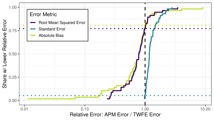
Figure 5.1: Plots of CDFs of error metric ratios between our estimator and the TWFE-based estimator across masked target parameters. The vertical, black, dashed line denotes the threshold above which our estimator performs worse than the TWFE estimator with respect to a given error metric, while the horizontal dotted lines correspond to the shares of target parameters for which our estimator performs better than the TWFE estimator on the error metric corresponding to its color, as labeled in the plot’s legend.

We illustrate the distributions of our estimation error metrics across target cohorts $c^{*}$ and outcomes $t^{*}$ in Figure 5.1. In particular, Figure 5.1 plots the cumulative distribution functions (CDF) of error metric ratios between our estimator and the TWFE-based estimator across masked target parameters. For over 75% of target cohorts and outcomes, our factor-model-based method attains smaller root mean squared error than the TWFE-based estimator. This frequent better performance is due to our estimator having lower bias than the TWFE-based estimator for over 80% of target cohorts and outcomes. The price of using our estimator over a TWFE-based estimator tends to be slightly higher variance, as indicated by the fact that the TWFE-based estimator had lower variance for over 90% of the target cohorts and outcomes we considered. However, the increased variance of our estimator is not enough to outweigh our estimator’s smaller bias relative to a TWFE-based estimator when comparing the root mean squared errors of the two methods, as discussed above. In Figure E.2, we provide scatter plots illustrating the estimators’ absolute error metric values and error metric values relative to the values of the target cohort outcome means across target cohorts and outcomes. Overall, this semi-synthetic simulation study provides more evidence that accounting for complementarities between workers and firms using a method like ours can yield more accurate estimates of average counterfactual match outcomes in bipartite matching settings.

6 Conclusion

In this paper, we develop a new approach for identifying and estimating average counterfactual outcomes with short panel data applicable in settings like event studies and studies of bipartite match outcomes. Relying only on an eigendecomposition of a new spectral operator, our method produces consistent, asymptotically normal estimates of means of outcomes generated by a latent factor model under general outcome missingness patterns as only the cross-sectional dimension of a panel grows large. Importantly, our procedure accommodates more general missingness patterns than other approaches for short panels, and it automatically stitches together different pieces of identifying information each used in isolation by existing methods. Through our simulation study based on the Veneto Worker Histories dataset, we also demonstrate the practicality of our approach in real-world “short” panel data settings.

Appendix A Proofs of Results in the Main Text

A.1 Proof of Lemma 4.1

By Assumption 4.2, there must exist at least one other cohort $c^{\prime}$ that is a neighbor of cohort $c$ in the observed outcome overlap graph $\mathcal{G}_{r}$. Further, since $E_{c^{\prime}}$ is a square matrix, the column space of $\Gamma^{\prime}E_{c}E_{c^{\prime}}$ must be a subset of the column space of $\Gamma^{\prime}E_{c}$, which, along with (4.1), implies that

$$\mathrm{rank}(\underbrace{E_{c}\Gamma}_{T\times r}) =\mathrm{rank}(\Gamma^{\prime}E_{c}) T>r$$ (, rank is min. of row rank and column rank) (A.1)

$$\geq\mathrm{rank}(\Gamma^{\prime}E_{c}E_{c^{\prime}})$$ (A.2)

$$=r \text{($c$ and $c^{\prime}$ are neighbors, so \eqref{cond:observed_outcome_overlap_graph_edge_def} holds)}.$$ (A.3)

Since $E_{c}\Gamma$ is $T\times r$ with $T>r$, $\mathrm{rank}(E_{c}\Gamma)\leq r$ must also hold, completing the proof.

A.2 Proof of Theorem 4.2

First, as in Footnote 15, we show that for any cohort $c$, the columns of $\Gamma$ lie in the null space of $E_{c}-\Pi(E_{c}\Gamma)$, in which case $\mathrm{col}(\Gamma)\subseteq\mathrm{null}(A)$, where $\mathrm{col}(\Gamma)$ denotes the column space of $\Gamma$. Since $E_{c}^{2}=E_{c}$ and $E_{c}\Pi(E_{c}\Gamma)=\Pi(E_{c}\Gamma)E_{c}=\Pi(E_{c}\Gamma)$, we have that

$$(E_{c}-\Pi(E_{c}\Gamma))\Gamma=(E_{c}^{2}-E_{c}\Pi(E_{c}\Gamma)E_{c})\Gamma=E_{c}\cdot(I-\Pi(E_{c}\Gamma))E_{c}\Gamma=\operatorname{\mathbf{0}}_{T\times r},$$ (A.4)

as required.

Next, we show that $\mathrm{null}(A)\subseteq\mathrm{col}(\Gamma)$ also holds. Define the matrix

$$\tilde{A}\coloneqq\begin{bmatrix}E_{1}-\Pi(E_{1}\Gamma)\\ \vdots\\ E_{C}-\Pi(E_{C}\Gamma)\end{bmatrix},$$ (A.5)

and note that since

$$(E_{c}-\Pi(E_{c}\Gamma))^{2}=E_{c}^{2}-E_{c}\Pi(E_{c}\Gamma)-\Pi(E_{c}\Gamma)E_{c}-\Pi(E_{c}\Gamma)^{2}=E_{c}-\Pi(E_{c}\Gamma)$$ (A.6)

and $E_{c}-\Pi(E_{c}\Gamma)$ is symmetric, $A=\tilde{A}^{\prime}\tilde{A}$, implying that $\mathrm{null}(A)=\mathrm{null}(\tilde{A})$.

Consider any $v\in\mathrm{null}(\tilde{A})$; by definition, it must be that for any cohort $c$, $(E_{c}-\Pi(E_{c}\Gamma))v=\operatorname{\mathbf{0}}_{T}$, which in turn implies that $E_{c}v\in\mathrm{col}(E_{c}\Gamma)$. Thus, there exists a vector $\omega_{c}\in\operatorname{\mathbb{R}}^{r}$ such that $E_{c}v=E_{c}\Gamma\omega_{c}$. Then, for any edge $(c_{1},c_{2})$ in the observed outcome overlap graph $\mathcal{G}_{r}$, since diagonal matrices commute,

$$E_{c_{1}}E_{c_{2}}v=E_{c_{2}}E_{c_{1}}v=E_{c_{2}}E_{c_{1}}\Gamma\omega_{c_{1}}=E_{c_{1}}E_{c_{2}}\Gamma\omega_{c_{1}},\quad E_{c_{1}}E_{c_{2}}v=E_{c_{1}}E_{c_{2}}\Gamma\omega_{c_{2}},$$ (A.7)

implying that $E_{c_{1}}E_{c_{2}}\Gamma(\omega_{c_{1}}-\omega_{c_{2}})=\operatorname{\mathbf{0}}_{T}$. Since (4.1) implies that the null space of $E_{c_{1}}E_{c_{2}}\Gamma$ is trivial and $\omega_{c_{1}}-\omega_{c_{2}}$ lies in it, $\omega_{c_{1}}=\omega_{c_{2}}$ must also hold. Since $\mathcal{G}_{r}$ is connected, there exists a path in $\mathcal{G}_{r}$ between any two cohorts, so $\omega_{1}=\dotsc=\omega_{C}=\omega$ for some common vector $\omega\in\operatorname{\mathbb{R}}^{r}$. For the $t$-th entry $v_{t}$ of $v$, since every outcome is observed for at least one cohort, there exists at least one cohort $c_{t}$ for whom $t\in\mathcal{T}_{c_{t}}$. Letting $e_{t}$ denote the $t$-th standard basis vector, we have that

$$v_{t}=e_{t}^{\prime}E_{c_{t}}\Gamma\omega=\gamma_{t}^{\prime}\omega,$$ (A.8)

which, stacking across $t=1,\dotsc,T$, implies that $v=\Gamma\omega$, i.e. $v\in\mathrm{col}(\Gamma)$. Putting everything together, we have that $\mathrm{null}(A)=\mathrm{null}(\tilde{A})\subseteq\mathrm{col}(\Gamma)$, as required.

A.3 Proof of Corollary 4.3

First, we show that Assumption 4.2 is sufficient to ensure that $E_{c^{*}}\tilde{\Gamma}$ is has full rank $r$ (since $T>r$ by assumption), and thus the $r\times r$ matrix $\tilde{\Gamma}^{\prime}E_{c^{*}}\tilde{\Gamma}=\left(E_{c^{*}}\tilde{\Gamma}\right)^{\prime}\cdot E_{c^{*}}\tilde{\Gamma}$ is invertible. Since $\tilde{\Gamma}$ is a basis for column space of $\Gamma$ by Theorem 4.2, there exists some invertible basis matrix $Q\in\operatorname{\mathbb{R}}^{r\times r}$ for which $\tilde{\Gamma}Q^{\prime}=\Gamma$, so $\tilde{\Gamma}=\Gamma\left(Q^{\prime}\right)^{-1}$. Then

$$\mathrm{rank}(E_{c^{*}}\tilde{\Gamma}) =\mathrm{rank}\left(E_{c^{*}}\Gamma\left(Q^{\prime}\right)^{-1}\right)$$ (A.9)

$$=\mathrm{rank}(\underbrace{E_{c^{*}}\Gamma}_{T\times r}) \left(Q^{\prime}\right)^{-1}$$ ( is full-rank) (A.10)

$$=r.$$ (Lemma 4.1) (A.11)

Next, since for full rank matrices $M$ with more rows than columns, $M^{+}=(M^{\prime}M)^{-1}M^{\prime}$, we have that

$$\tilde{\Gamma}\left(E_{c^{*}}\tilde{\Gamma}\right)^{+}\operatorname{\mathbb{E}}[E_{c^{*}}Y_{i}~{}|~{}C_{i}=c^{*}] =\Gamma Q^{\prime}\cdot(Q\Gamma^{\prime}E_{c^{*}}\Gamma Q^{\prime})^{-1}Q\Gamma^{\prime}E_{c^{*}}\cdot\operatorname{\mathbb{E}}[E_{c^{*}}Y_{i}~{}|~{}C_{i}=c^{*}]$$ (A.12)

$$=\Gamma\cdot(\Gamma^{\prime}E_{c^{*}}\Gamma)^{-1}\Gamma^{\prime}E_{c^{*}}\Gamma\operatorname{\mathbb{E}}[\lambda_{i}~{}|~{}C_{i}=c^{*}]$$ (A.13)

$$=\Gamma\cdot\operatorname{\mathbb{E}}[\lambda_{i}~{}|~{}C_{i}=c^{*}]$$ (A.14)

$$=\mu_{c^{*}},$$ (A.15)

as required.

A.4 Proof of Theorem 4.4

First, we show that $\lVert\hat{A}-A\rVert_{\mathrm{op}}=O_{p}\left(N^{-1/2}\right)$:

$$\lVert\hat{A}-A\rVert_{\mathrm{op}} \leq\lVert\hat{A}-A\rVert_{F}$$ (Equivalence of matrix norms) (A.16)

$$=\lVert\mathrm{vec}(\hat{A}-A)\rVert_{2}$$ (A.17)

$$\leq\sum_{c=1}^{C}\lVert\mathrm{vec}(\Pi(\hat{\Gamma}_{c})-\Pi(E_{c}\Gamma))\rVert_{2}. \hat{A} A$$ (Definitions of and ) (A.18)

By Assumption 4.3, $\mathrm{vec}(\Pi(\hat{\Gamma}_{c})-\Pi(E_{c}\Gamma))=O_{p}\left(N^{-1/2}\right)$. Since $T=O(1)$, it must be that $C=O(1)$ and hence $\lVert\hat{A}-A\rVert_{\mathrm{op}}=O_{p}\left(N^{-1/2}\right)$ as well.

Next, let $\lambda_{j}$ be the $j$th smallest eigenvalue of the population APM $A$, and denote a generic eigendecomposition of $A$ as follows:

$$A=\sum_{j=1}^{T}\lambda_{j}\Pi(u_{j}),$$ (A.19)

where $u_{j}$ is an eigenvector corresponding to the $j$th eigenvalue $\lambda_{j}$, and $\Pi(u_{j})$ is the projection onto the span of $u_{j}$. We note that all of $A$’s eigenvalues must be non-negative.

Given this notation, we now apply Theorem B.1 with $M=A$, $\hat{M}=\hat{A}$ as defined in Section 3, $s=0$, and $r=r$. We also note that $\lambda_{j}=\lambda_{j}(A)$ using the notation defined in Appendix B. Since Theorem 4.2 implies that

$$0=\lambda_{1}=\dotsc=\lambda_{r}<\lambda_{r+1},$$ (A.20)

we have that $\Delta(A)=4^{-1}\lambda_{r+1}>0$, satisfying (B.4). Further, Theorem 4.2 implies that

$$\Pi(\Gamma)=\Pi(U_{1:r}(A)),$$ (A.21)

and we define $\hat{\Gamma}$ in Section 3 such that

$$\Pi(\hat{\Gamma})=\Pi(U_{1:r}(\hat{A})).$$ (A.22)

Then so long as

$$\lVert\hat{A}-A\rVert_{\mathrm{op}}\leq 4^{-1}\lambda_{r+1},$$ (A.23)

Theorem B.1 implies that

$$\Bigg{\lVert}\Pi(\hat{\Gamma})-\Pi(\Gamma)-\sum_{j=1}^{r}\sum_{k=r+1}^{T}\lambda_{k}^{-1}\left[\Pi(u_{j})(\hat{A}-A)\Pi(u_{k})+\Pi(u_{k})(\hat{A}-A)\Pi(u_{j})\right]\Bigg{\rVert}_{\mathrm{op}}$$ (A.24)

$$\leq\frac{32}{\pi\lambda_{r+1}^{2}}\lVert\hat{A}-A\rVert_{\mathrm{op}}^{2}.$$

The fact that $\lVert\hat{A}-A\rVert_{\mathrm{op}}=O_{p}\left(N^{-1/2}\right)$ implies (A.23) holds with probability approaching one as $N\rightarrow\infty$, so by (A.24) and the definitions of $\hat{A}$ and $A$,

$$\Pi(\hat{\Gamma})-\Pi(\Gamma)$$ (A.25)

$$=\sum_{j=r+1}^{T}\frac{1}{\lambda_{j}}\sum_{k=1}^{r}\bigg{\{}\Pi(u_{j})(\hat{A}-A)\Pi(u_{k})+\Pi(u_{k})(\hat{A}-A)\Pi(u_{j})\bigg{\}}+o_{p}\left(N^{-1/2}\right).$$ (A.26)

$$=\left(\sum_{j=r+1}^{T}\frac{1}{\lambda_{j}}\Pi(u_{j})\right)(\hat{A}-A)\left(\sum_{k=1}^{r}\Pi(u_{k})\right)$$ (A.27)

$$\phantom{=}+\left(\sum_{k=1}^{r}\Pi(u_{k})\right)(\hat{A}-A)\left(\sum_{j=r+1}^{T}\frac{1}{\lambda_{j}}\Pi(u_{j})\right)+o_{p}\left(N^{-1/2}\right).$$ (A.28)

Next, since $\lambda_{1}=\dotsc=\lambda_{r}=0$, it must be that

$$\sum_{j=r+1}^{T}\frac{1}{\lambda_{j}}\Pi(u_{j})=\sum_{j=1}^{T}\frac{\mathbbm{1}\{j>r\}}{\lambda_{j}}\Pi(u_{j})=A^{+},$$ (A.29)

and since $\mathrm{rank}(\Gamma)=r$ and $\mathrm{null}(A)=\mathrm{col}(\Gamma)$,

$$\sum_{k=1}^{r}\Pi(u_{k})=\Pi(\Gamma).$$ (A.30)

Substituting these two simplifications back into (A.28) and applying the definitions of $\hat{A}$ and $A$, we have

$$\Pi(\hat{\Gamma})-\Pi(\Gamma)$$ (A.31)

$$=\sum_{c=1}^{C}\left\{A^{+}[\Pi(\hat{\Gamma}_{c})-\Pi(E_{c}\Gamma)]\Pi(\Gamma)+\Pi(\Gamma)[\Pi(\hat{\Gamma}_{c})-\Pi(E_{c}\Gamma)]A^{+}\right\}+o_{p}\left(N^{-1/2}\right).$$

Next, we note that the so-called mixed product property of the Kronecker product implies that, for any matrices $A\in\operatorname{\mathbb{R}}^{d\times m}$, $B\in\operatorname{\mathbb{R}}^{m\times p}$, and $C\in\operatorname{\mathbb{R}}^{p\times q}$,

$$\mathrm{vec}(ABC)=(C^{\prime}\otimes A)\mathrm{vec}(B).$$ (A.32)

Applying this fact to the vectorization of $\sqrt{N}$ times both sides of (A.31), since any projection matrix $\Pi(\cdot)$ is symmetric, we can write the vectorization of our scaled and centered statistic $\sqrt{N}(\Pi(\hat{\Gamma})-\Pi(\Gamma))$ as follows:

$$\sqrt{N}\mathrm{vec}(\Pi(\hat{\Gamma})-\Pi(\Gamma))$$ (A.33)

$$=\left(A^{+}\otimes\Pi(\Gamma)+\Pi(\Gamma)\otimes A^{+}\right)\left(\sum_{c=1}^{C}\sqrt{N}\mathrm{vec}\left(\Pi(\hat{\Gamma}_{c^{*}})-\Pi(E_{c^{*}}\Gamma)\right)\right)+o_{p}\left(1\right).$$

Combining (A.33) and (4.4) yields (4.5), as required.

By the triangle inequality and the product property of Kronecker product spectra (P. Lancaster  Farahat, 1972),

$$\left\lVert H\right\rVert_{\mathrm{op}}\leq\left\lVert A^{+}\otimes\Pi(\Gamma)\right\rVert_{\mathrm{op}}+\left\lVert\Pi(\Gamma)\otimes A^{+}\right\rVert_{\mathrm{op}}=2\left\lVert A^{+}\right\rVert_{\mathrm{op}}\left\lVert\Pi(\Gamma)\right\rVert_{\mathrm{op}}=\frac{2}{\lambda_{r+1}}<\infty.$$

The zero mean and bounded squared norm properties of $H\sum_{c=1}^{C}\phi_{c}(C_{i},Y_{i})$ follow from Assumption 4.3 and the fact that the operator norm of $H$ is bounded.

A.5 Proof of Theorem 4.5

First, we show that with probability approaching one as $N\rightarrow\infty$, $\hat{\Gamma}^{\prime}E_{c^{*}}\hat{\Gamma}$ is invertible. To do so, we note that by Theorem 4.4, $\Pi(\hat{\Gamma})-\Pi(\Gamma)=o_{p}\left(1\right)$, so there must be a random, $r\times r$ invertible basis matrix $\hat{Q}$ such that $\hat{\Gamma}\hat{Q}^{\prime}=\Gamma+o_{p}\left(1\right)$; if not, then for all random, $r\times r$ invertible basis matrices $\hat{Q}$, $\Pi(\hat{\Gamma})=\Pi(\hat{\Gamma}\hat{Q}^{\prime})\neq\Pi(\Gamma)+o_{p}\left(1\right)$, which would be a violation of Theorem 4.4. Since Lemma 4.1 implies that that $\Gamma^{\prime}E_{c^{*}}\Gamma$ is invertible and $\hat{\Gamma}^{\prime}E_{c^{*}}\hat{\Gamma}=(\hat{Q})^{-1}\Gamma E_{c^{*}}\Gamma(\hat{Q}^{\prime})^{-1}+o_{p}\left(1\right)$, it must be that $\hat{\Gamma}^{\prime}E_{c^{*}}\hat{\Gamma}$ is invertible with probability approaching one as $N\rightarrow\infty$. As such, in the remainder of the proof below, we condition on the event that $\hat{\Gamma}^{\prime}E_{c^{*}}\hat{\Gamma}$ is invertible.

Next, let $B_{c^{*}}\coloneqq\Gamma(\Gamma^{\prime}E_{c^{*}}\Gamma)^{-1}\Gamma^{\prime}E_{c^{*}}$ and $\hat{B}_{c^{*}}\coloneqq\hat{\Gamma}(\hat{\Gamma}^{\prime}E_{c^{*}}\hat{\Gamma})^{-1}\hat{\Gamma}^{\prime}E_{c^{*}}$, and note that

$$\hat{\mu}_{c^{*}}-\mu_{c^{*}} =\hat{B}_{c^{*}}\hat{\operatorname{\mathbb{E}}}_{N}[E_{c^{*}}Y_{i}~{}|~{}C_{i}=c^{*}]-B_{c^{*}}\operatorname{\mathbb{E}}[E_{c^{*}}Y_{i}~{}|~{}C_{i}=c^{*}]$$ (A.34)

$$=(\hat{B}_{c^{*}}-B_{c^{*}})E_{c^{*}}\mu_{c^{*}}+B_{c^{*}}(\hat{\operatorname{\mathbb{E}}}_{N}-\operatorname{\mathbb{E}})[E_{c^{*}}Y_{i}~{}|~{}C_{i}=c^{*}]$$ (A.35)

$$\phantom{=}+(\hat{B}_{c^{*}}-B_{c^{*}})(\hat{\operatorname{\mathbb{E}}}_{N}-\operatorname{\mathbb{E}})[E_{c^{*}}Y_{i}~{}|~{}C_{i}=c^{*}].$$ (A.36)

To approximate the expression $\hat{B}_{c^{*}}-B_{c^{*}}$, we will rely on the following lemma, which we prove in Appendix C.1:

Lemma A.1.

For any two $T\times r$ matrices $\hat{\Gamma}$ and $\Gamma$ such that $E_{c^{*}}\hat{\Gamma}$ and $E_{c^{*}}\Gamma$ are full-rank, let $\hat{\Delta}_{\Gamma}\coloneqq\Pi(\hat{\Gamma})-\Pi(\Gamma)$. If $\lVert\hat{\Delta}_{\Gamma}\rVert_{\mathrm{op}}\leq 1/\left(2\lVert R_{c^{*}}\rVert_{\mathrm{op}}\right)$, then the following first-order approximation holds:

$$\left\lVert(\hat{B}_{c^{*}}-B_{c^{*}})-\left(2E_{c^{*}}\hat{\Delta}_{\Gamma}R_{c^{*}}^{\prime}+(I+R_{c^{*}})\hat{\Delta}_{\Gamma}(I-R_{c^{*}})^{\prime}\right)E_{c^{*}}\right\rVert_{\mathrm{op}}\leq b\lVert\hat{\Delta}_{\Gamma}\rVert_{\mathrm{op}}^{2},$$ (A.37)

where $b\coloneqq 12\left(1+\left\lVert R_{c^{*}}\right\rVert_{\mathrm{op}}\right)^{3}<\infty$.

Since $\lVert\hat{\Delta}_{\Gamma}\rVert_{\mathrm{op}}=O_{p}\left(N^{-1/2}\right)$, the probability that $\lVert\hat{\Delta}_{\Gamma}\rVert_{\mathrm{op}}\leq 1/\left(2\lVert R_{c^{*}}\rVert_{\mathrm{op}}\right)$ converges to one. For the rest of the proof we also condition on this event so that Lemma A.1 can be applied. Letting

$$\hat{F}_{c^{*}}\coloneqq\left[2E_{c^{*}}\hat{\Delta}_{\Gamma}R_{c^{*}}^{\prime}+(I+R_{c^{*}})\hat{\Delta}_{\Gamma}(I-R_{c^{*}})^{\prime}\right]E_{c^{*}}.$$ (A.38)

By Lemma A.1,

$$\lVert\hat{B}_{c^{*}}-B_{c^{*}}\rVert_{\mathrm{op}}\leq\left[2\left\lVert R_{c^{*}}\right\rVert_{\mathrm{op}}+(1+\left\lVert R_{c^{*}}\right\rVert_{\mathrm{op}})^{2}\right]\lVert\hat{\Delta}_{\Gamma}\rVert_{\mathrm{op}}+b\lVert\hat{\Delta}_{\Gamma}\rVert_{\mathrm{op}}^{2}\leq b\left(\lVert\hat{\Delta}_{\Gamma}\rVert_{\mathrm{op}}+\lVert\hat{\Delta}_{\Gamma}\rVert_{\mathrm{op}}^{2}\right).$$ (A.39)

Using the fact that $\hat{F}_{c^{*}}E_{c^{*}}=\hat{F}_{c^{*}}$, we can further expand (A.36) as follows:

$$\hat{\mu}_{c^{*}}-\mu_{c^{*}}$$ (A.40)

$$=\hat{F}_{c^{*}}\mu_{c^{*}}+B_{c^{*}}(\hat{\operatorname{\mathbb{E}}}_{N}-\operatorname{\mathbb{E}})[E_{c^{*}}Y_{i}~{}|~{}C_{i}=c^{*}]$$

$$\phantom{=}+(\hat{B}_{c^{*}}-B_{c^{*}}-\hat{F}_{c^{*}})E_{c^{*}}\mu_{c^{*}}+(\hat{B}_{c^{*}}-B_{c^{*}})(\hat{\operatorname{\mathbb{E}}}_{N}-\operatorname{\mathbb{E}})[E_{c^{*}}Y_{i}~{}|~{}C_{i}=c^{*}]$$

Rearranging the display above and taking the norm, we have that, again by Lemma A.1,

$$\left\lVert\left[\hat{\mu}_{c^{*}}-\mu_{c^{*}}\right]-\hat{F}_{c^{*}}\mu_{c^{*}}-B_{c^{*}}(\hat{\operatorname{\mathbb{E}}}_{N}-\operatorname{\mathbb{E}})[E_{c^{*}}Y_{i}~{}|~{}C_{i}=c^{*}]\right\rVert_{2}$$ (A.41)

$$\leq\lVert\hat{B}_{c^{*}}-B_{c^{*}}-\hat{F}_{c^{*}}\rVert_{\mathrm{op}}\left\lVert E_{c^{*}}\mu_{c^{*}}\right\rVert_{2}$$

$$\phantom{=}+\lVert\hat{B}_{c^{*}}-B_{c^{*}}\rVert_{\mathrm{op}}\lVert(\hat{\operatorname{\mathbb{E}}}_{N}-\operatorname{\mathbb{E}})[E_{c^{*}}Y_{i}~{}|~{}C_{i}=c^{*}]\rVert_{2}$$

$$\leq b\lVert\hat{\Delta}_{\Gamma}\rVert_{\mathrm{op}}^{2}\left\lVert E_{c^{*}}\mu_{c^{*}}\right\rVert_{2}+b\left(\lVert\hat{\Delta}_{\Gamma}\rVert_{\mathrm{op}}+\lVert\hat{\Delta}_{\Gamma}\rVert_{\mathrm{op}}^{2}\right)\lVert(\hat{\operatorname{\mathbb{E}}}_{N}-\operatorname{\mathbb{E}})[E_{c^{*}}Y_{i}~{}|~{}C_{i}=c^{*}]\rVert_{2}.$$

Under Assumption 4.3, Theorem 4.4 implies that $\lVert\hat{\Delta}_{\Gamma}\rVert_{\mathrm{op}}=O_{p}\left(N^{-1/2}\right)$, and under Assumption 4.4,

$$\lVert(\hat{\operatorname{\mathbb{E}}}_{N}-\operatorname{\mathbb{E}})[E_{c^{*}}Y_{i}~{}|~{}C_{i}=c^{*}]\rVert_{2}\leq\lVert(\hat{\operatorname{\mathbb{E}}}_{N}-\operatorname{\mathbb{E}})[Y_{i}^{*}~{}|~{}C_{i}=c^{*}]\rVert_{2}=O_{p}\left(N^{-1/2}\right).$$ (A.42)

Therefore, by (A.41),

$$\sqrt{N}(\hat{\mu}_{c^{*}}-\mu_{c^{*}}) =\sqrt{N}\hat{F}_{c^{*}}\mu_{c^{*}}+\sqrt{N}B_{c^{*}}(\hat{\operatorname{\mathbb{E}}}_{N}-\operatorname{\mathbb{E}})[E_{c^{*}}Y_{i}~{}|~{}C_{i}=c^{*}]+o_{p}\left(1\right).$$ (A.43)

Applying (A.32) to the first term in the expansion (A.43), we have that

$$\sqrt{N}\hat{F}_{c^{*}}\mu_{c^{*}}$$ (A.44)

$$=\left((2\mu_{c^{*}}^{\prime}E_{c^{*}}R_{c^{*}})\otimes E_{c^{*}}+(\mu_{c^{*}}^{\prime}E_{c^{*}}(I-R_{c^{*}}))\otimes(I+R_{c^{*}})\right)\cdot\sqrt{N}\mathrm{vec}(\Pi(\hat{\Gamma})-\Pi(\Gamma))$$ (A.45)

$$=M_{c^{*}}\cdot\sqrt{N}\mathrm{vec}(\Pi(\hat{\Gamma})-\Pi(\Gamma))$$ (A.46)

$$=\sqrt{N}\hat{\operatorname{\mathbb{E}}}_{N}\left[M_{c^{*}}H\sum_{c=1}^{C}\phi_{c}(C_{i},Y_{i})\right]+o_{p}\left(1\right).$$ (A.47)

The following lemma, which we prove in Appendix C.2, will help us complete the proof:

Lemma A.2.

Let $V_{1},V_{2},\dotsc$ be a sequence of i.i.d. random variables such that $\operatorname{\mathbb{E}}[\lVert V_{1}\rVert_{2}^{2}]<\infty$, and let $D_{i}$ be a binary random variable such that $\operatorname{\mathbb{P}}(D_{i}=1)>0$. Then

$$\sqrt{N}\hat{\operatorname{\mathbb{E}}}_{N}[V_{i}~{}|~{}D_{i}=1]-\operatorname{\mathbb{E}}[V_{i}~{}|~{}D_{i}=1]=\sqrt{N}\hat{\operatorname{\mathbb{E}}}_{N}\left[\frac{D_{i}}{\operatorname{\mathbb{P}}(D_{i}=1)}\left(V_{i}-\operatorname{\mathbb{E}}[V_{i}~{}|~{}D_{i}=1]\right)\right]+o_{p}\left(1\right).$$ (A.48)

By Lemma A.2, we have that

$$(\hat{\operatorname{\mathbb{E}}}_{N}-\operatorname{\mathbb{E}})[E_{c^{*}}Y_{i}~{}|~{}C_{i}=c^{*}]=\hat{\operatorname{\mathbb{E}}}_{N}\left[\frac{\mathbbm{1}\{C_{i}=c^{*}\}}{\operatorname{\mathbb{P}}(C_{i}=c^{*})}\left(E_{c^{*}}Y_{i}-E_{c^{*}}\mu_{c^{*}}\right)\right].$$ (A.49)

Substituting the expressions in the two displays above back into (A.43) yields the asymptotically linear expansion in (4.7). Further, under (4.4) and (4.4), $\operatorname{\mathbb{E}}[\psi_{c^{*}}(C_{i},Y_{i})]=\operatorname{\mathbf{0}}_{T}$ and

$$\operatorname{\mathbb{E}}[\left\lVert\psi_{c^{*}i}\right\rVert_{2}^{2}]\leq\left\lVert M_{c^{*}}\right\rVert_{\mathrm{op}}^{2}\left\lVert H\right\rVert_{\mathrm{op}}^{2}\sum_{c=1}^{C}\operatorname{\mathbb{E}}[\left\lVert\phi_{c}(C_{i},Y_{i})\right\rVert_{2}^{2}]+2\operatorname{\mathbb{E}}\left[\lVert Y_{i}^{*}\rVert_{2}^{2}~{}\middle|~{}C_{i}=c^{*}\right]<\infty.$$ (A.50)

Appendix B An Exact, First-Order Expansion of the Eigenspace Operator on Symmetric Matrices

In this section, we derive an exact, first-order expansion of the operator mapping a symmetric matrix into the projection matrix onto the space spanned by some subset of its eigenvectors. Our expansion is based on Kato’s integral, which characterizes the projection matrix onto the space spanned by some subset of a matrix’s eigenvectors as a contour integral of that matrix’s resolvent Kato (1949). We characterize the approximation error in our expansion up to exact constants, unlike the asymptotic expansions given in e.g. Kato (1980) and Jg. Sun (1991) (which is applied in Simons (2023) to construct hypothesis tests concerning eigenspaces). As such, our result below may be of independent interest.

To describe our expansion, we first introduce some notation. Let $\mathbb{S}^{d}$ denote the set of real-valued, $d$-dimensional symmetric matrices, and for any $M\in\mathbb{S}^{d}$, let $\lambda_{j}(M)$ be the $j$th eigenvalue of $A$, where

$$\lambda_{0}(M)\coloneqq-\infty<\lambda_{1}(M)\leq\cdots\leq\lambda_{d}(M)<\lambda_{d+1}(M)\coloneqq\infty,$$ (B.1)

and we denote a generic eigendecomposition of $M$ as follows:

$$M=U(M)\Lambda(M)U(M)^{\prime}=\sum_{j=1}^{d}\lambda_{j}(M)\Pi(u_{j}(M)),$$ (B.2)

where $U(M)$ is any matrix with $j$th column $u_{j}(M)$ being an eigenvector corresponding to the $j$th eigenvalue $\lambda_{j}(M)$, and $\Pi(u_{j}(M))$ is the projection onto the span of $u_{j}(M)$. For notational convenience, for any integers $1\leq j,k\leq d$, we let

$$U_{j:k}(M)\coloneqq\begin{bmatrix}u_{j}(M)&\cdots&u_{k}(M)\end{bmatrix}$$ (B.3)

denote the matrix whose columns are the eigenvectors corresponding to the $j$th through $k$th eigenvalues.

Armed with this notation, we state our main result. In particular, we construct an exact bound on the error incurred by a first-order expansion of the difference between the projection matrices onto eigenspaces of two matrices $M$ and $\hat{M}$ in terms of the magnitude of the difference between $M$ and $\hat{M}$:

Theorem B.1.

Consider any integers $s,r$ such that $1\leq s+1\leq s+r\leq d$ and any real-valued, $d$-dimensional symmetric matrix $M$ satisfying the following eigen-gap condition:

$$\Delta(M)>0,\quad\Delta(M)\coloneqq 4^{-1}\min\left\{\lambda_{s+1}(M)-\lambda_{s}(M),\lambda_{s+r+1}(M)-\lambda_{s+r}(M)\right\},$$ (B.4)

and define the following neighborhood of $M$:

$$\mathcal{B}(M)\coloneqq\left\{\hat{M}\in\mathbb{S}^{d}~{}\operatorname{:}~{}\lVert\hat{M}-M\rVert_{\mathrm{op}}\leq\Delta(M)\right\}.$$ (B.5)

Then for any $\hat{M}\in\mathcal{B}(M)$, the following first-order approximation holds:

$$\Bigg{\lVert}\left[\Pi(U_{(s+1):(s+r)}(\hat{M}))-\Pi(U_{(s+1):(s+r)}(M))\right]$$ (B.6)

$$\phantom{\big{\lVert}}-\sum_{j=s+1}^{s+r}\sum_{k\not\in[s+1,s+r]}\frac{1}{\lambda_{k}(M)-\lambda_{j}(M)}\Big{[}\Pi(u_{j}(M))(\hat{M}-M)\Pi(u_{k}(M))$$

$$\phantom{\big{\lVert}-\sum_{j=s+1}^{s+r}\sum_{k\not\in[s+1,s+r]}\frac{1}{\lambda_{k}(M)-\lambda_{j}(M)}\Big{[}}+\Pi(u_{k}(M))(\hat{M}-M)\Pi(u_{j}(M))\Big{]}\Bigg{\rVert}_{\text{op}}$$

$$\leq\frac{2}{\pi\Delta(M)^{2}}\lVert\hat{M}-M\rVert_{\text{op}}^{2}.$$

Proof.

Consider any $\hat{M}\in\mathcal{B}(M)$. By Weyl’s inequality (see e.g. Theorem 4.5.3 in Vershynin (2018)),

$$\max_{j}\lvert\lambda_{j}(M)-\lambda_{j}(\hat{M})\rvert\leq\lVert M-\hat{M}\rVert_{\text{op}}\leq\Delta(M).$$ (B.7)

Let

$$a(M)\coloneqq\begin{cases}\frac{\lambda_{s+1}(M)+\lambda_{s}(M)}{2},&s>0\\ \lambda_{1}(M)-2\Delta(M),&s=0\end{cases},\quad b(M)\coloneqq\begin{cases}\frac{\lambda_{s+r+1}(M)+\lambda_{s+r}(M)}{2},&s+r<d\\ \lambda_{d}(M)+2\Delta(M),&s+r=d\end{cases}.$$ (B.8)

When $s>0$, it must be that

$$a(M)-\lambda_{s}(\hat{M})=\underbrace{\frac{\lambda_{s+1}(M)-\lambda_{s}(M)}{2}}_{\geq 2\Delta(M)}+\underbrace{\lambda_{s}(M)-\lambda_{s}(\hat{M})}_{\geq-\Delta(M)\text{ by \eqref{eq:eigval_diff_A_B_bound}}}\geq\Delta(M),$$ (B.9)

and

$$\lambda_{s+1}(\hat{M})-a(M)=\underbrace{\lambda_{s+1}(\hat{M})-\lambda_{s+1}(M)}_{\geq-\Delta(M)\text{ by \eqref{eq:eigval_diff_A_B_bound}}}+\underbrace{\frac{\lambda_{s+1}(M)-\lambda_{s}(M)}{2}}_{\geq 2\Delta(M)}\geq\Delta(M).$$ (B.10)

When $s=0$,

$$a(M)-\lambda_{s}(\hat{M})=\infty\geq\Delta(M),$$ (B.11)

and

$$\lambda_{s+1}(\hat{M})-a(M)=\underbrace{\lambda_{1}(\hat{M})-\lambda_{1}(M)}_{\geq-\Delta(M)\text{ by \eqref{eq:eigval_diff_A_B_bound}}}+2\Delta(M)\geq\Delta(M).$$ (B.12)

Thus, in both cases, by the definition of $\Delta(M)$ in (B.4),

$$\min\Bigg{\{} a(M)-\max\{\lambda_{s}(M),\lambda_{s}(\hat{M})\},\min\{\lambda_{s+1}(M),\lambda_{s+1}(\hat{M})\}-a(M)\Bigg{\}}\geq\Delta(M)>0.$$ (B.13)

Using similar logic, we can also show that

$$\min\Bigg{\{} b(M)-\max\{\lambda_{s+r}(M),\lambda_{s+r}(\hat{M})\},$$ (B.14)

$$\min\{\lambda_{s+r+1}(M),\lambda_{s+r+1}(\hat{M})\}-b(M)\Bigg{\}}\geq\Delta(M)>0.$$

Next, let $\mathcal{C}$ be some closed, bounded, positively oriented curve in $\mathbb{C}$ that intersects the real line only at $(\lambda_{s+1}(M)+\lambda_{s}(M))/2$ and $(\lambda_{s+r}(M)+\lambda_{s+r+1}(M))/2$. By (B.13) and (B.14), we have that the $(s+1)$th through $(s+r)$th eigenvalues of both $M$ and $\hat{M}$ are strictly inside $\mathcal{C}$, while all other eigenvalues are strictly outside $\mathcal{C}$. Problem I-5.9 in Kato (1980) (a result first shown in Kato (1949)) then dictates that for $\tilde{M}\in\{M,\hat{M}\}$,

$$\Pi(U_{(s+1):(s+r)}(\tilde{M}))=-\frac{1}{2\pi\sqrt{-1}}\oint_{\mathcal{C}}\left(\tilde{M}-\zeta I_{d}\right)^{-1}d\zeta,$$ (B.15)

so

$$\Pi(U_{(s+1):(s+r)}(\hat{M}))-\Pi(U_{(s+1):(s+r)}(M))$$ (B.16)

$$=\frac{1}{2\pi\sqrt{-1}}\oint_{\mathcal{C}}\left[\left(M-\zeta I_{d}\right)^{-1}-\left(\hat{M}-\zeta I_{d}\right)^{-1}\right]d\zeta.$$

Considering the integrand in (B.16) in more detail, we can apply the following lemma, which we prove in Appendix C.3:

Lemma B.2.

For any two invertible matrices $M,\hat{M}\in\operatorname{\mathbb{R}}^{d\times d}$, we have that

$$M^{-1}-\hat{M}^{-1}=M^{-1}(\hat{M}-M)M^{-1}-M^{-1}(\hat{M}-M)M^{-1}(\hat{M}-M)\hat{M}^{-1}.$$ (B.17)

Then

$$\left(M-\zeta I_{d}\right)^{-1}-\left(\hat{M}-\zeta I_{d}\right)^{-1}$$ (B.18)

$$=\left(M-\zeta I_{d}\right)^{-1}(\hat{M}-M)\left(M-\zeta I_{d}\right)^{-1}$$

$$\phantom{=}-\left(M-\zeta I_{d}\right)^{-1}(\hat{M}-M)\left(M-\zeta I_{d}\right)^{-1}(\hat{M}-M)\left(\hat{M}-\zeta I_{d}\right)^{-1}.$$

Returning to the expression (B.16), expanding the integrand via (B.18), rearranging terms, and taking the operator norm, we have that

$$\bigg{\lVert}\Pi(U_{(s+1):(s+r)}(\hat{M}))-\Pi(U_{(s+1):(s+r)}(M))$$ (B.19)

$$\phantom{\big{\lVert}}-\frac{1}{2\pi\sqrt{-1}}\oint_{\mathcal{C}}\left(M-\zeta I_{d}\right)^{-1}(\hat{M}-M)\left(M-\zeta I_{d}\right)^{-1}d\zeta\bigg{\rVert}_{\text{op}}$$

$$=\left\lVert\frac{1}{2\pi\sqrt{-1}}\oint_{\mathcal{C}}\left(M-\zeta I_{d}\right)^{-1}(\hat{M}-M)\left(M-\zeta I_{d}\right)^{-1}(\hat{M}-M)\left(\hat{M}-\zeta I_{d}\right)^{-1}d\zeta\right\rVert_{\text{op}}.$$

Take $\mathcal{C}$ to be the boundary of a positively oriented rectangular contour on the complex plane with the following corners for some $\upsilon>0$:

$$a(M)\pm\upsilon\sqrt{-1},\quad b(M)\pm\upsilon\sqrt{-1}.$$ (B.20)

Then we can bound the operator norm of the integral in (B.19) along each side of $\mathcal{C}$ separately.

To do so, for any $z\in\mathbb{C}$, we define the following decomposition of $z$ into its real and imaginary parts: $z=\mathrm{re}(z)+\mathrm{im}(z)\sqrt{-1}$. We then state the following convenient lemma, which we prove in Appendix C.4:

Lemma B.3.

For any real, symmetric matrix $B$,

$$\left\lVert\left(B-\zeta I_{d}\right)^{-1}\right\rVert_{\text{op}}=\max_{j}\left(\left(\lambda_{j}(B)-\mathrm{re}(\zeta)\right)^{2}+\mathrm{im}(\zeta)^{2}\right)^{-1/2}.$$ (B.21)

For notational convenience, we write $a$ and $b$ for $a(M)$ and $b(M)$, respectively. On the horizontal segment $\{x+v\sqrt{-1}:x\in[a,b]\}$,

$$\bigg{\|}\frac{1}{2\pi\sqrt{-1}}\int_{a}^{b}\left(M-(x+v\sqrt{-1})I_{d}\right)^{-1}(\hat{M}-M)\left(M-(x+v\sqrt{-1})I_{d}\right)^{-1}$$ (B.22)

$$\phantom{\bigg{\|}\frac{1}{2\pi\sqrt{-1}}\int_{a}^{b}}\cdot(\hat{M}-M)\left(\hat{M}-(x+v\sqrt{-1})I_{d}\right)^{-1}dx\bigg{\|}_{\text{op}}$$ (B.23)

$$\leq\frac{\lVert\hat{M}-M\rVert_{\text{op}}^{2}}{2\pi}\cdot\int_{a}^{b}\left\lVert\left(M-(x+v\sqrt{-1})I_{d}\right)^{-1}\right\rVert_{\text{op}}^{2}\left\lVert\left(\hat{M}-(x+v\sqrt{-1})I_{d}\right)^{-1}\right\rVert_{\text{op}}dx$$ (B.24)

$$\leq\frac{\lVert\hat{M}-M\rVert_{\text{op}}^{2}}{2\pi}\cdot\int_{a}^{b}\underbrace{\left((\lambda_{j}(M)-x)^{2}+v^{2}\right)^{-1}}_{\leq v^{-2}}\underbrace{\left((\lambda_{j}(\hat{M})-x)^{2}+v^{2}\right)^{-1/2}}_{\leq v^{-1}}dx$$ (by Lemma B.3) (B.25)

$$\leq\frac{\lVert\hat{M}-M\rVert_{\text{op}}^{2}}{2\pi}\cdot\frac{b-a}{v^{3}}.$$ (B.26)

Similarly, on the horizontal segment $\{x-v\sqrt{-1}:x\in[a,b]\}$,

$$\bigg{\|}\frac{1}{2\pi\sqrt{-1}}\int_{b}^{a}\left(M-(x-v\sqrt{-1})I_{d}\right)^{-1}(\hat{M}-M)\left(M-(x-v\sqrt{-1})I_{d}\right)^{-1}$$ (B.27)

$$\phantom{\bigg{\|}\frac{1}{2\pi\sqrt{-1}}\int_{b}^{a}}\cdot(\hat{M}-M)\left(\hat{M}-(x-v\sqrt{-1})I_{d}\right)^{-1}dx\bigg{\|}_{\text{op}}$$ (B.28)

$$\leq\frac{\lVert\hat{M}-M\rVert_{\text{op}}^{2}}{2\pi}\cdot\frac{b-a}{v^{3}}.$$ (B.29)

Now we turn to the vertical segment $\{a+y\sqrt{-1}:y\in[-v,v]\}$. By (B.13) and (B.14),

$$\lvert\lambda_{j}(M)-a\rvert \geq\min\Big{\{}\lvert\lambda_{s}(M)-a\rvert,\lvert\lambda_{s+1}(M)-a\rvert\Big{\}}\geq\Delta(M),$$ (B.30)

so by Lemma B.3,

$$\left\lVert\left(M-(a+y\sqrt{-1}))I_{d}\right)^{-1}\right\rVert_{\text{op}}=\max_{j}\left((\lambda_{j}(M)-a)^{2}+y^{2}\right)^{-1/2}\leq\left(\Delta(M)^{2}+y^{2}\right)^{-1/2}.$$ (B.31)

Since (B.13) and (B.14) also imply the bound $\lvert\lambda_{j}(\hat{M})-a\rvert\geq\Delta(M)$, Lemma B.3 also implies

$$\left\lVert\left(\hat{M}-(a+y\sqrt{-1}))I_{d}\right)^{-1}\right\rVert_{\text{op}}=\max_{j}\left((\lambda_{j}(\hat{M})-a)^{2}+y^{2}\right)^{-1/2}\leq\left(\Delta(M)^{2}+y^{2}\right)^{-1/2}.$$ (B.32)

Then, we can upper bound the operator norm of the integral on the vertical segment as follows:

$$\bigg{\|}\frac{1}{2\pi\sqrt{-1}}\int_{-v}^{v}\left(M-(a+y\sqrt{-1})I_{d}\right)^{-1}(\hat{M}-M)\left(M-(a+y\sqrt{-1})I_{d}\right)^{-1}$$ (B.33)

$$\phantom{\bigg{\|}\frac{1}{2\pi\sqrt{-1}}\int_{-v}^{v}}\cdot(\hat{M}-M)\left(\hat{M}-(a+y\sqrt{-1})I_{d}\right)^{-1}dx\bigg{\|}_{\text{op}}$$ (B.34)

$$\leq\frac{\lVert\hat{M}-M\rVert_{\text{op}}^{2}}{2\pi}\int_{-v}^{v}\left(\Delta(M)^{2}+y^{2}\right)^{-3/2}dy$$ (B.35)

$$\leq\frac{\lVert\hat{M}-M\rVert_{\text{op}}^{2}}{2\pi}\int_{-\infty}^{\infty}\left(\Delta(M)^{2}+y^{2}\right)^{-3/2}dy$$ (B.36)

$$=\frac{\lVert\hat{M}-M\rVert_{\text{op}}^{2}}{2\pi}\frac{1}{\Delta(M)^{2}}\int_{-\infty}^{\infty}\left(1+u^{2}\right)^{-3/2}du$$ (B.37)

$$=\frac{\lVert\hat{M}-M\rVert_{\text{op}}^{2}}{\pi}\cdot\frac{1}{\Delta(M)^{2}},$$ (B.38)

where the last line applies the following identity:

$$\int_{-\infty}^{\infty}\left(1+u^{2}\right)^{-3/2}du=\int_{-\pi/2}^{\pi/2}\left(1+\tan^{2}\theta\right)^{-3/2}d\tan\theta=\int_{-\pi/2}^{\pi/2}\cos\theta d\theta=\sin\pi/2-\sin(-\pi/2)=2.$$

Similarly, on the vertical segment $\{b+y\sqrt{-1}:y\in[-v,v]\}$,

$$\bigg{\|}\frac{1}{2\pi\sqrt{-1}}\int_{-v}^{v}\left(M-(b+y\sqrt{-1})I_{d}\right)^{-1}(\hat{M}-M)\left(M-(b+y\sqrt{-1})I_{d}\right)^{-1}$$ (B.39)

$$\phantom{\bigg{\|}\frac{1}{2\pi\sqrt{-1}}\int_{-v}^{v}}\cdot(\hat{M}-M)\left(\hat{M}-(b+y\sqrt{-1})I_{d}\right)^{-1}dx\bigg{\|}_{\text{op}}$$ (B.40)

$$\leq\frac{\lVert\hat{M}-M\rVert_{\text{op}}^{2}}{\pi}\cdot\frac{1}{\Delta(M)^{2}}.$$ (B.41)

Combining (B.26), (B.29), (B.38), and (B.41), we obtain that

$$\left\lVert\frac{1}{2\pi\sqrt{-1}}\oint_{\mathcal{C}}\left(M-\zeta I_{d}\right)^{-1}(\hat{M}-M)\left(M-\zeta I_{d}\right)^{-1}(\hat{M}-M)\left(\hat{M}-\zeta I_{d}\right)^{-1}d\zeta\right\rVert_{\text{op}}$$ (B.42)

$$\leq\frac{\lVert\hat{M}-M\rVert_{\text{op}}^{2}}{\pi}\left\{\frac{b-a}{v^{3}}+\frac{2}{\Delta(M)^{2}}\right\}.$$ (B.43)

Taking $v\rightarrow\infty$, we can combine the bound in the above display with (B.19) to obtain the following bound:

$$\bigg{\lVert}\Pi(U_{(s+1):(s+r)}(\hat{M}))-\Pi(U_{(s+1):(s+r)}(M))$$ (B.44)

$$\phantom{\big{\lVert}}-\frac{1}{2\pi\sqrt{-1}}\oint_{\mathcal{C}}\left(M-\zeta I_{d}\right)^{-1}(\hat{M}-M)\left(M-\zeta I_{d}\right)^{-1}d\zeta\bigg{\rVert}_{\text{op}}$$

$$\leq\frac{2\lVert\hat{M}-M\rVert_{\text{op}}^{2}}{\pi\Delta(M)^{2}}.$$

Next, we consider the first-order error term inside the operator norm in (B.44):

$$\frac{1}{2\pi\sqrt{-1}}\oint_{\mathcal{C}}\left(M-\zeta I_{d}\right)^{-1}(\hat{M}-M)\left(M-\zeta I_{d}\right)^{-1}d\zeta$$ (B.45)

$$=\frac{1}{2\pi\sqrt{-1}}\oint_{\mathcal{C}}U(M)(\Lambda(M)-\zeta I_{d})^{-1}U(M)^{\prime}(\hat{M}-M)U(M)(\Lambda(M)-\zeta I_{d})^{-1}U(M)^{\prime}d\zeta$$ (B.46)

$$=\frac{1}{2\pi\sqrt{-1}}\oint_{\mathcal{C}}\left[\sum_{j=1}^{d}(\lambda_{j}(M)-\zeta)^{-1}\Pi(u_{j}(M))\right](\hat{M}-M)\left[\sum_{j=1}^{d}(\lambda_{j}(M)-\zeta)^{-1}\Pi(u_{j}(M))\right]d\zeta$$ (B.47)

$$=\frac{1}{2\pi\sqrt{-1}}\sum_{j=1}^{d}\sum_{k=1}^{d}\Pi(u_{j}(M))(\hat{M}-M)\Pi(u_{k}(M))\oint_{\mathcal{C}}(\lambda_{j}(M)-\zeta)^{-1}(\lambda_{k}(M)-\zeta)^{-1}d\zeta.$$ (B.48)

When $j=k$, by Cauchy’s integral formula,

$$\oint_{\mathcal{C}}(\lambda_{j}(M)-\zeta)^{-1}(\lambda_{k}(M)-\zeta)^{-1}d\zeta=\oint_{\mathcal{C}}\frac{1}{(\lambda_{j}(M)-\zeta)^{2}}d\zeta=0,$$ (B.49)

and when $j\neq k$, we have that

$$\oint_{\mathcal{C}}(\lambda_{j}(M)-\zeta)^{-1}(\lambda_{k}(M)-\zeta)^{-1}d\zeta$$ (B.50)

$$=(\lambda_{j}(M)-\lambda_{k}(M))^{-1}$$ (B.51)

$$\phantom{=}\cdot\left(\oint_{\mathcal{C}}(\lambda_{k}(M)-\zeta)^{-1}d\zeta-\oint_{\mathcal{C}}(\lambda_{j}(M)-\zeta)^{-1}d\zeta\right)$$ (Partial Fraction Decomposition) (B.52)

$$=2\pi\sqrt{-1}(\lambda_{j}(M)-\lambda_{k}(M))^{-1}$$ (B.53)

$$\phantom{=}\cdot\left(\mathbbm{1}\{k\in[s+1,s+r]\}-\mathbbm{1}\{j\in[s+1,s+r]\}\right).$$ (Residue Theorem) (B.54)

Thus, we can rewrite (B.48) as follows:

$$\frac{1}{2\pi\sqrt{-1}}\oint_{\mathcal{C}}\left(M-\zeta I_{d}\right)^{-1}(\hat{M}-M)\left(M-\zeta I_{d}\right)^{-1}d\zeta$$ (B.55)

$$=\sum_{j=1}^{d}\sum_{k=1}^{d}\frac{\mathbbm{1}\{k\in[s+1,s+r]\}-\mathbbm{1}\{j\in[s+1,s+r]\}}{\lambda_{j}(M)-\lambda_{k}(M)}\Pi(u_{j}(M))(\hat{M}-M)\Pi(u_{k}(M))$$ (B.56)

$$=\sum_{j\not\in[s+1,s+r]}\sum_{k=s+1}^{s+r}\frac{1}{\lambda_{j}(M)-\lambda_{k}(M)}\Pi(u_{j}(M))(\hat{M}-M)\Pi(u_{k}(M))$$ (B.57)

$$\phantom{=}+\sum_{j=s+1}^{s+r}\sum_{k\not\in[s+1,s+r]}\frac{1}{\lambda_{k}(M)-\lambda_{j}(M)}\Pi(u_{j}(M))(\hat{M}-M)\Pi(u_{k}(M))$$ (B.58)

$$=\sum_{j=s+1}^{s+r}\sum_{k\not\in[s+1,s+r]}\frac{1}{\lambda_{k}(M)-\lambda_{j}(M)}\bigg{[}\Pi(u_{j}(M))(\hat{M}-M)\Pi(u_{k}(M))$$ (B.59)

$$\phantom{=\sum_{j=s+1}^{s+r}\sum_{k\not\in[s+1,s+r]}\frac{1}{\lambda_{k}(M)-\lambda_{j}(M)}\bigg{[}}+\Pi(u_{k}(M))(\hat{M}-M)\Pi(u_{j}(M))\bigg{]}.$$ (B.60)

Putting together (B.44) and the final expression in the display above yields (B.6). ∎

Appendix C Proofs of Intermediate Results

C.1 Proof of Lemma A.1

We begin by stating two helpful lemmas. The first lemma expresses our target quantity that is a function of the matrix $\Gamma$ as a function of $\Pi(\Gamma)$, which we prove in Appendix C.5:

Lemma C.1.

For any $T\times r$ matrix $\tilde{\Gamma}$ such that $E_{c^{*}}\tilde{\Gamma}$ is full-rank,

$$\tilde{\Gamma}\left(\tilde{\Gamma}^{\prime}E_{c^{*}}\tilde{\Gamma}\right)^{-1}\tilde{\Gamma}^{\prime}E_{c^{*}}=\left(I+E_{c^{*}}\Pi(\tilde{\Gamma})(1-E_{c^{*}})\right)G_{c^{*}}(\tilde{\Gamma})\Pi(\tilde{\Gamma})E_{c^{*}},$$ (C.1)

where

$$G_{c^{*}}(\tilde{\Gamma})\coloneqq(I-(I-E_{c^{*}})\Pi(\tilde{\Gamma})(I-E_{c^{*}}))^{-1}=I+(I-E_{c^{*}})\tilde{\Gamma}(\tilde{\Gamma}^{\prime}E_{c^{*}}\tilde{\Gamma})^{-1}\tilde{\Gamma}^{\prime}(I-E_{c^{*}})\eqqcolon I+D.$$ (C.2)

The second lemma states an expansion for $G_{c^{*}}(\hat{\Gamma})-G_{c^{*}}(\Gamma)$, which we prove in Appendix C.6.

Lemma C.2.

Suppose $E_{c^{*}}\Gamma$ and $E_{c^{*}}\hat{\Gamma}$ are both full-rank. Let $\hat{\Delta}_{G}=G_{c^{*}}(\hat{\Gamma})-G_{c^{*}}(\Gamma)$,and let $\ell_{c^{*}}=\|G_{c^{*}}(\Gamma)\|_{\mathrm{op}}$. If $\|\hat{\Delta}_{\Gamma}\|_{\mathrm{op}}\leq 1/2\ell_{c^{*}}$, then

$$\|\hat{\Delta}_{G}\|_{\mathrm{op}}\leq 2\ell_{c^{*}}^{2}\|\hat{\Delta}_{\Gamma}\|_{\mathrm{op}},$$ (C.3)

and

$$\|\hat{\Delta}_{G}+G_{c^{*}}(\Gamma)(I-E_{c^{*}})\hat{\Delta}_{\Gamma}(I-E_{c^{*}})G_{c^{*}}(\Gamma)\|_{\mathrm{op}}\leq 2\ell_{c^{*}}^{3}\|\hat{\Delta}_{\Gamma}\|_{\mathrm{op}}^{2}.$$ (C.4)

Now, we turn to the proof of Lemma A.1. First, by triangle inequality,

$$\ell_{c^{*}}\leq 1+\|R_{c^{*}}(I-E_{c^{*}})\|_{\mathrm{op}}\leq 1+\|R_{c^{*}}\|_{\mathrm{op}}.$$

Thus,

$$\|\hat{\Delta}_{\Gamma}\|_{\mathrm{op}}\leq 1/2\|R_{c^{*}}\|_{\mathrm{op}}\Longrightarrow\|\hat{\Delta}_{\Gamma}\|_{\mathrm{op}}\leq 1/2\ell_{c^{*}}.$$

Note that since $E_{c^{*}}\Gamma$ and $E_{c^{*}}\hat{\Gamma}$ are both full-rank, $G_{c^{*}}(\Gamma)$ and $G_{c^{*}}(\hat{\Gamma})$ are well-defined. Then

$$G_{c^{*}}(\hat{\Gamma})\Pi(\hat{\Gamma})-G_{c^{*}}(\Gamma)\Pi(\Gamma)=G_{c^{*}}(\Gamma)\hat{\Delta}_{\Gamma}+\hat{\Delta}_{G}\Pi(\Gamma)+\hat{\Delta}_{G}\hat{\Delta}_{\Gamma}.$$ (C.5)

Note that $G_{c^{*}}(\Gamma)\succeq I$ implies $\ell_{c^{*}}\geq 1$. By Lemma C.2,

$$\|G_{c^{*}}(\hat{\Gamma})\Pi(\hat{\Gamma})-G_{c^{*}}(\Gamma)\Pi(\Gamma)\|_{\mathrm{op}}$$ (C.6)

$$\leq\ell_{c^{*}}\|\hat{\Delta}_{\Gamma}\|_{\mathrm{op}}+\|\hat{\Delta}_{G}\|_{\mathrm{op}}\|\Pi(\Gamma)\|_{\mathrm{op}}+\|\hat{\Delta}_{G}\|_{\mathrm{op}}\|\hat{\Delta}_{\Gamma}\|_{\mathrm{op}}$$ (C.7)

$$\leq(\ell_{c^{*}}+2\ell_{c^{*}}^{2}+2\ell_{c^{*}}^{2}\|\hat{\Delta}_{\Gamma}\|_{\mathrm{op}})\|\hat{\Delta}_{\Gamma}\|_{\mathrm{op}})$$ (by (C.3)) (C.8)

$$\leq 2\ell_{c^{*}}(1+\ell_{c^{*}})\|\hat{\Delta}_{\Gamma}\|_{\mathrm{op}}$$ (C.9)

$$\leq 4\ell_{c^{*}}^{2}\|\hat{\Delta}_{\Gamma}\|_{\mathrm{op}},$$ (C.10)

and

$$\bigg{\|}G_{c^{*}}(\hat{\Gamma})\Pi(\hat{\Gamma})-G_{c^{*}}(\Gamma)\Pi(\Gamma)$$ (C.11)

$$\phantom{\bigg{\|}}-\left(G_{c^{*}}(\Gamma)\hat{\Delta}_{\Gamma}-G_{c^{*}}(\Gamma)(I-E_{c^{*}})\hat{\Delta}_{\Gamma}(I-E_{c^{*}})G_{c^{*}}(\Gamma)\Pi(\Gamma)\right)\bigg{\|}_{\text{op}}$$ (C.12)

$$\leq\|\hat{\Delta}_{G}\|_{\mathrm{op}}\|\hat{\Delta}_{\Gamma}\|_{\mathrm{op}}+2\ell_{c^{*}}^{3}\|\hat{\Delta}_{\Gamma}\|_{\mathrm{op}}^{2}\|\Pi(\Gamma)\|_{\mathrm{op}}$$ (by (C.4)) (C.13)

$$\leq 2\ell_{c^{*}}^{2}(1+\ell_{c^{*}})\|\hat{\Delta}_{\Gamma}\|_{\mathrm{op}}^{2}$$ (by (C.3)) (C.14)

$$\leq 4\ell_{c^{*}}^{3}\|\hat{\Delta}_{\Gamma}\|_{\mathrm{op}}^{2}.$$ (C.15)

By Lemma C.1,

$$\hat{\Delta}_{B} \coloneqq\hat{\Gamma}(\hat{\Gamma}^{\prime}E_{c^{*}}\hat{\Gamma})^{-1}\hat{\Gamma}^{\prime}E_{c^{*}}-\Gamma(\Gamma^{\prime}E_{c^{*}}\Gamma)^{-1}\Gamma^{\prime}E_{c^{*}}$$ (C.16)

$$=E_{c^{*}}\hat{\Delta}_{\Gamma}(I-E_{c^{*}})G_{c^{*}}(\Gamma)\Pi(\Gamma)E_{c^{*}}$$ (C.17)

$$\quad+\left(I+E_{c^{*}}\Pi(\Gamma)(1-E_{c^{*}})\right)(G_{c^{*}}(\hat{\Gamma})\Pi(\hat{\Gamma})-G_{c^{*}}(\Gamma)\Pi(\Gamma))E_{c^{*}}$$ (C.18)

$$\quad+E_{c^{*}}\hat{\Delta}_{\Gamma}(I-E_{c^{*}})G_{c^{*}}(\Gamma)(G_{c^{*}}(\hat{\Gamma})\Pi(\hat{\Gamma})-G_{c^{*}}(\Gamma)\Pi(\Gamma))E_{c^{*}}.$$ (C.19)

By (C.15), we can approximate the second term of (C.19) as follows:

$$\Bigg{\|}\left(I+E_{c^{*}}\Pi(\Gamma)(1-E_{c^{*}})\right)(G_{c^{*}}(\hat{\Gamma})\Pi(\hat{\Gamma})-G_{c^{*}}(\Gamma)\Pi(\Gamma))E_{c^{*}}$$ (C.20)

$$-\left(I+E_{c^{*}}\Pi(\Gamma)(1-E_{c^{*}})\right)\left(G_{c^{*}}(\Gamma)\hat{\Delta}_{\Gamma}-G_{c^{*}}(\Gamma)(I-E_{c^{*}})\hat{\Delta}_{\Gamma}(I-E_{c^{*}})G_{c^{*}}(\Gamma)\Pi(\Gamma)\right)E_{c^{*}}\Bigg{\|}_{\mathrm{op}}$$ (C.21)

$$\leq\|I+E_{c^{*}}\Pi(\Gamma)(1-E_{c^{*}})\|_{\mathrm{op}}\|E_{c^{*}}\|_{\mathrm{op}}\cdot 4\ell_{c^{*}}^{3}\|\hat{\Delta}_{\Gamma}\|_{\mathrm{op}}^{2}$$ (C.22)

$$\leq 8\ell_{c^{*}}^{3}\|\hat{\Delta}_{\Gamma}\|_{\mathrm{op}}^{2}.$$ (C.23)

By (C.10), we can bound the third term of (C.19) as follows:

$$\|E_{c^{*}}\hat{\Delta}_{\Gamma}(I-E_{c^{*}})G_{c^{*}}(\Gamma)(G_{c^{*}}(\hat{\Gamma})\Pi(\hat{\Gamma})-G_{c^{*}}(\Gamma)\Pi(\Gamma))E_{c^{*}}\|_{\mathrm{op}}$$ (C.24)

$$\leq\|\hat{\Delta}_{\Gamma}\|_{\mathrm{op}}\cdot\ell_{c^{*}}\cdot 4\ell_{c^{*}}^{2}\|\hat{\Delta}_{\Gamma}\|_{\mathrm{op}}=4\ell_{c^{*}}^{3}\|\hat{\Delta}_{\Gamma}\|_{\mathrm{op}}^{2}.$$ (C.25)

Putting together (C.19), (C.23), and (C.25), we obtain that

$$\Bigg{\|}\hat{\Delta}_{B}-\Bigg{(}E_{c^{*}}\hat{\Delta}_{\Gamma}(I-E_{c^{*}})G_{c^{*}}(\Gamma)\Pi(\Gamma)E_{c^{*}}$$ (C.26)

$$+\left(I+E_{c^{*}}\Pi(\Gamma)(1-E_{c^{*}})\right)G_{c^{*}}(\Gamma)\left(\hat{\Delta}_{\Gamma}-(I-E_{c^{*}})\hat{\Delta}_{\Gamma}(I-E_{c^{*}})G_{c^{*}}(\Gamma)\Pi(\Gamma)\right)E_{c^{*}}\Bigg{)}\Bigg{\|}_{\mathrm{op}}$$ (C.27)

$$\leq 12\ell_{c^{*}}^{3}\|\hat{\Delta}_{\Gamma}\|_{\mathrm{op}}^{2}.$$ (C.28)

By (C.2),

$$G_{c^{*}}(\Gamma)E_{c^{*}}=(I+D)E_{c^{*}}=E_{c^{*}}.$$

Thus,

$$G_{c^{*}}(\Gamma)(I-E_{c^{*}}) =(I-E_{c^{*}})G_{c^{*}}(\Gamma)=G_{c^{*}}(\Gamma)-E_{c^{*}},$$ (C.29)

$$(I-E_{c^{*}})G_{c^{*}}(\Gamma)(I-E_{c^{*}}) =(I-E_{c^{*}})G_{c^{*}}(\Gamma).$$

Let

$$K_{c^{*}}(\Gamma) \coloneqq G_{c^{*}}(\Gamma)(I-E_{c^{*}})\Pi(\Gamma)E_{c^{*}}=(I-E_{c^{*}})G_{c^{*}}(\Gamma)\Pi(\Gamma)E_{c^{*}}$$ (C.30)

$$=(I-E_{c^{*}})G_{c^{*}}(\Gamma)(I-E_{c^{*}})\Pi(\Gamma)E_{c^{*}}.$$ (C.31)

Then the left-hand side of (C.28) simplifies to

$$\Bigg{\|}\hat{\Delta}_{B}-\Bigg{(}E_{c^{*}}\hat{\Delta}_{\Gamma}K_{c^{*}}(\Gamma)+(G_{c^{*}}(\Gamma)+K_{c^{*}}^{\prime})\hat{\Delta}_{\Gamma}E_{c^{*}}$$ (C.32)

$$-\left(I+E_{c^{*}}\Pi(\Gamma)(1-E_{c^{*}})\right)(I-E_{c^{*}})G_{c^{*}}(\Gamma)\hat{\Delta}_{\Gamma}(I-E_{c^{*}})G_{c^{*}}(\Gamma)\Pi(\Gamma)E_{c^{*}}\Bigg{)}\Bigg{\|}_{\mathrm{op}}$$ (C.33)

$$=\Bigg{\|}\hat{\Delta}_{B}-\Bigg{(}E_{c^{*}}\hat{\Delta}_{\Gamma}K_{c^{*}}(\Gamma)+(G_{c^{*}}(\Gamma)+K_{c^{*}}(\Gamma)^{\prime})\hat{\Delta}_{\Gamma}E_{c^{*}}-\left((I-E_{c^{*}})G_{c^{*}}(\Gamma)+K_{c^{*}}(\Gamma)^{\prime}\right)\hat{\Delta}_{\Gamma}K_{c^{*}}(\Gamma)\Bigg{)}\Bigg{\|}_{\mathrm{op}}$$ (C.34)

$$=\Bigg{\|}\hat{\Delta}_{B}-\Bigg{(}E_{c^{*}}\hat{\Delta}_{\Gamma}K_{c^{*}}(\Gamma)+(G_{c^{*}}(\Gamma)+K_{c^{*}}(\Gamma)^{\prime})\hat{\Delta}_{\Gamma}E_{c^{*}}-\left(G_{c^{*}}(\Gamma)-E_{c^{*}}+K_{c^{*}}(\Gamma)^{\prime}\right)\hat{\Delta}_{\Gamma}K_{c^{*}}(\Gamma)\Bigg{)}\Bigg{\|}_{\mathrm{op}}$$ (C.35)

$$=\Bigg{\|}\hat{\Delta}_{B}-\Bigg{(}2E_{c^{*}}\hat{\Delta}_{\Gamma}K_{c^{*}}(\Gamma)+(G_{c^{*}}(\Gamma)+K_{c^{*}}(\Gamma)^{\prime})\hat{\Delta}_{\Gamma}(E_{c^{*}}-K_{c^{*}}(\Gamma))\Bigg{)}\Bigg{\|}_{\mathrm{op}}.$$ (C.36)

By (C.65) and (C.73),

$$K_{c^{*}}(\Gamma)=(I-E_{c^{*}})\Gamma(\Gamma^{\prime}E_{c^{*}}\Gamma)^{-1}\Gamma^{\prime}E_{c^{*}}=R_{c^{*}}^{\prime}E_{c^{*}}.$$

By (C.61) and (C.73),

$$G_{c^{*}}(\Gamma)=I+(I-E_{c^{*}})\Gamma(\Gamma^{\prime}E_{c^{*}}\Gamma)^{-1}\Gamma^{\prime}(I-E_{c^{*}})=I+(I-E_{c^{*}})R_{c^{*}}.$$

Thus,

$$G_{c^{*}}(\Gamma)+K_{c^{*}}(\Gamma)^{\prime}=I+R_{c^{*}}.$$

Plugging the expression in the display above into (C.36) completes the proof.

C.2 Proof of Lemma A.2

First, note that $\hat{\operatorname{\mathbb{E}}}_{N}[D_{i}V_{i}]=\operatorname{\mathbb{E}}[D_{i}V_{i}]+O_{p}\left(N^{-1/2}\right)$ and $\hat{\operatorname{\mathbb{E}}}_{N}[D_{i}]=\operatorname{\mathbb{P}}(D_{i}=1)+O_{p}\left(N^{-1/2}\right)$ by a classical multivariate Central Limit Theorem. Then

$$\hat{\operatorname{\mathbb{E}}}_{N}[V_{i}~{}|~{}D_{i}=1]-\operatorname{\mathbb{E}}[V_{i}~{}|~{}D_{i}=1]$$ (C.37)

$$=\frac{1}{\hat{\operatorname{\mathbb{E}}}_{N}[D_{i}]}\hat{\operatorname{\mathbb{E}}}_{N}[D_{i}V_{i}]-\operatorname{\mathbb{E}}[V_{i}~{}|~{}D_{i}=1]$$ (C.38)

$$=\left(\frac{1}{\hat{\operatorname{\mathbb{E}}}_{N}[D_{i}]}-\frac{1}{\operatorname{\mathbb{P}}(D_{i}=1)}\right)\hat{\operatorname{\mathbb{E}}}_{N}[D_{i}V_{i}]+\frac{1}{\operatorname{\mathbb{P}}(D_{i}=1)}\hat{\operatorname{\mathbb{E}}}_{N}[D_{i}V_{i}]-\operatorname{\mathbb{E}}[V_{i}~{}|~{}D_{i}=1]$$ (C.39)

$$=\frac{\operatorname{\mathbb{P}}(D_{i}=1)-\hat{\operatorname{\mathbb{E}}}_{N}[D_{i}]}{\hat{\operatorname{\mathbb{E}}}_{N}[D_{i}]\operatorname{\mathbb{P}}(D_{i}=1)}\hat{\operatorname{\mathbb{E}}}_{N}[D_{i}V_{i}]+\frac{1}{\operatorname{\mathbb{P}}(D_{i}=1)}\hat{\operatorname{\mathbb{E}}}_{N}[D_{i}V_{i}]-\operatorname{\mathbb{E}}[V_{i}~{}|~{}D_{i}=1]$$ (C.40)

$$=\frac{\operatorname{\mathbb{P}}(D_{i}=1)-\hat{\operatorname{\mathbb{E}}}_{N}[D_{i}]}{\operatorname{\mathbb{P}}(D_{i}=1)^{2}}\hat{\operatorname{\mathbb{E}}}_{N}[D_{i}V_{i}]+\frac{1}{\operatorname{\mathbb{P}}(D_{i}=1)}\hat{\operatorname{\mathbb{E}}}_{N}[D_{i}V_{i}]-\operatorname{\mathbb{E}}[V_{i}~{}|~{}D_{i}=1]$$ (C.41)

$$\phantom{=}+\left(\frac{\operatorname{\mathbb{P}}(D_{i}=1)-\hat{\operatorname{\mathbb{E}}}_{N}[D_{i}]}{\hat{\operatorname{\mathbb{E}}}_{N}[D_{i}]\operatorname{\mathbb{P}}(D_{i}=1)}-\frac{\operatorname{\mathbb{P}}(D_{i}=1)-\hat{\operatorname{\mathbb{E}}}_{N}[D_{i}]}{\operatorname{\mathbb{P}}(D_{i}=1)^{2}}\right)\hat{\operatorname{\mathbb{E}}}_{N}[D_{i}V_{i}]$$ (C.42)

$$=\frac{\operatorname{\mathbb{P}}(D_{i}=1)-\hat{\operatorname{\mathbb{E}}}_{N}[D_{i}]}{\operatorname{\mathbb{P}}(D_{i}=1)^{2}}\operatorname{\mathbb{E}}[D_{i}V_{i}]+\frac{1}{\operatorname{\mathbb{P}}(D_{i}=1)}\hat{\operatorname{\mathbb{E}}}_{N}[D_{i}V_{i}]-\operatorname{\mathbb{E}}[V_{i}~{}|~{}D_{i}=1]$$ (C.43)

$$\phantom{=}+\underbrace{\frac{\operatorname{\mathbb{P}}(D_{i}=1)-\hat{\operatorname{\mathbb{E}}}_{N}[D_{i}]}{\operatorname{\mathbb{P}}(D_{i}=1)^{2}}\left(\hat{\operatorname{\mathbb{E}}}_{N}[D_{i}V_{i}]-\operatorname{\mathbb{E}}[D_{i}V_{i}]\right)}_{O_{p}\left(N^{-1}\right)}$$ (C.44)

$$\phantom{=}+\left(\frac{1}{\hat{\operatorname{\mathbb{E}}}_{N}[D_{i}]\operatorname{\mathbb{P}}(D_{i}=1)}-\frac{1}{\operatorname{\mathbb{P}}(D_{i}=1)^{2}}\right)\left(\operatorname{\mathbb{P}}(D_{i}=1)-\hat{\operatorname{\mathbb{E}}}_{N}[D_{i}]\right)\hat{\operatorname{\mathbb{E}}}_{N}[D_{i}V_{i}]$$ (C.45)

$$=\hat{\operatorname{\mathbb{E}}}_{N}\left[\varphi(D_{i},V_{i})\right]+\underbrace{\left(\operatorname{\mathbb{P}}(D_{i}=1)-\hat{\operatorname{\mathbb{E}}}_{N}[D_{i}]\right)^{2}}_{O_{p}\left(N^{-1}\right)}\underbrace{\frac{1}{\hat{\operatorname{\mathbb{E}}}_{N}[D_{i}]\operatorname{\mathbb{P}}(D_{i}=1)^{2}}\hat{\operatorname{\mathbb{E}}}_{N}[D_{i}V_{i}]}_{O_{p}\left(1\right)}+o_{p}\left(N^{-1/2}\right).$$ (C.46)

Since

$$\operatorname{\mathbb{E}}\left[\varphi(D_{i},V_{i})\right] =\frac{1}{\operatorname{\mathbb{P}}(D_{i}=1)}\operatorname{\mathbb{E}}[D_{i}V_{i}]-\operatorname{\mathbb{E}}[V_{i}~{}|~{}D_{i}=1],$$ (C.47)

a classical multivariate Central Limit Theorem implies that

$$\sqrt{N}\hat{\operatorname{\mathbb{E}}}_{N}[V_{i}~{}|~{}D_{i}=1]-\operatorname{\mathbb{E}}[V_{i}~{}|~{}D_{i}=1]\stackrel{{\scriptstyle d}}{{\longrightarrow}}\mathcal{N}\left(\operatorname{\mathbf{0}},\operatorname{\mathbb{E}}\left[\varphi(D_{i},V_{i})\varphi(D_{i},V_{i})^{\prime}\right]\right),$$ (C.48)

and

$$\operatorname{\mathbb{E}}\left[\varphi(D_{i},V_{i})\varphi(D_{i},V_{i})^{\prime}\right] =\operatorname{\mathbb{E}}\left[\frac{D_{i}}{\operatorname{\mathbb{P}}(D_{i}=1)^{2}}\left(V_{i}-\operatorname{\mathbb{E}}[V_{i}~{}|~{}D_{i}=1]\right)\left(V_{i}-\operatorname{\mathbb{E}}[V_{i}~{}|~{}D_{i}=1]\right)^{\prime}\right]$$ (C.49)

$$=\frac{1}{\operatorname{\mathbb{P}}(D_{i}=1)}\operatorname{\mathbb{E}}\left[\left(V_{i}-\operatorname{\mathbb{E}}[V_{i}~{}|~{}D_{i}=1]\right)\left(V_{i}-\operatorname{\mathbb{E}}[V_{i}~{}|~{}D_{i}=1]\right)^{\prime}~{}\middle|~{}D_{i}=1\right]$$ (C.50)

$$=\frac{1}{\operatorname{\mathbb{P}}(D_{i}=1)}\operatorname{Var}(V_{i}~{}|~{}D_{i}=1),$$ (C.51)

as required.

C.3 Proof of Lemma B.2

$$M^{-1}-\hat{M}^{-1} =M^{-1}\hat{M}\hat{M}^{-1}-M^{-1}M\hat{M}^{-1}$$ (C.52)

$$=M^{-1}(\hat{M}-M)\hat{M}^{-1}$$ (C.53)

$$=M^{-1}(\hat{M}-M)\hat{M}^{-1}+M^{-1}(\hat{M}-M)M^{-1}-M^{-1}(\hat{M}-M)M^{-1}$$ (C.54)

$$=M^{-1}(\hat{M}-M)M^{-1}-M^{-1}(\hat{M}-M)\left(M^{-1}-\hat{M}^{-1}\right).$$ (C.55)

Applying (C.53) to the last expression in the display above yields the desired result.

C.4 Proof of Lemma B.3

Since $B$ is symmetric and real, $\lambda_{j}(B)$ must be real, in which case, letting $z^{*}$ denote the complex conjugate of $z\in\mathbb{C}$,

$$\left\lVert\left(B-\zeta I_{d}\right)^{-1}\right\rVert_{\text{op}} =\max_{j}\left((\lambda_{j}(B)-\zeta)^{*}(\lambda_{j}(B)-\zeta)\right)^{-1/2}$$ (C.56)

$$=\max_{j}\left(\left(\lambda_{j}(B)-\mathrm{re}(\zeta)-\mathrm{im}(\zeta)\sqrt{-1})\right)\left(\lambda_{j}(B)-\mathrm{re}(\zeta)+\mathrm{im}(\zeta)\sqrt{-1}\right)\right)^{-1/2}$$ (C.57)

$$=\max_{j}\left(\left(\lambda_{j}(B)-\mathrm{re}(\zeta)\right)^{2}-\mathrm{im}(\zeta)^{2}\cdot(-1)\right)^{-1/2},$$ (C.58)

which equals the desired result.

C.5 Proof of Lemma C.1

First, we note that for any matrix $\tilde{\Gamma}\in\operatorname{\mathbb{R}}^{T\times r}$, we can divide $\Pi(\tilde{\Gamma})$ up into four disjoint sets of entries via left (to select rows) and right (to select columns) multiplications by $E_{c^{*}}$ and $(I-E_{c^{*}})$ as follows:

$$\Pi(\tilde{\Gamma})=(E_{c^{*}}\tilde{\Gamma}+(I-E_{c^{*}})\tilde{\Gamma})\left(\tilde{\Gamma}^{\prime}E_{c^{*}}\tilde{\Gamma}+\tilde{\Gamma}^{\prime}(I-E_{c^{*}})\tilde{\Gamma}\right)^{-1}(E_{c^{*}}\tilde{\Gamma}+(I-E_{c^{*}})\tilde{\Gamma})^{\prime}.$$ (C.59)

Recall that for any invertible $M$, the Sherman-Morrison-Woodbury matrix identity states that

$$(M+C^{\prime}C)^{-1}=M^{-1}-M^{-1}C^{\prime}(I+CM^{-1}C^{\prime})^{-1}CM^{-1}.$$ (C.60)

Letting $M=\tilde{\Gamma}^{\prime}E_{c^{*}}\tilde{\Gamma},C=(I-E_{c^{*}})\tilde{\Gamma}$, we have that

$$\left(\tilde{\Gamma}^{\prime}E_{c^{*}}\tilde{\Gamma}+\tilde{\Gamma}^{\prime}(I-E_{c^{*}})\tilde{\Gamma}\right)^{-1}$$ (C.61)

$$=\left(\tilde{\Gamma}^{\prime}E_{c^{*}}\tilde{\Gamma}\right)^{-1}$$

$$\phantom{=}-\left(\tilde{\Gamma}^{\prime}E_{c^{*}}\tilde{\Gamma}\right)^{-1}\tilde{\Gamma}^{\prime}(I-E_{c^{*}})$$

$$\phantom{=-}\cdot\left(I+\underbrace{(I-E_{c^{*}})\tilde{\Gamma}\left(\tilde{\Gamma}^{\prime}E_{c^{*}}\tilde{\Gamma}\right)^{-1}\tilde{\Gamma}^{\prime}(I-E_{c^{*}})}_{D}\right)^{-1}(I-E_{c^{*}})\tilde{\Gamma}\left(\tilde{\Gamma}^{\prime}E_{c^{*}}\tilde{\Gamma}\right)^{-1}.$$

Then using (C.61) and (C.59), we can write an equation with our quantity of interest on one side:

$$E_{c^{*}}\Pi(\tilde{\Gamma})E_{c^{*}} =\tilde{\Gamma}\left(\tilde{\Gamma}^{\prime}E_{c^{*}}\tilde{\Gamma}\right)^{-1}\tilde{\Gamma}^{\prime}E_{c^{*}}$$ (C.62)

$$\phantom{=}-\underbrace{(I-E_{c^{*}})\tilde{\Gamma}\left(\tilde{\Gamma}^{\prime}E_{c^{*}}\tilde{\Gamma}\right)^{-1}\tilde{\Gamma}^{\prime}E_{c^{*}}}_{K}$$ (C.63)

$$\phantom{=}-E_{c^{*}}\tilde{\Gamma}\left(\tilde{\Gamma}^{\prime}E_{c^{*}}\tilde{\Gamma}\right)^{-1}\tilde{\Gamma}^{\prime}(I-E_{c^{*}})\left(I+D\right)^{-1}(I-E_{c^{*}})\tilde{\Gamma}\left(\tilde{\Gamma}^{\prime}E_{c^{*}}\tilde{\Gamma}\right)^{-1}\tilde{\Gamma}^{\prime}E_{c^{*}}$$ (C.64)

$$=\tilde{\Gamma}\left(\tilde{\Gamma}^{\prime}E_{c^{*}}\tilde{\Gamma}\right)^{-1}\tilde{\Gamma}^{\prime}E_{c^{*}}-K-K^{\prime}(I+D)^{-1}K.$$ (C.65)

Next, note that, again by (C.61) and (C.59),

$$(I-E_{c^{*}})\Pi(\tilde{\Gamma})(I-E_{c^{*}}) =D-D(I+D)^{-1}D$$ (C.66)

$$=(I+D)(I+D)^{-1}D-D(I+D)^{-1}D$$ (C.67)

$$=(I+D-D)(I+D)^{-1}D$$ (C.68)

$$=(I+D)^{-1}D$$ (C.69)

$$=(I+D)^{-1}(I+D-I)$$ (C.70)

$$=I-(I+D)^{-1},$$ (C.71)

and

$$E_{c^{*}}\Pi(\tilde{\Gamma})(I-E_{c^{*}})=K^{\prime}-K^{\prime}(I+D)^{-1}D=K^{\prime}(I-(I+D)^{-1}D)=K^{\prime}(I+D)^{-1}.$$ (C.72)

Therefore,

$$(I+D)^{-1} =I-(I-E_{c^{*}})\Pi(\tilde{\Gamma})(I-E_{c^{*}})=G_{c^{*}}(\tilde{\Gamma})^{-1},$$ (C.73)

$$K =(I+D)(I-E_{c^{*}})\Pi(\tilde{\Gamma})E_{c^{*}}$$

$$=\left(I-(I-E_{c^{*}})\Pi(\tilde{\Gamma})(I-E_{c^{*}})\right)^{-1}(I-E_{c^{*}})\Pi(\tilde{\Gamma})E_{c^{*}}$$

$$=G_{c^{*}}(\tilde{\Gamma})(I-E_{c^{*}})\Pi(\tilde{\Gamma})E_{c^{*}}.$$

Substituting (C.72) and the components of (C.73) into (C.65) and rearranging, we have that

$$\tilde{\Gamma}\left(\tilde{\Gamma}^{\prime}E_{c^{*}}\tilde{\Gamma}\right)^{-1}\tilde{\Gamma}^{\prime}E_{c^{*}}$$ (C.74)

$$=E_{c^{*}}\Pi(\tilde{\Gamma})E_{c^{*}}+G_{c^{*}}(\tilde{\Gamma})(I-E_{c^{*}})\Pi(\tilde{\Gamma})E_{c^{*}}+E_{c^{*}}\Pi(\tilde{\Gamma})(I-E_{c^{*}})G_{c^{*}}(\tilde{\Gamma})(I-E_{c^{*}})\Pi(\tilde{\Gamma})E_{c^{*}},$$ (C.75)

which simplifies to (C.1). By (C.29),

$$\tilde{\Gamma}\left(\tilde{\Gamma}^{\prime}E_{c^{*}}\tilde{\Gamma}\right)^{-1}\tilde{\Gamma}^{\prime}E_{c^{*}}$$ (C.76)

$$=E_{c^{*}}\Pi(\tilde{\Gamma})E_{c^{*}}+(G_{c^{*}}(\tilde{\Gamma})-E_{c^{*}})\Pi(\tilde{\Gamma})E_{c^{*}}+E_{c^{*}}\Pi(\tilde{\Gamma})(I-E_{c^{*}})G_{c^{*}}(\tilde{\Gamma})\Pi(\tilde{\Gamma})E_{c^{*}}$$ (C.77)

$$=\left(I+E_{c^{*}}\Pi(\tilde{\Gamma})(I-E_{c^{*}})\right)G_{c^{*}}(\tilde{\Gamma})\Pi(\tilde{\Gamma})E_{c^{*}}.$$ (C.78)

C.6 Proof of Lemma C.2

By (C.53),

$$\hat{\Delta}_{G}=-G_{c^{*}}(\Gamma)(I-E_{c^{*}})\hat{\Delta}_{\Gamma}(I-E_{c^{*}})G_{c^{*}}(\hat{\Gamma}).$$ (C.79)

Thus, since

$$\|G_{c^{*}}(\hat{\Gamma})\|_{\mathrm{op}}=\|G_{c^{*}}(\Gamma)+\hat{\Delta}_{G}\|_{\mathrm{op}}\leq\|G_{c^{*}}(\Gamma)\|_{\mathrm{op}}+\|\hat{\Delta}_{G}\|_{\mathrm{op}}\leq\ell_{c^{*}}+\|\hat{\Delta}_{G}\|_{\mathrm{op}},$$ (C.80)

we have that

$$\|\hat{\Delta}_{G}\|_{\mathrm{op}} \leq\|G_{c^{*}}(\Gamma)\|_{\mathrm{op}}\|G_{c^{*}}(\hat{\Gamma})\|_{\mathrm{op}}\|\hat{\Delta}_{\Gamma}\|_{\mathrm{op}}$$ (C.81)

$$\leq\ell_{c^{*}}(\ell_{c^{*}}+\|\hat{\Delta}_{G}\|_{\mathrm{op}})\|\hat{\Delta}_{\Gamma}\|_{\mathrm{op}}$$ (by (C.80)) (C.82)

$$\leq\ell_{c^{*}}^{2}\|\hat{\Delta}_{\Gamma}\|_{\mathrm{op}}+\frac{1}{2}\|\hat{\Delta}_{G}\|_{\mathrm{op}}.$$ (C.83)

where the last line uses the condition that $\|\hat{\Delta}_{\Gamma}\|_{\mathrm{op}}\leq 1/2\ell_{c^{*}}$. Rearranging the display above implies (C.3).

As a further consequence of this line of reasoning, we have that

$$\|G_{c^{*}}(\hat{\Gamma})\|_{\mathrm{op}} \leq\ell_{c^{*}}+\|\hat{\Delta}_{G}\|_{\mathrm{op}}$$ (by (C.80)) (C.84)

$$\leq\ell_{c^{*}}+2\ell_{c^{*}}^{2}\|\hat{\Delta}_{\Gamma}\|_{\mathrm{op}}$$ (by (C.3)) (C.85)

$$\leq 2\ell_{c^{*}}. \|\hat{\Delta}_{\Gamma}\|_{\mathrm{op}}\leq 1/2\ell_{c^{*}}$$ () (C.86)

Our desired result then follows from the following display:

$$\|\hat{\Delta}_{G}+G_{c^{*}}(\Gamma)(I-E_{c^{*}})\hat{\Delta}_{\Gamma}(I-E_{c^{*}})G_{c^{*}}(\Gamma)\|_{\mathrm{op}}$$ (C.87)

$$\leq\|G_{c^{*}}(\Gamma)(I-E_{c^{*}})\hat{\Delta}_{\Gamma}(I-E_{c^{*}})G_{c^{*}}(\Gamma)(I-E_{c^{*}})\hat{\Delta}_{\Gamma}(I-E_{c^{*}})G_{c^{*}}(\hat{\Gamma})\|_{\mathrm{op}}$$ (by Lemma B.2) (C.88)

$$\leq\ell_{c^{*}}^{2}\|G_{c^{*}}(\hat{\Gamma})\|_{\mathrm{op}}\|\hat{\Delta}_{\Gamma}\|_{\mathrm{op}}^{2} \|\hat{\Delta}_{\Gamma}\|_{\mathrm{op}}\leq 1/2\ell_{c^{*}}$$ () (C.89)

$$\leq 2\ell_{c^{*}}^{3}\|\hat{\Delta}_{\Gamma}\|_{\mathrm{op}}^{2}.$$ (by (C.86)) (C.90)

Appendix D Supplementary Discussions and Results

D.1 Target Parameters: Examples, Estimation, and Inference

In this appendix, we introduce two examples of target parameters $\theta=h(\mu,\eta)$ that aggregate cohort outcome means $\mu$ and nuisance parameters $\eta$ nonlinearly through $h$ as introduced in Section 3. We then establish that the plug-in estimator $\hat{\theta}$ described in Section 3 is a consistent and asymptotically normal estimator of $\theta$, and that the Bayesian-bootstrap-based simultaneous confidence intervals described in Section 3 have valid simultaneous coverage.

Example D.1 (Dynamic Treatment Effects).

In event study settings, researchers are often interested in reporting dynamic treatment effect paths, i.e. average effects of a treatment across different numbers of time periods relative to units’ treatment times. Recall that, in our notation, outcome $Y_{it}^{*}$ refers to unit $i$’s potential outcome in period $t$ had they not yet been treated by period $t$, $C_{i}$ refers to unit $i$’s first treatment period, and the set of observed outcomes for the units treated in period $c$ is $\mathcal{T}_{c}\subset\{1,\dotsc,c-1\}$. To express dynamic treatment effects in the form $h(\mu,\eta)$, we first define $Z_{it}^{*}$ as unit $i$’s potential outcome in period $t$ had they been treated in period $C_{i}$, and, to distinguish between observed and missing outcomes, we let $Z_{it}=Z_{it}^{*}$ if unit $i$ was treated by period $t$ (i.e. $C_{i}\leq t$) and $Z_{it}=\emptyset$ otherwise.

Assuming we observe either $Y_{it}^{*}$ or $Z_{it}^{*}$ in every period for simplicity, we can write dynamic treatment effect parameters from $b$ periods before treatment through $p-b$ periods after treatment in the form of Equation (3.4) in Callaway  Sant’Anna (2021) or Equation (26) in L. Sun  Abraham (2021):

$$\theta_{\text{dyn},j} \coloneqq\sum_{t=1}^{T}\sum_{c=1}^{C}\mathbbm{1}\{t-c=j-b+1\}\operatorname{\mathbb{P}}(C_{i}=c)$$ (D.1)

$$\phantom{\coloneqq\sum_{t=1}^{T}\sum_{c=1}^{C}}\cdot\left(\underbrace{\operatorname{\mathbb{E}}[\mathbbm{1}\{t\geq c\}Z_{it}+\mathbbm{1}\{t<c\}Y_{it}~{}|~{}C_{i}=c]}_{m_{ct}}-\mu_{ct}\right).$$

We note that $\theta_{\text{dyn},j}$ can be defined without any restrictions on heterogeneity in treatment effects $Z_{it}^{*}-Y_{it}^{*}$ across units or time periods (Callaway  Sant’Anna, 2021; L. Sun  Abraham, 2021).

Example D.2 (Match Outcome Attribution).

In the context of bipartite match outcomes, a common exercise is to attribute differences between the outcomes of row-type units matched to two different column-type units to either differences in how column-type units affect match outcomes on average across all row-type units or selection of different row-type units into matches with different column-type units. Analogous to Finkelstein . (2016), we note that the difference in average observed match outcomes for row-type units matched to column-type units $t_{1}$ and $t_{2}$ can be decomposed additively as follows:

$$\operatorname{\mathbb{E}}[Y_{it_{1}}~{}|~{}t_{1}\in\mathcal{T}_{C_{i}}]-\operatorname{\mathbb{E}}[Y_{it_{1}}~{}|~{}t_{2}\in\mathcal{T}_{C_{i}}]$$ (D.2)

$$=\underbrace{\operatorname{\mathbb{E}}[Y_{it_{1}}^{*}]-\operatorname{\mathbb{E}}[Y_{it_{2}}^{*}]}_{\text{Average effect of column-type unit differences on match outcomes}}$$

$$\phantom{=}+\underbrace{(\operatorname{\mathbb{E}}[Y_{it_{1}}^{*}~{}|~{}t_{1}\in\mathcal{T}_{C_{i}}]-\operatorname{\mathbb{E}}[Y_{it_{1}}^{*}])-(\operatorname{\mathbb{E}}[Y_{it_{2}}^{*}~{}|~{}t_{2}\in\mathcal{T}_{C_{i}}]-\operatorname{\mathbb{E}}[Y_{it_{2}}^{*}]).}_{\text{Average effect on outcomes of differential row-type unit selection into matches with column-type units $t_{1}$ and $t_{2}$}}$$

In line with Finkelstein . (2016), we can then define

$$\theta_{\text{col},t_{1},t_{2}}\coloneqq\frac{\operatorname{\mathbb{E}}[Y_{it_{1}}^{*}]-\operatorname{\mathbb{E}}[Y_{it_{2}}^{*}]}{\operatorname{\mathbb{E}}[Y_{it_{1}}~{}|~{}t_{1}\in\mathcal{T}_{C_{i}}]-\operatorname{\mathbb{E}}[Y_{it_{1}}~{}|~{}t_{2}\in\mathcal{T}_{C_{i}}]},$$ (D.3)

as the “share” of the difference in average observed match outcomes between column-type unit $t_{1}$ and column-type unit $t_{2}$ that can be attributed to differences in how column-type units $t_{1}$ and $t_{2}$ affect match outcomes on average across all units, and we can define

$$\theta_{\text{row},t_{1},t_{2}}\coloneqq\frac{(\operatorname{\mathbb{E}}[Y_{it_{1}}^{*}~{}|~{}t_{1}\in\mathcal{T}_{C_{i}}]-\operatorname{\mathbb{E}}[Y_{it_{1}}^{*}])-(\operatorname{\mathbb{E}}[Y_{it_{2}}^{*}~{}|~{}t_{2}\in\mathcal{T}_{C_{i}}]-\operatorname{\mathbb{E}}[Y_{it_{2}}^{*}])}{\operatorname{\mathbb{E}}[Y_{it_{1}}~{}|~{}t_{1}\in\mathcal{T}_{C_{i}}]-\operatorname{\mathbb{E}}[Y_{it_{1}}~{}|~{}t_{2}\in\mathcal{T}_{C_{i}}]}$$ (D.4)

as the “share” of the difference in average observed match outcomes between column-type unit $t_{1}$ and column-type unit $t_{2}$ that can be attributed to differences in which row-type units select into matches with column-type unit $t_{1}$ versus column-type unit $t_{2}$. We put “share” in quotes because, like in Finkelstein . (2016), $\theta_{\text{col}}$ and $\theta_{\text{row}}$ need not lie between zero and one.

We note that the definitions of $\theta_{\text{col},t_{1},t_{2}}$ and $\theta_{\text{row},t_{1},t_{2}}$ above are only defined in terms of outcomes, which is beneficial for interpretation (Hull, 2018), but they coincide exactly with $S_{\text{place}}$ and $S_{\text{pat}}$ in Finkelstein . (2016) when $Y_{it}^{*}$ is determined by the TWFE model $\operatorname{\mathbb{E}}[Y_{it}^{*}~{}|~{}\lambda_{i},C_{i}]=\lambda_{i}+\gamma_{t}$:

$$\theta_{\text{col},t_{1},t_{2}} \propto\gamma_{t_{1}}-\gamma_{t_{2}}$$ (D.5)

$$\theta_{\text{row},t_{1},t_{2}} \propto\operatorname{\mathbb{E}}[\lambda_{i}~{}|~{}t_{1}\in\mathcal{T}_{C_{i}}]-\operatorname{\mathbb{E}}[\lambda_{i}~{}|~{}t_{2}\in\mathcal{T}_{C_{i}}].$$

As discussed in Finkelstein . (2016), one could also extend this decomposition by studying analogous differences in average observed match outcomes across both units and groups of outcomes $\mathcal{T}\subset\{1,\dotsc,T\}$, i.e. differences in

$$\frac{1}{\lvert\mathcal{T}\rvert}\sum_{t\in\mathcal{T}}\operatorname{\mathbb{E}}[Y_{it}~{}|~{}t\in\mathcal{T}_{C_{i}}]$$ (D.6)

between two groups of column-type units $\mathcal{T}=\check{\mathcal{T}}$ and $\mathcal{T}=\tilde{\mathcal{T}}$. For simplicity however, we restrict our attention to $\theta_{\text{col},t_{1},t_{2}}$ and $\theta_{\text{row},t_{1},t_{2}}$ in our remaining discussion.

Having established in Section 4.2 that $\hat{\mu}_{c}$ is an asymptotically linear estimator of the vector of cohort outcome means $\mu_{c}$, we now establish asymptotic linearity of our plug-in estimator $\hat{\theta}$ of our target estimand $\theta=h(\mu,\eta)$ and validity of our simultaneous confidence intervals $\hat{\mathcal{C}}_{j}$. To do so, we assume that nuisance parameter estimator $\hat{\eta}$ is also asymptotically linear:

Assumption D.1.

There exists an additional observed random vector $\varrho_{i}\in\operatorname{\mathbb{R}}^{q}$ measurable with respect to the same probability space as $(C_{i},Y_{i}^{*})$ that satisfies $\operatorname{\mathbb{E}}[\varrho_{i}]=\operatorname{\mathbf{0}}_{q}$ and $\operatorname{\mathbb{E}}[\lVert\varrho_{i}\rVert_{2}^{2}]<\infty$ such that the following expansion holds as $N\rightarrow\infty$:

$$\sqrt{N}(\hat{\eta}-\eta)=\sqrt{N}\hat{\operatorname{\mathbb{E}}}_{N}\left[\varrho_{i}\right]+o_{p}\left(1\right).$$ (D.7)

In addition, we assume that the function $h$ that defines $\theta=h(\mu,\eta)$ is sufficiently smooth:

Assumption D.2.

$h\colon\operatorname{\mathbb{R}}^{CT}\times\operatorname{\mathbb{R}}^{q}\to\operatorname{\mathbb{R}}^{p}$ is differentiable at $(\mu,\eta)$.

Under the additional Assumptions D.1 and D.2, our desired result holds:

Corollary D.1.

Suppose that Assumptions 4.1, 4.2, 4.3, 4.4, D.1, and D.2 hold. Then

$$\sqrt{N}(\hat{\theta}-\theta) =\sqrt{N}\hat{\operatorname{\mathbb{E}}}_{N}\left[\varphi(C_{i},Y_{i},\varrho_{i})\right]+o_{p}\left(1\right),$$ (D.8)

$$\varphi(C_{i},Y_{i},\varrho_{i}) \coloneqq\sum_{c=1}^{C}\frac{\partial h}{\partial\mu_{c}^{\prime}}\psi_{c}(C_{i},Y_{i})+\frac{\partial h}{\partial\eta^{\prime}}\varrho_{i},$$

$\operatorname{\mathbb{E}}[\varphi(C_{i},Y_{i},\varrho_{i})]=\operatorname{\mathbf{0}}_{p}$, and $\operatorname{\mathbb{E}}[\lVert\varphi(C_{i},Y_{i},\varrho_{i})\rVert_{2}^{2}]<\infty$. Further, as $N\rightarrow\infty$,

$$\sqrt{N}(\hat{\theta}-\theta)\stackrel{{\scriptstyle d}}{{\longrightarrow}}\mathcal{N}\left(\operatorname{\mathbf{0}}_{p},\Sigma_{\theta}\right),\quad\Sigma_{\theta}\coloneqq\operatorname{\mathbb{E}}[\varphi(C_{i},Y_{i},\varrho_{i})\varphi(C_{i},Y_{i},\varrho_{i})^{\prime}].$$ (D.9)

Corollary D.1 follows from a straightforward application of the Delta Method and a classical multivariate Central Limit Theorem.

Before continuing, we note that $\Sigma_{\theta}$ is not guaranteed to be strictly positive definite. For example, if the target parameter $\theta=a^{\prime}\mu_{c^{*}}$ for some $T$-dimensional vector $a$ and target cohort $c^{*}$, and the target cohort’s average loadings $\operatorname{\mathbb{E}}[\lambda_{i}~{}|~{}C_{i}=c^{*}]=\operatorname{\mathbf{0}}_{r}$, then by (4.7) and (D.8), the asymptotic variance $\Sigma_{\theta}$ of $\hat{\theta}$ is given by the following quadratic form of at most rank $r$:

$$\Sigma_{\theta}=a^{\prime}\operatorname{Var}(\psi_{c^{*}}(C_{i},Y_{i}))a=a^{\prime}\underbrace{\Gamma}_{T\times r}\underbrace{\left(E_{c^{*}}\Gamma\right)^{+}\operatorname{Var}\left(E_{c^{*}}Y_{i}~{}|~{}C_{i}=c^{*}\right)\left(\left(E_{c^{*}}\Gamma\right)^{+}\right)^{\prime}}_{r\times r}\underbrace{\Gamma^{\prime}}_{r\times T}a.$$ (D.10)

Since the rank $r$ of $\operatorname{Var}(\psi_{c^{*}}(C_{i},Y_{i}))$ is smaller than its dimension $T$, there are non-zero vectors $a$ that lie in its non-trivial null space, and thus for those target parameters, $\hat{\theta}$ will have zero asymptotic variance. An implication of this limiting distribution degeneracy is that the confidence intervals $\hat{\mathcal{C}}_{j}$ defined in (3.5) based on the limiting Gaussian distribution (D.9) will have zero width for some coordinates and thus zero coverage of those coordinates. The following assumption rules out such knife-edge cases:

Assumption D.3.

The diagonal entries of $\Sigma_{\theta}$ are all strictly positive.

To state our result on the validity of our inference procedure under this assumption, we define the random vector $\hat{\theta}^{*}=\hat{\theta}(W)$, where $\hat{\theta}(\cdot)$ is defined in (3.2), $W$ is a random vector of weights with $i$th coordinate given by $W_{i}=\xi_{i}/\sum_{j=1}^{N}\xi_{j}$, and $\xi_{1},\dotsc,\xi_{N}$ are draws from $\mathrm{Exponential}(1)$ independent of both each other and $\hat{\theta}(\cdot)$. Then, under some slight generalizations of Assumptions 4.3 and D.1 stated in Appendix F.1 for brevity, our inference procedure satisfies the following validity guarantee:

Theorem D.2.

Suppose that Assumptions 4.1, 4.2, 4.4, D.2, and D.3 hold, along with Assumptions F.1 and F.2 stated in Appendix F.1. Then the confidence intervals $\hat{\mathcal{C}}_{j}$ for the coordinates of $\theta$ have asymptotic simultaneous coverage at least $1-\alpha$:

$$\liminf_{N\rightarrow\infty}\operatorname{\mathbb{P}}\left(\theta\in\bigtimes_{j=1}^{p}\hat{\mathcal{C}}_{j}\right)\geq 1-\alpha.$$ (D.11)

We provide a proof of Theorem D.2 in Appendix F.1.

We now return to Examples D.1 and D.2 and verify that Assumptions D.2 and F.2 (and therefore Assumption D.1) hold:

Example D.3 (continues=ex:dynamic_treatment_effects).

From (D.1), we can see that the cohort sizes $\operatorname{\mathbb{P}}(C_{i}=c)$ and cohort-specific observed outcome means $m_{ct}$ are not included in $\mu$ and thus form the components of $\eta$ we must also estimate. Of course, $\operatorname{\mathbb{P}}(C_{i}=c)$ and $m_{ct}$ are identified and consistently estimable via simple averages of the observables $\mathbbm{1}\{C_{i}=c\}$, $\mathbbm{1}\{t\geq C_{i}\}Z_{it}$, and $\mathbbm{1}\{t<C_{i}\}Y_{it}$. Thus, by standard arguments, the components of $\eta$ expressed as a map from distributions to nuisance parameter values (see Appendix F.1 for details) must be Hadamard differentiable with respect to the distribution over which the expectations in their definitions are taken, implying Assumption F.2 and, by extension, the weaker Assumption D.1 hold. Since $\theta_{\text{dyn},j}$ is linear in products of the components of $\mu$ and $\eta$, Assumption D.2 immediately holds as well.

Example D.4 (continues=ex:match_outcome_attribution).

To verify that our target parameters $\theta_{\text{col},t_{1},t_{2}}$ and $\theta_{\text{row},t_{1},t_{2}}$ satisfy the assumptions required for Theorem D.2 to hold, we first note that they are functions of $\operatorname{\mathbb{E}}[Y_{it}~{}|~{}t\in\mathcal{T}_{C_{i}}]$, which can be expressed as follows:

$$\operatorname{\mathbb{E}}[Y_{it}~{}|~{}t\in\mathcal{T}_{C_{i}}]=\frac{\operatorname{\mathbb{E}}[\mathbbm{1}\{t\in\mathcal{T}_{C_{i}}\}Y_{it}]}{\operatorname{\mathbb{E}}[\mathbbm{1}\{t\in\mathcal{T}_{C_{i}}\}]}=\frac{\sum_{c=1}^{C}\mathbbm{1}\{t\in\mathcal{T}_{c}\}\operatorname{\mathbb{P}}(C_{i}=c)\mu_{ct}}{\sum_{c=1}^{C}\mathbbm{1}\{t\in\mathcal{T}_{c}\}\operatorname{\mathbb{P}}(C_{i}=c)},$$ (D.12)

as well as outcome means $\operatorname{\mathbb{E}}[Y_{it}^{*}]$, which can be expressed as weighted averages of cohort outcome means:

$$\operatorname{\mathbb{E}}[Y_{it}^{*}]=\sum_{c=1}^{C}\operatorname{\mathbb{P}}(C_{i}=c)\mu_{ct}.$$ (D.13)

As such, the components of the nuisance parameter vector $\eta$ in this example consist of means of $\mathbbm{1}\{t\in\mathcal{T}_{C_{i}}\}Y_{it}$, means of $\mathbbm{1}\{t\in\mathcal{T}_{C_{i}}\}$, and shares of units in each cohort $\operatorname{\mathbb{P}}(C_{i}=c)$. By standard arguments, these components of $\eta$ expressed as a map from distributions to nuisance parameter values (again, see Appendix F.1 for details) are Hadamard differentiable with respect to the distributions over which the means are taken, so Assumption F.2 and the weaker Assumption D.1 hold. Further since $\theta_{\text{col},t_{1},t_{2}}$ and $\theta_{\text{row},t_{1},t_{2}}$ can be expressed as ratios of linear combinations of products of the components of $\mu$ and $\eta$, it is clearly differentiable so long as

$$\operatorname{\mathbb{E}}[Y_{it_{1}}~{}|~{}t_{1}\in\mathcal{T}_{C_{i}}]-\operatorname{\mathbb{E}}[Y_{it_{1}}~{}|~{}t_{2}\in\mathcal{T}_{C_{i}}]\neq 0.$$ (D.14)

Thus, under this additional condition, Assumption D.2 holds as well.

D.2 Equivalence of Graph-Based Identification Criteria in Fixed-Effect-Type Panel Data Models and Assumption 4.2

Several papers in the literature on bipartite match data develop approaches for identifying $\mu_{ct}$ (or functions of it) under other models of how unobserved confounders affect outcomes $Y_{it}^{*}$ that still impose strict exogeneity and fixed-effect-like assumptions (Bonhomme, 2020). To prove identification of $\mu_{ct}$ under their alternative models, these papers appeal to the connectedness of different graphs with nodes that represent units and/or outcomes in the nomenclature of this paper. In this section, we show that two types of graphs and accompanying assumptions about their connectedness made in this literature are both equivalent to Assumption 4.2 when $r=1$.

First, we consider the identification arguments in Abowd . (2002) and Jochmans  Weidner (2019), which study TWFE models of outcomes $\operatorname{\mathbb{E}}[Y_{it}^{*}~{}|~{}\lambda_{i},C_{i}]=\gamma_{t}+\lambda_{i}$, where $\gamma_{t}$ and $\lambda_{i}$ are both one-dimensional. These papers condition on a sample of units and the set of their uni-dimensional fixed effects $\{\lambda_{i}\}_{i=1}^{N}$, and they show that under appropriate normalizations of the fixed effects, the TWFE regression estimator $\hat{\gamma}_{t}$ converges to a normalized instance of the corresponding outcome fixed effect $\tilde{\gamma}_{t}$ at a $N^{-1/2}$ rate as $N\rightarrow\infty$ under two assumptions. First, they assume that a finite-population variant of Assumption 4.4 holds so that a non-vanishing fraction of units have outcome $t$ observed. Second, they define the bipartite graph $\tilde{G}$ consisting of nodes corresponding to units and outcomes and an edge between any unit $i$ and outcome $t$ for which outcome $Y_{it}^{*}$ is observed and make the following assumption:

Assumption D.4.

The bipartite graph $\tilde{\mathcal{G}}$ is connected.

As it turns out, Assumptions D.4 and 4.2 are essentially equivalent:

Proposition D.3.

When $r=1$ and every entry of $\Gamma$ is non-zero, Assumption D.4 implies Assumption 4.2. If, in addition, Assumption 4.4 holds, then Assumption 4.2 implies Assumption D.4 holds with high probability.

We provide a proof of Proposition D.3 in Appendix F.2. We note that since when $r=1$, $\Gamma$ is a vector, the assumption that every entry of $\Gamma$ is non-zero is just assuming that the systematic component $\gamma_{t}\lambda_{i}$ in the factor model (2.2) matters for determining every potential outcome.

Second, we consider the identification arguments in Bonhomme . (2019), which identifies the distributions of $Y_{it}$ under a model of outcomes with discrete unobserved heterogeneity, and Hull (2018), which identifies differences in $\mu_{ct}$ across $t$ under a TWFE-like model of outcomes. Unlike Abowd . (2002) and Jochmans  Weidner (2019) and similarly to this paper, these papers model an infinite population of units and, due to their focus on bipartite match outcomes, take seriously the fact that units form one match at a time sequentially. Abstracting away from the time dimension to match the setup in this paper, at their core, Bonhomme . (2019) and Hull (2018) base their identification arguments off of variants of the assumption about the connectivity of the graph $\check{\mathcal{G}}$ whose nodes correspond to outcomes and whose edges between two outcomes $t_{1}$ and $t_{2}$ exist if a positive measure of units have both outcomes $t_{1}$ and $t_{2}$ observed:

Assumption D.5.

The graph $\check{\mathcal{G}}$ is connected.

Similarly to Proposition D.3, we can also show that Assumptions D.5 and 4.2 are essentially equivalent:

Proposition D.4.

When $r=1$ and every entry of $\Gamma$ is non-zero, Assumption D.5 implies Assumption 4.2. If, in addition, Assumption 4.4 holds, then Assumption 4.2 implies Assumption D.5.

We provide a proof of Proposition D.4 in Appendix F.3.

D.3 Asymptotic Linearity of the Principal Components Estimator

As discussed intuitively in Section 4.3, the Principal Components (PC) estimator of cohort-specific factors can be shown to identify the column space of $E_{c}\Gamma$ under two assumptions, which we state formally below:

Assumption D.6.

For every cohort $c=1,\dotsc,C$, the cohort-specific loading covariance matrix $\operatorname{Var}(\lambda_{i}~{}|~{}C_{i}=c)$ is positive definite, and $\operatorname{\mathbb{E}}[\left\lVert Y_{i}^{*}\right\rVert_{4}^{4}~{}|~{}C_{i}=c]<\infty$.

To introduce the next assumption, let $\operatorname{\varepsilon}_{i}\coloneqq(\operatorname{\varepsilon}_{i1},\dotsc,\operatorname{\varepsilon}_{iT})^{\prime}$ denote the vector of outcome residuals $\operatorname{\varepsilon}_{it}$.

Assumption D.7.

There exist positive random variables $\sigma_{i}^{2}$ measurable with respect to the same probability space as $(C_{i},Y_{i}^{*})$ such that $\operatorname{\mathbb{E}}[\operatorname{\varepsilon}_{i}\operatorname{\varepsilon}_{i}^{\prime}~{}|~{}\sigma_{i}^{2},C_{i}]=\sigma_{i}^{2}I$ almost surely and $\sigma_{c}^{2}\coloneqq\operatorname{\mathbb{E}}[\sigma_{i}^{2}~{}|~{}C_{i}=c]<\infty$ for every cohort $c=1,\dotsc,C$.

To state our formal identification, consistency, and asymptotic linearity results, let

$$s_{1c}^{2}\leq\dotsc\leq s_{rc}^{2}$$ (D.15)

denote the smallest through largest eigenvalues of the matrix

$$\Gamma^{\prime}E_{c}\Gamma\operatorname{\mathbb{E}}[\lambda_{i}\lambda_{i}^{\prime}~{}|~{}C_{i}=c].$$ (D.16)

We note that $s_{1c}^{2}>0$ by Assumption D.6 and the fact that $E_{c}\Gamma$ is full-rank, as shown in Lemma 4.1. We are now equipped to state our identification result:

Lemma D.5.

Suppose Assumptions 4.2, D.6, and D.7 hold, and let $\tilde{\Gamma}_{c,\text{PC}}$ be any $T\times r$ matrix whose columns are eigenvectors corresponding to the $r$ largest eigenvalues of $V_{c}$, defined in (4.9). Then $\Pi(\tilde{\Gamma}_{c,\text{PC}})=\Pi(E_{c}\Gamma)$, meaning Assumption 4.1 holds. Further, $V_{c}$’s eigenvalues ordered from smallest to largest are $T-\lvert\mathcal{T}_{c}\rvert$ zeros followed by $\lvert\mathcal{T}_{c}\rvert-r$ repetitions of $\sigma_{c}^{2}$ followed by $s_{c1}^{2}+\sigma_{c}^{2},\dotsc,s_{cr}^{2}+\sigma_{c}^{2}$.

We provide a proof of Lemma D.5 in Appendix F.4.

Next, we show that $\Pi(\hat{\Gamma}_{c,\text{PC}})$ is a consistent and asymptotically linear estimator of $\Pi(E_{c}\Gamma)$. To introduce this result, we let $\tilde{\gamma}_{cj}$ denote an eigenvector of $V_{c}$ corresponding to the $j$th smallest eigenvalue of $V_{c}$.

Proposition D.6.

Suppose Assumptions 4.2, 4.4, D.6, and D.7, hold. Then as $N\rightarrow\infty$,

$$\sqrt{N}\mathrm{vec}\left(\Pi(\hat{\Gamma}_{c,\mathrm{PC}})-\Pi(E_{c}\Gamma)\right) =\sqrt{N}\hat{\operatorname{\mathbb{E}}}_{N}\left[\phi_{c,\mathrm{PC}}(C_{i},Y_{i})\right]+o_{p}\left(1\right),$$ (D.17)

$$\phi_{c,\mathrm{PC}}(C_{i},Y_{i}) \coloneqq\frac{\mathbbm{1}\{C_{i}=c\}}{\operatorname{\mathbb{P}}(C_{i}=c)}H_{c,\mathrm{PC}}\mathrm{vec}\left(E_{c}Y_{i}Y_{i}^{\prime}E_{c}-V_{c}\right),$$

where

$$H_{c,\mathrm{PC}}\coloneqq\sum_{j=T-r+1}^{T}\sum_{k=1}^{T-r}\frac{-1}{s_{(j-(T-r))c}^{2}+\sigma_{c}^{2}\mathbbm{1}\{k\leq T-\lvert\mathcal{T}_{c}\rvert\}}\left[\Pi(\tilde{\gamma}_{cj})\otimes\Pi(\tilde{\gamma}_{ck})+\Pi(\tilde{\gamma}_{ck})\otimes\Pi(\tilde{\gamma}_{cj})\right],$$ (D.18)

$\operatorname{\mathbb{E}}[\phi_{c,\mathrm{PC}}(C_{i},Y_{i})]=\operatorname{\mathbf{0}}_{T^{2}}$, and $\operatorname{\mathbb{E}}[\lVert\phi_{c,\mathrm{PC}}(C_{i},Y_{i})\rVert_{2}^{2}]<\infty$. Thus, Assumption 4.3 holds.

We provide a proof of Proposition D.6 in Appendix F.5. We note that as a consequence of (F.28), Assumption F.1 holds as well, although for brevity, we do not introduce the additional notation necessary to state such a result formally here.

We conclude this section with a more detailed discussion of why the assumptions needed for Proposition D.6 to hold are slightly weaker than existing consistency and asymptotic linearity results for the PC estimator in the literature of which we are aware. It has been shown that the PC estimator is consistent and asymptotic linear when $T$ remains finite as $N$ grows under Assumptions D.6 and D.7 in the sense that

$$\sqrt{N}\left(\hat{\Gamma}_{c,\text{PC}}-E_{c}\Gamma\hat{Q}\right)=\hat{\operatorname{\mathbb{E}}}_{N}\left[\tilde{\phi}_{c,\text{PC}}(C_{i},Y_{i})\right]+o_{p}\left(1\right)$$ (D.19)

for some mean-zero influence function $\tilde{\phi}_{c,\text{PC}}$ and random matrix $\hat{Q}$ such that $\hat{Q}\stackrel{{\scriptstyle p}}{{\rightarrow}}Q$ for some deterministic matrix $Q$ (see e.g. Theorem 5 in J. Bai (2003)). Such results require the eigenvalues $s_{1c}^{2},\dotsc,s_{rc}^{2}$ of to be distinct.

However, our theory in Section 4.2 only requires assumptions that guarantee the consistency of $\Pi(\hat{\Gamma}_{c,\text{PC}})$ as an estimator of $\Pi(E_{c}\Gamma)$, which in turn only requires the existence of a random basis matrix $\hat{Q}$ such that $\hat{\Gamma}_{c,\text{PC}}\hat{Q}^{\prime}=E_{c}\Gamma+O_{p}\left(N^{-1/2}\right)$, not that $\hat{Q}$ has a deterministic probability limit, as in (D.19). As such, we do not require distinctness of the eigenvalues $s_{1c}^{2},\dotsc,s_{rc}^{2}$ to show that the population equivalent of $\hat{\Gamma}_{c,\text{PC}}$ satisfies Assumption 4.1, and that $\hat{\Gamma}_{c,\text{PC}}$ itself satisfies Assumptions 4.3 and F.1.

D.4 A New Approach to Factor Estimation With Uncorrelated, Heteroskedastic Outcomes

If we are only willing to believe that the residuals $\operatorname{\varepsilon}_{it}$ are uncorrelated across units $i$ and outcomes $t$ but can have arbitrarily heterogeneous variances, then

$$V_{c}=E_{c}(\Gamma\operatorname{\mathbb{E}}[\lambda_{i}\lambda_{i}^{\prime}~{}|~{}C_{i}=c]\Gamma^{\prime}+\Sigma_{\operatorname{\varepsilon},c})E_{c},$$ (D.20)

where $\Sigma_{\operatorname{\varepsilon},c}\coloneqq\operatorname{\mathbb{E}}[\operatorname{\varepsilon}_{i}\operatorname{\varepsilon}_{i}^{\prime}~{}|~{}C_{i}=c]$ is a diagonal matrix. As such, the argument used to prove Lemma D.5 breaks down, and the PC estimator is inconsistent. Instead, in this appendix, we sketch a computationally efficient spectral procedure for estimating $\Pi(E_{c}\Gamma)$ that can be applied so long as at least $2r+1$ outcomes are observed per cohort. The procedure is novel, at least to our knowledge.

To describe the approach, for any set of outcome indices $\mathcal{T}\subseteq\{1,\dotsc,T\}$, we let $E_{\mathcal{T}}$ denote the diagonal matrix with ones in the diagonal entries corresponding to the indices in $\mathcal{T}$ and zeros elsewhere; for intuition, we note that $E_{\mathcal{T}_{c}}=E_{c}$. Given this notation, our approach relies on the fact that, for some size-$r$ “holdout” subset of cohort $c$’s outcomes $\tilde{\mathcal{T}}_{1}\subset\mathcal{T}_{c}$, we can write the matrix $E_{\mathcal{T}_{c}\setminus\tilde{\mathcal{T}}_{1}}V_{c}E_{\tilde{\mathcal{T}}_{1}}$ whose at least $r+1$ non-zero rows correspond to the rows of $V_{c}$ indexed by $\mathcal{T}_{c}\setminus\tilde{\mathcal{T}}_{1}$ and whose $r$ non-zero columns correspond to the columns of $V_{c}$ indexed by $\tilde{\mathcal{T}}_{1}$ as follows:

$$E_{\mathcal{T}_{c}\setminus\tilde{\mathcal{T}}_{1}}V_{c}E_{\tilde{\mathcal{T}}_{1}}=E_{\mathcal{T}_{c}\setminus\tilde{\mathcal{T}}_{1}}\Gamma\operatorname{\mathbb{E}}[\lambda_{i}\lambda_{i}^{\prime}~{}|~{}C_{i}=c]\Gamma^{\prime}E_{\tilde{\mathcal{T}}_{1}}.$$ (D.21)

We note that the diagonal residual variance matrix $\Sigma_{\operatorname{\varepsilon},c}$ does not appear in (D.21) because $\mathcal{T}_{c}\setminus\tilde{\mathcal{T}}_{1}$ and $\tilde{\mathcal{T}}_{1}$ are disjoint by construction, meaning $E_{\mathcal{T}_{c}\setminus\tilde{\mathcal{T}}_{1}}V_{c}E_{\tilde{\mathcal{T}}_{1}}$ must have zeros along the diagonal. As such, the column space of the left singular vectors corresponding to the top $r$ singular values of $E_{\mathcal{T}_{c}\setminus\tilde{\mathcal{T}}_{1}}V_{c}E_{\tilde{\mathcal{T}}_{1}}$ identifies $\Pi(E_{\mathcal{T}_{c}\setminus\tilde{\mathcal{T}}_{1}}\Gamma)$.

Next, we can construct $\tilde{\mathcal{T}}_{2}$ by swapping one of the outcomes in the holdout set $\tilde{\mathcal{T}}_{1}$ for an outcome in $\mathcal{T}_{c}\setminus\tilde{\mathcal{T}}_{1}$. We can then construct the matrix $E_{\tilde{\mathcal{T}}_{2}}V_{c}E_{\mathcal{T}_{c}\setminus\tilde{\mathcal{T}}_{2}}$ and use the span of its left singular vectors corresponding to its $r$ largest singular values to identify $\Pi(E_{\mathcal{T}_{c}\setminus\tilde{\mathcal{T}}_{2}}\Gamma)$ in a similar fashion. Repeating this process $r-2$ more times, we can identify $\Pi(E_{\mathcal{T}_{c}\setminus\tilde{\mathcal{T}}_{1}}\Gamma),\dotsc,\Pi(E_{\mathcal{T}_{c}\setminus\tilde{\mathcal{T}}_{r}}\Gamma)$. By construction, $\mathcal{T}_{c}\setminus\tilde{\mathcal{T}}_{j}$ and $\mathcal{T}_{c}\setminus\tilde{\mathcal{T}}_{j+1}$ have $r$ overlapping outcomes for $j=1,\dotsc,r-1$. As such, under an assumption akin to Assumption 4.2, the null space of another APM $\tilde{A}_{c}$ defined below identifies the column space of $E_{c}\Gamma$ by the same logic underlying Theorem 4.2:

$$\tilde{A}_{c}\coloneqq\sum_{j=1}^{r}\left[E_{\mathcal{T}_{c}\setminus\tilde{\mathcal{T}}_{j}}-\Pi(E_{\mathcal{T}_{c}\setminus\tilde{\mathcal{T}}_{j}}\Gamma)\right].$$ (D.22)

A plug-in estimator based on this strategy should also be asymptotically linear under additional regularity conditions like Assumption D.6 using the same logic underlying Proposition D.6 and Theorem 4.4, and it can be computed using only $r+1$ eigendecompositions. For brevity, we defer formal proofs of this approach’s properties to future work.

Appendix E Empirical Illustration: More Details and Results

E.1 Clustering Firms into Types within Each Province

As discussed in Section 5.1, to account for within-province firm heterogeneity in a flexible way, we cluster the between 8,000 and 30,000 firms located in each province into $K=3$ types using the $k$-means-based procedure proposed in Bonhomme . (2019). In particular, we let $F$ be the number of firms in our sample, we let $N_{f}$ denote the number of workers who ever worked for firm $f$, we let $\mathcal{F}_{p}\subset\{1,\dotsc,F\}$ denote the subset of firms located in province $p$, and we let $\hat{G}_{Y_{f}}$ denote the empirical cumulative distribution function of average weekly wages across workers that ever worked for firm $f\in\{1,\dotsc,F\}$. To cluster the firms $\mathcal{F}_{p}$ within province $p$, we solve the following clustering problem for each province $p$, as in Bonhomme . (2019):

$$\min_{\{k(f)\operatorname{:}f\in\mathcal{F}_{p}\},H_{p1},\dotsc,H_{pK}}\sum_{f\in\mathcal{F}_{p}}N_{f}\int\left(\hat{G}_{Y_{f}}(y)-H_{pk(f)}(y)\right)^{2}d\mu(y),$$ (E.1)

where $\mu$ is a discrete uniform measure with mass points at 100 evenly spaced quantiles of the distribution of average weekly wages across all firms in the sample.

E.2 Additional Figures

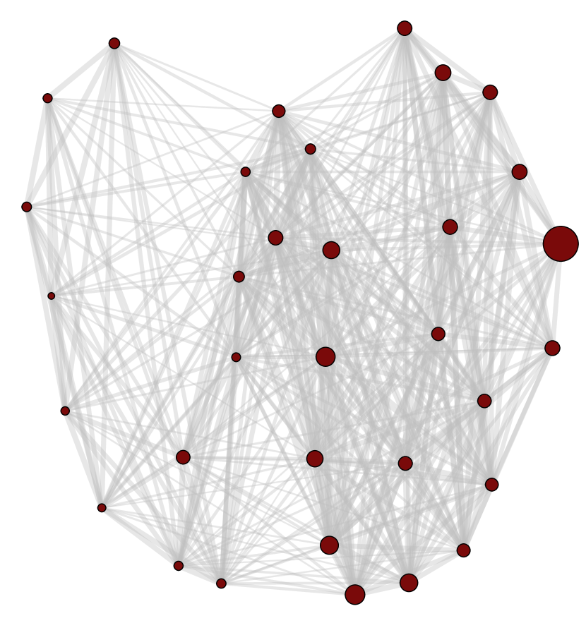
(a) Event Study With Staggered Entry

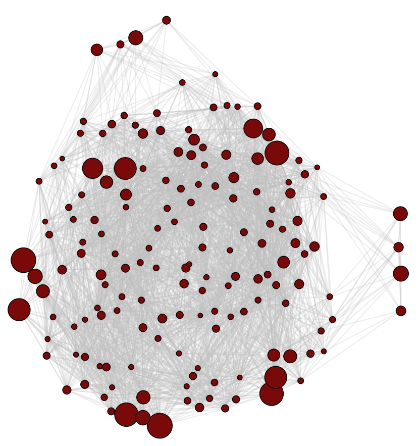
(b) Bipartite Match Outcomes

Figure E.1: These figures illustrate the observed outcome overlap graphs $\mathcal{G}_{1}$ corresponding to the empirical examples introduced in Section 1. Each red node corresponds to a cohort of units, the size of a node indicates the number of units in the corresponding cohort, an edge between two cohorts’ nodes exists if at least one of the same outcomes is observed for units in both cohorts, and the thickness of an edge corresponds to the number of overlapping observed outcomes between the cohorts whose corresponding nodes are connected by that edge. Figure 1(a) is generated using data from the longitudinal congestion pricing experiment studied in Ater . (), while Figure 1(b) is constructed from the VWH matched employer-employee dataset as discussed in Section 5.1.

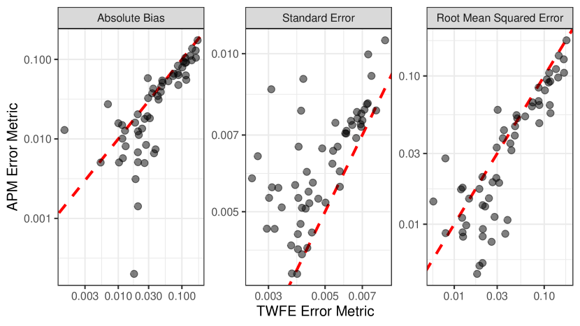
(a) Absolute Error Metrics

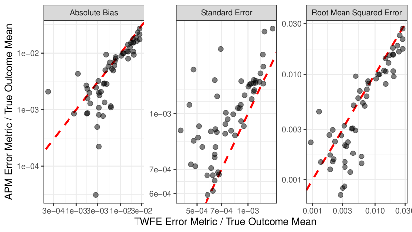
(b) Absolute Error Metrics Divded by True Outcome Means

Figure E.2: Each panel of Figure 2(a) shows a scatter plot of the values of an error metric for our estimator and the TWFE estimator, where each dot corresponds to one cohort outcome mean target parameter. Similarly, each panel of Figure 2(b) shows a scatter plot of the values of an error metric for our estimator and the TWFE estimator both normalized by the true value of the target parameters to which they correspond. If a dot in any panel of either subfigure lies below the 45-degree red dashed line, our estimator performs better on that error metric, and if not, then the TWFE estimator performs better on that error metric.

Appendix F Proofs of Supplementary Results

F.1 Preliminaries for and Proof of Theorem D.2

Preliminaries.

Let $\tilde{P}$ denote some distribution over $(C_{i},Y_{i}^{*})$, and let $\tilde{P}_{\text{obs}}$ denote the distribution over $(C_{i},Y_{i})$ implied by $\tilde{P}$. In addition, let $\Gamma(\tilde{P})$ denote the parameter $\Gamma$ implied by the distribution $\tilde{P}$. Assumption 4.1 implies that, for each cohort $c=1,\dotsc,C$, there exists a known function $\Pi(\tilde{\Gamma}_{c}(\tilde{P}_{\text{obs}}))$ mapping distributions over observables $\tilde{P}_{\text{obs}}$ to $\Pi(E_{c}\Gamma(\tilde{P}))$. We now strengthen Assumption 4.3 in the following manner:

Assumption F.1.

For each cohort $c=1,\dotsc,C$, the map $\Pi(\tilde{\Gamma}_{c}(\cdot))$ is Hadamard differentiable and satisfies $\Pi(\tilde{\Gamma}_{c}(\hat{P}_{N}))=\Pi(\hat{\Gamma}_{c})$.

We note that Assumption F.1 implies Assumption 4.3 by the Delta method (see e.g. Theorem 3.9.4 in van der Vaart  Wellner (1996)), the fact that $\hat{P}_{N}$ converges to $P$, and the fact that $\phi_{c}$ is the Riesz representer of the linear Hadamard derivative of $\Pi(\tilde{\Gamma}_{c}(\cdot))$.

Next, we let $\eta(\tilde{P})$ denote the value of the nuisance parameter implied by the distribution $\tilde{P}$, we let $\tilde{\eta}(\tilde{P}_{\text{obs}})$ be the representation of the consistent estimator $\hat{\eta}$ as a map from observable data distributions to estimate values. We can then also strengthen Assumption D.1 in a similar manner:

Assumption F.2.

The map $\tilde{\eta}(\cdot)$ is Hadamard differentiable and satisfies $\tilde{\eta}(\hat{P}_{N})=\hat{\eta}$.

Finally, we let $\tilde{\theta}(\tilde{P}_{\text{obs}})$ denote the mapping from observed data distributions $\tilde{P}_{\text{obs}}$ to target parameter values such that $\tilde{\theta}(\hat{P}_{N})=\hat{\theta}$. Given these definitions and assumptions, we are now equipped to prove Theorem D.2.

Proof.

First, we note that Assumption F.1, (A.24) from the proof of Theorem 4.4, (A.41) from the proof of Theorem 4.5, and Assumptions F.2 and D.2 allow us to apply the chain rule (see e.g. Lemma 3.9.3 in van der Vaart  Wellner (1996)) to say that the map $\tilde{\theta}(\cdot)$ is itself Hadamard differentiable.

Next, we note that the random weight vector $W$ satisfies Equation (3.6.8) in van der Vaart  Wellner (1996) by Example 3.6.9 in the same book. Thus, Theorem 3.6.13 in van der Vaart  Wellner (1996) implies that the Bayesian bootstrap yields a consistent estimate $\hat{P}_{N}^{*}$ of the true data-generating distribution $P_{\text{obs}}$, while the bootstrap delta method given in van der Vaart  Wellner (1996)’s Theorem 3.9.11 implies that the asymptotic distribution of $\hat{\theta}^{*}=\tilde{\theta}(\hat{P}_{N}^{*})$ converges to that of $\hat{\theta}$ in probability. Since quantile functions are also Hadamard differentiable (see Example 3.9.21 in van der Vaart  Wellner (1996)), we have that

$$\sqrt{N}\hat{\sigma}_{j}=\sqrt{\Sigma_{\theta,jj}}+o_{p}\left(1\right).$$ (F.1)

Given the bootstrap and standard error estimator consistency results above, we can appeal to Proposition 3 and Lemma 1 in the supplemental appendix of Montiel Olea  Plagborg-Møller (2019) to show that our confidence intervals have simultaneous coverage, as required.

F.2 Proof of Proposition D.3

First, we show that when $r=1$ and every entry of $\Gamma$ is non-zero, (4.1) reduces to the requirement that $\mathcal{T}_{c_{1}}\cap\mathcal{T}_{c_{2}}\neq\emptyset$, i.e. that cohorts $c_{1}$ and $c_{2}$ share at least one observed outcome. To see why, note that $E_{c_{1}}E_{c_{2}}\neq\operatorname{\mathbf{0}}$ whenever cohorts $c_{1}$ and $c_{2}$ share an observed outcome. Further, when $r=1$, the factor matrix $\Gamma$ is a column vector, in which case since, by assumption, every entry of $\Gamma$ is non-zero, $E_{c_{1}}E_{c_{2}}\Gamma\neq\operatorname{\mathbf{0}}$ if and only if cohorts $c_{1}$ and $c_{2}$ share an observed outcome. Thus, the rank of the column vector $E_{c_{1}}E_{c_{2}}\Gamma$ is exactly one if and only if cohorts $c_{1}$ and $c_{2}$ share an observed outcome. Thus, $\mathcal{G}_{1}$ has an edge between two cohorts if and only if they share at least one observed outcome.

Next, we will show that Assumption D.4 implies that $\mathcal{G}_{1}$ is connected. Under Assumption D.4, the connectedness of the bipartite $\tilde{\mathcal{G}}$ implies there must exist a sequence of edges with some length $\ell$ denoted

$$((i_{1},t_{1}),(i_{2},t_{1}),\dotsc,(i_{\ell-1},t_{\ell/2}),(i_{\ell},t_{\ell/2}))$$ (F.2)

between any two unit $i_{1}$ and $i_{\ell}$ in $\tilde{\mathcal{G}}$. Consider any pair of edges $(i_{j},t),(i_{j+1},t)$ in the path (F.2) that connect to the same outcome $t$. If $C_{i_{j}}\neq C_{i_{j+1}}$, i.e. that units $i_{j}$ and $i_{j+1}$ belong to different cohorts. Since the edges $(i_{j},t)$ and $(i_{j+1},t)$ both belong to $\tilde{\mathcal{G}}$, by definition, outcome $t$ is observed for $i_{j}$ and $i_{j+1}$, in which case cohorts $C_{i_{j}}$ and $C_{i_{j+1}}$ must share an edge in $\mathcal{G}_{1}$. If on the other hand $C_{i_{j}}=C_{i_{j+1}}$, then the same logic would imply there is a self-edge connected to $C_{i_{j}}$ if not for the fact that (4.1) only holds for pairs of distinct cohorts.

Based on the argument above, we can iteratively construct a length $\ell$ path in $\mathcal{G}_{1}$ corresponding to the path (F.2) in $\tilde{\mathcal{G}}$ that connects cohort $C_{i_{1}}$ to cohort $C_{i_{\ell}}$. Since connectedness of $\tilde{\mathcal{G}}$ implies that a path between any two units $i_{1}$ and $i_{2}$ exists in $\tilde{\mathcal{G}}$ and every cohort $c$ must have at least one unit belonging to it, any two cohorts in $\mathcal{G}_{1}$ must have a path between them. Thus, $\mathcal{G}_{1}$, must also be connected, so Assumption 4.2 must also hold.

Finally, we will show that if Assumption 4.4 also holds, then Assumption 4.2 implies Assumption D.4 holds with probability approaching one as $N\rightarrow\infty$. First, we note that since Assumption 4.4 requires a unit to belong to each cohort with positive probability and there are a finite number of cohorts, it must be that $\tilde{\mathcal{G}}$ contains a unit belonging to every cohort with probability approaching one as $N\rightarrow\infty$. As such, for the remainder of the proof, we shall condition on this event.

Next, under Assumption 4.2, $\mathcal{G}_{1}$ is connected, so there exists a sequence of edges with some length $\ell$ denoted

$$((c_{1},c_{2}),\dotsc,(c_{\ell-1},c_{\ell}))$$ (F.3)

that connects any two cohorts $c_{1}\neq c_{\ell}$. For a given edge $(c_{j},c_{j+1})$, consider any two units $i_{j}$ in cohort $c_{j}$ and $i_{j+1}$ in cohort $c_{j+1}$. Since the edge $(c_{j},c_{j+1})$ exists in $\mathcal{G}_{1}$, there must be at least one outcome $t_{j}$ that is observed for the units in both cohort $c_{j}$ and cohort $c_{j+1}$. As such, there must exist edges $(i_{j},t_{j})$ and $(i_{j+1},t_{j})$ in $\tilde{\mathcal{G}}$. Based on the argument above, we can iteratively construct a length $\ell$ path in $\tilde{\mathcal{G}}$ between any unit $i_{1}$ in cohort $c_{1}$ and any unit $i_{\ell}$ in cohort $c_{\ell}$.

To show that any two units $i_{1}$ and $i_{2}$ in the same cohort $c$ are connected in $\tilde{\mathcal{G}}$, we note that if the units are in the same cohort, the same set of outcomes is observed for both of them, meaning there exists at least one outcome $t$ such that the edges $(i_{1},t)$ and $(i_{2},t)$ exist. As such, there exists a length two path in $\tilde{\mathcal{G}}$ connecting any two units in the same cohort. In addition, since without loss of generality, every outcome is observed for at least one unit, for any outcome $t$, there exists at least one edge $(i,t)$ connecting it to some unit $i$. Putting everything together, we know that there exists a path in $\tilde{\mathcal{G}}$ connecting any two units, regardless of whether they belong to the same or different cohorts, and every outcome is connected to at least one unit. Thus, $\tilde{\mathcal{G}}$ must be connected, as required.

F.3 Proof of Proposition D.4

First, we will show that Assumption D.5 implies Assumption 4.2. Since $\check{\mathcal{G}}$ is connected, there exists a path in $\check{\mathcal{G}}$ of some length $\ell$ denoted

$$((t_{1},t_{2}),\dotsc,(t_{\ell},t_{\ell+1}))$$ (F.4)

between any two outcomes $t_{1}$ and $t_{\ell}$. If $\ell=1$, that directly implies the existence of a cohort of units for whom outcomes $t_{1}$ and $t_{\ell}=t_{2}$ are both observed.

If $\ell\geq 2$ on the other hand, consider any two adjacent edges $(t_{j},t_{j+1})$ and $(t_{j+1},t_{j+2})$ in the path (F.4). Since the edge $(t_{j},t_{j+1})$ exists in $\check{\mathcal{G}}$, there must be some cohort of units $c_{j}$ for whom both outcomes $t_{j}$ and $t_{j+1}$ are observed. By similar logic, there must be some cohort of units $c_{j+1}$ for whom both outcomes $t_{j+1}$ and $t_{j+2}$ are observed. Since outcome $t_{j+1}$ is observed for the units in cohorts $c_{j}$ and $c_{j+1}$, they must then share an edge in $\mathcal{G}_{1}$ (see the proof of Proposition D.3 in Appendix F.2 to see why we need to assume all entries of $\Gamma$ are non-zero). Applying this logic iteratively along the path in (F.4), we can construct a path in $\mathcal{G}_{1}$ from any cohort for whom outcome $t_{1}$ is observed to any cohort for whom outcome $t_{\ell}$ is observed. Since without loss, at least one outcome is observed for the units in every cohort, we can therefore construct a path in $\mathcal{G}_{1}$ between any pair of cohorts, meaning $\mathcal{G}_{1}$ is connected.

Next, we show that Assumption 4.2 implies Assumption D.5. Since $\mathcal{G}_{1}$ is connected, there exists a path in $\mathcal{G}_{1}$ of some length $\ell$ denoted

$$((c_{1},c_{2}),\dotsc,(c_{\ell-1},c_{\ell}))$$ (F.5)

between any two cohorts $c_{1}$ and $c_{\ell}$. For a given edge $(c_{j},c_{j+1})$ in $\mathcal{G}_{1}$, by definition, there must be some outcome $t_{j}$ that is observed for both of the positive measures of units in cohorts $c_{j}$ and $c_{j+1}$ by Assumption 4.4. Thus, for any outcome observed for the units in $c_{j}$, there must be an edge in $\check{\mathcal{G}}$ between it and $t_{j}$, and similarly, for any outcome observed for the units in $c_{j+1}$, there must be an edge in $\check{\mathcal{G}}$ between it and $t_{j}$. Thus, a path of length two exists in $\check{\mathcal{G}}$ between any outcome observed for the units in $c_{j}$ and any outcome observed for the units in $c_{j+1}$. Applying this same logic iteratively along the path (F.5), a path can be constructed in $\check{\mathcal{G}}$ connecting any outcome observed for the units in cohort $c_{1}$ to any outcome observed for the units in cohort $c_{\ell}$. Since without loss of generality, every outcome is observed for the units in at least one cohort, a path in $\check{\mathcal{G}}$ can be constructed between any two outcomes. Thus, $\check{\mathcal{G}}$ is connected, as required.

F.4 Proof of Lemma D.5

Let $U_{\Gamma}S_{\Gamma}V_{\Gamma}^{\prime}$ be a compact singular value decomposition of $E_{c}\Gamma$, and recall that, by Lemma 4.1, $E_{c}\Gamma$ is rank $r$. Next, note that

$$V_{c} =E_{c}\operatorname{\mathbb{E}}[Y_{i}^{*}(Y_{i}^{*})^{\prime}~{}|~{}C_{i}=c]E_{c}$$ (F.6)

$$=E_{c}\big{(}\Gamma\operatorname{\mathbb{E}}[\lambda_{i}\lambda_{i}^{\prime}~{}|~{}C_{i}=c]\Gamma^{\prime}+\operatorname{\mathbb{E}}[\operatorname{\varepsilon}_{i}\operatorname{\varepsilon}_{i}^{\prime}~{}|~{}C_{i}=c]$$ (F.7)

$$\phantom{=E_{c}\big{(}}+\Gamma\operatorname{\mathbb{E}}[\lambda_{i}\operatorname{\varepsilon}_{i}^{\prime}~{}|~{}C_{i}=c]+\operatorname{\mathbb{E}}[\operatorname{\varepsilon}_{i}\lambda_{i}^{\prime}~{}|~{}C_{i}=c]\Gamma^{\prime}\big{)}E_{c}$$ (by (2.2)) (F.8)

$$=E_{c}\left(\Gamma\operatorname{\mathbb{E}}[\lambda_{i}\lambda_{i}^{\prime}~{}|~{}C_{i}=c]\Gamma^{\prime}+\operatorname{\mathbb{E}}[\operatorname{\varepsilon}_{i}\operatorname{\varepsilon}_{i}^{\prime}~{}|~{}C_{i}=c]\right)E_{c} \operatorname{\mathbb{E}}[\operatorname{\varepsilon}_{i}~{}|~{}\lambda_{i},C_{i}]=\operatorname{\mathbf{0}}$$ ( by (2.2)) (F.9)

$$=E_{c}\left(\Gamma\operatorname{\mathbb{E}}[\lambda_{i}\lambda_{i}^{\prime}~{}|~{}C_{i}=c]\Gamma^{\prime}+\underbrace{\operatorname{\mathbb{E}}[\sigma_{i}^{2}~{}|~{}C_{i}=c]}_{\sigma_{c}^{2}}I\right)E_{c}$$ (by Assumption D.7) (F.10)

$$=U_{\Gamma}\underbrace{S_{\Gamma}V_{\Gamma}^{\prime}\operatorname{\mathbb{E}}[\lambda_{i}\lambda_{i}^{\prime}~{}|~{}C_{i}=c]V_{\Gamma}S_{\Gamma}}_{M}U_{\Gamma}^{\prime}+\sigma_{c}^{2}E_{c}. E_{c}\Gamma=U_{\Gamma}S_{\Gamma}V_{\Gamma}$$ () (F.11)

Now, let $U_{M}S_{M}^{2}U_{M}^{\prime}$ denote an eigendecomposition of the $r\times r$ matrix $M$ in the display above, and note that since the $r\times r$ matrix $\operatorname{\mathbb{E}}[\lambda_{i}\lambda_{i}^{\prime}~{}|~{}C_{i}=c]$ is rank $r$ by Assumption D.6 and so is $E_{c}\Gamma$ by Lemma 4.1, $S_{M}^{2}$ has $r$ non-zero eigenvalues. Then we have that

$$V_{c}=U_{\Gamma}U_{M}S_{M}^{2}U_{M}^{\prime}U_{\Gamma}^{\prime}+\sigma_{c}^{2}E_{c}.$$ (F.12)

Since $U_{M}$ is an orthonormal matrix and the columns of $U_{\Gamma}$ are orthonormal to one another, $U_{\Gamma}U_{M}$ must also have $r$ orthonormal columns. Further, we will show that $E_{c}U_{\Gamma}=U_{\Gamma}$, in which case $E_{c}U_{\Gamma}U_{M}=U_{\Gamma}U_{M}$. To see why, note that

$$E_{c}\Gamma\Gamma^{\prime}E_{c}\cdot E_{c}U_{\Gamma} =E_{c}\cdot E_{c}\Gamma\Gamma^{\prime}E_{c}\cdot U_{\Gamma} E_{c}$$ ( is idempotent) (F.13)

$$=E_{c}U_{\Gamma}S_{\Gamma}V_{\Gamma}^{\prime}V_{\Gamma}S_{\Gamma}U_{\Gamma}^{\prime}U_{\Gamma} E_{c}\Gamma=U_{\Gamma}S_{\Gamma}V_{\Gamma}^{\prime}$$ () (F.14)

$$=E_{c}U_{\Gamma}S_{\Gamma}^{2}. V_{\Gamma}^{\prime}V_{\Gamma}=U_{\Gamma}^{\prime}U_{\Gamma}=I$$ () (F.15)

Thus, $E_{c}U_{\Gamma}$ are eigenvectors corresponding to the $r$ non-zero eigenvalues of $E_{c}\Gamma\Gamma^{\prime}E_{c}$, so they must also be left singular vectors of $E_{c}\Gamma$.

Next, let $U_{Y1}\coloneqq E_{c}U_{\Gamma}U_{M}$, let $U_{Y2}$ be a $T\times(\lvert\mathcal{T}_{c}\rvert-r)$ matrix with orthonormal columns such that $U_{Y1}^{\prime}U_{Y2}=\operatorname{\mathbf{0}}$ and $E_{c}U_{Y2}=U_{Y2}$, i.e. the columns of $U_{Y2}$ are orthogonal to the columns of $U_{Y1}$, and $U_{Y2}$ only has non-zero entries in the indices $\mathcal{T}_{c}$, and let $U_{Y3}$ be a $T\times(T-\lvert\mathcal{T}_{c}\rvert)$ matrix such that

$$U_{Y}\coloneqq\begin{bmatrix}U_{Y1}&U_{Y2}&U_{Y3}\end{bmatrix}\eqqcolon\begin{bmatrix}U_{Yc}&U_{Y3}\end{bmatrix}$$ (F.16)

is orthonormal. We note that the existence of the aforementioned matrices is guaranteed constructively by applications of the Gram-Schmidt process. By construction, since $U_{Y}U_{Y}^{\prime}=I$ and $U_{Yc}$ has orthonormal columns with non-zero entries only in the indices $\mathcal{T}_{c}$, it must be that $U_{Yc}U_{Yc}^{\prime}=E_{c}$ and $U_{Y3}U_{Y3}^{\prime}=I-E_{c}$. Then, expanding the right side of (F.12) using these matrices, we have that

$$V_{c} =\begin{bmatrix}U_{Y1}&\begin{bmatrix}U_{Y2}&U_{Y3}\end{bmatrix}\end{bmatrix}\begin{bmatrix}S_{M}^{2}&\operatorname{\mathbf{0}}_{r\times(T-r)}\\ \operatorname{\mathbf{0}}_{(T-r)\times r}&\operatorname{\mathbf{0}}_{(T-r)\times(T-r)}\end{bmatrix}\begin{bmatrix}U_{Y1}^{\prime}\\ \begin{bmatrix}U_{Y2}^{\prime}\\ U_{Y3}^{\prime}\end{bmatrix}\end{bmatrix}$$ (F.17)

$$\phantom{=}+\begin{bmatrix}U_{Yc}&U_{Y3}\end{bmatrix}\begin{bmatrix}\sigma_{c}^{2}I_{\lvert\mathcal{T}_{c}\rvert}&\operatorname{\mathbf{0}}_{\lvert\mathcal{T}_{c}\rvert\times(T-\lvert\mathcal{T}_{c}\rvert)}\\ \operatorname{\mathbf{0}}_{(T-\lvert\mathcal{T}_{c}\rvert)\times\lvert\mathcal{T}_{c}\rvert}&\operatorname{\mathbf{0}}_{(T-\lvert\mathcal{T}_{c}\rvert)\times(T-\lvert\mathcal{T}_{c}\rvert)}\end{bmatrix}\begin{bmatrix}U_{Yc}^{\prime}\\ U_{Y3}^{\prime}\end{bmatrix}$$ (F.18)

$$=\underbrace{\begin{bmatrix}U_{Y1}&U_{Y2}&U_{Y3}\end{bmatrix}}_{U_{Y}}\begin{bmatrix}S_{M}^{2}+\sigma_{c}^{2}I_{r}&\operatorname{\mathbf{0}}&\operatorname{\mathbf{0}}\\ \operatorname{\mathbf{0}}&\sigma_{c}^{2}I_{\lvert\mathcal{T}_{c}\rvert-r}&\operatorname{\mathbf{0}}\\ \operatorname{\mathbf{0}}&\operatorname{\mathbf{0}}&\operatorname{\mathbf{0}}\end{bmatrix}\underbrace{\begin{bmatrix}U_{Y1}^{\prime}\\ U_{Y2}^{\prime}\\ U_{Y3}^{\prime}\end{bmatrix}}_{U_{Y}^{\prime}}.$$ (F.19)

Since $U_{Y}$ is an orthonormal matrix, the center matrix in the last line of the display above is diagonal, and the diagonal entries of $S_{M}^{2}+\sigma_{c}^{2}I_{r}$ are strictly larger than those of $\sigma_{c}^{2}I_{\lvert\mathcal{T}_{c}\rvert-r}$ from the fact that $S_{M}$ is positive definite, the expression in the display above must be an eigendecomposition of $V_{c}$.

Because the eigenvalues of products of nonsingular square matrices are invariant to cyclic permutations of the product terms, the eigenvalues of the matrices $S_{\Gamma}V_{\Gamma}^{\prime}\operatorname{\mathbb{E}}[\lambda_{i}\lambda_{i}^{\prime}~{}|~{}C_{i}=c]V_{\Gamma}S_{\Gamma}$ and $V_{\Gamma}S_{\Gamma}^{2}V_{\Gamma}^{\prime}\operatorname{\mathbb{E}}[\lambda_{i}\lambda_{i}^{\prime}~{}|~{}C_{i}=c]$ are the same. Since $S_{M}^{2}$ is the diagonal matrix whose non-zero entries are the ordered eigenvalues of $S_{\Gamma}V_{\Gamma}^{\prime}\operatorname{\mathbb{E}}[\lambda_{i}\lambda_{i}^{\prime}~{}|~{}C_{i}=c]V_{\Gamma}S_{\Gamma}$, and $V_{\Gamma}S_{\Gamma}^{2}V_{\Gamma}^{\prime}=\Gamma^{\prime}E_{c}\cdot E_{c}\Gamma=\Gamma^{\prime}E_{c}\Gamma$, we equivalently have that $S_{M}^{2}$ is the diagonal matrix whose non-zero entries are the ordered eigenvalues of $\Gamma^{\prime}E_{c}\Gamma\operatorname{\mathbb{E}}[\lambda_{i}\lambda_{i}^{\prime}~{}|~{}C_{i}=c]$. The results stated in the statement of the lemma then follow from the fact that $\Pi(U_{Y1})=\Pi(E_{c}U_{\Gamma}U_{M})=\Pi(U_{\Gamma})=\Pi(E_{c}\Gamma)$ and inspection of the eigendecomposition.

F.5 Proof of Proposition D.6

First, we note that under Assumptions 4.4 and D.6, a classical multivariate Central Limit Theorem dictates that $\mathrm{vec}(\hat{V}_{c}-V_{c})=O_{p}\left(N^{-1/2}\right)$, so

$$\lVert\hat{V}_{c}-V_{c}\rVert_{\text{op}} \leq\lVert\hat{V}_{c}-V_{c}\rVert_{F}$$ (F.20)

$$=\lVert\mathrm{vec}(\hat{V}_{c}-V_{c})\rVert_{2}$$ (F.21)

$$=O_{p}\left(N^{-1/2}\right).$$ (F.22)

Next, we apply Theorem B.1 with $M=V_{c}$, $\hat{M}=\hat{V}_{c}$, $s=T-r$, and $r=r$. Lemma D.5 implies that, using the notation from Appendix B,

$$\lambda_{T-r}(V_{c})=\sigma_{c}^{2}<s_{1c}^{2}+\sigma_{c}^{2}=\lambda_{T-r+1}(V_{c})\leq\dotsc s_{rc}^{2}+\sigma_{c}^{2}=\lambda_{T}(V_{c})<\lambda_{T+1}(V_{c})=\infty.$$ (F.23)

As such, we have that $\Delta(V_{c})=4^{-1}s_{1c}^{2}>0$, satisfying (B.4). Lemma D.5 also implies that, for $j\in\{T-r+1,\dotsc,T\}$ and $k\in\{1,\dotsc,T-r\}$,

$$\lambda_{j}-\lambda_{k}=s_{(j-(T-r))c}^{2}+\sigma_{c}^{2}\mathbbm{1}\{k\leq T-\lvert\mathcal{T}_{c}\rvert\}.$$ (F.24)

Further, Lemma D.5 implies that

$$\Pi(E_{c}\Gamma)=\Pi(U_{(T-r+1):T}(V_{c}))$$ (F.25)

and we define $\hat{\Gamma}_{c,\text{PC}}$ such that

$$\Pi(\hat{\Gamma}_{c,\text{PC}})=\Pi(U_{(T-r+1):T}(\hat{V}_{c})).$$ (F.26)

Then so long as

$$\lVert\hat{V}_{c}-V_{c}\rVert_{\text{op}}\leq 4^{-1}s_{1c}^{2},$$ (F.27)

Theorem B.1 implies that

$$\Bigg{\lVert}\Pi(\hat{\Gamma}_{c,\text{PC}})-\Pi(E_{c}\Gamma)$$ (F.28)

$$\phantom{\Bigg{\lVert}}-\sum_{j=T-r+1}^{T}\sum_{k=1}^{T-r}\frac{-1}{s_{(j-(T-r))c}^{2}+\sigma_{c}^{2}\mathbbm{1}\{k\leq T-\lvert\mathcal{T}_{c}\rvert\}}$$

$$\phantom{\Bigg{\lVert}-\sum_{j=T-r+1}^{T}\sum_{k=1}^{T-r}}\cdot\left[\Pi(\tilde{\gamma}_{cj})(\hat{V}_{c}-V_{c})\Pi(\tilde{\gamma}_{ck})+\Pi(\tilde{\gamma}_{ck})(\hat{V}_{c}-V_{c})\Pi(\tilde{\gamma}_{cj})\right]\Bigg{\rVert}_{\text{op}}$$

$$\leq\frac{64}{\pi s_{1c}^{4}}\lVert\hat{V}_{c}-V_{c}\rVert_{\text{op}}^{2}.$$

The fact that $\lVert\hat{V}_{c}-V_{c}\rVert_{\text{op}}=O_{p}\left(N^{-1/2}\right)$ implies (F.27) holds with probability approaching one as $N\rightarrow\infty$, so by the display above,

$$\Pi(\hat{\Gamma}_{c,\text{PC}})-\Pi(E_{c}\Gamma)$$ (F.29)

$$=\sum_{j=T-r+1}^{T}\sum_{k=1}^{T-r}\frac{-1}{s_{(j-(T-r))c}^{2}+\sigma_{c}^{2}\mathbbm{1}\{k\leq T-\lvert\mathcal{T}_{c}\rvert\}}\bigg{\{}\Pi(\tilde{\gamma}_{cj})(\hat{V}_{c}-V_{c})\Pi(\tilde{\gamma}_{ck})$$

$$\phantom{=\sum_{j=T-r+1}^{T}\sum_{k=1}^{T-r}\frac{1}{s_{(j-(T-r))c}^{2}+\sigma_{c}^{2}\mathbbm{1}\{k\leq T-\lvert\mathcal{T}_{c}\rvert\}}\bigg{\{}}+\Pi(\tilde{\gamma}_{ck})(\hat{V}_{c}-V_{c})\Pi(\tilde{\gamma}_{cj})\bigg{\}}$$

$$\phantom{=}+o_{p}\left(N^{-1/2}\right).$$

Applying (A.32) to $\sqrt{N}$ times the vectorization of both sides of (F.29), since $\Pi(\cdot)$ must be symmetric,

$$\sqrt{N}\mathrm{vec}\left(\Pi(\hat{\Gamma}_{c,\text{PC}})-\Pi(E_{c}\Gamma)\right)$$ (F.30)

$$=\sum_{j=T-r+1}^{T}\sum_{k=1}^{T-r}\frac{-1}{s_{(j-(T-r))c}^{2}+\sigma_{c}^{2}\mathbbm{1}\{k\leq T-\lvert\mathcal{T}_{c}\rvert\}}\left[\Pi(\tilde{\gamma}_{cj})\otimes\Pi(\tilde{\gamma}_{ck})+\Pi(\tilde{\gamma}_{ck})\otimes\Pi(\tilde{\gamma}_{cj})\right]$$

$$\phantom{=}\cdot\sqrt{N}\mathrm{vec}\left(\hat{V}_{c}-V_{c}\right)+o_{p}\left(N^{-1/2}\right).$$

(D.17), $\operatorname{\mathbb{E}}[\phi_{c}(C_{i},Y_{i})]=\operatorname{\mathbf{0}}_{T^{2}}$ and the boundedness of the expected squared norm of $\phi_{c}$ then follow from the expansion of $\hat{V}_{c}-V_{c}$ implied by Lemma A.2, the fact that $H_{c}$ certainly has bounded operator norm (since $s_{(j-(T-r))c}^{2}+\sigma_{c}^{2}\mathbbm{1}\{k\leq T-\lvert\mathcal{T}_{c}\rvert\}>0$), and Assumption 4.4.

References

• Abadie \BOthers. (\APACyear2010) \APACinsertmetastarabadie2010synthetic{APACrefauthors}Abadie, A., Diamond, A.\BCBL \BBA Hainmueller, J.  \APACrefYearMonthDay2010. \BBOQ\APACrefatitleSynthetic control methods for comparative case studies: Estimating the effect of California’s tobacco control program Synthetic control methods for comparative case studies: Estimating the effect of california’s tobacco control program.\BBCQ \APACjournalVolNumPagesJournal of the American Statistical Association105490493–505.
• Abowd \BOthers. (\APACyear2002) \APACinsertmetastarabowd2002computing{APACrefauthors}Abowd, J\BPBIM., Creecy, R\BPBIH.\BCBL \BBA Kramarz, F.  \APACrefYearMonthDay2002. \APACrefbtitleComputing person and firm effects using linked longitudinal employer-employee data Computing person and firm effects using linked longitudinal employer-employee data \APACbVolEdTR\BTR. \APACaddressInstitutionCenter for Economic Studies, US Census Bureau.
• Abowd \BOthers. (\APACyear1999) \APACinsertmetastarabowd1999high{APACrefauthors}Abowd, J\BPBIM., Kramarz, F.\BCBL \BBA Margolis, D\BPBIN.  \APACrefYearMonthDay1999. \BBOQ\APACrefatitleHigh wage workers and high wage firms High wage workers and high wage firms.\BBCQ \APACjournalVolNumPagesEconometrica672251–333.
• Agarwal, Dahleh\BCBL \BOthers. (\APACyear2023) \APACinsertmetastaragarwal2021causal{APACrefauthors}Agarwal, A., Dahleh, M., Shah, D.\BCBL \BBA Shen, D.  \APACrefYearMonthDay2023. \BBOQ\APACrefatitleCausal matrix completion Causal matrix completion.\BBCQ \BIn \APACrefbtitleThe Thirty Sixth Annual Conference on Learning Theory The thirty sixth annual conference on learning theory (\BPGS 3821–3826).
• Agarwal, Shah\BCBL \BBA Shen (\APACyear2023) \APACinsertmetastaragarwal2020synthetic{APACrefauthors}Agarwal, A., Shah, D.\BCBL \BBA Shen, D.  \APACrefYearMonthDay2023. \BBOQ\APACrefatitleSynthetic Interventions Synthetic interventions.\BBCQ \APACjournalVolNumPagesarXiv preprint arXiv:2006.07691.
• Ahn \BBA Horenstein (\APACyear2013) \APACinsertmetastarahn2013eigenvalue{APACrefauthors}Ahn, S\BPBIC.\BCBT \BBA Horenstein, A\BPBIR.  \APACrefYearMonthDay2013. \BBOQ\APACrefatitleEigenvalue ratio test for the number of factors Eigenvalue ratio test for the number of factors.\BBCQ \APACjournalVolNumPagesEconometrica8131203–1227.
• Ahn \BOthers. (\APACyear2013) \APACinsertmetastarahn2013panel{APACrefauthors}Ahn, S\BPBIC., Lee, Y\BPBIH.\BCBL \BBA Schmidt, P.  \APACrefYearMonthDay2013. \BBOQ\APACrefatitlePanel data models with multiple time-varying individual effects Panel data models with multiple time-varying individual effects.\BBCQ \APACjournalVolNumPagesJournal of Econometrics17411–14.
• Anderson (\APACyear1963) \APACinsertmetastaranderson1963asymptotic{APACrefauthors}Anderson, T\BPBIW.  \APACrefYearMonthDay1963. \BBOQ\APACrefatitleAsymptotic theory for principal component analysis Asymptotic theory for principal component analysis.\BBCQ \APACjournalVolNumPagesThe Annals of Mathematical Statistics341122–148.
• Anderson (\APACyear2009) \APACinsertmetastaranderson2009introduction{APACrefauthors}Anderson, T\BPBIW.  \APACrefYear2009. \APACrefbtitleAn Introduction to Multivariate Statistical Analysis, 3rd Edition An introduction to multivariate statistical analysis, 3rd edition. \APACaddressPublisherWiley-Interscience.
• Anderson \BBA Rubin (\APACyear1956) \APACinsertmetastaranderson1956statistical{APACrefauthors}Anderson, T\BPBIW.\BCBT \BBA Rubin, H.  \APACrefYearMonthDay1956. \BBOQ\APACrefatitleStatistical Inference in Factor Analysis Statistical inference in factor analysis.\BBCQ \BIn \APACrefbtitleProceedings of the Third Berkeley Symposium on Mathematical Statistics and Probability: Held at the Statistical Laboratory, University of California, December, 1954, July and August, 1955 Proceedings of the third berkeley symposium on mathematical statistics and probability: Held at the statistical laboratory, university of california, december, 1954, july and august, 1955 (\BVOL 1, \BPG 111).
• Andrews \BOthers. (\APACyear2008) \APACinsertmetastarandrews2008high{APACrefauthors}Andrews, M\BPBIJ., Gill, L., Schank, T.\BCBL \BBA Upward, R.  \APACrefYearMonthDay2008. \BBOQ\APACrefatitleHigh wage workers and low wage firms: negative assortative matching or limited mobility bias? High wage workers and low wage firms: negative assortative matching or limited mobility bias?\BBCQ \APACjournalVolNumPagesJournal of the Royal Statistical Society: Series A (Statistics in Society)1713673–697.
• Angrist \BBA Pischke (\APACyear2009) \APACinsertmetastarangrist2009mostly{APACrefauthors}Angrist, J\BPBID.\BCBT \BBA Pischke, J\BHBIS.  \APACrefYear2009. \APACrefbtitleMostly harmless econometrics: An empiricist’s companion Mostly harmless econometrics: An empiricist’s companion. \APACaddressPublisherPrinceton university press.
• Arkhangelsky \BOthers. (\APACyear2021) \APACinsertmetastararkhangelsky2021synthetic{APACrefauthors}Arkhangelsky, D., Athey, S., Hirshberg, D\BPBIA., Imbens, G\BPBIW.\BCBL \BBA Wager, S.  \APACrefYearMonthDay2021. \BBOQ\APACrefatitleSynthetic difference-in-differences Synthetic difference-in-differences.\BBCQ \APACjournalVolNumPagesAmerican Economic Review111124088–4118.
• Arkhangelsky \BBA Hirshberg (\APACyear2023) \APACinsertmetastararkhangelsky2023largesample{APACrefauthors}Arkhangelsky, D.\BCBT \BBA Hirshberg, D.  \APACrefYearMonthDay2023. \BBOQ\APACrefatitleLarge-Sample Properties of the Synthetic Control Method under Selection on Unobservables Large-sample properties of the synthetic control method under selection on unobservables.\BBCQ \APACjournalVolNumPagesarXiv preprint arXiv:2311.13575.
• Ashenfelter \BBA Card (\APACyear1985) \APACinsertmetastarashenfelter1985using{APACrefauthors}Ashenfelter, O.\BCBT \BBA Card, D.  \APACrefYearMonthDay1985. \BBOQ\APACrefatitleUsing the longitudinal structure of earnings to estimate the effect of training programs Using the longitudinal structure of earnings to estimate the effect of training programs.\BBCQ \APACjournalVolNumPagesThe Review of Economics and Statistics674648–660.
• Ater \BOthers. (\APACyear\bibnodate) \APACinsertmetastarater2023can{APACrefauthors}Ater, I., Shany, A., Ross, B., Turkel, E.\BCBL \BBA Vasserman, S.  \APACrefYearMonthDay\bibnodate. \BBOQ\APACrefatitleCan usage-based pricing reduce traffic congestion? Can usage-based pricing reduce traffic congestion?\BBCQ \APACjournalVolNumPagesWork in progress.
• Athey \BOthers. (\APACyear2021) \APACinsertmetastarathey2021matrix{APACrefauthors}Athey, S., Bayati, M., Doudchenko, N., Imbens, G\BPBIW.\BCBL \BBA Khosravi, K.  \APACrefYearMonthDay2021. \BBOQ\APACrefatitleMatrix completion methods for causal panel data models Matrix completion methods for causal panel data models.\BBCQ \APACjournalVolNumPagesJournal of the American Statistical Association1165361716–1730.
• J. Bai (\APACyear2003) \APACinsertmetastarbai2003inferential{APACrefauthors}Bai, J.  \APACrefYearMonthDay2003. \BBOQ\APACrefatitleInferential theory for factor models of large dimensions Inferential theory for factor models of large dimensions.\BBCQ \APACjournalVolNumPagesEconometrica711135–171.
• J. Bai \BBA Ng (\APACyear2002) \APACinsertmetastarbai2002determining{APACrefauthors}Bai, J.\BCBT \BBA Ng, S.  \APACrefYearMonthDay2002. \BBOQ\APACrefatitleDetermining the number of factors in approximate factor models Determining the number of factors in approximate factor models.\BBCQ \APACjournalVolNumPagesEconometrica701191–221.
• J. Bai \BBA Ng (\APACyear2013) \APACinsertmetastarbai2013principal{APACrefauthors}Bai, J.\BCBT \BBA Ng, S.  \APACrefYearMonthDay2013. \BBOQ\APACrefatitlePrincipal components estimation and identification of static factors Principal components estimation and identification of static factors.\BBCQ \APACjournalVolNumPagesJournal of Econometrics176118–29.
• J. Bai \BBA Ng (\APACyear2021) \APACinsertmetastarbai2021matrix{APACrefauthors}Bai, J.\BCBT \BBA Ng, S.  \APACrefYearMonthDay2021. \BBOQ\APACrefatitleMatrix completion, counterfactuals, and factor analysis of missing data Matrix completion, counterfactuals, and factor analysis of missing data.\BBCQ \APACjournalVolNumPagesJournal of the American Statistical Association1165361746–1763.
• J. Bai \BBA Ng (\APACyear2023) \APACinsertmetastarbai2021approximate{APACrefauthors}Bai, J.\BCBT \BBA Ng, S.  \APACrefYearMonthDay2023. \BBOQ\APACrefatitleApproximate factor models with weaker loadings Approximate factor models with weaker loadings.\BBCQ \APACjournalVolNumPagesJournal of Econometrics.
• Z. Bai \BBA Silverstein (\APACyear2010) \APACinsertmetastarbai2010spectral{APACrefauthors}Bai, Z.\BCBT \BBA Silverstein, J\BPBIW.  \APACrefYear2010. \APACrefbtitleSpectral analysis of large dimensional random matrices Spectral analysis of large dimensional random matrices (\BVOL 20). \APACaddressPublisherSpringer.
• Belloni \BOthers. (\APACyear2017) \APACinsertmetastarbelloni2017program{APACrefauthors}Belloni, A., Chernozhukov, V., Fernandez-Val, I.\BCBL \BBA Hansen, C.  \APACrefYearMonthDay2017. \BBOQ\APACrefatitleProgram evaluation and causal inference with high-dimensional data Program evaluation and causal inference with high-dimensional data.\BBCQ \APACjournalVolNumPagesEconometrica851233–298.
• Ben-Michael \BOthers. (\APACyear2022) \APACinsertmetastarben2022synthetic{APACrefauthors}Ben-Michael, E., Feller, A.\BCBL \BBA Rothstein, J.  \APACrefYearMonthDay2022. \BBOQ\APACrefatitleSynthetic controls with staggered adoption Synthetic controls with staggered adoption.\BBCQ \APACjournalVolNumPagesJournal of the Royal Statistical Society Series B842351–381.
• Bertrand \BOthers. (\APACyear2004) \APACinsertmetastarbertrand2004much{APACrefauthors}Bertrand, M., Duflo, E.\BCBL \BBA Mullainathan, S.  \APACrefYearMonthDay2004. \BBOQ\APACrefatitleHow much should we trust differences-in-differences estimates? How much should we trust differences-in-differences estimates?\BBCQ \APACjournalVolNumPagesThe Quarterly Journal of Economics1191249–275.
• Bertsimas \BOthers. (\APACyear2017) \APACinsertmetastarbertsimas2017certifiably{APACrefauthors}Bertsimas, D., Copenhaver, M\BPBIS.\BCBL \BBA Mazumder, R.  \APACrefYearMonthDay2017. \BBOQ\APACrefatitleCertifiably optimal low rank factor analysis Certifiably optimal low rank factor analysis.\BBCQ \APACjournalVolNumPagesThe Journal of Machine Learning Research181907–959.
• Bing \BOthers. (\APACyear2022) \APACinsertmetastarbing2022inference{APACrefauthors}Bing, X., Bunea, F.\BCBL \BBA Wegkamp, M.  \APACrefYearMonthDay2022. \BBOQ\APACrefatitleInference in latent factor regression with clusterable features Inference in latent factor regression with clusterable features.\BBCQ \APACjournalVolNumPagesBernoulli282997–1020.
• Bonhomme (\APACyear2020) \APACinsertmetastarbonhomme2020econometric{APACrefauthors}Bonhomme, S.  \APACrefYearMonthDay2020. \BBOQ\APACrefatitleEconometric analysis of bipartite networks Econometric analysis of bipartite networks.\BBCQ \BIn \APACrefbtitleThe econometric analysis of network data The econometric analysis of network data (\BPGS 83–121). \APACaddressPublisherElsevier.
• Bonhomme \BOthers. (\APACyear2023) \APACinsertmetastarbonhomme2023much{APACrefauthors}Bonhomme, S., Holzheu, K., Lamadon, T., Manresa, E., Mogstad, M.\BCBL \BBA Setzler, B.  \APACrefYearMonthDay2023. \BBOQ\APACrefatitleHow much should we trust estimates of firm effects and worker sorting? How much should we trust estimates of firm effects and worker sorting?\BBCQ \APACjournalVolNumPagesJournal of Labor Economics412291–322.
• Bonhomme \BOthers. (\APACyear2019) \APACinsertmetastarbonhomme2019distributional{APACrefauthors}Bonhomme, S., Lamadon, T.\BCBL \BBA Manresa, E.  \APACrefYearMonthDay2019. \BBOQ\APACrefatitleA distributional framework for matched employer employee data A distributional framework for matched employer employee data.\BBCQ \APACjournalVolNumPagesEconometrica873699–739.
• Borusyak \BOthers. (\APACyear2023) \APACinsertmetastarborusyak2021revisiting{APACrefauthors}Borusyak, K., Jaravel, X.\BCBL \BBA Spiess, J.  \APACrefYearMonthDay2023. \BBOQ\APACrefatitleRevisiting event study designs: Robust and efficient estimation Revisiting event study designs: Robust and efficient estimation.\BBCQ \APACjournalVolNumPagesReview of Economic Studies.
• Brown \BBA Butts (\APACyear2022) \APACinsertmetastarbrown2022generalized{APACrefauthors}Brown, N.\BCBT \BBA Butts, K.  \APACrefYearMonthDay2022. \BBOQ\APACrefatitleGeneralized Imputation Estimators for Factor Models Generalized imputation estimators for factor models.\BBCQ
• Brown \BOthers. (\APACyear2023) \APACinsertmetastarbrown2023difference{APACrefauthors}Brown, N., Butts, K.\BCBL \BBA Westerlund, J.  \APACrefYearMonthDay2023. \BBOQ\APACrefatitleDifference-in-Differences via Common Correlated Effects Difference-in-differences via common correlated effects.\BBCQ \APACjournalVolNumPagesarXiv preprint arXiv:2301.11358.
• Callaway \BBA Karami (\APACyear2023) \APACinsertmetastarcallaway2023treatment{APACrefauthors}Callaway, B.\BCBT \BBA Karami, S.  \APACrefYearMonthDay2023. \BBOQ\APACrefatitleTreatment effects in interactive fixed effects models with a small number of time periods Treatment effects in interactive fixed effects models with a small number of time periods.\BBCQ \APACjournalVolNumPagesJournal of Econometrics2331184–208.
• Callaway \BBA Sant’Anna (\APACyear2021) \APACinsertmetastarcallaway2021difference{APACrefauthors}Callaway, B.\BCBT \BBA Sant’Anna, P\BPBIH.  \APACrefYearMonthDay2021. \BBOQ\APACrefatitleDifference-in-differences with multiple time periods Difference-in-differences with multiple time periods.\BBCQ \APACjournalVolNumPagesJournal of Econometrics2252200–230.
• Callaway \BBA Tsyawo (\APACyear2023) \APACinsertmetastarcallaway2023treatment2{APACrefauthors}Callaway, B.\BCBT \BBA Tsyawo, E\BPBIS.  \APACrefYearMonthDay2023. \BBOQ\APACrefatitleTreatment Effects in Staggered Adoption Designs with Non-Parallel Trends Treatment effects in staggered adoption designs with non-parallel trends.\BBCQ \APACjournalVolNumPagesarXiv preprint arXiv:2308.02899.
• Card \BOthers. (\APACyear2013) \APACinsertmetastarcard2013workplace{APACrefauthors}Card, D., Heining, J.\BCBL \BBA Kline, P.  \APACrefYearMonthDay2013. \BBOQ\APACrefatitleWorkplace heterogeneity and the rise of West German wage inequality Workplace heterogeneity and the rise of west german wage inequality.\BBCQ \APACjournalVolNumPagesThe Quarterly Journal of Economics1283967–1015.
• Card \BOthers. (\APACyear2023) \APACinsertmetastarcard2023location{APACrefauthors}Card, D., Rothstein, J.\BCBL \BBA Yi, M.  \APACrefYearMonthDay2023. \APACrefbtitleLocation, location, location Location, location, location \APACbVolEdTR\BTR. \APACaddressInstitutionNational Bureau of Economic Research.
• Chamberlain \BBA Rothschild (\APACyear1983) \APACinsertmetastarchamberlain1983arbitrage{APACrefauthors}Chamberlain, G.\BCBT \BBA Rothschild, M.  \APACrefYearMonthDay1983. \BBOQ\APACrefatitleArbitrage, Factor Structure, and Mean-Variance Analysis on Large Asset Markets Arbitrage, factor structure, and mean-variance analysis on large asset markets.\BBCQ \APACjournalVolNumPagesEconometrica5151281–1304.
• Chernozhukov \BOthers. (\APACyear2013) \APACinsertmetastarchernozhukov2013inference{APACrefauthors}Chernozhukov, V., Fernández-Val, I.\BCBL \BBA Melly, B.  \APACrefYearMonthDay2013. \BBOQ\APACrefatitleInference on counterfactual distributions Inference on counterfactual distributions.\BBCQ \APACjournalVolNumPagesEconometrica8162205–2268.
• Chernozhukov \BOthers. (\APACyear2023) \APACinsertmetastarchernozhukov2021inference{APACrefauthors}Chernozhukov, V., Hansen, C., Liao, Y.\BCBL \BBA Zhu, Y.  \APACrefYearMonthDay2023. \BBOQ\APACrefatitleInference for low-rank models Inference for low-rank models.\BBCQ \APACjournalVolNumPagesThe Annals of statistics5131309–1330.
• Chetty \BBA Hendren (\APACyear2018) \APACinsertmetastarchetty2018impacts{APACrefauthors}Chetty, R.\BCBT \BBA Hendren, N.  \APACrefYearMonthDay2018. \BBOQ\APACrefatitleThe impacts of neighborhoods on intergenerational mobility II: County-level estimates The impacts of neighborhoods on intergenerational mobility ii: County-level estimates.\BBCQ \APACjournalVolNumPagesThe Quarterly Journal of Economics13331163–1228.
• Choi \BOthers. (\APACyear2023) \APACinsertmetastarchoi2023inference{APACrefauthors}Choi, J., Kwon, H.\BCBL \BBA Liao, Y.  \APACrefYearMonthDay2023. \BBOQ\APACrefatitleInference for Low-rank Completion without Sample Splitting with Application to Treatment Effect Estimation Inference for low-rank completion without sample splitting with application to treatment effect estimation.\BBCQ \APACjournalVolNumPagesarXiv preprint arXiv:2307.16370.
• Choi \BBA Yuan (\APACyear2023) \APACinsertmetastarchoi2023matrix{APACrefauthors}Choi, J.\BCBT \BBA Yuan, M.  \APACrefYearMonthDay2023. \BBOQ\APACrefatitleMatrix Completion When Missing Is Not at Random and Its Applications in Causal Panel Data Models Matrix completion when missing is not at random and its applications in causal panel data models.\BBCQ \APACjournalVolNumPagesarXiv preprint arXiv:2308.02364.
• Connor \BBA Korajczyk (\APACyear1986) \APACinsertmetastarconnor1986performance{APACrefauthors}Connor, G.\BCBT \BBA Korajczyk, R\BPBIA.  \APACrefYearMonthDay1986. \BBOQ\APACrefatitlePerformance measurement with the arbitrage pricing theory: A new framework for analysis Performance measurement with the arbitrage pricing theory: A new framework for analysis.\BBCQ \APACjournalVolNumPagesJournal of financial economics153373–394.
• Deaner (\APACyear2018) \APACinsertmetastardeaner2018proxy{APACrefauthors}Deaner, B.  \APACrefYearMonthDay2018. \BBOQ\APACrefatitleProxy controls and panel data Proxy controls and panel data.\BBCQ \APACjournalVolNumPagesarXiv preprint arXiv:1810.00283.
• De Chaisemartin \BBA d’Haultfoeuille (\APACyear2020) \APACinsertmetastarde2020two{APACrefauthors}De Chaisemartin, C.\BCBT \BBA d’Haultfoeuille, X.  \APACrefYearMonthDay2020. \BBOQ\APACrefatitleTwo-way fixed effects estimators with heterogeneous treatment effects Two-way fixed effects estimators with heterogeneous treatment effects.\BBCQ \APACjournalVolNumPagesAmerican Economic Review11092964–2996.
• Duan \BOthers. (\APACyear2023) \APACinsertmetastarduan2023target{APACrefauthors}Duan, J., Pelger, M.\BCBL \BBA Xiong, R.  \APACrefYearMonthDay2023. \BBOQ\APACrefatitleTarget PCA: Transfer learning large dimensional panel data Target pca: Transfer learning large dimensional panel data.\BBCQ \APACjournalVolNumPagesJournal of Econometrics105521.
• Fan \BBA Liao (\APACyear2022) \APACinsertmetastarfan2022learning{APACrefauthors}Fan, J.\BCBT \BBA Liao, Y.  \APACrefYearMonthDay2022. \BBOQ\APACrefatitleLearning latent factors from diversified projections and its applications to over-estimated and weak factors Learning latent factors from diversified projections and its applications to over-estimated and weak factors.\BBCQ \APACjournalVolNumPagesJournal of the American Statistical Association117538909–924.
• Farias \BOthers. (\APACyear2021) \APACinsertmetastarfarias2021learning{APACrefauthors}Farias, V., Li, A.\BCBL \BBA Peng, T.  \APACrefYearMonthDay2021. \BBOQ\APACrefatitleLearning treatment effects in panels with general intervention patterns Learning treatment effects in panels with general intervention patterns.\BBCQ \APACjournalVolNumPagesAdvances in Neural Information Processing Systems3414001–14013.
• Fernández-Val \BOthers. (\APACyear2021) \APACinsertmetastarfernandez2021low{APACrefauthors}Fernández-Val, I., Freeman, H.\BCBL \BBA Weidner, M.  \APACrefYearMonthDay2021. \BBOQ\APACrefatitleLow-rank approximations of nonseparable panel models Low-rank approximations of nonseparable panel models.\BBCQ \APACjournalVolNumPagesThe Econometrics Journal242C40–C77.
• Finkelstein \BOthers. (\APACyear2016) \APACinsertmetastarfinkelstein2016sources{APACrefauthors}Finkelstein, A., Gentzkow, M.\BCBL \BBA Williams, H.  \APACrefYearMonthDay2016. \BBOQ\APACrefatitleSources of geographic variation in health care: Evidence from patient migration Sources of geographic variation in health care: Evidence from patient migration.\BBCQ \APACjournalVolNumPagesThe Quarterly Journal of Economics13141681–1726.
• Fortin \BOthers. (\APACyear2022) \APACinsertmetastarfortin2022eigenvalue{APACrefauthors}Fortin, A\BHBIP., Gagliardini, P.\BCBL \BBA Scaillet, O.  \APACrefYearMonthDay2022. \BBOQ\APACrefatitleEigenvalue tests for the number of latent factors in short panels Eigenvalue tests for the number of latent factors in short panels.\BBCQ \APACjournalVolNumPagesarXiv preprint arXiv:2210.16042.
• Fortin \BOthers. (\APACyear2023) \APACinsertmetastarfortin2023latent{APACrefauthors}Fortin, A\BHBIP., Gagliardini, P.\BCBL \BBA Scaillet, O.  \APACrefYearMonthDay2023. \BBOQ\APACrefatitleLatent Factor Analysis in short panels Latent factor analysis in short panels.\BBCQ \APACjournalVolNumPagesarXiv preprint arXiv:2306.14004.
• Freyberger (\APACyear2018) \APACinsertmetastarfreyberger2018non{APACrefauthors}Freyberger, J.  \APACrefYearMonthDay2018. \BBOQ\APACrefatitleNon-parametric panel data models with interactive fixed effects Non-parametric panel data models with interactive fixed effects.\BBCQ \APACjournalVolNumPagesThe Review of Economic Studies8531824–1851.
• Gagliardini \BOthers. (\APACyear2019) \APACinsertmetastargagliardini2019diagnostic{APACrefauthors}Gagliardini, P., Ossola, E.\BCBL \BBA Scaillet, O.  \APACrefYearMonthDay2019. \BBOQ\APACrefatitleA diagnostic criterion for approximate factor structure A diagnostic criterion for approximate factor structure.\BBCQ \APACjournalVolNumPagesJournal of Econometrics2122503–521.
• Ghanem \BOthers. (\APACyear2022) \APACinsertmetastarghanem2022selection{APACrefauthors}Ghanem, D., Sant’Anna, P\BPBIH.\BCBL \BBA Wüthrich, K.  \APACrefYearMonthDay2022. \BBOQ\APACrefatitleSelection and parallel trends Selection and parallel trends.\BBCQ \APACjournalVolNumPagesarXiv preprint arXiv:2203.09001.
• Gobillon \BBA Magnac (\APACyear2016) \APACinsertmetastargobillon2016regional{APACrefauthors}Gobillon, L.\BCBT \BBA Magnac, T.  \APACrefYearMonthDay2016. \BBOQ\APACrefatitleRegional policy evaluation: Interactive fixed effects and synthetic controls Regional policy evaluation: Interactive fixed effects and synthetic controls.\BBCQ \APACjournalVolNumPagesReview of Economics and Statistics983535–551.
• Harding \BOthers. (\APACyear2022) \APACinsertmetastarharding2022estimation{APACrefauthors}Harding, M., Lamarche, C.\BCBL \BBA Muris, C.  \APACrefYearMonthDay2022. \BBOQ\APACrefatitleEstimation of a Factor-Augmented Linear Model with Applications Using Student Achievement Data Estimation of a factor-augmented linear model with applications using student achievement data.\BBCQ \APACjournalVolNumPagesarXiv preprint arXiv:2203.03051.
• Heckman \BBA Scheinkman (\APACyear1987) \APACinsertmetastarheckman1987importance{APACrefauthors}Heckman, J.\BCBT \BBA Scheinkman, J.  \APACrefYearMonthDay1987. \BBOQ\APACrefatitleThe importance of bundling in a Gorman-Lancaster model of earnings The importance of bundling in a gorman-lancaster model of earnings.\BBCQ \APACjournalVolNumPagesThe Review of Economic Studies542243–255.
• Hull (\APACyear2018) \APACinsertmetastarhull2018estimating{APACrefauthors}Hull, P.  \APACrefYearMonthDay2018. \BBOQ\APACrefatitleEstimating treatment effects in mover designs Estimating treatment effects in mover designs.\BBCQ \APACjournalVolNumPagesarXiv preprint arXiv:1804.06721.
• Imbens \BOthers. (\APACyear2021) \APACinsertmetastarimbens2021controlling{APACrefauthors}Imbens, G\BPBIW., Kallus, N.\BCBL \BBA Mao, X.  \APACrefYearMonthDay2021. \BBOQ\APACrefatitleControlling for unmeasured confounding in panel data using minimal bridge functions: From two-way fixed effects to factor models Controlling for unmeasured confounding in panel data using minimal bridge functions: From two-way fixed effects to factor models.\BBCQ \APACjournalVolNumPagesarXiv preprint arXiv:2108.03849.
• Jackson \BOthers. (\APACyear2014) \APACinsertmetastarjackson2014teacher{APACrefauthors}Jackson, C\BPBIK., Rockoff, J\BPBIE.\BCBL \BBA Staiger, D\BPBIO.  \APACrefYearMonthDay2014. \BBOQ\APACrefatitleTeacher effects and teacher-related policies Teacher effects and teacher-related policies.\BBCQ \APACjournalVolNumPagesAnnual Review of Economics61801–825.
• Jochmans \BBA Weidner (\APACyear2019) \APACinsertmetastarjochmans2019fixed{APACrefauthors}Jochmans, K.\BCBT \BBA Weidner, M.  \APACrefYearMonthDay2019. \BBOQ\APACrefatitleFixed-effect regressions on network data Fixed-effect regressions on network data.\BBCQ \APACjournalVolNumPagesEconometrica8751543–1560.
• Kato (\APACyear1949) \APACinsertmetastarkato1949convergence{APACrefauthors}Kato, T.  \APACrefYearMonthDay1949. \BBOQ\APACrefatitleOn the convergence of the perturbation method. I On the convergence of the perturbation method. i.\BBCQ \APACjournalVolNumPagesProgress of Theoretical Physics44514–523.
• Kato (\APACyear1980) \APACinsertmetastarkato2013perturbation{APACrefauthors}Kato, T.  \APACrefYear1980. \APACrefbtitlePerturbation theory for linear operators Perturbation theory for linear operators (\BVOL 132). \APACaddressPublisherSpringer Science & Business Media.
• Khamaru \BBA Mazumder (\APACyear2019) \APACinsertmetastarkhamaru2019computation{APACrefauthors}Khamaru, K.\BCBT \BBA Mazumder, R.  \APACrefYearMonthDay2019. \BBOQ\APACrefatitleComputation of the maximum likelihood estimator in low-rank factor analysis Computation of the maximum likelihood estimator in low-rank factor analysis.\BBCQ \APACjournalVolNumPagesMathematical Programming176279–310.
• P. Lancaster \BBA Farahat (\APACyear1972) \APACinsertmetastarlancaster1972norms{APACrefauthors}Lancaster, P.\BCBT \BBA Farahat, H\BPBIK.  \APACrefYearMonthDay1972. \BBOQ\APACrefatitleNorms on direct sums and tensor products Norms on direct sums and tensor products.\BBCQ \APACjournalVolNumPagesmathematics of computation26118401–414.
• T. Lancaster (\APACyear2000) \APACinsertmetastarlancaster2000incidental{APACrefauthors}Lancaster, T.  \APACrefYearMonthDay2000. \BBOQ\APACrefatitleThe incidental parameter problem since 1948 The incidental parameter problem since 1948.\BBCQ \APACjournalVolNumPagesJournal of econometrics952391–413.
• Lei (\APACyear2020) \APACinsertmetastarlei2020unified{APACrefauthors}Lei, L.  \APACrefYearMonthDay2020. \BBOQ\APACrefatitleUnified $\ell_{2\rightarrow\infty}$ Eigenspace Perturbation Theory for Symmetric Random Matrices Unified $\ell_{2\rightarrow\infty}$ eigenspace perturbation theory for symmetric random matrices.\BBCQ \APACjournalVolNumPagesarXiv preprint arXiv:1909.04798.
• Madansky (\APACyear1964) \APACinsertmetastarmadansky1964instrumental{APACrefauthors}Madansky, A.  \APACrefYearMonthDay1964. \BBOQ\APACrefatitleInstrumental variables in factor analysis Instrumental variables in factor analysis.\BBCQ \APACjournalVolNumPagesPsychometrika292105–113.
• Mao \BOthers. (\APACyear2021) \APACinsertmetastarmao2021estimating{APACrefauthors}Mao, X., Sarkar, P.\BCBL \BBA Chakrabarti, D.  \APACrefYearMonthDay2021. \BBOQ\APACrefatitleEstimating mixed memberships with sharp eigenvector deviations Estimating mixed memberships with sharp eigenvector deviations.\BBCQ \APACjournalVolNumPagesJournal of the American Statistical Association1165361928–1940.
• Miao \BOthers. (\APACyear2018) \APACinsertmetastarmiao2018identifying{APACrefauthors}Miao, W., Geng, Z.\BCBL \BBA Tchetgen Tchetgen, E\BPBIJ.  \APACrefYearMonthDay2018. \BBOQ\APACrefatitleIdentifying causal effects with proxy variables of an unmeasured confounder Identifying causal effects with proxy variables of an unmeasured confounder.\BBCQ \APACjournalVolNumPagesBiometrika1054987–993.
• Montiel Olea \BBA Plagborg-Møller (\APACyear2019) \APACinsertmetastarmontiel2019simultaneous{APACrefauthors}Montiel Olea, J\BPBIL.\BCBT \BBA Plagborg-Møller, M.  \APACrefYearMonthDay2019. \BBOQ\APACrefatitleSimultaneous confidence bands: Theory, implementation, and an application to SVARs Simultaneous confidence bands: Theory, implementation, and an application to SVARs.\BBCQ \APACjournalVolNumPagesJournal of Applied Econometrics3411–17.
• Neyman \BBA Scott (\APACyear1948) \APACinsertmetastarneyman1948consistent{APACrefauthors}Neyman, J.\BCBT \BBA Scott, E\BPBIL.  \APACrefYearMonthDay1948. \BBOQ\APACrefatitleConsistent estimates based on partially consistent observations Consistent estimates based on partially consistent observations.\BBCQ \APACjournalVolNumPagesEconometrica: Journal of the Econometric Society1–32.
• Oliveira (\APACyear2010) \APACinsertmetastaroliveira2010concentration{APACrefauthors}Oliveira, R\BPBII.  \APACrefYearMonthDay2010. \BBOQ\APACrefatitleConcentration of the adjacency matrix and of the Laplacian in random graphs with independent edges Concentration of the adjacency matrix and of the laplacian in random graphs with independent edges.\BBCQ \APACjournalVolNumPagesarXiv preprint arXiv:0911.0600.
• Onatski (\APACyear2009) \APACinsertmetastaronatski2009testing{APACrefauthors}Onatski, A.  \APACrefYearMonthDay2009. \BBOQ\APACrefatitleTesting hypotheses about the number of factors in large factor models Testing hypotheses about the number of factors in large factor models.\BBCQ \APACjournalVolNumPagesEconometrica7751447–1479.
• Pesaran (\APACyear2006) \APACinsertmetastarpesaran2006estimation{APACrefauthors}Pesaran, M\BPBIH.  \APACrefYearMonthDay2006. \BBOQ\APACrefatitleEstimation and inference in large heterogeneous panels with a multifactor error structure Estimation and inference in large heterogeneous panels with a multifactor error structure.\BBCQ \APACjournalVolNumPagesEconometrica744967–1012.
• Robertson \BBA Sarafidis (\APACyear2015) \APACinsertmetastarrobertson2015iv{APACrefauthors}Robertson, D.\BCBT \BBA Sarafidis, V.  \APACrefYearMonthDay2015. \BBOQ\APACrefatitleIV estimation of panels with factor residuals Iv estimation of panels with factor residuals.\BBCQ \APACjournalVolNumPagesJournal of Econometrics1852526–541.
• Rubin (\APACyear1981) \APACinsertmetastarrubin1981bayesian{APACrefauthors}Rubin, D\BPBIB.  \APACrefYearMonthDay1981. \BBOQ\APACrefatitleThe bayesian bootstrap The bayesian bootstrap.\BBCQ \APACjournalVolNumPagesThe Annals of Statistics130–134.
• Simons (\APACyear2023) \APACinsertmetastarsimons2023inference{APACrefauthors}Simons, J\BPBIR.  \APACrefYearMonthDay2023. \BBOQ\APACrefatitleInference on eigenvectors of non-symmetric matrices Inference on eigenvectors of non-symmetric matrices.\BBCQ \APACjournalVolNumPagesarXiv preprint arXiv:2303.18233.
• J\BHBIg. Sun (\APACyear1991) \APACinsertmetastarsun1991perturbation{APACrefauthors}Sun, J\BHBIg.  \APACrefYearMonthDay1991. \BBOQ\APACrefatitlePerturbation expansions for invariant subspaces Perturbation expansions for invariant subspaces.\BBCQ \APACjournalVolNumPagesLinear Algebra and its Applications15385–97.
• L. Sun \BBA Abraham (\APACyear2021) \APACinsertmetastarsun2021estimating{APACrefauthors}Sun, L.\BCBT \BBA Abraham, S.  \APACrefYearMonthDay2021. \BBOQ\APACrefatitleEstimating dynamic treatment effects in event studies with heterogeneous treatment effects Estimating dynamic treatment effects in event studies with heterogeneous treatment effects.\BBCQ \APACjournalVolNumPagesJournal of Econometrics2252175–199.
• van der Vaart (\APACyear2000) \APACinsertmetastarvan2000asymptotic{APACrefauthors}van der Vaart, A.  \APACrefYear2000. \APACrefbtitleAsymptotic statistics Asymptotic statistics (\BVOL 3). \APACaddressPublisherCambridge university press.
• van der Vaart \BBA Wellner (\APACyear1996) \APACinsertmetastarvaart1996empirical{APACrefauthors}van der Vaart, A.\BCBT \BBA Wellner, J\BPBIA.  \APACrefYearMonthDay1996. \BBOQ\APACrefatitleEmpirical processes Empirical processes.\BBCQ \BIn \APACrefbtitleWeak Convergence and Empirical Processes: With Applications to Statistics. Weak convergence and empirical processes: With applications to statistics. \APACaddressPublisherSpringer.
• Vershynin (\APACyear2018) \APACinsertmetastarvershynin2018high{APACrefauthors}Vershynin, R.  \APACrefYear2018. \APACrefbtitleHigh-dimensional probability: An introduction with applications in data science High-dimensional probability: An introduction with applications in data science (\BVOL 47). \APACaddressPublisherCambridge university press.
• Westerlund \BOthers. (\APACyear2019) \APACinsertmetastarwesterlund2019cce{APACrefauthors}Westerlund, J., Petrova, Y.\BCBL \BBA Norkute, M.  \APACrefYearMonthDay2019. \BBOQ\APACrefatitleCCE in fixed-T panels Cce in fixed-t panels.\BBCQ \APACjournalVolNumPagesJournal of Applied Econometrics345746–761.
• Xiong \BBA Pelger (\APACyear2023) \APACinsertmetastarxiong2023large{APACrefauthors}Xiong, R.\BCBT \BBA Pelger, M.  \APACrefYearMonthDay2023. \BBOQ\APACrefatitleLarge dimensional latent factor modeling with missing observations and applications to causal inference Large dimensional latent factor modeling with missing observations and applications to causal inference.\BBCQ \APACjournalVolNumPagesJournal of Econometrics2331271–301.
• Xu (\APACyear2017) \APACinsertmetastarxu2017generalized{APACrefauthors}Xu, Y.  \APACrefYearMonthDay2017. \BBOQ\APACrefatitleGeneralized synthetic control method: Causal inference with interactive fixed effects models Generalized synthetic control method: Causal inference with interactive fixed effects models.\BBCQ \APACjournalVolNumPagesPolitical Analysis25157–76.
• Yu \BOthers. (\APACyear2015) \APACinsertmetastaryu2015useful{APACrefauthors}Yu, Y., Wang, T.\BCBL \BBA Samworth, R\BPBIJ.  \APACrefYearMonthDay2015. \BBOQ\APACrefatitleA useful variant of the Davis–Kahan theorem for statisticians A useful variant of the davis–kahan theorem for statisticians.\BBCQ \APACjournalVolNumPagesBiometrika1022315–323.