A half-space Bernstein theorem for anisotropic minimal graphs
Abstract.
We prove that an anisotropic minimal graph over a half-space with flat boundary must itself be flat. This generalizes a result of Edelen-Wang to the anisotropic case. The proof uses only the maximum principle and ideas from fully nonlinear PDE theory in lieu of a monotonicity formula.
1. Introduction
In this paper we prove that if is an anisotropic minimal graph over a half-space and is flat, then is flat. More generally, we prove that if is an anisotropic minimal graph over a convex domain that is not the whole space and has linear boundary data, then is flat.
We now state the result more precisely. We assume that is the graph of a function , where is a convex domain that is not the whole space. We assume further that agrees with a linear function . Finally, we assume that is a critical point of the functional
| (1) |
where is -dimensional Hausdorff measure, is the upper unit normal to , and is the support function of a smooth, bounded, uniformly convex set (the Wulff shape). We prove:
Theorem 1.1.
Under the above conditions, is linear.
We note that Theorem 1.1 holds in all dimensions, in contrast with Bernstein-type results for entire anisotropic minimal graphs (linearity is only guaranteed when for general anisotropic functionals (see [14], [12], [9], [11]), and only when in the case of the area functional (see [15], [3])). The linearity of the boundary data is thus quite powerful for rigidity.
Functionals of the form (1) are well-studied, both as natural generalizations of the area functional and as models e.g. of crystal formation ([2], [4], [5], [7], [8]). From a technical perspective, what distinguishes general anisotropic functionals from the area case is the absence of a monotonicity formula ([1]), so one cannot reduce regularity and Bernstein-type problems to the classification of cones. This requires the development of more general and sophisticated approaches. In the case of the area functional Theorem 1.1 was proven by Edelen-Wang in [6], and the monotonicity formula played an important role in the proof (particularly in the case that is a half-space). In contrast, we use only the maximum principle and ideas from fully nonlinear PDE theory, namely, an ABP-type measure estimate (Lemma 2.1) and an argument reminiscent of the proof of Krylov’s boundary Harnack inequality (Lemma 3.1), as exposed e.g. in Section 3 of [10].
Acknowledgements
W. Du appreciates the support from the NSERC Discovery Grant RGPIN-2019- 06912 of Prof. Y. Liokumovich at the University of Toronto. C. Mooney was supported by a Sloan Fellowship, a UC Irvine Chancellor’s Fellowship, and NSF CAREER Grant DMS-2143668. Y. Yang gratefully acknowledges the support of the Johns Hopkins University Provost’s Postdoctoral Fellowship Program.
2. Preliminaries
2.1. Anisotropic Minimal Surfaces
First we recall a few useful identities related to the integrand . First, we have
| (2) |
for . Here is the outer unit normal to . The second identity can be seen using the one-homogeneity of , which implies that is in the kernel of for all . Differentiating the second identity we see that
| (3) |
Here is the Hessian of on the tangent plane to at , and here and below, denotes the second fundamental form of a hypersurface .
Next we recall that if is a critical point of with unit normal , then the Euler-Lagrange equation reads
| (4) |
The property of being a critical point of is dilation and translation invariant. Furthermore, isometries of and by elements of are critical points of anisotropic functionals obtained by performing the same isometries of , and flipping the unit normal of gives a critical point of the anisotropic functional obtained by replacing with .
2.2. Minimizing Properties of Graphs
We will use the following minimizing property of anisotropic minimal graphs. Let be any domain and let be a critical point of given by the graph of a function , with upper unit normal . Let be the subgraph of . Finally, let be any bounded open set that doesn’t intersect the vertical sides . Then for any , the anisotropic perimeter of (with respect to the outer unit normal) in is at least the anisotropic area of in . This follows quickly from the observation that the vector field in the cylinder over , extended to be constant in the direction, is a calibration. Indeed, it is divergence-free (this follows from the Euler-Lagrange equation (4)), and satisfies for all , since .
2.3. Measure Estimate
Now we prove an ABP-type measure estimate reminiscent of the first step in the proof of the Krylov-Safonov Harnack inequality. The difference is that we do not deal with graphs. The following result is a generalization to the anisotropic case of a lemma proved for minimal surfaces in [13].
We first set some notation. We let denote a ball in . We define to be the cylinder . For we let the minimal Pucci operator on symmetric matrices be defined by times the sum of positive eigenvalues plus times the sum of negative eigenvalues.
The following lemma says that if an anisotropic minimal surface contained on one side of a hyperplane is very close at a point to the hyperplane, then it is very close at most points.
Lemma 2.1.
Assume that is a smooth critical point of given by the boundary of a set . For all small, there exists such that if and , then contains (and lies above) the graph of a function on a set such that
Here depends only on .
Proof.
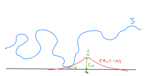
We may assume that the unit normal to is the inner unit normal to , after possibly replacing by . We claim that in each vertical cylinder over a ball of radius contained in there is some point in a distance at most from . Let be small enough that the eigenvalues of are between and in , where . We can choose large so that for
we have outside of and on . If is small and , then outside , hence is a sub-solution to (5) outside . If the claim in the second sentence of the proof was false in the cylinder over some ball for sufficiently large, then we can slide the graph of from below until it touches from one side outside of the cylinder over (see Figure 1), and at the contact point we violate the equation (5).
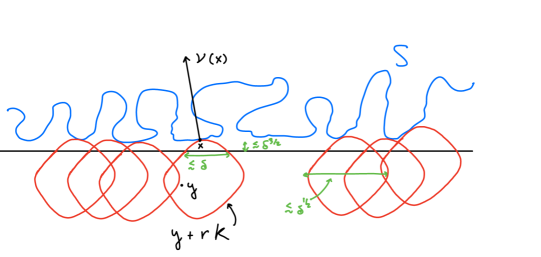
Up to taking smaller we may assume that . Below will denote large constants depending on . We let and we slide copies of centered over points in from below until they touch . By the first step, we can take such that the contact happens at points that are in the cylinder over and in , with upper unit normal lying within of (see Figure 2). Here we are using that is smooth and uniformly convex, hence has interior and exterior tangent spheres of universal radii (depending only on ) at all points on its boundary. The corresponding centers can be found by the relation
Differentiating in gives
Since the second fundamental form of the rescaled Wulff shape at the contact point is (see (3)), we have , whence Since the second term is trace-free we have by the AGM inequality that
Thus, the infinitesimal surface measure of centers is smaller than that of contact points . Since the tangent plane to the surface of contact points at and the surface of centers at is the same, the same inequality holds under projection in the direction. Applying the area formula and recalling that the centers project in the direction to completes the proof.
∎
3. Proof
Before proving Theorem 1.1 we establish some notation. After performing rigid motions, we may assume that , that is tangent to at the origin, and that . We let
There are three possibilities to consider:
-
(A)
(half-space case)
-
(B)
(slab case)
-
(C)
.
We define
| (6) |
where and . It is clear that , and that in cases (B) and (C). To prove Theorem 1.1 it suffices to prove that .
We let denote the graphs of in . When we interpret as the closed half-space in lying above , and we understand similarly when . Finally, we let
so that are the graphs of .
The following is a version of the Hopf lemma, and is reminiscent of a step in the proof of Krylov’s boundary Harnack inequality.
Lemma 3.1.
Assume that is anything in case (A) and nonzero in case (B) or (C). Then contain points that converge as to a point in . The same statement holds with “” replaced by “”.
Proof.
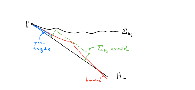
Assume that do not contain points that converge to something in . Then some subsequence avoids a neighborhood of the point in that is unit distance from the origin and orthogonal to . We can find barriers similar to the one in the proof of Lemma 2.1 that are graphs over , bound all from below, and meet at a positive angle (see Figure 3) to conclude that
in for some . Here we used that in cases (B) and (C) to guarantee that the barriers lie below on the boundaries of . From the definition of and the invariance of the right hand side of the above inequality under Lipschitz rescalings, we see that the same inequality holds for in . After taking , we contradict the definition of . After reflecting over , the same argument shows the result with “” replaced by “”.
∎
Proof of Theorem 1.1.
We first treat case (C). If , then by Lemma 3.1 and Lemma 2.1 appropriately rescaled (in fact, just the proof of the first part using barriers) we get that contains points close to that don’t project in the direction to for some large, a contradiction of graphicality (see Figure 4). We conclude that . The assertion that follows from the same argument, after reflection over .
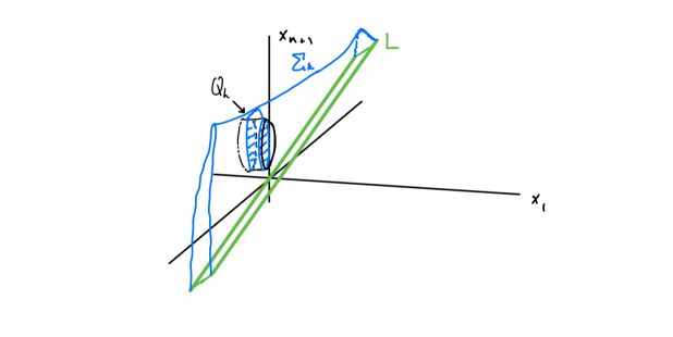
We now turn to case (B). If , then by Lemma 3.1, contain points converging to a point in , thus we contradict the graphicality of over for large. Assume now that . Let be a ball of radius one in that lies above , and let for small to be determined. Lemmas 3.1 and 2.1 (appropriately rescaled) imply that, in , the hypersurfaces contain a sheet of anisotropic area approaching as (see Figure 5). Let and . Then are competitors for in a neighborhood of which for large have anisotropic area bounded above by that of minus plus (the last term coming from the thin sides of the cylinder ). For small we contradict the minimizing property of . We conclude that . The claim that follows in the same way, after reflecting over (and changing the functional accordingly).
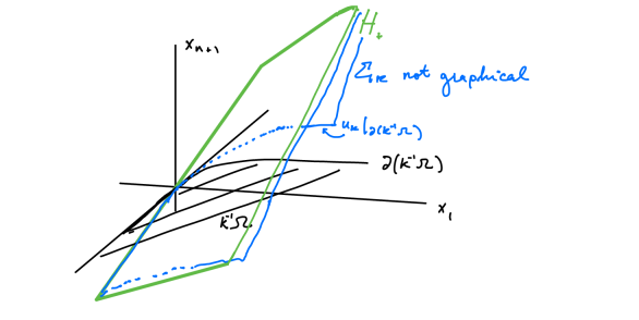
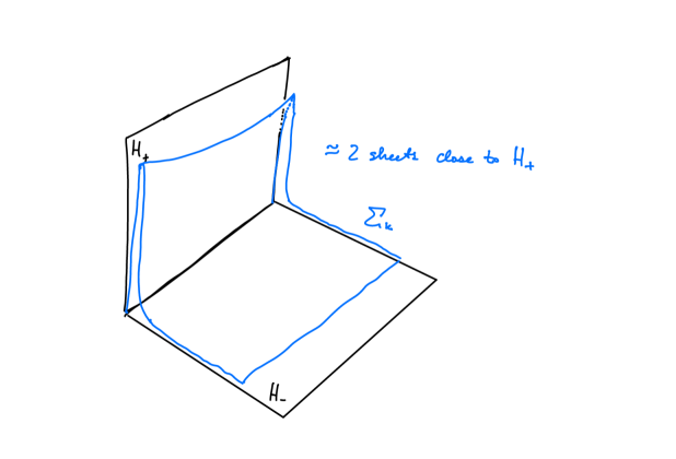
Finally we treat case (A). If and are in and , then Lemma 3.1 and Lemma 2.1 imply that are simultaneously close to in measure for large, which contradicts the graphicality of in the direction. The problem is thus reduced (after possibly reflecting over ) to ruling out the case that . We distinguish two sub-cases. The first is that . Using Lemmas 3.1 and 2.1 near both and we see that in , contain a sheet of anisotropic area approaching , and another portion that projects in the direction to nearly all of . For this one uses that for large, are very close in measure to on regions that get close to (see Figure 6). Thus, the anisotropic area of in is bounded from below by as gets large. Taking and as in case (B) we again contradict minimality for small, since removing removes in but adds at most the anisotropic area of the thin sides and one face of , which is . The alternative is that . In this case Lemmas 3.1 and 2.1 imply that have portions with anisotropic area nearly in and in for large. Using the graphicality of in the direction, we see by the pigeonhole principle that in at least one of , the hypersurface contains another portion that projects in the direction to nearly half of . We may assume that this happens in , after possibly reflecting over . Then the anisotropic area of in is again bounded from below by for large, and we contradict the minimizing property of as in the previous sub-case to complete the proof.
∎
Remark 3.2.
The argument for case (C) in fact shows the linearity of when is any domain in which, outside of a large ball, is contained in a convex cone that is not a half-space.
References
- [1] Allard, W. K. A characterization of the area integrand. Symposia Math. XIV (1974), 429-444.
- [2] Almgren, Jr., F. J.; Schoen, R.; Simon, L. Regularity and singularity estimates on hypersurfaces minimizing elliptic variational integrals. Acta Math. 139 (1977), 217-265.
- [3] Bombieri, E.; De Giorgi, E.; Giusti, E. Minimal cones and the Bernstein problem. Invent. Math. 7 (1969), 243-268.
- [4] De Philippis, G.; De Rosa, A.; Ghiraldin, F. Rectifiability of varifolds with locally bounded first variation with respect to anisotropic surface energies. Comm. Pure Appl. Math. 71 (2018), 1123-1148.
- [5] De Rosa, A.; Tione, R. Regularity for graphs with bounded anisotropic mean curvature. Invent. Math. 230 (2022), 463-507.
- [6] Edelen, N,; Wang, Z. A Bernstein-type theorem for minimal graphs over convex domains. Ann. Inst. H. Poincaré Anal. Non Linéaire 39 (2021), 749-760.
- [7] Figalli, A.; Maggi, F. On the shape of liquid drops and crystals in the small mass regime. Arch. Ration. Mech. Anal. 201 (2011), 143-207.
- [8] Figalli, A.; Maggi, F.; Pratelli, A. A mass transportation approach to quantitative isoperimetric inequalities. Invent. Math. 182 (2010), 167-211.
- [9] Mooney, C. Entire solutions to equations of minimal surface type in six dimensions. J. Eur. Math. Soc. (JEMS) 24 (2022), 4353-4361.
- [10] Mooney, C. The Monge-Ampère equation. Notes, available at https://www.math.uci.edu/mooneycr/MongeAmpere_Notes.pdf
- [11] Mooney, C.; Yang, Y. A proof by foliation that Lawson’s cones are -minimizing. Discrete Contin. Dyn. Syst. 41 (2021), 5291-5302.
- [12] Mooney, C.; Yang, Y. The anisotropic Bernstein problem. Invent. Math., to appear.
- [13] Savin, O. Minimal surfaces and minimizers of the Ginzburg-Landau energy. Contemporary mathematics (American Mathematical Society), v. 528, 2009.
- [14] Simon, L. On some extensions of Bernstein’s theorem. Math. Z. 154 (1977), 265-273.
- [15] Simons, J. Minimal varieties in Riemannian manifolds. Ann. of Math. 88 (1968), 62-105.