Learning finitely correlated states:
stability of the spectral reconstruction

Abstract

We show that marginals of subchains of length $t$ of any finitely correlated translation invariant state on a chain can be learned, in trace distance, with $O(t^{2})$ copies – with an explicit dependence on local dimension, memory dimension and spectral properties of a certain map constructed from the state – and computational complexity polynomial in $t$. The algorithm requires only the estimation of a marginal of a controlled size, in the worst case bounded by a multiple of the minimum bond dimension, from which it reconstructs a translation invariant matrix product operator. In the analysis, a central role is played by the theory of operator systems. A refined error bound can be proven for $C^{*}$-finitely correlated states, which have an operational interpretation in terms of sequential quantum channels applied to the memory system. We can also obtain an analogous error bound for a class of matrix product density operators reconstructible by local marginals. In this case, a linear number of marginals must be estimated, obtaining a sample complexity of $\tilde{O}(t^{3})$. The learning algorithm also works for states that are only close to a finitely correlated state, with the potential of providing competitive algorithms for other interesting families of states.

1 Introduction

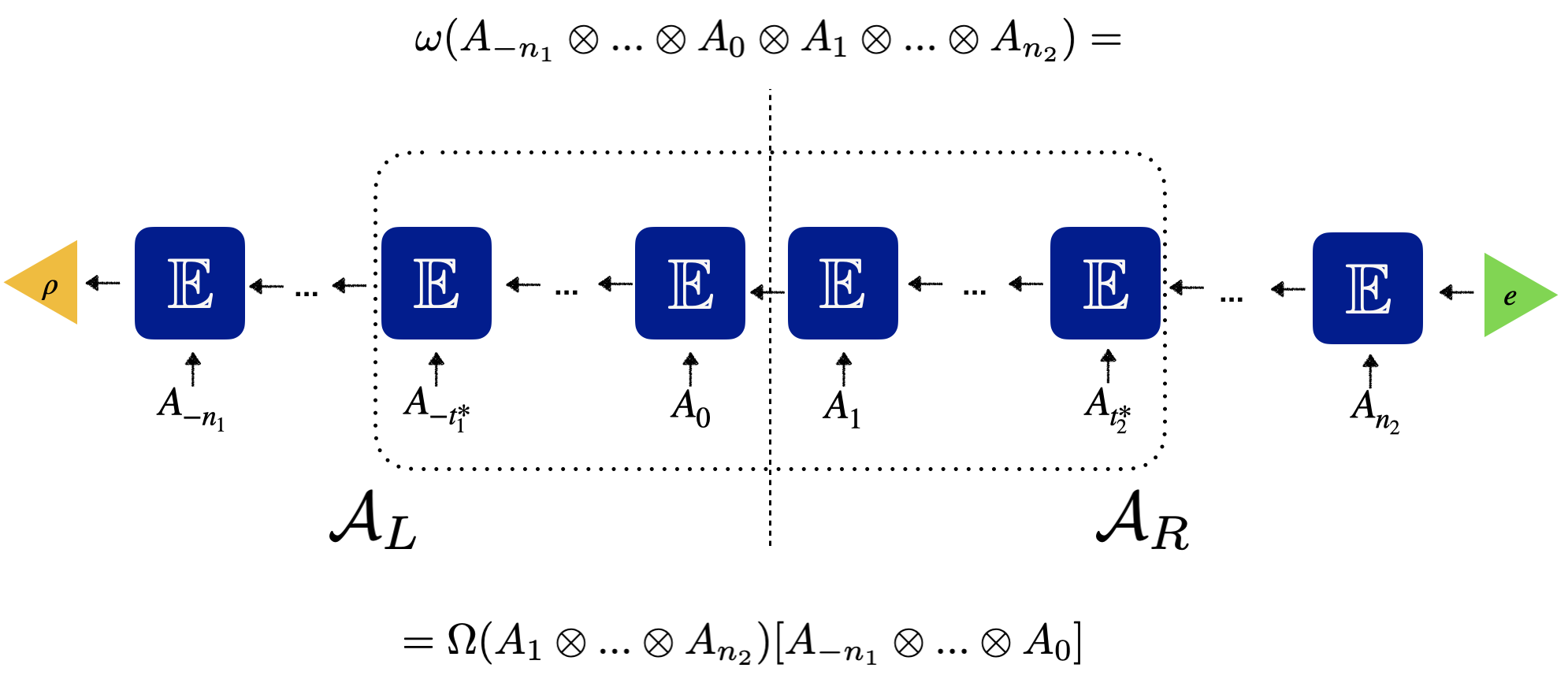
Figure 1: Schematic of a finitely correlated state. The marginal state corresponding the dotted rectangle completely determines the state. An approximate estimate of the marginal can be used to reconstruct an estimate of the state. We bound the error in trace distance of the reconstruction up to a desired size.

Obtaining an approximate description of the state of a quantum system consisting of $t$ qudits (also referred to as spins) to decent accuracy without making any assumptions about its structure infamously requires a number of copies of the state that increases exponentially with $t$. This remains true even if these copies are processed by a fully functional quantum computer capable of executing any measurement allowed by quantum mechanics [1, 2]. Consequently, as the number $t$ of spins grows large, the task of learning a description for an arbitrary state of a many-body system, such as a spin chain, becomes exceedingly challenging. A more manageable scenario arises when one is interested in a measurement procedure that ensures approximate learnability under the hypothesis the state belongs to or is close to some specific class of states characterized by a limited number of parameters. In such a case, the number of required copies can be significantly reduced; this is intuitively related to the fact that now a much smaller number of parameters has to be estimated. Tensor network representations provide a means to identify sets of states with controllable expressiveness, quantified by the number of parameters upon which they depend, and remain one of the most widely studied ansatz class. Likewise, ground and thermal states of local Hamiltonians can be fully described by a polynomial number of parameters. In fact, a substantial body of literature has demonstrated the effectiveness of tensor network states for computing or approximating ground and thermal properties of quantum systems. This effectiveness is supported both by theoretical results [3, 4, 5] and in practice [6]. Furthermore, states generated through consecutive applications of a physical map on a hidden memory system also possess the structure of one-dimensional tensor network states. The expressiveness of these states is constrained by the size of the memory system, as illustrated in Figure 1. These are important classes of states on spin chains that can be generated efficiently on typical quantum systems available in laboratories, including quantum processors.

Tensor network states can be considered also on higher-dimensional lattices. In the present work, however, our focus is on the one-dimensional scenario. In this context, tensor network states go by different names, such as matrix product density operators (MPDO), or matrix product states (MPS) in case they are pure. When there are no constraints on positivity, these tensor network representations are referred to as matrix product operators (MPO) or tensor-trains (TT). Specifically, we are interested in certain classes of tensor network states defined on a chain of length $t$, which can be fully reconstructed by knowing the marginals of a fixed size denoted as $t^{*}$. This property is closely related to the concept of injectivity, as discussed in reference [7]. Notably, a special subset of these states corresponds to the marginals of translation invariant states with finite correlations [8], where the knowledge of a marginal of size $t^{*}$ is sufficient for reconstruction.

Our work rests on the crucial fact, elucidated in [8], that finitely correlated states can be seen as a generalization to the quantum setting of stochastic processes admitting finite dimensional linear models, so-called quasi-realizations [9]. In the classical case, a special subclass of the latter go by the name of hidden Markov models [10, 9] (also known as positive realizations). In the quantum case, the natural analogue of hidden Markov models are the aforementioned description of states generated by consecutive applications of a quantum channel to a memory system. We call these models $C^{*}$-realizations. Note however that the class of finite dimensional models is not completely exhausted by finite dimensional $C^{*}$-models, as a recent result by some of the present authors shows [11].

In the classical literature on stochastic processes, learning guarantees for hidden Markov models have been established: a series of works starting with [12] has shown that an estimate of the relevant marginal at precision $\epsilon$ gives rise to a reconstruction of the process which has an error in total variation distance that can be bounded as $O(\operatorname{poly}(t,\epsilon^{-1},m))$ with $t$ being the timespan considered, and $m$ the size of the hidden memory. This in turn implies a rigorous sample complexity bound which scales quadratically in the system size. In the quantum setting, reconstruction algorithms using a similar idea have been proposed, already in the non-translation invariant setting [13, 14] and their practicality and efficiency has been demonstrated with experiments [15]. Moreover, when the reconstruction can be achieved from the knowledge of local marginals of sufficiently small size, local measurements suffice and the quantum complexity of the algorithm is much more tractable than in the general case. However, until the present work, a thorough analysis of the sample complexity of the reconstruction algorithm in the quantum case appeared to be lacking [16]. Here, we precisely propose to fill this gap. Our algorithm and proof strategy build on the classical case, with however important differences due to the presence of entangled observables, and the use of the appropriate operator norms. In fact, our analysis fully exploits the fact that finitely correlated states naturally define an operator system on which one can speak of completely positive maps. This allows us to treat not only the case of states generated by repeated quantum measurements, but also models for which no explanation with finite-dimensional quantum memory exist. Notably, this even provides error bounds for learning classical states that were not previously available. Moreover, the analysis can be generalized to the non-homogeneous case, which is of notable interest since it can address learning of physically motivated states in finite-size systems.

1.1 Background and related work

As already mentioned, our approach draws inspiration from the literature on hidden Markov models, specifically focusing on what are commonly referred to as “spectral algorithms”. These algorithms are designed to reconstruct a linear model that explains a stochastic process through the estimation of marginals and matrix algebra operations. They aim to overcome the limitations of maximum likelihood approaches, which often lack rigorous convergence guarantees. Spectral algorithms have been applied in more general graphical models as well [17]. The core idea behind these algorithms is to view the probabilities associated with concatenated words as the matrix elements of a mapping between the right segment of the chain and linear functionals on the left segment of the chain. It is assumed that this mapping can be determined by its action on a finite block of the chain. Essentially, these algorithms construct a linear model where the memory system comprises the functionals determined in this manner, and the dynamics are also governed by these functionals. One challenge in ensuring the accuracy of these algorithms lies in their reliance on matrix inversion, which makes them sensitive to small singular values. In a prior study [12], it was demonstrated that the spectral algorithm provides an error bound in terms of total variation distance, assuming that the underlying process closely resembles a hidden Markov model and that certain matrices constructed from hidden Markov model parameters have controlled singular values. This established a learning guarantee akin to PAC (Probably Approximately Correct) learning, which becomes more tractable by narrowing the class of target processes. Subsequent works, among them [18] and [19], relaxed some of the assumptions made in [12], such as the requirement of reconstructing from marginals of size three and invertibility assumptions on the so-called observation matrix (see Section 2.2.1). Nevertheless, a key premise in these works is indeed the existence of an approximating hidden Markov model. To the best of our knowledge, no error bound in total variation distance has been derived for general models (as discussed in [19] and [20]). Notably, there does not even seem to exist an error bound for stochastic processes generated by hidden quantum Markov models, which have been proven to be more expressive than classical ones [21, 22], although they are not as expressive as the most general class of processes one could consider [11]. As a result, the idea of investigating spectral algorithms in the context of hidden quantum Markov models was suggested in [23].

In the quantum information literature, a reconstruction method related to the spectral algorithm we propose is the direct tomography algorithm in [13], which learns a circuit preparing an MPS by knowledge of marginals of sufficiently large size. For general states, the state reconstruction scheme in [14] from the exact knowledge of the marginals, is analogous to the one we present, but is lacking an error bound on the precision of the reconstruction. Moreover, our algorithm uses a slightly different prescription for the reconstruction from empirical data. Note that these algorithms were directly proposed in the non-translation-invariant (non-homogeneous) setting, in contrast to the classical ones. In terms of our error analysis, there is no substantial difference between these two cases except for the fact that, in the non-homogeneous case, one is required to learn several marginal blocks of the state instead of a single arbitrary one. The robustness of the matrix reconstruction in the bipartite case was already discussed in [14] and investigated in more depth in [24], where the authors obtained a bound on the accuracy in terms of the operator norm. However, an error bound in trace distance was not explicitly stated, and it is not clear how to adapt their analysis to get a bound for a chain as opposed to a bipartite state. To perform a similar step in our setting, we instead adapt the analysis carried by [12, 18, 19] to the quantum case. Learning the marginals themselves can be done in several ways, and we take the necessary size of the marginals as a parameter of our class. In the translation invariant case, this size is at most of the order of the minimal dimension of the memory system (bond dimension), while in the non-homogenous case it can be arbitrarily large. That being said, in addition to the use of strictly local measurements to learn the marginals, one can use other methods such as constrained maximum likelihood learning algorithms based on measurement statistics. A very recent result [25] in that direction provides a bound in Hilbert-Schmidt norm for the error in the reconstruction of the state which is polynomial in the size and requires global (in fact Haar random), yet independent, single-copy measurements. It is unclear to us whether this bound directly leads to a good error bound in trace distance. Instead, we use it as a means to learn the marginals with an error in Hilbert-Schmidt distance, which serves our needs adequately as we will show in Section 4.

1.2 Main results

In the following, $\mathcal{A}$ is a generic finite-dimensional $C^{*}$-algebra, but it is sufficient to think about it as embedded in a matrix algebra of $d_{\mathcal{A}}\times d_{\mathcal{A}}$ complex matrices, which is associated to qudit observables. We consider a translation invariant state $\omega$ on an infinite one-dimensional chain, where the algebra associated to site $i\in\mathbb{N}$ is denoted as $\mathcal{A}_{i}=\mathcal{A}$ and the algebra associated to the spins from $a$ to $b$ is denoted as $\mathcal{A}_{[a,b]}$. We are interested in learning the marginal on $\mathcal{A}_{[1,t]}$, which we denote as $\omega_{t}$.

Definition 1.1.

A realization of a translation invariant state $\omega$ is a quadruple $(V,e,\mathbb{E},\rho)$, where $V$ is a finite-dimensional vector space, $\mathbb{E}$ a linear map $\mathbb{E}:\mathcal{A}\ni A\mapsto\mathbb{E}_{A}\in\mathrm{Hom}(V)$, $e$ an element of $V$, and $\rho$ a linear functional in $V^{*}$, such that

$$\omega(A_{1}\otimes\cdots\otimes A_{n})=\rho\mathbb{E}_{A_{1}}\cdots\mathbb{E}_{A_{n}}(e),$$ (1)

and

$$\rho\circ\mathbb{E}_{\mathds{1}}=\rho,\qquad\mathbb{E}_{\mathds{1}}(e)=e.$$ (2)

A translation invariant state $\omega$ admitting a realization is called a finitely correlated state.

Dividing the chain in two parts, we can recognize a right chain algebra $\mathcal{A}_{R}$ associated to all the sites with index $i>0$, and a left chain algebra $\mathcal{A}_{L}$ associated to sites with index $i\leq 0$. Through the state $\omega$ one can define a linear map $\Omega$ from $\mathcal{A}_{R}$ to linear functionals on $\mathcal{A}_{L}$, as $\Omega(A_{r})[A_{l}]:=\omega(A_{l}\otimes A_{r})$. One can show that this map has finite rank, and that there exists a finite subchain, from site $-t_{1}^{*}$ to $t_{2}^{*}$, such that the restriction of the map $\Omega$ to this chain, sending $A_{[1,t_{2}^{*}]}$ to functionals on $A_{[-t_{1}^{*},0]}$ completely determines $\Omega$, see Corollary D.2. The rank of $\Omega$ gives the minimal dimension $m$ of a realization of $\omega$. The smallest nonzero singular value of the restriction of $\Omega$ to the subchain is denoted as $\sigma_{m}(\Omega)$. Moreover, the minimal size of the subchain can be taken to be less than $2m+1$.

If the realization is such that $V$ is the space of $d_{\mathcal{B}}\times d_{\mathcal{B}}$ matrices (or indeed any finite-dimensional $C^{*}$-algebra), $\mathbb{E}$ is completely positive and unital, $e$ is the $d_{\mathcal{B}}$-dimensional identity matrix and $\rho$ is a density matrix in $d_{\mathcal{B}}\times d_{\mathcal{B}}$, then the realization is said to be a $C^{*}$-realization. Then, $C^{*}$-finitely correlated states are those admitting a $C^{*}$-realization. Operationally, this means that they can be obtained by sequential application of a quantum channel which has a memory system of dimension $d_{\mathcal{B}}$ as input and as output the memory system itself and a system of dimension $d_{\mathcal{A}}$ (this channel would be the adjoint of the map $\mathbb{E}$).

Beyond $C^{*}$-finitely correlated states, one can use the fact that it is always possible to give the image of $\Omega$ an operator system structure for which $\mathbb{E}$ is completely positive [26], thus interpreting finitely correlated states as states obtained by sequential applications of a physical map to a memory system obeying some general probabilistic theory.

We obtain the following Theorems, based on the analysis of Algorithm 1.

Theorem 1.2.

Let $\omega$ be a finitely correlated state of rank $m$, with associated map $\Omega$. There exists an algorithm which takes as input $n$ copies of $\omega$, an integer $s$ and a threshold $\eta$ such that it makes measurements on marginals of size $s$ and it outputs an estimate $\hat{\omega}_{t}$ (not necessarily positive-semidefinite) such that, with high probability

$$d_{\mathrm{Tr}}(\hat{\omega}_{t},\omega_{t})\leq\epsilon$$ (3)

whenever $s\geq\max\{t_{2}^{*},t_{1}^{*}+1\}$, $\sigma_{m}(\Omega)/2\geq\eta\geq 2\varepsilon$ with $\varepsilon=\frac{\epsilon\sigma^{3}_{m}(\Omega)}{20tm\sqrt{d_{\mathcal{A}}}}$, and $n$ larger than the number of copies of $\omega_{2s},\omega_{2s+1}$ necessary for learning $\omega_{2s},\omega_{2s+1}$ in Hilbert-Schmidt distance at precision $\varepsilon$.

Theorem 1.3.

Let $\omega$ be a $C^{*}$-finitely correlated state with memory system $\mathbb{M}_{d_{\mathcal{B}}}$ and associated map $\Omega$. There exists an algorithm which takes as input $n$ copies of $\omega$, an integer $s$ and a threshold $\eta$ such that it makes measurements on marginals of size $s$ and it outputs an estimate $\hat{\omega}_{t}$ (not necessarily positive-semidefinite) such that, with high probability

$$d_{\mathrm{Tr}}(\hat{\omega}_{t},\omega_{t})\leq\epsilon$$ (4)

whenever $s\geq\max\{t_{2}^{*},t_{1}^{*}+1\}$, $\sigma_{m}(\Omega)/2\geq\eta\geq 2\varepsilon$ with $\varepsilon=\frac{\epsilon\sigma^{3}_{m}(\Omega)}{20td_{B}\sqrt{d_{\mathcal{A}}}}$, and $n$ larger than the number of copies of $\omega_{2s}$ and $\omega_{2s+1}$ necessary for learning $\omega_{2s},\omega_{2s+1}$ in Hilbert-Schmidt distance at precision $\varepsilon$.

For the proofs, see Theorem 4.6 in Section 4 and Theorem 4.9 in Section 4.4.

Remark 1.4.

In the following we set $d_{\mathcal{B}}=+\infty$ if a finitely correlated state does not admit a finite dimensional $C^{*}$-realization. With local measurements, one can set a number of copies of $\omega_{2s+1}$ equal to $n=O\left(\frac{d_{A}^{2s}}{\varepsilon^{2}}\right)$ (see the analysis of the result by [27] in [2]), obtaining

$$n=O\left(\frac{t^{2}\min(m^{2},d_{\mathcal{B}}^{2})^{2}d_{\mathcal{A}}^{2s+1}}{\epsilon^{2}\sigma_{m}(\Omega)^{6}}\right).$$ (5)

With global but single-copy measurements, one can set $n=\tilde{O}\left(\frac{s^{3}d^{2}_{\mathcal{A}}m^{2}}{\varepsilon^{2}}\right)$ [25], so that

$$n=\tilde{O}\left(\frac{s^{3}t^{2}m^{2}\min(m^{2},d_{\mathcal{B}}^{2})d_{\mathcal{A}}^{3}}{\epsilon^{2}\sigma_{m}(\Omega)^{6}}\right).$$ (6)

The proof is based on the following ideas. First, there exists a way to obtain a realization from observable quantities, meaning expectation values of observables. One can then obtain a guess for the realization via empirical estimation of these expectation values. The realization is not unique, and the idea of [12] is to bound the error in the reconstruction comparing the empirical estimate with an exact realization which depends on the empirical estimate itself. Our analysis shows that this is possible in full generality in the quantum case too. In addition, we can put an operator system structure for which the map appearing in this realization is completely positive and unital. We then obtain the bound on the trace distance as a function of suitable expressions involving the accuracy of the estimations of the marginals, via a recursive analysis on the error accumulation of the reconstruction based on (i) the completely positive, unital map generating the state is contractive with respect to the operator system norm; and on (ii) submultiplicativity of completely bounded operator norms. We can then reduce the remaining quantities to Hilbert-Schmidt error of the estimates of the marginal, by using the theory of completely bounded maps, in particular the property that the completely bounded norm of finite rank maps can be controlled by the operator norm, and that for maps to matrices we can compute it by doing so for a single, large enough amplification; we then use an adaptation of the matrix perturbation analysis of [12, 18, 19], obtaining the final result.

We conclude this introduction with some comments on the extensions of the main result, which we further discuss in the appropriate sections below:

• In the general case, while the error propagation bound continues to have the correct form, expressing the error parameters in terms of the Hilbert-Schmidt error of the marginal estimates requires defining a suitable ‘Hilbert-Schmidt norm’ $\|\cdot\|_{\Omega}$, constructed from the map $\Omega$, and giving explicit constants in the equivalence with the order norm $\|\cdot\|_{e}$. We can in fact obtain $\sigma_{m}(\Omega)\|\cdot\|_{e_{n}}\leq\|\cdot\|_{n,\Omega}\leq\sqrt{n}\|\cdot\|_{e_{n}}$ for the norms on the matrix amplifications, whose proof could be of independent interest, as it applies to general bipartite states. The proof of these inequalities is based on the theory of operator systems. See Section 3.

• The non-homogeneous case can be addressed with essentially the same proof. We provide a reconstruction algorithm in our notation, and argue that the error propagation bound has the same form of the translation invariant case. Of course, one needs that all the estimations of the marginals are $\varepsilon$ accurate. If each marginal is estimated in an independent run of measurements, this increases the number of copies by a factor linear in the size of the state. See Section 5.

• We also propose a new path for learning one-dimensional Gibbs states in terms of their approximations by matrix product operators. Indeed, in [28] the authors constructed depth-two dissipative quasi-local circuits whose $C^{*}$-finitely correlated outputs approximate such states in trace distance. Combining this fact with our robust learning algorithm (see Proposition 6.1) we achieve a polynomial sample complexity for the task of learning the reduced states of a Gibbs state at any positive temperature, similarly to that of [29]. However, the degree of the polynomial we achieve with our algorithm in its current state depends on the temperature, and we leave the question of optimizing our procedure to future work. See Section 6.

Algorithm 1 LearnFCS

1:Input: State $\omega^{\otimes n}$, $s\in\mathbb{N}$, $\eta\in\mathbb{R}$, basis $\mathcal{B}_{\mathcal{A}}=\{Z_{i}\}_{i=1}^{d_{\mathcal{A}}},\mathcal{B}_{\mathcal{A}_{L}}=\{Y_{i}\}_{i=1}^{d^{s}_{\mathcal{A}}},\mathcal{B}_{\mathcal{A}_{R}}=\{X_{i}\}_{i=1}^{d^{s}_{\mathcal{A}}}$

2:Use Tomography$(\omega^{\otimes n},s)$ and produce empirical estimates:

• $\hat{\Omega}(X_{i})[Y_{j}]=\hat{\omega}_{2s}(Y_{j}\otimes X_{i})$

• $\hat{\Omega}_{Z_{k}}(X_{i})[Y_{j}]=\hat{\omega}_{2s+1}(Y_{j}\otimes Z_{k}\otimes X_{i})$

for all $Z_{k}\in\mathcal{B}_{\mathcal{A}}$, $Y_{j}\in\mathcal{B}_{\mathcal{A}_{L}}$ and $X_{i}\in\mathcal{B}_{\mathcal{A}_{R}}$.

3:Compute the SVD of $\hat{\Omega}=\hat{U}\hat{D}\hat{W}^{\intercal}$ and truncate the columns of $\hat{U}$ such that we keep the columns corresponding the singular values $\sigma_{i}(\hat{\Omega})\geq\eta$.

4:Compute the estimated realization operators:

• $\hat{e}={\hat{U}}^{\intercal}\hat{\Omega}(\mathds{1})$

• $\hat{\rho}=\tau\hat{U}$

• $\hat{\mathbb{K}}_{Z_{i}}={\hat{U}}^{\intercal}(\hat{\Omega}_{Z_{i}})({\hat{U}}^{\intercal}\hat{\Omega})^{+}$ for all basis elements $Z_{i}\in\mathcal{B}_{\mathcal{A}}$.

5:Reconstruct $\hat{\omega}_{t}$ using

$$\hat{\omega}_{t}(Z_{1}\otimes\cdots\otimes Z_{t}):=\hat{\rho}\hat{\mathbb{K}}_{Z_{1}}\cdots\hat{\mathbb{K}}_{Z_{t}}\hat{e}$$

for all $Z_{i}\in\mathcal{B}_{\mathcal{A}}$.

Figure 2: Finitely correlated state learning algorithm. Tomography$(\omega^{\otimes n},s)$ is any subroutine that takes input $n$ copies of the state $w$ and learns the marginals $\hat{\omega}_{2s}$ and $\hat{\omega}_{2s+1}$ on a subset of the chain of length respectively $2s$ and $2s+1$.

1.3 Outline

The rest of the paper is structured as follows. In Section 2 we set up the notation and present the objects that we use in the analysis, such as several particular realizations of a fixed state and how they are connected to each other. In Section 3 we discuss the operator systems associated with realizations. In Section 4 we show the main result for general states, while in Section 4.4 we treat the special case of $C^{*}$-finitely correlated states. In Section 5 we extend the arguments to the non-translation invariant case, for states on a finite chain. In Section 6 we consider how the algorithm can be used to learn states which are only close to finitely correlated, including Gibbs states. In Section 7 we report some numerical experiments.

2 Preliminaries

2.1 Notation

In the following we think of states as non-negative linear functionals from a $C^{*}$-algebra to $\mathbb{C}$. For finite dimensional systems, we can simply think of a density matrix $\rho\in\mathbb{M}_{n}$ as a functional on $\mathbb{M}_{n}$, $\rho(X)=\operatorname{Tr}[\rho X]$. Let us fix the notations for states on an infinite chain following [8]. We consider states on an infinite chain with sites labelled by $n\in\mathbb{Z}$, where to each site $n$ a finite dimensional $C^{*}$-algebra $\mathcal{A}_{n}\equiv\mathcal{A}$ is associated. Without loss of generality, $\mathcal{A}$ can be embedded into the algebra of $d_{\mathcal{A}}\times d_{\mathcal{A}}$ matrices $\mathbb{M}_{d_{\mathcal{A}}}$. For each finite subset $X$ of $\mathbb{Z}$ we can define an algebra $\mathcal{A}_{X}:=\bigotimes_{n\in X}\mathcal{A}_{n}$. The algebra of infinite subsets is defined through the inductive limit, with the identifications $\mathcal{A}_{X_{1}}\equiv\mathcal{A}_{X_{1}}\otimes\mathds{1}_{X_{2}\setminus X_{1}}$ for $X_{1}\subseteq X_{2}$ finite subsets. The chain algebra $\mathcal{A}_{\mathbb{Z}}$ is defined in this way, for example, as the inductive limit for sets $[-n,n]:=\{-n,\dots,n\}$. The right chain algebra $\mathcal{A}_{R}$ is defined as the inductive limit of $\mathcal{A}_{[1,n]}$, and the left chain algebra $\mathcal{A}_{L}$ is defined as the inductive limit of $\mathcal{A}_{[-n,0]}$. The translation operators $\alpha_{r}$ act on the algebra by sending $\mathcal{A}_{X}$ into $\mathcal{A}_{X+r}$. We denote the set of translation invariant states by $\mathcal{T}$.

For linear maps $L:V_{1}\rightarrow V_{2}$ and $M:V_{2}\rightarrow V_{3}$ we write the composition of $M$ and $L$ simply as $ML$. The identity map on a vector space $V$ is denoted as $\mathrm{id}_{V}$, the identity element of a $C^{*}$-algebra $\mathcal{A}$ is denoted as $\mathds{1}_{\mathcal{A}}$. Given a linear map $\mathbb{E}:\mathcal{A}\ni A\mapsto\mathbb{E}_{A}\in\mathrm{Hom}(V)$, we use the notation $\mathbb{E}^{t}:\mathcal{A}^{\otimes t}\ni A\mapsto\mathbb{E}_{A}\in\mathrm{Hom}(V)$ for the linear map that acts on tensor product vectors as $\mathbb{E}^{t}_{X_{1}\otimes\cdots\otimes X_{t}}=\mathbb{E}_{X_{1}}\cdots\mathbb{E}_{X_{t}}$. Similarly, given a linear map $\mathbb{E}:\mathcal{A}\otimes V\rightarrow V$, we use the notation $\mathbb{E}^{t}:\mathcal{A}^{\otimes t}\otimes V\rightarrow V$ for the linear map that acts on product vectors as $\mathbb{E}^{t}(X_{1}\otimes\cdots\otimes X_{t}\otimes x)=\mathbb{E}_{X_{1}}\cdots\mathbb{E}_{X_{t}}(x)$.

Additionally, we use the following notation for linear maps. We denote by $\|T\|_{p}=(\operatorname{Tr}[(T^{\dagger}T)^{{p}/{2}}])^{1/p}$ the Schatten $p$-norm for $T:H_{1}\rightarrow H_{2}$ being a linear map between finite dimensional Hilbert spaces $H_{1},\,H_{2}$, where $T^{\dagger}$ is the adjoint map (we also use the notation $U^{\intercal}$ if we deal with maps between real vector spaces). The singular values of $T$ are denoted and ordered as $\sigma_{1}(T)\geq\sigma_{2}(T)\geq\dots\geq\sigma_{r}(T)$, so that $\|T\|_{p}=\left(\sum_{i=1}^{r}\sigma_{i}(T)^{p}\right)^{1/p}$. We denote by $T^{+}$ the Moore-Penrose pseudoinverse of $T$. For a map $L:B_{1}\rightarrow B_{2}$, where $B_{1}$ and $B_{2}$ are spaces of finite dimensional linear maps equipped with Schatten norms, we have $\|L\|_{p\rightarrow p}:=\sup_{X\in B_{1},\|X\|_{p}\leq 1}\|L(X)\|_{p}$, and $\|L\|_{p\rightarrow p,cb}:=\sup_{d\in\mathbb{N}}\sup_{X\in\mathbb{M}_{d}\otimes B_{1},\|X\|_{p}\leq 1}\|(\mathrm{id}_{\mathbb{M}_{d}}\otimes L)(X)\|_{p}$. By slight abuse of notations, for $p\in[1,\infty]$, we will also denote by $\|\cdot\|_{p}$ the usual $\ell_{p}$ norm on $\mathbb{R}^{m}$, as well as the $p$-norm of linear functionals: given a functional $\varphi$ on a (matrix) space $\mathcal{C}$, $\|\varphi\|_{p}:=\sup_{\|X\|_{p^{\prime}}\leq 1}|\varphi(X)|$, where $1/p^{\prime}+1/p=1$. For $p=2$, this is also equal to $\|\varphi\|_{2}=(\sum_{i}|\varphi(X_{i})|^{2})^{1/2}$ for some orthonormal basis $\{X_{i}\}$ of $\mathcal{C}$.

2.2 Finitely correlated states

A subclass of translation invariant states are finitely correlated states, which admit the following description.

Definition 2.1.

A (linear) realization of a translation invariant state $\omega$ is a quadruple $(V,e,\mathbb{E},\rho)$, where $V$ is a finite-dimensional vector space serving as a memory, $\mathbb{E}$ a linear map $\mathbb{E}:A\in\mathcal{A}\rightarrow\mathbb{E}_{A}\in\mathrm{Hom}(V)$, $e$ an element of $V$, and $\rho$ a linear functional in $V^{*}$, such that

$$\omega(A_{1}\otimes\cdots\otimes A_{n})=\rho\mathbb{E}_{A_{1}}\cdots\mathbb{E}_{A_{n}}(e),$$ (7)

and

$$\rho\mathbb{E}_{\mathds{1}}=\rho\qquad\mathbb{E}_{\mathds{1}}(e)=e.$$ (8)

A translation invariant state $\omega$ admitting a realization is called a finitely correlated state.

The following characterization holds, from Proposition 2.1 of [8].

Proposition 2.2.

Let $\mathcal{A}$ be a $C^{*}$-algebra with unit, and let $\omega$ be a translation invariant state on the chain algebra $\mathcal{A}_{\mathbb{Z}}$. Then the following are equivalent:

• The set of functionals $\Psi_{X}:\mathcal{A}_{L}\rightarrow\mathbb{C}$ of the form

  $$\Psi_{X}(A_{-n}\otimes\cdots\otimes A_{0})=\omega(A_{-n}\otimes\cdots\otimes A_{0}\otimes X)$$ (9)

  with $X\in\mathcal{A}_{R}$ and $n\in\mathbb{N}$ generates a finite-dimensional linear subspace in the dual of $\mathcal{A}_{L}$, of dimension $m$, say.

• There exists a realization $(V,e,\mathbb{E},\rho)$ of $\omega$.

Moreover, the minimal dimension of $V$ is $m$.

Furthermore, also as part of [8, Prop. 2.1] we have

Proposition 2.3.

Realizations of minimal dimension, called regular realizations, are determined up to linear isomorphisms: if $(V,e,\mathbb{E},\rho)$ and $(V^{\prime},e^{\prime},\mathbb{E}^{\prime},\rho^{\prime})$ are two regular realizations of $\omega$, then $V$ and $V^{\prime}$ are isomorphic via a unique invertible linear map $M:V\rightarrow V^{\prime}$, such that $e^{\prime}=Me$, $\rho^{\prime}=\rho M^{-1}$, $\mathbb{E}^{\prime}_{A}=M\mathbb{E}_{A}M^{-1}$.

In the proof of the above statements, it is used that a realization of minimal dimension can be obtained as a quotient realization of any realization. Note, that if $\tilde{W}\subset V^{*}$ is a set of linear functionals, we denote the subspace on which they all vanish simultaneously by $\tilde{W}^{\perp}$ (that is, $\tilde{W}^{\perp}$ is just the intersection of their kernels).

Proposition 2.4.

Let $(V,e,\mathbb{E},\rho)$ be a realization of a translation invariant state $\omega$, whose minimal realizations are of dimension $m$. Define $W=\{\mathbb{E}^{k}_{A}e\ |\ A\in\mathcal{A}_{[1,k]},k\in\mathbb{N}_{>0}\}$, and $\tilde{W}=\{\rho\mathbb{E}^{k}_{A}\ |\ A\in\mathcal{A}_{[1-k,0]},k\in\mathbb{N}_{>0}\}$, set $V^{\prime}:=W/({W\cap\tilde{W}^{\perp}})$ and $L:=W\rightarrow V^{\prime}$ the canonical projection. Then $\dim{V^{\prime}}=m$, and there exists a (thus regular) realization $(V^{\prime},e^{\prime},\mathbb{K}^{\prime},\rho^{\prime})$ such that, for the restrictions $\mathbb{E}_{A}|_{W}$ and $\rho|_{W}$ to $W$ we have:

$$\mathbb{K}^{\prime}_{A}L =L\mathbb{E}_{A}|_{W},$$ (10)

$$\rho^{\prime}L =\rho|_{W},$$ (11)

$$e^{\prime} =Le.$$ (12)

2.2.1 Observable regular realization

The proof of Proposition 2.2 gives also a way to construct a realization from the knowledge of a marginal of the state on a finite subset of the chain. We call this realization observable regular realization, as it is expressed only in terms of quantities which can be estimated from experiments.

Let us select two finite-dimensional unital subalgebras $\mathcal{C}_{R}\subseteq\mathcal{A}_{R}$ and $\mathcal{C}_{L}\subseteq\mathcal{A}_{L}$ such that the vector space generated by functionals $\Psi_{X}:\mathcal{C}_{L}\rightarrow\mathbb{C}$ of the form

$$\Psi_{X}(Y):=\omega(Y\otimes X),$$ (13)

with $X\in\mathcal{C}_{R}$, has dimension $m$. We call this vector space $V$, which can be thought of as a subspace of ${\mathcal{A}_{\Lambda}^{*}\cong\mathcal{A}_{\Lambda}}$, for some finite subset $\Lambda$ of the chain, say $\Lambda=[1,t^{*}]$ for some $t^{*}\leq m$ (see Appendix D), and define $L$ to be a projection from $\mathcal{A}_{\Lambda}^{*}$ to $V$.

We can thus define the map $\mathbb{E}:\mathcal{A}\ni A\mapsto\mathbb{E}_{A}\in\mathrm{Hom}(\mathcal{A}^{*}_{\Lambda})$ as

$$\mathbb{E}_{A}(\Psi_{X}):=\Psi_{A\otimes X},$$ (14)

and by setting $\mathbb{E}_{A}$ to be $0$ on the orthogonal complement of $V$. We define the functional $\tau\in\mathcal{A}_{\Lambda}^{**}$ as

$$\tau(Y)=Y(\mathds{1}),\,\,\forall\,Y\in\mathcal{A}_{\Lambda}^{*}\,.$$ (15)

Note that identifying $\mathcal{A}_{\Lambda}^{*}$ with $\mathcal{A}_{\Lambda}$ through the Hilbert-Schmidt inner product, $\tau$ acts as the trace functional.

Define the maps $\Omega:\mathcal{C}_{R}\rightarrow\mathcal{C}_{L}^{*}$ and $\Omega_{(\cdot)}:\mathcal{A}\otimes\mathcal{C}_{R}\rightarrow\mathcal{C}_{L}^{*}$ through

$$\Omega(X)[Y] :=\omega(Y\otimes X)$$ (16)

$$\Omega_{A}(X)[Y] :=\omega(Y\otimes A\otimes X),$$ (17)

where $\Omega_{(\cdot)}$ is extended linearly to all of $\mathcal{A}\otimes\mathcal{C}_{R}$. Fix a self-adjoint basis $\{X_{i}\}_{i=1}^{m_{1}}$ of $\mathcal{C}_{R}$, such that $\operatorname{Tr}[X_{i}X_{j}]=\delta_{ij}$, and a self-adjoint basis $\{Y_{i}\}_{i=1}^{m_{2}}$ of $\mathcal{C}_{L}$, such that $\operatorname{Tr}[Y_{i}Y_{j}]=\delta_{ij}$. By singular value decomposition, we can write

$$\Omega=UDO,$$ (18)

with $D$ diagonal in $\mathbb{R}_{\geq 0}^{m\times m}$, $U:\mathbb{C}^{m}\rightarrow\mathcal{C}_{L}^{*}$ and $O:\mathcal{C}_{R}\rightarrow\mathbb{C}^{m}$ partial isometries, with real entries in the chosen basis and satisfying $U^{\intercal}U=OO^{\intercal}=\mathds{1}_{\mathbb{C}^{m}}$.

Proposition 2.5 (Observable regular realization).

$(\mathbb{C}^{m},e,\mathbb{K},\rho)$ is a regular realization, where

$$e :=U^{\intercal}\Omega(\mathds{1}),$$ (19)

$$\rho :=\tau U=\tau\Omega(U^{\intercal}\Omega)^{+},$$ (20)

$$\mathbb{K}_{A} :=U^{\intercal}\Omega_{A}(U^{\intercal}\Omega)^{+}.$$ (21)

Proof.

We have that

$${\mathbb{E}_{A}\Omega(X)=\mathbb{E}_{A}\Psi_{X}=\Psi_{A\otimes X}=\Omega_{A}}(X)\,,$$ (22)

and therefore

$$\mathbb{E}_{A}U=\Omega_{A}(DO)^{+}=\Omega_{A}(U^{\intercal}\Omega)^{+}\,,$$ (23)

where we have also used that $U^{\intercal}U=\mathds{1}_{\mathbb{C}^{m}}$ so that $U^{\intercal}\Omega=DO$. Indeed we have

$$\mathbb{K}_{A}U^{\intercal} =U^{\intercal}\Omega_{A}(U^{\intercal}\Omega)^{+}U^{\intercal}=U^{\intercal}\mathbb{E}_{A}UU^{\intercal},$$ (24)

which lets us conclude $\mathbb{K}_{A}U^{\intercal}=U^{\intercal}\mathbb{E}_{A}$, since $P_{U}=UU^{\intercal}$ is the projector on the space identified with $V$ in $\mathcal{A}^{*}_{\Lambda}$, and both $U^{\intercal}$ and $\mathbb{E}_{A}$ are zero on the orthogonal complement of $V$ (so in particular $\mathbb{E}_{A}P_{U}=\mathbb{E}_{A}$). Hence, we have proved that

$$\rho\mathbb{K}_{A_{n}}\dots\mathbb{K}_{A_{1}}e=\tau P_{U}\mathbb{E}_{A_{n}}P_{U}\dots\mathbb{E}_{A_{1}}P_{U}\Psi_{\mathds{1}}=\tau\mathbb{E}_{A_{n}}\dots\mathbb{E}_{A_{1}}\Psi_{\mathds{1}}\,,$$

and therefore $(\mathbb{C}^{m},e,\mathbb{K},\rho)$ is a regular realization of $\omega$. ∎

Let $(V,u,\mathbb{E},\sigma)$ be any realization and $(V^{\prime},e^{\prime},\mathbb{K}^{\prime},\rho^{\prime})$ its quotient realization. Since $(V^{\prime},e^{\prime},\mathbb{K}^{\prime},\rho^{\prime})$ and the observable realization $(\mathbb{C}^{m},e,\mathbb{K},\rho)$ constructed in Proposition 2.5 are both regular, there is a unique invertible linear transformation $M:V^{\prime}\rightarrow\mathbb{C}^{m}$ such that

$$e =Me^{\prime},$$ (25)

$${\mathbb{K}}_{A} =M\mathbb{K}^{\prime}_{A}M^{-1},$$ (26)

$${\rho} =\rho^{\prime}M^{-1}.$$ (27)

A specific map $M$ with desirable properties can be obtained explicitly as follows: Recall that $\mathcal{C}_{R}\subseteq\mathcal{A}_{[1,t^{*}]}$ and $\mathcal{C}_{L}\subseteq\mathcal{A}_{[1-t^{*},0]}$ (there is always such $t^{*}$, in fact $t^{*}\leq m$, see Appendix D). We define the map $\mathcal{F}:V\rightarrow\mathcal{A}_{[1-t^{*},0]}^{*}$ as

$$\mathcal{F}(Z)[A]:=\sigma\mathbb{E}^{t^{*}}(A\otimes Z)\,.$$ (28)

By definition, we have, for any $A\in\mathcal{C}_{R}$ and $A^{\prime}\in\mathcal{C}_{L}$,

$$\mathcal{F}\mathbb{E}^{t^{*}}_{A}(u)[A^{\prime}]=\sigma\mathbb{E}^{t^{*}}_{A^{\prime}}\mathbb{E}^{t^{*}}_{A}(u)=\omega(A^{\prime}\otimes A)=\Omega(A)[A^{\prime}],$$ (29)

so $\mathcal{F}\mathbb{E}^{t^{*}}_{A}(u)=\Omega(A)$. Similarly, for all $A^{\prime\prime}\in\mathcal{A}$,$A\in\mathcal{C}_{R}$,

$$\mathcal{F}\mathbb{E}^{t^{*}+1}_{A^{\prime\prime}\otimes A}(u)=\Omega_{A^{\prime\prime}}(A)\,.$$ (30)

With this:

Lemma 2.6.

It holds that $W\cap\ker(U^{\intercal}\mathcal{F})=W\cap\tilde{W}^{\perp}$. In particular, $U^{\intercal}\mathcal{F}|_{W}$ factorizes through the quotient realization as $U^{\intercal}\mathcal{F}|_{W}=ML$ with an invertible map $M:V^{\prime}\to\mathbb{C}^{m}$ and $L:W\to V^{\prime}$ being the projection.

Proof.

Note, that $\mathcal{F}\mathbb{E}_{A}=\Psi_{A}$ and thus $\ker(U^{\intercal})=\mathcal{F}(W)^{\perp}$. Now, $Z\in\ker(\mathcal{F})$ if and only if for each $A$ we have

$$0=\mathcal{F}(Z)[A]=\sigma\mathbb{E}^{t^{*}}_{A}(Z)$$

which, by definition, holds if and only if $Z\in\tilde{W}^{\perp}$. ∎

We arrive at

Proposition 2.7.

It holds that

$${e} ={U}^{\intercal}\mathcal{F}(u),$$ (31)

$${\rho}{U}^{\intercal}\mathcal{F}|_{W} =\sigma|_{W}$$ (32)

$${\mathbb{K}}_{A}{U}^{\intercal}\mathcal{F}|_{W} ={U}^{\intercal}\mathcal{F}\mathbb{E}_{A}|_{W},$$ (33)

In particular, $(\mathbb{C}^{m},e,\mathbb{K},\rho)$ is similar to the quotient realization of $(V^{\prime},e^{\prime},\mathbb{E},\rho^{\prime})$ through the invertible map $M:V^{\prime}\rightarrow\mathbb{C}^{m}$ defined by $ML=U^{\intercal}\mathcal{F}|_{W}$ (see Proposition 2.4).

Proof.

It holds that $\mathcal{F}(u)=\Omega(\mathds{1})$ so $U^{\intercal}\mathcal{F}(u)=e$ is immediate. Next, note that by definition $\rho U^{\intercal}\mathcal{F}=\tau\mathcal{F}$. Hence, if $w=\mathbb{E}_{A}(u)\in W$ then

$$\rho U^{\intercal}\mathcal{F}(w)=\tau\mathcal{F}(w)=\Omega(A)[\mathds{1}]=\omega(A)=\sigma(w).$$

Furthermore,

$$U^{\intercal}\mathcal{F}\mathbb{E}_{A^{\prime}}w=U^{\intercal}\Omega_{A^{\prime}}(A)=\mathbb{K}_{A^{\prime}}U^{\intercal}\Omega(A)=\mathbb{K}_{A^{\prime}}U^{\intercal}\mathcal{F}(w).$$

Writing $U^{\intercal}\mathcal{F}=ML$ by Lemma 2.6 the proof is complete. ∎

2.2.2 $C^{*}$-realizations

A special kind of finitely correlated states are those that can be generated by consecutive applications of a quantum operation on a genuinely quantum memory system. They admit $C^{*}$-realizations, which we now define, and are also known as $C^{*}$-finitely correlated states.

Definition 2.8 ($C^{*}$-realization).

A $C^{*}$-realization of a translation invariant state $\omega$ is a realization $(\mathcal{B},\mathds{1}_{\mathcal{B}},\mathcal{E},\rho_{0})$ of $\omega$, where $\mathcal{B}$ is a $C^{*}$-algebra, $\mathds{1}_{\mathcal{B}}$ is the identity of $\mathcal{B}$, $\mathcal{E}:\mathcal{A}\otimes\mathcal{B}\rightarrow\mathcal{B}$ is completely positive and unital, and $\rho_{0}$ is a positive functional on $\mathcal{B}$, such that $\rho_{0}(\mathds{1})=1$. Whenever $\omega$ admits a $C^{*}$-realization it is called a $C^{*}$-finitely correlated state.

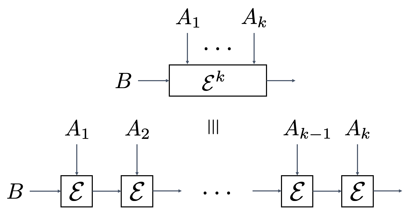
Figure 3: Representation of a $C^{*}$-finitely correlated state.

We use the symbol $\mathcal{E}$ instead of $\mathbb{E}$ when dealing with realizations to distinguish them among realizations. Note, that whenever we find a realization with memory system being a $C^{*}$-algebra and generating map $\mathbb{E}$ being completely positive in the natural $C^{*}$ order, we can always find a realization satisfying the same that is of the form described in Definition 2.8, even with $\rho_{0}$ being of full support, see [8, Lem. 2.5].

As before we will also use the notation $\mathcal{E}_{A}(B)=\mathcal{E}(A\otimes B)$.

We can apply the construction of the quotient realization Proposition 2.4, that is we set

$$\mathcal{W}=\{\mathcal{E}^{t^{*}}_{A}(\mathds{1}_{\mathcal{B}})\ |\ A\in\mathcal{C}_{R}\}\,,\qquad\text{ and }\qquad\tilde{\mathcal{W}}=\{\rho_{0}\mathcal{E}^{t^{*}}_{A}\ |\ A\in\mathcal{C}_{L}\}$$ (34)

where we recall the notation $\mathcal{E}^{k}(A_{1}\otimes\dots\otimes A_{k}\otimes B)=\mathcal{E}_{A_{1}}\mathcal{E}_{A_{2}}\cdots\mathcal{E}_{A_{k}}(B)$ (see Figure 3). We also set

$$\mathcal{V}:=\mathcal{W}/({\mathcal{W}\cap\tilde{\mathcal{W}}^{\perp}})\subseteq\mathcal{W}$$ (35)

and define the projection $L:\mathcal{W}\rightarrow\mathcal{V}$.

Other than in the general case, the Hilbert Schmidt inner product lets us identify the quotient $\mathcal{V}$ with the orthogonal complement $\mathcal{V}^{\prime}$ of $\mathcal{W}\cap\tilde{\mathcal{W}}^{\perp}$ in $\mathcal{W}$ and denote the unique map doing so as $R:\mathcal{\mathcal{V}\rightarrow\mathcal{V}^{\prime}}$. It satisfies $RL=\Pi_{\mathcal{V}^{\prime}}$ where $\Pi_{\mathcal{V}^{\prime}}$ is the orthogonal projector onto $\mathcal{V}^{\prime}$.

Lemma 2.6 then takes the following form:

Lemma 2.9.

$U^{\intercal}\mathcal{F}$ is invertible on $\mathcal{V}^{\prime}$ with inverse $(U^{\intercal}\mathcal{F}|_{\mathcal{V}^{\prime}})^{-1}=RM^{-1}$

2.2.3 Empirical realizations

It will be useful to also consider the following realizations, obtained by a similarity transformation of the observable realization. In the following $\hat{U}$ can be thought as a truncated left orthogonal map in the SVD of $\hat{\Omega}$, which is an estimate of $\Omega$ (cf.  Section 4). While the realization constructed from $\hat{\Omega}$ will not be an exact realization of $\omega$, the empirical realization constructed here is, and will be easier to compare with the estimate than the observable realization.

Proposition 2.10 (Empirical realizations).

Let $\omega$ be a translation invariant state with observable realization $(\mathbb{C}^{m},e,\mathbb{K},\rho)$. For any map $\hat{U}:\mathbb{C}^{m}\rightarrow\mathcal{C}_{L}^{*}$ (real in the basis of self-adjoint elements) such that $\hat{U}^{\intercal}U$ is invertible, the quadruple $(\mathbb{C}^{m},\tilde{e},\tilde{\mathbb{K}},\tilde{\rho})$ given by

$$\tilde{e} ={\hat{U}}^{\intercal}\Omega(\mathds{1}),$$ (36)

$$\tilde{\rho} =\tau\Omega(\hat{U}^{\intercal}\Omega)^{+},$$ (37)

$$\tilde{\mathbb{K}}_{A} ={\hat{U}}^{\intercal}(\Omega_{A})({\hat{U}}^{\intercal}\Omega)^{+}\,.$$ (38)

is a realization of $\omega$, in fact

$$\tilde{e} =\hat{U}^{\intercal}Ue,$$ (39)

$$\tilde{\rho} =\rho(\hat{U}^{\intercal}U)^{-1},$$ (40)

$$\tilde{\mathbb{K}}_{A} =\hat{U}^{\intercal}U\mathbb{K}_{A}(\hat{U}^{\intercal}U)^{-1}.$$ (41)

Any such realization is called empirical realization.

The following proposition links empirical realizations with quotient realizations, and in particular with quotient realizations of completely positive ones. Let us define the map

$$\hat{M}:=\hat{U}^{\intercal}UM\,,$$ (42)

where $M$ is the linear map connecting a quotient realization with the observable realization, as in Proposition 2.7. The following proposition easily follows.

Proposition 2.11 (Empirical realizations and quotient realization).

For an empirical realization as in Proposition 2.10, and a quotient realization as in Proposition 2.7, we have

$$\tilde{e} =\hat{M}e^{\prime},$$ (43)

$$\tilde{\mathbb{K}}_{A} =\hat{U}^{\intercal}U\mathbb{K}_{A}(\hat{U}^{\intercal}U)^{-1}=\hat{M}\mathbb{K}^{\prime}_{A}\hat{M}^{-1},$$ (44)

$$\tilde{\rho} =\rho^{\prime}\hat{M}^{-1}.$$ (45)

so that

$$\tilde{e} =\hat{M}Lu,$$ (46)

$$\tilde{\mathbb{K}}_{A}\hat{M}L =M\mathbb{K}^{\prime}_{A}L=ML\mathbb{E}_{A}|_{W},$$ (47)

$$\tilde{\rho}\hat{M}L =\sigma|_{W},$$ (48)

and, hence,

$$\tilde{\mathbb{K}}^{t}_{X_{1}\otimes\cdots\otimes X_{t}}\tilde{e}=\tilde{\mathbb{K}}_{X_{1}}\cdots\tilde{\mathbb{K}}_{X_{t}}\hat{M}Lu=\hat{M}L\mathbb{E}^{t}_{X_{1}\otimes\cdots\otimes X_{t}}u\,.$$ (49)

3 Operator systems and realizations

The memory system of a finitely correlated state $\omega$ is by definition a finite-dimensional operator system (cf. Appendix A), which means that it can be represented as a finite-dimensional subspace of some algebra $\mathcal{B}(\mathcal{H})$. However, the underlying Hilbert space $\mathcal{H}$ does not need to be finite-dimensional, and indeed there are examples of operator systems that can only be embedded into infinite-dimensional $C^{*}$-algebras (see [30, Thm. 2.4] together with the fact that the group $C^{*}$-algebra of a free group is infinite-dimensional). Moreover, an arbitrary finitely correlated state is not necessarily $C^{*}$-finitely correlated (in fact, already in the abelian case [11] there are counterexamples, but we don’t know of properly non-commutative examples). Now, it is true that $C^{*}$-finitely correlated states are weak-$*$-dense in all translation invariant states [8, Prop. 2.6]. Thus, we cannot distinguish between $C^{*}$-finitely correlated states and a generic translation invariant state by measuring only finitely many observables up to precision $\varepsilon>0$. But since the memory size needed to realize these approximating $C^{*}$-finitely correlated states will usually diverge with the size of the region where the observables are supported, we are also interested in extending the algorithm directly to the case of a general finitely correlated state.

The order we consider in the following is constructed by taking $\Psi_{n}(X)$ to be positive if $X$ is positive. This construction can als be dualized which gives us a minimal and a maximal order. This will implicitly be used in the proof of Lemma 3.1 and is commented on in Remark 3.3. The order gives rise to an order norm $\|\Psi_{X}\|_{\Psi_{\mathds{1}}}$ (see Appendix A) that in the case of a $C^{*}$ order yields back the $C^{*}$ norm. In addition to this generalized operator norm, we will also need an analogue of the the Hilbert-Schmidt norm for the estimates in Section 4.3. Since we cannot guarantee the memory systems to be represented on a finite-dimensional Hilbert space we cannot directly use the Hilbert-Schmidt norm. However, we can use the maps $\Psi_{X}$ defined in Equation (13) to define an inner product. For $X\in\mathcal{A}_{[1,t^{*}]}$ set $\xi_{X}(i)=\operatorname{Tr}\left(XX_{i}\right)$ and $X^{\prime}=\sum_{i}\Psi_{X}(X_{i})X_{i}$. Then clearly $\Psi_{X}(Y)=\operatorname{Tr}\left(X^{\prime}Y\right)$ and $\xi_{X^{\prime}}(i)=\Psi_{X}(X_{i})$, so $\xi_{X^{\prime}}=\ddot{\Omega}\xi_{X}$ where $\ddot{\Omega}_{ij}=\omega(X_{i}\otimes X_{j})$ (‘Ömega’) is $\Omega$ written in coordinates. Furthermore, $\Psi_{X}=\Psi_{Z}$ if and only if $\xi_{X^{\prime}}=\xi_{Z^{\prime}}$ if and only if $X^{\prime}=Z^{\prime}$. We then set

$$(\Psi_{X},\Psi_{Y})_{\Omega}:=\operatorname{Tr}\left((X^{\prime})^{*}Y^{\prime}\right)=\xi_{X^{\prime}}\cdot\xi_{Y^{\prime}}=\sum_{i}\overline{\Psi_{X}(X_{i})}\Psi_{Y}(X_{i})$$

where $x\cdot y=\sum_{I}\overline{x(I)}y(I)$ is the inner product on $\mathbb{C}^{d^{t^{*}}}$. $(\cdot,\cdot)_{\Omega}$ thus defines an inner product on $V$. We denote the corresponding norm by $\|\cdot\|_{\Omega}$ and observe the following inequalities:

Lemma 3.1.

Let $X\in\mathcal{A}_{[1,t^{*}]}=\mathcal{C}_{R}$. It holds that $\|{\Psi_{X}}\|_{\Psi_{\mathds{1}}}\leq\|P(X)\|_{2}$, where $P$ is the Hilbert-Schmidt orthogonal projection onto $\operatorname{supp}(\Omega)$, and

$$\sigma_{m}(\Omega)\|{\Psi_{X}}\|_{\Psi_{\mathds{1}}}\leq\|\Psi_{X}\|_{\Omega}\leq\|\Psi_{X}\|_{\Psi_{\mathds{1}}}.$$ (50)

Proof.

First, we observe that $\Psi_{P(X)}=\Psi_{X}$ by definition of $P$, and that $\Psi$ is completely positive and unital, thus contractive. Then

$$\|\Psi_{X}\|_{\Psi_{\mathds{1}}}=\|\Psi_{P(X)}\|_{\Psi_{\mathds{1}}} \leq\|P(X)\|_{\infty}\leq\|P(X)\|_{2}\,.$$

Next, we have

$$\|{\Psi_{X}}\|_{\Omega}^{2}=\|{\Psi_{P(X)}}\|_{\Omega}^{2}=(\ddot{\Omega}\xi_{P(X)})\cdot(\ddot{\Omega}\xi_{P(X)})\geq\sigma_{m}(\Omega)^{2}\xi_{P(X)}\cdot\xi_{P(X)}=\sigma_{m}(\Omega)^{2}\|{P(X)}\|^{2}_{2}\,.$$

For the last inequality, consider the matrix amplification $\Psi_{2}$ of $\Psi$ on $\mathbb{M}_{2}(\mathcal{C}_{R})$ mapping to $\mathbb{M}_{2}(\mathcal{C}_{L}^{*})\cong\mathbb{M}_{2}(\mathcal{C}_{L})^{*}$ (the isomorphism is implemented by letting $A\otimes\varphi$ act on $B\otimes X$ as $(A\otimes\varphi).(B\otimes X):=\operatorname{Tr}\left(AB\right)\varphi(X)$). In particular, $\Psi_{2}$ is completely positive. For $X\in\mathcal{C}_{R}$ let

$$S(X)=\begin{pmatrix}0&X\\ X^{*}&0\end{pmatrix}=|0\rangle\!\langle 1|\otimes X+|1\rangle\!\langle 0|\otimes X^{*}$$

be the embedding of $\mathcal{C}_{R}$ as self-adjoint elements in $\mathbb{M}_{2}(\mathcal{C}_{R})$. Note that $\Psi_{2,S(X)}=S(\Psi_{X})$. Let $\lambda\geq\|X^{\prime}\|_{\infty}$ so that $\lambda\mathds{1}-S(X^{\prime})$ is a positive matrix. Furthermore, let $r>0$. We then have that

$$\Psi_{2,r\mathds{1}+S(X)}(\lambda\mathds{1}-S(X^{\prime}))= r\lambda(\mathrm{id}_{\mathbb{M}_{2}}\otimes\Psi_{\mathds{1}}).\mathds{1}+\lambda S(\Psi_{X}).\mathds{1}$$

$$-r(\mathrm{id}_{\mathbb{M}_{2}}\otimes\Psi_{\mathds{1}}).S(X^{\prime})-S(\Psi_{X}).S(X^{\prime})$$

$$= 2r\lambda-S(\Psi_{X}).S(X^{\prime}).$$

Here, we used $(\mathrm{id}_{\mathbb{M}_{2}}\otimes\Psi_{\mathds{1}}).\mathds{1}=2$ and that if $A$ is block-diagonal and $B$ is ‘block-off-diagonal’ then $(A\otimes\varphi).(B\otimes X)=0$. Now, we have that

$$S(\Psi_{X}).S(X^{\prime})=\Psi_{X}((X^{\prime})^{*})+\Psi_{X^{*}}(X^{\prime})=2\|{\Psi_{X}}\|_{\Omega}^{2}.$$

We find that

$$\Psi_{2,r\mathds{1}+S(X)}(\lambda\mathds{1}-S(X^{\prime}))=2(r\lambda-\|\Psi_{X}\|_{\Omega}^{2})\,.$$

Thus, choosing $\lambda=\|\Psi_{X}\|_{\Omega}=\|X^{\prime}\|_{2}\geq\|{X^{\prime}}\|_{\infty}$ and $r<\|\Psi_{X}\|_{\Omega}$ we find

$$r\|\Psi_{X}\|_{\Omega}<\|\Psi_{X}\|_{\Omega}^{2}$$

showing that $\Psi_{2,r\mathds{1}+S(X)}$ is not a positive functional. By definition of the order norm this shows $r\leq\|\Psi_{X}\|_{\Psi_{\mathds{1}}}$ and thus the desired norm inequality (cf. also Remark 3.3). ∎

Remark 3.2.

Replacing $\mathcal{C}_{R}$ by $\mathbb{M}_{n}(\mathcal{C}_{R})\cong\mathbb{M}_{n}\otimes\mathcal{C}_{R}$ (similarly for $\mathcal{C}_{L}$) and $\Psi$ by its $n$-th amplification $\Psi_{n}$, we can apply the above proof mutatis mutandis. This yields the inequality

$$\|\cdot\|_{n,\Omega}\leq\sqrt{n}\|\cdot\|_{{\Psi_{n}}(\mathds{1})}$$

for the norm on $\mathbb{M}_{n}(\mathcal{C}_{R})$.

The inequalities in Lemma 3.1 hold for the norms defined on the memory system of the abstract (minimal) realization. Consider the restriction of $U^{\intercal}$ to $V$, $\Psi_{X}\mapsto U^{\intercal}\Psi_{X}$, which is invertible. It induces an operator system structure on $\mathbb{C}^{m}$ that is completely order isomorphic to the order structure of the regular realization and it holds that $U^{\intercal}\Psi_{\mathds{1}}=e$ as defined in Section 2.2.1. Also note that $\lVert(\mathrm{id}_{\mathbb{M}_{n}}\otimes U^{\intercal})\Psi_{n,X}\rVert_{2}=\lVert\Psi_{X}\rVert_{n,\Omega}$.

In particular, the following inequalities hold for $x\in\mathbb{M}_{n}(\mathbb{C}^{m})$:

$$\sigma_{m}(\Omega)\lVert x\rVert_{\mathds{1}_{\mathbb{M}_{n}}\otimes e}\leq\lVert x\rVert_{2}\leq\sqrt{n}\lVert x\rVert_{\mathds{1}_{\mathbb{M}_{n}}\otimes e}$$ (51)

where $\lVert\cdot\rVert_{2}$ is just the standard euclidean norm.

Remark 3.3.

In fact, the matrix order on the memory system $V$ is not unique. The construction in [8] mentioned in the beginning of this section can be applied to both sides of the chain. Dualizing the order on one side then gives a matrix order on the other side and the two need not coincide. However, every positive element in the directly constructed one is also positive in the one obtained through dualizing and in fact every admissible matrix order making the generating map $\mathbb{E}$ completely positive has to lie between the two orders. We may thus call them minimal and maximal and since the cones of the minimal matrix order are smaller than those of the maximal matrix order, the corresponding order norms satisfy the reverse inequality. This has also been observed by I. Todorov [31] (and possibly others). The proof of Lemma 3.1 works for the minimal matrix order for the leftmost inequality and implicitly uses the maximal matrix order for the rightmost. Therefore, the bounds are valid for the order norm of any admissible matrix order.

Remark 3.4.

Every bipartite state between two $C^{*}$-algebras gives rise to operator system structures analogous to Remark 3.3. Assuming that this operator system is finite-dimensional, it is also sufficient to consider a finite-dimensional subspace of the algebra, which can be assumed to be an operator (sub) system. If this operator subsytem can be represented on a finite-dimensional Hilbert space, we can again use the Hilbert-Schmidt inner product to define a norm on the space of ‘correlation functionals’ that satisfies the bounds as in Lemma 3.1. This might be useful to obtain bounds in other settings. We are not aware of this being mentioned in the literature explicitly in this context. However, the results of [32, 31, 33] are very close to this.

Remark 3.5.

We also note that a quotient realization of a $C^{*}$-finitely correlated state can be given the structure of an abstract operator system, which is not necessarily the minimal or the maximal order, but is inherited by the usual matrix order on $\mathcal{B}$. $\mathcal{V}=\mathcal{W}/{\mathcal{W}\cap\tilde{\mathcal{W}}^{\perp}}$ can also be given the structure of an operator system, with unit $e^{\prime}=L\mathds{1}_{\mathcal{B}}$ and cones $C_{n}:=L(\mathbb{M}_{n}(\mathcal{W})^{+})$.

By “push-forward” via the invertible map $M$, the observable realization also gets an operator system structure and $M$ automatically becomes unital and completely positive. The map $R$ identifying $\mathcal{V}$ with $\mathcal{V}^{\prime}\subset\mathcal{W}$, see Lemma 2.9, then is a (unital) complete order isomorphism. $\mathcal{V}$ then inherits the Hilbert-Schmidt norm from $\mathcal{B}$, which we denote as $\lVert\cdot\rVert_{2}$ without ambiguity. Then, for $x\in\mathbb{M}_{n}(\mathcal{V})$ we have $\lVert x\rVert_{(Le^{\prime})^{(n)}}\leq\lVert Rx\rVert_{\mathds{1}_{\mathbb{M}_{n}(\mathcal{B})}}\leq\lVert x\rVert_{2}$ by contractivity of $L$ and the standard inequality between Schatten norms.

We thus have

$$\lVert\mathrm{id}_{\mathbb{M}_{n}}\otimes U^{\intercal}\mathcal{F}R\rVert_{\mathds{1}_{\mathbb{M}_{n}}\otimes Le^{\prime}\rightarrow 2}\leq\lVert\mathrm{id}_{\mathbb{M}_{n}}\otimes\mathrm{id}_{\mathbb{C}^{m}}\rVert_{e\rightarrow 2}\lVert\mathrm{id}_{\mathbb{M}_{n}}\otimes U^{\intercal}\mathcal{F}R\rVert_{\mathds{1}_{\mathbb{M}_{n}}\otimes Le^{\prime}\rightarrow{\mathds{1}_{\mathbb{M}_{n}}\otimes e}}\leq\sqrt{n}.$$ (52)

4 State reconstruction for FCS

Given a finitely-correlated state $\omega$ on the infinite chain, we denote its restriction to $\mathcal{A}_{[1,t]}$ as $\omega_{t}$, i.e.

$$\omega_{t}(X_{1}\otimes\cdots\otimes X_{t}):=\rho\mathbb{K}_{X_{1}}\cdots\mathbb{K}_{X_{t}}e\,.$$ (53)

Consider the corresponding map $\Omega_{(\cdot)}:(A,A^{\prime})\mapsto\Omega_{A}(A^{\prime})$ as defined in Equation (16) and its observable realization $(\mathbb{C}^{m},e,\mathbb{K},\rho)$ as in Proposition 2.5. We can reconstruct an approximation of the realization parameters from an estimate $\hat{\Omega}_{(\cdot)}$ obtained from estimating the expectation values of $\omega_{t}$. Here, we need to impose that the estimate $\hat{\Omega}$ has at least rank $m$, and we take its $m$-truncated singular value decomposition, meaning that we only retain the first $m$ singular values and singular vectors. This means that $\hat{U}$ is the matrix of the first $m$ left singular vectors of $\hat{\Omega}$.

Definition 4.1 (Spectral state reconstruction).

$$\hat{\omega}_{t}(X_{1}\otimes\cdots\otimes X_{t}):=\hat{\rho}\hat{\mathbb{K}}_{X_{1}}\cdots\hat{\mathbb{K}}_{X_{t}}\hat{e},$$ (54)

where

$$\hat{e} ={\hat{U}}^{\intercal}\hat{\Omega}(\mathds{1}),$$ (55)

$$\hat{\rho} =\tau\hat{U}=\tau\hat{\Omega}(\hat{U}^{\intercal}\hat{\Omega})^{+},$$ (56)

$$\hat{\mathbb{K}}_{A} ={\hat{U}}^{\intercal}(\hat{\Omega}_{A})({\hat{U}}^{\intercal}\hat{\Omega})^{+}\,.$$ (57)

To bound the accuracy of the estimate $\hat{\omega}_{t}$ it is convenient to compare the above empirical reconstruction with the empirical realization, rather than the observable realization.

4.1 Empirical estimates of realization parameters

In the following, we obtain bounds on the estimates of realization parameters, in terms of the accuracy of the estimation of the marginals.

Lemma 4.2.

If $\|\Omega-\hat{\Omega}\|_{2\rightarrow 2}\leq\frac{\sigma_{m}(\Omega)}{3}$, it holds that:

$$\|\tilde{\mathbb{K}}-\hat{\mathbb{K}}\|_{2\rightarrow 2} \leq\frac{1+\sqrt{5}}{2}\frac{\|\Omega-\hat{\Omega}\|_{2\rightarrow 2}}{\min\{\sigma_{m}(\hat{\Omega}),\sigma_{m}(\hat{U}^{\intercal}\Omega)\}^{2}}+\frac{\|\Omega_{(\cdot)}-\hat{\Omega}_{(\cdot)}\|_{2\rightarrow 2}}{\sigma_{m}(\hat{U}^{\intercal}\hat{\Omega})},$$ (58)

$$\leq 4\left(\frac{\|\Omega-\hat{\Omega}\|_{2}}{\sigma_{m}({\Omega})^{2}}+\frac{\|\Omega_{(\cdot)}-\hat{\Omega}_{(\cdot)}\|_{2}}{3\sigma_{m}(\Omega)}\right),$$ (59)

$$\|\hat{e}-\tilde{e}\|_{2} \leq\|\big{(}\Omega-\hat{\Omega}\big{)}(\mathds{1})\|_{2},$$ (60)

$$\|\hat{\rho}-\tilde{\rho}\|_{2} \leq\frac{1+\sqrt{5}}{2}\frac{\|\hat{\Omega}-\Omega\|_{2}}{\min\{\sigma_{m}(\hat{\Omega}),\sigma_{m}(\hat{U}^{\intercal}\Omega)\}^{2}}+\frac{\|\tau\big{(}\hat{\Omega}-\Omega\big{)}\|_{2}}{\sigma_{m}(\hat{U}^{\intercal}\hat{\Omega})}\,$$ (61)

$$\leq 4\left(\frac{\|\hat{\Omega}-\Omega\|_{2}}{\sigma_{m}(\Omega)^{2}}+\frac{\|\tau\big{(}\hat{\Omega}-\Omega\big{)}\|_{2}}{3\sigma_{m}(\Omega)}\right).$$ (62)

$$\|(\hat{U}^{\intercal}U)^{-1}\|_{2\rightarrow 2} \leq\frac{2}{\sqrt{3}}$$ (63)

Proof.

In order to bound

$$\|\tilde{\mathbb{K}}-\hat{\mathbb{K}}\|_{2\rightarrow 2}=\sup_{X\in\mathcal{A}\otimes\mathbb{C}^{m},\,\|X\|_{2}\leq 1}\|(\tilde{\mathbb{K}}-\hat{\mathbb{K}})(X)\|_{2},$$ (64)

note that, by Equations (38) and (57),

$$\|\tilde{\mathbb{K}}-\hat{\mathbb{K}}\|_{2\rightarrow 2}=\|\hat{U}^{\intercal}(\Omega_{(\cdot)})(\hat{U}^{\intercal}\Omega)^{+}-\hat{U}^{\intercal}(\hat{\Omega}_{(\cdot)})(\hat{U}^{\intercal}\hat{\Omega})^{+}\|_{2\rightarrow 2}$$ (65)

By triangular inequalities,

$$\|\tilde{\mathbb{K}}-\hat{\mathbb{K}}\|_{2\rightarrow 2} \leq\|\hat{U}^{\intercal}(\Omega_{(\cdot)})\left((\hat{U}^{\intercal}\Omega)^{+}-(\hat{U}^{\intercal}\hat{\Omega})^{+}\right)\|_{2\rightarrow 2}+\|\hat{U}^{\intercal}(\Omega_{(\cdot)}-\hat{\Omega}_{(\cdot)})(\hat{U}^{\intercal}\hat{\Omega})^{+}\|_{2\rightarrow 2}\,.$$ (66)

Therefore using Lemma B.2 and the inequality $\|A\|_{2\rightarrow 2}=\lVert A\rVert_{\infty}\leq\|A\|_{2}$ and the fact that $\sigma_{m}(\hat{\Omega})=\sigma_{m}(\hat{U}^{\intercal}\hat{\Omega})$,

$$\|\tilde{\mathbb{K}}-\hat{\mathbb{K}}\|_{2\rightarrow 2} \leq\|\Omega_{(\cdot)}\|_{2}\frac{1+\sqrt{5}}{2}\frac{\|\Omega-\hat{\Omega}\|_{2\rightarrow 2}}{\min\{\sigma_{m}(\hat{\Omega}),\sigma_{m}(\hat{U}^{\intercal}\Omega)\}^{2}}+\frac{\|\Omega_{(\cdot)}-\hat{\Omega}_{(\cdot)}\|_{2\rightarrow 2}}{\sigma_{m}(\hat{U}^{\intercal}\hat{\Omega})}.$$ (67)

Moreover, given bases $\{X_{\ell}\}_{\ell=1}^{m_{1}}$, $\{A_{j}\}_{j=1}^{d^{2}}$, $\{Y_{i}\}_{i=1}^{m_{2}}$ of $\mathcal{C}_{R}$, $\mathcal{A}$ and $\mathcal{C}_{L}$, respectively,

$$\|\Omega_{(\cdot)}\|_{2} \leq\sqrt{\sum_{i=1}^{m_{2}}\sum_{j=1}^{d^{2}}\sum_{l=1}^{m_{1}}|\omega(Y_{i}\otimes A_{j}\otimes X_{\ell})|^{2}}\leq\sqrt{\operatorname{Tr}[\omega_{2t^{*}+1}^{2}]}\leq 1\,.$$ (68)

Therefore,

$$\|\tilde{\mathbb{K}}-\hat{\mathbb{K}}\|_{2\rightarrow 2} \leq\frac{1+\sqrt{5}}{2}\frac{\|\Omega-\hat{\Omega}\|_{2\rightarrow 2}}{\min\{\sigma_{m}(\hat{\Omega}),\sigma_{m}(\hat{U}^{\intercal}\Omega)\}^{2}}+\frac{\|\Omega_{(\cdot)}-\hat{\Omega}_{(\cdot)}\|_{2\rightarrow 2}}{\sigma_{m}(\hat{U}^{\intercal}\hat{\Omega})}.$$ (69)

For the second inequality, using the expressions for $\tilde{e}$ and $\hat{e}$ given in Equations (36) and (55) respectively

$$\|\hat{e}-\tilde{e}\|_{2} =\|\hat{U}^{\intercal}\big{(}\Omega-\hat{\Omega}\big{)}(\mathds{1})\|_{2}$$ (70)

$$\leq\|\hat{U}^{\intercal}\|_{2\rightarrow 2}\|\big{(}\Omega-\hat{\Omega}\big{)}(\mathds{1})\|_{2}$$ (71)

$$\leq\|\big{(}\Omega-\hat{\Omega}\big{)}(\mathds{1})\|_{2}$$ (72)

For the third inequality, using the expressions for $\tilde{\rho}$ and $\hat{\rho}$ given in Equations (37) and (56) respectively,

$$\|\hat{\rho}-\tilde{\rho}\|_{2} =\|\tau\big{(}\hat{\Omega}(\hat{U}^{\intercal}\hat{\Omega})^{+}-\Omega(\hat{U}^{\intercal}\Omega)^{+}\big{)}\|_{2}$$ (73)

$$\leq\|\tau\big{(}{\Omega}(\hat{U}^{\intercal}\hat{\Omega})^{+}-\Omega(\hat{U}^{\intercal}\Omega)^{+}\big{)}\|_{2}+\|\tau\big{(}\hat{\Omega}(\hat{U}^{\intercal}\hat{\Omega})^{+}-\Omega(\hat{U}^{\intercal}\hat{\Omega})^{+}\big{)}\|_{2}$$ (74)

$$\leq\|(\hat{U}^{\intercal}\hat{\Omega})^{+}-(\hat{U}^{\intercal}\Omega)^{+}\|_{2\rightarrow 2}\|\tau\Omega\|_{2}+\|(\hat{U}^{\intercal}\hat{\Omega})^{+}\|_{2\rightarrow 2}\|\tau\big{(}\hat{\Omega}-\Omega\big{)}\|_{2}\,.$$ (75)

Then using $\|\tau\Omega\|_{2}=\sqrt{\sum_{i=1}^{m_{1}}{\omega}(X_{i})^{2}}\leq 1$ and Lemma B.2,

$$\|\hat{\rho}-\tilde{\rho}\|_{2} \leq\frac{1+\sqrt{5}}{2}\frac{\|\hat{\Omega}-\Omega\|_{2}}{\min\{\sigma_{m}(\hat{\Omega}),\sigma_{m}(\hat{U}^{\intercal}\Omega)\}^{2}}+\frac{\|\tau\big{(}\hat{\Omega}-\Omega\big{)}\|_{2}}{\sigma_{m}(\hat{U}^{\intercal}\hat{\Omega})}\,.$$ (76)

Then,  (59), (62), (63) directly follow from perturbation bounds for singular values, which are collected in Appendix B, and in particular Lemma B.5. For these bounds we closely follow the treatment of previous works in the classical setting [12, 18, 19]. ∎

4.2 Error propagation bound

With $(\mathbb{C}^{m},\mathcal{K},e,\rho)$ being the observable realization Proposition 2.5, in the following we will assume that $\mathcal{V}$ is an operator system with order unit $e^{\prime}$ and $M:\mathcal{V}\rightarrow\mathbb{C}^{m}$ is an invertible linear map such that $Me^{\prime}=e$ and that $\rho^{\prime}=\rho M$ is a positive functional. It holds that $\rho^{\prime}(e^{\prime})=1$ and that the map ${M}^{-1}{\mathbb{K}}{M}$ is unital, in the sense that ${M}^{-1}{\mathbb{K}}_{\mathds{1}_{\mathcal{A}}}{M}e^{\prime}=e^{\prime}$. We further assume that it is completely positive. Of course, we can always take $\mathcal{V}$ to be the vector space of functionals $\Psi_{A}$, $A\in\mathcal{A}_{R}$, whose positive elements at level $n$ are $\Psi_{n}(A)$, $A\in\mathbb{M}_{n}(A)^{+}$. The following error parameters will be used in the analysis: given $\widetilde{e}$, $\widetilde{\rho}$, $\widetilde{\mathbb{K}}_{A}$ and $\hat{M}$ as in Equations (39), (40), (41) and (42). respectively, where $\hat{U}$ and is chosen as in Definition 4.1,

$$\delta_{1} :=\|(\hat{\rho}-\tilde{\rho})\hat{M}\|_{e^{\prime},*},$$ (77)

$$\delta_{\infty} :=\|\hat{M}^{-1}(\tilde{e}-\hat{e})\|_{e^{\prime}},$$ (78)

$$\Delta :=\|\hat{M}^{-1}(\tilde{\mathbb{K}}-\hat{\mathbb{K}})\hat{M}\|_{\mathds{1}\otimes e^{\prime}\rightarrow e^{\prime},cb}.$$ (79)

Above, we denote by $\tilde{\mathbb{K}}:\mathcal{A}\otimes\mathbb{C}^{m}\to\mathbb{C}^{m}$ and $\hat{\mathbb{K}}:\mathcal{A}\otimes\mathbb{C}^{m}\to\mathbb{C}^{m}$ the maps $A\otimes x\mapsto\tilde{\mathbb{K}}_{A}(x)$ and $A\otimes x\mapsto\hat{\mathbb{K}}_{A}(x)$, respectively.

Our first main result is the following error propagation bound. We write $\|\cdot\|_{1}$ since finite-size marginals are essentially density operators. Furthermore, if $\|\cdot\|$ is any norm, we denote the corresponding norm on the dual space by $\|\cdot\|_{*}$, so $\|\cdot\|_{1}\equiv\|\cdot\|_{\mathscr{A},*}$ if $\mathscr{A}$ denotes an arbitrary $C^{*}$-algebra. We recall that for maps between two spaces with norms $\|\cdot\|_{a}$ and $\|\cdot\|_{b}$, say, we denote the corresponding operator norm as $\|\cdot\|_{a\to b}$, so, e.g., $\|\cdot\|_{a,*}=\|\cdot\|_{a\rightarrow p}$ for any $p$-norm on $\mathbb{C}$.

Theorem 4.3 (Error propagation).

Let $\omega$ be a finitely correlated state. For the state reconstruction in Definition 4.1, and the error parameters defined in Eqs. (77), (78) and (79), if $\hat{U}^{\intercal}U$ is invertible, then

$$\|\hat{\omega}_{t}-\omega_{t}\|_{1}\leq(1+\delta_{1})(1+\delta_{\infty})(1+\Delta)^{t}-1.$$ (80)

Proof of Theorem 4.3.

By the triangle inequality, we have the following bound

$$\|\hat{\omega}_{t}-\omega_{t}\|_{1} \leq\underbrace{\|(\hat{\rho}-\tilde{\rho})\tilde{\mathbb{K}}^{t}\tilde{e}\|_{1}}_{(\operatorname{I})}+\underbrace{\|(\hat{\rho}-\tilde{\rho})(\hat{\mathbb{K}}^{t}\hat{e}-\tilde{\mathbb{K}}^{t}\tilde{e})\|_{1}}_{(\operatorname{II})}+\underbrace{\|\tilde{\rho}(\tilde{\mathbb{K}}^{t}\tilde{e}-\hat{\mathbb{K}}^{t}\hat{e})\|_{1}}_{(\operatorname{III})}$$ (81)

Let us start with $(\operatorname{I})$. By Equations (39) and (41),

$$\|(\hat{\rho}-\tilde{\rho})\tilde{\mathbb{K}}^{t}\tilde{e}\|_{1} =\|(\hat{\rho}-\tilde{\rho})\hat{M}M^{-1}\mathbb{K}^{t}M(e^{\prime})\|_{1}$$

$$\leq\lVert(\hat{\rho}-\tilde{\rho})\hat{M}\rVert_{e^{\prime},*}\lVert M^{-1}\mathbb{K}^{t}M(e^{\prime})\rVert_{\infty\rightarrow e^{\prime}}$$ (82)

$$=\lVert(\hat{\rho}-\tilde{\rho})\hat{M}\rVert_{e^{\prime},*}\,,$$ (83)

where we used that $\lVert M^{-1}\mathbb{K}^{t}M(e^{\prime})\rVert_{\infty\rightarrow e^{\prime}}=1$ because $M^{-1}\mathbb{K}^{t}M$ is unital. By similar arguments, $(\operatorname{II})$ is bounded as

$$\|(\hat{\rho}-\tilde{\rho})(\tilde{\mathbb{K}}^{t}\tilde{e}-\hat{\mathbb{K}}^{t}\hat{e})\|_{1} \leq\lVert(\hat{\rho}-\tilde{\rho})\hat{M}\rVert_{e^{\prime},*}\|(\hat{M})^{-1}(\tilde{\mathbb{K}}^{t}\tilde{e}-\hat{\mathbb{K}}^{t}\hat{e})\|_{\infty\rightarrow e^{\prime}},$$ (84)

using invertibility of $\hat{U}^{\intercal}U$. Finally, we bound $(\operatorname{III})$:

$$\|\tilde{\rho}(\tilde{\mathbb{K}}^{t}\tilde{e}-\hat{\mathbb{K}}^{t}\hat{e})\|_{1} \leq\|\tilde{\rho}\hat{M}\|_{e^{\prime},*}\|\hat{M}^{-1}(\tilde{\mathbb{K}}^{t}\tilde{e}-\hat{\mathbb{K}}^{t}\hat{e})\|_{\infty\rightarrow e^{\prime}}$$

$$\leq\|\rho M\|_{e^{\prime},*}\|\hat{M}^{-1}(\tilde{\mathbb{K}}^{t}\tilde{e}-\hat{\mathbb{K}}^{t}\hat{e})\|_{\infty\rightarrow e^{\prime}}$$ (85)

$$=\|\hat{M}^{-1}(\tilde{\mathbb{K}}^{t}\tilde{e}-\hat{\mathbb{K}}^{t}\hat{e})\|_{\infty\rightarrow e^{\prime}},$$ (86)

where we also used that $\rho^{\prime}=\rho M$ is a non-negative functional and $\rho^{\prime}(e^{\prime})=1$. By definition of the cb norm, the triangle inequality, and denoting $\hat{e}_{t}:=\hat{\mathbb{K}}^{t}\hat{e}$ and $\tilde{e}_{t}:=\tilde{\mathbb{K}}^{t}\tilde{e}$,

$$\|\hat{M}^{-1}(\tilde{\mathbb{K}}^{t}\tilde{e}-\hat{\mathbb{K}}^{t}\hat{e})\|_{\infty\to e^{\prime}} \leq\|\hat{M}^{-1}(\tilde{\mathbb{K}}^{t}\tilde{e}-\hat{\mathbb{K}}^{t}\hat{e})\|_{\infty\rightarrow e^{\prime},cb}$$ (87)

$$\leq\underbrace{\|\hat{M}^{-1}(\tilde{\mathbb{K}}-\hat{\mathbb{K}})\tilde{e}_{t-1}\|_{\infty\rightarrow e^{\prime},cb}}_{(\operatorname{I}^{\prime})}$$ (88)

$$+\underbrace{\|\hat{M}^{-1}(\tilde{\mathbb{K}}-\hat{\mathbb{K}})(\hat{e}_{t-1}-\tilde{e}_{t-1})\|_{\infty\rightarrow e^{\prime},cb}}_{(\operatorname{II}^{\prime})}$$

$$+\underbrace{\|\hat{M}^{-1}\tilde{\mathbb{K}}^{t}(\tilde{e}_{t-1}-\hat{e}_{t-1})\|_{\infty\rightarrow e^{\prime},cb}}_{(\operatorname{III}^{\prime})}\,.$$ (89)

For the first piece $(\operatorname{I}^{\prime})$, we have

$$\|\hat{M}^{-1}(\tilde{\mathbb{K}}-\hat{\mathbb{K}})\tilde{e}_{t-1}\|_{\infty\rightarrow e^{\prime},cb} =\|\hat{M}^{-1}(\tilde{\mathbb{K}}-\hat{\mathbb{K}})\hat{M}\hat{M}^{-1}\tilde{e}_{t-1}\|_{\infty\rightarrow e^{\prime},cb}$$

$$\leq\Delta\|\hat{M}^{-1}\tilde{e}_{t-1}\|_{\infty\rightarrow\infty,cb}=\Delta\,,$$ (90)

where we recall that $\Delta$ is defined in Equation (79), because $\|\hat{M}^{-1}\tilde{e}_{t-1}\|_{\infty\rightarrow e^{\prime},cb}=\|M^{-1}\mathbb{K}^{t-1}M(e^{\prime})\|_{\infty\rightarrow e^{\prime},cb}=1$ since $M^{-1}\mathbb{K}^{t-1}M$ is unital and completely positive. For the second piece $(\operatorname{II}^{\prime})$, we have

$$\|\hat{M}^{-1}(\tilde{\mathbb{K}}-\hat{\mathbb{K}})(\hat{e}_{t-1}-\tilde{e}_{t-1})\|_{\infty\rightarrow e^{\prime},cb} =\|\hat{M}^{-1}(\tilde{\mathbb{K}}-\hat{\mathbb{K}})\hat{M}\hat{M}^{-1}(\hat{e}_{t-1}-\tilde{e}_{t-1})\|_{\infty\rightarrow e^{\prime},cb}$$

$$\leq\|\hat{M}^{-1}(\tilde{\mathbb{K}}-\hat{\mathbb{K}})\hat{M}\|_{\infty\rightarrow e^{\prime},cb}\|\hat{M}^{-1}(\hat{e}_{t-1}-\tilde{e}_{t-1})\|_{\infty\rightarrow e^{\prime},cb}$$

$$\leq\Delta\|\hat{M}^{-1}(\hat{e}_{t-1}-\tilde{e}_{t-1})\|_{\infty\rightarrow e^{\prime},cb}\,.$$ (91)

Finally, for $(\operatorname{III}^{\prime})$ we have

$$\|\hat{M}^{-1}\tilde{\mathbb{K}}(\tilde{e}_{t-1}-\hat{e}_{t-1})\|_{\infty\rightarrow e^{\prime},cb} =\|M^{-1}\mathbb{K}^{t-1}M[\hat{M}^{-1}(\tilde{e}_{t-1}-\hat{e}_{t-1})]\|_{\infty\rightarrow e^{\prime},cb}$$ (92)

$$\leq\|M^{-1}\mathbb{K}^{t-1}M\|_{\mathds{1}\otimes e^{\prime}\rightarrow e^{\prime},cb}\|\hat{M}^{-1}(\tilde{e}_{t-1}-\hat{e}_{t-1})\|_{\infty\rightarrow e^{\prime},cb}$$

$$=\|\hat{M}^{-1}(\tilde{e}_{t-1}-\hat{e}_{t-1})\|_{\infty\rightarrow e^{\prime},cb}\,,$$ (93)

where (92) follows from Equations (41) and (44), and (93) holds since $M^{-1}\mathbb{K}^{t-1}M$ is unital. By combining the bounds we just found for $(\operatorname{I}^{\prime})$, $(\operatorname{II}^{\prime})$ and $(\operatorname{III}^{\prime})$, we get

$$\|\hat{M}^{-1}(\tilde{e}_{t}-\hat{e}_{t})\|_{\infty\rightarrow e^{\prime},cb}\leq\Delta+\Delta\|\hat{M}^{-1}(\tilde{e}_{t-1}-\hat{e}_{t-1})\|_{\infty\rightarrow e^{\prime},cb}+\|\hat{M}^{-1}(\tilde{e}_{t-1}-\hat{e}_{t-1})\|_{\infty\rightarrow e^{\prime},cb}\,.$$ (94)

Recalling the definition of $\delta_{\infty}$ from Equation (78), we get by induction that

$$\|\hat{M}^{-1}(\tilde{e}_{t}-\hat{e}_{t})\|_{\infty\rightarrow e^{\prime},cb}\leq(1+\Delta)^{t}\delta_{\infty}+(1+\Delta)^{t}-1\,.$$ (95)

Finally, combining Equations (95), (83), (84), (86) and (81), and using the definition (77) for $\delta_{1}$,

$$\|\hat{\omega}_{t}-\omega_{t}\|_{1} \leq\delta_{1}+(1+\delta_{1})((1+\Delta)^{t}\delta_{\infty}+(1+\Delta)^{t}-1)$$

$$=(1+\delta_{1})(1+\delta_{\infty})(1+\Delta)^{t}-1\,.$$

∎

4.3 General bound

With the notation of Section 3, let us consider the order norm on $\mathbb{C}^{m}$ denoted as $\lVert\cdot\rVert_{e}$. Then the error propagation bound from Theorem 4.3, with $M$ being the identity map.

Lemma 4.4.

We have that

$$\delta_{\infty} \leq\tfrac{2}{\sqrt{3}\sigma_{m}(\Omega)}\|\big{(}\Omega-\hat{\Omega}\big{)}(\mathds{1})\|_{2}$$ (96)

$$\Delta \leq\frac{8m\sqrt{d_{\mathcal{A}}}}{\sqrt{3}\sigma_{m}(\Omega)}\left(\frac{\|\Omega-\hat{\Omega}\|_{2}}{\sigma_{m}({\Omega})^{2}}+\frac{\|\Omega_{(\cdot)}-\hat{\Omega}_{(\cdot)}\|_{2}}{3\sigma_{m}(\Omega)}\right),$$ (97)

$$\delta_{1} \leq 4\left(\frac{\|\hat{\Omega}-\Omega\|_{2}}{\sigma_{m}(\Omega)^{2}}+\frac{\|\tau\big{(}\hat{\Omega}-\Omega\big{)}\|_{2}}{3\sigma_{m}(\Omega)}\right)$$ (98)

Proof.

From (77),

$$\delta_{\infty} =\|(\hat{U}^{\intercal}U)^{-1}(\tilde{e}-\hat{e})\|_{e}$$ (99)

$$\leq\|(\hat{U}^{\intercal}U)^{-1}\|_{2\rightarrow e}\|\tilde{e}-\hat{e}\|_{2}$$ (100)

$$\leq\tfrac{1}{\sigma_{m}(\Omega)}\|(\hat{U}^{\intercal}U)^{-1}\|_{2\rightarrow 2}\|\big{(}\Omega-\hat{\Omega}\big{)}(\mathds{1})\|_{2}$$ (101)

$$\leq\tfrac{2}{\sqrt{3}\sigma_{m}(\Omega)}\|\big{(}\Omega-\hat{\Omega}\big{)}(\mathds{1})\|_{2},$$ (102)

where we used (51) and (60) for the second inequality, and (63) for the last one. For $\Delta$ we have, from (79)

$$\Delta =\|(\hat{U}^{\intercal}U)^{-1}(\tilde{\mathbb{K}}-\hat{\mathbb{K}})\hat{U}^{\intercal}U\|_{\mathds{1}_{\mathcal{A}}\otimes e\rightarrow e,cb}$$ (103)

$$\leq m\|(\hat{U}^{\intercal}U)^{-1}(\tilde{\mathbb{K}}-\hat{\mathbb{K}})\hat{U}^{\intercal}U\|_{\mathds{1}_{\mathcal{A}}\otimes e\rightarrow e}$$ (104)

$$\leq m\|(\hat{U}^{\intercal}U)^{-1}\|_{2\rightarrow e}\|\tilde{\mathbb{K}}-\hat{\mathbb{K}}\|_{2\rightarrow 2}\|\hat{U}^{\intercal}U\|_{2\rightarrow 2}\|\mathrm{id}_{\mathcal{A}\otimes\mathbb{C}^{m}}\|_{\mathds{1}_{\mathcal{A}}\otimes e\rightarrow 2,2}$$ (105)

$$\leq m\tfrac{\sqrt{d_{\mathcal{A}}}}{\sigma_{m}(\Omega)}\|(\hat{U}^{\intercal}U)^{-1}\|_{2\rightarrow 2}\|\tilde{\mathbb{K}}-\hat{\mathbb{K}}\|_{2\rightarrow 2}$$ (106)

$$\leq\frac{8m\sqrt{d_{\mathcal{A}}}}{\sqrt{3}\sigma_{m}(\Omega)}\left(\frac{\|\Omega-\hat{\Omega}\|_{2}}{\sigma_{m}({\Omega})^{2}}+\frac{\|\Omega_{(\cdot)}-\hat{\Omega}_{(\cdot)}\|_{2}}{3\sigma_{m}(\Omega)}\right),$$ (107)

where we used Lemma A.2 for the first inequatity, (51) for the second inequality, and (59) for the last one. Lastly, for $\delta_{1}$, from (77)

$$\delta_{1} =\|(\hat{\rho}-\tilde{\rho})\hat{U}^{\intercal}U\|_{e,*}$$ (108)

$$\leq\|(\hat{\rho}-\tilde{\rho})\hat{U}^{\intercal}U\|_{2}$$ (109)

$$\leq\|\hat{\rho}-\tilde{\rho}\|_{2}\,,$$ (110)

$$\leq 4\left(\frac{\|\hat{\Omega}-\Omega\|_{2}}{\sigma_{m}(\Omega)^{2}}+\frac{\|\tau\big{(}\hat{\Omega}-\Omega\big{)}\|_{2}}{3\sigma_{m}(\Omega)}\right),$$ (111)

where we used (62) for the last inequality. ∎

We can thus prove the following.

Theorem 4.5 (Reconstruction error from local estimates).

Assuming that, for $\epsilon<1$,

$$\|\tau(\Omega-\hat{\Omega})\|_{2} \leq\frac{3\sigma_{m}(\Omega)}{4}\,\epsilon\,,$$ (112)

$$\|(\Omega-\hat{\Omega})(\mathds{1})\|_{2} \leq\frac{\sqrt{3}\sigma_{m}(\Omega)}{2}\epsilon\,,$$ (113)

$$\|\Omega-\hat{\Omega}\|_{2} \leq\frac{1}{3}\min\left(\frac{\sigma_{m}(\Omega)^{2}}{4}\epsilon,\frac{\sqrt{3}\sigma_{m}(\Omega)^{3}}{8tm\sqrt{d_{\mathcal{A}}}}\epsilon\right),$$ (114)

$$\|\Omega_{(\cdot)}-\hat{\Omega}_{(\cdot)}\|_{2} \leq\frac{3\sqrt{3}\sigma_{m}(\Omega)^{2}}{8tm\sqrt{d_{\mathcal{A}}}}\epsilon\,,$$ (115)

we have

$$\|\hat{\omega}_{t}-\omega_{t}\|_{1}\leq\frac{145}{9}\epsilon\,.$$ (116)

Proof.

It is immediate to verify that the above inequalities are such that $\|\Omega-\hat{\Omega}\|_{2\rightarrow 2}\leq\|\Omega-\hat{\Omega}\|_{2}\leq\frac{\sigma_{m}(\Omega)^{2}}{3}\leq\frac{\sigma_{m}(\Omega)}{3}$, because $\sigma_{m}(\Omega)\leq\|\Omega\|_{2}\leq 1$. We can thus insert the bounds from Proposition 4.4 in the bound of Theorem 4.3, which now reads $\|\hat{\omega}_{t}-\omega_{t}\|_{1}\leq(1+\epsilon)(1+\frac{4}{3}\epsilon)(1+\frac{4}{3t}\epsilon)^{t}-1,$ and use $(1+a/t)^{t}\leq 1+2a$ for $0\leq a\leq 1$. ∎

Thanks to these bounds, for general finitely-correlated states, we can prove the following

Theorem 4.6.

Let $\omega$ be a finitely correlated state, with associated map $\Omega$. There exists an algorithm which takes as input $n$ copies of $\omega$, an integer $s$ and a threshold $\eta$ such that it makes measurements on marginals of size $s$ and it outputs an estimate $\hat{\omega}_{t}$ such that, with high probability

$$d_{\mathrm{Tr}}(\hat{\omega}_{t},\omega_{t})\leq\epsilon$$ (117)

whenever $s\geq\max\{t_{2}^{*},t_{1}^{*}+1\}$, $\sigma_{m}(\Omega)/2\geq\eta\geq 2\varepsilon$ with $\varepsilon=\frac{\epsilon\sigma^{3}_{m}(\Omega)}{20tm\sqrt{d_{\mathcal{A}}}}$ and $n$ larger than the number of copies of $\omega_{2s}$ and $\omega_{2s+1}$ necessary for learning $\omega_{2s},\omega_{2s+1}$ in Hilbert-Schmidt distance at precision $\varepsilon$.

Proof.

According to the error propagation bound in Theorem 4.5, the bottleneck is the second term in Eq. (114), which is $O\left(\frac{\epsilon\sigma_{m}(\Omega)^{3}}{tm\sqrt{d_{\mathcal{A}}}}\right)$. All the relevant marginals can be estimated at that precision with high probability with any preferred method. Then, the first $m$ singular values of the estimated marginals will be closer than $O\left(\frac{\epsilon\sigma_{m}(\Omega)^{3}}{tm\sqrt{d_{\mathcal{A}}}}\right)$ to the true values, via Lemma B.1, meaning that singular value decomposition truncated to singular values larger than $\sigma_{m}(\Omega)+O\left(\frac{\epsilon\sigma_{m}(\Omega)^{3}}{tm\sqrt{d_{\mathcal{A}}}}\right)$ selects a map $\hat{U}$ of rank $m$ and the error propagation bound applies. ∎

4.4 Bound for $C^{*}$-FCS

If the state admits a $C^{*}$-realization, we can make use of the operator system inherited by the usual $C^{*}$ matrix order to get an alternative error propagation bound, which can be better than the one obtained for general states. In fact, the new sample complexity bound is obtained by exchanging $m$ with $d_{\mathcal{B}}$, and we have $m\leq d^{2}_{\mathcal{B}}$, making the particular bound for $C^{*}$ states non trivial. The most relevant difference in the proof is that we can explicitly compute the cb norm of a map into $\mathcal{B}$ by considering a single amplification which is determined by $d_{\mathcal{B}}$, see Lemma A.3. With the notation of Section 3, let us consider the order norm on $\mathcal{V}$ denoted as $\lVert\cdot\rVert_{e^{\prime}}$, $e^{\prime}=L\mathds{1}_{\mathcal{B}}$. Then the error propagation bound from Theorem 4.3 applies, where we can choose the map $M$ to be $M=U^{\intercal}\mathcal{F}R$.

Lemma 4.7.

We have that

$$\delta_{\infty} \leq\tfrac{2\sqrt{d_{\mathcal{B}}}}{\sqrt{3}\sigma_{m}(\Omega)}\|\big{(}\Omega-\hat{\Omega}\big{)}(\mathds{1})\|_{2}$$ (118)

$$\Delta \leq\frac{8d_{\mathcal{B}}\sqrt{d_{\mathcal{A}}}}{\sqrt{3}\sigma_{m}(\Omega)}\left(\frac{\|\Omega-\hat{\Omega}\|_{2}}{\sigma_{m}({\Omega})^{2}}+\frac{\|\Omega_{(\cdot)}-\hat{\Omega}_{(\cdot)}\|_{2}}{3\sigma_{m}(\Omega)}\right),$$ (119)

$$\delta_{1} \leq 4\left(\frac{\|\hat{\Omega}-\Omega\|_{2}}{\sigma_{m}(\Omega)^{2}}+\frac{\|\tau\big{(}\hat{\Omega}-\Omega\big{)}\|_{2}}{3\sigma_{m}(\Omega)}\right)$$ (120)

Proof.

We will use the Euclidean norm on $\mathcal{V}$ induced by the identification of $\mathcal{V}$ with a subspace $\mathcal{V}^{\prime}$ of $\mathcal{W}$ via the map $R$. For $x\in\mathcal{V}$, we thus have $\lVert x\rVert_{e^{\prime}}=\lVert Rx\rVert_{Re^{\prime}}\leq\lVert Rx\rVert_{2}=\lVert x\rVert_{2}$. This implies $\lVert M^{-1}\rVert_{2\rightarrow e^{\prime}}\leq\lVert M^{-1}\rVert_{2\rightarrow 2}$. Note that the singular values of $U^{\intercal}\mathcal{F}R$ and $U^{\intercal}\mathcal{F}\Pi_{\mathcal{V}^{\prime}}$ are the same. On the other hand, we can observe that the unnormalized $l$-th right singular vector of $U^{\intercal}\mathcal{F}\Pi_{\mathcal{V}^{\prime}}$ can be written as $\mathcal{E}^{t^{*}}_{X_{l}}(\mathds{1}_{\mathcal{B}})$ for some $X_{l}\in\mathcal{A}_{[1,t^{*}]}$ and orthogonal to the kernel of $\Omega$, and $\|X_{l}\|_{2}=1$. But then

$$\sqrt{d_{\mathcal{B}}}\,\sigma_{l}(U^{\intercal}\mathcal{F}\Pi_{\mathcal{V}^{\prime}})\geq\sigma_{l}(U^{\intercal}\mathcal{F}\Pi_{\mathcal{V}^{\prime}})\|\mathcal{E}^{(t^{*})}_{X_{l}}(\mathds{1}_{\mathcal{B}})\|_{2}=\|U^{\intercal}\mathcal{F}\mathcal{E}^{(t^{*})}_{X_{l}}(\mathds{1}_{\mathcal{B}})\|_{2}=\|U^{\intercal}\Omega(X_{l})\|_{2}\geq\sigma_{m}(\Omega),$$ (121)

using that $\|\mathcal{E}^{(t^{*})}_{X_{l}}(\mathds{1}_{\mathcal{B}})\|_{2}\leq\sqrt{d_{\mathcal{B}}}\|\mathcal{E}^{(t^{*})}_{X_{l}}(\mathds{1}_{\mathcal{B}})\|_{\infty}\leq\sqrt{d_{\mathcal{B}}}$, which implies

$$\lVert M^{-1}\rVert_{2\rightarrow e^{\prime}}\leq\lVert M^{-1}\rVert_{2\rightarrow 2}\leq\frac{\sqrt{d_{B}}}{\sigma_{m}(\Omega)}.$$ (122)

In the following, we repeat the steps of Lemma 4.4, explaining only what is different in this case. We have

$$\delta_{\infty} =\|M^{-1}(\hat{U}^{\intercal}U)^{-1}(\tilde{e}-\hat{e})\|_{e^{\prime}}$$ (123)

$$\leq\lVert M^{-1}\rVert_{2\rightarrow e^{\prime}}\|(\hat{U}^{\intercal}U)^{-1}\|_{2\rightarrow 2}\|\tilde{e}-\hat{e}\|_{2}$$ (124)

$$\leq\tfrac{\sqrt{d_{B}}}{\sigma_{m}(\Omega)}\|(\hat{U}^{\intercal}U)^{-1}\|_{2\rightarrow 2}\|\big{(}\Omega-\hat{\Omega}\big{)}(\mathds{1})\|_{2}$$ (125)

$$\leq\tfrac{2\sqrt{d_{B}}}{\sqrt{3}\sigma_{m}(\Omega)}\|\big{(}\Omega-\hat{\Omega}\big{)}(\mathds{1})\|_{2},$$ (126)

where we used (122) in the second inequality.

For $\Delta$ we have

$$\Delta =\|M^{-1}(\hat{U}^{\intercal}U)^{-1}(\tilde{\mathbb{K}}-\hat{\mathbb{K}})\hat{U}^{\intercal}UM\|_{\mathds{1}_{\mathcal{A}}\otimes e^{\prime}\rightarrow e^{\prime},cb}$$ (127)

$$=\|RM^{-1}(\hat{U}^{\intercal}U)^{-1}(\tilde{\mathbb{K}}-\hat{\mathbb{K}})\hat{U}^{\intercal}UM\|_{\mathds{1}_{\mathcal{A}}\otimes e^{\prime}\rightarrow Re^{\prime},cb}$$ (128)

$$=\|\mathrm{id}_{\mathcal{B}}\otimes RM^{-1}(\hat{U}^{\intercal}U)^{-1}(\tilde{\mathbb{K}}-\hat{\mathbb{K}})\hat{U}^{\intercal}UM\|_{\mathds{1}_{\mathcal{A}}\otimes\mathds{1}_{\mathcal{B}}\otimes e^{\prime}\rightarrow\mathds{1}_{\mathcal{B}}\otimes\mathds{1}_{\mathcal{B}}}$$ (129)

$$\leq\|\mathrm{id}_{\mathcal{B}}\otimes RM^{-1}(\hat{U}^{\intercal}U)^{-1}(\tilde{\mathbb{K}}-\hat{\mathbb{K}})\hat{U}^{\intercal}UM\|_{\mathds{1}_{\mathcal{A}}\otimes\mathds{1}_{\mathcal{B}}\otimes e^{\prime}\rightarrow\mathds{1}_{\mathcal{B}}\otimes\mathds{1}_{\mathcal{B}}}$$ (130)

$$\leq\lVert\mathrm{id}_{\mathcal{B}}\otimes RM^{-1}\rVert_{2\rightarrow\mathds{1}_{B}\otimes\mathds{1}_{B}}\|(\hat{U}^{\intercal}U)^{-1}\|_{2\rightarrow 2}\|\tilde{\mathbb{K}}-\hat{\mathbb{K}}\|_{2\rightarrow 2}\|\hat{U}^{\intercal}U\|_{2\rightarrow 2}\|\mathrm{id}_{\mathcal{A}}\otimes\mathrm{id}_{\mathcal{B}}\otimes M\|_{\mathds{1}_{\mathcal{A}}\otimes e^{\prime}\rightarrow 2,2}$$ (131)

$$\leq\tfrac{\sqrt{d_{\mathcal{A}}}d_{\mathcal{B}}}{\sigma_{m}(\Omega)}\|(\hat{U}^{\intercal}U)^{-1}\|_{2\rightarrow 2}\|\tilde{\mathbb{K}}-\hat{\mathbb{K}}\|_{2\rightarrow 2}$$ (132)

$$\leq\frac{8\sqrt{d_{\mathcal{A}}}d_{\mathcal{B}}}{\sqrt{3}\sigma_{m}(\Omega)}\left(\frac{\|\Omega-\hat{\Omega}\|_{2}}{\sigma_{m}({\Omega})^{2}}+\frac{\|\Omega_{(\cdot)}-\hat{\Omega}_{(\cdot)}\|_{2}}{3\sigma_{m}(\Omega)}\right),$$ (133)

where we used Lemma A.3 in the third equality and (122) and (52) in the third inequality. Lastly, for $\delta_{1}$:

$$\delta_{1} =\|(\hat{\rho}-\tilde{\rho})\hat{U}^{\intercal}UM\|_{e^{\prime},*}$$ (134)

$$\leq\|(\hat{\rho}-\tilde{\rho})\hat{U}^{\intercal}UM\|_{2}$$ (135)

$$\leq\|\hat{\rho}-\tilde{\rho}\|_{2}\,,$$ (136)

$$\leq 4\left(\frac{\|\hat{\Omega}-\Omega\|_{2}}{\sigma_{m}(\Omega)^{2}}+\frac{\|\tau\big{(}\hat{\Omega}-\Omega\big{)}\|_{2}}{3\sigma_{m}(\Omega)}\right)$$ (137)

∎

We can thus prove

Theorem 4.8 (Reconstruction error from local estimates).

Assuming that, for $\epsilon<1$,

$$\|\tau(\Omega-\hat{\Omega})\|_{2} \leq\frac{3\sigma_{m}(\Omega)}{4}\,\epsilon\,,$$ (138)

$$\|(\Omega-\hat{\Omega})(\mathds{1})\|_{2} \leq\frac{\sqrt{3}\sigma_{m}(\Omega)}{2\sqrt{d_{B}}}\epsilon\,,$$ (139)

$$\|\Omega-\hat{\Omega}\|_{2} \leq\frac{1}{3}\min\left(\frac{\sigma_{m}(\Omega)^{2}}{4}\epsilon,\frac{\sqrt{3}\sigma_{m}(\Omega)^{3}}{8td_{\mathcal{B}}\sqrt{d_{\mathcal{A}}}}\epsilon\right),$$ (140)

$$\|\Omega_{(\cdot)}-\hat{\Omega}_{(\cdot)}\|_{2} \leq\frac{3\sqrt{3}\sigma_{m}(\Omega)^{2}}{8td_{\mathcal{B}}\sqrt{d_{\mathcal{A}}}}\epsilon\,,$$ (141)

we have

$$\|\hat{\omega}_{t}-\omega_{t}\|_{1}\leq\frac{145}{9}\epsilon\,.$$ (142)

Proof.

It is immediate to verify that the above inequalities are such that $\|\Omega-\hat{\Omega}\|_{2\rightarrow 2}\leq\|\Omega-\hat{\Omega}\|_{2}\leq\frac{\sigma_{m}(\Omega)^{2}}{3}\leq\frac{\sigma_{m}(\Omega)}{3}$, because $\sigma_{m}(\Omega)\leq\|\Omega\|_{2}\leq 1$. We can thus insert the bounds from Proposition 4.4 in the bound of Theorem 4.3, and use $(1+a/t)^{t}\leq 1+2a$ for $0\leq a\leq 1$. ∎

The proof of the main theorem is analogous to the one of Theorem 4.6. Note that the only difference is the dependence of $\varepsilon$ on the parameters of the model.

Theorem 4.9.

Let $\omega$ be a $C^{*}$-finitely correlated state with memory system $\mathbb{M}_{d_{\mathcal{B}}}$ and associated map $\Omega$. There exists an algorithm which takes as input $n$ copies of $\omega$, an integer $s$ and a threshold $\eta$ such that it makes measurements on marginals of size $s$ and it outputs an estimate $\hat{\omega}_{t}$ (not necessarily positive-semidefinite) such that, with high probability

$$d_{\mathrm{Tr}}(\hat{\omega}_{t},\omega_{t})\leq\epsilon$$ (143)

whenever $s\geq\max\{t_{2}^{*},t_{1}^{*}+1\}$, $\sigma_{m}(\Omega)/2\geq\eta\geq 2\varepsilon$ with $\varepsilon=\frac{\epsilon\sigma^{3}_{m}(\Omega)}{20td_{B}\sqrt{d_{\mathcal{A}}}}$, and $n$ larger than the number of copies of $\omega_{2s}$ and $\omega_{2s+1}$ necessary for learning $\omega_{2s},\omega_{2s+1}$ in Hilbert-Schmidt distance at precision $\varepsilon$.

5 Non-homogeneous FCS on a finite chain

The techniques and the formalism of the translation invariant case can be generalized to the non-translation invariant case on a finite chain. We consider states given by the following definition

Definition 5.1 (Finitely correlated states on a finite chain).

For a state $\omega\in\mathcal{A}_{[1,N]}^{*}$, let $\Omega^{[i,j,k]}:\mathcal{A}_{[j+1,k]}\rightarrow\mathcal{A}_{[i,j]}^{*}$ be defined as

$$\Omega^{[i,j,k]}[X](Y)=\omega(\mathds{1}^{\otimes i-1}\otimes Y\otimes X\otimes\mathds{1}^{\otimes N-k}),\,\,1\leq i\leq j\leq k\leq N,$$ (144)

and $\Omega^{[i,j,k]}=\Omega^{[\max\{1,i\},j,\min\{k,N\}]}$ for all the other values of $i$ and $k$, with $0\leq j\leq N$. A state $\omega\in\mathcal{A}_{[1,N]}$ is $(r,l,m)$ finitely correlated if $\mathrm{rank}\,\Omega^{[1,j,N]}=\mathrm{rank}\,\Omega^{[j-l+1,j,j+r]}=:m_{j}\leq m$ for $0\leq j\leq N$. We also use the notation $\Omega^{[i,j,r]}_{X}:=\Omega^{[i,j,r]}(X\otimes\cdot)$.

Let also $\Omega^{[j-l+1,j,j+r]}=U_{j}D_{j}O_{j}$ be singular value decompositions. A notion of realizations for states on a finite chain can be obtained analogously to the translation invariant case, as well as a notion of regular realization, but we will not report on this in depth.

Proposition 5.2 (Observable realization).

Defining

$${\mathbb{K}}^{(1)}_{A} =\Omega_{A}^{[1,0,1+r]}({U}_{1}^{\intercal}\Omega^{[1,1,1+r]})^{+},$$ (145)

$${\mathbb{K}}^{(N)}_{A} ={{U}}^{\intercal}_{N-1}\Omega_{A}^{[N-l,N-1,N]},$$ (146)

$$\mathbb{K}^{(j)}_{X_{j}} :=U_{j-1}^{\intercal}\Omega^{[j-l,j-1,j+r]}_{X_{j}}(U_{j}^{\intercal}\Omega^{[j-l+1,j,j+r]})^{+},\mathrm{for}\,2\leq j\leq N-1,$$ (147)

we have

$$\omega(X_{1}\otimes\cdots\otimes X_{N}) =\mathbb{K}_{X_{1}}^{(1)}\cdots\mathbb{K}_{X_{N}}^{(N)}.$$ (148)

In analogy to the translation-invariant case it will be called observable realization.

The proof is given in the appendix C.1. Note that $m_{N}=m_{0}=1$ and thus we do not need the analogue of $e$ and $\rho$ in this case because they are essentially included in $\mathbb{K}^{(N)}:\mathbb{C}\otimes\mathcal{A}\to\mathbb{C}^{m_{N-1}}$ and $\mathbb{K}^{(1)}:\mathbb{C}^{m_{1}}\otimes\mathcal{A}\to\mathbb{C}$ respectively. In the following, we use the notation $\mathbb{K}^{[i,j]}:=\mathbb{K}^{(i)}\mathbb{K}^{(i+1)}\cdots\mathbb{K}^{(j)}$.

Proposition 5.3 (Empirical realizations).

For any collection of maps $\hat{U}_{j}:\mathbb{C}^{m_{j}}\rightarrow\mathcal{A}_{[j-l+1,j]}^{*}$ (with real coefficients in a self-adjoint basis) such that $\hat{U}_{j}^{\intercal}U_{j}$ is invertible, defining

$$\tilde{\mathbb{K}}^{(1)}_{A} =\Omega_{A}^{[1,0,1+r]}({\hat{U}_{1}}^{\intercal}\Omega^{[1,1,1+r]})^{+},$$ (149)

$$\tilde{\mathbb{K}}^{(N)}_{A} ={\hat{U}}^{\intercal}_{N-1}\Omega_{A}^{[N-l,N-1,N]},$$ (150)

$$\tilde{\mathbb{K}}^{(j)}_{A} ={\hat{U}}^{\intercal}_{j-1}\Omega_{A}^{[j-l,j-1,j+r]}({\hat{U}_{j}}^{\intercal}\Omega^{[j-l+1,j,j+r]})^{+},\mathrm{for}\,2\leq j\leq N-1,$$ (151)

we have

$$\omega(X_{1}\otimes\cdots\otimes X_{N}) =\tilde{\mathbb{K}}_{X_{1}}^{(1)}\cdots\tilde{\mathbb{K}}_{X_{N}}^{(N)}.$$ (152)

Any such specification of maps $\tilde{\mathbb{K}}^{(j)}_{(\cdot)}$ is called empirical realization.

A similar reconstruction algorithm can be run in this case, where $\hat{\Omega}^{[j-l,j,j+r]}$ is an estimate of ${\Omega}^{[j-l,j,j+r]}$, $\hat{\Omega}_{(\cdot)}^{[j-l-1,j-1,j+r]}$ is an estimate of ${\Omega}_{(\cdot)}^{[j-l-1,j-1,j+r]}$ and $\hat{U}_{j}$ is obtained from the $m_{j}$-truncated singular value decomposition of $\hat{\Omega}^{[j-l,j,j+r]}$.

Definition 5.4 (Spectral state reconstruction, non-homogeneous case).

Given estimates $\hat{\Omega}_{(\cdot)}^{[j-l-1,j-1,j+r]}$ of $\Omega_{(\cdot)}^{[j-l-1,j-1,j+r]}$, and estimates $\hat{\Omega}^{[j-l,j,j+r]}$, of ${\Omega}^{[j-l,j,j+r]}$ a state reconstruction $\hat{\omega}$ is obtained as

$$\hat{\omega}(X_{1}\otimes\cdots\otimes X_{N})=\hat{\mathbb{K}}^{(1)}_{X_{1}}\cdots\hat{\mathbb{K}}^{(N)}_{X_{N}},$$ (153)

where

$$\hat{\mathbb{K}}^{(1)}_{A} =\hat{\Omega}^{[1,0,1+r]}_{A}({\hat{U}_{1}}^{\intercal}\hat{\Omega}^{[1,1,1+r]})^{+},$$ (154)

$$\hat{\mathbb{K}}^{(N)}_{A} ={\hat{U}_{N-1}}^{\intercal}\hat{\Omega}^{[N-l,N-1,N+r]}_{A},$$ (155)

$$\hat{\mathbb{K}}^{(j)}_{A} ={\hat{U}_{j-1}}^{\intercal}\hat{\Omega}^{[j-l,j-1,j+r]}_{A}({\hat{U}_{j}}^{\intercal}\hat{\Omega}^{[l-j+1,j,j+r]})^{+},$$ (156)

and $\hat{U}_{j}\hat{D}_{j}\hat{W}_{j}^{\intercal}$is the $m_{j}$-truncated singular value decomposition of $\hat{\Omega}^{[l-j+1,j,l+r]}$.

Assuming we have operator systems $\mathcal{V}_{j}$, $j=0,\dots,N$ (with $\mathcal{V}_{0}$, $\mathcal{V}_{N}$ being $\mathbb{C}$ with unit $1$) with units $e_{j}$ and invertible linear maps $M_{j}:\mathcal{V}_{j}\rightarrow\mathbb{C}^{m_{j}}$, such that $M_{j}^{-1}\mathbb{K}^{[j+1,k]}M_{k}$ are unital and completely positive (where $M_{0}$ and $M_{N}$ are identity maps), we can thus define the following error parameters (where $\hat{U}^{\intercal}_{N}U_{N}$, $\hat{U}^{\intercal}_{0}U_{0}$ are just one dimensional identities):

$$\Delta^{\prime} :=\max_{j\in[N]}\|M^{-1}_{j-1}(\hat{U}^{\intercal}_{j-1}U_{j-1})^{-1}(\tilde{\mathbb{K}}^{(j)}-\hat{\mathbb{K}}^{(j)})\hat{U}_{j}^{\intercal}U_{j}M_{j}\|_{\mathds{1}_{\mathcal{A}}\otimes e_{j+1}\rightarrow e_{j},cb}.$$ (157)

We then have

Theorem 5.5 (Error propagation for general orders and finite-size chain).

For the state reconstruction in Definition 4.1, and the error parameter defined in Eq. (157), if $\hat{U}_{j}^{\intercal}U_{j}$ are invertible, then

$$\|\hat{\omega}-\omega\|_{1}\leq(1+\Delta^{\prime})^{N}-1.$$ (158)

Proof of Theorem 4.3.

By definition we have

$$\|\hat{\omega}_{t}-\omega_{t}\|_{1} =\|\tilde{\mathbb{K}}^{[1,N]}-\hat{\mathbb{K}}^{[1,N]}\|_{1}$$ (159)

We can bound this in a similar way to the translation invariant case:

$$\|\tilde{\mathbb{K}}^{[1,N]}-\hat{\mathbb{K}}^{[1,N]}\|_{1} \leq\|\hat{M}_{0}\|_{e^{\prime}_{0},*}\|\hat{M_{0}}^{-1}(\tilde{\mathbb{K}}^{[1,N]}-\hat{\mathbb{K}}^{[1,N]})\|_{\infty\rightarrow e^{\prime}_{0}}$$

$$=\|\hat{M_{0}}^{-1}(\tilde{\mathbb{K}}^{[1,N]}-\hat{\mathbb{K}}^{[1,N]})\|_{\infty\rightarrow e^{\prime}_{0}}$$ (160)

By definition of the cb norm and the triangle inequality,

$$\|\hat{M}_{j-1}^{-1}(\tilde{\mathbb{K}}^{[j,N]}-\hat{\mathbb{K}}^{j,N})\|_{\infty\to e^{\prime}_{j-1}} \leq\underbrace{\|\hat{M}_{j-1}^{-1}(\tilde{\mathbb{K}}^{(j)}-\hat{\mathbb{K}}^{(j)})\tilde{\mathbb{K}}^{[j+1,N]}\|_{\infty\rightarrow e^{\prime}_{j-1},cb}}_{(\operatorname{I}^{\prime})}$$ (161)

$$+\underbrace{\|\hat{M}_{j-1}^{-1}(\tilde{\mathbb{K}}^{(j)}-\hat{\mathbb{K}}^{(j)})(\hat{\mathbb{K}}^{[j+1,N]}-\tilde{\mathbb{K}}^{[j+1,N]})\|_{\infty\rightarrow e^{\prime}_{j-1},cb}}_{(\operatorname{II}^{\prime})}$$

$$+\underbrace{\|\hat{M}_{j-1}^{-1}\tilde{\mathbb{K}}^{(j)}(\hat{\mathbb{K}}^{[j+1,N]}-\tilde{\mathbb{K}}^{[j+1,N]})\|_{\infty\rightarrow e^{\prime}_{j-1},cb}}_{(\operatorname{III}^{\prime})}\,.$$ (162)

For the first piece $(\operatorname{I}^{\prime})$, we have

$$\|\hat{M}_{j-1}^{-1}(\tilde{\mathbb{K}}^{(j)}-\hat{\mathbb{K}}^{(j)})\tilde{\mathbb{K}}^{[j+1,N]}\|_{\infty\rightarrow e^{\prime}_{j-1},cb} \leq\Delta^{\prime}\|\hat{M}_{j}^{-1}\tilde{\mathbb{K}}^{[j+1,N]}\|_{\infty\rightarrow e^{\prime}_{j},cb}=\Delta^{\prime}\,,$$ (163)

where we recall that $\Delta$ is defined in Equation (157), because

$$\|\hat{M}_{j}^{-1}\tilde{\mathbb{K}}^{[j+1,N]}\|_{\infty\rightarrow e^{\prime}_{j},cb}=\|M_{j}^{-1}\mathbb{K}^{[j+1,N]}M_{N}M_{N}^{-1}\|_{\infty\rightarrow e^{\prime}_{j},cb}=1$$ (164)

since $M_{j}^{-1}\mathbb{K}^{[j+1,N]}M_{N}$ is completely positive and unital. For the second piece $(\operatorname{II}^{\prime})$, we have

$$\|\hat{M}_{j-1}^{-1}(\tilde{\mathbb{K}}^{(j)}-\hat{\mathbb{K}}^{(j)})(\hat{\mathbb{K}}^{[j+1,N]}-\tilde{\mathbb{K}}^{[j+1,N]})\|_{\infty\rightarrow e^{\prime}_{j-1},cb} \leq\Delta^{\prime}\|\hat{M}_{j}^{-1}(\hat{\mathbb{K}}^{[j+1,N]}-\tilde{\mathbb{K}}^{[j+1,N]})\|_{\infty\rightarrow e^{\prime}_{j},cb}\,.$$ (165)

Finally, for $(\operatorname{III}^{\prime})$ we have

$$\|\hat{M}_{j-1}^{-1}\tilde{\mathbb{K}}^{(j)}(\hat{\mathbb{K}}^{[j+1,N]}-\tilde{\mathbb{K}}^{[j+1,N]})\|_{\infty\rightarrow e^{\prime}_{j-1},cb}$$

$$\leq\|\hat{M}_{j-1}^{-1}\tilde{\mathbb{K}}^{(j)}\hat{M}_{j}\|_{\mathds{1}\otimes e^{\prime}_{j}\rightarrow e^{\prime}_{j-1},cb}\|\hat{M}_{j}^{-1}(\hat{\mathbb{K}}^{[j+1,N]}-\tilde{\mathbb{K}}^{[j+1,N]})\|_{\infty\rightarrow e^{\prime}_{j},cb}$$

$$=\|\hat{M}_{j}^{-1}(\hat{\mathbb{K}}^{[j+1,N]}-\tilde{\mathbb{K}}^{[j+1,N]})\|_{\infty\rightarrow e^{\prime}_{j},cb}\,,$$ (166)

since $\hat{M}_{j-1}^{-1}\tilde{\mathbb{K}}^{(j)}\hat{M}_{j}$ is unital. By combining the bounds we just found for $(\operatorname{I}^{\prime})$, $(\operatorname{II}^{\prime})$ and $(\operatorname{III}^{\prime})$, we get

$$\|\hat{M}_{j-1}^{-1}(\hat{\mathbb{K}}^{[j,N]}-\tilde{\mathbb{K}}^{[j,N]})\|_{\infty\rightarrow e^{\prime}_{j-1},cb} \leq\Delta^{\prime}+\Delta^{\prime}\|\hat{M}_{j}^{-1}(\hat{\mathbb{K}}^{[j+1,N]}-\tilde{\mathbb{K}}^{[j+1,N]})\|_{\infty\rightarrow e^{\prime}_{j},cb}$$

$$+\|\hat{M}_{j}^{-1}(\hat{\mathbb{K}}^{[j+1,N]}-\tilde{\mathbb{K}}^{[j+1,N]})\|_{\infty\rightarrow e^{\prime}_{j},cb}\,.$$ (167)

Therefore, we get by induction that

$$\|\hat{M}_{0}^{-1}(\hat{\mathbb{K}}^{[1,N]}-\tilde{\mathbb{K}}^{[1,N]})\|_{\infty\rightarrow e^{\prime}_{0},cb}\leq(1+\Delta^{\prime})^{N}-1\,.$$ (168)

∎

5.1 Bound for $(r,l,m)$-FCS

As in the translation invariant case, we can construct operator systems $\mathcal{O}_{j}$ for which the maps $\mathbb{K}^{(j)}$, $j=1,\dots,N$ are completely positive (this amounts to choosing $M_{j}$ to be identity maps so that we can identify $\mathcal{O}_{j}$ with $\mathcal{V}_{j}$ of the previous section). Indeed, for $1\leq j\leq N-1$ take $\mathcal{O}_{j}$ to be matrix ordered by the cones $C_{n,j}:=\{\mathrm{id}_{\mathbb{M}_{n}}\otimes\mathbb{K}^{[j+1,N]}(X)\ |\ X\in\mathbb{M}_{n}(\mathcal{A}^{\otimes N-j}),n\in\mathbb{N},X\geq 0\}$, and the unit $e_{j}=\mathbb{K}^{[j+1,N]}(\mathds{1}^{\otimes N-j})$ for $0\leq j\leq N-1$, while $\mathcal{O}_{1}$, $\mathcal{O}_{N}$ are $\mathbb{C}$ with unit 1. Then by definition $\mathbb{K}^{(j)}:\mathbb{M}_{d_{\mathcal{A}}}(\mathbb{C}^{m_{j+1}})\rightarrow\mathbb{C}^{m_{j}}$ is a unital completely positive map between the operator systems $\mathbb{M}_{d_{\mathcal{A}}}(\mathcal{O}_{j+1})$ and $\mathcal{O}_{j}$, for $j=0,...,N$.

The inequalities between the order norms and the Euclidean norm of (51) (induced by the Hilbert-Schmidt norm) are still true for each operator system $\mathcal{O}_{j}$. The error propagation bound can be obtained in the same way, with the caveat that the completely bounded norms appearing in the calculation are now norms of maps between operator systems that are possibly different. For $A\in(\mathbb{M}_{n}\otimes\mathbb{C}^{m_{j}})^{*}$, the dual norm (that is, the usual norm of a linear functional) is defined as

$$\|A\|_{e^{(n)}_{l},*}:=\sup\{|A(X)|\ |\ X\in\mathbb{M}_{n}\otimes\mathbb{C}^{m_{j}},||X||_{e_{j}^{(n)}\leq 1}\}.$$ (169)

For $B\in\mathrm{Hom}(\mathbb{C}^{m_{j+1}},\mathbb{C}^{m_{j}})$, the completely bounded operator norm is defined as

$$\|B\|_{e_{j+1}\rightarrow e_{j},cb}:=\sup\{\|(\mathrm{id}_{\mathbb{M}_{n}}\otimes B)(X)\|_{e_{j}^{(n)}}\ |\ X\in\mathbb{C}^{m_{j}}\otimes\mathbb{M}_{n},\|X\|_{e_{j+1}^{(n)}}\leq 1\}.$$ (170)

On the other hand, as we did in Section 3, we can also define norms from the inner product defined by the maps $\Omega^{[j-l,j,j+r]}$, observing that any vector $v$ in $\mathbb{C}^{m_{j}}$ can be written as $\mathbb{K}^{[j+1,N]}_{X(v)\otimes{\mathds{1}}^{\otimes N-j-r}}$ for some $X(v)\in\mathcal{A}_{[j+1,j+r]}$, and then $(v,w)_{\Omega^{[j-l,j,j+r]}}:=\sum_{i=1}^{d_{\mathcal{A}}^{l}}\omega(Y_{i}\otimes X(v))\omega(Y_{i}\otimes X(w)),$ with $\{Y_{i}\}$ being a self-adjoint orthonormal basis of $\mathcal{A}_{[j-l,j]}$. We denote such norms as $\|\cdot\|_{2,j}$, their amplifications as $\|\cdot\|_{2,j,n}$ and by the same argument of Lemma 3.1 and Remark 3.2 and therefore, as in (51), we have the inequalities

$$\lVert x\rVert_{\mathds{1}_{\mathbb{M}_{n}}\otimes e_{j}}\leq\sigma_{m_{j}}(\Omega^{[j-l,j,j+r]})^{-1}\lVert x\rVert_{2,j,n}\leq\sqrt{n}\sigma_{m_{j}}(\Omega^{[j-l,j,j+r]})^{-1}\lVert x\rVert_{\mathds{1}_{\mathbb{M}_{n}}\otimes e_{j}}$$ (171)

We can just take the $M_{j}$ in (157) to be identity maps and then we have, in complete analogy with (97)

$$\Delta^{\prime} \leq\max_{j\in[N]}\frac{8m_{j-1}\sqrt{d_{\mathcal{A}}}}{\sqrt{3}\sigma_{m}\left(\Omega^{[j-l,j-1,j-1+r]}\right)}$$

$$\times\left(\frac{\|\Omega^{[j-l+1,j,j+r]}-\hat{\Omega}^{[j-l+1,j,j+r]}\|_{2}}{\sigma_{m}(\Omega^{[j-l+1,j,j+r]})^{2}}+\frac{\|\Omega_{(\cdot)}^{[j-l,j-1,j+r]}-\hat{\Omega}^{[j-l,j-1,j+r]}_{(\cdot)}\|_{2}}{3\sigma_{m}(\Omega^{[j-l+1,j,j+r]})}\right).$$ (172)

By using the error progapagation bound in Theorem 5.5, we obtain

Theorem 5.6.

Let $\omega$ be a $(l,r,m)$-finitely correlated state, with associated map $\Omega$. There exists an algorithm which takes as input $n$ copies of $\omega$ and a threshold $\eta$, such that it makes measurements on marginals of size $l+r+1$ and it outputs an estimate $\hat{\omega}$ such that, with high probability,

$$d_{\mathrm{Tr}}(\hat{\omega},\omega)\leq\epsilon,$$ (173)

whenever $\min_{j=0,\dots,N}\sigma_{m}(\Omega^{[j-l+1,j,j+r]})/2\geq\eta\geq 2\varepsilon$ with $\varepsilon=\min_{j=1,...,N}\frac{\epsilon\sigma^{3}_{m}(\Omega^{[j-l+1,j,j+r]})}{20tm\sqrt{d_{\mathcal{A}}}}$ and $n$ larger than the number of copies of $\omega$ necessary for learning the marginals $\omega_{[\max(j-l+1,1),\min(j+r,N)]}$ and $\omega_{[\max(j-l,1),\min(j+r,N)]}$, $j=0,...,N$ in Hilbert-Schmidt distance at precision $\varepsilon$.

5.2 Bound for $C^{*}$-$(r,l,m)$-FCS

We can also define realizations for states on a finite chain; note that any state on a finite chain admits a realization of this kind, but the dimension of the memory system vector space can grow exponentially with $N$ in general.

Definition 5.7.

A $C^{*}$-realization of a state $\omega$ is defined by a unital $C^{*}$-algebra $\mathcal{B}$, a state $\rho_{0}\in\mathcal{B}^{*}$ and a collection of maps $\mathcal{E}^{(j)}:\mathcal{A}\otimes\mathcal{B}\rightarrow\mathcal{B}$ such that

$$\omega(X_{1}\otimes\cdots\otimes X_{N})=\rho_{0}\mathcal{E}_{X_{1}}^{(1)}\cdots\mathcal{E}_{X_{N}}^{(N)}(\mathds{1}_{\mathcal{B}}).$$ (174)

This representation suggests that the state is generated by sequential maps on a quantum memory system. Note that in favour of a simpler presentation we are choosing a (suboptimal) memory system that does not depend on $j$. If we allowed the memory system to change with $j$ we could absorb $\rho_{0}$ and $\mathds{1}_{B}$ in the definitions of respectively $\mathcal{E}^{(1)}$ and $\mathcal{E}^{(N)}$ as in Proposition 5.2.

We denote

$$\rho_{s}:=\rho_{0}\mathcal{E}_{\mathds{1}_{\mathcal{A}}}^{(1)}\cdots\mathcal{E}_{\mathds{1}_{\mathcal{A}}}^{(s)}.$$ (175)

We also define the maps $\mathcal{F}_{j}:\mathcal{B}\rightarrow\mathcal{A}_{[\max(j-l+1,1),j]}^{*}$ as

$$\mathcal{F}_{j}[Z](X_{j-l+1}\otimes\cdots\otimes X_{j})=\rho_{j-l}\mathcal{E}_{X_{j-l+1}}^{j-l+1}\cdots\mathcal{E}_{X_{j}}^{j}(Z),$$ (176)

while $\mathcal{F}_{0}:\mathcal{B}\rightarrow\mathbb{C}$ is simply $\rho_{0}$, and set

$$\mathcal{W}_{j} =\{\mathcal{E}^{[j+1,j+r]}(A\otimes\mathds{1}_{\mathcal{B}}),A\in\mathcal{A}_{[j+1,j+k]}\},$$ (177)

$$\tilde{\mathcal{W}}_{j} =\{\rho_{j-l+1}\mathcal{E}^{[j-l+1,j]}(A\otimes\cdot),A\in\mathcal{A}_{[j-l+1,j]}\}.$$ (178)

As in the translation invariant case, we can give $\mathcal{V}_{j}=\mathcal{W}_{j}/(\mathcal{W}_{j}\cap\tilde{\mathcal{W}}^{\perp}_{j})$, $2\leq j\leq N$, the structure of a quotient operator system, with projections $L_{j}:\mathcal{W}_{j}\rightarrow\mathcal{V}_{j}$, such that $L\mathcal{E}^{[j+1,j+N]}(\mathds{1}_{\mathcal{A}_{[j+1,j+n]}}\otimes\mathds{1}_{\mathcal{B}})=L\mathds{1}_{\mathcal{B}}$ are the units, the norms are denoted as $\lVert\cdot\rVert_{L_{j}^{\prime}\mathds{1}_{\mathcal{B}}}$ and $L_{j}$ are completely positive and contractive. Via invertible maps denoted as $R_{j}:\mathcal{V}_{j}\rightarrow\mathcal{V}^{\prime}_{j}$ we can then identify $\mathcal{V}_{j}$ with $\mathcal{V}^{\prime}_{j}\subseteq\mathcal{W}_{j}$ being the subspaces of $\mathcal{W}_{j}$ orthogonal to $\mathcal{W}_{j}\cap\tilde{\mathcal{W}}_{j}^{\perp}$, while $\mathcal{V}_{0}$, $\mathcal{V}^{\prime}_{0}$, $\mathcal{V}_{N}$, $\mathcal{V}^{\prime}_{N}$ are just $\mathbb{C}$ with its trivial operator system and $R_{0}$ and $R_{N}$ are identity maps. We have that the maps $\hat{U}_{j}^{\intercal}\mathcal{F}_{j}R_{j}$, for $j=1,..,N-1$, are invertible (see Lemma C.1 in Appendix C.2), and

Proposition 5.8.

For an observable realization as in Definition 5.2, and a realization as in Definiton 5.7, we have

$${\mathbb{K}}^{(1)}_{A}{U}_{1}^{\intercal}\mathcal{F}_{1}|_{\mathcal{W}_{1}} =\mathcal{F}_{0}\mathcal{E}_{A}^{(1)}|_{\mathcal{W}_{1}},$$ (179)

$${\mathbb{K}}^{(N)}_{A} ={U}_{N-1}^{\intercal}\mathcal{F}_{N-1}\mathcal{E}_{A}^{(N)}(\mathds{1}_{B}),$$ (180)

$${\mathbb{K}}^{(j)}_{A}{U}_{j}^{\intercal}\mathcal{F}_{j}|_{\mathcal{W}_{j}} ={U}_{j-1}^{\intercal}\mathcal{F}_{j-1}\mathcal{E}_{A}^{(j)}|_{\mathcal{W}_{j}},\mathrm{for}\,2\leq j\leq N-1,$$ (181)

and

$${\mathbb{K}}^{[j,N]}_{X_{1}\otimes\cdots\otimes X_{N}} ={U}_{j-1}^{\intercal}\mathcal{F}_{j-1}\mathcal{E}^{[j,N]}_{X_{1}\otimes\cdots\otimes X_{N}}(\mathds{1}_{\mathcal{B}}),\mathrm{for}\,2\leq j\leq N-1,$$ (182)

$${\mathbb{K}}^{[1,N]}_{X_{1}\otimes\cdots\otimes X_{N}} =\rho_{0}\mathcal{E}^{[1,N]}_{X_{1}\otimes\cdots\otimes X_{N}}(\mathds{1}_{\mathcal{B}}).$$ (183)

Proof.

See Section C.2. ∎

As an immediate consequence, we have that the maps $M_{j-1}^{-1}{\mathbb{K}}^{(j)}_{(\cdot)}M_{j}$ with $M_{j}={U}_{j}^{\intercal}\mathcal{F}_{j}R_{j}$ for $2\leq j\leq N-1$, $M_{0}(z)=z$, $M_{N}(z)=z$, are completely positive and unital with respect to the orders on $\mathcal{V}^{\prime}_{j}$ and $\mathcal{V}^{\prime}_{j-1}$, and the error propagation bound from Theorem 5.5 applies. Analogously to the translation invariant case, we have that

$$\Delta^{\prime} \leq\max_{j\in[N]}\frac{8d_{\mathcal{B}}\sqrt{d_{\mathcal{A}}}}{\sqrt{3}\sigma_{m}\left(\Omega^{[j-l,j-1,j-1+r]}\right)}$$

$$\times\left(\frac{\|\Omega^{[j-l+1,j,j+r]}-\hat{\Omega}^{[j-l+1,j,j+r]}\|_{2}}{\sigma_{m}(\Omega^{[j-l+1,j,j+r]})^{2}}+\frac{\|\Omega_{(\cdot)}^{[j-l,j-1,j+r]}-\hat{\Omega}^{[j-l,j-1,j+r]}_{(\cdot)}\|_{2}}{3\sigma_{m}(\Omega^{[j-l+1,j,j+r]})}\right).$$ (184)

By using the error progapagation bound in Theorem 5.5, we obtain

Theorem 5.9.

Let $\omega$ be a $C^{*}$, $(l,r,m)$-finitely correlated state, with associated map $\Omega$. There exists an algorithm which takes as input $n$ copies of $\omega$ and a threshold $\eta$, such that it makes measurements on marginals of size $l+r+1$ and it outputs an estimate $\hat{\omega}$ such that, with high probability,

$$d_{\mathrm{Tr}}(\hat{\omega},\omega)\leq\epsilon,$$ (185)

whenever $\min_{j=0,\dots,N}\sigma_{m}(\Omega^{[j-l+1,j,j+r]})/2\geq\eta\geq 2\varepsilon$ with $\varepsilon=\min_{j=0,...,N}\frac{\epsilon\sigma^{3}_{m}(\Omega^{[j-l+1,j,j+r]})}{20td_{\mathcal{B}}\sqrt{d_{\mathcal{A}}}}$ and $n$ larger than the number of copies of $\omega$ necessary for learning the marginals $\omega_{[\max(j-l+1,1),\min(j+r,N)]}$ and $\omega_{[\max(j-l,1),\min(j+r,N)]}$, $j=1,...,N$ in Hilbert-Schmidt distance at precision $\varepsilon$.

6 Learning states $\epsilon$-close to FCS

6.1 Robustness of the algorithm

A feature of our learning algorithm is that it works even if the true state is only close to a $C^{*}$-finitely correlated state. In fact we can say

Proposition 6.1.

Suppose that a state $\sigma$ is close to an $(l,r,m)$-finitely correlated $\omega$, say $d_{\mathrm{Tr}}(\sigma_{t},\omega_{t})\leq\xi(t)$, for any marginals of size $t$, and that estimates of the marginals in Hilbert-Schmidt distance at precision $\varepsilon$ are given to the reconstruction algorithm of Theorem 5.6. Then, if $\xi(l+r)\leq\sigma_{m}(\Omega^{[j-l+1,j,j+r]})/8$ for $j=0,\dots,N$, the estimate $\hat{\sigma}$ obtained from the reconstruction algorithm satisfies $d_{\mathrm{Tr}}(\sigma,\hat{\sigma})\leq\xi(N)+d_{\mathrm{Tr}}(\omega,\hat{\sigma})$, with $d_{\mathrm{Tr}}(\omega,\hat{\sigma})<D\epsilon$, where $D>0$ is an universal constant and $\varepsilon+\xi(l+r+1)=\min_{j=0,\dots,N}\frac{\epsilon\sigma^{3}_{m}(\Omega^{[j-l+1,j,j+r]})}{20tm\sqrt{d_{\mathcal{A}}}}$.

Proof.

Observe that $\|\hat{\Omega}^{[i,j,k]}-{\Omega}^{[i,j,k]}\|_{2}\leq\varepsilon+\xi(k-i+1)$ for the relevant marginals. Provided that $\xi(l+r)\leq\sigma_{m}(\Omega^{[j-l+1,j,j+r]})/8$, then the truncated singular value decompositions return maps $\hat{U}_{j}$ of rank $m_{j}$ and $\|\hat{\Omega}^{[i,j,k]}-{\Omega}^{[i,j,k]}\|_{2}\leq\sigma_{m}({\Omega}^{[i,j,k]})/3$ for the relevant marginals. Therefore the error propagation bound can be invoked. ∎

Many physically relevant many-body quantum states can be approximated by $C^{*}$-finitely correlated states. One such class corresponds to states that are approximated by quantum circuits: for an $n=2t$ qudit system initiated in the tensor product state $|0\rangle^{\otimes n}$, consider the following possibly non-unitary depth $D$ quantum circuit with brickwork architecture (see left part of Figure 4 for an illustration in the case of $D=2$):

$$\mathcal{C}:=\prod_{\ell=1}^{D}\,\Phi^{(\ell)}\,,$$

where for each layer $\ell$, the quantum channel $\Phi^{(\ell)}$ factorizes as

$$\Phi^{(\ell)}:=\bigotimes_{j=1}^{t}\Phi^{(\ell)}_{j}\,,$$

with each $\Phi_{j}^{(l)}$ a completely positive, trace preserving map acting on qudits $j$ and $j+1$ if $\ell$ is odd, and on qudits $j-1$ and $j$ if $\ell$ is even. By commuting through maps acting on different qudits, the circuit $\mathcal{C}$ can equivalently be written as a concatenation of maps $\Psi_{j}$, $j\in[t]$ (see right part of Figure 4):

$$\mathcal{C}:=\prod_{j=1}^{t}\Psi_{j}\,.$$

With this alternative decomposition, it becomes clear that the state $\mathcal{C}(|0\rangle\langle 0|^{\otimes t})$ is a $C^{*}$-finitely correlated state, with realization: $(\mathcal{B},\mathds{1}_{\mathcal{B}},\mathcal{E}^{(1)},\dots,\mathcal{E}^{(t)},|0\rangle\langle 0|)$, where $\mathcal{B}:=\mathbb{M}_{d}^{\otimes{D-1}}$, $\mathcal{A}:=\mathbb{M}_{d}^{2}$ and, for any $j\in[t]$, $A\in\mathcal{A}$ and $B\in\mathcal{B}$,

$$\mathcal{E}^{(j)}(A\otimes B):=\langle 0^{2}|\Psi^{*}_{j}(A\otimes B)|0^{2}\rangle\in\mathcal{B}\,,$$

where the evaluation in the tensor product state $|0^{2}\rangle=|0\rangle\otimes|0\rangle$ is with respect to the qudit systems at the output of the first channel included in the concatenation $\Phi_{j}$ acting on the input state $|0\rangle^{\otimes n}$. With these notations, it is easy to see that

$$\operatorname{Tr}\left(\mathcal{C}(|0^{n}\rangle\langle 0^{n}|)A_{1}\otimes\dots\otimes A_{t}\right)=\langle 0^{2}|\mathcal{E}_{A_{t}}\dots\mathcal{E}_{A_{1}}(\mathds{1}_{\mathcal{B}})|0^{2}\rangle\,.$$

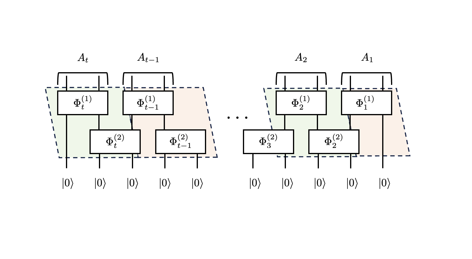
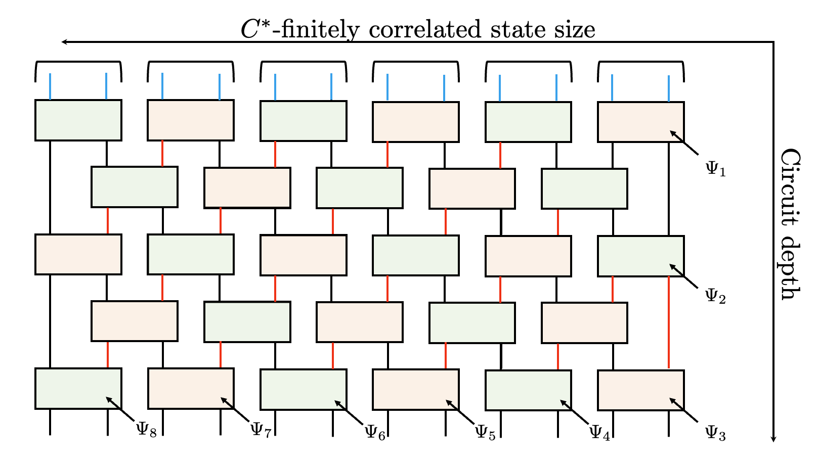
Figure 4: $C^{*}$-finitely correlated description of quantum circuits. On the right figure, the legs in red correspond to the system $\mathcal{B}$ at the entry of a map $\mathcal{E}^{(j)}$, whereas the blue legs correspond to the system $\mathcal{A}$.

In the next section, we consider an important class of many-body quantum states which are known to be approximated by outputs of (non-unitary) circuits as described above, namely

Gibbs states of one-dimensional local Hamiltonians.

6.2 Learning one-dimensional Gibbs states

In the classical setting, Markov chains are known to correspond to finite-size Gibbs measures over spin chains since the seminal paper [34]. This result on the structure of Markov chains was extended to quantum Gibbs states of commuting Hamiltonians in [35]. We recall that, given a local Hamiltonian $H:=\sum_{i=1}^{n-1}h_{i,i+1}\otimes\mathds{1}_{\{i,i+1\}^{c}}\in\mathcal{A}_{[1,n]}$, and an inverse temperature $\beta>0$, the finite-size Gibbs state on $[1,n]$ corresponding to $(H,\beta)$ takes the form

$$\sigma(H,\beta):=\frac{e^{-\beta H}}{\operatorname{Tr}\big{(}e^{-\beta H}\big{)}}\,.$$ (186)

Here, the notion of Markovianity for a quantum state means that, given any tripartition of the finite-size chain into three ordered intervals $ABC$, the quantum conditional mutual information $I(A:C|B)=0$. More recently, Brandao and Kato [36] proved that this equivalence continues to hold approximately in the following sense: a quantum state over a finite spin chain $[1,n]$ is $\epsilon n$-close in relative entropy to the Gibbs state of a nearest-neighbour quantum Hamiltonian iff for any tripartition $ABC$ of the chain, the mutual information is exponentially small in the size $|B|$ of the interval $B$ (see also [37] for extensions to higher dimensions).

The recent years have seen the development of many learning algorithms for Gibbs states. In [29, 38], the authors propose an algorithm based on the maximum entropy optimization problem (maxEnt) whose sample complexity scales polynomially with $n$. However, since maxEnt requires the computation of the partition function of the state, a problem that is known to be NP-hard in general, the method proposed there is not computationally efficient. In contrast, whenever the Hamiltonian is made of commuting terms [39], or when $\beta$ is small enough [40, 41], optimal sample and computational complexities were recovered. We also note that a different approach to the problem was recently proposed by one of the authors, based on the recovery of the distribution in quantum Wasserstein distance [42] instead of that of the interaction matrix. In this framework, optimal sample and computational complexities were obtained for a larger class of Gibbs states satisfying a certain correlation decay property and under a condition of approximate Markov property [43, 44]. Combining the results of [29] and [44], we get a computationally efficient quantum algorithm for learning a classical description $\hat{H}$ of the unknown Hamiltonian $H$ with the guarantee that $\sigma(H,\beta)$ and $\sigma(\hat{H},\beta)$ are $\epsilon$ close in trace distance with probability $1-\delta$, given access to $\mathcal{O}(e^{\beta^{c_{1}}}n^{4}/(\epsilon^{2}\beta^{c_{2}}))\operatorname{polylog}(n/\delta)$ copies of the unknown state $\sigma(H,\beta)$, for some constants $c_{1},c_{2}\geq 1$. In contrast, it was shown in [45, Theorem 1.3] that learning classical Gibbs measures with $\epsilon$ average recovery in trace distance requires at least $n/\epsilon^{2}$ samples. Since classical Gibbs states are finitely correlated states, the latter directly implies the following:

Proposition 6.2.

Let $A$ be a learning algorithm such that, upon measuring $N$ independent copies of an unknown finite-size, finitely correlated state $\rho$ on $\mathcal{A}_{[1,n]}$, outputs an estimated state $\hat{\rho}$ such that $\mathbb{E}\big{[}\|\rho-\hat{\rho}\|_{1}\big{]}\leq\epsilon$, where the expected value refers to the inherent randomness of the measurement outcomes. Then necessarily $N=\Omega(n/\epsilon^{2})$.

Next, we propose a different path for learning one-dimensional Gibbs states in terms of their approximations by matrix product operators. The recent years have significant improvements on the approximation of Gibbs states in terms of matrix product density operators [3, 4, 5].

Unfortunately, the approximated finitely correlated states devised in these works are not manifestly $C^{*}$. In contrast, in [28] the authors constructed a depth two dissipative quasi-local circuit whose output $\widetilde{\sigma}(H,\beta)$ approximates $\sigma(H,\beta)$ in trace distance, essentially by using that such states satisfy (i) exponential decay of correlations, and (ii) exponential decay of the quantum conditional mutual information. It follows from the discussion in Section 6.1 that $\widetilde{\sigma}(H,\beta)$ is a $C^{*}$-finitely correlated state. More precisely, there is a circuit $\mathcal{C}_{H,\beta}$ similar to the left part of Figure 4, albeit with gates acting on $\mathcal{O}(\log(n\epsilon))$, such that

$$\|\mathcal{C}_{H,\beta}(|0^{n}\rangle\langle 0^{n}|)-\sigma(H,\beta)\|_{1}\leq\epsilon\,.$$

By blocking sites together, gates constituting the circuit $\mathcal{C}_{H,\beta}$ can be thought of as acting on two subsystems each, up to replacing the local dimension by $d^{\prime}=(n/\epsilon)^{\mathcal{O}(\log(d))}$. By combining this with Proposition 6.1, we see that our learning algorithm achieves a polynomial sample complexity for the task of learning the reduced states of a Gibbs state at any positive temperature, similarly to that of [29]. However, the degree of the polynomial we achieve with our algorithm in its current state depends on the temperature, and we leave the question of optimizing our procedure to future work.

7 Numerical experiments

7.1 The model: ground state of the AKLT Hamiltonian

In this section, we want to numerically test the performance of Algorithm 1 on a concrete family of $C^{*}$-finitely correlated states that was given in [8] [Section 2, Example 1]. This family of states has the one site observable algebra $\mathcal{A}=\mathbb{M}_{3}$ and is parameterized by a single parameter $\theta\in[0,\pi)$. In order to give the explicit realization we need to define the following linear map

$$V_{\theta}:\mathbb{C}^{2}\rightarrow\mathbb{C}^{3}\otimes\mathbb{C}^{2},$$ (187)

that is completely defined by

$$V_{\theta}|\tfrac{1}{2}\rangle=\cos\theta|1,-\tfrac{1}{2}\rangle-\sin\theta|0,\tfrac{1}{2}\rangle,$$ (188)

$$V_{\theta}|-\tfrac{1}{2}\rangle=\sin\theta|0,-\tfrac{1}{2}\rangle-\cos\theta|-1,\tfrac{1}{2}\rangle,$$ (189)

where $|\pm\frac{1}{2}\rangle$ and $|1\rangle,|0\rangle,|-1\rangle$ denote orthonormal basezs of $\mathbb{C}^{2}$ and $\mathbb{C}^{3}$ respectively. Then the states $w_{\theta}$ that we consider are given by the realization $(\mathcal{V},e,\mathbb{E}_{\theta},\rho)$ described by,

• $\mathcal{V}=\mathbb{M}_{2}$.

• $\mathbb{E}_{\theta,A}(B)=V^{*}_{\theta}(A\otimes B)V_{\theta}$ for $A\in\mathbb{M}_{3}$ and $B\in\mathbb{M}_{2}$.

• $\rho(B)=\frac{1}{2}\operatorname{Tr}(B)$ for $B\in\mathbb{M}_{2}$.

• $e=\mathds{1}_{\mathbb{M}_{2}}\in\mathbb{M}_{2}$.

Thus, for any translation invariant state $w_{\theta}$ described by the above realization, we can recover any correlation function as

$$\omega_{\theta}(A_{1}\otimes\cdots\otimes A_{k})=\frac{1}{2}\operatorname{Tr}\left(\mathbb{E}_{\theta,A_{k}}\cdots\mathbb{E}_{\theta,A_{1}}(\mathds{1})\right),$$ (190)

for any $A_{1},\dots,A_{k}\in\mathbb{M}_{2}$. This family of states is interesting because for the particular value of $\cos\theta=\sqrt{\frac{2}{3}}$ the state $w_{\theta}$ coincides with the ground state of the AKLT Hamiltonian introduced in [46] and given by

$$H_{\text{aklt}}=\sum_{i}\frac{1}{2}\mathbf{S}_{i}\cdot\mathbf{S}_{i+1}+\frac{1}{6}\left(\mathbf{S}_{i}\cdot\mathbf{S}_{i+1}\right)^{2}+\frac{1}{3},$$ (191)

where $\mathbf{S}_{i}=(S_{x},S_{y},S_{z})$ denote the spin 1 irreducible representation of $SU(2)$ acting at site $i$.

7.2 Results

For the simulations, we restrict our attention to the ground state of the AKLT Hamiltonian (191) and fix $\cos\theta=\sqrt{\frac{2}{3}}$ in the realization of the previous Section 7.1. In order to fix a basis for the one site algebra $\mathbb{M}_{3}$ we use the normalized Gell-Mann matrices $\{\lambda_{i}\}_{i=0}^{8}$ (see Appendix E) where $\lambda_{0}$ is the normalized identity such that $\operatorname{Tr}(\lambda_{i}\lambda_{j})=\delta_{i,j}$. We are interested in recovering the reduced density matrices of $k$ contiguous sites that are described by

$$\rho^{k}_{\theta}=\sum_{i_{1},\dots,i_{k}}\omega_{\theta}(\lambda_{i_{1}}\otimes\cdots\otimes\lambda_{i_{k}})\lambda_{i_{1}}\otimes\cdots\otimes\lambda_{i_{k}},$$ (192)

where $i_{1},\dots,i_{k}\in\{0,1,\dots,8\}^{\otimes k}$. For the observable regular realization (Proposition 2.5), we fix the right and left finite-dimensional unital subalgebras $\mathcal{C}_{R}=\mathcal{C}_{L}=\mathbb{M}_{3}$ for two contiguous sites with basis $\{\lambda_{i}\}_{i=0}^{8}$ for both $\mathcal{C}_{R}$ and $\mathcal{C}_{L}$. In order to test our algorithm, we will use some simulated data. Specifically, since we have access to the realization (7.1) we can compute the maps $\Omega$ and $\Omega_{A}$ for $A\in\{\lambda_{i}\}_{i=0}^{8}$ which are the observables that we want to read from the experiment. For completeness, we numerically check that $\text{rank}(\Omega)=4$ which is consistent with the realization given in Section 7.1 since $\text{dim}(\mathcal{V})=4$. Then we fix the errors $\epsilon,\epsilon^{\prime}>0$ and generate the simulated observables $\hat{\Omega}$ and $\hat{\Omega}_{A}$ as follows

$$\hat{\Omega}=\Omega+\epsilon\frac{P}{\|P\|_{2}}\quad\hat{\Omega}_{\lambda_{i}}=\hat{\Omega}_{\lambda_{i}}+\epsilon^{\prime}\frac{P^{\prime}_{i}}{\|P\|_{2}},$$ (193)

for all $i=0,\dots,8$ and $P,P_{i}^{\prime}\in\mathbb{R}^{9\times 9}$ are matrices where each entry is drawn from a Gaussian distribution with zero mean and unit variance. With this construction, we can fix the errors $\|\Omega-\hat{\Omega}\|_{2}$ and $\|\Omega-\hat{\Omega}_{(\cdot)}\|_{2}$. Given the singular value decomposition of $\hat{\Omega}$ we need to achieve the invertibility condition of Theorem 4.3 that says that $\hat{U}^{\intercal}U$ is invertible. In general $\hat{U}^{\intercal}\in\mathbb{R}^{9\times 9}$ since the perturbation $P$ will make $\hat{\Omega}$ full rank. In order to avoid this issue we can use as input rank $m=4$ and we truncate $\hat{U}$ such that we keep the columns corresponding to the 4 largest singular values of $\hat{\Omega}$. Another possibility is to use Lemma B.1 in order to justify that the singular values with absolute values smaller than a precision $\eta$ can not be distinguished from 0. Thus, setting $\eta$ small enough following conditions in Theorem 1.2 we can truncate $\hat{U}$ keeping the columns corresponding to singular values greater than the precision $\eta$.

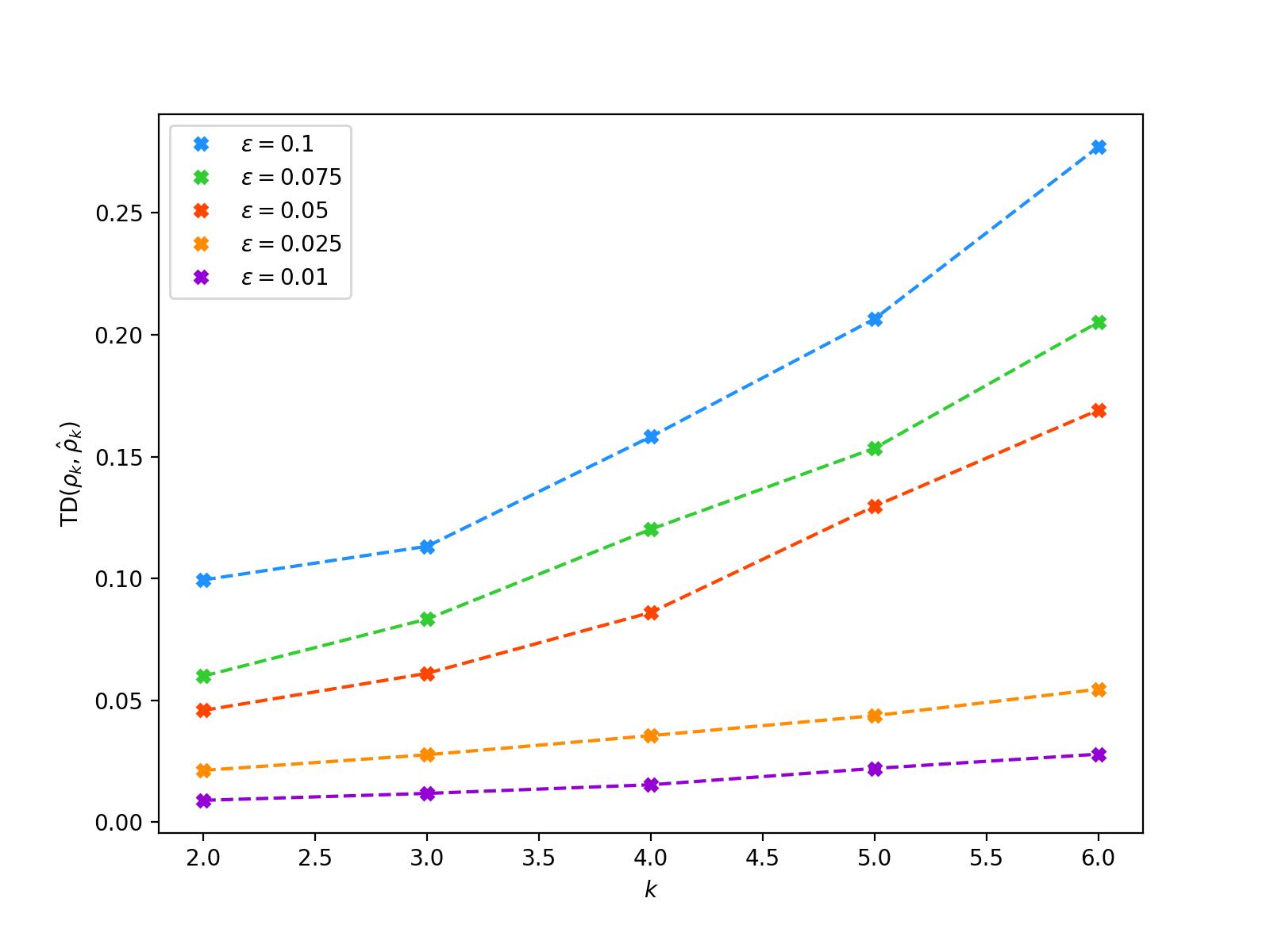
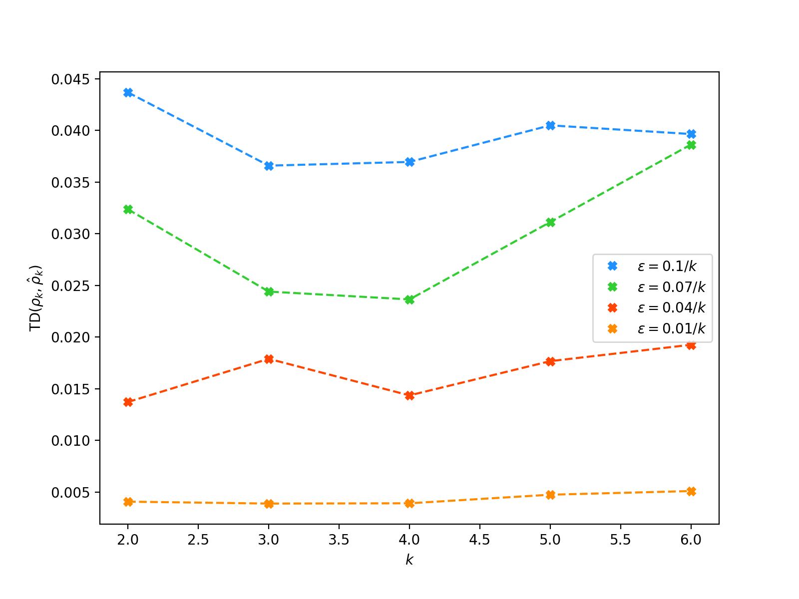
Figure 5: Scaling of trace distance $\text{TD}(\rho_{k},\hat{\rho}_{k})=\frac{1}{2}\|\rho_{k}-\hat{\rho}_{k}\|_{1}$ between the true reduced density matrix $\rho_{k}$ of the ground state of the AKLT model and the reconstructed one $\hat{\rho}_{k}$ from the maps $\hat{\Omega},\hat{\Omega}_{(\cdot)}$. We study the scaling for different errors $\epsilon=\|\hat{\Omega}-\Omega\|_{2}=\|\hat{\Omega}_{(\cdot)}-\Omega_{(\cdot)}\|_{2}$ where $\lambda_{i}$ are the normalized basis elements of the one site algebra $\mathbb{M}_{3}$. Left plot: each line corresponds to a fixed $\epsilon$ and the reconstruction of $\rho_{k}$ is done using the same $\hat{\Omega},\hat{\Omega}_{(\cdot)}$. This plot illustrates the exponential behavior of the error propagation Theorem 4.5 coming from the factor $(1+\Delta)^{t}$. Right plot: each dot corresponds to an independent experiment and the error is normalized by the number of sites. This plot illustrates the linear behavior if we renormalize the errors since $(1+\Delta/k)^{k}\leq 1+2k$ (for $\Delta\leq 1/2$).

Using the simulated observables $\hat{\Omega},\hat{\Omega}_{\lambda_{i}}$ and the truncated $\hat{U}$ we use the spectral state decomposition of Definition 4.1 and compute the correlations

$$\hat{\omega}_{\theta}(\lambda_{i_{1}}\otimes\cdots\otimes\lambda_{i_{k}})=\hat{\rho}\hat{\mathbb{K}}_{\lambda_{i_{1}}}\cdots\hat{\mathbb{K}}_{\lambda_{i_{k}}}\hat{e},$$ (194)

for different numbers of sites $k$. Then we reconstruct the full state $\hat{\rho}_{k}$ as in (192) replacing $\omega_{\theta}$ by $\hat{\omega}_{\theta}$. Finally we compute the trace distance $\frac{1}{2}\|\hat{\rho}_{k}-\rho_{k}\|_{1}$ and plot our results in Figure 5.

Appendix A Operator systems and completely bounded norms

The memory system $V$ of a finitely correlated state $\omega$ on $\mathcal{A}$ with regular realization $(V,e,\mathbb{E},\rho)$ inherits the structure of an operator system [8, Lem. A.1]. In brief, it is constructed from the positivity structure on $\mathbb{M}_{n}(\mathcal{A})$ by push-forward with the map $\Psi:\mathcal{A}_{R}\to V$ and its amplifications.

We will summarize some facts about the theory of operator systems in this section. For more details see [26].

Definition A.1.

Let $V$ be a complex vector space with a (conjugate-linear) involution $*:V\to V$ and a family $C$ of cones $C_{n}\subset\mathbb{M}_{n}(V)\cong\mathbb{M}_{n}\otimes V$ defining an order on $\mathbb{M}_{n}(V)$. We then obtain a natural involution on $\mathbb{M}_{n}(V)$. Let $e\in V$. We call $V\equiv(V,C,e)$ an (abstract) operator system if the following are satisfied

1. Each $X\in C_{n}$ is self-adjoint.

2. $e$ is an Archimedean matrix order unit for the cones $C_{n}$.

3. For each $k\times n$-matrix $M\in\mathbb{M}_{k,n}$ it holds that $M^{*}C_{k}M\subset C_{n}$.

Since $e$ is a matrix order unit, by definition for every $n$ and every self-adjoint $X\in\mathbb{M}_{n}(V)$ there exists $r>0$ such that $re^{(n)}\geq X$ where $e^{(n)}=\mathds{1}_{\mathbb{M}_{n}}\otimes e$. For $X\in\mathbb{M}_{n}(V)$ let

$$S(X)=\begin{pmatrix}0&X\\ X^{*}&0\end{pmatrix}.$$

Note that $S(X)=S(X)^{*}$. The order norm of $X\in\mathbb{M}_{n}(V)$ is then defined as

$$\|X\|_{e^{(n)}}=\inf\{r\in\mathbb{R}_{+}\ |\ re^{(2n)}\geq S(X)\}\geq 0.$$

$e$ being Archimedean implies that the order norms are, in fact, norms and that the corresponding cones are closed. For self-adjoint $X$ the order norm is also given as $\|X\|_{e^{(n)}}=\inf\{r>0\ |\ re^{(n)}\geq X,-X\}$. It always holds that $\|e^{(n)}\|_{e^{(n)}}=1$. For a linear map $\alpha:V\to W$ between operator systems we denote its $n$-th amplification by $\alpha_{n}=\mathrm{id}_{\mathbb{M}_{n}}\otimes\ \alpha:\mathbb{M}_{n}(V)\to\mathbb{M}_{n}(W)$. $\alpha$ is called positive if it maps positive elements of $V$ to positive elements of $W$ and completely positive if each of its amplifications is positive. We then write $\alpha\in\mathrm{CP}(V,W)$. It is unital if it maps the order unit of $V$ to the order unit of $W$. If $\alpha$ is completely positive then $\alpha$ is bounded with its operator norm satisfying $\|\alpha\|=\|\alpha(e_{V})\|_{e_{W}}$. The Choi-Effros theorem [26, Thm. 13.1] ensures that every abstract operator system can be represented faithfully as a concrete operator system, meaning a $*$-invariant subspace of $\mathcal{B}(\mathcal{H})$ for some Hilbert space $\mathcal{H}$.

The estimates in Section 4 also require us to use norms of complete boundedness. The natural setting for talking about these norms is that of an operator space, that is a closed subspace of $\mathcal{B}(\mathcal{H})$. For more information see [47]. There is an abstract characterization of this structure, similar to the abstract characterization of operator systems above, such that every abstract operator space can be represented as a concrete operator space by Ruan’s theorem [26, Thm. 13.4]. The structure of an (abstract) operator system induces the structure of an (abstract) operator space. A linear map $\alpha:V\to W$ between operator spaces is called completely bounded if all its amplifications $\alpha_{n}$ are bounded and the sequence of operator norms $\|\alpha_{n}\|$ is uniformly bounded. The corresponding norm of complete boundedness is then

$$\|\alpha\|_{cb}\equiv\|\alpha\|_{\mathrm{CB}(V,W)}=\sup_{n}\|\alpha_{n}\|_{\mathcal{B}(\mathbb{M}_{n}(V),\mathbb{M}_{n}(W))}.$$

If $\alpha$ is a completely positive map between operator systems then $\|\alpha\|_{cb}=\|\alpha\|=\|\alpha(e_{V})\|_{e_{W}}$. If $\alpha$ is unital it is thus automatically completely contractive. Furthermore, the following bound is true [47, Thm. 3.8]:

Lemma A.2.

If $\alpha$ has rank $m$ then $\|{\alpha}\|_{\mathrm{CB}(V,W)}\leq m\|\alpha\|_{\mathcal{B}(V,W)}$. In particular, this is the case whenever $V$ or $W$ is finite-dimensional.

We also have the following result. It is basically [47, Prop. 1.12] which is valid also for abstract operator spaces by Ruan’s theorem.

Lemma A.3.

If $\alpha$ is a map from an (abstract) operator space $V$ to $\mathbb{M}_{n}$, then $\|{\alpha}\|_{cb}=\|\alpha_{n}\|_{\mathcal{B}(\mathbb{M}_{n}(V),\mathbb{M}_{n^{2}})}$.

Remark A.4.

While there is a clear link between the structures of operator systems and operator spaces, the corresponding categories do not behave exactly the same. For example, the natural operator system structure induced on the quotient of an operator system does not in general coincide with the quotient operator space structure. A second subtlety concerns conventions in the literature. Concrete operator systems and, in particular, spaces are often assumed to be closed (hence complete) in norm. For the abstract structures, in particular operator systems, this is often not required (and then also not true when represented faithfully). This is certainly not a real problem in practice but should be kept in mind to avoid confusion. Both subtleties are illustrated by [48, Prop. 4.5].

Let $\mathcal{H}$ be a Hilbert space. Then there exists a natural operator space structure on $\mathcal{H}$ satisfying that the (conjugate linear) identification $\mathbb{M}_{n}(\mathcal{H})\cong\mathbb{M}_{n}(\mathcal{H})^{*}$ is completely isometric [47, Ch. 7]. We will implicitly use this operator system structure whenever we talk about complete boundedness of maps on Hilbert spaces. It holds [47, Prop. 7.2]:

Lemma A.5.

If $\mathcal{H}$ and $\mathcal{K}$ are Hilbert spaces and $T\in\mathcal{B}(\mathcal{H},\mathcal{K})$ then $\|T\|_{cb}=\|T\|$.

Appendix B Matrix perturbation theory

We list the matrix perturbation theory results that we use, following the analysis of [12, 18, 19].

Lemma B.1 (Theorem 4.11, in [49], p.204).

Let $A,\tilde{A}\in\mathbb{R}^{m\times n}$ with $n\leq m$. Then if $\sigma_{1}\geq\cdots\geq\sigma_{n}$ and $\tilde{\sigma}_{1}\geq\cdots\geq\tilde{\sigma}_{n}$ are the singular values of $A$ and $A^{\prime}$ respectively then

$$|\sigma_{i}-\tilde{\sigma}_{i}|\leq\|A-\tilde{A}\|_{2}\quad\text{for}\quad i=1,\dots,n.$$ (195)

Lemma B.2 (Theorem 3.8 in [49], p.143).

Let $A,\tilde{A}\in\mathbb{R}^{m\times n}$, then the error for the pseudo-inverses has the following bound

$$\|\tilde{A}^{+}-A^{+}\|_{2\rightarrow 2}\leq\frac{1+\sqrt{5}}{2}\max\{\|\tilde{A}^{+}\|^{2}_{2\rightarrow 2},\|A^{+}\|^{2}_{2\rightarrow 2}\}\|\tilde{A}-A\|_{2\rightarrow 2}.$$ (196)

The following perturbation bounds can be found in [49].

Lemma B.3 (Corollary 17 of [18]).

Let $A\in\mathbb{R}^{m\times n}$, with $m\geq n$, have rank $n$, and let $U\in\mathbb{R}^{m\times n}$ be the matrix of $n$ left singular vectors corresponding to the non-zero singular values $\sigma_{1}\geq\ldots\geq\sigma_{n}>0$ of $A$. Let $\tilde{A}=A+E$. Let $\tilde{U}\in\mathbb{R}^{m\times n}$ be the matrix of $n$ left singular vectors corresponding to the largest $n$ singular values $\tilde{\sigma}_{1}\geq\ldots\geq\tilde{\sigma}_{n}$ of $\tilde{A}$, and let $\tilde{U}_{\perp}\in\mathbb{R}^{m\times(m-n)}$ be the remaining left singular vectors. Assume $\|E\|_{2}\leq\epsilon\sigma_{n}$ for some $\epsilon<1$. Then:

1. $\tilde{\sigma}_{n}\geq(1-\epsilon)\sigma_{n}$,

2. $\|\tilde{U}_{\perp}^{\intercal}U\|_{2}\leq\|E\|_{2}/\tilde{\sigma}_{n}$.

Lemma B.4.

[Special case of Corollary 2.4 of  [50]] Let $A\in\mathbb{R}^{d_{1}\times d_{2}}$ of rank $m$, and $S\in\mathbb{R}^{d_{1}\times d_{1}}$, $T\in\mathbb{R}^{d_{2}\times d_{2}}$. Then, for any $1\leq i\leq m$

$$\sigma_{d_{1}}(S)\sigma_{d_{1}}(T)\leq\frac{\sigma_{i}(SAT)}{\sigma_{i}(A)}\leq\sigma_{i}(S)\sigma_{i}(T)$$ (197)

Lemma B.5.

In the notations of Section 4, suppose $\|\Omega-\hat{\Omega}\|_{2}\leq\varepsilon\cdot\sigma_{m}(\Omega)$ for some $\varepsilon<1/2$. Then $\varepsilon_{0}:=\|\Omega-\hat{\Omega}\|_{2}^{2}/((1-\varepsilon)\sigma_{m}(\Omega))^{2}<1$ and:

1. $\sigma_{m}(\hat{U}^{\intercal}\hat{\Omega})\geq(1-\varepsilon)\sigma_{m}(\Omega)$,

2. $\sigma_{m}(\hat{U}^{\intercal}U)\geq\sqrt{1-\varepsilon_{0}}$,

3. $\sigma_{m}(\hat{U}^{\intercal}\Omega)\geq\sqrt{1-\varepsilon_{0}}\sigma_{m}(\Omega)$.

Proof.

Since $\sigma_{m}(\hat{U}^{\intercal}\hat{\Omega})=\sigma_{m}(\hat{\Omega})$, the second claim is immediate from Lemma B.3. 3. follows since for any $x\in\mathbb{C}^{m}$, $\|\hat{U}^{\intercal}Ux\|_{2}\geq\|x\|_{2}\sqrt{1-\|\hat{U}_{\perp}^{\intercal}U\|_{2}^{2}}\geq\|x\|_{2}\sqrt{1-\varepsilon_{0}}$ by Lemma B.3 and the fact that $\varepsilon_{0}<1$ (see Lemma 21 of [18] for a full proof). The remaining claims follow from Lemma B.4 noticing that $\sigma_{m}(\hat{U}\Omega)=\sigma_{m}((\hat{U}U)(U^{\intercal}\Omega))$, $\sigma_{m}(U\Omega)=\sigma_{m}(\Omega)$, so that we have 4. choosing $S=\hat{U}^{\intercal}U$, and $AT$ be the polar decomposition of $U^{\intercal}\Omega$. ∎

Appendix C Proofs for the non-homogeneous case

C.1 Proof of Proposition 5.2

Proposition.

Defining

$${\mathbb{K}}^{(1)}_{A} =(\Omega_{A}^{[1,0,1+r]})({{U}_{1}}^{\intercal}\Omega^{[1,1,1+r]})^{+},$$ (198)

$${\mathbb{K}}^{(N)}_{A} ={{U}}^{\intercal}_{N-1}(\Omega_{A}^{[N-l,N-1,N]}),$$ (199)

$$\mathbb{K}^{(j)}_{X_{j}} :=U_{j-1}^{\intercal}\Omega^{[j-l,j-1,j+r]}_{X_{j}}(U_{j}^{\intercal}\Omega^{[j-l+1,j,j+r]})^{+},\mathrm{for}\,2\leq j\leq N-1$$ (200)

we have

$$\omega(X_{1}\otimes\cdots\otimes X_{N}) =\mathbb{K}_{X_{1}}^{(1)}\cdots\mathbb{K}_{X_{N}}^{(N)}.$$ (201)

Proof.

For $1\leq i,j\leq N$, let $V_{[i+1,j]}$ be the space generated by the span of the functionals $\Psi^{(i,j)}_{X}\in\mathcal{A}_{[\max(1,i-l+1),\min(i,N)]}^{*}$, $X\in\mathcal{A}_{[\max(1,i+1),\min(j,N)]}$, $\Psi^{(i,j)}_{X}(Y):=\omega(Y\otimes X)$ (where $V_{[N+1,N]}$ is one-dimensional and it is the span of the functional $\Psi(Y)=\omega(\mathds{1}\otimes Y)$, $Y\in\mathcal{A}_{[N-r,N]}$, and $V_{[1,j]}$ is one-dimensional as it is the span of functionals $\Phi(X)=\omega(X)$, $X\in\mathcal{A}_{[1,j]}$ also on a one-dimensional vector space). For $i=1,...,N$ we can define the linear maps $\mathbb{E}_{A}^{(i)}:V_{[i+1,i+r+1]}\rightarrow V_{[i,i+r]}$ as $\mathbb{E}^{(i)}_{A}\Psi^{(i+1,i+r+1)}_{X}=\Psi^{(i,i+r+1)}_{A\otimes X}=\Psi^{(i,i+r)}_{X^{\prime}}$, where the last equality holds for some $X^{\prime}\in A_{[\max(1,i+1),\min(N,i+r)]}$ because of the definition of $(l,r,m)$-finitely correlated state. We obtain

$$\omega(X_{1}\otimes\cdots\otimes X_{N})=\mathbb{E}_{X_{1}}^{(1)}\cdots\mathbb{E}_{X_{N}}^{(N)}.$$ (202)

The image of $\Omega^{[j-l+1,j,j+r]}$ lies in $V_{[j+1,j+r]}$, so we can write

$$\mathbb{E}_{X_{j}}^{(j)}\Omega^{[j-l+1,j,j+r]}=\Omega^{[j-l,j-1,j+r]}_{X_{j}},$$ (203)

where $\Omega^{[j-l,j-1,j+r]}_{X_{j}}:\mathcal{A}_{[j,\min(j+r,N)]}\rightarrow V_{[j,j+r+1]}=V_{[j,j+r]}$, $\Omega^{[j-l,j-1,j+r]}_{X_{j}}(X)=\Psi^{(j,j+r+1)}_{X_{j}\otimes X}$. Using the singular value decomposition

$$\Omega^{[j-l+1,j,j+r]}={{U}}_{j}D_{j}{W}_{j}^{\intercal},$$ (204)

with $U_{j}:\mathbb{R}^{m_{j}}\rightarrow V_{[j,j+r]}$, $D:\mathbb{R}^{m_{j}}\rightarrow\mathbb{R}^{m_{j}}$, $W_{j}^{\intercal}:\mathcal{A}_{[j+1,j+r]}\rightarrow\mathbb{R}^{m_{j}}$. We get

$$\mathbb{E}_{X_{N}}^{(N)} =\Omega^{[N-l,N-1,n+r]}_{X_{N}}$$ (205)

$$\mathbb{E}_{X_{j}}^{(j)}{U}_{j} =\Omega^{[j-l,j-1,j+r]}_{X_{j}}({U}_{j}^{\intercal}\Omega^{[j-l+1,j,j+r]})^{+}$$ (206)

Note that for $X\in A_{[j+1,j+r]}$, ${U}_{j}{U}_{j}^{\intercal}\Psi^{[j,j+r]}_{X}={U}_{j}{U}_{j}^{\intercal}\Omega^{[j-l+1,j,j+r]}(X)=\Omega^{[j-l+1,j,j+r]}(X)=\Psi^{[j,j+r]}_{X}$, therefore we have

$$\omega(X_{1}\otimes\cdots\otimes X_{n}) =\mathbb{K}_{X_{1}}^{(1)}\cdots\mathbb{K}_{X_{N}}^{(N)}.$$ (207)

∎

C.2 Proof of Proposition 5.8

Proposition.

For an observable realization as in Definition 5.2, and a realization as in Definiton 5.7, we have

$${\mathbb{K}}^{(1)}_{A}{U}_{1}^{\intercal}\mathcal{F}_{1}|_{\mathcal{W}_{1}} =\mathcal{F}_{0}\mathcal{E}_{A}^{(1)}|_{\mathcal{W}_{1}},$$ (208)

$${\mathbb{K}}^{(N)}_{A} ={U}_{N-1}^{\intercal}\mathcal{F}_{N-1}\mathcal{E}_{A}^{(N)}(\mathds{1}_{B}),$$ (209)

$${\mathbb{K}}^{(j)}_{A}{U}_{j}^{\intercal}\mathcal{F}_{j}|_{\mathcal{W}_{j}} ={U}_{j-1}^{\intercal}\mathcal{F}_{j-1}\mathcal{E}_{A}^{(j)}|_{\mathcal{W}_{j}},\mathrm{for}\,2\leq j\leq N-1,$$ (210)

and

$${\mathbb{K}}^{[j,N]}_{X_{1}\otimes\cdots\otimes X_{N}} ={U}_{j-1}^{\intercal}\mathcal{F}_{j-1}\mathcal{E}^{[j,N]}_{X_{1}\otimes\cdots\otimes X_{N}}(\mathds{1}_{\mathcal{B}}),\mathrm{for}\,2\leq j\leq N-1,$$ (211)

$${\mathbb{K}}^{[1,N]}_{X_{1}\otimes\cdots\otimes X_{N}} =\rho_{0}\mathcal{E}^{[1,N]}_{X_{1}\otimes\cdots\otimes X_{N}}(\mathds{1}_{\mathcal{B}}).$$ (212)

Let us define the linear maps $\mathcal{E}^{[i,j]}:\mathcal{A}_{{i,j}}\otimes\mathcal{B}\rightarrow\mathcal{B}$ which act on a product vector $X_{j}\otimes\cdots\otimes X_{k}\otimes Z$ as

$$\mathcal{E}^{[i,j]}(X_{i}\otimes\cdots\otimes X_{j})=\mathcal{E}_{X_{j}}^{(j)}\cdots\mathcal{E}_{X_{k}}^{(k)}(Z).$$ (213)

For $C^{*}$-finitely correlated state we can write

$$\omega(X_{1}\otimes\cdots\otimes X_{N}) =\rho_{0}{\mathcal{E}_{X_{1}}^{(1)}}\cdots{\mathcal{E}_{X_{N}}^{(N)}}(\mathds{1}_{\mathcal{B}})=\rho_{0}\mathcal{E}^{[1,N]}(X_{1}\otimes\cdots\otimes X_{N}\otimes\mathds{1}_{\mathcal{B}}),$$ (214)

and defining $\rho_{i-1}:=\rho_{0}{\mathcal{E}_{\mathds{1}}^{(1)}}\cdots{\mathcal{E}_{\mathds{1}}^{(i-1)}}$ we see

$$\Omega^{[i,j,k]}[X_{i}\otimes\cdots\otimes X_{j}](X_{j+1}\otimes\cdots\otimes X_{k})=(\mathcal{E}_{X_{i}}^{(i)}\cdots\mathcal{E}_{X_{j}}^{(j)})^{\dagger}(\rho_{i-1})(\mathcal{E}_{X_{j+1}}^{(j+1)}\cdots{\mathcal{E}_{X_{k}}^{(k)}}(\mathds{1}))$$ (215)

First we prove the following:

Lemma C.1.

$U^{\intercal}_{j}\mathcal{F}_{j}$ is invertible on $\mathcal{V}^{\prime}_{j}$.

Proof.

We have that for $A\in\mathcal{A}_{[j+1,j+r]}$ such that $0\neq\mathcal{E}^{[j,j+r]}(A\otimes\mathds{1}_{\mathcal{B}})\in\mathcal{V}^{\prime}_{j}$, there exists $A^{\prime}\in\mathcal{A}_{[j-l+1,j]}$ such that

$$\rho_{j-l+1}\mathcal{E}^{[j-l+1,j]}(A^{\prime}\otimes\mathcal{E}^{[j+1,j+r]}(A\otimes\mathds{1}_{\mathcal{B}}) =\Omega^{[j-l+1,j,j+r]}[A](A^{\prime})=U_{j}D_{j}O_{j}[A](A^{\prime})\neq 0,$$ (216)

implying $O_{j}[A]\neq 0$. Thus we have

$$U_{j}^{\intercal}\mathcal{F}_{j}(\mathcal{E}^{[j+1,j+r]}(A\otimes\mathds{1}_{\mathcal{B}})) =U_{j}^{\intercal}\Omega^{[j-l+1,j,j+r]}[A]=D_{j}O_{j}[A]\neq 0.$$ (217)

∎

Then we can prove Proposition 5.8

Proof.

We have, for any $X_{j+1}\otimes\cdots\otimes X_{j+r}\in\mathcal{A}_{[j+1,j+r]}$, $X_{j-l-1}\otimes\cdots\otimes X_{j}\in\mathcal{A}_{[j-l+1,j]}$,

$$\mathcal{F}_{j}[\mathcal{E}_{X_{j+1}}^{(j+1)}\cdots{\mathcal{E}_{X_{j+r}}^{(j+r)}}(\mathds{1})](X_{j-l+1}\otimes\cdots\otimes X_{j})=\rho_{j-l}\mathcal{E}_{X_{j-l+1}}^{(j-l-1)}\cdots\mathcal{E}_{X_{j}}^{(j)}\mathcal{E}_{X_{(j+1)}}^{(j+1)}\cdots{\mathcal{E}_{X_{j+r}}^{(j+r)}}(\mathds{1}),$$ (218)

in particular

$$\mathcal{F}_{j}[\mathcal{E}_{X_{j+1}}^{(j+1)}\cdots{\mathcal{E}_{X_{(j+r)}}^{(j+r)}}(\mathds{1})](X_{j-l+1}\otimes\cdots\otimes X_{j})=\Omega^{[j-l+1,j,j+r]}[X_{j+1}\otimes\cdots\otimes X_{j+r}](X_{j-l+1}\otimes\cdots\otimes X_{j}),$$ (219)

and

$$\mathcal{F}_{j-1}[\mathcal{E}_{X_{j}}^{(j)}\mathcal{E}_{X_{j+1}}^{(j+1)}\cdots{\mathcal{E}_{X_{k}}^{(j+r)}}(\mathds{1})](X_{j-l}\otimes\cdots\otimes X_{j-1})=\Omega^{[j-l,j-1,j+r]}_{X_{j}}[X_{j+1}\otimes\cdots\otimes X_{j+r}](X_{j-l}\otimes\cdots\otimes X_{j-1}),$$ (220)

Writing $(U^{\intercal}_{j}\mathcal{F}_{j})^{-1}$ for the inverse of $U^{\intercal}_{j}\mathcal{F}_{j}$ on $\mathcal{V}^{\prime}_{j}\subseteq\mathcal{W}_{j}$, for $2\leq j\leq N-1$ we have

$$\mathbb{K}^{(j)}_{A}(x) :=U_{j-1}^{\intercal}\mathcal{F}_{j-1}\mathcal{E}^{[j,j+r]}(A\otimes(U^{\intercal}_{j}\Omega^{[j-l+1,j,j+r]})^{+}(x)\otimes\mathds{1}_{\mathcal{B}})$$ (221)

$$=U_{j-1}^{\intercal}\mathcal{F}_{j-1}\mathcal{E}^{(j)}_{A}(\mathcal{E}^{[j+1,j+r]}((U^{\intercal}_{j}\Omega^{[j-l+1,j,j+r]})^{+}(x)\otimes\mathds{1}_{\mathcal{B}}))$$ (222)

$$=U_{j-1}^{\intercal}\mathcal{F}_{j-1}\mathcal{E}^{(j)}_{A}((U^{\intercal}_{j}\mathcal{F}_{j})^{-1}U^{\intercal}_{j}\mathcal{F}_{j}\mathcal{E}^{[j+1,j+r]}((U_{j}^{\intercal}\Omega^{[j-l+1,j,j+r]})^{+}(x)\otimes\mathds{1}))$$ (223)

$$=U_{j-1}^{\intercal}\mathcal{F}_{j-1}\mathcal{E}^{(j)}_{A}(U^{\intercal}_{j}\mathcal{F}_{j})^{-1}(x),$$ (224)

and similarly for $j=1$ and $j=N$. The rest follows by composition.

∎

Appendix D Guarantees on marginal size for translation invariant states

We observe that if the rank $m$ of the finitely correlated state viewed as a bilinear form is known, the construction can be made completely explicit. First, we have the following lemma.

Lemma D.1.

Define $V_{i}$ the vector space generated by functionals $\Psi_{X}:\mathcal{A}_{L}\rightarrow\mathbb{C}$ of the form

$$\Psi_{X}(A_{1}\otimes\cdots\otimes A_{n}):=\omega(X\otimes A_{1}\otimes\cdots\otimes A_{n}),$$ (225)

with $X\in\mathcal{A}_{[-i+1,0]}$ and $n\in\mathbb{N}$. If $\omega$ has a minimal realization of dimension $m$, then there exists $i\leq m$ such that $V_{i}=V_{j}=\Psi(\mathcal{A}_{R})$ for each $j\geq i$. In particular, this holds for $V_{m}$.

Proof.

Let $i$ be such that $\dim V_{i}=\dim V_{i+1}$, i.e. $V_{i}=V_{i+1}$. Let $\Psi_{Y_{k}}$, $k=1,\dots,\dim V_{i}$, be a basis of $V_{i}$, so $Y_{k}\in\mathcal{A}_{[-i+1,0]}$. If $X=\sum_{j}X_{j}\otimes A_{j}\in\mathcal{A}_{[-i-1,-1]}\otimes\mathcal{A}=\mathcal{A}_{[-i-1,0]}$, i.e. $\Psi_{X}\in V_{i+2}$, then for $A\in\mathcal{A}_{R}$ using translation invariance of the FCS $\omega$:

$$\Psi_{X}(A)=\sum_{j}\Psi_{X_{j}}(A_{j}\otimes A)=\sum_{j,k}c_{jk}\Psi_{Y_{k}}(A_{j}\otimes A)=\sum_{j,k}c_{jk}\Psi_{Y_{k}\otimes A_{j}}(A)=\Psi_{Y}(A)$$

where $Y=\sum_{j,k}c_{jk}Y_{k}\otimes A_{j}\in\mathcal{A}_{[-i,0]}$. Therefore, $V_{i+2}=V_{i+1}$ and by induction $V_{i}=V_{j}=\Psi(\mathcal{A}_{L})$ for all $j\geq i$. Because of $\dim(\Psi(\mathcal{A}_{L}))=m$ by assumption, we have $\dim V_{i}=m$ and thus $i\leq m$ since $\dim V_{j}$ has to increase monotonically in $j$. ∎

Let $\Phi:\mathcal{A}_{L}\to\mathcal{A}_{[1,m]}^{*}$ be the map such that $\Phi_{X}(Y)=\Psi_{Y}(X)$ where $X\in\mathcal{A}_{L},Y\in\mathcal{A}_{[1,m]}$. Furthermore, $\Phi(\mathcal{A}_{L})\cong\Psi(\mathcal{A}_{R})^{*}\cong\Psi(\mathcal{A}_{[1,m]})^{*}$, and vice versa, the last being through because of the above Lemma. The argument in the proof of the above Lemma can also be applied to the analogous spaces $W_{i}$ for $\Phi$ showing that $\Phi(\mathcal{A}_{L})\cong\Phi(\mathcal{A}_{[-m+1,0]})$.

Therefore, it suffices to parametrize $\Psi_{X}$ by $X\in\mathcal{A}_{[1,m]}$ and restrict to $\mathcal{A}_{[-m+1,0]}$ so one has

Corollary D.2.

Define $V_{i,j}$ the vector space generated by functionals $\Psi_{X}:\mathcal{A}_{[-j+1,0]}\rightarrow\mathbb{C}$ of the form

$$\Psi_{X}(A):=\omega(X\otimes A),$$ (226)

with $X\in\mathcal{A}_{[1,i]}$. If $\omega$ has a minimal realization of dimension $m$, $V_{m,m}$ has dimension $m$. The same result holds for the analogously defined spaces $W_{i,j}$ of functionals on the left-hand side of the chain.

Appendix E Normalized Gell-Mann matrices

$$\lambda_{0}=\frac{1}{\sqrt{3}}\begin{pmatrix}1&0&0\\ 0&1&0\\ 0&0&1\end{pmatrix}\quad\lambda_{1}=\frac{1}{\sqrt{2}}\begin{pmatrix}0&1&0\\ 1&0&0\\ 0&0&0\end{pmatrix}\quad\lambda_{2}=\frac{1}{\sqrt{2}}\begin{pmatrix}0&-i&0\\ i&0&0\\ 0&0&0\end{pmatrix}$$

$$\lambda_{3}=\frac{1}{\sqrt{2}}\begin{pmatrix}1&0&0\\ 0&-1&0\\ 0&0&0\end{pmatrix}\quad\lambda_{4}=\frac{1}{\sqrt{2}}\begin{pmatrix}0&0&1\\ 0&0&0\\ 1&0&0\end{pmatrix}\quad\lambda_{5}=\frac{1}{\sqrt{2}}\begin{pmatrix}0&0&-i\\ 0&0&0\\ i&0&0\end{pmatrix}$$ (227)

$$\lambda_{6}=\frac{1}{\sqrt{3}}\begin{pmatrix}0&0&0\\ 0&0&1\\ 0&1&0\end{pmatrix}\quad\lambda_{7}=\frac{1}{\sqrt{2}}\begin{pmatrix}0&0&0\\ 0&0&-i\\ 0&i&0\end{pmatrix}\quad\lambda_{8}=\frac{1}{\sqrt{6}}\begin{pmatrix}1&0&0\\ 0&1&0\\ 0&0&-2\end{pmatrix}$$

References

- [1] Ryan O’Donnell and John Wright. Efficient quantum tomography. In Proceedings of the Forty-Eighth Annual ACM Symposium on Theory of Computing, STOC ’16, page 899–912, New York, NY, USA, 2016. Association for Computing Machinery.
- [2] Jeongwan Haah, Aram W. Harrow, Zhengfeng Ji, Xiaodi Wu, and Nengkun Yu. Sample-optimal tomography of quantum states. IEEE Transactions on Information Theory, 63(9):1–1, Sep 2017.
- [3] Frank Verstraete, Juan J. García-Ripoll, and J. Ignacio Cirac. Matrix product density operators: Simulation of finite-temperature and dissipative systems. Phys. Rev. Lett., 93:207204, Nov 2004.
- [4] Matthew B. Hastings. Solving gapped Hamiltonians locally. Physical Review B, 73(8):085115, 2006.
- [5] Tomotaka Kuwahara, Álvaro M. Alhambra, and Anurag Anshu. Improved thermal area law and quasilinear time algorithm for quantum gibbs states. Phys. Rev. X, 11:011047, Mar 2021.
- [6] Mari Carmen Bañuls. Tensor network algorithms: A route map. Annual Review of Condensed Matter Physics, 14(1):173–191, 2023.
- [7] J. Ignacio Cirac, David Pérez-García, Norbert Schuch, and Frank Verstraete. Matrix product states and projected entangled pair states: Concepts, symmetries, theorems. Rev. Mod. Phys., 93:045003, Dec 2021.
- [8] Mark Fannes, Bruno Nachtergaele, and Reinhard F. Werner. Finitely correlated states on quantum spin chains. Communications in Mathematical Physics, 144:443–490, Mar 1992.
- [9] Mathukumalli Vidyasagar. Hidden Markov Processes: Theory and Applications to Biology. Princeton University Press, 2014.
- [10] Lawrence R. Rabiner. A Tutorial on Hidden Markov Models and Selected Applications in Speech Recognition. Proceedings of the IEEE, 77(2):257–286, 1989.
- [11] Marco Fanizza, Josep Lumbreras, and Andreas Winter. Quantum theory in finite dimension cannot explain every general process with finite memory, 2023. arXiv:2209.11225.
- [12] Daniel Hsu, Sham M. Kakade, and Tong Zhang. A spectral algorithm for learning hidden markov models. Journal of Computer and System Sciences, 78:1460–1480, Nov 2008.
- [13] Marcus Cramer, Martin B. Plenio, Steven T. Flammia, Rolando Somma, David Gross, Stephen D. Bartlett, Olivier Landon-Cardinal, David Poulin, and Yi-Kai Liu. Efficient quantum state tomography. Nature Communications, 1(1):149, 2010.
- [14] Tillmann Baumgratz, David Gross, Marcus Cramer, and Martin B. Plenio. Scalable reconstruction of density matrices. Phys. Rev. Lett., 111:020401, Jul 2013.
- [15] B. P. Lanyon, C. Maier, M. Holzäpfel, T. Baumgratz, C. Hempel, P. Jurcevic, I. Dhand, A. S. Buyskikh, A. J. Daley, M. Cramer, M. B. Plenio, R. Blatt, and C. F. Roos. Efficient tomography of a quantum many-body system. Nature Physics, 13(12):1158–1162, 2017.
- [16] Anurag Anshu and Srinivasan Arunachalam. A survey on the complexity of learning quantum states, 2023. arXiv:2305.20069.
- [17] Anima Anandkumar, Rong Ge, Daniel Hsu, Sham M. Kakade, and Matus Telgarsky. Tensor decompositions for learning latent variable models. Journal of Machine Learning Research, 15:2773–2832, Oct 2012.
- [18] Sajid M. Siddiqi, Byron Boots, and Geoffrey J. Gordon. Reduced-rank hidden markov models. Journal of Machine Learning Research, 9:741–748, Oct 2009.
- [19] Borja de Balle Pigem. Learning finite-state machines: statistical and algorithmic aspects. 2013. PhD Thesis.
- [20] Borja Balle, Xavier Carreras, Franco M. Luque, and Ariadna Quattoni. Spectral learning of weighted automata. Machine Learning, 96(1):33–63, 2014.
- [21] Alex Monràs, Almut Beige, and Karoline Wiesner. Hidden Quantum Markov Models and non-adaptive read-out of many-body states. Applied Mathematical and Computational Sciences, 3(1):93–122, 2011.
- [22] Alex Monràs and Andreas Winter. Quantum learning of classical stochastic processes: The completely positive realization problem. Journal of Mathematical Physics, 57(1):015219, 2016.
- [23] Sandesh Adhikary, Siddarth Srinivasan, Jacob Miller, Guillaume Rabusseau, and Byron Boots. Quantum tensor networks, stochastic processes, and weighted automata. 130, 2021.
- [24] Milan Holzäpfel, Marcus Cramer, Nilanjana Datta, and Martin B. Plenio. Petz recovery versus matrix reconstruction. Journal of Mathematical Physics, 59(4):042201, 04 2018.
- [25] Zhen Qin, Casey Jameson, Zhexuan Gong, Michael B. Wakin, and Zhihui Zhu. Stable tomography for structured quantum states, 2023. arXiv:2306.09432.
- [26] Vern I. Paulsen. Completely bounded maps and operator algebras. In Completely bounded maps and operator algebras. Cambridge University Press, February 2003.
- [27] Richard Kueng, Holger Rauhut, and Ulrich Terstiege. Low rank matrix recovery from rank one measurements. Applied and Computational Harmonic Analysis, 42(1):88–116, 2017.
- [28] Fernando G. S. L. Brandão and Michael J. Kastoryano. Finite correlation length implies efficient preparation of quantum thermal states. Communications in Mathematical Physics, 365:1–16, 2019.
- [29] Anurag Anshu, Srinivasan Arunachalam, Tomotaka Kuwahara, and Mehdi Soleimanifar. Sample-efficient learning of quantum many-body systems. In 2020 IEEE 61st Annual Symposium on Foundations of Computer Science (FOCS), pages 685–691. IEEE, 2020.
- [30] Douglas Farenick and Vern I. Paulsen. Operator System Quotients of Matrix Algebras and Their Tensor Products. Mathematica Scandinavica, 111(2):210–243, 2012.
- [31] Ivan Todorov. Unpublished notes and private communication (March 2023).
- [32] Christopher Lance. On nuclear -algebras. Journal of Functional Analysis, 12(Feb):157–176, 1973.
- [33] Lauritz van Luijk, René Schwonnek, Alexander Stottmeister, and Reinhard F. Werner. The Schmidt rank for the commuting operator framework, July 2023. arXiv:2307.11619.
- [34] P. Clifford and J. M. Hammersley. Markov fields on finite graphs and lattices. 1971.
- [35] Matthew S. Leifer and David Poulin. Quantum graphical models and belief propagation. Annals of Physics, 323(8):1899–1946, 2008.
- [36] Kohtaro Kato and Fernando G. S. L. Brandao. Quantum approximate markov chains are thermal. Communications in Mathematical Physics, 370:117–149, 2019.
- [37] Tomotaka Kuwahara, Kohtaro Kato, and Fernando G. S. L. Brandão. Clustering of conditional mutual information for quantum Gibbs states above a threshold temperature. Physical Review Letters, 124(22):220601, 2020.
- [38] Anurag Anshu, Srinivasan Arunachalam, Tomotaka Kuwahara, and Mehdi Soleimanifar. Sample-efficient learning of interacting quantum systems. Nature Physics, 17(8):931–935, 2021.
- [39] Anurag Anshu. Efficient learning of commuting Hamiltonians on lattices. Electronic notes.
- [40] Jeongwan Haah, Robin Kothari, and Ewin Tang. Optimal learning of quantum hamiltonians from high-temperature gibbs states. In 2022 IEEE 63rd Annual Symposium on Foundations of Computer Science (FOCS), pages 135–146. IEEE, 2022.
- [41] Ainesh Bakshi, Allen Liu, Ankur Moitra, and Ewin Tang. Learning quantum hamiltonians at any temperature in polynomial time, 2023. arXiv:2310.02243.
- [42] Giacomo De Palma, Milad Marvian, Dario Trevisan, and Seth Lloyd. The quantum Wasserstein distance of order 1. IEEE Transactions on Information Theory, 67(10):6627–6643, 2021.
- [43] Cambyse Rouzé and Daniel Stilck França. Learning quantum many-body systems from a few copies. arXiv preprint arXiv:2107.03333, 2021.
- [44] Emilio Onorati, Cambyse Rouzé, Daniel Stilck França, and James D Watson. Efficient learning of ground & thermal states within phases of matter. arXiv preprint arXiv:2301.12946, 2023.
- [45] Luc Devroye, Abbas Mehrabian, and Tommy Reddad. The minimax learning rates of normal and ising undirected graphical models. Electron. J. Statist., 14 (1):2338 – 2361, 2020.
- [46] Ian Affleck, Tom Kennedy, Elliott H. Lieb, and Hal Tasaki. Valence bond ground states in isotropic quantum antiferromagnets. Communications in Mathematical Physics, 115(3):477–528, 1988.
- [47] Gilles Pisier. Introduction to Operator Space Theory. London Mathematical Society Lecture Note Series. Cambridge University Press, Cambridge, 2003.
- [48] Ali S. Kavruk, Vern I. Paulsen, Ivan G. Todorov, and Mark Tomforde. Quotients, exactness, and nuclearity in the operator system category. Advances in Mathematics, 235:321–360, March 2013.
- [49] Gilbert W. Stewart and Ji-guang Sun. Matrix Perturbation Theory. Academic Press, 1990.
- [50] Chi-Kwong Li and Roy Mathias. The Lidskii-Mirsky-Wielandt theorem — additive and multiplicative versions. Numerische Mathematik, 81:377–413, 1999.