Posterior Concentration for Gaussian Process Priors under Rescaled Matérn and Confluent Hypergeometric Covariance Functions

Abstract

In nonparameteric Bayesian approaches, Gaussian stochastic processes can serve as priors on real-valued function spaces. Existing literature on the posterior convergence rates under Gaussian process priors shows that it is possible to achieve optimal or near-optimal posterior contraction rates if the smoothness of the Gaussian process matches that of the target function. Among those priors, Gaussian processes with a parametric Matérn covariance function is particularly notable in that its degree of smoothness can be determined by a dedicated smoothness parameter. Ma and Bhadra, (2023) recently introduced a new family of covariance functions called the Confluent Hypergeometric (CH) class that simultaneously possess two parameters: one controls the tail index of the polynomially decaying covariance function, and the other parameter controls the degree of mean-squared smoothness analogous to the Matérn class. In this paper, we show that with proper choice of rescaling parameters in the Matérn and CH covariance functions, it is possible to obtain the minimax optimal posterior contraction rate for $\eta$-regular functions. Unlike the previous results for unrescaled cases, the smoothness parameter of the covariance function need not equal $\eta$ for achieving the optimal minimax rate, for either rescaled Matérn or rescaled CH covariances, illustrating a key benefit for rescaling. The theoretical properties of the rescaled Matérn and CH classes are further verified via extensive simulations and an illustration on a geospatial data set is presented.

colorlinks,breaklinks, linkcolor=darkblue,urlcolor=darkblue, anchorcolor=darkblue,citecolor=darkblue

1 Introduction

Consider a Gaussian process (GP), denoted as: $W=(W_{t}:t\in T)$ with mean function $\mu(t)=E(W_{t})$ and covariance kernel $K(s,t)=\mathrm{cov}(W_{s},W_{t})$, $s,t\in T$, where $T$ is an arbitrary set. Throughout this paper, we consider a zero mean GP, whose properties are completely determined by its covariance kernel $K(\cdot,\cdot)$. A GP is called (second order) stationary if the covariance function $K(s,s+h)=C(h)$ is a function that only depends on $h$. Further, $C(\cdot)$ is called isotropic if it is a function of $|h|$, where $|\cdot|$ denotes the Euclidean norm.

Among the parametric family of covariance functions, the isotropic Matérn model is popular and is a good default choice (Stein,, 1999; Porcu et al.,, 2023). A key reason for the popularity of Matérn is that there is a dedicated parameter controlling the degree of mean-squared smoothness of the associated random process. However, the Matérn class possesses an exponentially decaying tail, which is unsuitable if distant observations are highly correlated; a situation that is better captured by polynomially decaying covariances. Ma and Bhadra, (2023) recently introduced a new family of covariance functions called the Confluent Hypergeometric (CH) class by using a scale mixture representation of the Matérn class. The main motivation behind the CH covariance function is that it possesses polynomial decaying tails, unlike the exponential tails of the Matérn class. Moreover, a key benefit of the CH class, unlike other polynomial covariances such as the generalized Cauchy but like Matérn, is that it possesses a dedicated parameter controlling the degree of mean-squared differentiability of the associated Gaussian process (Stein,, 1999). In this sense, the CH class combines the best properties of Matérn and polynomial covariances. Throughout, we use Matérn process as a shorthand for a GP with a Matérn covariance function, and similarly for other covariance models.

In nonparametric Bayesian estimation approaches, GPs can be adopted as priors on functional parameters of interest. For instance, the sample path of a GP can be used to model a real-valued regression function (Kimeldorf and Wahba,, 1970; Williams and Rasmussen,, 2006). Moreover, after a monotonic transformation to the unit interval, it can also be used for classification (Williams and Rasmussen,, 2006; Ghosal and Roy,, 2006). Proceeding further along the same lines, after exponentiation and re-normalization, a GP provides a suitable nonparametric model for density estimation (Leonard,, 1978; Tokdar and Ghosh,, 2007). In the current paper, we consider the regression setting, and study posterior contraction rates, i.e. the rate at which the posterior distribution contracts around the true unknown functional parameter of interest.

There exists a substantial literature on the posterior contraction rates of Gaussian processes in the Bayesian framework; see for example van der Vaart and van Zanten, (2007); van der Vaart and van Zanten, 2008a ; van der Vaart and van Zanten, (2011); Castillo, (2008, 2014); Giordano and Nickl, (2020); Nickl and Söhl, (2017); Pati et al., (2015); van Waaij and van Zanten, (2016) and references therein, with a textbook level detailed exposition available in Ghosal and van der Vaart, (2017). These works reveal that priors based on Gaussian processes lead to optimal or near-optimal posterior contraction rates, provided the smoothness of the Gaussian process matches that of the target function. Both oversmoothing and undersmoothing lead to suboptimal contraction rates. For example, for $\eta$-regular function target functions (see Section 2.5 for a formal definition), the smooth squared exponential process, i.e. the centered Gaussian process $W$ with covariance function $C(h)=a\exp(-b|h|^{2})$ for some $a,b>0$, yields a very slow posterior contraction rate $(1/\log(n))^{\theta}$ for some positive constant $\theta$, and the Matérn process attains the optimal minimax rate only when its smoothness parameter equals function regularity $\eta$ (van der Vaart and van Zanten,, 2011). A key reason for this is that squared exponential processes lead to realizations that are infinitely differentiable in the mean squared sense, i.e., very smooth. Hence, a squared exponential process is not appropriate for modeling a functional parameter with some finite smoothness level (e.g., belonging to the Sobolev space), and yields very slow posterior contraction. Similarly, the Matérn class also leads to suboptimal rates if the roughness of the true function does not match the degree of mean-squared differentiability of the covariance function.

van der Vaart and van Zanten, (2007) remedy this problem by suitably rescaling the smooth process under a squared exponential covariance, with rescaling constants depending on the sample size, in the following sense. Consider a prior process $t\to W_{t}^{c}:=W_{t/c}$ for some $c>0$, where the parameter $c$ can be thought of changing the length-scale of the process. If the scale parameter $c$ is limited to a compact subset of $(0,\infty)$, then the contraction rate does not change (van der Vaart and van Zanten, 2008a, ). However, while the smoothness of the sample path does not change for any fixed $c$, a dramatic impact can be observed on the posterior contraction rate when $c=c_{n}$ decreases to $0$ or increases to infinity as sample size $n$ goes to infinity. Shrinking with $c$ (i.e., the $c<1$ case) can make a given process arbitrarily rough. By this technique, van der Vaart and van Zanten, (2007) successfully improve the posterior contraction rate for squared exponential process to optimal minimax rate (up to a logarithmic factor) for $\eta$-regular function. Similar ideas for rescaling have appeared in other works related to Gaussian processes (Pati et al.,, 2015; Jiang and Tokdar,, 2021; Giordano and Nickl,, 2020). However, all of these works deal with Gaussian processes with a squared exponential covariance. In this paper, we address the issue of posterior concentration under the CH process prior, as well as the Matérn process prior with suitable rescaling, which has remained unaddressed. For the isotropic Matérn class, the covariance function has the form (Williams and Rasmussen,, 2006):

$$M(h;v,\phi,\sigma^{2})=\sigma^{2}\frac{2^{1-v}}{\Gamma(v)}\left(\frac{\sqrt{2v}}{\phi}h\right)^{v}{K}_{v}\left(\frac{\sqrt{2v}}{\phi}h\right),$$ (1)

where $K_{v}(\cdot)$ the modified Bessel function of the second kind (Abramowitz and Stegun,, 1968, Section 9.6). We observe that the parameter $\phi$ is the lengthscale parameter, and is a natural candidate for rescaling. For the isotropic CH class of Ma and Bhadra, (2023), the covariance function is:

$$C(h;v,\alpha,\beta,\sigma^{2})=\frac{\sigma^{2}\Gamma(v+\alpha)}{\Gamma(v)}U\left(\alpha,1-v,v\left(\frac{h}{\beta}\right)^{2}\right),$$ (2)

where $U(a,b,c)$ is the confluent hypergeometric function of the second kind, defined as in Abramowitz and Stegun, (1968, Section 13.2):

$$U(a,b,c):=\frac{1}{\Gamma(a)}\int_{0}^{\infty}e^{-ct}t^{a-1}(1+t)^{b-a-1}dt;\;a>0,b\in\mathbb{R},c>0.$$

If $\alpha$ is fixed, then the parameter $\beta$ is the lengthscale parameter and is a natural candidate for rescaling. We control the smoothness of the Gaussian process by changing $\phi$ for the Matérn class and $\beta$ for the CH class. The key to achieving the optimal posterior contraction rates for Matérn and CH classes lies in appropriately choosing the rescaling parameters when the true unknown functional parameter of interest is rougher than the mean-squared differentiability of a given covariance function. Indeed, by rescaling $\phi$ in the Matérn class and by rescaling the parameters $\alpha,\beta$ in the CH class, we improve the posterior contraction rate under both priors to the minimax optimal contraction rate for $\eta$-regular true functions, and our posterior contraction rates do not include the logarithmic factor as in van der Vaart and van Zanten, (2007).

The remainder of the paper is organized as follows. In Section 2, we go through the definitions and basic properties of Matérn and CH covariance functions and discuss some general results on posterior contraction rates for Gaussian process priors based on van der Vaart and van Zanten, 2008a . Section 3 presents our main theorems on posterior contraction rates for rescaled Martérn and CH process priors, with an extension to the anisotropic case in Section 4. In Section 5, we compare the rescaled CH, Matérn and squared exponential process priors via simulations. Analysis of a spatial data set is presented in Section 6. Section 7 concludes with some discussions for future investigations. Mathematical proofs of all results can be found in the Appendix.

2 Notation and Preliminaries

2.1 Notation

For two positive sequences $\{a_{n}\},\{b_{n}\}$, we denote by $a_{n}\lesssim b_{n}$ that $a_{n}=O(b_{n})$, and by $a_{n}\gtrsim b_{n}$ that $b_{n}=O(a_{n})$, with $a_{n}\asymp b_{n}$ denoting $a_{n}\lesssim b_{n}$ and $a_{n}\gtrsim b_{n}$ simultaneously.

2.2 The CH Class as a Mixture of the Matérn Class and Its Spectral Density

In this section we recapture some useful results for the CH covariance, as introduced in Ma and Bhadra, (2023).

1. The CH covariance function can be obtained as a mixture of the Matérn class over its lengthscale parameter $\phi$ as: $C(h;v,\alpha,\beta,\sigma^{2}):=\int_{0}^{\infty}M(h;v,\phi,\sigma^{2})\pi(\phi^{2};\alpha,\beta)d\phi^{2}$, where $\phi^{2}\sim IG(\alpha,\beta)$, is given an inverse gamma mixing density. Ma and Bhadra, (2023) prove that this is a valid covariance function on $\mathbb{R}^{d}$ for all positive integers $d$, where the Matérn and CH covariance functions are as defined in Equations (1)–(2).

2. The spectral density $m^{\alpha,\beta}_{CH}(\lambda)$ of the CH covariance function is given by Ma and Bhadra, (2023) as:

   $$\begin{split}m^{\alpha,\beta}_{CH}(\lambda)&=\frac{\sigma^{2}2^{v-\alpha}v^{v}\beta^{2\alpha}}{\pi^{d/2}\Gamma(\alpha)}\int_{0}^{\infty}(2v\phi^{-2}+\lambda^{2})^{-v-d/2}\phi^{-2(v+\alpha+1)}\exp{(-\beta^{2}/(2\phi^{2}))d\phi^{2}}.\\ \end{split}$$

   We also note the spectral density $m^{\phi}_{M}(\lambda)$ of the Matérn covariance function is (Stein,, 1999):

   $$m^{\phi}_{M}(\lambda)=\frac{\sigma^{2}(\sqrt{2\nu}/\phi)^{2\nu}}{\pi^{d/2}\left((\sqrt{2\nu}/\phi)^{2}+\lambda^{2}\right)^{\nu+d/2}},$$

   where we suppress the dependence on $\nu$ and $\sigma^{2}$ on the left hand sides.

2.3 General Result on Posterior Contraction Rates for Gaussian Process Priors

In this section, we state the general theory on posterior convergence rates for Gaussian process priors developed by van der Vaart and van Zanten, 2008a , who show that for a mean zero Gaussian process prior $W$, if a functional parameter of interest $w_{0}$ is in the closure of the the reproducing kernel Hilbert space (RKHS) of this process, the rate of convergence at $w_{0}$ is determined by its concentration function, defined as:

$$\varphi_{w_{0}}(\varepsilon_{n})=\inf_{h\in{\mathbb{H}}:\|h-w_{0}\|\leq\varepsilon_{n}}\frac{1}{2}\|h\|_{\mathbb{H}}^{2}-\log P(\|W\|\leq\varepsilon_{n}),$$ (3)

where ${\mathbb{H}}$ is the RKHS of the process $W$, $\|.\|_{\mathbb{H}}$ is the RKHS-norm and $\|\cdot\|$ is the norm of the Banach space in which $W$ takes its values. The posterior contraction rate is obtained by solving:

$$\varphi_{w_{0}}(\varepsilon_{n})\leq n\varepsilon_{n}^{2}.$$ (4)

The required conditions can be further decomposed into the following pair of inequalities:

$$\varphi_{0}(\varepsilon_{n})=-\log P(\|W\|\leq\varepsilon_{n})\leq n\varepsilon_{n}^{2},\qquad\inf_{h\in{\mathbb{H}}:\|h-w_{0}\|\leq\varepsilon_{n}}\|h\|_{\mathbb{H}}^{2}\leq n\varepsilon_{n}^{2}.$$ (5)

The final rate $\varepsilon_{n}$ can be obtained by solving the two inequalities in (5) simultaneously and taking the maximum of the two solutions.

Some further insight into these inequalities can be obtained as follows. The first inequality in (5) deals with the small ball probability at 0, i.e., the prior mass around zero. It depends only on the prior, but not on the true parameter $w_{0}$. Priors that put more mass near 0 tend to give quick rates $\varepsilon_{n}$, yielding a strong shrinkage effect towards zero for all functions, $w_{0}$ or otherwise. The second inequality measures how well $w_{0}$ can be approximated by elements in the RKHS of the prior, the ideal case being that $w_{0}$ is contained in the RKHS. If we take $h=w_{0}$, then the infimum is bounded by $\left\|w_{0}\right\|_{\mathbb{H}}^{2}$, showing that $\varepsilon_{n}$ must not be smaller than the parametric rate $n^{-1/2}$. In sum, to obtain quick rate $\varepsilon_{n}$, the prior should put sufficient mass around 0, and the true parameter $w_{0}$ should be in the RKHS, or needs to be well approximated by elements in the RKHS (since the RKHS can be a very small space, assuming $w_{0}$ belongs to it may be too strong an assumption). Whether a balance could be struck between these two disparate goals in (5) determines the posterior concentration properties. Moreover, it can also be shown (van der Vaart and van Zanten, 2008b, ) that up to constants, $\varphi_{w_{0}}(\varepsilon)$ equals $-\log\Pi(w:\|w-w_{0}\|<\varepsilon)$, where $\Pi$ denotes the prior distribution derived from Gaussian process $W$, i.e., for Gaussian priors, the rate of contraction of the true function is completely determined by the prior mass around the truth.

Consider a mean zero stationary Gaussian process $W=(W_{t}:t\in T)$ with covariance function $K(s,s+h)=C(h)$, where $T\subset\mathbb{R}^{d}$. By Bochner’s theorem, the function $C(\cdot)$ is representable as the characteristic function $C(t)=\int e^{-i<\lambda,t>}d\mu(\lambda),$ of a symmetric, finite measure $\mu$ on $\mathbb{R}^{d}$, termed the spectral measure of the process $W$. By Lemma 4.1 of van der Vaart and van Zanten, (2009), the RKHS of a stationary Gaussian process $W$ is the space of all (real parts of) functions of the form:

$$(\mathcal{F}\psi)(t)=\int e^{-i<\lambda,t>}\psi(\lambda)d\mu(\lambda),$$ (6)

where $\psi$ ranges over $L^{2}(\mu)$, where $L^{2}(\mu)$ is the set of all functions which are square integrable with respect to measure $\mu$, and the squared RKHS-norm is given by:

$$\|\mathcal{F}\psi\|_{\mathbb{H}}^{2}=\min_{g:\mathcal{F}g=\mathcal{F}\psi}\int|g|^{2}(\lambda)d\mu(\lambda).$$ (7)

The minimum is unnecessary if the spectral density has exponential tails, but is necessary in our case.

2.4 Nonparametric Regression with Fixed Design and Additive Gaussian Errors

In the current work we assume that given a deterministic function $w:T\to\mathbb{R}$, the data $Y_{1},\cdots,Y_{n}$ are independently generated by $Y_{j}=w(x_{j})+\varepsilon_{j}$, for fixed, known $x_{j}\in T$ and independent $\varepsilon_{j}\sim N(0,\sigma_{0}^{2})$, with $\sigma_{0}$ known and fixed. A prior on $w$ is induced by setting $w(x)=W_{x}$ , for a Gaussian process $(W_{x}:x\in T)$. Then $w$ can be treated as the sample function of the Gaussian process.

Define the empirical norm $\|w\|_{n}$ by

$$\|w\|_{n}=\left(\frac{1}{n}\sum_{i=1}^{n}w^{2}(x_{i})\right)^{1/2}.$$

By van der Vaart and van Zanten, 2008a , for $w_{0}\in C_{b}(\mathcal{X})$, where $C_{b}(\mathcal{X})$ is bounded, continuous functions on the compact metric space $\mathcal{X}$, if $\varphi_{w_{0}}(\varepsilon_{n})\leq n\varepsilon_{n}^{2}$, then,

$$E_{w_{0}}\int\|w-w_{0}\|_{n}^{2}d\Pi_{n}(w\mid Y_{1},\cdots,Y_{n})\lesssim\varepsilon_{n}^{2},$$ (8)

which shows that the posterior distribution contracts at the rate $\varepsilon_{n}$ around the true response function $w_{0}$.

2.5 The Space of $\eta$-regular Functions

For $\eta>0$, write $\eta=m+\xi$, for $\xi\in(0,1]$ and $m$ a nonnegative integer. The Hölder space $C^{\eta}[0,1]^{d}$ is the space of all functions whose partial derivatives of orders $\left(k_{1},\ldots,k_{d}\right)$ exist for all nonnegative integers $k_{1},\ldots,k_{d}$ satisfying $k_{1}+\ldots+k_{d}\leq m$ and the highest order partial derivatives which are Lipshitz are of order $\xi$. A function $f$ is called Lipschitz of order $\xi$ if $|f(x)-f(y)|\leq$ $C\|x-y\|^{\xi}$, for every $x,y$.

The Sobolev space $H^{\eta}(\mathbb{R}^{d})$ is the set of functions $f_{0}:\mathbb{R}^{d}\rightarrow\mathbb{R}$ such that

$$\left\|f_{0}\right\|_{2,2,\eta}^{2}:=\int\left(1+\|\lambda\|^{2}\right)^{\eta}\left|\hat{f}_{0}(\lambda)\right|^{2}d\lambda<\infty,$$

where $\hat{f}_{0}(\lambda)=(2\pi)^{-d}\int e^{-i<\lambda,t>}f_{0}(t)dt$ is the Fourier transform of $f_{0}$. The Sobolev space $H^{\eta}[0,1]^{d}$ is the set of functions $w_{0}:[0,1]^{d}\rightarrow\mathbb{R}$ that are restrictions of a function $f_{0}:\mathbb{R}^{d}\rightarrow\mathbb{R}$ in $H^{\eta}(\mathbb{R}^{d})$.

A function $f:[0,1]^{d}\rightarrow\mathbb{R}$ is called $\eta$-regular on $[0,1]^{d}$ if $f\in C^{\eta}[0,1]^{d}\cup H^{\eta}[0,1]^{d}$.

3 Posterior Contraction Rates for Isotropic Cases

In this section we study Gaussian processes with rescaled Matérn and CH covariance functions. Section 3.1 introduces results describing their RKHSs. In other subsections, we obtain results illustrating their small deviation behavior and the approximation properties of their RKHSs. Minimax optimal rates of convergence for the respective posteriors are obtained by applying the general theory of Section 2.3 to the nonparametric regression with fixed design described in Section 2.4.

3.1 Spectral Measure of Rescaled Stationary Gaussian Processes

For a centered stationary Gaussian process $W=\left(W_{t}:t\in[0,\infty)^{d}\right)$, we define the rescaled version $W^{c}$ of the process $W$ by setting $W_{t}^{c}=W_{t/c},\;c>0$, with $W_{t}$ denoting the process with $c=1$.

Following van der Vaart and van Zanten, (2007), the spectral measure $\mu_{c}$ of the rescaled process $W^{c}$ is obtained by rescaling the spectral measure $\mu$ of $W$ as:

$$\mu_{c}(B)=\mu(cB),$$

where $B$ is any Borel set with respect to $\mu$. Denote by $\mathcal{F}_{c}h$ the transform $\mathcal{F}_{c}h:\mathbb{R}^{d}\rightarrow\mathbb{C}$ of the function $h\in L_{2}\left(\mu_{c}\right)$:

$$\left(\mathcal{F}_{c}h\right)(t)=\int e^{-i<\lambda,t>}h(\lambda)d\mu_{c}(\lambda),$$ (9)

where $L_{2}\left(\mu_{c}\right)$ is the set of functions $h:\mathbb{R}^{d}\rightarrow\mathbb{C}$ whose modulus $|h|$ is square integrable with respect to $\mu_{c}$. Then $\mathcal{F}_{c}$ maps $L_{2}\left(\mu_{c}\right)$ into the space $C(\mathbb{R}^{d})$.

For the Matérn class, let $W^{\phi}_{t}$ be the process with Matérn covariance function having parameter $\phi$ as in (1). Then $\phi$ is the scale parameter, and we can define the rescaled spectral measure $\mu_{\phi}$ and transform $\mathcal{F}_{\phi}$ as before. For the CH class, let $W^{\alpha,\beta}_{t}$ be the process with the CH covariance function having parameters $\alpha$ and $\beta$. If both $\alpha$ and $\beta$ are free to vary, we can not find process $\tilde{W}_{t}$ and $c$, such that $W^{\alpha,\beta}_{t}=\tilde{W}_{t/c}$, so we can not define the rescaled spectral measure as in the Matérn case. However, similar to setting $d\mu_{\phi}(\lambda)=m^{\phi}_{M}d\lambda$ in the Matérn case, for CH class, we set $d\mu_{\alpha,\beta}=m^{\alpha,\beta}_{CH}d\lambda$ and denote by $\mathcal{F}_{(\alpha,\beta)}h$ the transform $\mathcal{F}_{(\alpha,\beta)}h:\mathbb{R}^{d}\rightarrow\mathbb{C}$ of the function $h$:

$$\left(\mathcal{F}_{(\alpha,\beta)}h\right)(t)=\int e^{-i<\lambda,t>}h(\lambda)d\mu_{\alpha,\beta}.$$ (10)

The following lemma describes the RKHS $\mathbb{H}^{\phi}$ of the process $\left(W_{t}^{\phi}:t\in[0,1]^{d}\right)$ and RKHS $\mathbb{H}^{\alpha,\beta}$ of the process $\left(W_{t}^{\alpha,\beta}:t\in[0,1]^{d}\right)$.

Lemma 3.1.

If $W_{t}$ is a stationary Gaussian process, the RKHS of process $\left(W_{t}^{\phi}:t\in[0,1]^{d}\right)$ (viewed as a map in $C[0,1]^{d}$ ) is the set of real parts of all transforms $\mathcal{F}_{\phi}h$ (restricted to the interval $[0,1]^{d}$ ) of functions $h\in L^{2}\left(\mu_{\phi}\right)$, equipped with the square norm

$$\left\|\mathcal{F}_{\phi}h\right\|_{\mathbb{H}^{\phi}}^{2}=\min_{g:\mathcal{F}_{\phi}g=\mathcal{F}_{\phi}h}\|g\|_{L^{2}\left(\mu_{\phi}\right)}^{2}=\min_{g:\mathcal{F}_{\phi}g=\mathcal{F}_{\phi}h}\int|g|^{2}d\mu_{\phi}.$$ (11)

For Gaussian process with CH covariance function, the RKHS of process $\left(W_{t}^{\alpha,\beta}:t\in[0,1]^{d}\right)$ (viewed as a map in $C[0,1]^{d}$ ) is the set of real parts of all transforms $\mathcal{F}_{(\alpha,\beta)}h$ (restricted to the interval $[0,1]^{d}$ ) of functions $h\in L^{2}\left(d\mu_{\alpha,\beta}\right)$, equipped with the square norm

$$\left\|\mathcal{F}_{\alpha,\beta}h\right\|_{\mathbb{H}^{\alpha,\beta}}^{2}=\min_{g:\mathcal{F}_{(\alpha,\beta)}g=\mathcal{F}_{(\alpha,\beta)}h}\|g\|_{L^{2}\left(\mu_{\alpha,\beta}\right)}^{2}=\min_{g:\mathcal{F}_{(\alpha,\beta)}g=\mathcal{F}_{(\alpha,\beta)}h}\int|g|^{2}d\mu_{\alpha,\beta}.$$ (12)

The proof is a direct consequence of Lemma 4.1 of van der Vaart and van Zanten, 2008a and is therefore omitted.

3.2 Posterior Contraction Rates for the Rescaled Matérn Class

The following lemma studies the small ball probability of the rescaled Matérn class. We establish this lemma by the fact that the small ball exponent can be obtained from the metric entropy of unit ball $\mathbb{H}_{1}$ of the RKHS for the Gaussian process $W$ (Li and Linde,, 1999). In our proof, we also show the RKHS of the rescaled Matérn class is approximately a Sobolev space $H^{v+d/2}[0,1]^{d}$, with a rescaling factor.

Lemma 3.2.

Suppose $\phi<1$. There exists an $\varepsilon_{0}>0$, independent of $\phi$, such that for the small ball exponent of the rescaled Matérn process $W^{\phi}$ (viewed as a map into $C([0,1]^{d})$) satisfies,

$$\varphi_{0}(\varepsilon)=-\log P(\|W^{\phi}\|_{\infty}\leq\varepsilon)=-\log P(\sup_{0\leq t\leq 1}|W_{t}^{\phi}|\leq\varepsilon)\lesssim\varepsilon^{-d/v}\phi^{-d},$$

for $\varepsilon\in(0,\varepsilon_{0})$.

The following lemma quantifies how well $\eta$-regular functions can be approximated by elements in the RKHS of the rescaled Matérn process. Appealing to van der Vaart and van Zanten, (2007), we introduce parameter $\theta>1$ to be determined. This parameter is crucial in our proof, and with larger $\theta$ we have better RKHS approximation performance, while with smaller $\theta$ we have smaller small ball exponent. By tuning $\theta$, we balance small ball exponent and decentering parts, and obtain the minimax optimal posterior contraction rate.

Lemma 3.3.

Suppose $w_{0}\in C^{\eta}([0,1]^{d})\cap H^{\eta}([0,1]^{d})$. If $\eta<v$ for the rescaled Matérn process $W^{\phi}$. Then for $\theta>\frac{2v+d}{2v+d-2\eta}$, we have:

$$\inf_{h\in\mathbb{H}^{\phi}:\|h-w_{0}\|_{\infty}\leq C_{w_{0}}\phi^{\theta\eta}}\|h\|_{\mathbb{H}^{\phi}}^{2}\leq D_{w_{0}}\phi^{2v-2\theta(v+d/2-\eta)},$$

as $\phi\downarrow 0$, where $C_{w_{0}}$,$D_{w_{0}}$ only depend on $w_{0}$.

Now combining the two preceding lemmas, for $w_{0}\in C^{\eta}([0,1]^{d})\cap H^{\eta}([0,1]^{d})$ with $\eta<v$, we obtain the following inequalities:

$$\varepsilon_{n}^{-d/v}\phi^{-d}\lesssim n\varepsilon_{n}^{2},\quad\phi^{2v-2\theta(v+d/2-\eta)}\lesssim n\varepsilon_{n}^{2},\quad\phi^{\theta\eta}\lesssim\varepsilon_{n},\quad\theta>\frac{2v+d}{2v+d-2\eta}.$$

It suffices to solve:

$$\varepsilon_{n}\geq\left(\frac{\phi^{2v}}{n}\right)^{\frac{\eta}{2v+d}},\quad\varepsilon_{n}\geq\left(\frac{\phi^{-d}}{n}\right)^{\frac{v}{2v+d}},$$

which leads to $\varepsilon_{n}\gtrsim n^{-\frac{\eta}{2\eta+d}}$, with equality attained when $\phi=n^{-\frac{v-\eta}{(2\eta+d)v}}$. Then by an application of (8) in Section 2.4, we obtain the following theorem.

Theorem 3.4.

Suppose we use a Matérn prior with parameter $0<\phi<1$, $w_{0}\in C^{\eta}[0,1]^{d}\cap H^{\eta}[0,1]^{d}$ and $v>\eta>0$. If $\phi=n^{-\frac{v-\eta}{(2\eta+d)v}}$, then for nonparametric regression with fixed design and additive Gaussian errors,

$$E_{w_{0}}\int\|w-w_{0}\|_{n}^{2}d\Pi_{n}(w\mid Y_{1},\cdots,Y_{n})\lesssim(n^{-\frac{\eta}{2\eta+d}})^{2}.$$

i.e. the posterior contracts at the rate $n^{-\frac{\eta}{2\eta+d}}$.

Remark 1.

For $w_{0}$ defined on a compact subset of $\mathbb{R}^{d}$ with regularity $\eta>0$, it is known $\varepsilon=n^{-\frac{\eta}{2\eta+d}}$ is the minimax-optimal rate (Tsybakov,, 2009; Stone,, 1980). It follows that this is also the best possible bound for the risk in section 2.4 if $w_{0}$ is a $\eta$-regular function of $d$ variables. Thus, in Theorem 3.4, we have obtained minimax optimal rate. van der Vaart and van Zanten, 2008a show that for GP priors, it is typically true that this optimal rate can only be attained if the regularity of the GP that is used matches the regularity of $w_{0}$. Using a GP prior that is too rough or too smooth harms the performance of the procedure. Compared to the Matérn process prior with fixed scale parameter, which only obtains minimax optimal rate in the $v=\eta$ case (van der Vaart and van Zanten,, 2011), our theorem extends to the case $v>\eta$. This is because by rescaling the parameter $\phi$, we successfully match the smoothness of the Matérn process prior to $w_{0}$. Compared to the rescaled squared exponential prior of van der Vaart and van Zanten, (2007), our theorem obtains minimax optimal rate while their rate is minimax optimal rate times a logarithmic factor. A possible explanation for this is that the squared exponential process is infinitely smooth and Matérn is finitely differentiable, even after rescaling. Thus, a rescaled Matérn prior can still capture a rough function better.

Castillo, (2008) studies the lower bound of posterior contraction rate, and finds it is determined by the concentration function $\varphi_{w_{0}}(\varepsilon_{n})$. Larger concentration function implies slower contraction rate. We also observe when $\phi$ goes to $0$ very quickly, the sample path of $W_{t}^{\phi}$ shrinks into the interval $[0,1]$, and intuitively, the small ball part of the concentration function $\varphi_{0}(\varepsilon)=-\log P(\sup_{0\leq t\leq 1}|W_{t}^{\phi}|\leq\varepsilon)$ goes to infinity quickly. This slows down the posterior contraction rate, and under suitable conditions, the posterior fails to contract around the truth. The following theorem validates this observation.

Theorem 3.5.

Suppose we use a Matérn prior with parameter $\phi>0$, then for nonparametric regression with fixed design and additive Gaussian errors, we have,

$$\varphi_{0}(\varepsilon)\gtrsim\phi^{-d}\varepsilon^{-d/v}.$$

Furthermore, when $\phi^{-d}\gtrsim n$,

$$\Pi_{n}(w:\|w-w_{0}\|_{n}\leq 1|Y_{1},\cdots,Y_{n})\to 0,$$

in probability $P_{0}^{n}$, i.e., the posterior does not contract.

3.3 Posterior Contraction Rates for the Rescaled CH Class

In this subsection we show the rescaled CH and Matérn classes have similar posterior contraction behavior, which can be expected because the tails of the respective spectral densities only differ by a slowly varying function (Ma and Bhadra,, 2023), and the regularity of functions $\mathcal{F}_{\phi}\psi$ in RKHS is determined by the tails of the spectral measure (Ghosal and van der Vaart,, 2017).

Lemma 3.6.

Suppose $\frac{\Gamma(\alpha+v)}{\Gamma(\alpha)\beta^{2v}}>1$, $\alpha>d/2+1$. There exists an $\varepsilon_{0}>0$, independent of $\alpha$ and $\beta$, such that for the small ball exponent of the rescaled CH process $W^{\alpha,\beta}$ (viewed as a map into $C([0,1]^{d})$) satisfies,

$$\varphi_{0}(\varepsilon)=-\log P(\|W^{\alpha,\beta}\|_{\infty}\leq\varepsilon)=-\log P(\sup_{0\leq t\leq 1}|W_{t}^{\alpha,\beta}|\leq\varepsilon)\lesssim\varepsilon^{-d/v}\left(\frac{\Gamma(\alpha+v)}{\Gamma(\alpha)\beta^{2v}}\right)^{d/(2v)},$$

for $\varepsilon\in(0,\varepsilon_{0})$.

Lemma 3.7.

Suppose $w_{0}\in C^{\eta}([0,1]^{d})\cap H^{\eta}([0,1]^{d})$. If $\eta<v$ for Gaussian process $W^{\alpha,\beta}$ with CH covariance, then for $\alpha>d/2+1$, $\alpha\lesssim\sqrt{\ln\ln{n}}$, $\beta\gtrsim\ln n$ and $\theta>\frac{2v+d}{2v+d-2\eta}$ we have:

$$\inf_{h\in\mathbb{H}^{\alpha,\beta}:\|h-w_{0}\|_{\infty}\leq C_{w_{0}}\beta^{\theta\eta}}\|h\|_{\mathbb{H}^{\beta}}^{2}\leq D_{w_{0}}(\beta^{2\theta})^{-v-d/2+\eta}\frac{\Gamma(\alpha)\beta^{2v}}{\Gamma(\alpha+v)},$$

as $\beta\downarrow 0$, where $C_{w_{0}}$,$D_{w_{0}}$ only depend on $w_{0}$.

Now, combining the two lemmas before and solving the following inequalities:

$$(\beta^{2\theta})^{-v-d/2+\eta}\frac{\Gamma(\alpha)\beta^{2v}}{\Gamma(\alpha+v)}\lesssim n\varepsilon_{n}^{2},\quad\beta^{\theta\eta}\lesssim\varepsilon_{n},\quad\varepsilon_{n}^{-d/v}\left(\frac{\Gamma(\alpha+v)}{\Gamma(\alpha)\beta^{2v}}\right)^{d/(2v)}\lesssim n\varepsilon_{n}^{2}.$$

It suffices to solve

$$\varepsilon_{n}\geq\left(\frac{\beta^{2v}}{n}\right)^{\frac{\eta}{2v+d}},\quad\varepsilon_{n}\geq\left(\frac{\beta^{-d}}{n}\right)^{\frac{v}{2v+d}},$$

leading to $\varepsilon_{n}\gtrsim n^{-\frac{\eta}{2\eta+d}}$, with equality attained when $\beta=n^{-\frac{v-\eta}{(2\eta+d)v}}$. Combining this rate and by an application of (8) in Section 2.4, we obtain the following theorem.

Theorem 3.8.

Suppose we use a CH prior with parameter $\alpha$, $\alpha>d/2+1$ and $\alpha\lesssim\sqrt{\ln\ln{n}}$, $w_{0}\in C^{\eta}[0,1]^{d}\cap H^{\eta}[0,1]^{d}$ and $v>\eta>0$. If $\beta=n^{-\frac{v-\eta}{(2\eta+d)v}}$, then for nonparametric regression with fixed design and additive Gaussian errors,

$$E_{w_{0}}\int\|w-w_{0}\|_{n}^{2}d\Pi_{n}(w\mid Y_{1},\cdots,Y_{n})\lesssim(n^{-\frac{\eta}{2\eta+d}})^{2},$$

i.e. the posterior contracts at the (minimax optimal) rate $n^{-\frac{\eta}{2\eta+d}}$.

Remark 2.

In this theorem, the parameter $\alpha$ can also diverge to infinity, which provides more flexibility for the rescaled CH prior compared to the rescaled Matérn prior. Although $\alpha$ is not a natural rescaling parameter as $\beta$ or $\phi$, it still affects the rate. Specifically, we can show when $\alpha$ goes to infinity slowly, optimal minimax rate is obtained. The case where $\alpha$ goes to infinity quickly remains to be explored.

The following theorem states that when $\beta$ goes to infinity too quickly, as in the rescaled Matérn prior case, the posterior does not contract.

Theorem 3.9.

Suppose we use a CH prior with parameter $\alpha>d/2+1$, $\alpha\lesssim\sqrt{\ln\ln{n}}$ and $0<\beta<1$. Then, for nonparametric regression with fixed design and additive Gaussian errors, we have,

$$\varphi_{0}(\varepsilon)\gtrsim\beta^{-d}\varepsilon^{-d/v}.$$

Furthermore, when $\beta^{-d}\gtrsim n$,

$$\Pi_{n}(w:\|w-w_{0}\|_{n}\leq 1|Y_{1},\cdots,Y_{n})\to 0,$$

in probability $P_{0}^{n}$, i.e. the posterior does not contract.

4 Posterior Contraction Rates for Anisotropic Covariance Functions

Under directional spatial effects, isotropy is no longer a realistic assumption for modeling. A similar argument can be made for other applications of multivariate random fields that warrant anisotropic modeling. Suppose the isotropic correlation function is $C(d(\bm{x},\bm{y}))$, where $d$ is Euclidean distance. Anisotropy can be introduced by applying $C(\cdot)$ to a non-Euclidean distance measure, obtained as Euclidean distance in a linearly transformed coordinate system. For the simple geometric anisotropy case (Haskard,, 2007; Allard et al.,, 2016), consider a Mahalanobis-type distance:

$$\tilde{d}(\bm{x},\bm{y})=\sqrt{{(\bm{x}-\bm{y})}^{T}A{(\bm{x}-\bm{y})}},$$

where $A$ is a positive definite matrix. When $A=\mathrm{diag}(a_{i})$ is a diagonal matrix, covariance kernel $K(x,y)=C(\tilde{d}(\bm{x},\bm{y}))$ is termed the automatic relevance determination (ARD) kernel, and is widely used in the machine learning literature (Williams and Rasmussen,, 2006).

Assume $\bm{h}=\{h_{1},\cdots,h_{d}\}$, $\bm{B}$ is a positive definite $d\times d$ matrix with $ij$th entry be $\bm{B}_{ij}$. We define the anisotropic Matérn covariance function to be:

$$M(h;v,\bm{B},\sigma^{2})=\sigma^{2}\frac{2^{1-v}}{\Gamma(v)}\left(\sqrt{2v\left[\sum_{i=1}^{d}{\bm{B}_{ij}}{\bm{h}_{i}\bm{h}_{j}}\right]}\right)^{v}{K}_{v}\left(\sqrt{2v\left[\sum_{i=1}^{d}{\bm{B}_{ij}}{\bm{h}_{i}\bm{h}_{j}}\right]}\right),$$

and the anisotropic CH covariance function be:

$$C(\bm{h};v,\alpha,\bm{B},\sigma^{2})=\frac{\sigma^{2}\Gamma(v+\alpha)}{\Gamma(v)}U\left(\alpha,1-v,v\left[\sum_{i=1}^{d}{\bm{B}_{ij}}{\bm{h}_{i}\bm{h}_{j}}\right]\right).$$

Then, the spectral density of the anisotropic Matérn covariance is:

$$m_{M}^{\bm{B}}(\bm{h})=\frac{\sigma^{2}(2v)^{v}}{\pi^{d/2}|\bm{B}|^{1/2}\left(2v+\bm{h}^{T}\bm{B}^{-1}\bm{h}\right)^{\nu+d/2}};$$

and the spectral density of the anisotropic CH covariance is:

$$m^{\alpha,\bm{B}}_{CH}(\bm{h})=\frac{\sigma^{2}2^{v-\alpha}v^{v}}{\pi^{d/2}\Gamma(\alpha)|\bm{B}|^{1/2}}\int_{0}^{\infty}(2v\phi^{-2}+\bm{h}^{T}\bm{B}^{-1}\bm{h})^{-v-d/2}\phi^{-2(v+\alpha+1)}\exp{(-1/(2\phi^{2}))d\phi^{2}}.$$

Here we call $\bm{B}$ an anisotropy matrix. Suppose $\lambda_{\min},\lambda_{\max}$ are the smallest and largest eigenvalues of the anisotropy matrix $\bm{B}$. If we impose some restriction on the eigenvalues of $\bm{B}$, then we have the following posterior contraction rate results for stationary Gaussian process priors with anisotropic Matérn and CH covariance functions.

Theorem 4.1.

Assume $w_{0}\in C^{\eta}[0,1]^{d}\cap H^{\eta}[0,1]^{d}$, $v>\eta>0$ and $\lambda_{\min}/\lambda_{\max}\geq C>0$, where $C$ is a constant. We use a zero mean stationary Gaussian process prior with anisotropic Matérn covariance function $M(h;v,\bm{B},\sigma^{2})$ or with anisotropic CH covariance function $C(\bm{h};v,\alpha,\bm{B},\sigma^{2})$, if $\alpha>d/2+1$, $\alpha\lesssim\sqrt{\ln\ln{n}}$ and $\lambda_{\max}=n^{\frac{v-\eta}{(2\eta+d)v}}$ . Then, for nonparametric regression with fixed design and additive Gaussian errors,

$$E_{w_{0}}\int\|w-w_{0}\|_{n}^{2}d\Pi_{n}(w\mid Y_{1},\cdots,Y_{n})\lesssim(n^{-\frac{\eta}{2\eta+d}})^{2},$$

i.e. the posterior contracts at the (optimal minimax) rate $n^{-\frac{\eta}{2\eta+d}}$.

Remark 3.

The condition $\lambda_{\min}/\lambda_{\max}\geq C>0$ implies the non-Euclidean distance is approximately the Euclidean distance times a constant. This theorem shows that under these conditions, Gaussian process prior with anisotropic covariance function and Gaussian process prior with isotropic covariance function yield similar posterior concentration properties.

Remark 4.

Bhattacharya et al., (2014) discuss Gaussian process prior with anisotropic covariance functions. Their anisotropy matrix $\bm{B}$ is the diagonal matrix, with gamma prior on the diagonal elements (after taking some powers). Their Bayesian procedure leads to the minimax optimal rate of posterior contraction (up to a logarithmic factor) for the anisotropic Hölder space they define. They also prove that the optimal prior choice in the isotropic case leads to a sub-optimal convergence rate if the true function has anisotropic smoothness. In contrast to their work, we do not need to assume the anisotropy matrix $\bm{B}$ is the diagonal matrix. This is relevant because even in the simple geometric anisotropy case, $\bm{B}$ need not be diagonal (Haskard,, 2007). Further, we establish the optimal minimax contraction rate without the logarithmic factor. However, the performance of our anisotropic prior on their anisotropic Hölder space is unknown.

5 Simulation Results

In this section, we consider the nonparametric regression with fixed design and additive Gaussian errors as described in Section 2.4. We estimate regression function $w$ based on observations $Y_{1},\ldots,Y_{n}$ and fixed covariates $\bm{x}_{1},\ldots,\bm{x}_{n}$ from the set $T=[0,1]^{d}$. We also assume $\varepsilon_{i}\stackrel{{\scriptstyle\text{ i.i.d }}}{{\sim}}N\left(0,1\right)$.

In what follows, we compare for different true regression functions the posterior concentration performances of rescaled Matérn, rescaled CH, and rescaled squared exponential process priors with rescaling parameter set as in van der Vaart and van Zanten, (2007); and Matérn, CH, squared exponential priors with parameters estimated by the maximum likelihood method. We take the squared exponential covariance function to be $\exp{(-\|h\|^{2}/c)}$. According to the proof of theorems in Section 3, we obtain the minimax rate when $f\in H^{\eta}[0,1]$ but $f\notin H^{\theta}[0,1]$ for all $\theta>\eta$. Further, if we let the true function to be analytic, the posterior contraction rate is the parametric rate $n^{-1/2}$. Thus, for a reasonable choice of the true function where a difference under various covariances can be expected, we prefer rough functions. For example, when $d=1$, the realization of Brownian motion is continuous but nowhere differentiable almost surely (Mörters and Peres,, 2010). Actually, Brownian motion is almost everywhere locally $\alpha$-Hölder continuous for all $\alpha<1/2$; and for all $\alpha>1$, it fails to be locally $\alpha$-Hölder continuous almost everywhere. Section 4 of Kanagawa et al., (2018) demonstrates that GP sample functions are rougher, or less regular, than RKHS (corresponding to GP prior) functions, so taking realizations of GP as true functions is appropriate in our simulations.

We first analyze the simple case when the dimension $d$ of the covariate $\bm{x}$ is $1$. The performance of posterior concentration is illustrated by comparing the predictive performance based on mean-squared prediction errors (MSPE), empirical coverage of the 95% predictive confidence intervals (CVG) and the average length of the 95% predictive confidence intervals (ALCI) at held-out locations. The $d=2$ case is explored similarly to the $d=1$ case.

5.1 The Case of $d=1$

We simulate $n=1001$ data points sampled uniformly from the interval $[0,1]$. Among these, $99$ data points are picked uniformly as the testing set, the remaining $902$ data points constitute the training set. Parameters are estimated by the method of maximum likelihood or they are set by rescaling, as described in the next paragraph. Using the set of the estimated parameters, we then calculate MSPE, CVG and ALCI on other 30 replicates of the training and testing sets of the same size.

For simplicity, we let parameter $\alpha$ in CH prior be fixed and $\alpha=3>d/2+1$ satisfies the condition in Theorem 3.8. We also let both of the smoothness parameters in CH and Matérn Class be $v=2.5$. In our simulations, we set the parameters $\beta=\phi=c=1$ initially, before rescaling these parameters in order to make CVG be as near 0.95 as possible on our testing and training data set. We call these parameters as the optimal parameter choice for rescaling.

We first let $w(x)$ be a realization of Brownian motion. Then $w(x)$ has regularity $1/2$. In Figure 1, we compare MSPE, ALCI, CVG of rescaled CH, Matérn, squared exponential process priors with the parameters estimated by the method of maximum likelihood. Among these methods, the rescaled CH performs the best, and rescaled methods are at least as good as corresponding MLE-based methods. Although, the performances of Matérn under rescaling and MLE, and the performances squared exponential under rescaling and MLE are similar. Rescaled Matérn prior outperforms rescaled squared exponential prior with smaller MSPE and ALCI. This can be expected because rescaled CH and Matérn priors can attain the optimal minimax rate for $\eta$-regular functions, while the rescaled squared exponential prior can only achieve the minimax rate for $\eta$-regular function up to a logarithmic factor (van der Vaart and van Zanten,, 2007). Further, we note here that van der Vaart and van Zanten, (2007) only provide an upper bound, and our simulations indicate the practical performance of the rescaled squared exponential prior can be worse than the optimal minimax rate.

Next, we consider $w(x)$ to be a realization of a stationary Gaussian process with mean 0 and covariance function $M(h;1,1,1)$. By Porcu et al., (2023), the RKHS of the corresponding Gaussian process is the Sobolev space $H^{3/2}[0,1]$. Section 4 of Kanagawa et al., (2018) shows the sample path of this process does not belong to the RKHS almost surely. However Corollary 1 of Scheuerer, (2010) also confirms this sample path is almost surely in $H^{1}[0,1]$, so $w(x)$ is smoother than the realizations of Brownian motion, but still has regularity less than $1.5$. Figure 2 deals with this example and displays the same quantities as Figure 1. We observe the gap between the prediction performances of MLE methods and rescaled methods are larger, and MLE methods tend produce predictive confidence intervals with lower empirical coverage. Both rescaled CH and Matérn priors still have slightly better ALCI, MSPE, CVG than rescaled squared exponential prior, but the difference between rescaled CH and Matérn priors is negligible. This can be expected, since both of them are able to achieve the optimal minimax rate in this case.

We also notice in our simulations that when $\beta$, $\phi$, $c$ go to $0$ too quickly as $n\to\infty$, posterior concentration results do not hold for these three priors. This is supported by Theorems 3.5 and 3.9.

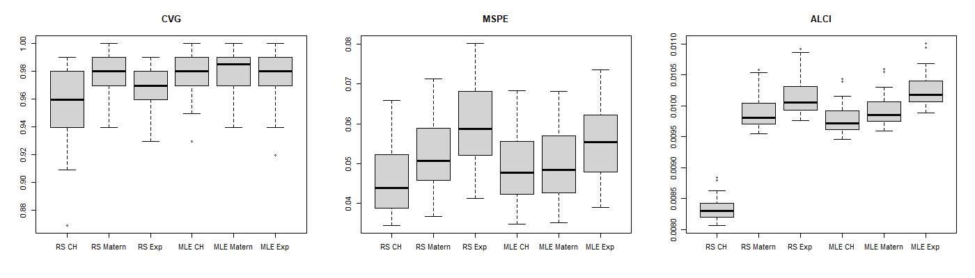
Figure 1: (Left to right). Boxplots of coverage of 95% confidence intervals (CVG), mean squared prediction error (MSPE) and average length of the confidence intervals (ALCI). Results are for CH, Matérn and squared Exponential (Exp) covariances, with parameters set via rescaling (RS) or MLE. Boxplots are computed over 30 randomly chosen training and testing data sets. Here $d=1$ and the true function $f(x)$ is a realization of Brownian motion.

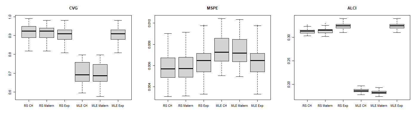
Figure 2: (Left to right). Boxplots of coverage of 95% confidence intervals (CVG), mean squared prediction error (MSPE) and average length of the confidence intervals (ALCI). Results are for CH, Matérn and squared Exponential (Exp) covariances, with parameters set via rescaling (RS) or MLE. Boxplots are computed over 30 randomly chosen training and testing data sets. Here $d=1$, and the true function $f(x)$ is a realization of stationary Gaussian process with mean $0$ and covariance function $M(h;1,1,1)$.

5.2 The Case of $d=2$

In the $d=2$ case, we simulate on $n=1600$ data points uniformly drawn from $[0,1]^{2}$ and select 160 data points uniformly as the testing data, the rest as training data. For this set, parameters of interest are obtained by MLE and rescaled methods. We repeat the procedure on 30 randomly picked testing and training data sets.

We let the true function $f(x)$ be a realization of stationary Gaussian process with mean 0 and covariance function $M(h;1,1,1)$. This true function is differentiable but not in Sobolev space $H^{2}([0,1]^{2})$. From Figure 3, the three rescaled priors have same behavior as in $d=1$ case, outperforming MLE in terms of empirical coverage of the confidence intervals.

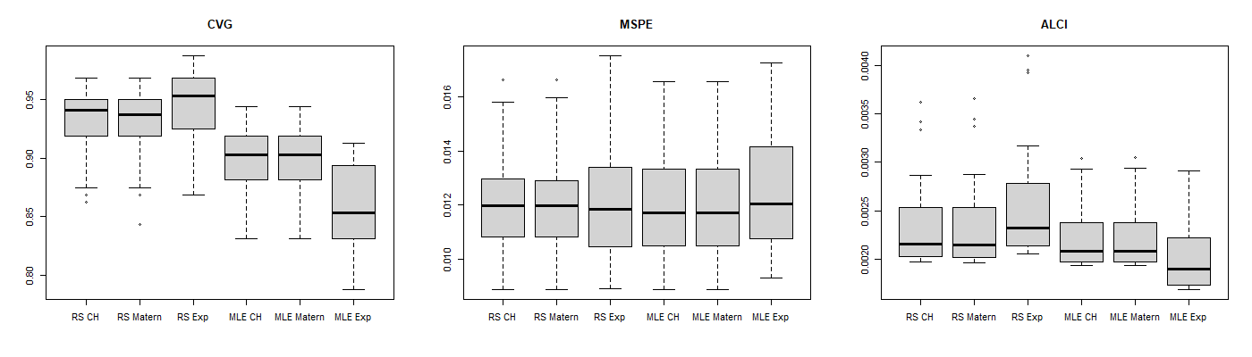
Figure 3: (Left to right). Boxplots of coverage of 95% confidence intervals (CVG), mean squared prediction error (MSPE) and average length of the confidence intervals (ALCI). Results are for CH, Matérn and squared Exponential (Exp) covariances, with parameters set via rescaling (RS) or MLE. Boxplots are computed over 30 randomly chosen training and testing data sets. Here $d=2$, and the true function $f(x)$ is a realization of stationary Gaussian process with mean 0 and covariance function $M(h;1,1,1)$.

6 Results on Atmospheric NO₂ data

In this section we study the relationship between location and the level of Nitrogen Dioxide (NO₂), a known environmental pollutant, with the nonparametric normal regression model described in Section 2.4. Our data are the level of NO₂ concentration, measured in parts per million (ppm), the city of York, UK from December, 2022. We aim to predict the level of NO₂ by location information $(X,Y)$ = (latitude, longitude). To evaluate the performance, we randomly select 65 data points as the validation set and the rest 154 data points as the training set. The training and validation data sets are displayed in Figure 4. We select parameters based on the training set, and then evaluate the prediction performance of our nonparametric normal regression model with rescaled CH, Matérn and squared exponential priors on the testing set.

In our theoretical results, the smoothness parameter $\nu$ should be greater than the regularity of the true function. Therefore, here we set $\nu=5$ for CH and Matérn covariances as a sufficiently large $\nu$. Then, we use maximum likelihood method to estimate the parameters in CH, Matérn and squared exponential covariance functions. We set those estimated parameter as initial value and we rescale $\beta$, $\phi$, $c$ to achieve optimal prediction performance. To avoid singularity in matrix calculation, we center and scale $X$ with $100(X-\bar{X})$ and $Y$ with $100(Y-\bar{Y})$. We also rescale NO₂ by dividing it by the sample maximum. The results are repeated over 30 random splits of the data set, into training and testing sets of the same size. We summarize the results in Figure 5. From the boxplots, we observe CVG, MSE and ALCI of rescaled CH, Matérn, squared exponential coavarinces are better than their corresponding MLE-based counterparts. Within these rescaled priors, CH is slightly better than squared exponential, while Matérn has the worst performance.

Figure 6 displays the scatterplots of residuals versus predicted values under rescaled CH, Matérn and squared exponential methods on the validation set, along with the posterior predivctive intervals. Out of the 65 validation data points, 58 of the validation data points lie inside the 95% predictive intervals for the rescaled CH method. These numbers are respectively 57 and 56 for the rescaled Matérn and squared exponential methods, indicating similar coverage. However, the 95% predictive intervals from the rescaled CH method are much shorter in general compared to rescaled Matérn or squared exponential. Overall, rescaled CH performs the best, with rescaled Matérn and rescaled squared exponential performing similarly, and both performing worse than CH.

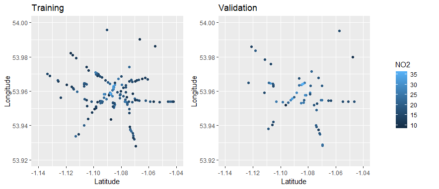
Figure 4: Scatter plot of NO₂ measurements in York, UK in December 2022.

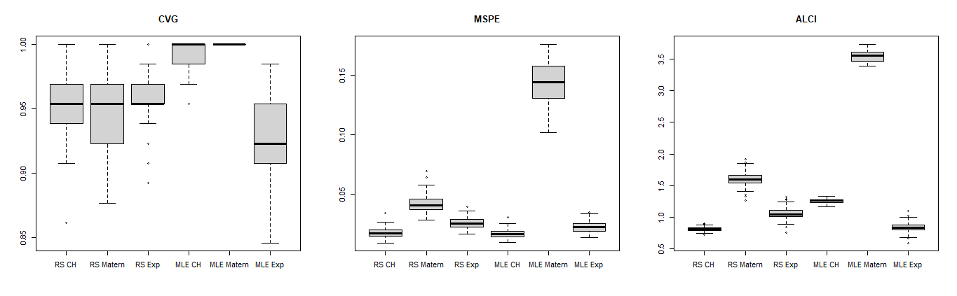
Figure 5: (Left to right). Boxplots of coverage of 95% confidence intervals (CVG), mean squared prediction error (MSPE) and average length of the confidence intervals (ALCI). Results are for CH, Matérn and squared Exponential (Exp) covariances, with parameters set via rescaling (RS) or MLE, for the NO₂ data.

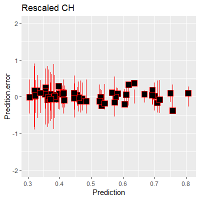
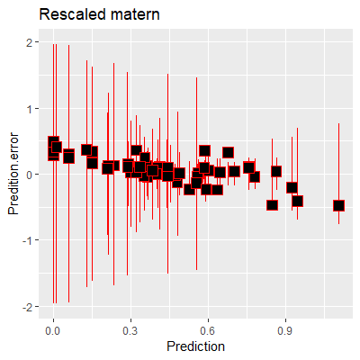
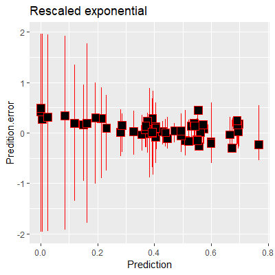
Figure 6: Prediction error vs. residuals for the NO₂ data validation set for CH, Matérn and squared exponential covariances under rescaling. Bars indicate posterior predictive 95% intervals.

7 Discussion

This paper studies posterior concentration properties of nonparametric normal regression with fixed design. For $\eta$-regular functions, we find by rescaling the parameters in Matérn class, we can improve the classical posterior contraction rate result in van der Vaart and van Zanten, (2007) to optimal minimax rate. We also study the CH prior, and show it also attains the optimal minimax rate for $\eta$-regular functions under rescaling. Although we demonstrate the optimal minimax rates, there are still areas of further investigations.

We obtain the optimal minimax posterior contraction rate by rescaling. However, the choice of the rescaling parameter depends on the smoothness of the function of interest ($\eta$ in our case), which is always unknown in practice. It is natural to choose the lengthscale using the data. Szabó et al., (2013) applies an empirical Bayes method and obtains the rescaling parameter by maximizing the marginal Bayesian likelihood. However, the theoretical properties of this procedure are known only for the Gaussian white noise model. van der Vaart and van Zanten, (2009) consider a fully Bayesian alternative by putting a hyperprior on the rescaling parameter for the squared exponential process prior. Following our work, for Matérn and CH covariances, one can also put inverse gamma prior on the rescaling parameter. The posterior contraction rates of these models remain to be explored. Moreover, using an inverse gamma prior on the scale parameter $\phi$ of the Matérn class is quite similar to the way the CH covariance function as a mixture of the Matérn class, and it is interesting to investigate its implication on posterior contraction rates.

In our paper, we restricted our interest to nonparametric normal regression with fixed design. For the random design case, one assumes that given the function $f:[0,1]^{d}\rightarrow\mathbb{R}$ on the $d$-dimensional unit cube $[0,1]^{d}$, the data $\left(X_{1},Y_{1}\right),\ldots,\left(X_{n},Y_{n}\right)$ are independent, $X_{i}$ having a density $g$ on $[0,1]^{d}$, and $Y_{j}$s are generated according to $Y_{j}=f\left(X_{j}\right)+\varepsilon_{j}$, errors $\varepsilon_{j}\sim N\left(0,\sigma^{2}\right)$ are independent given $X_{j}$. van der Vaart and van Zanten, (2011); Pati et al., (2015); Jiang and Tokdar, (2021) obtain posterior contraction rate for random design case, and their works show the key to get (nearly) optimal rate is to define a proper discrepancy measure. In a future work, one may attempt to construct the discrepancy measure under which rescaled Matérn and CH process priors attain the optimal minimax rates under random design.

Appendix

.1 Proofs of Main Results

Proof of Lemma 3.2.

The small ball exponent can be obtained from the metric entropy (logarithm of the $\epsilon$-covering number) of unit ball $\mathbb{H}_{1}$ of the RKHS of the Gaussian process $W$ (Li and Linde,, 1999). The transform $\mathcal{F}_{\phi}\psi$ of $\psi$ given in (9) is, up to constants, the function $g=\psi\cdot{m_{M}^{\phi}}$, and for the minimal choice of $\psi$ as in (11), for Matérn covariance we have:

$$\|\mathcal{F}_{\phi}\psi\|_{\mathbb{H}^{\phi}}^{2}=\int|g(\lambda)|^{2}\left({m_{M}^{\phi}}(\lambda)\right)^{-1}d\lambda\\ =\int|g(\lambda)|^{2}(1+\lambda^{2})^{(v+d/2)}\frac{(1+\lambda^{2})^{-(v+d/2)}}{m_{M}^{\phi}(\lambda)}d\lambda.$$

Since $\frac{(1+\lambda^{2})^{-(v+d/2)}}{m_{M}^{\phi}(\lambda)}\gtrsim\phi^{2v}$, we have $\|\mathcal{F}_{\phi}\psi\|_{\mathbb{H}^{\phi}}^{2}\geq C\phi^{2v}\|g\|^{2}_{2,2,v+d/2}$, and thus the unit ball of the RKHS is contained in the Sobolev ball with radius $\phi^{-v}$ (up to a constant) of order $v+d/2$. By Proposition C.7 of Ghosal and van der Vaart, (2017), the metric entropy of such a Sobolev ball is bounded above by a constant times $(\phi^{-v})^{\frac{d}{v+d/2}}\varepsilon^{-\frac{d}{v+d/2}}$. Next, by Theorem 1.2 of Li and Linde, (1999) ,

$$\varphi_{0}(\varepsilon)\lesssim\varepsilon^{-\frac{2\frac{d}{v+d/2}}{2-\frac{d}{v+d/2}}}\left[(\phi^{-v})^{\frac{d}{v+d/2}}\right]^{\frac{2v+d}{2v}}=\varepsilon^{-d/v}\phi^{-d}.$$ (13)

From the proof of Proposition 3.1 of Li and Linde, (1999), this bound holds for all $\varepsilon>0$ satisfying:

$$\phi^{\frac{vd}{v+d/2}}\lesssim(\varphi_{0}(\varepsilon/2))^{\frac{d}{2(v+d/2)}}\varepsilon^{-\frac{d}{v+d/2}}.$$

By assumption we also have $\phi<1$. Thus,

$$\varphi_{0}(\varepsilon/2)=-\log P\left(\sup_{t\in[0,1]^{d}}|W_{t}^{\phi}|\leq\varepsilon/2\right)\geq-\log P\left(\sup_{t\in[0,1]^{d}}|W_{t}|\leq\varepsilon/2\right),$$

where the last inequality follows directly form the definition of the rescaled process. (13) holds for all $\varepsilon$ in an interval independent of $\phi$ since the right hand side is independent of $\phi$ , completing the proof. ∎

Proof of Lemma 3.3.

Let $\zeta$, $\zeta_{\phi}$, $h$ be the same construction as in the proof of Lemma 11.37 in Ghosal and van der Vaart, (2017). Let $\kappa:\mathbb{R}\rightarrow\mathbb{R}$ be a function with a real, symmetric Fourier transform $\hat{\kappa}(\lambda)=(2\pi)^{-1}\int e^{i\lambda t}\kappa(t)dt$, then $\hat{\kappa}$ equals $1/(2\pi)$ in a neighborhood of 0 which has compact support, with $\int\kappa(t)dt=1$ and $\int(it)^{k}\kappa(t)dt=0$ for $k\geq 1$. For $t=\left(t_{1},\ldots,t_{d}\right)$, define $\zeta(t)=\prod_{i=1}^{d}\kappa\left(t_{i}\right)$. Then $\zeta(t)$ integrates to 1, has finite absolute moments of all orders, and vanishing moments of all orders bigger than 0.

For $\phi>0$, set $\zeta_{\phi}(x)=\phi^{-d}\zeta(x/\phi)$ and $h=\zeta_{\phi^{\theta}}*w_{0}$, where $\theta\geq 1$ is to be determined. By slimilar arguments in van der Vaart and van Zanten, (2009), it follows that $\left\|w_{0}-\zeta_{\phi^{\theta}}*w_{0}\right\|_{\infty}\leq C_{w_{0}}\phi^{\eta\theta}$ and $C_{w_{0}}$ only depends on $w_{0}$. We assume that the support of $\hat{\zeta}(\lambda)$ is in the set $\{\lambda:\|\lambda\|\leq M\}$. The Fourier transform of $h$ is $\hat{h}(\lambda)=\hat{\zeta}(\phi^{\theta}\lambda)\hat{w_{0}}(\lambda)$. Then $h=2\pi\int e^{-it\lambda}\hat{\zeta}(\phi^{\theta}\lambda)\hat{w_{0}}(\lambda)d\lambda=2\pi\mathcal{F}_{\phi}\left(\frac{\hat{\zeta}(\phi^{\theta}\lambda)\hat{w_{0}}(\lambda)}{m_{M}^{\phi}(\lambda)}\right)$. By (11) we have:

$$\begin{split}\|h\|_{\mathbb{H}^{\phi}}^{2}&=\left\|2\pi\mathcal{F}_{\phi}\left(\frac{\hat{\zeta}(\phi^{\theta}\lambda)\hat{w_{0}}(\lambda)}{m_{M}^{\phi}(\lambda)}\right)\right\|_{\mathbb{H}^{\phi}}^{2}\\ &\leq(2\pi)^{2}\int|\hat{\zeta}(\phi^{\theta}\lambda)\hat{w_{0}}(\lambda)|^{2}\frac{1}{m^{\phi}_{M}(\lambda)}d\lambda\\ &\leq\tilde{D}_{w_{0}}\cdot\sup_{\lambda}\left[(1+{\|\lambda\|^{2}})^{-\eta}\left(m^{\phi}_{M}(\lambda)\right)^{-1}|\hat{\zeta}(\phi^{\theta}\lambda)|^{2}\right]\times\|w_{0}\|^{2}_{2,2,\eta}\\ &=\tilde{D}_{w_{0}}\cdot\sup_{\|\lambda\|\leq M/\phi^{\theta}}\left[(1+{\|\lambda\|^{2}})^{-\eta}\left(m^{\phi}_{M}(\lambda)\right)^{-1}|\hat{\zeta}(\phi^{\theta}\lambda)|^{2}\right]\times\|w_{0}\|^{2}_{2,2,\eta}\\ &\leq D_{w_{0}}\cdot\sup_{\|\lambda\|\leq M/\phi^{\theta}}\left[(1+{\|\lambda\|^{2}})^{-\eta}\left(m^{\phi}_{M}(\lambda)\right)^{-1}\right]\times\|w_{0}\|^{2}_{2,2,\eta}\\ &=D_{w_{0}}\cdot\max_{\|\lambda\|=0,M/\phi^{\theta}}\left[(1+{\|\lambda\|^{2}})^{-\eta}\left(m^{\phi}_{M}(\lambda)\right)^{-1}\right]\times\|w_{0}\|^{2}_{2,2,\eta}\\ &=D_{w_{0}}\cdot\max\left\{\phi^{-d},\phi^{2v-2\theta(v+d/2-\eta)}\right\}\times\|w_{0}\|^{2}_{2,2,\eta},\end{split}$$ (14)

where $\tilde{D}_{w_{0}}$, $D_{w_{0}}$ only depend on $w_{0}$, and the second last equality is due to the fact that $\log[(1+{\|\lambda\|^{2}})^{-\eta}\left(m^{\phi}_{M}(\lambda)\right)^{-1}]$ attains its maximum at the boundary, i.e., $\|\lambda\|=0$ or $M/\phi^{\theta}$(by taking derivative with respect to $\|\lambda\|^{2}$ ). When $\theta>\frac{2v+d}{2v+d-2\eta}$, we have $\|h\|_{\mathbb{H}^{\phi}}^{2}\lesssim\phi^{2v-2\theta(v+d/2-\eta)}$. ∎

Proof of Theorem 3.5.

For the rescaled Matérn class, when $\|\lambda\|\geq\phi^{-1}$, its spectral density satisfies

$$m^{\phi}_{M}(\lambda)\geq c_{0}\phi^{-2v}\|\lambda\|^{-(2v+d)},$$

where $c_{0}$ does not depend on $\phi$. By the corollary in Lifshits and Tsirelson, (1987), we have:

$$P\left(\sup_{t\in[0,1]^{d}}|W_{t}^{\phi}|\leq\varepsilon\right)\leq\exp(-C\phi^{-d}\varepsilon^{-d/v}),$$

where $C$ is a constant that only depends on $v$ and $d$. Thus, we have $\varphi_{0}(\varepsilon)\gtrsim\phi^{-d}\varepsilon^{-d/v}$. The second part of this theorem can be obtain by applying Theorem 11.23 of Ghosal and van der Vaart, (2017), since $\epsilon_{n}=\max\left\{\left({\phi^{2v}}/{n}\right)^{\frac{\eta}{2v+d}},\left({\phi^{-d}}/{n}\right)^{\frac{v}{2v+d}}\right\}$ satisfies the rate equation $\varphi_{w_{0}}(\epsilon_{n})\leq n\epsilon_{n}^{2}$ (by the statement before Theorem 3.4). Thus, $\varphi_{w_{0}}(\delta_{n})\geq C_{0}n\epsilon_{n}^{2}$ for sufficiently large constant $C_{0}$ if $\delta_{n}\geq 1$ and $\phi^{-d}\gtrsim n$. ∎

Proof of Lemma 3.6.

Let $g=\psi m$, and for the minimal choice of $\psi$ as in (12), we have for the CH covariance:

$$\|\mathcal{F}_{(\alpha,\beta)}\psi\|_{\mathbb{H}^{\alpha,\beta}}^{2}=\int|g(\lambda)|^{2}(m_{CH}^{\alpha,\beta})^{-1}(\lambda)d\lambda\\ =\int|g(\lambda)|^{2}(1+\lambda^{2})^{(v+d/2)}\frac{(1+\lambda^{2})^{-(v+d/2)}}{m_{CH}^{\alpha,\beta}(\lambda)}d\lambda.$$

By Lemma .3, we have $\frac{(1+\lambda^{2})^{-(v+d/2)}}{m_{CH}^{\alpha,\beta}(\lambda)}\gtrsim\frac{\Gamma(\alpha)\beta^{2v}}{\Gamma(\alpha+v)}$, then $\|\mathcal{F}_{(\alpha,\beta)}\psi\|_{\mathbb{H}^{\alpha,\beta}}^{2}\geq C\frac{\Gamma(\alpha)\beta^{2v}}{\Gamma(\alpha+v)}\|g\|^{2}_{2,2,v+d/2}$, and the unit ball of RKHS is contained in the Sobolev ball of radius $\sqrt{\frac{\Gamma(\alpha+v)}{\Gamma(\alpha)\beta^{2v}}}$ (up to a constant) of order $v+d/2$. By Proposition C.7 in Ghosal and van der Vaart, (2017), the metric entropy of such a Sobolev ball is bounded by a constant times $(\frac{\Gamma(\alpha+v)}{\Gamma(\alpha)\beta^{2v}})^{\frac{d/2}{v+d/2}}\varepsilon^{-\frac{d}{v+d/2}}$. By Theorem 1.2 of Li and Linde, (1999) ,

$$\begin{split}\varphi_{0}(\varepsilon)&\lesssim\varepsilon^{-\frac{2\frac{d}{v+d/2}}{2-\frac{d}{v+d/2}}}\left[\left(\frac{\Gamma(\alpha+v)}{\Gamma(\alpha)\beta^{2v}}\right)^{\frac{d/2}{v+d/2}}\right]^{\frac{2v+d}{2v}}=\varepsilon^{-d/v}\left(\frac{\Gamma(\alpha+v)}{\Gamma(\alpha)\beta^{2v}}\right)^{d/(2v)}.\end{split}$$ (15)

From the proof of Proposition 3.1 of Li and Linde, (1999), this bound holds for all $\varepsilon>0$ satisfying,

$$\left[\frac{\Gamma(\alpha)\beta^{2v}}{\Gamma(\alpha+v)}\right]^{\frac{d/2}{v+d/2}}\lesssim(\varphi_{0}(\varepsilon/2))^{\frac{d}{2(v+d/2)}}\varepsilon^{-\frac{d}{v+d/2}}.$$

Similar to the proof in Theorem 3.5, by Lemma .4, for rescaled CH class, when $\|\lambda\|\geq(\alpha+v-1)\beta^{-1}$, its spectral density satisfies:

$$m^{\alpha,\beta}_{CH}(\lambda)\gtrsim\frac{\Gamma(\alpha+v)}{\Gamma(\alpha)\beta^{2v}}\|\lambda\|^{2v+d},$$

and we have:

$$P\left(\sup_{t\in[0,1]^{d}}|W_{t}^{\alpha,\beta}|\leq\varepsilon/2\right)\leq\exp\left(-C\left(\frac{\Gamma(\alpha+v)}{\Gamma(\alpha)\beta^{2v}}\right)^{d/(2v)}\varepsilon^{-d/v}\right),$$

where $\varepsilon$ and $C$ only depend on $v$ and $d$. When $\frac{\Gamma(\alpha+v)}{\Gamma(\alpha)\beta^{2v}}>1$, we have,

$$\varphi_{0}(\varepsilon/2)=-\log P\left(\sup_{t\in[0,1]^{d}}|W_{t}^{\alpha,\beta}|\leq\varepsilon/2\right)\geq C\left(\frac{\Gamma(\alpha+v)}{\Gamma(\alpha)\beta^{2v}}\right)^{d/(2v)}\varepsilon^{-d/v}\geq C\varepsilon^{-d/v}.$$

Since the right hand side is independent of $\alpha,\beta$, it follows that (15) holds for all $\varepsilon$ in an interval independent of $\alpha,\beta$. ∎

Proof of Lemma 3.7.

Here, we use the exact construction in the proof of Lemma 3.3, but let $h=\zeta_{\beta^{\theta}}*w_{0}$, $\theta>1$. By Lemma .4, when $\theta>\frac{v+d/2}{v+d/2-\eta}$, $\beta^{-1}\gtrsim\ln n$ and $\alpha\lesssim\sqrt{\ln\ln n}$, we have

$$\begin{split}\|h\|_{\mathbb{H^{\alpha,\beta}}}^{2}&=\left\|2\pi\mathcal{F}_{(\alpha,\beta)}\left(\frac{\hat{\zeta}(\beta^{\theta}\lambda)\hat{w_{0}}(\lambda)}{m_{CH}^{\alpha,\beta}(\lambda)}\right)\right\|_{\mathbb{H^{\alpha,\beta}}}^{2}\\ &\leq\tilde{D}_{w_{0}}\cdot\int|\hat{\varphi}(\beta^{\theta}\lambda)\hat{w_{0}}(\lambda)|^{2}\frac{1}{{m_{CH}^{\alpha,\beta}}(\lambda)}d\lambda\\ &\leq\tilde{D}_{w_{0}}\cdot\sup_{\lambda}[(1+{\|\lambda\|^{2}})^{-\eta}({m_{CH}^{\alpha,\beta}})^{-1}(\lambda)|\hat{\varphi}(\beta^{\theta}\lambda)|^{2}]\times\|w_{0}\|^{2}_{2,2,\eta}\\ &=\tilde{D}_{w_{0}}\cdot\sup_{\|\lambda\|\leq M/\beta^{\theta}}[(1+{\|\lambda\|^{2}})^{-\eta}({m_{CH}^{\alpha,\beta}})^{-1}(\lambda)|\hat{\varphi}(\beta^{\theta}\lambda)|^{2}]\times\|w_{0}\|^{2}_{2,2,\eta}\\ &\leq{D}_{w_{0}}\cdot\sup_{\|\lambda\|\leq M/\beta^{\theta}}[(1+{\|\lambda\|^{2}})^{-\eta}({m_{CH}^{\alpha,\beta}})^{-1}(\lambda)]\times\|w_{0}\|^{2}_{2,2,\eta}\\ &\lesssim\max\left\{\frac{\Gamma(\alpha)}{\Gamma(\alpha-d/2)\beta^{d}},\frac{\Gamma(\alpha)e^{\alpha}}{\beta^{-2v}\Gamma(\alpha-d/2)\alpha}\left(\frac{\alpha+v-1}{\beta^{2}}\right)^{v+d/2-\eta},\right.\\ &\left.\qquad(\beta^{2\theta})^{-v-d/2+\eta}\frac{\Gamma(\alpha)\beta^{2v}}{\Gamma(\alpha+v)}\right\}\\ &\leq(\beta^{2\theta})^{-v-d/2+\eta}\frac{\Gamma(\alpha)\beta^{2v}}{\Gamma(\alpha+v)},\end{split}$$ (16)

where $\tilde{D}_{w_{0}}$ and ${D}_{w_{0}}$ depend only on $w_{0}$. ∎

Proof of Theorem 3.9.

For the rescaled CH class, by Lemma .4, when $\|\lambda\|\geq(\alpha+v-1)\beta^{-1}$, its spectral density satisfies:

$$m^{\alpha,\beta}_{CH}(\lambda)\geq c_{0}\beta^{-2v}\|\lambda\|^{-(2v+d)},$$

where $c_{0}$ does not depend on $\alpha,\beta$. Then following the same steps in the proof of Theorem 3.5, completes the present proof. ∎

Proof of Theorem 4.1.

There exists constant $C>0$ such that

$$1/C\cdot m_{M}^{\bm{\lambda_{\max}}}(\bm{h})\leq m_{M}^{\bm{B}}(\bm{h})\leq Cm_{M}^{\bm{\lambda_{\max}}}(\bm{h}),$$

and,

$$1/C\cdot m^{\alpha,\lambda_{\max}}_{CH}(\bm{h})\leq m^{\alpha,\bm{B}}_{CH}(\bm{h})\leq Cm^{\alpha,\lambda_{\max}}_{CH}(\bm{h}).$$

Then the proof of this theorem follows similarly to the proofs of Theorem 3.4 and Theorem 3.8. ∎

.2 Ancillary Results

Posterior contraction rate of stationary Gaussian processes is partly determined by the tail behavior of its spectral density. In this subsection, we establish some ancillary results and some useful properties of the spectral density of the CH covariance function, needed in the proofs of the main theorems.

Let $\Gamma(x),\;x\in\mathbb{R}^{+}$ denote the gamma function for a positive real-valued argument. The lower and upper incomplete gamma functions are defined respectively as:

$$\gamma(a,x)=\int_{0}^{x}e^{-t}t^{a-1}dt;\qquad\Gamma(a,x)=\int_{x}^{\infty}e^{-t}t^{a-1}dt,\qquad a>0.$$

A useful inequality (Alzer,, 1997; Gautschi,, 1998) for the incomplete gamma function is:

$$\quad\left(1-e^{-s_{a}x}\right)^{a}<\frac{\gamma(a,x)}{\Gamma(a)}<\left(1-e^{-r_{a}x}\right)^{a},\quad 0\leq x<\infty,\quad a>0,\quad a\neq 1,$$ (17)

where,

$$r_{a}=\left\{\begin{array}[]{ll}{[\Gamma(1+a)]^{-1/a}}&\text{ if }0<a<1,\\ 1&\text{ if }a>1,\end{array}\quad s_{a}=\begin{cases}1&\text{ if }0<a<1,\\ {[\Gamma(1+a)]^{-1/a}}&\text{ if }a>1.\end{cases}\right.$$

Lemma .1.

We have,

$$\lim_{x\to\infty}\frac{\gamma(x+1,x)}{\Gamma(x+1)}=1/2.$$ (18)

Proof of Lemma .1.

(At the time of writing, a sketch of the proof is available at: https://math.stackexchange.com/questions/3751528/limits-of-the-incomplete-gamma-function, which we reproduce below, unable to locate a persistent citable academic item.) Let $t=x+u\sqrt{x}$. Then,

$$\Gamma(x+1,x) =\int_{x}^{\infty}t^{x}e^{-t}\mathrm{~{}d}t=x^{x+\frac{1}{2}}e^{-x}\int_{0}^{\infty}\left(1+\frac{u}{\sqrt{x}}\right)^{x}e^{-\sqrt{x}u}\mathrm{~{}d}u.$$ (19)

Next, note that:

$$\lim_{x\rightarrow\infty}\left(1+\frac{u}{\sqrt{x}}\right)^{x}e^{-\sqrt{x}u}=e^{-\frac{u^{2}}{2}}.$$

Applying the inequality $\log(1+x)\leq x-\frac{x^{2}}{2(x+1)}$ for $x\geq 0$ shows that,

$$\left(1+\frac{u}{\sqrt{x}}\right)^{x}e^{-\sqrt{x}u}\leq e^{-\frac{u^{2}}{2(u+1)}},$$

for all $x\geq 1$ and $u\geq 0$. Since this bound is integrable on $[0,\infty)$, by the dominated convergence theorem,

$$\lim_{x\rightarrow\infty}\int_{0}^{\infty}\left(1+\frac{u}{\sqrt{x}}\right)^{x}e^{-\sqrt{x}u}\mathrm{~{}d}u =\int_{0}^{\infty}e^{-\frac{u^{2}}{2}}\mathrm{~{}d}u=\sqrt{\frac{\pi}{2}}.$$ (20)

An application of Stirling’s formula yields:

$$\Gamma(x+1) \sim\sqrt{2\pi}x^{x+\frac{1}{2}}e^{-x},\quad\text{ as }\quad x\rightarrow\infty.$$ (21)

Combining (19), (20) and (21), we obtain,

$$\lim_{x\rightarrow\infty}\frac{\Gamma(x+1,x)}{\Gamma(x+1)}=\frac{1}{2}.$$

Noting that $\gamma(x+1,x)+\Gamma(x+1,x)=\Gamma(x+1)$ completes the proof. ∎

Lemma .2.

Let $\{a_{n}\},\{b_{n}\}>0$ be sequences such that $a_{n}=O(1)$. Then, we have, as $n\to\infty$,

$$\int_{0}^{a_{n}}x^{b_{n}-1}\exp(-x)dx\asymp a_{n}^{b_{n}}/b_{n}.$$

Proof of Lemma .2.

For the upper bound, we have,

$$\int_{0}^{a_{n}}x^{b_{n}-1}\exp(-x)dx\leq\int_{0}^{a_{n}}x^{b_{n}-1}dx=a_{n}^{b_{n}}/b_{n}.$$

For the lower bound,

$$\int_{0}^{a_{n}}x^{b_{n}-1}\exp(-x)dx\geq\exp(-a_{n})\int_{0}^{a_{n}}x^{b_{n}-1}dx=\exp(-a_{n})\cdot{a_{n}}^{b_{n}}/{b_{n}}\gtrsim{a_{n}}^{b_{n}}/{b_{n}}.\qed$$

The next lemma obtains the upper and lower bounds for the spectral density of the CH class.

Lemma .3.

If $\alpha>d/2+1$ and $\beta^{2}=O(1)$ as $n\to\infty$, then,

$$\frac{\Gamma(\alpha-d/2)}{\Gamma(\alpha)}\beta^{d}\lesssim(1+\lambda^{2})^{(v+d/2)}m^{\alpha,\beta}_{CH}(\lambda)\lesssim\frac{\Gamma(\alpha+v)}{\Gamma(\alpha)\beta^{2v}}.$$

Proof of Lemma .3.

Let $h=\beta^{2}/(2\phi^{2})$. Then,

$$\begin{split}&(1+\lambda^{2})^{(v+d/2)}m^{\alpha,\beta}_{CH}(\lambda)\\ =&\frac{\sigma^{2}2^{v-\alpha}v^{v}\beta^{2\alpha}}{\pi^{d/2}\Gamma(\alpha)}(1+\lambda^{2})^{(v+d/2)}\int_{0}^{\infty}(2v\phi^{-2}+\lambda^{2})^{-v-d/2}\phi^{-2(v+\alpha+1)}\exp{(-\beta^{2}/(2\phi^{2}))d\phi^{2}}\\ =&\frac{\sigma^{2}2^{v-\alpha}v^{v}\beta^{2\alpha}}{\pi^{d/2}\Gamma(\alpha)}\left[\int_{0}^{1}\left(\frac{1+\lambda^{2}}{2v+\phi^{2}\lambda^{2}}\right)^{(v+d/2)}\phi^{-2(-d/2+\alpha+1)}\exp{(-\beta^{2}/(2\phi^{2}))}d\phi^{2}\right.\\ &+\left.\int_{1}^{\infty}\left(\frac{1+\lambda^{2}}{2v\phi^{-2}+\lambda^{2}}\right)^{(v+d/2)}\phi^{-2(v+\alpha+1)}\exp{(-\beta^{2}/(2\phi^{2}))}d\phi^{2}\right]\\ \gtrsim&\frac{\sigma^{2}2^{v-\alpha}v^{v}\beta^{2\alpha}}{\pi^{d/2}\Gamma(\alpha)}\left[\left(\frac{\beta^{2}}{2}\right)^{d/2-\alpha}\int_{\frac{\beta^{2}}{2}}^{\infty}h^{\alpha-d/2-1}\exp(-h)dh+\left(\frac{\beta^{2}}{2}\right)^{-v-\alpha}\int^{\frac{\beta^{2}}{2}}_{0}h^{\alpha+v-1}\exp(-h)dh\right]\\ \gtrsim&\frac{1}{\Gamma(\alpha)}\left[\left(\frac{\beta^{2}}{2}\right)^{d/2}\int_{\frac{\beta^{2}}{2}}^{\infty}h^{\alpha-d/2-1}\exp(-h)dh+\left(\frac{\beta^{2}}{2}\right)^{-v}\int^{\frac{\beta^{2}}{2}}_{0}h^{\alpha+v-1}\exp(-h)dh\right].\end{split}$$

By Lemma .2 and Stirling’s approximation, we have $\int^{{\beta^{2}}/{2}}_{0}h^{\alpha+v-1}\exp(-h)dh\asymp\frac{({\beta^{2}}/{2})^{\alpha+v}}{\alpha+v},$ and, $\int_{{\beta^{2}}/{2}}^{\infty}h^{\alpha-d/2-1}\exp(-h)dh\asymp\Gamma(\alpha-d/2),$ yielding the lower bound. The upper bound follows similarly. ∎

The next lemma gives an alternative lower bound for the spectral density of CH class, depending on the relationship between $\alpha$ and $\beta$.

Lemma .4.

Suppose $\beta^{2}=O(1)$ and $\alpha>d/2+1$, for $\alpha$ fixed or tending to infinity as $n\to\infty$. Then,

$$(1+\lambda^{2})^{v+d/2}m^{\alpha,\beta}_{CH}(\lambda)\gtrsim\left\{\begin{array}[]{lll}\frac{\Gamma(\alpha-d/2)\beta^{d}}{\Gamma(\alpha)}(1+\lambda^{2})^{v+d/2},&\text{ if }\lambda^{2}\beta^{2}\leq 1,\\ \frac{\beta^{-2v}\Gamma(\alpha-d/2)}{\Gamma(\alpha)}\frac{\alpha}{e^{\alpha}},&\text{ if }1<\lambda^{2}\beta^{2}<\alpha+v-1,\\ \frac{\beta^{-2v}\Gamma(\alpha+v)}{\Gamma(\alpha)},&\text{ if }\lambda^{2}\beta^{2}\geq\alpha+v-1.\end{array}\right.$$

Proof of Lemma .4.

We only prove the $\alpha\to\infty$ case. The fixed $\alpha$ case can be proved by the same method. Let $h=\beta^{2}/(2\phi^{2})$. Then,

$$\begin{split}&(1+\lambda^{2})^{(v+d/2)}m^{\alpha,\beta}_{CH}(\lambda)\\ =&\frac{\sigma^{2}2^{v-\alpha}v^{v}\beta^{2\alpha}}{\pi^{d/2}\Gamma(\alpha)}\int_{0}^{\infty}\left(\frac{1+\lambda^{2}}{2v\phi^{-2}+\lambda^{2}}\right)^{v+d/2}\phi^{-2(v+\alpha+1)}\exp{(-\beta^{2}/(2\phi^{2}))d\phi^{2}}\\ =&\frac{\sigma^{2}{(4v)}^{v}\beta^{-2v}}{\pi^{d/2}\Gamma(\alpha)}\int_{0}^{\infty}\left(\frac{1+\lambda^{2}}{4vh\beta^{-2}+\lambda^{2}}\right)^{v+d/2}h^{v+\alpha-1}\exp(-h)dh\\ =&\frac{\sigma^{2}{(4v)}^{v}\beta^{-2v}}{\pi^{d/2}\Gamma(\alpha)}\left[\int_{0}^{\lambda^{2}\beta^{2}}\left(\frac{1+\lambda^{2}}{4vh\beta^{-2}+\lambda^{2}}\right)^{v+d/2}h^{v+\alpha-1}\exp(-h)dh\right.\\ &+\left.\int_{\lambda^{2}\beta^{2}}^{\infty}\left(\frac{1+\lambda^{2}}{4vh\beta^{-2}+\lambda^{2}}\right)^{v+d/2}h^{v+\alpha-1}\exp(-h)dh\right]\\ \asymp&\frac{\beta^{-2v}}{\Gamma(\alpha)}\left[\int_{0}^{\lambda^{2}\beta^{2}}\left(\frac{1+\lambda^{2}}{4vh\beta^{-2}+\lambda^{2}}\right)^{v+d/2}h^{v+\alpha-1}\exp(-h)dh\right.\\ &+\left.[(1+\lambda^{2})\beta^{2}]^{v+d/2}\int_{\lambda^{2}\beta^{2}}^{\infty}h^{\alpha-d/2-1}\exp(-h)dh\right].\end{split}$$ (22)

When $\lambda^{2}\beta^{2}\leq 1$, by Lemma .2:

$$\begin{split}&(1+\lambda^{2})^{(v+d/2)}m^{\alpha,\beta}_{CH}(\lambda)\\ &\gtrsim\frac{\beta^{-2v}}{\Gamma(\alpha)}[(1+\lambda^{2})\beta^{2}]^{v+d/2}\int_{\lambda^{2}\beta^{2}}^{\infty}h^{\alpha-d/2-1}\exp(-h)dh\\ &\asymp\frac{\beta^{-2v}}{\Gamma(\alpha)}[(1+\lambda^{2})\beta^{2}]^{v+d/2}\Gamma(\alpha-d/2)\\ &\asymp\frac{\Gamma(\alpha-d/2)\beta^{d}}{\Gamma(\alpha)}(1+\lambda^{2})^{v+d/2}.\end{split}$$

When $\lambda^{2}\beta^{2}\geq\alpha+v-1$, we have, by (18) and (22):

$$\begin{split}&(1+\lambda^{2})^{(v+d/2)}m^{\alpha,\beta}_{CH}(\lambda)\\ &\asymp\frac{\beta^{-2v}}{\Gamma(\alpha)}\left[\int_{0}^{\lambda^{2}\beta^{2}}h^{v+\alpha-1}\exp(-h)dh+[(1+\lambda^{2})\beta^{2}]^{v+d/2}\int_{\lambda^{2}\beta^{2}}^{\infty}h^{\alpha-d/2-1}\exp(-h)dh\right]\\ &\gtrsim\frac{\beta^{-2v}\Gamma(\alpha+v)}{\Gamma(\alpha)}.\end{split}$$

When $1\leq\lambda^{2}\beta^{2}\leq\alpha+v-1$, we have, by (17), (22) and $e^{x}\geq 1+x$:

$$\begin{split}&(1+\lambda^{2})^{(v+d/2)}m^{\alpha,\beta}_{CH}(\lambda)\\ \asymp&\frac{\beta^{-2v}}{\Gamma(\alpha)}\left[\int_{0}^{\lambda^{2}\beta^{2}}h^{v+\alpha-1}\exp(-h)dh+[(1+\lambda^{2})\beta^{2}]^{v+d/2}\int_{\lambda^{2}\beta^{2}}^{\infty}h^{\alpha-d/2-1}\exp(-h)dh\right]\\ \gtrsim&\frac{\beta^{-2v}}{\Gamma(\alpha)}[(1+\lambda^{2})\beta^{2}]^{v+d/2}\int_{\lambda^{2}\beta^{2}}^{\infty}h^{\alpha-d/2-1}\exp(-h)dh\\ \gtrsim&\frac{\beta^{-2v}}{\Gamma(\alpha)}\int_{\alpha+v-1}^{\infty}h^{\alpha-d/2-1}\exp(-h)dh\\ \geq&\frac{\beta^{-2v}\Gamma(\alpha-d/2)}{\Gamma(\alpha)}[1-(1-e^{-\alpha-v+1})^{\alpha-d/2}]\\ \gtrsim&\frac{\beta^{-2v}\Gamma(\alpha-d/2)}{\Gamma(\alpha)}\left[1-\exp\left(-{\frac{\alpha-d/2}{e^{\alpha+v-1}}}\right)\right]\\ \gtrsim&\frac{\beta^{-2v}\Gamma(\alpha-d/2)}{\Gamma(\alpha)}{\frac{\alpha-d/2}{e^{\alpha+v-1}}}\\ \gtrsim&\frac{\beta^{-2v}\Gamma(\alpha-d/2)}{\Gamma(\alpha)}\frac{\alpha}{e^{\alpha}}.\qed\end{split}$$

References

• Abramowitz and Stegun, (1968) Abramowitz, M. and Stegun, I. A. (1968). Handbook of mathematical functions with formulas, graphs, and mathematical tables, volume 55. US Government printing office.
• Allard et al., (2016) Allard, D., Senoussi, R., and Porcu, E. (2016). Anisotropy models for spatial data. Mathematical Geosciences, 48:305–328.
• Alzer, (1997) Alzer, H. (1997). On some inequalities for the incomplete gamma function. Mathematics of Computation, 66(218):771–778.