$S$-wave contribution to rare $D^{0}\to\pi^{+}\pi^{-}\ell^{+}\ell^{-}$ decays
in the Standard Model and sensitivity to New Physics

Physics of the up-type flavour offers unique possibilities of testing the Standard Model (SM) compared to the down-type flavour sector. Here, we discuss SM and New Physics (NP) contributions to the rare charm-meson decay $D^{0}\to\pi^{+}\pi^{-}\ell^{+}\ell^{-}$. In particular, we discuss the effect of including the lightest scalar isoscalar resonance in the SM picture, namely, the $f_{0}(500)$, which manifests in a big portion of the allowed phase space. Other than showing in the total branching ratio at an observable level of about $20\%$, the $f_{0}(500)$ resonance manifests as interference terms with the vector resonances, such as at high invariant mass of the leptonic pair in distinct angular observables. Recent data from LHCb optimize the sensitivity to $P$-wave contributions, that we analyse in view of the inclusion of vector resonances. We propose the measurement of alternative observables which are sensitive to the $S$-wave and are straightforward to implement experimentally. This leads to a new set of null observables, that vanish in the SM due to its gauge and flavour structures. Finally, we study observables that depend on the SM interference with generic NP contributions from semi-leptonic four-fermion operators in the presence of the $S$-wave.

1 Introduction

Rare decays played a crucial role in building the Standard Model (SM): it is for instance thanks to $K_{L}\to\mu^{+}\mu^{-}$ that one gathered indirect information about the existence of the charm-quark before its discovery [1]. Rare charm-meson decays provide complementary information to down-type Flavour Changing Neutral Currents (FCNCs) transitions. However, given the effectiveness of the Glashow-Iliopoulos-Maiani (GIM) suppression in up-type FCNCs, and the almost diagonal structure of the Cabibbo-Kobayashi-Maskawa (CKM) matrix, this class of transitions is very sensitive to the strong dynamics: as we will see, the available phase space in charm-meson decays is entirely populated with “intermediate” resonance peaks and their tails, in contrast to analogous bottom-meson decays. Therefore, for the sake of New Physics (NP) searches in rare charm-meson decays, the SM has to be described sufficiently well; this is so when the SM acts as a background, and is also the case when one wants to understand the SM-NP interference in order to set bounds on the NP properties.

LHCb will largely improve measurements of rare $D$ meson decay channels; for very recent experimental analyses of $D^{0}\to\pi^{+}\pi^{-}\mu^{+}\mu^{-}$ and $D^{0}\to K^{+}K^{-}\mu^{+}\mu^{-}$, see the analysis of Refs. [2, 3, 4], that extends Refs. [5, 6, 7, 8]. The total branching fractions are [6]:

$$\mathcal{B}(D^{0}\to\pi^{+}\pi^{-}\mu^{+}\mu^{-})=(9.6\pm 1.2)\times 10^{-7}\,,\quad\mathcal{B}(D^{0}\to K^{+}K^{-}\mu^{+}\mu^{-})=(1.5\pm 0.3)\times 10^{-7}\,.$$ (1)

A rich angular analysis is possible, resulting from the high multiplicity of the final state. This promising experimental programme has to be matched by an increased theoretical precision. Our ultimate goal here is to provide more robust tests of NP contributions possibly affecting these rare charm-meson decays. For this sake, we reassess the description of the SM contributions. As it will be discussed in this article, present data already allows for an enhanced control over the SM background, i.e., contributions of intermediate resonances, and their relative strong phases. As a result, we will then in particular be able to point out improved observables for NP searches.

We focus here on the inclusion of intermediate resonances in the description of the decay $D^{0}\to\pi^{+}\pi^{-}\ell^{+}\ell^{-}$ ($\ell$ are electrons or muons); we reserve the mode $D^{0}\to K^{+}K^{-}\ell^{+}\ell^{-}$ to future work. The strategy adopted is to consider quasi two-body decays, where the pion pair in the final state originates from strong decays of resonances such as the $\rho(770)^{0}\equiv\rho^{0}$, while the lepton pair originates from EM decays of states such as $\eta$, $\eta^{\prime}(958)\equiv\eta^{\prime}$, $\rho^{0}$, $\omega(782)\equiv\omega$, and $\phi(1020)\equiv\phi$. The vector resonances are clearly seen in the data collected by LHCb [2, 3, 4]. For previous theoretical analyses, see for instance Refs. [9, 10, 11, 12, 13, 14]; also, see Refs. [15, 16] in the framework of QCD factorization at low-$q^{2}(\ell^{+}\ell^{-})$ (while as it will be later discussed we avoid this region), where the hadronic uncertainties in this framework are quantitatively assessed, and also for the use of an Operator Product Expansion (OPE) in the very high-$q^{2}(\ell^{+}\ell^{-})$ region (which for different reasons we also avoid, as discussed later). Other cases of interest in assessing SM contributions in related rare (semi-)leptonic charm-meson decay modes include the ones of Refs. [17, 18, 19, 20, 16] (while Ref. [21] discusses the mode $D^{+}_{s}\to\pi^{+}\ell^{+}\ell^{-}$, not mediated by FCNCs). See also Ref. [22] for a recent theoretical and experimental review.

Beyond the vector and pseudoscalar resonances aforementioned, further resonances could also lead to an important SM contribution. We have identified the scalar isoscalar state $f_{0}(500)\equiv\sigma$ as a relevant contribution not previously included in past analyses (although pointed out in Ref. [14]). Such a broad state leaves its footprints in the rescattering of pion pairs [23, 24]; note that the PDG [25] mini-review on scalar mesons below $1$ GeV quotes for the $\sigma$ pole position the value $(449^{+22}_{-16})-i(275\pm 12)$ MeV stemming from “the most advanced dispersive analyses”, which is a precision better than 5%. As it will be discussed in this article, although the $S$-wave does not affect some angular observables (in particular those based in $I_{i}$, $i=3,6,9$, [14]), it affects a large set of them (i.e., some observables built from $I_{i}$, $i=1,2,4,5,7,8$), and thus provides novel null tests of NP when the NP interferes with the SM in the presence of the $S$-wave.

We highlight that the $S$-wave contribution has already been observed in semi-leptonic charm-meson decays. BESIII [26] has seen an $S$-wave contribution coming from $\sigma$ at the level of $26\%$ of the total branching ratio of $D^{+}\to\pi^{+}\pi^{-}e^{+}\nu_{e}$. It is worth stressing that this occurs in the absence of interference with the dominant $P$-wave, as is the case for the total branching ratio; also note that this contribution does not manifest as a distinguished peak in the invariant mass of the final pion pair. Instead, the $S$-wave effect can be better spotted from its interference with the dominant $P$-wave contribution (mainly coming from $\rho^{0}\to\pi^{+}\pi^{-}$) in alternative observables: a pronounced asymmetry is thus clearly seen in the differential branching ratio as a function of the angle $\theta_{\pi}$ describing the orientation of the pion pair. Accordingly, no pronounced asymmetry is seen in $D^{0}\to\pi^{-}\pi^{0}e^{+}\nu_{e}$, for which the $S$-wave contribution is absent. One could expect even more explicit manifestations of the $S$-wave in the differential branching ratio as a function of $\theta_{\pi}$, and the angle $\phi$ between the decay planes of the lepton and pion pairs, when integrating over carefully chosen slices of the invariant mass of the pion pair, as seen for instance in the analysis of the Cabibbo allowed mode $D^{+}\to K^{-}\pi^{+}e^{+}\nu_{e}$ by BaBar [27], where the $S$-wave contribution, in particular from $K^{\ast}_{0}(800)\equiv\kappa$ and $K^{\ast}_{0}(1430)$, is at the level of $6\%$; see also Refs. [28] and [29]. This shows that some angular observables can be directly used to investigate the $P$- and $S$-wave interference.

Moreover, although uncertainties are still large, an amplitude analysis of CLEO data [30] of $D^{0}\to\pi^{+}\pi^{-}\pi^{+}\pi^{-}$ indicates an important contribution of $D^{0}\to\sigma\,\rho^{0}$, comparable to the contributions of $D^{0}\to\rho^{0}\,\rho^{0}$. Other topologies affecting rare decays are suggested by the amplitude analyses of multi-hadronic decays $D^{0}\to\pi^{+}\pi^{-}\pi^{+}\pi^{-}$ and $D^{0}\to K^{+}K^{-}\pi^{+}\pi^{-}$ [30, 31], namely, so-called cascade decays in which there is an intermediate $a_{1}(1260)^{\pm}$ (which affects $D^{0}\to\pi^{+}\pi^{-}\ell^{+}\ell^{-}$) or $K_{1}(1270)^{\pm}$ (which affects $D^{0}\to K^{+}K^{-}\ell^{+}\ell^{-}$). Such states would not manifest as peaks in the invariant mass of the lepton or light hadron pairs, since they involve a distinct combination of kinematical variables. In these topologies, the lepton pair results from $\rho^{0}$ and $\phi$, while the pion and kaon pairs are non-resonant. Given that the axial vector resonances above are known to a lesser extent than those resonances included in our analysis, we reserve their analysis for future work.

Our study provides the first analysis of the $S$-wave in rare charm-meson decays, and we discuss what can be learnt from this physics case; we focus on the $\sigma$ resonance, which alone impacts a large portion of the allowed phase space, see Fig. 1 (that extends a figure from Ref. [14]). Considering other scalar isoscalar resonances, let us point out the following: $f_{0}(980)$ is included in the analysis of Ref. [26], and is not observed to provide a significant contribution; $f_{0}(1370)$ is a very broad resonance that “overlaps” partially with $\rho^{0}/\omega\to\ell^{+}\ell^{-}$ in the $q^{2}(\ell^{+}\ell^{-})$ vs. $p^{2}(\pi^{+}\pi^{-})$ plane; $f_{0}(1500)$ (of width $\sim 100$ MeV [25]) has an important branching ratio into pion pairs of approximately $35\%$ [25], but is restricted to a region that “overlaps” little with $\rho^{0}/\omega\to\ell^{+}\ell^{-}$; similarly, $f_{0}(1710)$ (of width $\sim 100$ MeV [25]) is also restricted to the low-energy window of the lepton pair. On the other hand, more is known about the lightest states, which affect a more significant portion of the phase space. Therefore, we will not include $S$-wave resonances other than the $\sigma$. Instead, we focus on energies $q^{2}(\ell^{+}\ell^{-})\gtrsim m_{\rho}^{2}$, reducing the need to include further contributions. Given the kinematical window we focus on, we do not discuss the Bremsstrahlung contribution (where a soft photon is emitted from $D^{0}\to\pi^{+}\pi^{-}$), see Ref. [13, 32] for its description, which is more relevant in the electron-positron than in the muon pair case. For the same reason, $D$-wave resonances are not included. Moreover, we sum over the lowest lying unflavoured vector resonances, and thus, for instance, $\rho(1450)$ is not included, further limiting the kinematic window to $q^{2}(\ell^{+}\ell^{-})\lesssim 1.5$ GeV². LHCb [2, 3, 4] collected plenty of data in the region delimited by the two above conditions, namely, $m_{\rho}^{2}\lesssim q^{2}(\ell^{+}\ell^{-})\lesssim 1.5$ GeV² (no bins simultaneously in both $q^{2}(\ell^{+}\ell^{-})$ and $p^{2}(\pi^{+}\pi^{-})$ are provided in their analysis). We postpone to future work the discussion of isospin-two contributions to the $S$-wave, which is non-resonant at sufficiently low energies [25] and thus in particular its phase motion does not experience a large variation [33]: in practice, it decreases steadily starting from $2\,m_{\pi}$, and achieves about $-25$ degrees at around $1$ GeV.

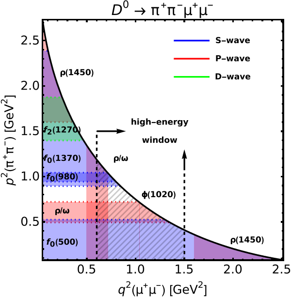
Figure 1: Phase space allowed in the decay $D^{0}\to\pi^{+}\pi^{-}\mu^{+}\mu^{-}$; the invariant mass of the pion (muon) pair is denoted $p^{2}$ (respectively, $q^{2}$). Some scalar (blue), vectorial (red) and tensorial (green) resonant contributions are shown (the very narrow pseudoscalar resonances $\eta^{(}{{}^{\prime}}{}^{)}$, leading to the lepton pair via two-photon exchange, are omitted); the bands correspond to $(m\pm\Gamma/2)^{2}$, with $\Gamma$ taken from Refs. [34, 24, 35, 25]. The “high-energy window” referred to in the plot corresponds to $m_{\rho^{0}}^{2}\lesssim q^{2}\lesssim 1.5$ GeV², for which only $f_{0}(500)\equiv\sigma$ gives an important contribution among the $S$-wave contributions, and is indicated by a hashed pattern delimited by dashed vertical lines. Cascade decays are not indicated.

Concerning other rare charm-meson decay modes with pion pairs in the final state, we note that the channel $D^{\pm}\to\pi^{\pm}\pi^{0}\ell^{+}\ell^{-}$ is not sensitive to the $S$-wave contributions under discussion and is experimentally more challenging. The mode $D^{0}\to\pi^{0}\pi^{0}\ell^{+}\ell^{-}$ (which does not receive contributions of the $P$-wave, following Bose-Einstein symmetry) represents an even more significant experimental challenge. These decay modes will thus not be discussed in the following. Limits on the electronic mode $D^{0}\to\pi^{+}\pi^{-}e^{+}e^{-}$ branching ratio are discussed in Refs. [36, 37].

Before concluding this introduction, let us point out that the $S$-wave contribution is relevant also in the bottom sector. For a discussion in the case of $B^{0}\to K^{+}\pi^{-}\ell^{+}\ell^{-}$, where the $S$-wave contamination from $B^{0}\to K^{\ast}_{0}(\to K^{+}\pi^{-})\ell^{+}\ell^{-}$ in the reconstruction of the decay chain is at the level of $\approx 10\%$, see Refs. [44, 45, 46, 47, 48, 49, 50]; note that LHCb has performed measurements of the $S$-wave contribution, e.g., in Refs. [51, 52]. In the cases of scalar isoscalar states, the $S$-wave has been discussed for $B_{(s)}\to\pi\pi J/\psi$ [53, 54, 55], which contributes to $B_{(s)}\to\pi\pi\ell^{+}\ell^{-}$; note that the $\sigma$ is expected to provide a sizable contribution, naively as large as $\approx 26\%$, and thus coincident with the result of BESIII [26] in the charm-sector, since $\mathcal{B}(B^{0}\to\rho^{0}J/\psi(1S))\simeq 2.6\times 10^{-5}$ [56, 57], while $\mathcal{B}(B^{0}\to\sigma J/\psi(1S))\simeq 0.9\times 10^{-5}$ [56]. A process related to the final state with pion pairs is $B_{(s)}\to KK\ell^{+}\ell^{-}$ [44, 47, 48], due to final-state rescattering [53, 54, 55]. Important contributions of the $S$-wave are in principle also to be expected in semi-leptonic decays $B^{+}\to\pi\pi\ell^{+}\nu_{\ell}$ ($\ell=e,\mu,\tau$) [58, 59], and should then be taken into account in future tests of the SM, such as lepton flavour universality; see Ref. [60] for a discussion of the extraction of the $P$-wave contribution from a lattice QCD calculation. See Refs. [61, 62, 63, 64] for discussions of the $S$-wave contribution to $\bar{B}\to D\pi\ell\bar{\nu}_{\ell}$.

This article is organized as follows: in Sec. 2 we formalize the inclusion of intermediate resonances; then, in Sec. 3 we discuss the theoretical expressions of distinct observables; finally, in Sec. 4 we present our numerical comparisons with available data; conclusions are provided in Sec. 5. In App. A we give the expressions of the line-shapes in use, among further useful hadronic information, and some further comparisons regarding Ref. [26] are given in App. B.

2 Inclusion of intermediate resonances in naive factorization

To start, we introduce the Single Cabibbo Suppressed (SCS) effective interaction Hamiltonian density for $\Delta C=1$ up to operators of dimension-six, valid for energy scales $\mu<\mu_{b}$ ($\mu_{b}$ being the energy scale at which the bottom-quark is integrated out) [65]:

$$\mathcal{H}_{\rm eff}=\frac{G_{F}}{\sqrt{2}}\left[\,\sum^{2}_{i=1}C_{i}(\mu)\left(\lambda_{d}Q_{i}^{d}+\lambda_{s}Q_{i}^{s}\right)-\lambda_{b}\left(C_{7}(\mu)Q_{7}+C_{9}(\mu)Q_{9}+C_{10}(\mu)Q_{10}\right)\right]+\mathrm{h.c.}$$ (2)

where

$$\lambda_{q}=V^{\ast}_{cq}V_{uq}\,,\qquad q=d,s,b\,.$$ (3)

The basis of operators is the following:

$$Q_{1}^{d}=(\overline{d}c)_{V-A}(\overline{u}d)_{V-A}\,,$$ (4)

$$Q_{2}^{d}=(\overline{d}_{j}c_{i})_{V-A}(\overline{u}_{i}d_{j})_{V-A}\stackrel{{\scriptstyle[}}{{]}}{Fierz}{=}(\overline{u}c)_{V-A}(\overline{d}d)_{V-A}\,,$$

$$Q_{1}^{s}=(\overline{s}c)_{V-A}(\overline{u}s)_{V-A}\,,$$

$$Q_{2}^{s}=(\overline{s}_{j}c_{i})_{V-A}(\overline{u}_{i}s_{j})_{V-A}\stackrel{{\scriptstyle[}}{{]}}{Fierz}{=}(\overline{u}c)_{V-A}(\overline{s}s)_{V-A}\,,$$

$$Q_{7}=\frac{e}{8\pi^{2}}m_{c}\overline{u}\sigma_{\mu\nu}(\mathbf{1}+\gamma_{5})F^{\mu\nu}c\,,$$

$$Q_{9}=\frac{\alpha_{em}}{2\pi}(\overline{u}\gamma_{\mu}(\mathbf{1}-\gamma_{5})c)(\overline{\ell}\gamma^{\mu}\ell)\,,$$

$$Q_{10}=\frac{\alpha_{em}}{2\pi}(\overline{u}\gamma_{\mu}(\mathbf{1}-\gamma_{5})c)(\overline{\ell}\gamma^{\mu}\gamma_{5}\ell)\,,$$

where $(V-A)_{\mu}=\gamma_{\mu}(\mathbf{1}-\gamma_{5})$, $i,j$ are colour indices, and $\mu\sim\overline{m}_{c}(\overline{m}_{c})$ is the renormalization scale. The operators $Q_{i}^{q}$, $q=d,s$ and $i=1,2$, are the current-current operators. Above, we have not kept contributions in $\lambda_{b}$ other than the electromagnetic dipole $Q_{7}$ and the semi-leptonic interactions $Q_{9}$ and $Q_{10}$, which are kept for the only sake of later convenience. The (short-distance) SM Wilson coefficients $C_{7},C_{9},C_{10}$, first generated at one-loop via the exchange of EW gauge bosons, are significantly suppressed in the $D$ system [66], and furthermore their contributions are accompanied with a CKM suppression; since $C_{10}\sim 0$ in the SM, we will see that some angular observables approximately vanish (i.e., those based in $I_{5,6,7}$). The main SM contribution to an effective $C_{9}$ comes from long-distance dynamics, as it will be later discussed in this section. As stressed in Ref. [14], the latter feature is welcomed in the sense that it enhances the sensitivity to NP that contributes to the observables that vanish in the SM, such as having $Q_{10}$ induced by NP which interferes with the large SM long-distance part. Operators of flipped chirality, i.e., $Q_{7}^{\prime},Q_{9}^{\prime},Q_{10}^{\prime}$, are not displayed, and are virtually absent in the SM, their contributions being relatively suppressed by $m_{u}/m_{c}$. For all purposes, we take $\lambda_{s}=-\lambda_{d}$.

The full decay amplitude of the charm-meson decay is calculated here in the framework of factorization, closely following Ref. [13]. We include in our analysis only the quasi two-body topologies with the lowest lying intermediate resonances that are indicated in Fig. 2. Therein, the lepton pair originates from one vector meson, namely, $\rho^{0}$, $\omega$, or $\phi$, coupling to a photon (we neglect cases where one isoscalar hadron couples to two photons due to the small resulting effect, as supported by data, see e.g. Ref. [68]; similarly, we do not include pseudoscalar resonances in our analysis). The pion pair originates from strong decays of $\rho^{0}$, $\omega$, or $\sigma$. The latter list does not include the $\phi$ since we assume the Zweig rule to be at play, i.e., we discard the possibility of a light-quark pair rescattering into $s\overline{s}$. Since the intermediate resonances are electrically neutral, the only operators that contribute in naive factorization are $Q_{2}^{q}$, $q=d,s$. We employ the next-to-leading order (NLO) value $C_{2}=-0.40$ in the naive dimensional regularization (NDR) scheme at $m_{c}$ [65, 66].

We write schematically for the $S$-matrix element of the process:

$$\qquad\qquad\langle\pi^{+}\pi^{-}\ell^{+}\ell^{-}|S|D^{0}\rangle$$ (5)

$$=\langle\pi^{+}\pi^{-}\ell^{+}\ell^{-}|\int d^{4}x\,d^{4}w\,d^{4}y\,d^{4}z\,T\{\mathcal{H}_{em}^{\rm lept}(z)\,\mathcal{H}_{\mathcal{V}\gamma}(y)\,\mathcal{H}_{\mathcal{R}\pi\pi}(w)\,\mathcal{H}_{D\mathcal{R}\mathcal{V}}(x)\}|D^{0}\rangle\,,$$

with electromagnetic interactions given by [69]:

$$\mathcal{H}_{\mathcal{V}\gamma}=-e\,\left(\frac{f_{\rho^{0}}}{\sqrt{2}m_{\rho^{0}}}\left(\rho^{0}\right)^{\mu}\,+\frac{1}{3}\frac{f_{\mathcal{\omega}}}{\sqrt{2}m_{\mathcal{\omega}}}\,\mathcal{\omega}^{\mu}-\frac{\sqrt{2}}{3}\frac{f_{\mathcal{\phi}}}{\sqrt{2}m_{\mathcal{\phi}}}\,\mathcal{\phi}^{\mu}\right)\,\square A_{\mu}\,,\qquad\mathcal{H}_{em}^{\rm lept}=e\,A^{\mu}\,\overline{\ell}\gamma_{\mu}\ell\,.$$ (6)

Above, $\mathcal{R}$ is one of the vector or scalar resonances coupling to the pion pair, and $\mathcal{V}$ is the vector resonance coupling electromagnetically to the lepton pair. The flavour changing interaction $\mathcal{H}_{D\mathcal{R}\mathcal{V}}$ results from insertions of the current-current operators $Q_{2}^{q}$, $q=d,s$, of the weak Hamiltonian density in Eq. (2), while matrix elements of $\mathcal{H}_{\mathcal{R}\pi\pi}$ are discussed in Secs. 2.1 and 2.2 for intermediate vectors and the scalar, respectively.

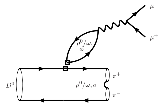
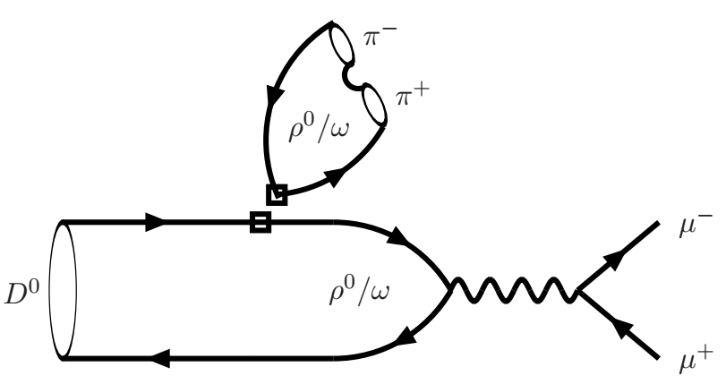
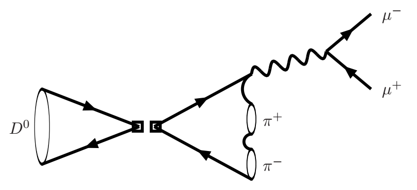
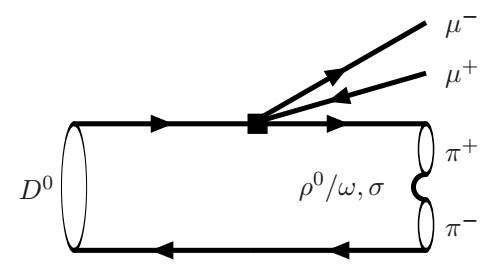
Figure 2: Quasi two-body topologies; the lepton (pion) pair comes from electromagnetic (respectively, strong) decays of the intermediate resonances; (Top, Left) W-type factorization contribution, (Top, Right) J-type factorization contribution, (Bottom, Left) A-type factorization contribution (i.e., annihilation topology); pairs of empty squares represent the two quark colour-neutral bilinears that are factorized. (Bottom, Right) Contributions for which the lepton pair comes from an effective semi-leptonic contact interaction, represented by a solid square.

Let us at this point define the specific topologies that show up within factorization given the intermediate states aforementioned. There are three possible ways to contract the currents, shown graphically in Fig. 2:

$$Q_{A}\equiv-\braket{\mathcal{R}\mathcal{V}}{(\overline{q}q)_{V-A}}{0}\braket{0}{\overline{u}\gamma^{\mu}\gamma_{5}c}{D^{0}(p_{D})}=\braket{\mathcal{R}\mathcal{V}}{(\overline{q}q)_{A}(x)}{0}if_{D}p_{D}^{\mu}\,e^{-i\,p_{D}\cdot x}\,,$$ (7)

$$Q_{W}\equiv\left\{\begin{array}[]{l}\braket{\mathcal{V}}{(\overline{q}q)_{V}}{0}\braket{\mathcal{R}}{(\overline{u}c)_{V-A}}{D^{0}}\,,\quad\mathcal{R}=\rho^{0},\omega\,,\\ \\ -\braket{\mathcal{V}}{(\overline{q}q)_{V}}{0}\braket{\mathcal{R}}{(\overline{u}c)_{A}}{D^{0}}\,,\quad\mathcal{R}=\sigma\,,\end{array}\right.$$ (8)

$$Q_{J}\equiv\braket{\mathcal{R}}{(\overline{q}q)_{V}}{0}\braket{\mathcal{V}}{(\overline{u}c)_{V-A}}{D^{0}}\,,\quad\mathcal{R}=\rho^{0},\omega\,,$$ (9)

where $q=d,s$. Both quark bilinears are calculated at the same space-time point. Above, we have already indicated explicitly which currents (whether vector, axial-vector, or both) give non-vanishing contributions, and which resonances are possible. In particular, note that there is no $\sigma$ exchange in the $Q_{J}$ case, since the (axial)vector $\braket{\sigma}{(\overline{q}q)_{V(A)}}{0}$ matrix element vanishes. The type of contraction at the origin of $Q_{A}$, which is the weak annihilation topology, is proportional to the light quark mass $m_{q}$, as seen from contracting the axial-vector current $\overline{q}\gamma_{\mu}\gamma_{5}q$ with the decaying charm-meson four-momentum $p_{D}^{\mu}$, and we will thus neglect this contribution compared to the other two, that are non-zero; see e.g. Ref. [70] for a discussion.

We are left with the types of contractions of $Q_{W}$ and $Q_{J}$, that we shall refer to as ‘W’- and ‘J’-type contractions, and to which we now turn and provide further details. In the case of W-type factorization, we need to evaluate the following vacuum to lepton pair matrix element:

$$\braket{\ell^{+}\ell^{-}}{\int d^{4}y\,d^{4}z\,T\left\{\mathcal{H}_{em}^{\rm lept}(z)\,\mathcal{H}_{\mathcal{V}\gamma}(y)\,\left(\sum_{q=d,s}\lambda_{q}(\overline{q}q)_{V}(x)\right)\right\}}{0}$$ (10)

$$\quad=-\sum_{\mathcal{V}=\rho^{0},\omega,\phi}\braket{\ell^{+}\ell^{-}}{H_{em}^{\rm lept}}{\gamma^{\ast}}\frac{1}{q^{2}}\braket{\gamma^{\ast}}{H_{\mathcal{V}\gamma}}{\mathcal{V}}\frac{1}{P_{\mathcal{V}}(q^{2})}\braket{\mathcal{V}}{\sum_{q=d,s}\lambda_{q}(\overline{q}q)_{V}(x)}{0}$$

$$\quad\quad=-e^{iq\cdot x}\lambda_{d}e^{2}\,(\overline{u}_{\ell}\gamma^{\mu}v_{\ell})\left(\frac{c^{W}_{\rho^{0}}\,f_{\rho^{0}}^{2}}{P_{\rho^{0}}(q^{2})}+\frac{c^{W}_{\omega}\,f_{\omega}^{2}}{P_{\omega}(q^{2})}+\frac{c^{W}_{\phi}\,f_{\phi}^{2}}{P_{\phi}(q^{2})}\right)\,,$$

where $q^{2}$ is the invariant mass squared of the lepton pair, and $c^{W}_{\rho^{0}}=1/2$, $c^{W}_{\omega}=-1/6$ and $c^{W}_{\phi}=-1/3$. The expressions for the line-shapes will be later discussed in the text (see App. A.3). Note that the $\phi$ contribution comes with the CKM factor $\lambda_{s}$, where $\lambda_{s}=-\lambda_{d}$. For the values of the decay constants, see App. A.1.

In the J-type factorization, we need to evaluate the following $D^{0}\to\ell^{+}\ell^{-}$ matrix element:

$$\braket{\ell^{+}\ell^{-}}{\int d^{4}y\,d^{4}z\,T\left\{\mathcal{H}_{em}^{\rm lept}(z)\,\mathcal{H}_{\mathcal{V}\gamma}(y)\,\lambda_{d}(\overline{u}\gamma_{\mu}c)(x)\right\}}{D^{0}(p_{D})}$$

$$\quad=-\sum_{\mathcal{V}=\rho^{0},\omega}\braket{\ell^{+}\ell^{-}}{H_{em}^{\rm lept}}{\gamma^{\ast}}\frac{1}{q^{2}}\braket{\gamma^{\ast}}{H_{\mathcal{V}\gamma}}{\mathcal{V}}\frac{1}{P_{\mathcal{V}}(q^{2})}\braket{\mathcal{V}}{\lambda_{d}(\overline{u}\gamma_{\mu}c)(x)}{D^{0}(p_{D})}$$

$$\quad\quad=-e^{i(q-p_{D})\cdot x}\lambda_{d}e^{2}\,(\overline{u}_{\ell}\gamma_{\mu}v_{\ell})\left(\frac{c^{J}_{\rho^{0}}\,f_{\rho^{0}}}{m_{\rho^{0}}P_{\rho^{0}}(q^{2})}+\frac{c^{J}_{\omega}\,f_{\omega}}{m_{\omega}P_{\omega}(q^{2})}+\frac{c^{J}_{\phi}\,f_{\phi}}{m_{\phi}P_{\phi}(q^{2})}\right)$$

$$\quad\quad\quad\times(A_{1}(p^{2})\,c_{1}(q^{2},p^{2})+A_{2}(p^{2})\,c_{2}(q^{2},p^{2})+V(p^{2})\,c_{V}(q^{2},p^{2})+A_{0}(p^{2})c_{0}(q^{2},p^{2}))\,,$$

where $p^{2}$ is the invariant mass squared of the pion pair, and $c^{J}_{\rho^{0}}=1/\sqrt{2}$, $c^{J}_{\omega}=+1/(3\sqrt{2})$ and $c^{J}_{\phi}=0$. Again, the $\phi$ does not contribute due to its quark content (similarly, there is no contribution proportional to $\lambda_{s}$). The form factors of $D\to\mathcal{V}$, $\mathcal{V}=\rho^{0},\omega$, are equal for the two resonances (see App. A.2 for details about their parameterizations); the functions $c_{i}(q^{2},p^{2})$, $i=V,0,1,2$, encode the kinematical factors that accompany each form factor [71].

In the above Eqs. (10) and (2), the relative signs and numerical prefactors between $\rho^{0}$ and $\omega$ can be quickly understood from the quark content of the vector resonances

$$V_{\mu}^{\phi}\equiv\bar{s}\gamma_{\mu}s\,,\;\;V_{\mu}^{\omega}\equiv\frac{1}{\sqrt{2}}\left(\bar{u}\gamma_{\mu}u+\bar{d}\gamma_{\mu}d\right)\,,\;\;V_{\mu}^{\rho^{0}}\equiv\frac{1}{\sqrt{2}}\left(\bar{u}\gamma_{\mu}u-\bar{d}\gamma_{\mu}d\right)\,,\;\;$$ (12)

where the quark content of the operators $V_{\mu}^{\mathcal{V}}$ is such that they can create or annihilate the vector meson $\mathcal{V}$, and we enforce the Zweig rule (for corrections, see e.g. Ref. [72]). In terms of these operators, the hadronic electromagnetic current can be rewritten as:

$$(j_{em}^{\rm had})_{\mu}=Q_{s}\,V_{\mu}^{\phi}+\frac{Q_{u}+Q_{d}}{\sqrt{2}}\,V_{\mu}^{\omega}+\frac{Q_{u}-Q_{d}}{\sqrt{2}}\,V_{\mu}^{\rho^{0}}\,,$$ (13)

where $Q_{u}=+2/3$ and $Q_{d}=Q_{s}=-1/3$.

To accommodate further strong dynamics, we will in the following discussion associate a strong phase $\delta_{\{\mathcal{R},\mathcal{V}\}}$ to each vertex $\braket{\mathcal{R}\mathcal{V}}{\mathcal{H}_{D\mathcal{R}\mathcal{V}}}{D^{0}}$; a similar approach is followed by Ref. [14]; see also Ref. [16] (strong phases are extracted from $e^{+}e^{-}$ data in Refs. [73, 16]). It will be assumed that these strong phases vary slowly, the faster variations being expected from the line shapes, and one then takes the $\delta_{\{\mathcal{R},\mathcal{V}\}}$ as constants under the assumption that the main resonances needed for phenomenological applications are included in our analysis. Such strong phases are introduced to represent rescattering effects that take place beyond (naive) factorization. This leaves us with six arbitrary phases for the couplings of $D^{0}$ to $\rho^{0}-\rho^{0}$, $\rho^{0}-\omega$, $\rho^{0}-\phi$, $\sigma-\rho^{0}$, $\sigma-\omega$ and $\sigma-\phi$ pairs of resonances. We will shortly discuss the phases present in $D^{0}$ to $\omega-\rho^{0}$, $\omega-\omega$, $\omega-\phi$ (see the discussion following Eq. (18) below). In practice, we will see that the presently measured $d\Gamma/dq^{2}$ distribution depends on the phase differences:

$$\Delta_{1}\equiv\delta_{\{\rho^{0}/\omega,\rho^{0}\}}-\delta_{\{\rho^{0}/\omega,\phi\}}\,,\quad\Delta_{2}\equiv\delta_{\{\rho^{0}/\omega,\rho^{0}\}}-\delta_{\{\rho^{0}/\omega,\omega\}}\,,$$ (14)

$$\Delta_{3}\equiv\delta_{\{\sigma,\rho^{0}\}}-\delta_{\{\sigma,\phi\}}\,,\quad\quad\Delta_{4}\equiv\delta_{\{\sigma,\rho^{0}\}}-\delta_{\{\sigma,\omega\}}\,,$$

since $S$- and $P$-waves do not interfere in $d\Gamma/dq^{2}$; given that the $\omega$ and $\phi$ are narrow resonances, $\Delta_{1}-\Delta_{2}$ and $\Delta_{3}-\Delta_{4}$ do not play an important role. On the other hand, when discussing angular observables that depend on the $S$- and $P$-waves interference, the following extra phase difference is relevant:

$$\Delta_{SP}\equiv\delta_{\{\sigma,\rho^{0}\}}-\delta_{\{\rho^{0}/\omega,\rho^{0}\}}\,,$$ (15)

which completes the list of phase differences in the SM to be discussed below (i.e., out of six phases we have five independent differences among them).

2.1 Implementation of the $\pi^{+}\pi^{-}$ $P$-wave contribution

For the coupling of a vector resonance $V$ to the pion pair we use the following expression for the matrix element of $H_{\mathcal{R}\pi\pi}$ resulting from strong interactions:

$$\bra{\pi^{+}(p_{1})\pi^{-}(p_{2})}H_{\mathcal{R}\pi\pi}\ket{V(p,\lambda)}=F_{BW}(p^{2})\,b_{V}\,\epsilon_{V}(p,\lambda)\cdot(p_{1}-p_{2})\,,$$ (16)

where the phenomenological form factor $F_{BW}$ is the so-called Blatt-Weisskopf barrier factor for a particle of spin-1; see App. A.3 for definitions, and the review on resonances of Ref. [25]. The quantity $b_{V}$ is assumed not to carry any dynamics, and is extracted from the decay rate of $V\rightarrow\pi^{+}\pi^{-}$:

$$\Gamma(V\rightarrow\pi^{+}\pi^{-})=\frac{1}{48\pi}b_{V}^{2}m_{V}^{-5}\lambda^{3/2}(m_{V}^{2},m_{\pi}^{2},m_{\pi}^{2})\,,$$ (17)

where $\lambda(a,b,c)=a^{2}+b^{2}+c^{2}-2(ab+bc+ca)$. In practice this relation is used only for $V=\rho^{0}$, for which we take $\mathcal{B}(\rho^{0}\rightarrow\pi^{+}\pi^{-})=1$, thus resulting in $b_{\rho^{0}}=5.92$.

The line-shape of $\rho^{0}$ is expressed in the Gounaris-Sakurai parameterisation [74], which implements finite-width corrections (see App. A.3 for details). Following previous literature on $\rho^{0}/\omega$ contributions to $e^{+}e^{-}\to\pi^{+}\pi^{-}$, we collect both resonances together by considering the expression:

$$b_{\rho^{0}/\omega}(p^{2})=b_{\rho^{0}}\left(1+a_{\omega}\,e^{i\phi_{\omega}}\,\text{RBW}_{\omega}(p^{2})\right)\,,$$ (18)

where the relativistic Breit-Wigner line-shape $\text{RBW}_{\omega}(s)$ is given in App. A.3. In (naive) factorization, if only the W-type contraction was possible, then $\phi_{\omega}=0$; on the contrary, in the J-type contraction, $\phi_{\omega}=\pi$. In Eq. (18), both contributions are collected together, and the phase $\phi_{\omega}$ will also accommodate further hadronic effects beyond (naive) factorization in our study. In Sec. 4, the parameters $a_{\omega}$ and $\phi_{\omega}$ of the coupling of the $\omega$ to two pions are fitted to the experimental differential branching ratio as a function of the invariant mass of the pion pair (a small but non-vanishing value of $a_{\omega}$ is generated from isospin-breaking effects, mixing the isospin-triplet $\rho$ and the isospin-singlet $\omega$ states). This is different from the implementation of the resonances in the matrix elements of the lepton pair, where the ${\rho^{0}}$ and $\omega$ contributions are added serially. We then have for the contribution where the pion pair originates from ${\rho^{0}}/\omega$ resonances:

$$\braket{\pi^{+}\pi^{-}\ell^{+}\ell^{-}}{S}{D^{0}}^{({\rho^{0}}/\omega)}=(2\pi)^{4}\,\delta^{(4)}(p+q-p_{D})\,\xi_{2}\frac{b_{{\rho^{0}}/\omega}(p^{2})F_{BW}(p^{2})}{P_{\rho^{0}}(p^{2})}(\overline{u}_{\ell}\gamma_{\mu}v_{\ell})$$

$$\;\times\sum_{\mathcal{V}}\Bigg{\{}\left[\frac{c^{W}_{\mathcal{V}}B_{\mathcal{V}}f_{\mathcal{V}}^{2}e^{i\delta_{\{{\rho^{0}/\omega},\mathcal{V}\}}}}{P_{\mathcal{V}}(q^{2})}\left(\frac{2q\cdot(p_{1}-p_{2})}{m_{D}+\sqrt{p^{2}}}A_{2}(q^{2})-\left(m_{D}+\sqrt{p^{2}}\right)A_{1}(q^{2})\right)\right.$$

$$\;\;\left.+\frac{1}{\sqrt{2}}m_{\rho^{0}}f_{\rho^{0}}\frac{c^{J}_{\mathcal{V}}B_{\mathcal{V}}f_{\mathcal{V}}e^{i\delta_{\{{\rho^{0}/\omega},\mathcal{V}\}}}}{m_{\mathcal{V}}P_{\mathcal{V}}(q^{2})}\left(\frac{2q\cdot(p_{1}-p_{2})}{m_{D}+\sqrt{q^{2}}}A_{2}(p^{2})-\left(m_{D}+\sqrt{q^{2}}\right)A_{1}(p^{2})\right)\right]p_{1}^{\mu}$$

$$\;\;\;+\left[\frac{c^{W}_{\mathcal{V}}B_{\mathcal{V}}f_{\mathcal{V}}^{2}e^{i\delta_{\{{\rho^{0}/\omega},\mathcal{V}\}}}}{P_{\mathcal{V}}(q^{2})}\left(\frac{2q\cdot(p_{1}-p_{2})}{m_{D}+\sqrt{p^{2}}}A_{2}(q^{2})+\left(m_{D}+\sqrt{p^{2}}\right)A_{1}(q^{2})\right)\right.$$

$$\;\;\;\;\left.+\frac{1}{\sqrt{2}}m_{\rho^{0}}f_{\rho^{0}}\frac{c^{J}_{\mathcal{V}}B_{\mathcal{V}}f_{\mathcal{V}}e^{i\delta_{\{{\rho^{0}/\omega},\mathcal{V}\}}}}{m_{\mathcal{V}}P_{\mathcal{V}}(q^{2})}\left(\frac{2q\cdot(p_{1}-p_{2})}{m_{D}+\sqrt{q^{2}}}A_{2}(p^{2})+\left(m_{D}+\sqrt{q^{2}}\right)A_{1}(p^{2})\right)\right]p_{2}^{\mu}$$

$$\;\;\;\;\;+\left[\frac{c^{W}_{\mathcal{V}}B_{\mathcal{V}}f_{\mathcal{V}}^{2}e^{i\delta_{\{{\rho^{0}/\omega},\mathcal{V}\}}}}{P_{\mathcal{V}}(q^{2})}\frac{-4iV(q^{2})}{m_{D}+\sqrt{p^{2}}}\right.$$

$$\;\;\;\;\;\;\left.+\frac{1}{\sqrt{2}}m_{\rho^{0}}f_{\rho^{0}}\frac{c^{J}_{\mathcal{V}}B_{\mathcal{V}}f_{\mathcal{V}}e^{i\delta_{\{{\rho^{0}/\omega},\mathcal{V}\}}}}{m_{\mathcal{V}}P_{\mathcal{V}}(q^{2})}\frac{-4iV(p^{2})}{m_{D}+\sqrt{q^{2}}}\right]\epsilon^{\mu\nu\lambda{\rho}}p_{1\nu}p_{2\lambda}q_{\rho}\Bigg{\}}\,,$$ (19)

where

$$\xi_{2}=\lambda_{d}\frac{G_{F}}{\sqrt{2}}e^{2}C_{2}(\mu)\,.$$ (20)

The terms coming with $A_{1}(q^{2})$, $A_{2}(q^{2})$, $V(q^{2})$ (respectively, $A_{1}(p^{2})$, $A_{2}(p^{2})$, $V(p^{2})$) originate from the W-type (J-type) factorization, since the momentum transfer of the $D^{0}$ form factor is the one of the lepton pair (pion pair). Note that the $A_{0}$ contribution vanishes because it is accompanied by $q^{\mu}\overline{\ell}\gamma_{\mu}\ell=0$ in the W-type factorization, and by $p_{1}^{2}-p_{2}^{2}$ in the J-type factorization, also vanishing in the case of $\pi^{+}\pi^{-}$ final-state mesons. In the case of charm-meson decays the J-type contribution gives sizeable effects, as it is manifest from Eq. (2.1).

In Eq. (2.1), apart from the complex phases that correct the (naive) factorization picture, we have also introduced for the same sake the real and positive parameters $B_{\rho^{0}}$, $B_{\omega}$ and $B_{\phi}$ that will be adjusted from data, and are also assumed not to carry any dependence with the energy. Note that a somewhat similar approach is followed by Ref. [14], which fits the factors controlling the normalizations of the resonances around their respective peaks.

2.2 Implementation of the $\pi^{+}\pi^{-}$ $S$-wave contribution

We now consider the effect of the $\sigma=f_{0}(500)$ resonance. The $\sigma$ is encoded in the $w_{+}$ and $r$ form-factors of the $D^{0}\to\pi^{+}\pi^{-}$ matrix element [71, 75, 76]:

$$\braket{\pi^{+}(p_{1})\pi^{-}(p_{2})}{(\overline{u}\gamma^{\mu}(1-\gamma_{5}){c})(x)}{D^{0}(p_{D})}=e^{ix\cdot(p-p_{D})}\{iw_{+}(p_{1}+p_{2})^{\mu}$$

$$\qquad+iw_{-}(p_{1}-p_{2})^{\mu}+h\epsilon^{\mu\alpha\beta\gamma}(p_{D})_{\alpha}(p_{1}+p_{2})_{\beta}(p_{1}-p_{2})_{\gamma}+irq^{\mu}\}\,.$$ (21)

The contraction of $q^{\mu}$ with the spinorial part of the leptonic matrix element $(\overline{u}_{\ell}\gamma^{\mu}v_{\ell})$ in Eq. (10) vanishes, and thus the effect of the $S$-wave intermediate states appears only in the form factor $w_{+}$, to which the following $S$-wave term is added:

$$w^{S}_{+}(p^{2},q^{2})=a_{S}(q^{2})\mathcal{A}_{S}(p^{2})\,,\quad a_{S}(q^{2})=a_{S}(0)/\left(1-\frac{q^{2}}{m_{A}^{2}}\right)\,.$$ (22)

Here, the nearest pole is used [26], for which we have $m_{A}=2.42$ GeV, where $A$ is the axial $D$-meson ($J^{P}=1^{+}$). The quantity $a_{S}(0)$, assumed to be a constant, represents a magnitude encompassing the strength of the transition $D\rightarrow\sigma$ multiplied by the coupling of $\sigma$ to the pion pair. We extract it from fitting the experimental data. Following Ref. [26], the lineshape $\mathcal{A}_{S}(p^{2})$ is the one of Bugg [23], which is data-driven (and in particular includes small Zweig-violating effects); its full expression is provided in App. A.3. The complex phase assigned to the $\sigma$ is close to the one extracted from $\pi\pi$ rescattering in the elastic region. We reserve the analysis of alternative line-shapes to the future when the quest of higher precision may become more pressing.

With all the above, we incorporate the scalar resonance to our factorization model

$$\langle\pi^{+}\pi^{-}\ell^{+}\ell^{-}|S|D^{0}\rangle^{(\sigma)} = (2\pi)^{4}\,\delta^{(4)}(p+q-p_{D})\,\xi_{2}(\overline{u}_{\ell}\gamma_{\mu}v_{\ell})i$$

$$\qquad\times\sum_{\mathcal{V}}\frac{c^{W}_{\mathcal{V}}B_{\mathcal{V}}^{(S)}f_{\mathcal{V}}^{2}e^{i\delta_{\{\sigma,\mathcal{V}\}}}}{P_{\mathcal{V}}(q^{2})}a_{S}(q^{2})\mathcal{A}_{S}(p^{2})\,.$$

The full matrix element is then given by

$$\langle\pi^{+}\pi^{-}\ell^{+}\ell^{-}|S|D^{0}\rangle=\braket{\pi^{+}\pi^{-}\ell^{+}\ell^{-}}{S}{D^{0}}^{({\rho^{0}}/\omega)}+\langle\pi^{+}\pi^{-}\ell^{+}\ell^{-}|S|D^{0}\rangle^{(\sigma)}\,.$$ (24)

2.3 Effective Wilson coefficient

It would be useful to write the previous matrix element in Eq. (24) as the matrix element of a semi-leptonic four-fermion operator, with the intermediate resonance at the origin of the lepton pair encoded in an effective Wilson coefficient. Assuming that the only factorization is the W-type one, as is the case for instance in semi-leptonic non-rare decays, it is easy to match the full hadronic matrix element to that of a $Q_{9}$ operator, i.e., in which the quark pair carries the chiral $V-A$ structure, and the lepton pair a vector structure, as it would result from the coupling to a single photon. As seen from Eqs. (8) and (10), the matrix element $\langle\pi^{+}\pi^{-}|(\bar{u}c)_{V-A}(x)|D^{0}\rangle$ for initial and final state mesons has been factorized out from the leptonic matrix element, and we are able to write the latter as $\langle\ell^{+}\ell^{-}|(\bar{\ell}\ell)_{V}(x)|0\rangle$ times an effective coefficient that encodes the intermediate resonant dynamics of the lepton pair invariant mass

$$C^{{\rm eff}:W}_{9}(\mu;q^{2}) = 8\pi^{2}C_{2}(\mu)\left(\frac{c^{W}_{\rho^{0}}f_{\rho^{0}}^{2}}{P_{\rho^{0}}(q^{2})}B_{\rho^{0}}e^{i\delta_{\{{\rho^{0}/\omega},{\rho^{0}}\}}}\right.$$

$$\;\;+\left.\frac{c^{W}_{\omega}f_{\omega}^{2}}{P_{\omega}(q^{2})}B_{\omega}e^{i\delta_{\{{\rho^{0}/\omega},{\omega}\}}}+\frac{c^{W}_{\phi}f_{\phi}^{2}}{P_{\phi}(q^{2})}B_{\phi}e^{i\delta_{\{{\rho^{0}/\omega},{\phi}\}}}\right)$$

(where we have included the factors beyond (naive) factorization that have been previously discussed), such that the transition $c\to u\ell^{+}\ell^{-}$ is described by

$$\mathcal{H}^{c\to u\ell\ell}_{\rm eff}=\frac{G_{F}}{\sqrt{2}}\lambda_{d}C_{9}^{{\rm eff}:W}(\mu;q^{2})Q_{9}+\mathrm{h.c.}$$ (26)

Conversely, the matrix element appearing in the J-type contribution is $\langle\mathcal{V}|(\bar{u}c)_{V-A}|D^{0}\rangle$, where $\mathcal{V}$ does not lead to the pion pair, but instead to the lepton pair, so we cannot separate the full matrix element into a hadronic times a leptonic factors calculated at the same space-time point. Thus this contribution prevents us from writing, at least straightforwardly, our full amplitude using an effective Wilson coefficient multiplying a semi-leptonic four-fermion operator.

In the following we explore an alternative which would make the use of an approximate effective $C_{9}$ coefficient viable, if the $\rho^{0}/\omega$ were the only resonances creating the pion pair. Starting with the $\rho^{0}$, we rewrite the J- and W-type contributions in a way that approximates an effective coefficient for $Q_{9}$. By inspecting Eq. (2.1), one condition is that

$$m_{\rho^{0}}f_{\rho^{0}}\frac{f_{\rho^{0}}}{m_{\rho^{0}}P_{\rho^{0}}(q^{2})}\frac{1}{m_{D}+\sqrt{q^{2}}}F(p^{2})\simeq\frac{f_{\rho^{0}}^{2}}{P_{\rho^{0}}(q^{2})}\frac{1}{m_{D}+\sqrt{p^{2}}}F(q^{2})\,,\;F=A_{2},V\,,$$ (27)

while a similar discussion holds for the terms that are proportional to the form factor $A_{1}$. To achieve our goal, we need firstly to examine if the $m_{D}+\sqrt{q^{2}}$ and $m_{D}+\sqrt{p^{2}}$ factors can be replaced with $m_{D}+m_{\rho}$, as it is usually done in the literature. Indeed, this narrow-width approximation is good enough. What is left of the above conditions in Eq. (27) comes from the dependencies of the form factors on $q^{2}$ or $p^{2}$. Since in our nearest pole parameterisation of the form factors in App. A.2 these dependencies go as ${m_{\rm pole}^{2}}/({m_{\rm pole}^{2}}-{q^{2}})$ or ${m_{\rm pole}^{2}}/({m_{\rm pole}^{2}}-{p^{2}})$, and the di-lepton and di-hadron invariant masses are generally much smaller than the pole masses, the two dependencies are soft.

The situation is more complicated for the $\omega$. Since $c^{W}_{\omega}$ and $c^{J}_{\omega}$ have opposite signs, seemingly the $\omega$ contribution in the leptonic part would disappear in Eq. (2.1) under the use of the simplifications discussed in the previous paragraph. However, when considering the original picture before the introduction of $b_{\rho^{0}/\omega}(p^{2})$ in Eq. (18):

$$b_{\rho^{0}}\left(1+a_{\omega}\,\text{RBW}_{\omega}(p^{2})\right)c^{W}_{\omega}\frac{f_{\omega}^{2}}{P_{\omega}(q^{2})}$$ (28)

from the W-type, and

$$b_{\rho^{0}}\left(1-a_{\omega}\,\text{RBW}_{\omega}(p^{2})\right)\frac{1}{\sqrt{2}}c^{J}_{\omega}\frac{f_{\omega}^{2}}{P_{\omega}(q^{2})}$$ (29)

from the J-type factorization, we see that an $\omega\to\ell^{+}\ell^{-}$ contribution survives in the form of

$$b_{\rho^{0}}a_{\omega}\,\text{RBW}_{\omega}(p^{2})\left(c^{W}_{\omega}-\frac{1}{\sqrt{2}}c^{J}_{\omega}\right)\frac{f_{\omega}^{2}}{P_{\omega}(q^{2})}\,;$$ (30)

i.e., the contributions $D^{0}\to[\rho^{0}\to\pi^{+}\pi^{-}]\omega$ from the W- and the J-type terms largely cancel in naive factorization, while the surviving $D^{0}\to[\omega\to\pi^{+}\pi^{-}]\omega$ contributions are suppressed due to the smallness of the factor $a_{\omega}$ coming from the small coupling of $\omega\to\pi\pi$. Finally, the $\omega$ term is introduced in the effective Wilson coefficient with a small parameter $\epsilon_{\omega}\equiv a_{\omega}\,\text{RBW}_{\omega}(p^{2})$, where the dependence on $p^{2}$ is not soft as in the previous paragraph. The presence of a $p^{2}$ dependence represents an impediment for the introduction of an effective $C_{9}$ coefficient, which should apply simultaneously for both $\rho^{0}$ and $\omega$ decays to a pion pair in presence of both W- and J-type topologies; however, this represents only a small effect, suppressed by $a_{\omega}$.

Under all of the above simplifications, one is able to define an approximate effective coefficient for $Q_{9}$ containing $P$-wave contributions as:

$$C_{9}^{{\rm eff}:P}(\mu;q^{2})=8\pi^{2}C_{2}(\mu)\left[\left(c^{W}_{\rho^{0}}+\frac{1}{\sqrt{2}}c^{J}_{\rho^{0}}\right)\frac{f_{\rho^{0}}^{2}}{P_{\rho^{0}}(q^{2})}B_{\rho^{0}}e^{i\delta_{\{{\rho^{0}/\omega},{\rho^{0}}\}}}\right.$$

$$\qquad\qquad\qquad\quad\left.+\left(c^{W}_{\omega}-\frac{1}{\sqrt{2}}c^{J}_{\omega}\right)\frac{f_{\omega}^{2}}{P_{\omega}(q^{2})}B_{\omega}\epsilon_{\omega}e^{i\delta_{\{{\rho^{0}/\omega},{\omega}\}}}+c^{W}_{\phi}\frac{f_{\phi}^{2}}{P_{\phi}(q^{2})}B_{\phi}e^{i\delta_{\{{\rho^{0}/\omega},{\phi}\}}}\right]\,,$$

where the $p^{2}$ dependence is omitted in $\epsilon_{\omega}$, which as previously stressed represents a suppression factor. In contrast, the W- and J-type contributions add up coherently in the case of the $D^{0}\to[\rho^{0}\to\pi^{+}\pi^{-}]\rho^{0}$ contribution and are unsuppressed. We remind the reader that there is no J-type contribution for the $\phi$, i.e., $c^{J}_{\phi}=0$. Therefore, we have for the $S$-matrix element of the process:

$$\braket{\pi^{+}\pi^{-}\ell^{+}\ell^{-}}{S}{D^{0}}^{({\rho^{0}}/\omega)}\simeq(2\pi)^{4}\,\delta^{(4)}(p+q-p_{D})\,C_{9}^{{\rm eff}:P}(\mu;q^{2})\,\langle\pi^{+}\pi^{-}\ell^{+}\ell^{-}|Q_{9}|D^{0}\rangle^{({\rho^{0}}/\omega)}\,,$$ (32)

which should be sufficient for our purposes given the present level of experimental accuracy in the high-energy window of Fig. 1.

For the $\sigma$, the discussion is simpler, since there is no J-type contribution:

$$\langle\pi^{+}\pi^{-}\ell^{+}\ell^{-}|S|D^{0}\rangle^{(\sigma)}=(2\pi)^{4}\,\delta^{(4)}(p+q-p_{D})\,C^{{\rm eff}:S}_{9}(\mu;q^{2})\,\langle\pi^{+}\pi^{-}\ell^{+}\ell^{-}|Q_{9}|D^{0}\rangle^{(\sigma)}\,,$$ (33)

with the $C^{{\rm eff}:S}_{9}$ given by:

$$C^{{\rm eff}:S}_{9}(\mu;q^{2}) = 8\pi^{2}C_{2}(\mu)\left(\frac{c^{W}_{\rho^{0}}f_{\rho^{0}}^{2}}{P_{\rho^{0}}(q^{2})}B_{\rho^{0}}^{(S)}e^{i\delta_{\{{\sigma},{\rho^{0}}\}}}\right.$$

$$\;\;\left.+\frac{c^{W}_{\omega}f_{\omega}^{2}}{P_{\omega}(q^{2})}B_{\omega}^{(S)}e^{i\delta_{\{{\sigma},{\omega}\}}}+\frac{c^{W}_{\phi}f_{\phi}^{2}}{P_{\phi}(q^{2})}B_{\phi}^{(S)}e^{i\delta_{\{{\sigma},{\phi}\}}}\right)\,.$$

Due to the cancellation discussed above, around Eq. (30), the main contribution underlying $\omega\to\ell^{+}\ell^{-}$ is the one paired with $\sigma\to\pi^{+}\pi^{-}$. Were the J-type contraction not considered, this would spoil the assessment from the fits of the size of the contribution $D^{0}\to[\sigma\to\pi^{+}\pi^{-}][\omega\to\ell^{+}\ell^{-}]$. Note that $B_{\rho^{0}},B_{\omega},B_{\phi}$ in Eq. (2.3) for the $P$-wave are allowed to be different with respect to Eq. (2.3) for the $S$-wave (moreover, an overall relative scale between $P$- and $S$-waves is absorbed into $a_{S}(0)$).

Finally, we have:

$$\langle\pi^{+}\pi^{-}\ell^{+}\ell^{-}|S|D^{0}\rangle \simeq (2\pi)^{4}\,\delta^{(4)}(p+q-p_{D})\,\left(C_{9}^{{\rm eff}:P}(\mu;q^{2})\,\langle\pi^{+}\pi^{-}\ell^{+}\ell^{-}|Q_{9}|D^{0}\rangle^{({\rho^{0}}/\omega)}\right.$$ (35)

$$\qquad\left.+\,C^{{\rm eff}:S}_{9}(\mu;q^{2})\,\langle\pi^{+}\pi^{-}\ell^{+}\ell^{-}|Q_{9}|D^{0}\rangle^{(\sigma)}\right)\,,$$

which, due to the J-type contraction, is not proportional to:

$$\langle\pi^{+}\pi^{-}\ell^{+}\ell^{-}|Q_{9}|D^{0}\rangle\equiv\langle\pi^{+}\pi^{-}\ell^{+}\ell^{-}|Q_{9}|D^{0}\rangle^{({\rho^{0}}/\omega)}+\langle\pi^{+}\pi^{-}\ell^{+}\ell^{-}|Q_{9}|D^{0}\rangle^{(\sigma)}\,.$$ (36)

As previously announced, this prevents us from writing an effective coefficient that would apply simultaneously for both the intermediate $P$- and $S$-waves of the pion pair.

For our numerical results we use the full formulae with W- and J-type factorizations. Nevertheless, for the sake of greatly simplifying the presentation of formulae in the next section, while keeping a good numerical accuracy, we employ the notation $C_{9}^{{\rm eff}:P}$ and $C^{{\rm eff}:S}_{9}$ introduced above.

3 Differential branching ratios and angular observables

A set of angular observables can be defined by integrating the differential decay rate of the process over the angular kinematical variables $\theta_{\pi},\theta_{\ell},\phi$: $\theta_{\ell}$ is the angle between the $\ell^{-}$-momentum and the $D$-momentum in the di-lepton center of mass frame, $\theta_{\pi}$ is the angle between the $\pi^{+}$-momentum and the negative $D$-momentum in the di-pion center of mass frame, and $\phi$ is the angle between di-lepton and di-pion decay planes, oriented according to the normal vectors $\hat{n}_{\ell}$ and $\hat{n}_{\pi}$ of the planes $(\ell^{-}\ell^{+})$ and $(\pi^{+}\pi^{-})$ in the $D$ center of mass frame, respectively, from $\hat{n}_{\ell}$ to $\hat{n}_{\pi}$; with respect to Refs. [2, 3, 4], our angle $\phi$ differs by $\pi$ (which means that the observables based on $I_{4},I_{5},I_{7},I_{8}$ flip sign). The total decay rate can be written as:

$$\frac{d^{5}\Gamma}{dq^{2}dp^{2}d\Omega}=\frac{1}{2\pi}\sum_{i=1}^{9}c_{i}I_{i}\,,$$ (37)

where $d\Omega=d\cos\theta_{\pi}d\cos\theta_{\ell}d\phi$ and the constants $c_{i}$ are

$$c_{1}=1\,,\quad c_{2}=\cos 2\theta_{\ell}\,,\quad c_{3}=\sin^{2}\theta_{\ell}\cos 2\phi\,,$$ (38)

$$c_{4}=\sin 2\theta_{\ell}\cos\phi\,,\quad c_{5}=\sin\theta_{\ell}\cos\phi\,,\quad c_{6}=\cos\theta_{\ell}\,,$$

$$c_{7}=\sin\theta_{\ell}\sin\phi\,,\quad c_{8}=\sin 2\theta_{\ell}\sin\phi\,,\quad c_{9}=\sin^{2}\theta_{\ell}\sin 2\phi\,.$$

We present the expressions for the coefficients $I_{i}$ in terms of the long-distance transversity form factors, the effective Wilson coefficients in the SM, distinguishing between the $S$- and the $P$-wave mediated cases, and the local Wilson coefficients introduced by NP. We follow closely the discussion of Refs. [13, 48, 14]. Their expressions are as follows (the integrals $\langle\cdot\rangle_{\pm}$ over $\theta_{\pi}$ will be defined below):

$$I_{1}=\frac{1}{8}\left[|\mathcal{F}_{S}|^{2}\,\rho^{-}_{1,S}+\cos^{2}\theta_{\pi}|\mathcal{F}_{P}|^{2}\,\rho^{-}_{1,P}+\frac{3}{2}\sin^{2}\theta_{\pi}\left\{|\mathcal{F}_{\|}|^{2}\,\rho^{-}_{1,P}+|\mathcal{F}_{\perp}|^{2}\,\rho^{+}_{1,P}\right\}\right]$$

$$\quad+\langle I_{1}\rangle_{-}\cos\theta_{\pi}\stackrel{{\scriptstyle[}}{{]}}{SM}{\to}+\frac{1}{8}\biggl{\{}\left[\cos^{2}\theta_{\pi}|\mathcal{F}_{P}|^{2}+\frac{3}{2}\sin^{2}\theta_{\pi}\left\{|\mathcal{F}_{\|}|^{2}+|\mathcal{F}_{\perp}|^{2}\right\}\right]\,|C_{9}^{{\rm eff}:P}|^{2}$$

$$\quad\quad+|\mathcal{F}_{S}|^{2}|C_{9}^{{\rm eff}:S}|^{2}+2\text{Re}\{\mathcal{F}_{S}\,\mathcal{F}_{P}^{\ast}\,C_{9}^{{\rm eff}:S}\,(C_{9}^{{\rm eff}:P})^{\ast}\}\cos\theta_{\pi}\biggr{\}}\,,$$ (39)

$$I_{2}=-\frac{1}{8}\left[|\mathcal{F}_{S}|^{2}\,\rho^{-}_{1,S}+\cos^{2}\theta_{\pi}|\mathcal{F}_{P}|^{2}\,\rho^{-}_{1,P}-\frac{1}{2}\sin^{2}\theta_{\pi}\left\{|\mathcal{F}_{\|}|^{2}\,\rho^{-}_{1,P}+|\mathcal{F}_{\perp}|^{2}\,\rho^{+}_{1,P}\right\}\right]$$

$$\quad+\langle I_{2}\rangle_{-}\cos\theta_{\pi}\stackrel{{\scriptstyle[}}{{]}}{SM}{\to}-\frac{1}{8}\biggl{\{}\left[\cos^{2}\theta_{\pi}|\mathcal{F}_{P}|^{2}-\frac{1}{2}\sin^{2}\theta_{\pi}\left\{|\mathcal{F}_{\|}|^{2}+|\mathcal{F}_{\perp}|^{2}\right\}\right]\,|C_{9}^{{\rm eff}:P}|^{2}$$

$$\quad\quad+|\mathcal{F}_{S}|^{2}|C_{9}^{{\rm eff}:S}|^{2}+2\text{Re}\{\mathcal{F}_{S}\,\mathcal{F}_{P}^{\ast}\,C_{9}^{{\rm eff}:S}\,(C_{9}^{{\rm eff}:P})^{\ast}\}\cos\theta_{\pi}\biggr{\}}\,,$$ (40)

$$I_{3}=\frac{1}{8}\left[|\mathcal{F}_{\perp}|^{2}\,\rho^{+}_{1,P}-|\mathcal{F}_{\|}|^{2}\,\rho^{-}_{1,P}\right]\,\sin^{2}\theta_{\pi}\stackrel{{\scriptstyle[}}{{]}}{SM}{\to}\frac{1}{8}\left[|\mathcal{F}_{\perp}|^{2}-|\mathcal{F}_{\|}|^{2}\right]\,\sin^{2}\theta_{\pi}\,|C_{9}^{{\rm eff}:P}|^{2}\,,$$ (41)

$$I_{4}=\cos\theta_{\pi}\sin\theta_{\pi}\frac{3}{2}\langle I_{4}\rangle_{-}+\sin\theta_{\pi}\frac{2}{\pi}\langle I_{4}\rangle_{+}$$ (42)

$$\quad\stackrel{{\scriptstyle[}}{{]}}{SM}{\to}-\frac{1}{4}\text{Re}\{\mathcal{F}_{P}\mathcal{F}^{\ast}_{\|}\}\,\cos\theta_{\pi}\sin\theta_{\pi}\,|C_{9}^{{\rm eff}:P}|^{2}-\frac{1}{4}\text{Re}\{\mathcal{F}_{S}\,\mathcal{F}^{\ast}_{\|}\,C_{9}^{{\rm eff}:S}\,(C_{9}^{{\rm eff}:P})^{\ast}\}\sin\theta_{\pi}\,,$$

$$I_{5}=\cos\theta_{\pi}\sin\theta_{\pi}\frac{3}{2}\langle I_{5}\rangle_{-}+\sin\theta_{\pi}\frac{2}{\pi}\langle I_{5}\rangle_{+}\stackrel{{\scriptstyle[}}{{]}}{SM}{\to}0\,,$$ (43)

$$I_{6}=-\left[\text{Re}\left\{\mathcal{F}_{\|}\mathcal{F}^{\ast}_{\perp}\right\}\,\text{Re}\rho^{+}_{2}+\text{Im}\left\{\mathcal{F}_{\|}\mathcal{F}^{\ast}_{\perp}\right\}\,\text{Im}\rho^{-}_{2}\right]\,\sin^{2}\theta_{\pi}\stackrel{{\scriptstyle[}}{{]}}{SM}{\to}0\,,$$ (44)

$$I_{7}=\cos\theta_{\pi}\sin\theta_{\pi}\frac{3}{2}\langle I_{7}\rangle_{-}+\sin\theta_{\pi}\frac{2}{\pi}\langle I_{7}\rangle_{+}\stackrel{{\scriptstyle[}}{{]}}{SM}{\to}0\,,$$ (45)

$$I_{8}=\cos\theta_{\pi}\sin\theta_{\pi}\frac{3}{2}\langle I_{8}\rangle_{-}+\sin\theta_{\pi}\frac{2}{\pi}\langle I_{8}\rangle_{+}\stackrel{{\scriptstyle[}}{{]}}{SM}{\to}-\cos\theta_{\pi}\sin\theta_{\pi}\frac{1}{4}\text{Im}\left(\mathcal{F}_{P}\mathcal{F}^{\ast}_{\perp}\right)\,|C_{9}^{{\rm eff}:P}|^{2}$$

$$\qquad\qquad-\frac{1}{4}\sin\theta_{\pi}\text{Im}\left\{\mathcal{F}_{S}\,\mathcal{F}^{\ast}_{\perp}\,C_{9}^{{\rm eff}:S}\,(C_{9}^{{\rm eff}:P})^{\ast}\right\}\,,$$ (46)

$$I_{9}=\frac{1}{2}\left[\text{Re}\{\mathcal{F}_{\perp}\mathcal{F}^{\ast}_{\|}\}\,\text{Im}\rho^{+}_{2}+\text{Im}\{\mathcal{F}_{\perp}\mathcal{F}^{\ast}_{\|}\}\,\text{Re}\rho^{-}_{2}\right]\,\sin^{2}\theta_{\pi}$$ (47)

$$\quad\stackrel{{\scriptstyle[}}{{]}}{SM}{\to}\frac{\text{Im}\{\mathcal{F}_{\perp}\mathcal{F}^{\ast}_{\|}\}}{4}\sin^{2}\theta_{\pi}\,|C_{9}^{{\rm eff}:P}|^{2}\,.$$

The $0$-transversity form factor is

$$\mathcal{F}_{0}=\mathcal{F}_{S}+\mathcal{F}_{P}\,\cos\theta_{\pi}\,;$$ (48)

the P-wave form factors can be expressed as:

$$\mathcal{F}_{P}=-N\frac{b_{\rho^{0}/\omega}(p^{2})F_{BW}(p^{2})\sqrt{\beta_{\ell}(3-\beta_{\ell}^{2})}\lambda_{h}^{3/4}\lambda_{D}^{1/4}}{P_{\rho^{0}}(p^{2})}\,$$ (49)

$$\qquad\qquad\times\frac{(m_{D}+m_{\rho^{0}})^{2}(m_{D}^{2}-p^{2}-q^{2})A_{1}(q^{2})-\lambda_{D}A_{2}(q^{2})}{2\sqrt{2}(m_{D}+m_{\rho^{0}})(p^{2})^{3/2}}\,,$$

$$\mathcal{F}_{\|}=N\frac{b_{\rho^{0}/\omega}(p^{2})F_{BW}(p^{2})\sqrt{\beta_{\ell}(3-\beta_{\ell}^{2})}\lambda_{h}^{3/4}\lambda_{D}^{1/4}}{P_{\rho^{0}}(p^{2})}\,\frac{\sqrt{q^{2}}(m_{D}+m_{\rho^{0}})A_{1}(q^{2})}{\sqrt{2}p^{2}}\,,$$ (50)

$$\mathcal{F}_{\perp}=-N\frac{b_{\rho^{0}/\omega}(p^{2})F_{BW}(p^{2})\beta_{\ell}^{3/2}\lambda_{h}^{3/4}\lambda_{D}^{3/4}}{P_{\rho^{0}}(p^{2})}\,\frac{\sqrt{q^{2}}V(q^{2})}{(m_{D}+m_{\rho^{0}})p^{2}}\,,$$ (51)

while for the $S$-wave

$$\mathcal{F}_{S}=-N\frac{\sqrt{\beta_{\ell}(3-\beta_{\ell}^{2})}\lambda_{h}^{1/4}\lambda_{D}^{3/4}}{P_{Bugg}(p^{2})}\frac{a_{S}(q^{2})}{2\sqrt{2}\sqrt{p^{2}}}\,,$$ (52)

where $P_{Bugg}(p^{2})=1/\mathcal{A}_{S}(p^{2})$. The kinematic factors appearing in these expressions are $\lambda_{h}=\lambda(p^{2},m_{\pi}^{2},m_{\pi}^{2}),\,\lambda_{D}=\lambda(m_{D}^{2},p^{2},q^{2}),\,\beta_{\ell}=\sqrt{1-4m_{\ell}^{2}/q^{2}}$. The overall normalization is:

$$N=\frac{\alpha_{em}G_{F}\lambda_{d}}{128\pi^{7/2}m_{D}^{3/2}}\,,$$ (53)

owing to Eq. (26).

The Wilson coefficients, effective or not, are encoded in:

$$\rho^{-}_{1,S}=|C_{9}^{{\rm eff}:S}+C_{9}^{\rm NP}-C^{\prime}_{9}|^{2}+|C_{10}-C^{\prime}_{10}|^{2}\,,$$ (54)

$$\rho^{\pm}_{1,P}=|C^{{\rm eff}:P}_{9}+C_{9}^{\rm NP}\pm C^{\prime}_{9}|^{2}+|C_{10}\pm C^{\prime}_{10}|^{2}\,,$$ (55)

$$\delta\rho=\text{Re}\left[\left(C^{{\rm eff}:P}_{9}+C_{9}^{\rm NP}-C^{\prime}_{9}\right)\left(C_{10}-C^{\prime}_{10}\right)^{\ast}\right]\,,$$ (56)

$$\text{Re}\rho^{+}_{2}=\text{Re}\left[(C^{{\rm eff}:P}_{9}+C^{\rm NP}_{9})\,C_{10}^{\ast}-C^{\prime}_{9}\,C^{\prime\ast}_{10}\right]\,,$$ (57)

$$\text{Im}\rho^{+}_{2}=\text{Im}\left[C^{\prime}_{10}\,C_{10}^{\ast}+C^{\prime}_{9}\,(C^{{\rm eff}:P}_{9}+C^{\rm NP}_{9})^{\ast}\right]\,,$$ (58)

$$\text{Re}\rho^{-}_{2}=\frac{1}{2}\left(|C_{10}|^{2}-|C^{\prime}_{10}|^{2}+|C^{{\rm eff}:P}_{9}+C^{\rm NP}_{9}|^{2}-|C^{\prime}_{9}|^{2}\right)\,,$$ (59)

$$\text{Im}\rho^{-}_{2}=\text{Im}\left[C^{\prime}_{10}\,(C_{9}^{{\rm eff}:P}+C^{\rm NP}_{9})^{\ast}-C_{10}\,C^{\prime\ast}_{9}\right]\,,$$ (60)

(as seen from the contributing currents in Eq. (8), a $\rho^{+}_{1,S}$ analogously defined does not show up). The SM contribution comes from $C_{9}^{{\rm eff}:S}$ and $C_{9}^{{\rm eff}:P}$, while NP is at the origin of possibly large Wilson coefficients of the operators $Q^{\prime}_{9},Q_{10},Q^{\prime}_{10}$; NP could also contribute to $Q_{9}$. Inspecting Eqs. (54)-(60), note that: $\text{Im}\rho^{\pm}_{2}$ vanish in absence of having simultaneously the presences of $V-A$ and $V+A$ structures of the quark bilinears; these same combinations of Wilson coefficients vanish when no CP-violating phase is present; $\delta\rho$, $\text{Re}\rho^{+}_{2}$ and $\text{Im}\rho^{-}_{2}$ vanish in absence of having simultaneously the presences of $V$ and $A$ structures of the lepton bilinears. Since we will focus on the high-$q^{2}$ energy window of Fig. 1, we will not discuss $Q_{7}$ and $Q^{\prime}_{7}$ operators. Note however that part of the same SM background in the mode $D\to PP+[V^{\prime}\to\gamma^{\ast}\to\ell^{+}\ell^{-}]$ also manifests in radiative decays (e.g., $D\to PP+[V^{\prime}\to\gamma]$, where compared to the semi-leptonic case one has a real photon). These decay modes would provide additional information on the contributions from dipole operators; see e.g. Ref. [77, 78, 79, 80, 81]. We reserve their analysis to future work.

Performing integration over the di-hadron angle in the following two ways:

$$\langle I_{i}\rangle_{-}\equiv\left[\int^{+1}_{0}d\cos\theta_{\pi}-\int^{0}_{-1}d\cos\theta_{\pi}\right]I_{i}\,,\quad\langle I_{i}\rangle_{+}\equiv\int^{+1}_{-1}d\cos\theta_{\pi}I_{i}\,,$$ (61)

results in observables that either depend only on the $P$-wave ($\langle I_{i}\rangle_{+}$ for $i=3,6,9$ and $\langle I_{i}\rangle_{-}$ for $i=4,5,7,8$), receive non-interfering contributions from both the $S$- and the $P$-waves ($\langle I_{i}\rangle_{+}$ for $i=1,2$), or depend on the interference of the two waves ($\langle I_{i}\rangle_{-}$ for $i=1,2$ and $\langle I_{i}\rangle_{+}$ for $i=4,5,7,8$). Explicitly:

$$\langle I_{1}\rangle_{-}=\frac{1}{4}\text{Re}\left(\mathcal{F}_{S}\mathcal{F}^{\ast}_{P}((C_{9}^{{\rm eff}:S}+C_{9}^{\rm NP}-C_{9}^{\prime})(C_{9}^{{\rm eff}:P}+C_{9}^{\rm NP}-C_{9}^{\prime})^{\ast}+|C_{10}-C_{10}^{\prime}|^{2})\right)$$

$$\quad\stackrel{{\scriptstyle[}}{{]}}{SM}{\to}\frac{1}{4}\text{Re}\left(\mathcal{F}_{S}\,\mathcal{F}^{\ast}_{P}\,C_{9}^{{\rm eff}:S}\,(C_{9}^{{\rm eff}:P})^{\ast}\right)\,,$$ (62)

$$\langle I_{2}\rangle_{-}=-\langle I_{1}\rangle_{-}\,,$$ (63)

$$\langle I_{3}\rangle_{-}=0\,,$$ (64)

$$\frac{3}{2}\langle I_{4}\rangle_{-}=-\frac{1}{4}\text{Re}\left(\mathcal{F}_{P}\mathcal{F}^{\ast}_{\|}\right)\,\rho^{-}_{1,P}\,\stackrel{{\scriptstyle[}}{{]}}{SM}{\to}-\frac{1}{4}\text{Re}\left(\mathcal{F}_{P}\mathcal{F}^{\ast}_{\|}\right)\,|C_{9}^{{\rm eff}:P}|^{2}\,,$$ (65)

$$\frac{3}{2}\langle I_{5}\rangle_{-}=\left[\text{Re}\left(\mathcal{F}_{P}\mathcal{F}^{\ast}_{\perp}\right)\,\text{Re}\rho^{+}_{2}+\text{Im}\left(\mathcal{F}_{P}\mathcal{F}^{\ast}_{\perp}\right)\,\text{Im}\rho^{-}_{2}\right]\,\stackrel{{\scriptstyle[}}{{]}}{SM}{\to}0\,,$$ (66)

$$\langle I_{6}\rangle_{-}=0\,,$$ (67)

$$\frac{3}{2}\langle I_{7}\rangle_{-}=\text{Im}\left(\mathcal{F}_{P}\mathcal{F}^{\ast}_{\|}\right)\,\delta\rho\,\stackrel{{\scriptstyle[}}{{]}}{SM}{\to}0\,,$$ (68)

$$\frac{3}{2}\langle I_{8}\rangle_{-}=\frac{1}{2}\left[\text{Re}\left(\mathcal{F}_{P}\mathcal{F}^{\ast}_{\perp}\right)\,\text{Im}\rho^{+}_{2}-\text{Im}\left(\mathcal{F}_{P}\mathcal{F}^{\ast}_{\perp}\right)\,\text{Re}\rho^{-}_{2}\right]\,\stackrel{{\scriptstyle[}}{{]}}{SM}{\to}-\frac{1}{4}\text{Im}\left(\mathcal{F}_{P}\mathcal{F}^{\ast}_{\perp}\right)\,|C_{9}^{{\rm eff}:P}|^{2}\,,$$ (69)

$$\langle I_{9}\rangle_{-}=0\,,$$ (70)

and (note that ${d^{2}\Gamma}/{dq^{2}dp^{2}}=2\langle I_{1}\rangle_{+}-\frac{2}{3}\langle I_{2}\rangle_{+}$):

$$\langle I_{1}\rangle_{+}=\frac{1}{8}\left[2|\mathcal{F}_{S}|^{2}\,\rho^{-}_{1,S}+\frac{2}{3}|\mathcal{F}_{P}|^{2}\,\rho^{-}_{1,P}+2|\mathcal{F}_{\|}|^{2}\,\rho^{-}_{1,P}+2|\mathcal{F}_{\perp}|^{2}\,\rho^{+}_{1,P}\right]\,$$ (71)

$$\quad\stackrel{{\scriptstyle[}}{{]}}{SM}{\to}+\frac{1}{8}\biggl{\{}2|\mathcal{F}_{S}|^{2}|\,C_{9}^{{\rm eff}:S}|^{2}+\left[\frac{2}{3}|\mathcal{F}_{P}|^{2}+2(|\mathcal{F}_{\|}|^{2}+|\mathcal{F}_{\perp}|^{2})\right]\,|C_{9}^{{\rm eff}:P}|^{2}\biggr{\}}\,,$$

$$\langle I_{2}\rangle_{+}=-\frac{1}{8}\left[2|\mathcal{F}_{S}|^{2}\,\rho^{-}_{1,S}+\frac{2}{3}\left\{|\mathcal{F}_{P}|^{2}\,\rho^{-}_{1,P}-|\mathcal{F}_{\|}|^{2}\,\rho^{-}_{1,P}-|\mathcal{F}_{\perp}|^{2}\,\rho^{+}_{1,P}\right\}\right]\,$$ (72)

$$\quad\stackrel{{\scriptstyle[}}{{]}}{SM}{\to}-\frac{1}{8}\biggl{\{}2|\mathcal{F}_{S}|^{2}|\,C_{9}^{{\rm eff}:S}|^{2}+\frac{2}{3}(|\mathcal{F}_{P}|^{2}-|\mathcal{F}_{\|}|^{2}-|\mathcal{F}_{\perp}|^{2})\,|C_{9}^{{\rm eff}:P}|^{2}\biggr{\}}\,,$$

$$\langle I_{3}\rangle_{+}=\frac{1}{6}\left[|\mathcal{F}_{\perp}|^{2}\,\rho^{+}_{1,P}-|\mathcal{F}_{\|}|^{2}\,\rho^{-}_{1,P}\right]\stackrel{{\scriptstyle[}}{{]}}{SM}{\to}\frac{1}{6}(|\mathcal{F}_{\perp}|^{2}\,-|\mathcal{F}_{\|}|^{2})\,|C_{9}^{{\rm eff}:P}|^{2}\,,$$ (73)

$$\frac{2}{\pi}\langle I_{4}\rangle_{+}=-\frac{1}{4}\text{Re}\left[\mathcal{F}_{S}\mathcal{F}^{\ast}_{\|}\left((C_{9}^{{\rm eff}:S}+C_{9}^{\rm NP}-C_{9}^{\prime})(C_{9}^{{\rm eff}:P}+C_{9}^{\rm NP}-C_{9}^{\prime})^{\ast}\right.\right.$$ (74)

$$\quad\left.\left.+|C_{10}-C_{10}^{\prime}|^{2}\right)\right]\stackrel{{\scriptstyle[}}{{]}}{SM}{\to}-\frac{1}{4}\text{Re}\left[\mathcal{F}_{S}\,\mathcal{F}^{\ast}_{\|}\,C_{9}^{{\rm eff}:S}\,(C_{9}^{{\rm eff}:P})^{\ast}\right]\,,$$

$$\frac{2}{\pi}\langle I_{5}\rangle_{+}=\frac{1}{2}\text{Re}\left[\mathcal{F}_{S}\mathcal{F}^{\ast}_{\perp}\left((C_{9}^{{\rm eff}:S}+C_{9}^{\rm NP}-C_{9}^{\prime})(C_{10}+C_{10}^{\prime})^{\ast}\right.\right.$$ (75)

$$\quad\left.\left.+(C_{9}^{{\rm eff}:P}+C_{9}^{\rm NP}+C_{9}^{\prime})^{\ast}(C_{10}-C_{10}^{\prime})\right)\right]\stackrel{{\scriptstyle[}}{{]}}{SM}{\to}0\,,$$

$$\langle I_{6}\rangle_{+}=-\frac{4}{3}\left[\text{Re}\left(\mathcal{F}_{\|}\mathcal{F}^{\ast}_{\perp}\right)\,\text{Re}\rho^{+}_{2}+\text{Im}\left(\mathcal{F}_{\|}\mathcal{F}^{\ast}_{\perp}\right)\,\text{Im}\rho^{-}_{2}\right]\stackrel{{\scriptstyle[}}{{]}}{SM}{\to}0\,,$$ (76)

$$\frac{2}{\pi}\langle I_{7}\rangle_{+}=\frac{1}{2}\text{Im}\left[\mathcal{F}_{S}\mathcal{F}^{\ast}_{\|}\left((C_{9}^{{\rm eff}:S}+C_{9}^{\rm NP}-C_{9}^{\prime})(C_{10}-C_{10}^{\prime})^{\ast}\right.\right.$$ (77)

$$\quad\left.\left.+(C_{9}^{{\rm eff}:P}+C_{9}^{\rm NP}-C_{9}^{\prime})^{\ast}(C_{10}-C_{10}^{\prime})\right)\right]\stackrel{{\scriptstyle[}}{{]}}{SM}{\to}0\,,$$

$$\frac{2}{\pi}\langle I_{8}\rangle_{+}=-\frac{1}{4}\text{Im}\left[\mathcal{F}_{S}\mathcal{F}^{\ast}_{\perp}\left((C_{9}^{{\rm eff}:S}+C_{9}^{\rm NP}-C_{9}^{\prime})(C_{9}^{{\rm eff}:P}+C_{9}^{\rm NP}+C_{9}^{\prime})^{\ast}\right.\right.$$ (78)

$$\quad\left.\left.+(C_{10}-C_{10}^{\prime})(C_{10}+C_{10}^{\prime})^{\ast}\right)\right]\stackrel{{\scriptstyle[}}{{]}}{SM}{\to}-\frac{1}{4}\text{Im}\left[\mathcal{F}_{S}\,\mathcal{F}^{\ast}_{\perp}\,C_{9}^{{\rm eff}:S}\,(C_{9}^{{\rm eff}:P})^{\ast}\right]\,,$$

$$\langle I_{9}\rangle_{+}=\frac{2}{3}\left[\text{Re}(\mathcal{F}_{\perp}\mathcal{F}^{\ast}_{\|})\,\text{Im}\rho^{+}_{2}+\text{Im}(\mathcal{F}_{\perp}\mathcal{F}^{\ast}_{\|})\,\text{Re}\rho^{-}_{2}\right]\stackrel{{\scriptstyle[}}{{]}}{SM}{\to}\frac{1}{3}\text{Im}(\mathcal{F}_{\perp}\mathcal{F}^{\ast}_{\|})\,|C_{9}^{{\rm eff}:P}|^{2}\,.$$ (79)

$\int\langle I_{i}\rangle_{+}^{r}/\Gamma^{r}$		SM: $C_{9}^{\rm NP}=C_{9}^{\prime}$		NP: $\tilde{C}_{10}=0.43$,
		$=C_{10}=C_{10}^{\prime}=0$		$C_{9}^{\rm NP}=C_{9}^{\prime}=C_{10}^{\prime}=0$
$i$	$S$-wave	WCs	value (%)	WCs	value (%)
$1^{\dagger}$	$\circ$	$|C_{9}^{{\rm eff}:S}|^{2}$, $|C_{9}^{{\rm eff}:P}|^{2}$	$48$	SM $+\,|C_{10}|^{2}$	$48$
$2^{\dagger}$	$\circ$	$|C_{9}^{{\rm eff}:S}|^{2}$, $|C_{9}^{{\rm eff}:P}|^{2}$	$-7$	SM $+\,|C_{10}|^{2}$	$-7$
$3^{\dagger}$	$\times$	$|C_{9}^{{\rm eff}:P}|^{2}$	$-14$	SM $+\,|C_{10}|^{2}$	$-14$
$4$	$\checkmark$	$C_{9}^{{\rm eff}:S}\,(C_{9}^{{\rm eff}:P})^{\ast}$	$\pm 2$	SM $+\,|C_{10}|^{2}$	$\pm 2$
$5$	$\checkmark$	–	$0$	$C^{{\rm eff}:S}_{9}\,C_{10}^{\ast}+C_{10}\,(C^{{\rm eff}:P}_{9})^{\ast}$	$\pm 0.1$
$6^{\dagger}$	$\times$	–	$0$	$\text{Re}\left[C^{{\rm eff}:P}_{9}\,C_{10}^{\ast}\right]$	$\pm 0.3$
$7$	$\checkmark$	–	$0$	$C^{{\rm eff}:S}_{9}\,C_{10}^{\ast}+C_{10}\,(C^{{\rm eff}:P}_{9})^{\ast}$	$\pm 0.4$
$8$	$\checkmark$	$C_{9}^{{\rm eff}:S}\,(C_{9}^{{\rm eff}:P})^{\ast}$	$\pm 1$	SM $+\,|C_{10}|^{2}$	$\pm 1$
$9^{\dagger}$	$\times$	$|C_{9}^{{\rm eff}:P}|^{2}$	$\sim 0$	SM $+\,|C_{10}|^{2}$	$\sim 0$

$\int\langle I_{i}\rangle_{-}^{r}/\Gamma^{r}$		SM: $C_{9}^{\rm NP}=C_{9}^{\prime}$		NP: $\tilde{C}_{10}=0.43$,
		$=C_{10}=C_{10}^{\prime}=0$		$C_{9}^{\rm NP}=C_{9}^{\prime}=C_{10}^{\prime}=0$
$i$	$S$-wave	WCs	value (%)	WCs	value (%)
$1$	$\checkmark$	$C_{9}^{{\rm eff}:S}\,(C_{9}^{{\rm eff}:P})^{\ast}$	$\mp 2$	SM $+\,|C_{10}|^{2}$	$\mp 2$
$2$	$\checkmark$	$C_{9}^{{\rm eff}:S}\,(C_{9}^{{\rm eff}:P})^{\ast}$	$\pm 2$	SM $+\,|C_{10}|^{2}$	$\pm 2$
$4^{\dagger}$	$\times$	$|C_{9}^{{\rm eff}:P}|^{2}$	$20$	SM $+\,|C_{10}|^{2}$	$20$
$5^{\dagger}$	$\times$	–	$0$	$\text{Re}\left[C^{{\rm eff}:P}_{9}\,C_{10}^{\ast}\right]$	$\pm 0.2$
$7^{\dagger}$	$\times$	–	$0$	$\text{Re}\left[C^{{\rm eff}:P}_{9}\,C_{10}^{\ast}\right]$	$\sim 0$
$8^{\dagger}$	$\times$	$|C_{9}^{{\rm eff}:P}|^{2}$	$\sim 0$	SM $+\,|C_{10}|^{2}$	$\sim 0$

Table 1: Summary of the angular observables: the upper table contains $\langle\cdot\rangle_{+}$ quantities, while the lower one $\langle\cdot\rangle_{-}$ quantities. In the first column, a tick $\checkmark$ indicates an $S$-wave effect through its interference with the $P$-wave, an empty circle $\circ$ means that the $S$-wave manifests through an additive term to the $P$-wave instead of an interference term, and a cross $\times$ indicates the absence of any $S$-wave effect. The SM dependencies on the effective Wilson coefficients (WCs) are given in the second column along with a typical value found for the integrated observables in the SM. The best fit values of the normalization and relative phases are considered for setting the numerical values given above. When two signs are shown, they correspond to different relative phases of the $S$- and $P$-waves ($\Delta_{SP}$ and $\Delta_{\rho{\rm NP}}$ are taken here to value $0\mod\pi/2$). The integration range considered is $(0.78\,\text{GeV})^{2}<q^{2}(\ell^{+}\ell^{-})<(1.1\,\text{GeV})^{2}$. The third column indicates the dependence on the effective SM and on the NP WCs in the presence of a non-vanishing $\tilde{C}_{10}=V_{ub}V_{cb}^{\ast}C_{10}$, taken at its current upper bound, along with a typical value for the integrated observables. The hermitian conjugate is also understood when the displayed combination of WCs is possibly complex. Cases carrying a dagger $\dagger$ indicate quantities already measured by LHCb [2, 3, 4].

We now define $\overline{I}_{i}$ as the analogous of $I_{i}$ for the CP-conjugated process. The new kinematical conventions are: $\theta_{\ell}$ is the angle between the $\ell^{-}$-momentum and the $\overline{D}$-momentum in the di-lepton center of mass frame, $\theta_{\pi}$ is the angle between the $\pi^{+}$-momentum and the negative $\overline{D}$-momentum in the di-pion center of mass frame, while following the previous procedure to define the remaining angle $\phi^{\prime}$, one has $\phi^{\prime}=\pi-\phi$. In the comparison of the two processes certain angular observables acquire a sign under CP transformation due to kinematical considerations, $I_{i}\to\overline{I}_{i}$ for $i=1,2,3,4,7$, while $I_{j}\to-\overline{I}_{j}$ for $j=5,6,8,9$. LHCb [2, 3, 4] provides measurements for the following CP-averaged $S$ and CP-asymmetric $A$ quantities: $\langle O_{i}\rangle=\langle I_{i}\rangle_{f(i)}\pm\langle\overline{I}_{i}\rangle_{f(i)}$ for $i=1,2,3,4,7$, and $\langle O_{j}\rangle=\langle I_{j}\rangle_{f(j)}\mp\langle\overline{I}_{j}\rangle_{f(j)}$ for $j=5,6,8,9$, where $O\to S$ ($O\to A$) for the upper (respectively, lower) signs; these measurements by LHCb optimize the sensitivity to $P$-wave effects, namely, $f(i)=+$ for $i=1,2,3,6,9$, while $f(j)=-$ for $j=4,5,7,8$ (see Tab. 1). Since in the current work we neglect CP-odd contributions from the SM, the CP asymmetries of all angular observables vanish in the SM limit. The CP-averaged quantities are:

$$\langle S_{2}\rangle{(p^{2},q^{2})}\equiv\langle I_{2}\rangle_{+}\,,\quad \langle S_{3}\rangle{(p^{2},q^{2})}\equiv\langle I_{3}\rangle_{+}\,,$$

$$\langle S_{4}\rangle{(p^{2},q^{2})}\equiv\langle I_{4}\rangle_{-}\,,\quad \langle S_{5}\rangle{(p^{2},q^{2})}\equiv\langle I_{5}\rangle_{-}\stackrel{{\scriptstyle[}}{{]}}{SM}{\to}0\,,$$

$$\langle S_{6}\rangle{(p^{2},q^{2})}\equiv\langle I_{6}\rangle_{+}\stackrel{{\scriptstyle[}}{{]}}{SM}{\to}0\,,\quad \langle S_{7}\rangle{(p^{2},q^{2})}\equiv\langle I_{7}\rangle_{-}\stackrel{{\scriptstyle[}}{{]}}{SM}{\to}0\,,$$

$$\langle S_{8}\rangle{(p^{2},q^{2})}\equiv\langle I_{8}\rangle_{-}\stackrel{{\scriptstyle[}}{{]}}{SM}{\to}\sim 0\,,\quad \langle S_{9}\rangle{(p^{2},q^{2})}\equiv\langle I_{9}\rangle_{+}\stackrel{{\scriptstyle[}}{{]}}{SM}{\to}\sim 0\,.$$

The binned quantities quoted by Refs. [2, 3, 4] are defined as:

$$\langle O_{k}\rangle^{[q_{i_{1}}^{2},q_{i_{2}}^{2}]}\equiv\frac{1}{\Gamma^{[q_{i_{1}}^{2},q_{i_{2}}^{2}]}}\int\langle O_{k}\rangle^{[q_{i_{1}}^{2},q_{i_{2}}^{2}]}\,,\quad O=S,A\,,\quad k=1,\ldots,9\,,$$ (81)

for a bin $[q_{i_{1}}^{2},q_{i_{2}}^{2}]$, where the following shortcut notation has been employed:

$$\int f^{[q_{i_{1}}^{2},q_{i_{2}}^{2}]}\equiv\int^{q_{i_{2}}^{2}}_{q_{i_{1}}^{2}}dq^{2}\int^{p^{2}_{\rm max}(q^{2})}_{p^{2}_{\rm min}}dp^{2}f(p^{2},q^{2})\,,$$ (82)

for any function $f$; the notation $\Gamma^{r}$ designates the total width in the $q^{2}$-bin $r$. We stress that the observables $\braket{S_{8}}^{r}$ and $\braket{S_{9}}^{r}$, although vanishing in the SM when employing the approximation $C^{{\rm eff}:P}_{9}$ for any bin $r$ due to our description of the phases encoded in the transversity form factors $\mathcal{F}_{P}$, $\mathcal{F}_{\|}$, and $\mathcal{F}_{\perp}$, obtain non-vanishing values in the original picture (i.e., before the introduction of effective $C_{9}$ coefficients). Nevertheless, these values remain very small, being suppressed due to the simple parameterisations of the $D\to\mathcal{R}$, $D\to\mathcal{V}$ form factors. Also note that from the above equations $\braket{I_{7}}_{-}$ seems to vanish even in the presence of NP. Although this is not the case when the original description is implemented (again, before the effective $C_{9}$ coefficients were introduced), the calculated values are still very suppressed for the same reason mentioned for $\braket{S_{8}}^{r}$ and $\braket{S_{9}}^{r}$. On the other hand, as discussed later its $S$-wave sensitive counterpart $\braket{I_{7}}_{+}$ yields values comparable to those of the other null-test observables for the same values of NP Wilson coefficients.

Some relations aiming to isolate the Wilson coefficients with potential phenomenological interest include (see also Ref. [15]):

$$\frac{\langle S_{8}\rangle_{(p^{2},q^{2})}}{\langle A_{5}\rangle_{(p^{2},q^{2})}}=\frac{1}{2}\frac{\text{Im}\rho^{+}_{2}}{\text{Re}\rho^{+}_{2}}\,,\qquad\frac{\langle S_{9}\rangle_{(p^{2},q^{2})}}{\langle A_{6}\rangle_{(p^{2},q^{2})}}=-\frac{1}{2}\frac{\text{Im}\rho^{+}_{2}}{\text{Re}\rho^{+}_{2}}\,,$$ (83)

$$\frac{\langle S_{5}\rangle_{(p^{2},q^{2})}}{\langle A_{8}\rangle_{(p^{2},q^{2})}}=-2\frac{\text{Im}\rho^{-}_{2}}{\text{Re}\rho^{-}_{2}}\,,\qquad\frac{\langle S_{6}\rangle_{(p^{2},q^{2})}}{\langle A_{9}\rangle_{(p^{2},q^{2})}}=2\frac{\text{Im}\rho^{-}_{2}}{\text{Re}\rho^{-}_{2}}\,,$$ (84)

which are relevant only in the unbinned limit, since $C_{9}^{{\rm eff}:P}$ carries a dependence on kinematical variables.

4 Fits and predictions

We search for footprints of the $S$-wave in three different types of observables. Firstly (I), the ones related to the differential mass distributions, where the effect of the $S$- and $P$-waves is additive. Secondly (II), we examine the observables that probe the $S$- and $P$-wave interference. Thirdly (III), we look into observables that vanish in the SM, and find some that are sensitive to NP only in the presence of the $S$-wave; we compare these to observables that are sensitive to NP only in the presence of the $P$-wave. Cases (I) and (II) are discussed in Sec. 4.1; we will in particular extract in this section parameters accounting for normalizations, namely, $\{a_{\omega},a_{S}(0)/A_{1}(0),A_{1}(0)\,B_{\rho^{0}},B_{\phi}/B_{\rho^{0}},B_{\omega}^{(S)}/B_{\rho^{0}}^{(S)},B_{\phi}^{(S)}/B_{\rho^{0}}^{(S)}\}$, and relative strong phases among intermediate resonances, namely, $\phi_{\omega}$ and $\Delta_{i}$, $i=1,3,4$. Due to the suppression factor $\epsilon_{\omega}$, we do not include $B_{\omega}$ nor $\Delta_{2}$ in this list. The ratio $B_{\rho^{0}}^{(S)}/B_{\rho^{0}}$ is set to the unit, and $a_{S}(0)$ is adjusted to determine the overall contribution of the $S$-wave. It is implicitly assumed that NP contamination is negligible in the differential mass distributions. Case (III) is the subject of Sec. 4.2. The three types of observables (I)-(III) are easily identified in Tab. 1; the values of the most interesting observables over distinct $q^{2}$ bins will be discussed in details in the following, and are given in Tabs. 2, 3 and 4, that deal with cases (I)-(III), respectively. We stress that we also make comparisons to the LHCb data set that optimizes the sensitivity to the $P$-wave. We have not included theory uncertainties (e.g., stemming from the use of the factorization approach) in the following discussion beyond the ones attached to the unknown parameters we have fitted for.

4.1 SM fits and predictions

The large statistics and fine binning of Refs. [2, 3, 4] allows for a precision numerical study. The global fit we perform combines bins of both differential mass distributions as functions of the invariant mass of the lepton ($q^{2}$) or pion ($p^{2}$) pairs. We note that no correlations among bins of $d\Gamma/dp^{2}$ and $d\Gamma/dq^{2}$ have been made available in those references. We first discuss the features of the $d\Gamma/dp^{2}$ distribution, which is crucial to establish the $\sigma$ contribution. Being a very broad resonance, the effect of including the $\sigma$ might be difficult to spot. However, we do observe a clear contribution in the differential decay rate as a function of $p^{2}$, see Fig. 3. It is clearly seen by eye that including $\sigma$ in the theoretical prediction improves the quality of the fit; quantitatively, $\chi^{2}_{min;\text{w/o }\sigma}-\chi^{2}_{min}=10^{2}$, clearly favoring its inclusion. The $d\Gamma/dp^{2}$ distribution is also used to probe the small $\omega\to\pi^{+}\pi^{-}$ contribution, together with its relative phase with respect to the $\rho$ contribution. There is good evidence of the presence of such $\omega$: $\chi^{2}_{min;\text{w/o }\omega}-\chi^{2}_{min}=4^{2}$, which is also approximately distributed as a $\chi^{2}$ with a single degree of freedom. In performing the fits, we have excluded the region $\pm 70$ MeV around the mass of the $K_{S}^{0}$ to account for the possibility of contamination from $K_{S}^{0}\to\pi^{+}\pi^{-}$. Also, we have considered data points up to $0.9$ GeV, since beyond this energy virtual kaon pairs (i.e., below their actual threshold) along with other resonances such as $f_{0}(980)$ start manifesting more strongly (in the former case, in the dispersive part of the amplitude). The presence of other resonances, that include beyond the $S$- and $P$-waves also the $D$-wave, together with the isospin-two and Bremsstrahlung contributions, are likely to be at the origin of the poor comparison between our prediction and the data in the high-$p^{2}$ region, see the left panel of Fig. 3. The value of $\chi^{2}_{min}/N_{\rm d.o.f.}\simeq 2$ (where $N_{\rm d.o.f.}\simeq 77$) has been found, driven mainly by the $d\Gamma/dp^{2}$ data set.

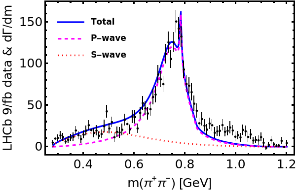
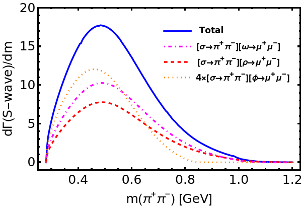
Figure 3: The prediction for the differential decay rate $d\Gamma/dm$ and LHCb data over the di-hadron invariant mass $m(\pi^{+}\pi^{-})\equiv\sqrt{p^{2}}$ [2, 3, 4]. (Left) The contributions from the $S$-wave (dotted red) and the $P$-wave (dashed magenta) add up to the full resonant contribution (solid blue). (Right) Components of the $S$-wave contribution: $\sigma\rho$ (dashed red), $\sigma\omega$ (dot-dashed magenta), and $\sigma\phi$ (dotted orange, multiplied by $4$ for an easier comparison).

We now discuss the features of the $d\Gamma/dq^{2}$ distribution. We fit the data of Refs. [2, 3, 4] in the region $q^{2}\geq m_{\rho}^{2}$, in order to avoid the many other resonances that we do not address in the present work, shown in Fig. 1. Fig. 4 displays the result of our fit, which achieves a good qualitative description of the data. Quantitatively, the fit does not perform well at the $\phi$ resonance, underestimating the branching ratio therein; the fit indicates that a broader width of the $\phi$ should be considered, i.e., the predicted values closer to $m_{\phi}$ tend to be overestimated, while peripheral values away from $m_{\phi}$ by $\Gamma^{0}_{\phi}=4.25~{}\text{MeV}$ [25] tend to be underestimated. Accordingly, we observe that a much better fit of the $d\Gamma/dq^{2}$ data is achieved when increasing the width of the $\phi$ by about 60%, namely, the $\chi^{2}_{min}$ drops significantly. This effect should be due to limited momentum resolution at LHCb (bin migration is found to be negligible in Ref. [5]), whose effect has not been “unfolded”, thus broadening the $\phi$ peak; efficiency variations, instead, are taken into account [82]. We fix the $\phi$ width to $\Gamma^{0}_{\phi}$ in our theoretical predictions, and to circumvent the later resolution issue we collect the four bins around the $\phi$ peak into a single bin.

From the global fit we find the following value for the overall normalization factor (intervals of about $3\sigma$ C.L. are provided in this section):

$$0.8\lesssim A_{1}(0)\,B_{\rho^{0}}\lesssim 1.2\,,$$ (85)

for the extraction of which we employ also information about the total branching fraction provided in Eq. (1). A value of $A_{1}(0)$ close to $0.6$ as in Ref. [84] implies $B_{\rho^{0}}$ of around $1.8$. For ratios of normalization factors (or “fudge factors”) we have:

$$0.8\lesssim B_{\phi}/B_{\rho^{0}} \lesssim 0.9\,,$$ (86)

$$0.9\lesssim B^{(S)}_{\omega}/B^{(S)}_{\rho^{0}} \lesssim 1.1\,,$$ (87)

$$0.05\lesssim B^{(S)}_{\phi}/B^{(S)}_{\rho^{0}} \lesssim 0.27\,.$$ (88)

The $\phi,\omega\to\mu^{+}\mu^{-}$ resonant branching ratios constrain precisely the parameters $B_{\phi}/B_{\rho^{0}}$ and $B^{(S)}_{\omega}/B^{(S)}_{\rho^{0}}$. The inclusion of $d\Gamma/dp^{2}$ data has an important impact in limiting the size of $B^{(S)}_{\phi}/B^{(S)}_{\rho^{0}}$, which reflects differently compared to the other two contributions $\sigma\omega$ and $\sigma\rho^{0}$, see the right panel of Fig. 3, due to the different available $p^{2}$ intervals as seen from Fig. 1. It is evident that an important deviation from naive factorization shows up in the extraction of $B^{(S)}_{\phi}/B^{(S)}_{\rho^{0}}$, which lies substantially away from $1$. It is interesting to point out that the contribution from $\sigma\phi$ also turns out to be suppressed in the amplitude analysis of $D^{0}\to K^{+}K^{-}\pi^{+}\pi^{-}$ by LHCb [31]. We also extract:

$$0.001\lesssim a_{\omega} \lesssim 0.005\,,$$ (89)

$$1.1\,\pi\lesssim \phi_{\omega} \lesssim 1.7\,\pi\,,$$ (90)

$$39~{}\text{GeV}\lesssim \frac{a_{S}(0)}{A_{1}(0)} \lesssim 62~{}\text{GeV}\,,$$ (91)

which compare relatively well with $a_{\omega}\simeq 0.006$, $\phi_{\omega}\simeq 0.9\,\pi$ and $a_{S}(0)/A_{1}(0)\simeq 24~{}\text{GeV}$ for the analogous semi-leptonic decay $D^{+}\to\pi^{+}\pi^{-}e^{+}\nu_{e}$ [26], see App. B for further discussion.

The fit is also used to extract the following range for the relative angle $\Delta_{1}=\delta_{\{\rho^{0}/\omega,\rho^{0}\}}-\delta_{\{\rho^{0}/\omega,\phi\}}$, see the left panel of Fig. 4:

$$0.5\,\pi\lesssim\Delta_{1}\lesssim 0.9\,\pi\,,$$ (92)

while $\Delta_{3}=\delta_{\{\sigma,\rho^{0}\}}-\delta_{\{\sigma,\phi\}}$ remains unconstrained, since the contribution from the $\sigma$ plays a less important role in the region between the $\rho^{0}$ and $\phi$ resonances with respect to the $P$-wave contribution. As it is clear from the left panel of Fig. 4, this strong phase has a huge impact in the latter inter-resonant region and the very-high energy region above the $\phi$ resonance, implying modulations of the predicted branching ratios by orders of magnitude in both cases. It is interesting to point out the possible correlation between the inter-resonant and the very-high energy regions due to the $\phi$ line-shape, e.g., a large suppression of the SM prediction in the very-high energy region (making then this region more sensitive to NP contributions) can be correlated to a relatively large branching ratio in the inter-resonant region; a similar effect is seen in Ref. [14]. In the right panel of Fig. 4, we illustrate the dependence of our prediction on the remaining strong-phase differences. As it has been discussed around Eq. (2.3), the contribution of the $\omega\to\ell^{+}\ell^{-}$ paired with the pion pair in a $P$-wave is suppressed; on the other hand, the $\omega\to\ell^{+}\ell^{-}$ can manifest when combined with the pion pair in the $S$-wave. We then find for $\Delta_{4}=\delta_{\{\sigma,\rho^{0}\}}-\delta_{\{\sigma,\omega\}}$:

$$0.2\,\pi\lesssim\Delta_{4}\lesssim 0.5\,\pi\,,$$ (93)

see the right panel of Fig. 4. It is rather difficult to provide interpretations to the extracted ranges of values for $\Delta_{1}$ and $\Delta_{4}$, or make comparisons to other processes; note that the $\rho^{0}$ and the $\omega$ or the $\phi$ are in different isospin irreducible representations, so that the dynamics involved in the rescattering processes with the second resonance (the $\rho^{0}/\omega$ in the case of $\Delta_{1}$, and the $\sigma$ in the case of $\Delta_{4}$) is expected to be substantially different.

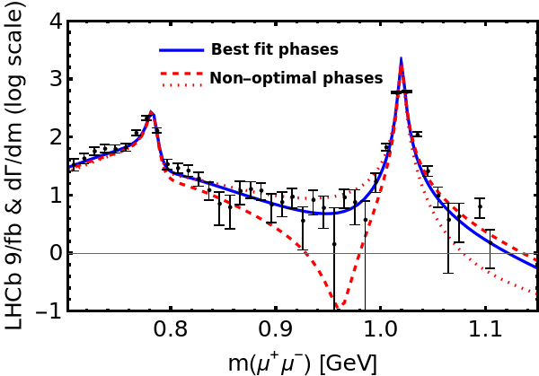
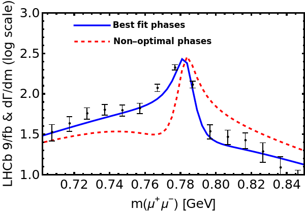
Figure 4: The differential decay rate $d\Gamma/dm$ and LHCb data over the di-lepton invariant mass $m(\mu^{+}\mu^{-})\equiv\sqrt{q^{2}}$ [2, 3, 4]. (Left) The dashed (dotted) red curve displaying “non-optimal phases” corresponds to the optimal $\Delta_{1}$ added with $\pi/2$ ($-3\pi/4$). (Right) The dashed red curve displaying “non-optimal phases” corresponds to the optimal $\Delta_{4}$ added with $5\pi/4$.

$q^{2}$-bin	$\Gamma^{r}$ (SM)	$\frac{\Gamma_{\sigma}^{r}}{\Gamma^{r}}$ (%)	$\int\langle I_{2}\rangle_{+}^{r}\times 100$	$\frac{\int\langle I_{2}\rangle_{+,\sigma}^{r}}{\int\langle I_{2}\rangle_{+}^{r}}$ (%)	$\int\langle I_{3}\rangle_{+}^{r}\times 100$	$\int\langle I_{4}\rangle_{-}^{r}\times 100$
$r^{(\rho:{\rm sup})}$	$[0.64,0.87]$	$[23,43]$	$[-16,-8.5]$	$[59,78]$	$[-7.2,-4.7]$	$[8.3,13]$
$r^{(\phi:{\rm inf})}$	$[1.6,1.9]$	$[0.3,8]$	$[-11,-6.2]$	$[3,45]$	$[-30,-26]$	$[36,41]$
$r^{(\phi:{\rm sup})}$	$[1.2,1.3]$	$[0.8,10]$	$[-8.7,-4.3]$	$[8,53]$	$[-22,-19]$	$[26,29]$

Table 2: SM predictions for the non-vanishing observables which only receive $P$-wave contributions ($\int\langle I_{3}\rangle_{+}^{r}\,,\;\int\langle I_{4}\rangle_{-}^{r}$), and where the effect of the $S$-wave is additive (i.e., $\Gamma^{r}=\Gamma^{r}_{\rho^{0}/\omega}+\Gamma^{r}_{\sigma}$ and $\int\langle I_{2}\rangle_{+}^{r}=\int\langle I_{2}\rangle_{+,\rho^{0}/\omega}^{r}+\int\langle I_{2}\rangle_{+,\sigma}^{r}$); a subscript $\sigma$ indicates that only the $S$-wave is kept. The relation $\Gamma^{r}=2\left(\int\langle I_{1}\rangle_{+}^{r}-\int\langle I_{2}\rangle_{+}^{r}/3\right)$ holds true. For comparison with LHCb [2, 3, 4], $\langle S_{2}\rangle^{r}=\int\langle I_{2}\rangle_{+}^{r}/\Gamma^{r}$, $\langle S_{3}\rangle^{r}=\int\langle I_{3}\rangle_{+}^{r}/\Gamma^{r}$, and $\langle S_{4}\rangle^{r}=\int\langle I_{4}\rangle_{-}^{r}/\Gamma^{r}$. Relevant definitions can be found in Sec. 3, see in particular Eqs. (81) and (82). The decay rate and the $I_{i}$’s both need to be multiplied by a common constant factor, $|C_{2}\lambda_{d}eG_{F}/\sqrt{2}|^{2}\frac{e^{2}}{m_{D}}\times 10^{-4}=2.4\times 10^{-19}$, with $G_{F}$, $m_{D}$ and $\Gamma^{r}$ in GeV.

We now discuss our predictions and the available data for the angular observables. Following LHCb [2, 3, 4], we define the ranges:

$$r^{(\rho:{\rm sup})} \equiv \;\;[0.78^{2},0.95^{2}]\;\text{GeV}^{2}\,,$$ (94)

$$r^{(\phi:{\rm inf})} \equiv \;\;[0.95^{2},1.02^{2}]\;\text{GeV}^{2}\,,$$

$$r^{(\phi:{\rm sup})} \equiv \;\;\;[1.02^{2},1.1^{2}]\;\text{GeV}^{2}\,.$$

Since we focus on the high-energy window of Fig. 1, we will discuss predictions for these three bins, while LHCb also provides results for the bins $[0.212^{2},0.525^{2}]\;\text{GeV}^{2}$ and $[0.565^{2},0.78^{2}]\;\text{GeV}^{2}$; the bin $[0.565^{2},0.78^{2}]\;\text{GeV}^{2}$, however, is also used for determining the total branching ratio distribution as a function of $p^{2}$ (the branching ratio outside these four $q^{2}$-bins is highly suppressed). In Tab. 2 we present predicted values for those observables that do not vanish in the SM, in particular in the presence of the $S$-wave, in cases where it does not interfere with the $P$-wave. As seen in this table, the $\sigma$ provides significant contributions, as large as $10-40$% in the binned branching ratios. This fraction is even larger in the case of $\int\langle I_{2}\rangle_{+,\sigma}^{r}$, which contributes to the binned branching ratio $\Gamma^{r}=2\left(\int\langle I_{1}\rangle_{+}^{r}-\int\langle I_{2}\rangle_{+}^{r}/3\right)$, reaching up to about $50-80$% of $\int\langle I_{2}\rangle_{+}^{r}$. The dominance of the $S$-wave in this observable can be attributed to a suppression of the $P$-wave contribution, due to a cancellation among the transversity form factors as seen from Eq. (72) (also manifesting in the case of $\int\langle I_{3}\rangle_{+}^{r}$), which on the other hand are added constructively in the case of $\langle I_{1}\rangle_{+}^{r}$, cf. Eq. (71). In performing a comparison of our predictions to LHCb data of the observables $\langle S_{2}\rangle^{r}$, $\langle S_{3}\rangle^{r}$, and $\langle S_{4}\rangle^{r}$ in the three bins $r^{(\rho:{\rm sup})}$, $r^{(\phi:{\rm inf})}$, and $r^{(\phi:{\rm sup})}$ we obtain a $p$-value of $\mathcal{O}(10)\%$.

As we have seen, our predictions for the angular observables $\langle S_{7}\rangle^{r}$, $\langle S_{8}\rangle^{r}$, and $\langle S_{9}\rangle^{r}$ (approximately) vanish, even in presence of NP; we find however a poor comparison with the hypothesis that they are all zero in the five bins of Eq. (94), $\chi^{2}/N_{\rm d.o.f.}\simeq 2.4$ (where $N_{\rm d.o.f.}\simeq 15$), or a $p$-value of $0.2\%$, due to $\langle S_{9}\rangle^{r}$. This may indicate a missing description of the relative strong phases among the transversity form factors $\mathcal{F}_{P}$, $\mathcal{F}_{\|}$, and $\mathcal{F}_{\perp}$. (Including in this latter test the $\langle S_{5}\rangle^{r}$ and $\langle S_{6}\rangle^{r}$ observables, which also vanish in the SM, we get $\chi^{2}/N_{\rm d.o.f.}\simeq 2.0$ (where $N_{\rm d.o.f.}\simeq 25$), or a $p$-value of $0.2\%$, which is small also as a consequence of including $\langle S_{9}\rangle^{r}$.) The violation of CP is surely exciting in the context of charm physics, where a sizable level of CP violation has been recently measured by LHCb [85, 86] in hadronic two-body charm-meson decays, see Ref. [87] for a theoretical discussion. On the other hand, the CP asymmetries in rare charm-meson decays are consistent with zero, since in this case we find that $p$-value $=84\%$. Note that statistical correlations among bins and across observables are provided by the LHCb analysis; they are small, but have been included. Systematic uncertainties are smaller than statistical uncertainties, and are fully correlated (we use the techniques discussed in Ref. [88] to combine both categories of uncertainties in presence of correlations).

In Tab. 3 we provide the values for non-vanishing angular observables that probe the interference of the $S$- and $P$-waves. These observables depend on the relative phase $\Delta_{SP}=\delta_{\{\sigma,\rho^{0}\}}-\delta_{\{\rho^{0}/\omega,\rho^{0}\}}$ between the $S$- and $P$-waves. None of the experimentally provided observables from Refs. [2, 3, 4] is sensitive to this phase, hence it is left as a free parameter. A future experimental analysis would probe this phase difference, possibly in combination with the differential distribution over the di-hadron angle, as discussed later in this section. As seen in the table, some sizable values are found, typically smaller but of similar order compared to the ones provided in Tab. 2 that are insensitive to the $S$-wave.

$q^{2}$-bin	$\int\langle I_{2}\rangle_{-}^{r}\times 100$
$r^{(\rho:{\rm sup})}$	$[-6.6,-0.8]\,c_{SP}+[-2.3,-1.1]\,s_{SP}$
$r^{(\phi:{\rm inf})}$	$[-7.7,6.1]\,c_{SP}+[-5.3,8.2]\,s_{SP}$
$r^{(\phi:{\rm sup})}$	$[-7.1,3.0]\,c_{SP}+[-5.0,5.4]\,s_{SP}$
$q^{2}$-bin	$\int\langle I_{4}\rangle_{+}^{r}\times 100$
$r^{(\rho:{\rm sup})}$	$[0.8,5.9]\,c_{SP}+[0.4,1.6]\,s_{SP}$
$r^{(\phi:{\rm inf})}$	$[-6.7,8.3]\,c_{SP}+[-8.6,5.4]\,s_{SP}$
$r^{(\phi:{\rm sup})}$	$[-3.1,7.6]\,c_{SP}+[-5.9,5.5]\,s_{SP}$
$q^{2}$-bin	$\int\langle I_{8}\rangle_{+}^{r}\times 100$
$r^{(\rho:{\rm sup})}$	$[-3.0,-0.2]\,c_{SP}+[-0.4,0.4]\,s_{SP}$
$r^{(\phi:{\rm inf})}$	$[-4.6,4.5]\,c_{SP}+[-3.4,4.0]\,s_{SP}$
$r^{(\phi:{\rm sup})}$	$[-2.6,3.3]\,c_{SP}+[-1.7,3.3]\,s_{SP}$

Table 3: SM predictions for the non-vanishing angular observables that probe the interference between the $S$- and $P$-waves. The parameters appearing stand for $c_{SP}\equiv\cos(\Delta_{SP})$ and $s_{SP}\equiv\sin(\Delta_{SP})$. The relation $\int\langle I_{1}\rangle_{-}^{r}=-\int\langle I_{2}\rangle_{-}^{r}$ holds true. Relevant definitions can be found in Sec. 3, see in particular Eqs. (81) and (82). The same overall multiplicative factor shown in the caption of Tab. 2 applies.

Finally, as announced in the introduction, the $S$-wave can produce distinguished signatures in the differential branching ratio as a function of the angular variables describing the topology of the rare decay. To illustrate this point, consider:

$$\frac{d\Gamma}{d\cos\theta_{\pi}}=\langle I_{1}\rangle_{+,\rho^{0}/\omega}^{r}+\langle I_{2}\rangle_{+,\rho^{0}/\omega}^{r}\,(1-4\cos^{2}\theta_{\pi})-\frac{4}{3}\langle I_{2}\rangle_{+,\sigma}^{r}-\frac{8}{3}\langle I_{2}\rangle_{-}^{r}\,\cos\theta_{\pi}\,,$$ (95)

after integration over the $q^{2}$-bin $r$, where the contributions from the $S$- and $P$-waves alone are indicated in subscript (here, the $\sigma$ and $\rho^{0}/\omega$ resonances, respectively), and the last term in the right-hand side probes their interference. As seen in Fig. 5, the presence of the $S$-wave can produce an asymmetry of the distribution with respect to $\cos\theta_{\pi}=0$. This provides motivation for binned measurements of the branching ratio as a function of the angular variables.

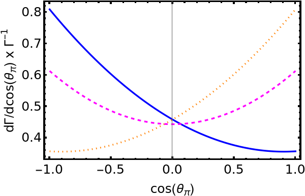
Figure 5: The differential decay rate, after integration of di-lepton energies over the range $r^{(\rho:{\rm sup})}\cup r^{(\phi:{\rm inf})}\cup r^{(\phi:{\rm sup})}=[0.78^{2},1.1^{2}]\;\text{GeV}^{2}$, as a function of $\cos(\theta_{\pi})$. In dashed magenta the observable is shown in the absence of the $S$-wave contribution (rescaled such that $\int^{1}_{-1}d\cos(\theta_{\pi})d\Gamma/d\cos(\theta_{\pi})/\Gamma=1$). The solid blue and dotted orange lines correspond to extreme cases reached for certain values of the phase difference $\Delta_{SP}$ between the $S$- and $P$-waves that maximize their interference. As it is clear from the figure, the interference of the $S$- and $P$-waves can generate a distinguished asymmetry.

4.2 Semi-leptonic operators from generic NP

We want to know the impact of having dimension-6 operators that can mediate the transition $c\to u\ell^{+}\ell^{-}$ at the quark level due to interactions mediated by heavy NP. We focus on vector and axial-vector structures. Present bounds @ 95% C.L. are [19]:

$$|\tilde{C}^{\rm NP}_{9}|,|\tilde{C}^{\prime}_{9}|<1.2\,,\quad|\tilde{C}_{10}^{(^{\prime})}|<0.43\,,$$ (96)

where $|\tilde{C}|=|V_{ub}V_{cb}^{\ast}C|$, and the former bound results from the $D^{+}\to\pi^{+}\mu^{+}\mu^{-}$ branching ratio [89], while the second from the $D^{0}\to\mu^{+}\mu^{-}$ branching ratio [90]. Slightly better bounds are found from collider searches for contact interactions manifesting in $pp\to\mu^{+}\mu^{-}$ [91]. In view of these constraints, it is justified to assume that NP does not affect the previous discussion about the differential branching ratio as a function of the invariant masses of pion and lepton pairs. However, NP could still affect the differential branching ratio in the low and very-high di-lepton invariant mass regions [14]. It can also affect distinct angular observables as we now discuss.

As seen from the expressions provided in Sec. 3, there are distinct observables that depend on these Wilson coefficients. In Tab. 4 we provide predictions for those observables sensitive to the SM-NP interference in presence of a non-vanishing $C_{10}$ Wilson coefficient (its SM value is very suppressed, as discussed around Eq. (2)). The cases $\braket{I_{5}}_{-}$ and $\braket{I_{6}}_{+}$ are sensitive to the SM-NP interference through the $P$-wave, while $\braket{I_{7}}_{-}$ approximately vanishes. These observables, which isolate the NP interference with the SM $P$-wave, are given as functions of the phase difference

$$\Delta_{\rho{\rm NP}}\equiv\delta_{\{\rho^{0}/\omega,\rho^{0}\}}-\delta_{Q_{10}}\,,$$ (97)

where $\delta_{Q_{10}}$ allows for a possible strong phase when considering insertions of the $Q_{10}$ operator (beyond the one from the pion pair line-shape). Predictions are shown in Tab. 3.

On the other hand, the cases $\braket{I_{5}}_{+}$ and $\braket{I_{7}}_{+}$ are sensitive to the SM-NP interference in the presence of the $S$-wave. These observables depend on the above phase $\Delta_{\rho{\rm NP}}$ together with $\Delta_{SP}$. The latter phase difference can be probed based on the observables whose predictions are given in Tab. 3, and the observable shown in Fig. 5. Given the dependence on both phase differences, we do not give explicitly the expressions for the related angular observables. By varying these phases, we stress that we find values of the angular observables comparable to the ones found for the analogous $P$-wave null tests in Tab. 3.

Given the bounds shown above in Eq. (96), detecting NP requires sub-percentage precision in the measurement of the angular observables. Having reached such precision, some bins of the angular observables sensitive to the $S$-wave provide additional complementary information to favor or disfavor an observation of a possible NP manifestation based on the $P$-wave cases. In the future, a global fit could extract all relevant phases, together with possible NP contributions. It is possible that a clever strategy could circumvent the need to extract at least some of the strong phases affecting the angular observables.

$q^{2}$-bin	$\int\langle I_{5}\rangle_{-}^{r}\times 100$
$r^{(\rho:{\rm sup})}$	$[0.49,0.83]\,c_{\rho{\rm NP}}+[-1.5,-1.3]\,s_{\rho{\rm NP}}$
$r^{(\phi:{\rm inf})}$	$[-0.36,0.50]\,c_{\rho{\rm NP}}+[-0.83,-0.60]\,s_{\rho{\rm NP}}$
$r^{(\phi:{\rm sup})}$	$[0.31,0.66]\,c_{\rho{\rm NP}}+[-0.09,0.49]\,s_{\rho{\rm NP}}$
$q^{2}$-bin	$\int\langle I_{6}\rangle_{+}^{r}\times 100$
$r^{(\rho:{\rm sup})}$	$[0.7,1.2]\,c_{\rho{\rm NP}}+[-2.1,-1.7]\,s_{\rho{\rm NP}}$
$r^{(\phi:{\rm inf})}$	$[-0.57,0.78]\,c_{\rho{\rm NP}}+[-1.3,-1.0]\,s_{\rho{\rm NP}}$
$r^{(\phi:{\rm sup})}$	$[0.5,1.1]\,c_{\rho{\rm NP}}+[-0.14,0.78]\,s_{\rho{\rm NP}}$

Table 4: Observables that vanish in the SM, arising from the interference of the $P$-wave and NP, here calculated for $C_{9}^{\prime}=C_{10}^{\prime}=C_{9}^{\rm NP}=0$ and non-zero $C_{10}$. The parameters appearing stand for $c_{\rho{\rm NP}}=\cos(\Delta_{\rho{\rm NP}})$ and $s_{\rho{\rm NP}}=\sin(\Delta_{\rho{\rm NP}})$. The other $P$-wave dependent observable $\braket{I_{7}}_{-}$ approximately vanishes. The NP does not interfere with the SM in the decay rate, and can thus be neglected. Relevant definitions can be found in Sec. 3, see in particular Eqs. (81) and (82). The same overall multiplicative factor shown in the caption of Tab. 2 applies; additionally, there is an extra $\tilde{C}_{10}$ that multiplies the observables.

5 Conclusions

Recent experimental data by LHCb open up the opportunity for precision physics with rare charm-meson decays, a task that can be assisted by complementary information coming from experiments such as BESIII, and by Belle II in different rare decay modes. For this sake, better theoretical predictions are needed, in particular the description of resonances, without which it will not be possible to disentangle non-SM contributions from the large SM background; better theoretical predictions of the SM are also needed in order to describe possible interference terms with non-SM contributions. We employ a factorization model for the inclusion of intermediate hadronic states contributing to $D^{0}\to\pi^{+}\pi^{-}\ell^{+}\ell^{-}$ in the SM, and discuss in details different contributing topologies. Within this framework, the novelty of this work concerns the inclusion of the lightest scalar isoscalar state, which is a very broad resonance manifesting in long-distance pion pair interactions and impacts a large portion of the allowed phase space, see Fig. 1. We highlight that $D^{0}\to\pi^{+}\pi^{-}\ell^{+}\ell^{-}$ data already show the clear emergence of such $S$-wave effects, see Fig. 3. Moreover, current data also allows the study of the strong phases among intermediate resonances, see Fig. 4.

The decay $D^{0}\to\pi^{+}\pi^{-}\ell^{+}\ell^{-}$ offers the possibility to define a rich set of angular observables. We then discuss angular observables that are sensitive to both the $S$- and $P$-waves. Predictions are given in Tabs. 2 and 3. We have been able to understand the overall pattern of the measured angular observables $\langle S_{i}\rangle^{r}$, $i=2,\ldots,8$, in distinct $q^{2}$-bins $r$. To further improve our understanding of SM contributions, we suggest experimentalists measure additional observables to further test and better characterise the contributions of the $S$-wave, such as following the strategy illustrated in Fig. 5.

Such additional observables have also an interest other than improving non-perturbative aspects of the SM description. Indeed, the search for NP consists of one of the main motivations for looking into this category of rare decay processes. If any deviation is seen while performing a null test of the SM, a comprehensive analysis will be needed to verify and characterize it. We emphasize the potential for complementary tests of NP via its interference with the SM in the presence of the $S$-wave, which provide distinct null tests of the SM, as seen from Tab. 4.

In order to improve the description of the differential branching ratio, in particular the one as a function of the pion pair invariant mass, future theoretical directions include incorporating other $S$- and $P$-wave resonances and the $D$-wave following a similar theoretical framework, isospin-two contributions, and the addition of cascade decays. More studies will be needed to understand the set of angular observables measured by LHCb in more details, since with our simple factorization model some tension appears in the description of the angular observable $\langle S_{9}\rangle^{r}$. It would also be interesting to extend our analysis to include $D^{0}\to K^{+}K^{-}\mu^{+}\mu^{-}$ and radiative decay modes.

Acknowledgements

We thank Fernando Abudinén, Damir Becirevic, Thomas Blake, Luka Leskovec, Lei Li, Serena Maccolini, Dominik Mitzel, Juan Nieves, Eulogio Oset, Tommaso Pajero, Antonio Pich, Luka Santelj and Shulei Zhang for helpful communication. E. S. is grateful to Gudrun Hiller and the rest of the participants for helpful discussions during the “First CharmInDor mini workshop”.

This work has been supported by MCIN/AEI/10.13039/501100011033, grants PID2020-114473GB-I00 and PRE2018-085325, and by Generalitat Valenciana, grant PROMETEO/2021/071. This project has received funding from the European Union’s Horizon 2020 research and innovation programme under the Marie Sklodowska-Curie grant agreement No 101031558. S. F. acknowledges the financial support from the Slovenian Research Agency (research core funding No. P1-0035). L. V. S. is grateful for the hospitality of the Jožef Stefan Institute and the CERN-TH group where part of this research was executed.

Appendix A Hadronic inputs

A.1 Decay constants

We have from Ref. [72]:

$$\langle\phi|\bar{s}\gamma_{\mu}s|0\rangle=\epsilon_{\mu}^{\ast}m_{\phi}f_{\phi}\,,\;\;\hat{c}^{q}_{\omega}\langle\omega|\bar{q}\gamma_{\mu}q|0\rangle=\epsilon_{\mu}^{\ast}m_{\omega}f^{(q)}_{\omega}\,,\;\;\hat{c}^{q}_{\rho^{0}}\langle\rho^{0}|\bar{q}\gamma_{\mu}q|0\rangle=\epsilon_{\mu}^{\ast}m_{\rho^{0}}f^{(q)}_{\rho^{0}}\,,$$ (98)

with $\hat{c}^{u}_{\rho^{0}}=-\hat{c}^{d}_{\rho^{0}}=\hat{c}^{u}_{\omega}=\hat{c}^{d}_{\omega}=\sqrt{2}$. We consider a single decay constant for both matrix elements of $u$- and $d$-quark bilinears, i.e., $f^{(q)}_{\omega}\to f_{\omega}$ and $f^{(q)}_{\rho^{0}}\to f_{\rho^{0}}$, which is good enough for our purposes. The decay constants are then:

$$f_{\rho^{0}}=216(3)~{}\text{MeV}\,,\quad f_{\omega}=197(8)~{}\text{MeV}\,,\quad f_{\phi}=233(4)~{}\text{MeV}\,.$$ (99)

(Mixing effects $\omega-\rho^{0}$ and $\omega-\phi$ have been included, but are small.)

A.2 Form factors

For the $D\to\mathcal{V}$ form factors, for both $\mathcal{V}=\rho^{0},\omega$, we use the nearest pole approximation introduced in Ref. [71], which has the general form

$$F(q^{2})=F(0)/\left(1-\frac{q^{2}}{m_{\text{pole}}^{2}}\right)\,.$$ (100)

The pole masses implemented are $2.42$ GeV ($J^{P}=1^{+}$) for $F=A_{1}$ and $A_{2}$, and $2.01$ GeV ($J^{P}=1^{-}$) for $F=V$. We define:

$$r_{V}=\frac{V(0)}{A_{1}(0)}\,,\quad r_{2}=\frac{A_{2}(0)}{A_{1}(0)}\,,$$ (101)

for which Ref. [26] gives $r_{V}=1.695\pm 0.083\pm 0.051$ and $r_{2}=0.845\pm 0.056\pm 0.039$ (with a correlation of $\rho_{r_{V},r_{2}}=-0.206$), where the first (second) uncertainty is statistical (respectively, systematic).

A.3 Line shapes

We reproduce the line shape of $f_{0}(500)$ [23]:

$$\mathcal{A}_{S}(s)=\left[M^{2}-s-g_{1}^{2}(s)\frac{s-s_{A}}{M^{2}-s_{A}}z(s)-i\,M\,\Gamma_{tot}(s)\right]^{-1}\,,$$ (102)

$$\Gamma_{tot}(s)=\sum^{4}_{i=1}\Gamma_{i}(s)\,,$$ (103)

$$M\,\Gamma_{1}(s)=g_{1}^{2}(s)\frac{s-s_{A}}{M^{2}-s_{A}}\rho_{1}(s)\,,$$ (104)

$$\rho_{1}(s)=\sqrt{1-4\,m_{\pi}^{2}/s}\,,$$ (105)

$$g_{1}^{2}(s)=M\,\left(b_{1}+b_{2}\,s\right)\,\exp[-(s-M^{2})/A]\,,$$ (106)

$$z(s)=j_{1}(s)-j_{1}(M^{2})\,,$$ (107)

$$j_{1}(s)=\frac{1}{\pi}\left[2+\rho_{1}(s)\,\log\left(\frac{1-\rho_{1}(s)}{1+\rho_{1}(s)}\right)\right]\,,$$ (108)

$$M\,\Gamma_{2}(s)=0.6\,g_{1}^{2}(s)\,(s/M^{2})$$ (109)

$$\qquad\;\;\;\times\exp\left[-\alpha(s-4\,m_{K}^{2})\Theta(s-4\,m_{K}^{2})-\alpha^{\prime}(4\,m_{K}^{2}-s)\Theta(4\,m_{K}^{2}-s)\right]\rho_{2}(s)\,,$$

$$\rho_{2}(s)=\sqrt{1-4\,m_{K}^{2}/s}\,\Theta(s-4\,m_{K}^{2})+i\,\sqrt{4\,m_{K}^{2}/s-1}\,\Theta(4\,m_{K}^{2}-s)\,,$$ (110)

$$M\,\Gamma_{3}(s)=0.2\,g_{1}^{2}(s)\,(s/M^{2})$$ (111)

$$\qquad\;\;\;\times\exp\left[-\alpha(s-4\,m_{\eta}^{2})\Theta(s-4\,m_{\eta}^{2})-\alpha^{\prime}(4\,m_{\eta}^{2}-s)\Theta(4\,m_{\eta}^{2}-s)\right]\rho_{3}(s)\,,$$

$$\rho_{3}(s)=\sqrt{1-4\,m_{\eta}^{2}/s}\,\Theta(s-4\,m_{\eta}^{2})+i\,\sqrt{4\,m_{\eta}^{2}/s-1}\,\Theta(4\,m_{\eta}^{2}-s)\,,$$ (112)

$$M\,\Gamma_{4}(s)=M\,g_{4\pi}\,\rho_{4\pi}(s)/\rho_{4\pi}(M^{2})\,\Theta(s-16\,m_{\pi}^{2})\,,$$ (113)

$$\rho_{4\pi}(s)=1.0/\left[1+\exp(7.082-2.845\,s/\text{GeV}^{2})\right]\,,$$ (114)

$$s_{A}\simeq 0.41\,m_{\pi}^{2}\,,\quad\alpha=1.3\,\text{GeV}^{-2}\,,\quad\alpha^{\prime}=2.1\,\text{GeV}^{-2}\,,$$ (115)

and (solution (iii) of Ref. [23]): $M=0.953$ GeV, $b_{1}=1.302$ GeV, $b_{2}=0.340$/GeV, $A=2.426$ GeV², $g_{4\pi}=0.011$ GeV.

For the line shape of the $\rho(770)^{0}$ in $\pi^{+}\pi^{-}$ decays, we adopt the Gounaris-Sakurai parameterization [74]:

$$P_{\rho^{0}}(s)=m_{\rho^{0}}^{2}-s+f(s)-i\,m_{\rho^{0}}\,\Gamma_{\rho^{0}}(s)\,,$$ (116)

$$f(s)=\Gamma_{\rho^{0}}^{0}\frac{m_{\rho^{0}}^{2}}{k_{\rho^{0}}^{3}}\left\{k(s)^{2}\left[h(s)-h(m_{\rho^{0}}^{2})\right]+k_{\rho^{0}}^{2}\,(m_{\rho^{0}}^{2}-s)\,h^{\prime}(m_{\rho^{0}}^{2})\right\}\,,$$ (117)

$$\Gamma_{\rho^{0}}(s)=\Gamma_{\rho^{0}}^{0}\left(\frac{k(s)}{k_{\rho^{0}}}\right)^{3}\frac{m_{\rho^{0}}}{\sqrt{s}}\,,$$ (118)

$$h(s)=\frac{2}{\pi}\frac{k(s)}{\sqrt{s}}\log\left(\frac{\sqrt{s}+2\,k(s)}{2\,m_{\pi}}\right)\,,$$ (119)

$$k(s)=\left(\frac{1}{4}s-m_{\pi}^{2}\right)^{1/2}\,,\quad k_{\rho^{0}}=\left(\frac{1}{4}m_{\rho^{0}}^{2}-m_{\pi}^{2}\right)^{1/2}\,.$$ (120)

We also have [26, 92, 93]:

$$\text{RBW}_{\omega}(s)=\frac{s}{m_{\omega}^{2}-s-i\,m_{\omega}\,\Gamma_{\omega}^{0}}\,,$$ (121)

and

$$F_{BW}(p^{2})=B(p^{*})/B(p_{0}^{*})\,,$$ (122)

$$B(p^{\ast})=\frac{1}{\sqrt{1+r^{2}_{BW}\,(p^{\ast})^{2}}}\,.$$ (123)

The value of $r_{BW}$ is taken to be $3.0/$GeV (i.e., the inverse of a non-perturbative scale) [26]. The function $p^{\ast}(p^{2})=\sqrt{\lambda(p^{2},m_{\pi}^{2},m_{\pi}^{2})}/(2\sqrt{p^{2}})$, and $p^{\ast}_{0}=p^{\ast}(m^{2}_{\rho^{0}})$. The $\phi$ and the $\omega$ line-shapes, when the latter decays to the lepton pair, are just Breit-Wigner line-shapes:

$$P_{\phi}(s)=m_{\phi}^{2}-s-i\,m_{\phi}\,\Gamma_{\phi}^{0}\,,\quad P_{\omega}(s)=m_{\omega}^{2}-s-i\,m_{\omega}\,\Gamma_{\omega}^{0}\,,$$ (124)

The masses and widths are [25]:

$$m_{\rho^{0}}=775.3~{}\text{MeV}\,,\;\;\Gamma^{0}_{\rho^{0}}=147.4~{}\text{MeV}\,,$$ (125)

$$m_{\omega}=782.7~{}\text{MeV}\,,\;\;\Gamma^{0}_{\omega}=8.7~{}\text{MeV}\,,$$ (126)

$$m_{\phi}=1019.46~{}\text{MeV}\,,\;\;\Gamma^{0}_{\phi}=4.25~{}\text{MeV}\,.$$ (127)

Appendix B Further comments on semi-leptonic decays

To reproduce the values in Table I of [26] relative to $D^{+}$ decays, we find: $a_{S}(0)=8.6\pm 0.4$ GeV, $a_{\omega}=0.006\pm 0.001$, and $A_{1}(0)=0.36$. The strong phases extracted in their analysis are $\phi_{S}=3.4044\pm 0.0738$, which is somewhat the analogous of $\Delta_{SP}$ defined in the main text, and $\phi_{\omega}=2.93\pm 0.17$ [93]; this latter angle is consistent with $\pi$ from the isospin decomposition of the $(\bar{d}d)_{V}$ current, that generates the states $\rho^{0}$ and $\omega$. Instead, we employ in this work the values extracted from a fit to the data of Refs. [2, 3, 4], see Fig. 3. In doing so, we obtain the values quoted in Eq. (89), which in the case of $a_{S}(0)/A_{1}(0)$ is about 2 times larger than the value shown above. The comparison, however, is not straightforward, since the $\sigma$ contributes in three dynamical ways when combined with the $\rho^{0},\omega,\phi$ that lead to the lepton pair. Note that the resonance that decays into pion pairs originates from both $u$- (in the W-type topology) and $d$-quark pairs (in the J-type topology), which differs from the situation depicted above for $\phi_{\omega}$. Likely, the extraction of the phase $\phi_{\omega}$ from data is contaminated by the presence of further resonances discussed in the main text that we do not include in our analysis, and the presence of further intermediate hadrons (i.e., vector mesons that lead to the lepton pair) in the full charm-meson decay process.

(For comparison with Ref. [27], there is an overall normalization factor, adapted for the line shape in use here:

$$\alpha_{GS}=\sqrt{\frac{3\,\pi\,\mathcal{B}_{\rho^{0}}}{p^{\ast}_{0}\,\Gamma_{\rho^{0}}^{0}}}\frac{\Gamma_{\rho^{0}}^{0}}{m_{\rho^{0}}}\,,\quad\mathcal{B}_{\rho^{0}}=1\,.)$$ (128)

References

- [1] S. L. Glashow, J. Iliopoulos, and L. Maiani. Weak Interactions with Lepton-Hadron Symmetry. Phys. Rev. D, 2:1285–1292, 1970. doi:10.1103/PhysRevD.2.1285.
- [2] Roel Aaij et al. Angular Analysis of and Decays and Search for Violation. Phys. Rev. Lett., 128(22):221801, 2022. arXiv:2111.03327, doi:10.1103/PhysRevLett.128.221801.
- [3] https://journals.aps.org/prl/supplemental/10.1103/PhysRevLett.128.221801/LHCb-PAPER-2021-035-supplemental.pdf (LHCb supplementary material).
- [4] https://lhcbproject.web.cern.ch/Publications/LHCbProjectPublic/LHCb-PAPER-2021-035.html (LHCb supplementary material).
- [5] R Aaij et al. Search for the decay . Phys. Lett. B, 728:234–243, 2014. arXiv:1310.2535, doi:10.1016/j.physletb.2013.11.053.
- [6] Roel Aaij et al. Observation of meson decays to and final states. Phys. Rev. Lett., 119(18):181805, 2017. arXiv:1707.08377, doi:10.1103/PhysRevLett.119.181805.
- [7] Roel Aaij et al. Measurement of Angular and CP Asymmetries in and decays. Phys. Rev. Lett., 121(9):091801, 2018. arXiv:1806.10793, doi:10.1103/PhysRevLett.121.091801.
- [8] https://lhcbproject.web.cern.ch/Publications/LHCbProjectPublic/LHCb-PAPER-2018-020.html (LHCb supplementary material). Note in particular relative efficiencies in as a function of , , , , and ; the latter is high for the low- region.
- [9] S. Fajfer, Sasa Prelovsek, and P. Singer. Resonant and nonresonant contributions to the weak D — V lepton+ lepton- decays. Phys. Rev. D, 58:094038, 1998. arXiv:hep-ph/9805461, doi:10.1103/PhysRevD.58.094038.
- [10] Gustavo Burdman, Eugene Golowich, JoAnne L. Hewett, and Sandip Pakvasa. Rare charm decays in the standard model and beyond. Phys. Rev. D, 66:014009, 2002. arXiv:hep-ph/0112235, doi:10.1103/PhysRevD.66.014009.
- [11] Svjetlana Fajfer and Sasa Prelovsek. Effects of littlest Higgs model in rare D meson decays. Phys. Rev. D, 73:054026, 2006. arXiv:hep-ph/0511048, doi:10.1103/PhysRevD.73.054026.
- [12] Ikaros I. Bigi and Ayan Paul. On CP Asymmetries in Two-, Three- and Four-Body D Decays. JHEP, 03:021, 2012. arXiv:1110.2862, doi:10.1007/JHEP03(2012)021.
- [13] Luigi Cappiello, Oscar Cata, and Giancarlo D’Ambrosio. Standard Model prediction and new physics tests for . JHEP, 04:135, 2013. arXiv:1209.4235, doi:10.1007/JHEP04(2013)135.
- [14] Stefan De Boer and Gudrun Hiller. Null tests from angular distributions in , decays on and off peak. Phys. Rev. D, 98(3):035041, 2018. arXiv:1805.08516, doi:10.1103/PhysRevD.98.035041.
- [15] Thorsten Feldmann, Bastian Müller, and Dirk Seidel. decays in the QCD factorization approach. JHEP, 08:105, 2017. arXiv:1705.05891, doi:10.1007/JHEP08(2017)105.
- [16] Aoife Bharucha, Diogo Boito, and Cédric Méaux. Disentangling QCD and new physics in . JHEP, 04:158, 2021. arXiv:2011.12856, doi:10.1007/JHEP04(2021)158.
- [17] Ayan Paul, Ikaros I. Bigi, and Stefan Recksiegel. On within the Standard Model and Frameworks like the Littlest Higgs Model with T Parity. Phys. Rev. D, 83:114006, 2011. arXiv:1101.6053, doi:10.1103/PhysRevD.83.114006.
- [18] Stefan de Boer and Gudrun Hiller. Flavor and new physics opportunities with rare charm decays into leptons. Phys. Rev. D, 93(7):074001, 2016. arXiv:1510.00311, doi:10.1103/PhysRevD.93.074001.
- [19] Svjetlana Fajfer and Nejc Košnik. Prospects of discovering new physics in rare charm decays. Eur. Phys. J. C, 75(12):567, 2015. arXiv:1510.00965, doi:10.1140/epjc/s10052-015-3801-2.
- [20] Rigo Bause, Marcel Golz, Gudrun Hiller, and Andrey Tayduganov. The new physics reach of null tests with and decays. Eur. Phys. J. C, 80(1):65, 2020. [Erratum: Eur.Phys.J.C 81, 219 (2021)]. arXiv:1909.11108, doi:10.1140/epjc/s10052-020-7621-7.
- [21] Marxil Sánchez, Genaro Toledo, and I. Heredia De La Cruz. Taming the long distance effects in the decay. Phys. Rev. D, 106(7):073002, 2022. doi:10.1103/PhysRevD.106.073002.
- [22] Hector Gisbert, Marcel Golz, and Dominik Stefan Mitzel. Theoretical and experimental status of rare charm decays. Mod. Phys. Lett. A, 36(04):2130002, 2021. arXiv:2011.09478, doi:10.1142/S0217732321300020.
- [23] D. V. Bugg. The Mass of the sigma pole. J. Phys. G, 34:151, 2007. arXiv:hep-ph/0608081, doi:10.1088/0954-3899/34/1/011.
- [24] J. R. Pelaez. From controversy to precision on the sigma meson: a review on the status of the non-ordinary resonance. Phys. Rept., 658:1, 2016. arXiv:1510.00653, doi:10.1016/j.physrep.2016.09.001.
- [25] R. L. Workman and Others. Review of Particle Physics. PTEP, 2022:083C01, 2022. doi:10.1093/ptep/ptac097.
- [26] Medina Ablikim et al. Observation of and Improved Measurements of . Phys. Rev. Lett., 122(6):062001, 2019. arXiv:1809.06496, doi:10.1103/PhysRevLett.122.062001.
- [27] P. del Amo Sanchez et al. Analysis of the decay channel. Phys. Rev. D, 83:072001, 2011. arXiv:1012.1810, doi:10.1103/PhysRevD.83.072001.
- [28] J. M. Link et al. Evidence for New Interference Phenomena in the Decay . Phys. Lett. B, 535:43–51, 2002. arXiv:hep-ex/0203031, doi:10.1016/S0370-2693(02)01715-X.
- [29] R. A. Briere et al. Analysis of and Semileptonic Decays. Phys. Rev. D, 81:112001, 2010. arXiv:1004.1954, doi:10.1103/PhysRevD.81.112001.
- [30] Philippe d’Argent, Nicola Skidmore, Jack Benton, Jeremy Dalseno, Evelina Gersabeck, Sam Harnew, Paras Naik, Claire Prouve, and Jonas Rademacker. Amplitude Analyses of and Decays. JHEP, 05:143, 2017. arXiv:1703.08505, doi:10.1007/JHEP05(2017)143.
- [31] Roel Aaij et al. Search for violation through an amplitude analysis of decays. JHEP, 02:126, 2019. arXiv:1811.08304, doi:10.1007/JHEP02(2019)126.
- [32] F. E. Low. Bremsstrahlung of very low-energy quanta in elementary particle collisions. Phys. Rev., 110:974–977, 1958. doi:10.1103/PhysRev.110.974.
- [33] N. B. Durusoy, M. Baubillier, R. George, M. Goldberg, A. M. Touchard, N. Armenise, M. T. Fogli Muciaccia, and A. Silvestri. Study of the i=2 pi pi scattering from the reaction pi- d — pi- pi- p(s) p at 9.0 gev/c. Phys. Lett. B, 45:517–520, 1973. doi:10.1016/0370-2693(73)90658-8.
- [34] R. Garcia-Martin, R. Kaminski, J. R. Pelaez, and J. Ruiz de Elvira. Precise determination of the f0(600) and f0(980) pole parameters from a dispersive data analysis. Phys. Rev. Lett., 107:072001, 2011. arXiv:1107.1635, doi:10.1103/PhysRevLett.107.072001.
- [35] Jose Ramon Pelaez, Arkaitz Rodas, and Jacobo Ruiz de Elvira. f0(1370) Controversy from Dispersive Meson-Meson Scattering Data Analyses. Phys. Rev. Lett., 130(5):051902, 2023. arXiv:2206.14822, doi:10.1103/PhysRevLett.130.051902.
- [36] A. Freyberger et al. Limits on flavor changing neutral currents in D0 meson decays. Phys. Rev. Lett., 76:3065–3069, 1996. [Erratum: Phys.Rev.Lett. 77, 2147 (1996)]. doi:10.1103/PhysRevLett.76.3065.
- [37] M. Ablikim et al. Search for the rare decays . Phys. Rev. D, 97(7):072015, 2018. arXiv:1802.09752, doi:10.1103/PhysRevD.97.072015.
- [38] L. M. Sehgal and M. Wanninger. CP violation in the decay K(L) — pi+ pi- e+ e-. Phys. Rev. D, 46:1035, 1992. [Erratum: Phys.Rev.D 46, 5209 (1992)]. doi:10.1103/PhysRevD.46.1035.
- [39] John K. Elwood, Mark B. Wise, and Martin J. Savage. K(L) — pi+ pi- e+ e-. Phys. Rev. D, 52:5095, 1995. [Erratum: Phys.Rev.D 53, 2855 (1996)]. arXiv:hep-ph/9504288, doi:10.1103/PhysRevD.52.5095.
- [40] Hannes Pichl. K— pi pi e+ e- decays and chiral low-energy constants. Eur. Phys. J. C, 20:371–388, 2001. arXiv:hep-ph/0010284, doi:10.1007/s100520100652.
- [41] Vincenzo Cirigliano, Gerhard Ecker, Helmut Neufeld, Antonio Pich, and Jorge Portoles. Kaon Decays in the Standard Model. Rev. Mod. Phys., 84:399, 2012. arXiv:1107.6001, doi:10.1103/RevModPhys.84.399.
- [42] L. Cappiello, O. Cata, G. D’Ambrosio, and Dao-Neng Gao. : a novel short-distance probe. Eur. Phys. J. C, 72:1872, 2012. [Erratum: Eur.Phys.J.C 72, 2208 (2012)]. arXiv:1112.5184, doi:10.1140/epjc/s10052-012-2208-6.
- [43] J. Bijnens, G. Colangelo, G. Ecker, and J. Gasser. Semileptonic kaon decays. 11 1994. arXiv:hep-ph/9411311.
- [44] Damir Becirevic and Andrey Tayduganov. Impact of on the New Physics search in decay. Nucl. Phys. B, 868:368–382, 2013. arXiv:1207.4004, doi:10.1016/j.nuclphysb.2012.11.016.
- [45] Thomas Blake, Ulrik Egede, and Alex Shires. The effect of S-wave interference on the angular observables. JHEP, 03:027, 2013. arXiv:1210.5279, doi:10.1007/JHEP03(2013)027.
- [46] Christoph Bobeth, Gudrun Hiller, and Danny van Dyk. General analysis of decays at low recoil. Phys. Rev. D, 87(3):034016, 2013. arXiv:1212.2321, doi:10.1103/PhysRevD.87.034016.
- [47] Michael Döring, Ulf-G. Meißner, and Wei Wang. Chiral Dynamics and S-wave Contributions in Semileptonic B decays. JHEP, 10:011, 2013. arXiv:1307.0947, doi:10.1007/JHEP10(2013)011.
- [48] Diganta Das, Gudrun Hiller, Martin Jung, and Alex Shires. The and distributions at low hadronic recoil. JHEP, 09:109, 2014. arXiv:1406.6681, doi:10.1007/JHEP09(2014)109.
- [49] Marcel Algueró, Paula Alvarez Cartelle, Alexander Mclean Marshall, Pere Masjuan, Joaquim Matias, Michael Andrew McCann, Mitesh Patel, Konstantinos A. Petridis, and Mark Smith. A complete description of P- and S-wave contributions to the B0 → K+-+- decay. JHEP, 12:085, 2021. arXiv:2107.05301, doi:10.1007/JHEP12(2021)085.
- [50] Sébastien Descotes-Genon, Alexander Khodjamirian, Javier Virto, and K. Keri Vos. Light-Cone Sum Rules for -wave Form Factors. JHEP, 06:034, 2023. arXiv:2304.02973, doi:10.1007/JHEP06(2023)034.
- [51] Roel Aaij et al. Measurements of the S-wave fraction in decays and the differential branching fraction. JHEP, 11:047, 2016. [Erratum: JHEP 04, 142 (2017)]. arXiv:1606.04731, doi:10.1007/JHEP11(2016)047.
- [52] Roel Aaij et al. Differential branching fraction and angular moments analysis of the decay in the region. JHEP, 12:065, 2016. arXiv:1609.04736, doi:10.1007/JHEP12(2016)065.
- [53] W. H. Liang and E. Oset. and decays into and and the nature of the scalar resonances. Phys. Lett. B, 737:70–74, 2014. arXiv:1406.7228, doi:10.1016/j.physletb.2014.08.030.
- [54] J. T. Daub, C. Hanhart, and B. Kubis. A model-independent analysis of final-state interactions in . JHEP, 02:009, 2016. arXiv:1508.06841, doi:10.1007/JHEP02(2016)009.
- [55] Stefan Ropertz, Christoph Hanhart, and Bastian Kubis. A new parametrization for the scalar pion form factors. Eur. Phys. J. C, 78(12):1000, 2018. arXiv:1809.06867, doi:10.1140/epjc/s10052-018-6416-6.
- [56] Roel Aaij et al. Measurement of the resonant and CP components in decays. Phys. Rev. D, 90(1):012003, 2014. arXiv:1404.5673, doi:10.1103/PhysRevD.90.012003.
- [57] Bernard Aubert et al. Branching fraction and charge asymmetry measurements in decays. Phys. Rev. D, 76:031101, 2007. arXiv:0704.1266, doi:10.1103/PhysRevD.76.031101.
- [58] Xian-Wei Kang, Bastian Kubis, Christoph Hanhart, and Ulf-G. Meißner. decays and the extraction of . Phys. Rev. D, 89:053015, 2014. arXiv:1312.1193, doi:10.1103/PhysRevD.89.053015.
- [59] Sven Faller, Thorsten Feldmann, Alexander Khodjamirian, Thomas Mannel, and Danny van Dyk. Disentangling the Decay Observables in . Phys. Rev. D, 89(1):014015, 2014. arXiv:1310.6660, doi:10.1103/PhysRevD.89.014015.
- [60] Luka Leskovec, Stefan Meinel, Marcus Petschlies, John Negele, Srijit Paul, Andrew Pochinsky, and Gumaro Rendon. A lattice QCD study of the transition. PoS, LATTICE2022:416, 2023. arXiv:2212.08833, doi:10.22323/1.430.0416.
- [61] Damir Becirevic, Svjetlana Fajfer, Ivan Nisandzic, and Andrey Tayduganov. Angular distributions of decays and search of New Physics. Nucl. Phys. B, 946:114707, 2019. arXiv:1602.03030, doi:10.1016/j.nuclphysb.2019.114707.
- [62] Alain Le Yaouanc, Jean-Pierre Leroy, and Patrick Roudeau. Model for nonleptonic and semileptonic decays by transitions with using the Leibovich-Ligeti-Stewart-Wise schem. Phys. Rev. D, 105(1):013004, 2022. doi:10.1103/PhysRevD.105.013004.
- [63] Nico Gubernari, Alexander Khodjamirian, Rusa Mandal, and Thomas Mannel. and form factors from QCD light-cone sum rules. JHEP, 12:015, 2023. arXiv:2309.10165, doi:10.1007/JHEP12(2023)015.
- [64] Erik J. Gustafson, Florian Herren, Ruth S. Van de Water, Raynette van Tonder, and Michael L. Wagman. A model independent description of decays. 11 2023. arXiv:2311.00864.
- [65] Gerhard Buchalla, Andrzej J. Buras, and Markus E. Lautenbacher. Weak decays beyond leading logarithms. Rev. Mod. Phys., 68:1125–1144, 1996. arXiv:hep-ph/9512380, doi:10.1103/RevModPhys.68.1125.
- [66] Stefan de Boer, Bastian Müller, and Dirk Seidel. Higher-order Wilson coefficients for transitions in the standard model. JHEP, 08:091, 2016. arXiv:1606.05521, doi:10.1007/JHEP08(2016)091.
- [67] Rigo Bause, Hector Gisbert, Marcel Golz, and Gudrun Hiller. Rare charm dineutrino null tests for machines. Phys. Rev. D, 103(1):015033, 2021. arXiv:2010.02225, doi:10.1103/PhysRevD.103.015033.
- [68] Ling-Yun Dai and Michael R. Pennington. Comprehensive amplitude analysis of and below 1.5 GeV. Phys. Rev. D, 90(3):036004, 2014. arXiv:1404.7524, doi:10.1103/PhysRevD.90.036004.
- [69] Antonio Pich. Effective Field Theory with Nambu-Goldstone Modes. 4 2018. arXiv:1804.05664, doi:10.1093/oso/9780198855743.003.0003.
- [70] Manfred Bauer, B. Stech, and M. Wirbel. Exclusive Nonleptonic Decays of D, D(s), and B Mesons. Z. Phys. C, 34:103, 1987. doi:10.1007/BF01561122.
- [71] M. Wirbel, B. Stech, and Manfred Bauer. Exclusive Semileptonic Decays of Heavy Mesons. Z. Phys. C, 29:637, 1985. doi:10.1007/BF01560299.
- [72] Aoife Bharucha, David M. Straub, and Roman Zwicky. in the Standard Model from light-cone sum rules. JHEP, 08:098, 2016. arXiv:1503.05534, doi:10.1007/JHEP08(2016)098.
- [73] James Lyon and Roman Zwicky. Resonances gone topsy turvy - the charm of QCD or new physics in ? 6 2014. arXiv:1406.0566.
- [74] G. J. Gounaris and J. J. Sakurai. Finite width corrections to the vector meson dominance prediction for . Phys. Rev. Lett., 21:244–247, 1968. doi:10.1103/PhysRevLett.21.244.
- [75] Clarence L. Y. Lee, Ming Lu, and Mark B. Wise. B(l4) and D(l4) decay. Phys. Rev. D, 46:5040–5048, 1992. doi:10.1103/PhysRevD.46.5040.
- [76] Alexander Khodjamirian. Hadron Form Factors: From Basic Phenomenology to QCD Sum Rules. CRC Press, Taylor & Francis Group, Boca Raton, FL, USA, 2020.
- [77] Gustavo Burdman, Eugene Golowich, JoAnne L. Hewett, and Sandip Pakvasa. Radiative weak decays of charm mesons. Phys. Rev. D, 52:6383–6399, 1995. arXiv:hep-ph/9502329, doi:10.1103/PhysRevD.52.6383.
- [78] Christoph Greub, Tobias Hurth, Mikolaj Misiak, and Daniel Wyler. The c — u gamma contribution to weak radiative charm decay. Phys. Lett. B, 382:415–420, 1996. arXiv:hep-ph/9603417, doi:10.1016/0370-2693(96)00694-6.
- [79] Svjetlana Fajfer, Anita Prapotnik, and Paul Singer. Cabibbo allowed D — K pi gamma decays. Phys. Rev. D, 66:074002, 2002. arXiv:hep-ph/0204306, doi:10.1103/PhysRevD.66.074002.
- [80] Nico Adolph, Joachim Brod, and Gudrun Hiller. Radiative three-body -meson decays in and beyond the standard model. Eur. Phys. J. C, 81(1):45, 2021. arXiv:2009.14212, doi:10.1140/epjc/s10052-021-08832-3.
- [81] Nico Adolph and Gudrun Hiller. Probing QCD dynamics and the standard model with decays. JHEP, 06:155, 2021. arXiv:2104.08287, doi:10.1007/JHEP06(2021)155.
- [82] Dominik Mitzel. Private communication.
- [83] John F. Donoghue, J. Gasser, and H. Leutwyler. The Decay of a Light Higgs Boson. Nucl. Phys. B, 343:341–368, 1990. doi:10.1016/0550-3213(90)90474-R.
- [84] D. Melikhov and B. Stech. Weak form-factors for heavy meson decays: An Update. Phys. Rev. D, 62:014006, 2000. arXiv:hep-ph/0001113, doi:10.1103/PhysRevD.62.014006.
- [85] Roel Aaij et al. Observation of CP Violation in Charm Decays. Phys. Rev. Lett., 122(21):211803, 2019. arXiv:1903.08726, doi:10.1103/PhysRevLett.122.211803.
- [86] R. Aaij et al. Measurement of the Time-Integrated CP Asymmetry in D0→K-K+ Decays. Phys. Rev. Lett., 131(9):091802, 2023. arXiv:2209.03179, doi:10.1103/PhysRevLett.131.091802.
- [87] Antonio Pich, Eleftheria Solomonidi, and Luiz Vale Silva. Final-state interactions in the CP asymmetries of charm-meson two-body decays. Phys. Rev. D, 108(3):036026, 2023. arXiv:2305.11951, doi:10.1103/PhysRevD.108.036026.
- [88] Jérôme Charles, Sébastien Descotes-Genon, Valentin Niess, and Luiz Vale Silva. Modeling theoretical uncertainties in phenomenological analyses for particle physics. Eur. Phys. J. C, 77(4):214, 2017. arXiv:1611.04768, doi:10.1140/epjc/s10052-017-4767-z.
- [89] Roel Aaij et al. Searches for 25 rare and forbidden decays of and mesons. JHEP, 06:044, 2021. arXiv:2011.00217, doi:10.1007/JHEP06(2021)044.
- [90] R. Aaij et al. Search for Rare Decays of D0 Mesons into Two Muons. Phys. Rev. Lett., 131(4):041804, 2023. arXiv:2212.11203, doi:10.1103/PhysRevLett.131.041804.
- [91] Javier Fuentes-Martin, Admir Greljo, Jorge Martin Camalich, and José David Ruiz-Alvarez. Charm physics confronts high-pT lepton tails. JHEP, 11:080, 2020. arXiv:2003.12421, doi:10.1007/JHEP11(2020)080.
- [92] R. R. Akhmetshin et al. Measurement of e+ e- — pi+ pi- cross-section with CMD-2 around rho meson. Phys. Lett. B, 527:161–172, 2002. arXiv:hep-ex/0112031, doi:10.1016/S0370-2693(02)01168-1.
- [93] Shulei Zhang. Private communication.