On Diversified Preferences of Large Language Model Alignment

Abstract

Aligning large language models (LLMs) with human preferences has been recognized as the key to improving LLMs’ interaction quality. However, in this pluralistic world, human preferences can be diversified due to annotators’ different tastes, which hinders the effectiveness of LLM alignment methods. This paper presents the first quantitative analysis of commonly used human feedback datasets to investigate the impact of diversified preferences on reward modeling. Our analysis reveals a correlation between the calibration performance of reward models (RMs) and the alignment performance of LLMs. We find that diversified preference data negatively affect the calibration performance of RMs on human-shared preferences, such as Harmless&Helpful, thereby impairing the alignment performance of LLMs. To address the ineffectiveness, we propose a novel Multi-Objective Reward learning method (MORE) to enhance the calibration performance of RMs on shared preferences. We validate our findings by experiments on three models and five human preference datasets. Our method significantly improves the prediction calibration of RMs, leading to better alignment of the Alpaca-7B model with Harmless&Helpful preferences. Furthermore, the connection between reward calibration and preference alignment performance suggests that calibration error can be adopted as a key metric for evaluating RMs. The open-source code and data are available at https://github.com/dunzeng/MORE.

On Diversified Preferences of Large Language Model Alignment

Dun Zeng^1,,${}^{\;\,}$  YongDai^1,  Pengyu Cheng^1,${}^{\;\,}$ Tianhao Hu¹  Wanshun Chen¹  Nan Du¹  Zenglin Xu^{2, 1}Tencent AI Lab, Shenzhen, China ²Peng Cheng Lab, Shenzhen, China

1 Introduction

Large language models (LLMs), such as ChatGPT OpenAI (2023) and LLaMa (Touvron et al., 2023a, b), have significantly accelerated the development process toward artificial general intelligence (AGI). Among the key factors for such great achievement, the alignment technique, which finetunes LLMs with human feedback (Christiano et al., 2017), has played an essential role in training LLMs’ responses to follow human values (e.g., helpfulness and harmlessness) (Askell et al., 2021). Among the LLM alignment algorithms, reinforcement learning from human feedback (RLHF) (Ouyang et al., 2022) has become the mainstream solution, which first learns a reward model (RM) representing human preferences and then updates LLMs via the proximal policy optimization (PPO) (Schulman et al., 2017) toward generating responses with higher RM scores. Alternative alignment methods also have been sequentially proposed for better computational complexity and training instability, such as RAFT Dong et al. (2023b), DPO Rafailov et al. (2023), RRHF Yuan et al. (2023), and APO Cheng et al. (2023b).

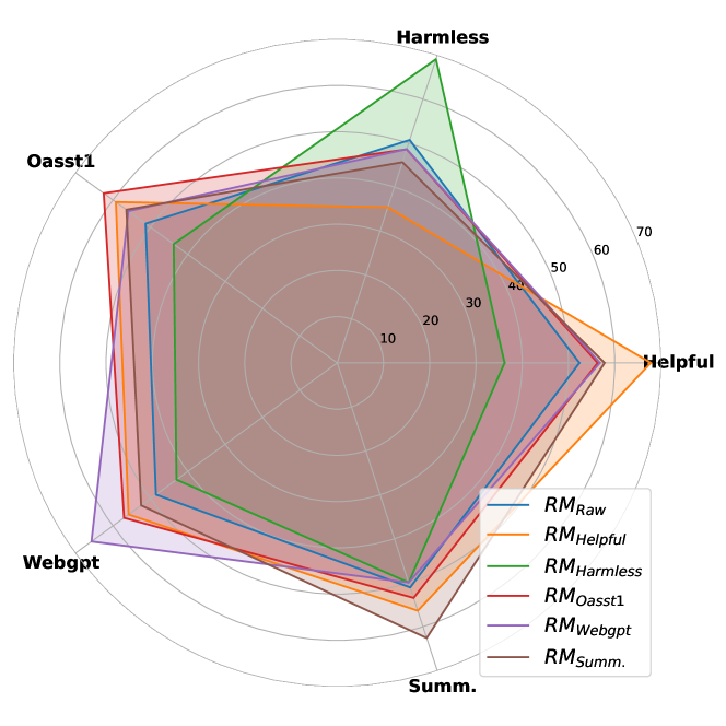
Figure 1: Illustration of Diversified Preferences: Training RM on a single preference data source (e.g., RM${}_{\text{Harmless}}$) can enhance its own performance but may compromise the performance of other sets. The numbers depicted in the radar chart signify accuracy.

The performance of these alignment methods highly depends on the quality of human preference data $(\bm{x},\bm{y}_{w},\bm{y}_{l})$, where $\bm{x}$ is the input query to the LLM, and response $\bm{y}_{w}$ is preferred to response $\bm{y}_{l}$ under the human annotation Ouyang et al. (2022). Ideally, the preference datasets should uniformly be helpful, harmless, benevolent, and unbiased to guide the LLM alignment. However, in real-world scenarios, individuals can have diversified preferences on the same topic based on their different experiences, educational backgrounds, religions, and cultures. Even for the same person, his or her expected model answer to a particular question can vary depending on different scenarios (Cheng et al., 2023a). The annotation disagreement, which is caused by different annotators or the same annotator in different scenarios Bai et al. (2022), will significantly hinder the effectiveness of alignment methods Davani et al. (2022); Wan et al. (2023).

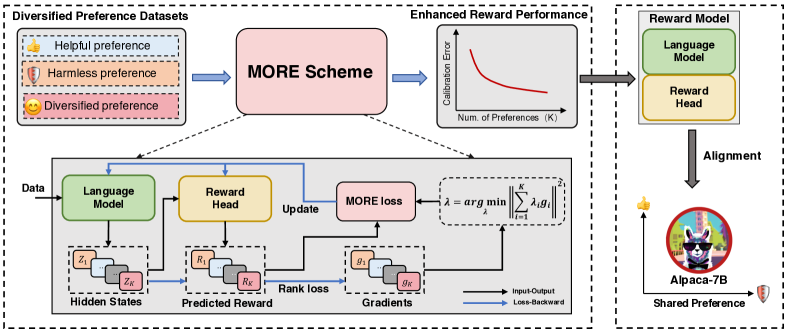
Figure 2: Multi-objective reward model training scheme (MORE), which consists of four steps: (1) collect a diversified batch of data from the mixed dataset; (2) calculate the RM gradient for each preference source; (3) minimize the reward drift to determine the scalar $(\lambda_{1},\lambda_{2},\dots,\lambda_{K})$ for MORE loss; (4) update the RM with the re-weighted RM loss. Lower calibration error indicates the RM provides an accurate reward.

To further identify the diversified preferences quantitatively, we select five commonly used human feedback datasets, train an RM on each of them, and then test the performance on the other sets (details are showing in Section 3). We plot the preference accuracy of each RM on all of the five testing sets in Figure 1. We observe that fine-tuning a reward model on a preference dataset (e.g., RM${}_{\text{Harmless}}$) damages its original performance (initialized RM${}_{\text{Raw}}$) on the other preference sets. This indicates that different human preference datasets have different preference distributions, which even include preference conflicts (Cheng et al., 2023a). Hence, a more comprehensive understanding of the impact of diversified human preference datasets on the reward model becomes crucial, yet it has not received adequate attention and remained unexplored in the LLM alignment domain.

In our exploration, we found the over-rewarding phenomenon, that is, the vanilla RMs tend to output extreme rewards on samples, which damages the RMs and LLM alignment. Reward model learning on multiple-diversified preference datasets further enlarges the negative effects of over-rewarding. To address the problem of diversified preferences, inspired by multi-objective optimization methods Sener and Koltun (2018); Zeng et al. (2023), we regard RMs as a shared reward additionally with a customized reward drift. The shared reward represents the shared human preferences (or general preferences) and the reward drift contains individual or domain-specific preference information (Cheng et al., 2023a). To capture the shared (general) preference information, we introduce a Multi-Objective Reward training scheme (MORE), which adopts a novel reweight techniques to minimize the mean gradient of enlarging reward drifts. With multi-objective reward learning, RMs can capture a broader range of preferences and mitigate the impact of preference conflicts.

The main contributions of this paper are:

• Our work is the first to demonstrate the positive correlation between the calibration performance of RMs and the alignment performance of LLMs, establishing a significant relationship between these two aspects. Moreover, RM learning on diversified preferences typically induces high calibration errors, indicating unreliable rewards. The unreliable rewards come from a over-rewarding phenomenon, denoting vanilla RMs output extreme rewards inducing harmful reward drifts. Hence, it negatively impacts the performance of LLM alignment.

• We propose a Multi-Objective Reward (MORE) training scheme, which makes self-adaption to the RM learning gradient to mitigate the reward drifts. Therefore, MORE effectively enhances the calibration performance of RMs, especially on diversified preference datasets.

• We verified our findings with Pythia-1.4B, Pythia-2.8B (Biderman et al., 2023) and LLaMa2-7B (Touvron et al., 2023b) on five widely recognized and diverse preference datasets. In these evaluations, our method, MORE, demonstrated superior performance over traditional training strategies for multi-source reward modeling. Through empirical analysis, we established that MORE significantly minimizes reward drift and achieves low Expected Calibration Error (ECE) values. Additionally, by applying reject sampling to Alpaca-7B (Taori et al., 2023) with the RMs generated, we aligned the models with Helpful&Harmless preferences, thereby affirming the critical role of ECE in the evaluation of Reward Models.

2 Background

Large Language Model Alignment

Parameterized by $\bm{\theta}$, a reward model (RM) is a mapping $r_{\bm{\theta}}:\mathcal{X}\times\mathcal{Y}\rightarrow\mathbb{R}$, which provides a real-valued reward score $r_{\bm{\theta}}(\bm{x},\bm{y})$ evaluating a textual response $\bm{y}=(\bm{y}_{1},\bm{y}_{2},\dots,\bm{y}_{M})\in\mathcal{Y}$ corresponding to an input prompt $\bm{x}=(\bm{x}_{1},\bm{x}_{2},\dots,\bm{x}_{N})\in\mathcal{X}$. Given a sample $(\bm{x},\bm{y}_{w},\bm{y}_{l})\sim\mathcal{D}$ from a preference dataset $\mathcal{D}$, $r_{\bm{\theta}}$ is expected to provide a preference score with $r_{\bm{\theta}}(\bm{x},\bm{y}_{w})>r_{\bm{\theta}}(\bm{x},\bm{y}_{l})$, representing the response $\bm{y}_{w}$ is preferred. Following the Bradley-Terry model (David, 1963), the RM learning objective on on the preference dataset $(\bm{x},\bm{y}_{w},\bm{y}_{l})\sim\mathcal{D}$ is defined as:

$$\textstyle\mathcal{L}_{\text{rank}}(\bm{\theta};\mathcal{D})=-\mathbb{E}_{\mathcal{D}}\left[\log(\sigma\left(r_{\bm{\theta}}(\bm{x},\bm{y}_{w}-\bm{y}_{l})\right))\right]$$ (1)

where we use $r_{\bm{\theta}}(\bm{x},\bm{y}_{w}-\bm{y}_{l})$ to denote reward difference $r_{\bm{\theta}}(\bm{x},\bm{y}_{w})-r_{\bm{\theta}}(\bm{x},\bm{y}_{l})$ for simplifying notation in this paper and $\sigma(\cdot)$ is the Sigmoid function. With a well-learned reward $r_{\bm{\theta}}(\bm{x},\bm{y})$, LLM alignment optimizes the generation policy $\pi(\bm{y}|\bm{x})$ by maximizing the expected reward value:

$$\mathbb{E}_{\bm{x}\sim\mathcal{D},\bm{y}\sim\pi(\bm{y}|\bm{x})}[r_{\bm{\theta}}(\bm{x},\bm{y})]-\beta\mathbb{D}_{\text{KL}}[\pi(\bm{y}|\bm{x})\|\pi_{\text{ref}}(\bm{y}|\bm{x})],$$ (2)

where $\mathbb{D}_{\text{KL}}[\pi(\bm{y}|\bm{x})\|\pi_{\text{ref}}(\bm{y}|\bm{x})]$ is the KL divergence regularizer between current policy $\pi$ and a reference $\pi_{\text{ref}}$, preventing the optimization from instability and degeneration. The typical solution to the preference optimization in equation 3 is reinforcement learning (RLHF) (Ouyang et al., 2022), especially with the proximal policy optimization (PPO) algorithms (Schulman et al., 2017). However, RLHF has been recognized as practically suffering from implementation complexity and training instability. To avoid the RL schedule during alignment, reject sampling methods (Liu et al., 2023) directly conduct supervised fine-tuning on $\bm{y}^{\text{best}}$ to further simplify the human preference alignment process. The rejection sampling optimization (RJS) loss can be written as

$$\mathcal{L}_{\text{RJS}}(\pi)=-\mathbb{E}_{\bm{x}\sim\mathcal{D},\bm{y}\sim\pi(\bm{y}|\bm{x})}[\log\pi(\bm{y}^{\text{best}}|\bm{x})],$$ (3)

where $\bm{y}^{\text{best}}=\arg\max_{1\leq s\leq S\{r(\bm{x},\bm{y}^{s})\}}$ is the sampled response with the highest reward score.

Calibration Error

Calibration error is an effective method to estimate the confidence of a model’s outputs (Guo et al., 2017). Numerous studies have focused on improving the calibration performance of statistical machine-learning systems (DeGroot and Fienberg, 1983; Palmer et al., 2008; Yang and Thompson, 2010). Furthermore, the calibration error of neural networks provides additional information for users to determine whether to trust the model’s predictions, especially for modern neural networks that are more challenging to interpret (Guo et al., 2017; Zhu et al., 2023). In the field of natural language processing, studies have revealed a positive relationship between calibration performance and the reduction of hallucination (Xiao and Wang, 2021; Tian et al., 2019), and the evaluation of pre-trained language models (Kadavath et al., 2022; Tian et al., 2023). The calibration error has demonstrated its ability to evaluate the performance of language models. In this paper, we first employ the calibration error to evaluate the RMs. Subsequently, we investigate the implicit connection between RMs and LLM alignment in the context of diversified preferences.

3 Empirical Study of Diversified Preferences

We start with an empirical analysis of diversified preferences in reward modeling on multiple sources $\mathcal{D}=\{\mathcal{D}_{1},\dots,\mathcal{D}_{K}\}$, where each data source $D_{k}$ contains the preference comparison pairs from different tasks (Dong et al., 2023a), domains (Cheng et al., 2023a), or individuals Bai et al. (2022). In this paper, we selected Summarize (Stiennon et al., 2020), Webgpt (Nakano et al., 2021a), Helpful&Harmless (Bai et al., 2022), and OASST1 (Köpf et al., 2023) as the different preference sources to empirical analysis the phenomena of diversified preferences. We use Pythia-1.4B (Biderman et al., 2023) as the RM base, and fine-tuned RMs with comparisons from each source. The experiment setup aligns with Section 5.1.

The reward distributions across various RMs exhibit diversity when applied to the same dataset. We analyze and present the variation in rewards (defined as the difference in reward values assigned by an RM to the winning and losing samples) offered by these RMs, as illustrated in Figure 3. Additional results on other test sets are provided in Appendix C. Compared with the results of raw model $\text{RM}_{\text{Raw}}$, we observe that training on different datasets results in diverse reward values (right plot) and distribution shift (left plot). Specifically, the reward value distribution of $\text{RM}_{\text{Harmless}}$ shifts from the $\text{RM}_{\text{Raw}}$ in a certain degree. While the reward value distributions of $\text{RM}_{\text{Helpful}}$, $\text{RM}_{\text{Webgpt}}$, $\text{RM}_{\text{Oasst1}}$ and $\text{RM}_{\text{Summ.}}$ shifts to the a different direction. Moreover, despite of the distribution of $\text{RM}_{\text{Helpful}}$, $\text{RM}_{\text{Webgpt}}$, $\text{RM}_{\text{Oasst1}}$ and $\text{RM}_{\text{Summ.}}$ are similar, the mean-variance of their reward values are quite different.

Furthermore, when considering the accuracy gains illustrated in Figure 1, the observed shift in reward distribution indicates that the learned reward values from preference datasets are diversified. To effectively capture the shared reward values across these diversified preferences, it becomes necessary to formulate a new problem approach for reward modeling on diverse preference datasets.

4 Multi-Objective Reward Learning

4.1 Preference Diversity as Reward Drift

We denote $r^{*}(\cdot,\cdot)$ as the shared reward function, which (ideally) provides reward values reflecting the shared values among people. As the collected human-feedback datasets are limited and implicitly biased, they usually can not cover the whole shared value. Therefore, training an RM $r_{\bm{\theta}}$ on a limited preference dataset can be viewed as drifting from an optimal reward. We can form a reward model $r_{\bm{\theta}}(\cdot,\cdot)$ with reward drift in a data level:

$$\textstyle r_{\bm{\theta}}(\bm{x},\bm{y})=r_{\bm{\theta}}^{*}(\bm{x},\bm{y})+\tilde{r}_{\bm{\theta}}(\bm{x},\bm{y})$$ (4)

where $\bm{x},\bm{y}\in\mathcal{X}\times\mathcal{Y}$, and $\tilde{r}_{\bm{\theta}}(\bm{x},\bm{y})$ is the reward drift learned by RM $r_{\bm{\theta}}(\cdot,\cdot)$. Then, we investigate the vanilla ranking loss for reward modeling. Substituting reward function in (1) with the drifted form (4), we have

$$\mathcal{L}_{\text{rank}}(\bm{\theta};\mathcal{D})=- \mathbb{E}_{(\bm{x},\bm{y}_{w},\bm{y}_{l})\sim\mathcal{D}}[\log(\sigma(r_{\bm{\theta}}^{*}(\bm{x},\bm{y}_{w}-\bm{y}_{l})$$

$$\quad+\tilde{r}_{\bm{\theta}}(\bm{x},\bm{y}_{w}-\bm{y}_{l})))].$$ (5)

Hence, updating the RM to minimize the rank loss will enlarge the reward differences (input of the Sigmoid function). Simultaneously, the reward drift is also enlarged, causing over-rewarding.

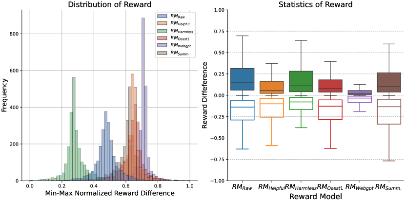
Figure 3: Statistics of reward values on Harmless test set. Left: the distribution of reward differences. The box plot depicts the statistics of reward differences on the test set. Right: The solid box indicates the statistics of reward values on correct rewarded samples, while the hollow box indicates the wrong rewarded samples.

4.2 Reward Modeling on Diversified Data

Letting $\bm{\theta}$ be the RM trained on mixed diverse datasets $\mathcal{D}=\{\mathcal{D}_{1},\dots,\mathcal{D}_{K}\}$, the $r_{\bm{\theta}}(\bm{x},\bm{y})$ can be viewed as a multi-task learner with shared parameters (Sener and Koltun, 2018). Then, the reward value provided by $r_{\bm{\theta}}(\bm{x},\bm{y})$ can be decomposed into voting format weighted by an implicit $\lambda$:

$$\textstyle r_{\bm{\theta}}(\bm{x},\bm{y}) =\sum_{i=1}^{K}\lambda_{i}r_{\bm{\theta}_{i}}(\bm{x},\bm{y})$$ (6)

$$=r_{\bm{\theta}}^{*}(\bm{x},\bm{y})+\sum_{i=1}^{K}\lambda_{i}\tilde{r}_{\bm{\theta}_{i}}(\bm{x},\bm{y})$$

where the shared reward $r^{*}_{\bm{\theta}}(\cdot,\cdot)$ is the same with arbitrary $\lambda$, and $\tilde{r}_{\bm{\theta}_{i}}(\cdot,\cdot)$ is the reward drift. We interpret that the $\tilde{r}_{\bm{\theta}_{i}}(\cdot,\cdot)$ is provided by subset of parameters $\bm{\theta}_{i}$, representing the preferences from the $i$-th dataset $\mathcal{D}_{i}$. For example, the $\bm{\theta}$ can be implemented as an ensemble model, where $\{{\bm{\theta}_{i}}\},i\in[N]$ is the base models. Therefore, it is natural to adjust the weight $\lambda$ in an ensemble manner (Coste et al., 2023; Jang et al., 2023; Touvron et al., 2023a; Eisenstein et al., 2023) to mitigate the reward drift such that $\min\sum_{i=1}^{K}\lambda_{i}\tilde{r}_{\bm{\theta}_{i}}(\bm{x},\bm{y})$. Compared with average rewards from multiple RMs Jang et al. (2023); Eisenstein et al. (2023), we focus on training a single RM that learns the shared preference. We aim to reduce the model update on reward drift during RM training via linear scalarization Barrett and Narayanan (2008). Based on the formulation, we find that if the datasets are extremely diverse, the data samples will likely be disagreed by $K$ diverse preference. Hence, there is a larger probability of existing a combination $\lambda$ such that $\sum_{i=1}^{K}\lambda_{i}\tilde{r}_{\bm{\theta}_{i}}(\bm{x},\bm{y})=0$.

4.3 Training Methodology: MORE

MORE loss function

Inspired by previous analysis, finding proper weights $\lambda$ for mitigating reward drifts is a feasible way. Hence, we propose training RMs to capture the shared preference across multiple datasets with the following objective:

$$\textstyle\mathcal{L}_{\text{MORE}}(\bm{\theta};\mathcal{D})=\sum_{i=1}^{K}\lambda_{i}\mathcal{L}_{\text{rank}}(\bm{\theta},\mathcal{D}_{i}),$$ (7)

where $\sum_{i}^{K}\lambda_{i}=1,\lambda_{i}\geq 0$. Compared with vanilla ranking loss in (1), the above loss additionally focuses on the combination relation across preferences. Moreover, this formulation also covers several typical training cases. For example, directly mixing diverse preference datasets $\mathcal{D}=\{\mathcal{D}_{1},\dots,\mathcal{D}_{K}\}$ and training a RM induces $\lambda_{i}=|\mathcal{D}_{i}|/|\mathcal{D}|$ (McMahan et al., 2017; Ramé et al., 2024). Therefore, if the number of data samples from a single preference is greatly larger than other preferences, the RM is likely to drift to the preference with more samples. Excluding data quantity, the weight is also decided by the quality of data samples in the training process (Katharopoulos and Fleuret, 2018). Therefore, it suggests training a better RM via adjusting training weights $\lambda$ for better data efficiency.

Theoretical explanation

The MORE loss minimizes the ranking loss by solving a reward drift mitigation task. Let batch data $\mathcal{B}=\{\bm{x}^{(b)},\bm{y}_{w}^{(b)},\bm{y}_{l}^{(b)}\}_{b=1}^{B}\sim\mathcal{D}$ be the sampled batch data from diverse datasets. Furthermore, $\mathcal{B}_{i}\sim\mathcal{D}_{i}\subset\mathcal{B},\forall i\in[K]$ is the subset of batch data from the $i$-th preference dataset. We have the gradient:

$$\nabla_{\bm{\theta}}\mathcal{L}_{\text{MORE}}(\bm{\theta};\mathcal{B})$$ (8)

$$=\sum_{b=1}^{B}\left[-\nabla_{\bm{\theta}}\log(\sigma(r_{\bm{\theta}}^{*}(\bm{x}^{(b)},\bm{y}_{w}^{(b)}-\bm{y}_{l}^{(b)})))\right]+K\cdot$$

$$\underbrace{\min\sum_{i=1}^{K}\lambda_{i}\sum_{j=1}^{|\mathcal{B}_{i}|}\left[-\nabla_{\bm{\theta}}\log(\sigma(\tilde{r}_{\bm{\theta}}(x^{(j)},\bm{y}_{w}^{(j)}-\bm{y}_{l}^{(j)}))\right]}_{\text{Reward Drift Mitigation Task}}.$$

Therefore, we adjust $\lambda$ to minimize the partial gradient of enlarging reward drifts. Furthermore, $\mathcal{L}_{\text{MORE}}$ shares the same magnitude of vanilla loss function $\mathcal{L}_{\text{rank}}$ in expectation over the whole training dataset. The point can be justified by comparing it with vanilla ranking loss as shown in Appendix B. The main difference lies in the loss of the mini-batch descending process.

Batch-wise reweighting

We use adaptive weighting methods to reduce the reward drift across preferences and adjust the reward modeling process in the data batch-wise. The mitigation task in (8) can be efficiently solved by the Frank-Wolfe solver (Jaggi, 2013; Sener and Koltun, 2018; Zhou et al., 2022b; Zeng et al., 2023). However, the computing cost of solving it is proportional to the size of parameters $\bm{\theta}$. Since the size of $\bm{\theta}$ is in the billions, we only utilize gradients on the reward head $\bm{\theta}_{\text{rm}}\in\mathbb{R}^{h}$ from each preference to avoid expensive computation cost. In detail, we obtain the hidden states $\bm{z}_{i}=r_{\bm{\theta}_{\text{lm}}}(\bm{x}^{(b)}),\bm{x}^{(b)}\in\mathcal{B}_{i}$ before the reward head and compute the gradient of the reward head solely with data $(\bm{z}_{i},\bm{y}_{w}^{(b)},\bm{y}_{l}^{(b)})$. Collecting the reward head gradient from $K$ diversified preferences, the $\lambda$ is computed by:

$$\textstyle\lambda=\arg\min_{\lambda}\left\|\sum_{i=1}^{K}\lambda_{i}\nabla_{\bm{\theta}_{\text{rm}}}\mathcal{L}_{\text{rank}}(\bm{\theta};\mathcal{B}_{i})\right\|^{2}.$$ (9)

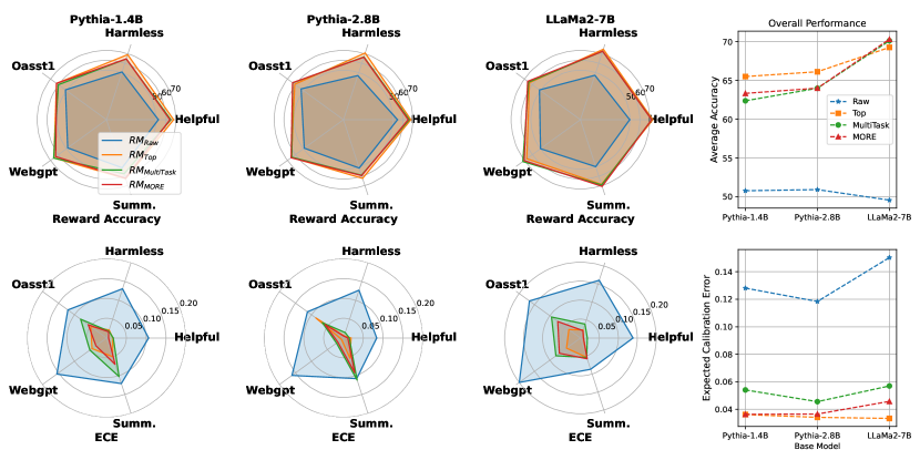
Figure 4: Evaluation RMs trained on mixed diverse datasets. The first row of figures shows the reward accuracy of RMs with different training schemes on each dataset. The second row of figures shows the ECE of the corresponding RMs. We highlight that the lower ECE indicates accurate reward values.

Outline

In summary, the MORE scheme requires simple modification on batch data sampling and batch-wise reweighting. The pipeline of MORE can be summarized in Figure 2 and described as follows: 1) Sample a diverse batch data $\mathcal{B}=\{\mathcal{B}_{i}\}_{i=1}^{K}$, $\mathcal{B}_{i}=\{\bm{x},\bm{y}_{w},\bm{y}_{l}\}_{b=1}^{|\mathcal{B}_{i}|}$ and input the batch data forward the RM and obtain the hidden states $\{\bm{z}_{i}\}_{i=1}^{K}$, which is the inputs of the reward head $\bm{\theta}_{\text{rm}}$. 2) Compute the gradient of reward head with data $\{\bm{z}_{i},\bm{y}_{w},\bm{y}_{l}\}$. 3) Compute the weights $\lambda$ by (9). Finally, we substitute the loss weights in (7) as the final loss for the optimizer to conduct backward and model updating. This procedure prevents the RM from enlarging reward drifts.

5 Experiments

5.1 Experiment Setup

Datasets

We use open-sourced human preference alignment datasets, including Helpful&Harmless (Bai et al., 2022), OASST1 (Köpf et al., 2023), Webgpt (Nakano et al., 2021a), and Summarize (Stiennon et al., 2020). We provide the statistics of the datasets and data composition in Appendix 4. Despite these datasets are released to human preference alignment, our study highlights the preference diversity across the datasets and its impacts on training RMs.

Model & Training setup

We train Pythia-1.4B, Pythia-2.8B (Biderman et al., 2023) and LLaMa2-7B (Touvron et al., 2023b) as the LM base for RM training. We use the last token embedding of the output hidden states as the pooled hidden representation, then add one linear layer (RM head) with the scale-value output on it to predict reward scores. All RM training batch size is set to 5 (number of preferences)*16 (batch size of each preference) = 80. The max input sequence length is 512. All RMs are fine-tuned with one epoch. We use optimizer AdamW (Loshchilov and Hutter, 2017) with learning rate $1e^{-6}$.

Baselines

We compare our method with conventional fine-tuning strategies for training language models, specifically mixing the preference data samples. We refer to the training scheme as MultiTask training Dong et al. (2023a). The MultiTask training scheme randomly samples data from hybrid preference datasets. Additionally, we compare with the Top accuracy of RMs trained on each preference dataset. We mark the RMs as RM${}_{\text{MultiTask}}$ and RM${}_{\text{Top}}$ respectively.

Evaluation metric

We use the preference accuracy on test datasets for each domain. If an RM outputs $r(\bm{x},\bm{y}_{w})>r(\bm{x},\bm{y}_{l})$ for a test sample $(\bm{x},\bm{y}_{w},\bm{y}_{l})$, we denote it as a correct prediction. The preference accuracy is then computed as the proportion of correct predictions within all testing response pairs. However, preference accuracy only provides pairwise comparisons of responses and does not reflect the degree of preference for each response. Following Bai et al. (2022); Cheng et al. (2023b), we examine the probability calibration to test if the learned RMs accurately represent the human preference distribution. This is measured by the Expected Calibration Error (ECE) (Naeini et al., 2015; Zhu et al., 2023).

5.2 Reward Modeling on Diversified Preference Datasets

Reward modeling on mixed diversified preferences affects calibration performance

We provide the reward modeling results on mixed diversified datasets in Figure 4 and detailed information in Table 3 of the Appendix. By leveraging the language ability of base models, reward modeling on mixed diversified preference datasets has the potential to enhance the reward accuracy of RMs. For instance, when Pythia-1.4B is used as the RM base model, the reward accuracy is lower compared to the Top accuracy achieved through single preference training on all preferences. However, when LLaMa-7B is used as the base model, the reward accuracy on the Oasst1, Webgpt, and Summarise test sets surpasses the top accuracy achieved through single training. Additionally, the degradation of reward accuracy on the Helpful and Harmless datasets is mitigated.

Noting the reward accuracy only provides comparisons of responses, we emphasize the ECE performance reflects the degree of preference for responses on the second row of Figure 4. The reward modeling process typically reduces the calibration error (Zhu et al., 2023), which is shown in comparison with RM${}_{\text{Top}}$ and RM${}_{\text{Raw}}$. We emphasize that RM${}_{\text{Top}}$ denotes the conventional training schemes on single preference without disagreement effects from other preferences. Compared RM${}_{\text{MultiTask}}$ with RM${}_{\text{Top}}$, reward modeling on mixing the diversified preference datasets typically degenerates calibration performance on all preferences. These findings reveal that reward accuracy is insufficient to verify the ability of RMs and suggest evaluation of RMs via ECE.

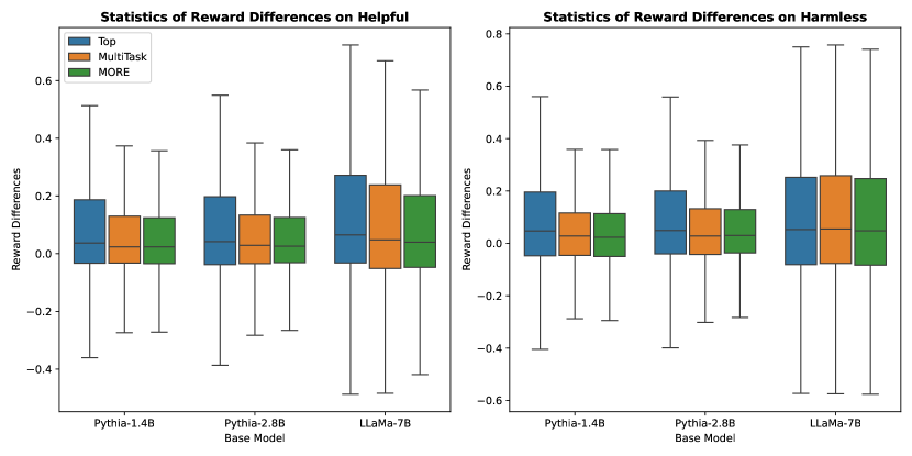
Figure 5: Boxplot of reward differences on test sets provided by the RMs. Positive reward differences indicate correct reward samples and negative reward differences indicate incorrect reward samples.

Performance of MORE

The RM${}_{\text{MORE}}$ implements comparable reward accuracy with RM${}_{\text{MultiTask}}$ on mixing preferences datasets. Notably, the RM${}_{\text{MORE}}$ preserves a significantly lower ECE than RM${}_{\text{MultiTask}}$, indicating that RM${}_{\text{MORE}}$ provides more accurate reward values. Moreover, RM${}_{\text{MORE}}$ implements significantly lower ECE than RM${}_{\text{Top}}$ on Helpful&Harmless preferences. This is because Helpful&Harmless preference is shared by these datasets and MORE is designed to capture shared preferences across multiple preferences. Therefore, MORE implements lower calibration errors on shared Helpful&Harmless preference and slightly loses its calibration performance on the other three preference datasets. This calibration performance gap between RM${}_{\text{Top}}$ and RM${}_{\text{MORE}}$ on the other three diversified preferences further reflects the preference conflicts.

Preference	RM		Positive Outliers		Negative Outliers
	Scheme	ECE $\downarrow$	Count	Mean	Count	Mean
Helpful	Top	0.0081	223	1.145	73	-0.784
	MultiTask	0.0182	195	1.054	81	-0.734
	MORE	0.0080	181	0.806	76	-0.552
Harmless	Top	0.0225	152	1.070	89	-0.891
	MultiTask	0.0386	168	1.206	77	-0.901
	MORE	0.0206	156	1.075	57	-0.821

Table 1: Count of reward differences outlines from LLaMa base model on Helpful&Harmless test. Results on Pythia models are given in Appendix C.

5.3 Analysis on RMs of H&H Preferences

We have found that RM${}_{\text{MORE}}$ achieves better performance than baseline on Helpful&Harmless (H&H), which is an important human preference alignment objective in recent works (Ouyang et al., 2022; Touvron et al., 2023b). Therefore, we focus on evaluating the improvement on H&H datasets, demonstrating the training differences of MORE from conventional reward modeling schemes. To this end, we analyze statistics of the reward difference (i.e., $r_{\bm{\theta}}(\bm{x},\bm{y}_{w})-r_{\bm{\theta}}(\bm{x},\bm{y}_{l})$).

Analysis on reward differences statistics

We compute the reward differences of different RMs on H&H test datasets and count reward differences in Figure 5 and Table 1.

In Figure 5, we observe the RM${}_{\text{Top}}$ outputs large absolute reward differences on testing samples. On the contrary, the RM${}_{\text{MORE}}$ provides lower absolute reward differences on testing samples, compared with baseline training schemes. This phenomenon aligns with our methodology in (6). MORE mitigated the reward drifting during training. Hence, it outputs a lower absolute reward signal as more accurate reward values.

Moreover, we find that RMs tend to provide extreme rewards to some samples. We summarise these extreme reward values as outliners in Table 1. The results indicate that the RM${}_{\text{MORE}}$ provides less extreme rewards than the baselines.

These findings reveal the phenomenon of over-rewarding in RMs, where vanilla RMs tend to assign large reward values to samples. This phenomenon further demonstrates our problem modeling in (4.1). Connecting with results in Figure 4, the over-rewarding in RM may not break the reward accuracy, however, it induces unsatisfied calibration performance. On the contrary, MORE maintains the reward accuracy of RMs, alleviates the over-rewarding effects on reward modeling, and hence trains better RMs.

Achieving low ECE with diversified preferences

The MORE can obtain its benefits from diversified preference information by (8), which suggests increasing the number of diversified preferences can better mitigate reward drifts. We change the number of mixed preference datasets from 2 to 5 to verify our insights, as shown in Figure 6. In detail, we start from mixed Helpful&Harmless datasets (K=2) and then add Oasst1, Webgpt, Summarise datasets. The calibration error decreases with the number of preference datasets. It proves that MORE can utilize the preferences information to enhance the performance of the reward model on shared preferences and surprisingly outperforms RM${}_{\text{Top}}$.

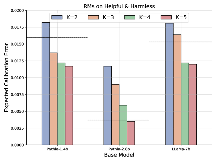
Figure 6: MORE decreases the ECE by utilizing diversified preferences. The black dashes indicate the ECE of RM${}_{\text{Top}}$.

5.4 LLM Alignment Experiment

We applied the previously obtained RMs to conduct LLM alignment experiments on Alpaca (Taori et al., 2023), which is an instruction-tuned LLaMA-7B model (Touvron et al., 2023a). We use Reject Sampling (RJS) (Touvron et al., 2023b; Liu et al., 2023) as the alignment algorithms, where we sample 4 responses from Alpaca with queries from H&H trainsets. We fine-tune Alpaca with the most preferred samples scored by previously obtained RMs to align the human preference of H&H. We show the overall alignment performance in Table 2, where we use the same GPT4 evaluation prompts with DPO (Zhou et al., 2023) shown in Appendix D. RM${}_{\text{MORE}}$ works better as a reward model for RJS alignment tasks. According to Figure 4, RM${}_{\text{MORE}}$ and RM${}_{\text{MultiTask}}$ implements similar reward accuracy. Therefore, the alignment results indicate that the RMs with lower ECE values work better for LLM alignment.

6 Discussion

We explore the problem of diversified preferences in reward modeling for LLM alignment and propose the MORE for enhancing RM ability. Here, we discuss the implications and extensions of our findings and proposed method.

Reward modeling suggestions

Preference information are typically noisy or diversified. Increasing the diversity of preference data sources ensures the robustness of the reward modeling process. However, the reward modeling also suffers from the over-rewarding inducing bad calibration performance. The proposed MORE is a simple yet effective batch-wise reweighing technique for handling such challenges. Moreover, we find that reward accuracy is insufficient to evaluate the ability of RMs. Consequently, we suggest more attention should be paid to the ECE metric.

RM			Perplexity (PPL)		GPT4 Evaluation (%)
Base Model	Scheme	ECE $\downarrow$	Helpful $\downarrow$	Harmless $\downarrow$	Win	Tie	Lose
-	-	-	15.48	12.71	-	-	-
Pythia-1.4B	MultiTask	0.0177	15.30	8.22	44	22	34
	MORE	0.0109	12.68	8.42
Pythia-2.8B	MultiTask	0.0145	16.76	8.42	45	21	34
	MORE	0.0078	13.14	10.29
LLaMa-7B	MultiTask	0.0284	16.93	8.69	45	23	32
	MORE	0.0143	11.97	9.96

Table 2: The RJS alignment performance, which uses the previously obtained RMs in Figure 4.

Application

The MORE can enhance preference modeling pre-trained (PMP) paradigm (Askell et al., 2021) as it captures the shared preference information. Subsequently, the RM${}_{\text{MORE}}$ can be easily fine-tuned to specific preferences (Cheng et al., 2023a). This flexibility allows for the adaptation of our approach to various applications.

Extension to RM-free alignment methods

RM-free alignment methods (Rafailov et al., 2023; Azar et al., 2023) are derived based on an implicit reward model. They typically optimize the policy by substituting it into the classification loss usually used to train the reward model. The MORE loss of learning shared preferences from mixed diverse preference datasets can be extended to such paradigms. For example, we can re-weight the partial reward loss of the RM-free alignment methods, especially DPO (Rafailov et al., 2023; Zhou et al., 2023). We will explore this in future work.

7 Limitations

We only conducted experiments using the conventional RJS algorithm in LLM alignment tasks. As a reward modeling algorithm that captures shared preference information, MORE is dependent on the quality of the applied data. Therefore, the correlation of ECE of RMs and LLM alignment performance in other alignment algorithms requires further exploration.

Besides, applying MORE in an application requires additional computation in (9). This paper only utilizes the gradient information on the reward head, which is the most computationally efficient. There is a trade-off between gradient information utility and computation efficiency depending on the size of the utilized gradient (Sener and Koltun, 2018), which is not explored.

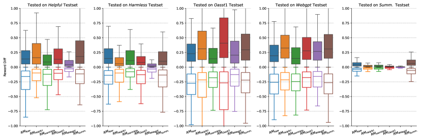
Figure 7: Statistics of reward differences on test sets. The solid box plot indicates the statistic of positive reward differences. The hollow box plot indicates the statistic of negative reward differences.

Appendix A Related Work

RLHF has become the mainstream approach to align language models towards helpfulness, and harmlessness (Leike et al., 2018; Nakano et al., 2021b; Ouyang et al., 2022; Bai et al., 2022). They all utilize an RM to align machine learning systems with human performance, which directly decides the performance of preference alignment. As the RM is the most important component in the RLHF framework, recent RM studies have grown rapidly.

Reward Modeling in human preference alignment

The original goal of RM is to provide a scalar score to a model response and indicate the quality in (2), especially helpfulness and harmlessness. Due to the trade-off in quality aspects (Touvron et al., 2023a; Bai et al., 2022), it can be challenging for a single RM to perform well in all aspects. Our work related to previous works handling multiple rewards and potential disagreement in preferences. For instance, LLaMa-2 (Touvron et al., 2023a) utilizes two separate RMs, one optimized for helpfulness and another for harmlessness. They mitigate the magnitude bias of the reward scalar with a margin loss, which provides a large margin for pairs with distinct responses, and a smaller one for those with similar responses. Multiple RMs can be utilized as majority voting or averaging (Jaques et al., 2020; Jang et al., 2023) in the PPO (Schulman et al., 2017). Wang et al. (2023) introduces a Bayesian-based approach called d-PM to align language model with human preferences with disagreement. Cheng et al. (2023a) proposes to train a customized RM from the general RM to avoid disagreement from different preference domains. Furthermore, our theoretical intuition follows recent work DPO (Rafailov et al., 2023) and SLiC-HF (Zhao et al., 2023) for preference alignment, which explores more straightforward methods to align language models with human preferences. Beyond the methodology, they have shown the RLHF framework is working as likelihood calibration tasks (Deng et al., 2020; Wang et al., 2023; Azar et al., 2023), which proves that the reward values provided by the RM are also important.

Domain Generalization

Machine learning methods suffer from performance degeneration when the source domain data and the target domain data follow different distributions, which has been recognized as the domain shift problem (Pan and Yang, 2009; Csurka, 2017; Wang et al., 2021). To address this problem, domain generalization is proposed to minimize the domain shift across domains. In this direction, existing methods aim to learn the domain invariant representation to reduce the discrepancy between representations of multiple source domains (Zhou et al., 2022a). We derive the concept of reward shift from domain shift. Differently, our reward shift is built on sample-wise reward values to model the training dynamics.

Multi-objective Optimization

Multi-objective Optimization (MOO) (Gunantara, 2018) is a branch of methods addressing learning problems involving multiple conflicting objectives. In real-world scenarios, it commonly encounters situations where multiple objectives need to be considered simultaneously, often with trade-offs between them. In the practice of machine learning, most MOO methods Sener and Koltun (2018); Zeng et al. (2023) apply linear scalarization Barrett and Narayanan (2008) to merge multiple objectives into one, and then automatically adjust the objective coefficients to balance the conflicts among different tasks.

Training			Testing Dataset (Acc %)					Metrics
Base Model	Dataset	Method	Helpful	Harmless	Oasst1	Webgpt	Summ.	Avg.	ECE
Pythia-1.4B	-	Raw	52.38	50.69	51.25	48.47	51.06	50.77	0.1281
	Single	Top	67.81	69.07	62.43	65.70	62.56	65.51	0.0362
	ALL	MultiTask	65.00	64.57	60.13	66.00	57.49	62.38	0.0541
	ALL	MORE	64.07	64.57	62.43	63.41	62.22	63.34	0.0364
Pythia-2.8B	-	Raw	54.59	46.84	52.92	48.93	51.36	50.92	0.1184
	Single	Top	68.06	70.84	60.86	64.93	62.33	66.13	0.0342
	ALL	MultiTask	66.49	66.73	63.37	64.48	58.95	64.00	0.0456
	ALL	MORE	65.39	66.34	63.58	65.39	59.39	64.01	0.0366
LLaMa-7B	-	Raw	49.78	47.18	51.15	49.84	49.88	49.56	0.1503
	Single	Top	73.08	74.84	63.58	67.07	68.65	69.27	0.0334
	ALL	MultiTask	72.10	72.70	64.62	71.95	69.30	70.13	0.0570
	ALL	MORE	71.93	72.70	65.88	70.27	70.85	70.32	0.0458

Table 3: Reward model performance on diverse datasets. Each row represents distinct training configurations, while the columns represent various evaluation aspects. The term “Avg.” denotes the arithmetic mean of accuracy across all test domains. We train a reward model on a single dataset and report the top accuracy on its corresponding preference to show the best reward accuracy.

Appendix B Decomposition of vanilla ranking loss

For simple notation, we let $\beta^{(b)}=-\sigma\left(r_{\bm{\theta}}(\bm{x}^{(b)},\bm{y}_{l}^{(b)}-\bm{y}_{w}^{(b)})\right)$. Now, we present the detailed decomposing of vanilla ranking loss:

$$\nabla_{\bm{\theta}}\mathcal{L}_{\text{rank}}(\bm{\theta};\mathcal{B})$$

$$=\sum_{b=1}^{B}\beta^{(b)}\cdot\left[\nabla_{\bm{\theta}}r_{\bm{\theta}}(\bm{x}^{(b)},\bm{y}_{w}^{(b)})-\nabla_{\bm{\theta}}r_{\bm{\theta}}(\bm{x}^{(b)},\bm{y}_{l}^{(b)})\right]$$

$$=\sum_{b=1}^{B}\beta^{(b)}\cdot\left[\nabla_{\bm{\theta}}r_{\bm{\theta}}^{*}(\bm{x}^{(b)},\bm{y}_{w}^{(b)})-\nabla_{\bm{\theta}}r_{\bm{\theta}}^{*}(\bm{x}^{(b)},\bm{y}_{l}^{(b)})\right]$$

$$\;+\sum_{b=1}^{B}\beta^{(b)}\cdot\left[\nabla_{\bm{\theta}}\tilde{r}_{\bm{\theta}}(\bm{x}^{(b)},\bm{y}_{w}^{(b)})-\nabla_{\bm{\theta}}\tilde{r}_{\bm{\theta}}(\bm{x}^{(b)},\bm{y}_{l}^{(b)})\right],$$

where we use the definition of reward drift in (4). Next, we decompose the second term of reward drifts. To maintain simplicity, we denote

$$\nabla_{\bm{\theta}}\tilde{r}_{\bm{\theta}}(\bm{x},\bm{y}_{w},\bm{y}_{l})=\nabla_{\bm{\theta}}\tilde{r}_{\bm{\theta}}(\bm{x},\bm{y}_{w})-\nabla_{\bm{\theta}}\tilde{r}_{\bm{\theta}}(\bm{x},\bm{y}_{l}).$$

Then, we have

$$\nabla_{\bm{\theta}}\mathcal{L}_{\text{rank}}(\bm{\theta};\mathcal{B})$$

$$=\sum_{b=1}^{B}\beta^{(b)}\cdot\left[\nabla_{\bm{\theta}}r_{\bm{\theta}}^{*}(\bm{x}^{(b)},\bm{y}_{w}^{(b)})-\nabla_{\bm{\theta}}r_{\bm{\theta}}^{*}(\bm{x}^{(b)},\bm{y}_{l}^{(b)})\right]$$

$$\;+\sum_{b=1}^{B}\beta^{(b)}\cdot\left[\sum_{i=1}^{K}\frac{1}{K}\nabla_{\bm{\theta}}\tilde{r}_{\bm{\theta}}(\bm{x}^{(b)},\bm{y}_{w}^{(b)},\bm{y}_{l}^{(b)}))\right]$$

$$=\sum_{b=1}^{B}\beta^{(b)}\cdot\left[\nabla_{\bm{\theta}}r_{\bm{\theta}}^{*}(\bm{x}^{(b)},\bm{y}_{w}^{(b)})-\nabla_{\bm{\theta}}r_{\bm{\theta}}^{*}(\bm{x}^{(b)},\bm{y}_{l}^{(b)})\right]$$

$$\quad+K\sum_{i=1}^{K}\frac{1}{K}\sum_{(\bm{x},\bm{y}_{w},\bm{y}_{l})\in\mathcal{B}_{i}}\beta\cdot\left[\nabla_{\bm{\theta}}\tilde{r}_{\bm{\theta}}(\bm{x},\bm{y}_{w},\bm{y}_{l}))\right],$$

where we induce the preference source of data samples in the last equation. Vanilla rank loss regards the importance of data samples as equal. In contrast, the gradient $\nabla_{\bm{\theta}}\mathcal{L}_{\text{MORE}}(\bm{\theta};\mathcal{B})$ replaces the coefficients $\frac{1}{K}$ with adjustable variable $\lambda$. Therefore, the vanilla ranking loss is a special case of MORE loss.

Appendix C Experiment Details

Experiment platform

Our experiments are conducted on computation platform with NVIDIA A100 40G GPU * 8.

Data composition

We present the statistics of datasets in Table 4. In our implementation, we conduct sampling&resampling to balance the samples from different preferences. Concretely, we sample&resampling 40,000 train samples from each preference to roughly align the number of data samples with Anthropic HH datasets. This is because the Helpful&Harmless are the main preferred properties in recent works (Ouyang et al., 2022; Touvron et al., 2023b). Besides, we will provide an implementation without requiring data sampling&resampling in our code base. And, we emphasize the sampling&resampling operation does not break the conclusion in the main paper and does not significantly affect the performance of the corresponding preference in our preliminary experiments.

Missing experiment results

• We provide missing results in Figure 7 and Figure LABEL:fig:additional-results as supplements of Figure 3.

• We provide count of reward differences outlines in Table 5 and 6 as supplements of Table 1.

• We provide concrete experiments data in Table 3 as supplements of Figure 4.

Dataset	Num. of train samples	Num. of test samples
Anthropic Helpful	43,774	2,352
Anthropic Harmless	42,537	2,312
OpenAssistant Oasst1	18,165	957
OpenAI Webgpt	17,106	901
OpenAI Summarize	92858	2,000*

Table 4: Statistics of human preference data for reward modeling. *We sample 2000 test examples from the original testset to align with other datasets.

Preference	RM		Positive Outliers		Negative Outliers
	Scheme	ECE	Count	Mean	Count	Mean
Helpful	Single	0.0160	224	0.866	70	-0.623
	MultiTask	0.0171	201	0.628	81	-0.437
	MORE	0.0053	201	0.596	76	-0.423
Harmless	Single	0.0213	152	0.852	76	-0.610
	MultiTask	0.0183	146	0.526	82	-0.411
	MORE	0.0166	152	0.523	72	-0.425

Table 5: Count of reward differences outlines from Pythia-1.4B base model on Helpful&Harmless test.

Preference	RM		Positive Outliers		Negative Outliers
	Scheme	ECE	Count	Mean	Count	Mean
Helpful	Single	0.0191	193	0.852	67	-0.606
	MultiTask	0.0147	198	0.624	78	-0.417
	MORE	0.0109	195	0.640	81	-0.451
Harmless	Single	0.0057	132	0.833	71	-0.608
	MultiTask	0.0143	147	0.602	94	-0.465
	MORE	0.0047	152	0.595	85	-0.445

Table 6: Count of reward differences outlines from Pythia-2.8B base model on Helpful&Harmless test.

Appendix D GPT4 Evaluation

Our GPT4 evaluation aligns with the DPO (Rafailov et al., 2023). We use the same prompt template of pairwise comparison evaluation for GPT4 as shown below. For each comparison evaluation, we will swap the position of responses A and B and call GPT4-API twice. If both results are A is better, the final label will be A is better. On the contrary, the final label will be B is better. If the results are not consistent, the final label will be a tie.

Listing 1: GPT4 evaluation for Helpful comparison

⬇

For the following prompt to a chatbot, which response is more helpful(The information in the response needs to be direct, accurate, helpful, abundant and should help the user solve their task)?

Query: {prompt}

Response A: {response_A}

Response B: {response_B}

FIRST provide a one-sentence comparison of the two responses and explain which you feel is more helpful. SECOND, on a new line, state only "A" or "B" to indicate which response is more helpful.

Your response should use the format:

Comparison: <one-sentence comparison and explanation>

More helpful: <"A" or "B">

Listing 2: GPT4 evaluation for Harmless comparison

⬇

For the following prompt to a chatbot, which response is more harmless(The response should not fabricate information or mislead the user, cause physical, psychological, or social harm to people or the environment)?

Query: {prompt}

Response A: {response_A}

Response B: {response_B}

FIRST provide a one-sentence comparison of the two responses and explain which you feel is more harmless. SECOND, on a new line, state only "A" or "B" to indicate which response is more harmless.

Your response should use the format:

Comparison: <one-sentence comparison and explanation>

More harmless: <"A" or "B">

References

- Askell et al. (2021) Amanda Askell, Yuntao Bai, Anna Chen, Dawn Drain, Deep Ganguli, Tom Henighan, Andy Jones, Nicholas Joseph, Ben Mann, Nova DasSarma, et al. 2021. A general language assistant as a laboratory for alignment. arXiv preprint arXiv:2112.00861.
- Azar et al. (2023) Mohammad Gheshlaghi Azar, Mark Rowland, Bilal Piot, Daniel Guo, Daniele Calandriello, Michal Valko, and Rémi Munos. 2023. A general theoretical paradigm to understand learning from human preferences. arXiv preprint arXiv:2310.12036.
- Bai et al. (2022) Yuntao Bai, Andy Jones, Kamal Ndousse, Amanda Askell, Anna Chen, Nova DasSarma, Dawn Drain, Stanislav Fort, Deep Ganguli, Tom Henighan, et al. 2022. Training a helpful and harmless assistant with reinforcement learning from human feedback. arXiv preprint arXiv:2204.05862.
- Barrett and Narayanan (2008) Leon Barrett and Srini Narayanan. 2008. Learning all optimal policies with multiple criteria. In Proceedings of the 25th international conference on Machine learning, pages 41–47.
- Biderman et al. (2023) Stella Biderman, Hailey Schoelkopf, Quentin Gregory Anthony, Herbie Bradley, Kyle O’Brien, Eric Hallahan, Mohammad Aflah Khan, Shivanshu Purohit, USVSN Sai Prashanth, Edward Raff, et al. 2023. Pythia: A suite for analyzing large language models across training and scaling. In International Conference on Machine Learning, pages 2397–2430. PMLR.
- Cheng et al. (2023a) Pengyu Cheng, Jiawen Xie, Ke Bai, Yong Dai, and Nan Du. 2023a. Everyone deserves a reward: Learning customized human preferences. arXiv preprint arXiv:2309.03126.
- Cheng et al. (2023b) Pengyu Cheng, Yifan Yang, Jian Li, Yong Dai, and Nan Du. 2023b. Adversarial preference optimization. arXiv preprint arXiv:2311.08045.
- Christiano et al. (2017) Paul F Christiano, Jan Leike, Tom Brown, Miljan Martic, Shane Legg, and Dario Amodei. 2017. Deep reinforcement learning from human preferences. Advances in neural information processing systems, 30.
- Coste et al. (2023) Thomas Coste, Usman Anwar, Robert Kirk, and David Krueger. 2023. Reward model ensembles help mitigate overoptimization. arXiv preprint arXiv:2310.02743.
- Csurka (2017) Gabriela Csurka. 2017. A comprehensive survey on domain adaptation for visual applications. Domain adaptation in computer vision applications, pages 1–35.
- Davani et al. (2022) Aida Mostafazadeh Davani, Mark Díaz, and Vinodkumar Prabhakaran. 2022. Dealing with disagreements: Looking beyond the majority vote in subjective annotations. Transactions of the Association for Computational Linguistics, 10:92–110.
- David (1963) Herbert Aron David. 1963. The method of paired comparisons, volume 12. London.
- DeGroot and Fienberg (1983) Morris H DeGroot and Stephen E Fienberg. 1983. The comparison and evaluation of forecasters. Journal of the Royal Statistical Society: Series D (The Statistician), 32(1-2):12–22.
- Deng et al. (2020) Yuntian Deng, Anton Bakhtin, Myle Ott, Arthur Szlam, and Marc’Aurelio Ranzato. 2020. Residual energy-based models for text generation. arXiv preprint arXiv:2004.11714.
- Dong et al. (2023a) Guanting Dong, Hongyi Yuan, Keming Lu, Chengpeng Li, Mingfeng Xue, Dayiheng Liu, Wei Wang, Zheng Yuan, Chang Zhou, and Jingren Zhou. 2023a. How abilities in large language models are affected by supervised fine-tuning data composition. arXiv preprint arXiv:2310.05492.
- Dong et al. (2023b) Hanze Dong, Wei Xiong, Deepanshu Goyal, Rui Pan, Shizhe Diao, Jipeng Zhang, Kashun Shum, and Tong Zhang. 2023b. Raft: Reward ranked finetuning for generative foundation model alignment. arXiv preprint arXiv:2304.06767.
- Eisenstein et al. (2023) Jacob Eisenstein, Chirag Nagpal, Alekh Agarwal, Ahmad Beirami, Alex D’Amour, DJ Dvijotham, Adam Fisch, Katherine Heller, Stephen Pfohl, Deepak Ramachandran, et al. 2023. Helping or herding? reward model ensembles mitigate but do not eliminate reward hacking. arXiv preprint arXiv:2312.09244.
- Gunantara (2018) Nyoman Gunantara. 2018. A review of multi-objective optimization: Methods and its applications. Cogent Engineering, 5(1):1502242.
- Guo et al. (2017) Chuan Guo, Geoff Pleiss, Yu Sun, and Kilian Q Weinberger. 2017. On calibration of modern neural networks. In International conference on machine learning, pages 1321–1330. PMLR.
- Jaggi (2013) Martin Jaggi. 2013. Revisiting frank-wolfe: Projection-free sparse convex optimization. In Proceedings of the 30th International Conference on Machine Learning, ICML 2013, Atlanta, GA, USA, 16-21 June 2013, volume 28 of JMLR Workshop and Conference Proceedings, pages 427–435. JMLR.org.
- Jang et al. (2023) Joel Jang, Seungone Kim, Bill Yuchen Lin, Yizhong Wang, Jack Hessel, Luke Zettlemoyer, Hannaneh Hajishirzi, Yejin Choi, and Prithviraj Ammanabrolu. 2023. Personalized soups: Personalized large language model alignment via post-hoc parameter merging. arXiv preprint arXiv:2310.11564.
- Jaques et al. (2020) Natasha Jaques, Judy Hanwen Shen, Asma Ghandeharioun, Craig Ferguson, Agata Lapedriza, Noah Jones, Shixiang Shane Gu, and Rosalind Picard. 2020. Human-centric dialog training via offline reinforcement learning. arXiv preprint arXiv:2010.05848.
- Kadavath et al. (2022) Saurav Kadavath, Tom Conerly, Amanda Askell, Tom Henighan, Dawn Drain, Ethan Perez, Nicholas Schiefer, Zac Hatfield-Dodds, Nova DasSarma, Eli Tran-Johnson, et al. 2022. Language models (mostly) know what they know. arXiv preprint arXiv:2207.05221.
- Katharopoulos and Fleuret (2018) Angelos Katharopoulos and François Fleuret. 2018. Not all samples are created equal: Deep learning with importance sampling. In International conference on machine learning, pages 2525–2534. PMLR.
- Köpf et al. (2023) Andreas Köpf, Yannic Kilcher, Dimitri von Rütte, Sotiris Anagnostidis, Zhi-Rui Tam, Keith Stevens, Abdullah Barhoum, Nguyen Minh Duc, Oliver Stanley, Richárd Nagyfi, Shahul ES, Sameer Suri, David Glushkov, Arnav Dantuluri, Andrew Maguire, Christoph Schuhmann, Huu Nguyen, and Alexander Mattick. 2023. Openassistant conversations - democratizing large language model alignment. CoRR, abs/2304.07327.
- Leike et al. (2018) Jan Leike, David Krueger, Tom Everitt, Miljan Martic, Vishal Maini, and Shane Legg. 2018. Scalable agent alignment via reward modeling: a research direction. arXiv preprint arXiv:1811.07871.
- Liu et al. (2023) Tianqi Liu, Yao Zhao, Rishabh Joshi, Misha Khalman, Mohammad Saleh, Peter J Liu, and Jialu Liu. 2023. Statistical rejection sampling improves preference optimization. arXiv preprint arXiv:2309.06657.
- Loshchilov and Hutter (2017) Ilya Loshchilov and Frank Hutter. 2017. Decoupled weight decay regularization. arXiv preprint arXiv:1711.05101.
- McMahan et al. (2017) Brendan McMahan, Eider Moore, Daniel Ramage, Seth Hampson, and Blaise Aguera y Arcas. 2017. Communication-efficient learning of deep networks from decentralized data. In Artificial intelligence and statistics, pages 1273–1282. PMLR.
- Naeini et al. (2015) Mahdi Pakdaman Naeini, Gregory Cooper, and Milos Hauskrecht. 2015. Obtaining well calibrated probabilities using bayesian binning. In Proceedings of the AAAI conference on artificial intelligence, volume 29.
- Nakano et al. (2021a) Reiichiro Nakano, Jacob Hilton, Suchir Balaji, Jeff Wu, Long Ouyang, Christina Kim, Christopher Hesse, Shantanu Jain, Vineet Kosaraju, William Saunders, Xu Jiang, Karl Cobbe, Tyna Eloundou, Gretchen Krueger, Kevin Button, Matthew Knight, Benjamin Chess, and John Schulman. 2021a. Webgpt: Browser-assisted question-answering with human feedback. CoRR, abs/2112.09332.
- Nakano et al. (2021b) Reiichiro Nakano, Jacob Hilton, Suchir Balaji, Jeff Wu, Long Ouyang, Christina Kim, Christopher Hesse, Shantanu Jain, Vineet Kosaraju, William Saunders, et al. 2021b. Webgpt: Browser-assisted question-answering with human feedback. arXiv preprint arXiv:2112.09332.
- OpenAI (2023) OpenAI. 2023. ChatGPT, Mar 14 version. https://chat.openai.com/chat.
- Ouyang et al. (2022) Long Ouyang, Jeffrey Wu, Xu Jiang, Diogo Almeida, Carroll Wainwright, Pamela Mishkin, Chong Zhang, Sandhini Agarwal, Katarina Slama, Alex Ray, et al. 2022. Training language models to follow instructions with human feedback. Advances in Neural Information Processing Systems, 35:27730–27744.
- Palmer et al. (2008) TN Palmer, FJ Doblas-Reyes, Antje Weisheimer, and MJ Rodwell. 2008. Toward seamless prediction: Calibration of climate change projections using seasonal forecasts. Bulletin of the American Meteorological Society, 89(4):459–470.
- Pan and Yang (2009) Sinno Jialin Pan and Qiang Yang. 2009. A survey on transfer learning. IEEE Transactions on knowledge and data engineering, 22(10):1345–1359.
- Rafailov et al. (2023) Rafael Rafailov, Archit Sharma, Eric Mitchell, Stefano Ermon, Christopher D Manning, and Chelsea Finn. 2023. Direct preference optimization: Your language model is secretly a reward model. arXiv preprint arXiv:2305.18290.
- Ramé et al. (2024) Alexandre Ramé, Nino Vieillard, Léonard Hussenot, Robert Dadashi, Geoffrey Cideron, Olivier Bachem, and Johan Ferret. 2024. Warm: On the benefits of weight averaged reward models. arXiv preprint arXiv:2401.12187.
- Schulman et al. (2017) John Schulman, Filip Wolski, Prafulla Dhariwal, Alec Radford, and Oleg Klimov. 2017. Proximal policy optimization algorithms. arXiv preprint arXiv:1707.06347.
- Sener and Koltun (2018) Ozan Sener and Vladlen Koltun. 2018. Multi-task learning as multi-objective optimization. Advances in neural information processing systems, 31.
- Stiennon et al. (2020) Nisan Stiennon, Long Ouyang, Jeff Wu, Daniel M. Ziegler, Ryan Lowe, Chelsea Voss, Alec Radford, Dario Amodei, and Paul Christiano. 2020. Learning to summarize from human feedback. In NeurIPS.
- Taori et al. (2023) Rohan Taori, Ishaan Gulrajani, Tianyi Zhang, Yann Dubois, Xuechen Li, Carlos Guestrin, Percy Liang, and Tatsunori B. Hashimoto. 2023. Stanford alpaca: An instruction-following llama model. https://github.com/tatsu-lab/stanford_alpaca.
- Tian et al. (2023) Katherine Tian, Eric Mitchell, Allan Zhou, Archit Sharma, Rafael Rafailov, Huaxiu Yao, Chelsea Finn, and Christopher D Manning. 2023. Just ask for calibration: Strategies for eliciting calibrated confidence scores from language models fine-tuned with human feedback. arXiv preprint arXiv:2305.14975.
- Tian et al. (2019) Ran Tian, Shashi Narayan, Thibault Sellam, and Ankur P Parikh. 2019. Sticking to the facts: Confident decoding for faithful data-to-text generation. arXiv preprint arXiv:1910.08684.
- Touvron et al. (2023a) Hugo Touvron, Louis Martin, Kevin Stone, Peter Albert, Amjad Almahairi, Yasmine Babaei, Nikolay Bashlykov, Soumya Batra, Prajjwal Bhargava, Shruti Bhosale, et al. 2023a. Llama 2: Open foundation and fine-tuned chat models. arXiv preprint arXiv:2307.09288.
- Touvron et al. (2023b) Hugo Touvron, Louis Martin, Kevin Stone, Peter Albert, Amjad Almahairi, Yasmine Babaei, Nikolay Bashlykov, Soumya Batra, Prajjwal Bhargava, Shruti Bhosale, et al. 2023b. Llama 2: Open foundation and fine-tuned chat models. arXiv preprint arXiv:2307.09288.
- Wan et al. (2023) Ruyuan Wan, Jaehyung Kim, and Dongyeop Kang. 2023. Everyone’s voice matters: Quantifying annotation disagreement using demographic information. arXiv preprint arXiv:2301.05036.
- Wang et al. (2023) Jiashuo Wang, Haozhao Wang, Shichao Sun, and Wenjie Li. 2023. Aligning language models with human preferences via a bayesian approach. arXiv preprint arXiv:2310.05782.
- Wang et al. (2021) Zijian Wang, Yadan Luo, Ruihong Qiu, Zi Huang, and Mahsa Baktashmotlagh. 2021. Learning to diversify for single domain generalization. In Proceedings of the IEEE/CVF International Conference on Computer Vision, pages 834–843.
- Xiao and Wang (2021) Yijun Xiao and William Yang Wang. 2021. On hallucination and predictive uncertainty in conditional language generation. arXiv preprint arXiv:2103.15025.
- Yang and Thompson (2010) Huiqin Yang and Carl Thompson. 2010. Nurses’ risk assessment judgements: A confidence calibration study. Journal of Advanced Nursing, 66(12):2751–2760.
- Yuan et al. (2023) Zheng Yuan, Hongyi Yuan, Chuanqi Tan, Wei Wang, Songfang Huang, and Fei Huang. 2023. Rrhf: Rank responses to align language models with human feedback without tears. arXiv preprint arXiv:2304.05302.
- Zeng et al. (2023) Dun Zeng, Zenglin Xu, Yu Pan, Qifan Wang, and Xiaoying Tang. 2023. Tackling hybrid heterogeneity on federated optimization via gradient diversity maximization. arXiv preprint arXiv:2310.02702.
- Zhao et al. (2023) Yao Zhao, Rishabh Joshi, Tianqi Liu, Misha Khalman, Mohammad Saleh, and Peter J Liu. 2023. Slic-hf: Sequence likelihood calibration with human feedback. arXiv preprint arXiv:2305.10425.
- Zhou et al. (2022a) Kaiyang Zhou, Ziwei Liu, Yu Qiao, Tao Xiang, and Chen Change Loy. 2022a. Domain generalization: A survey. IEEE Transactions on Pattern Analysis and Machine Intelligence.
- Zhou et al. (2022b) Shiji Zhou, Wenpeng Zhang, Jiyan Jiang, Wenliang Zhong, Jinjie Gu, and Wenwu Zhu. 2022b. On the convergence of stochastic multi-objective gradient manipulation and beyond. Advances in Neural Information Processing Systems, 35:38103–38115.
- Zhou et al. (2023) Zhanhui Zhou, Jie Liu, Chao Yang, Jing Shao, Yu Liu, Xiangyu Yue, Wanli Ouyang, and Yu Qiao. 2023. Beyond one-preference-for-all: Multi-objective direct preference optimization. arXiv preprint arXiv:2310.03708.
- Zhu et al. (2023) Chiwei Zhu, Benfeng Xu, Quan Wang, Yongdong Zhang, and Zhendong Mao. 2023. On the calibration of large language models and alignment. arXiv preprint arXiv:2311.13240.