Parametric estimation of quantile versions of Zenga and D inequality curves: methodology and application to Weibull distribution

Abstract.

Inequality (concentration) curves such as Lorenz, Bonferroni, Zenga curves, as well as a new inequality curve — the $D$ curve, are broadly used to analyse inequalities in wealth and income distribution in certain populations. Quantile versions of these inequality curves are more robust to outliers. We discuss several parametric estimators of quantile versions of the Zenga and $D$ curves. A minimum distance (MD) estimator is proposed for these two curves and the indices related to them. The consistency and asymptotic normality of the MD estimator is proved. The MD estimator can also be used to estimate the inequality measures corresponding to the quantile versions of the inequality curves. The estimation methods considered are illustrated in the case of the Weibull model, which is often applied to the precipitation data or times to the occurrence of a certain event.

1. Introduction

Inequality curves, for example the Lorenz curve [26], are broadly used to analyse inequalities of wealth and income distribution in certain populations (see e.g. [2]). Dozens of other applications in various fields of science appeared in recent years, which leads to the idea of proposing some alternatives for the most popular inequality curve, i.e. the Lorenz curve, and for associated with it an inequality measure, which is the Gini index. Lorenz curve is not defined for distributions with infinite expected value and is sensitive to outliers. Some alternatives, like the Bonferroni curve [5], the Zenga-07 curve [40] and $D$ curve [10], are defined by their relationship with the Lorenz curve, and for this reason they share these drawbacks.

Prendergast and Staudte proposed three quantile versions of the Lorenz curve that could also be applied to the distributions with infinite mean value [29]. Some methods of estimating these curves were described by Siedlaczek [34]. In [30] Prendergast and Staudte also proposed the $R$ curve and elaborated on its properties, estimation, and possible applications. They also suggested an alternative curve, which together with the $R$ curve after a minor transform gives quantile counterparts of the Zenga and $D$ curves, respectively, denoted here as the $qZ$ and $qD$ curves. The problem of nonparametric estimation of $qZ$ and $qD$ was covered by Jokiel-Rokita and Piątek in [21].

In this paper we focus on the problem of parametric estimation of two quantile concentration curves, namely $qZ$, which is an alternative to the Zenga curve [40] and $qD$, an alternative to the $D$ curve [10]. Let $X$ be a nonnegative random variable with cumulative distribution function (cdf) $F_{\theta}(t)=P_{\theta}(X\leq t),$ where ${\theta}\in\Theta$ is an unknown parameter. Denote by

$$Q_{\theta}(p)=F_{\theta}^{-1}(p)=\inf\{t\in\mathbb{R}:F_{\theta}(t)\geq p\}$$

the quantile function (qf). The $qZ$ and $qD$ concentration curves are defined as follows:

$$qZ(p;Q_{\theta})=1-\frac{Q_{\theta}(p/2)}{Q_{\theta}((1+p)/2)},\qquad p\in(0,1)$$

and

$$qD(p;Q_{\theta})=1-\frac{Q_{\theta}(p/2)}{Q_{\theta}(1-p/2)},\qquad p\in(0,1).$$

In addition, these curves are defined at the extreme points $p=0$ and $p=1$ as follows:

$$qZ(0;Q_{\theta})=1=qZ(1;Q_{\theta}),\quad qD(0;Q_{\theta})=1\quad\text{and}\quad qD(1;Q_{\theta})=0.$$

The perfect equality curve for $qZ$ and for $qD$ is equal to 0. An illustration of the example curves $qZ$ and $qD$ for the Weibull distribution with several values of the shape parameter is depicted in Figure 1. The concentration indices $qZI(Q_{\theta})$ and $qDI(Q_{\theta})$ are defined as the area under curves $qZ$ and $qD$, respectively, that is

$$qZI(Q_{\theta})=\int_{0}^{1}qZ(p;Q_{\theta})\,dp,$$

$$qDI(Q_{\theta})=\int_{0}^{1}qD(p;Q_{\theta})\,dp.$$

Some applications of these indices to the salary data were presented in [21] and [6].

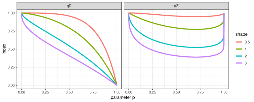
Figure 1. Comparison of the $qD$ (left plot) and $qZ$ (right plot) for Weibull distribution with different values of shape parameter

The article is organised as follows. Section 2 provides the definition of the proposed minimum distance estimator of the $qZ$ and $qD$ curves. In Section 3 the properties of the minimum distance estimators are proved. Section 4 introduces the Weibull distribution, which can be used as an example of a model for which $qZ$ and $qD$ can be estimated with MD estimators. Section 5 provides a comparison of several estimators of the $qZ$ and $qD$ curves in case of data from the Weibull distribution. In Section 6 an analysis of a real data set with the concentration curves is given. The last section contains a brief summary of this paper.

2. Minimum distance estimator

One of the possible methods that can be used to estimate the $qZ$ and $qD$ curves is the minimum distance (MD) method. It was introduced by Wolfowitz (see for example [38]) and has been widely used since then. More information on minimum distance estimation can be found in Basu et al. [3] and references therein. Millar described [28] the minimum distance-type estimators of the parameter $\theta\in\Theta$ of a distribution given with $F_{\theta}$ as follows. Denote by $\mathcal{H}$ the Hilbert space of the real bounded functions on $\mathbb{R}$. Let $F_{\theta},{F}_{n}\in\mathcal{H}$ and let $|\cdot|_{\mathcal{H}}$ be the norm of $\mathcal{H}$. A minimum distance estimator of $\theta$ based on cdf is $\hat{\theta}$ such that

$$\hat{\theta}=\operatorname{arg\,inf}_{\theta\in\Theta}|\xi_{n}(\theta)|_{\mathcal{H}},$$

where $\xi_{n}(\theta)$ is a stochastic process with time parameter $\theta\in\Theta$ and values in $\mathcal{H}$. The process $\xi_{n}$ can be defined in various ways as a difference between a function of a true parameter and its empirical counterpart. For example, $\xi_{n}$ could be $|F_{\theta}-{F}_{n}|_{\mathcal{H}}$. Since the goal here is to estimate the function $qZ(p;Q_{\theta})$, one can define an MD estimator of $\theta$ based on the $qZ$ curve. This estimator $\hat{\theta}$ is found by minimising the distance between $qZ_{\theta}=qZ(p;Q_{\theta})$ and the empirical curve denoted by

(1) $$qZ_{n}=qZ(p;Q_{n}),$$

so it yields a curve $qZ_{\hat{\theta}}=qZ(p;Q_{\hat{\theta}})$ that should best match the empirical curve. $Q_{n}$ stands here for empirical qf, given by

$${Q}_{n}(p;{\bf X}):=\inf\{t:F_{n}(t;{\bf X})\geq p\},$$

where $F_{n}$ is the empirical cdf. We can define a process

$$\xi_{n}^{E}(\theta)=qZ_{n}-qZ_{\theta}.$$

The formal definition of the MD estimator of the parameter $\theta$ obtained this way is as follows:

(2) $$\hat{\theta}^{E}_{n}=\operatorname{arg\,inf}_{\theta\in\Theta}|\xi_{n}^{E}(\theta)|_{B}.$$

The most common choice of the norm of $\mathcal{H}$ in the problem of minimum distance estimation is $L_{2}$ norm, which was used, for example, to define MD estimators of the ODC curve [17], the ROC curve (see for example [9], [22], [15] or [23]) or parameters of the $\alpha$-stable distribution (see [16] or [13]).

Similarly, another MD estimator can be obtained basing on difference between $qZ_{\theta}$ and another nonparametric estimator of $qZ$. For example, a continuous counterpart of $qZ_{n}$ can be considered. Jokiel-Rokita and Piątek [21] suggested to use to estimate both $qZI$ and $qDI$ a nonparametric plug-in estimator based on the Hyndman and Fan estimator (HF) [18] of qf ($Q_{n}^{HF}$) when the finiteness of the expected value of the random variable is assumed. Weibull and Gumbel estimator (WG) [18] of qf was recommended in the opposite case. These estimators are defined as a linear interpolation between plotting positions $(p_{k},X_{(k)})$, where

$$p_{k}^{HF}=\frac{k-1/3}{n+1/3}\qquad\text{and}\qquad p_{k}^{WG}=\frac{k}{n+1},$$

respectively for HF and WG estimators and $X_{(k)}$ is the $k$-th order statistic. In the intervals $[0,p_{1}]$ and $[p_{n},1]$ such estimators have values $X_{(1)}$ and $X_{(n)}$ respectively. In consecutive sections only HF estimator is considered to maintain the clarity of the work, but WG estimator and some similar continuous counterparts of empirical qf may be used. Considering $qZ_{n}^{HF}$, defined by plugging-in the HF estimator of qf into the formula for $qZ$, we get

(3) $$\hat{\theta}^{HF}=\operatorname{arg\,inf}_{\theta\in\Theta}|\xi_{n}^{HF}(\theta)|_{B},$$

where

$$\xi_{n}^{HF}(\theta)=qZ_{n}^{HF}-qZ_{\theta}.$$

Remark 2.1.

Analogous MD estimators can also be constructed for the $qD$ curve based on its empirical estimator $qD_{n}$ or the continuous estimator $qD_{n}^{HF}$.

3. Properties of the estimators

In this section, the proofs of existence and asymptotic properties of MD estimators of $qZ$ (for a given $p$) and $qZI$ (and $qD$ and $qDI$) are given. To provide the proofs we recall stochastic processes $\xi_{n}^{E}(\theta)$ and $\xi_{n}^{HF}(\theta)$ defined in Section 2. We denote by $T$ the continuous linear operator from $\Theta$ to $\mathcal{H}$, for which

(4) $$\xi_{n}^{E}(\theta)=\xi_{n}^{E}(\theta_{0})+T(\theta-\theta_{0})+o_{P}(\theta-\theta_{0}),$$

$$\xi_{n}^{HF}(\theta)=\xi_{n}^{HF}(\theta_{0})+T(\theta-\theta_{0})+o_{P}(\theta-\theta_{0}),$$

where $\theta_{0}$ is the true value of the parameter $\theta$. Using Taylor’s formula we can show that

(5) $$T(\theta)=\theta\frac{d}{d\theta_{0}}\left(qZ_{\theta_{0}}\right).$$

Let

(6) $$\eta(\theta_{0})=\frac{d}{d\theta_{0}}\left(qZ_{\theta_{0}}\right)$$

and $\mathcal{B_{\eta}}$ be the linear space spanned by $\eta(\theta_{0})$. Let $\pi$ be the orthogonal projection from $\mathcal{H}$ to $\mathcal{B_{\eta}}$. Now we introduce the following lemmas.

Lemma 3.1.

If $F$ is differentiable at $F^{-1}(t)$, for a given $t$, with positive derivative $Q^{{}^{\prime}}(t)=f(F^{-1}(t))$, then the process $\sqrt{n}\,\xi_{n}^{E}(\theta)$ converges in distribution to

$$G^{E}(t;\theta)=\left[1-qZ(t)\right]\left[\frac{Q^{{}^{\prime}}\left(\frac{t}{2}\right)}{Q\left(\frac{t}{2}\right)}B\left(\frac{t}{2}\right)-\frac{Q^{{}^{\prime}}\left(\frac{1+t}{2}\right)}{Q\left(\frac{1+t}{2}\right)}B\left(\frac{1+t}{2}\right)\right],$$

where $B$ is the standard Brownian bridge.

This lemma was proved as Theorem (5.7) in [21].

Lemma 3.2.

Under the assumptions of Lemma 3.1, we have

$$\sup_{t\in[0,1]}|Q_{n}(t)-Q_{n}^{HF}(t)|=O_{P}\left(\frac{1}{n}\right).$$

Proof.

Let us notice that

$$\sup_{t\in[0,1]}|Q_{n}(t)-Q_{n}^{HF}(t)|\leq\sup_{1\leq k,m<n}|p_{k}^{E}-p_{k}^{HF}||X_{(m+1)}-X_{(m)}|.$$

The left factor is $O\left(\frac{1}{n}\right)$, since

$$\sup_{1\leq k\leq n}|p_{k}^{E}-p_{k}^{HF}|=\sup_{1\leq k\leq n}\frac{\frac{1}{3}(k+n)}{n(n+\frac{1}{3})}=O_{P}\left(\frac{1}{n}\right).$$

The latter is $O_{P}\left(1\right)$, because for any $p\in[m/n,(m+1)/n]$ we have

$$\sup_{1\leq m<n} |X_{(m+1)}-X{(m)}|$$

$$=\sup_{1\leq m<n,p\in[m/n,(m+1)/n]}|X_{(m+1)}-Q(p+1/n)+Q(p+1/n)-Q(p)+Q(p)-X{(m)}|$$

$$\leq\sup_{1\leq m<n,p\in[m/n,(m+1)/n]}|X_{(m+1)}-Q(p+1/n)|$$

$$+\sup_{p\in[0,1]}|Q(p+1/n)-Q(p)|+\sup_{1\leq m<n,p\in[m/n,(m+1)/n]}|Q(p)-X{(m)}|.$$

The first and third component of the above sum are $O_{P}(1)$, since the empirical quantile converges in probability to the true quantile. The middle one is $O_{P}\left(\frac{1}{n}\right)$, from the definition of the derivative of $Q$ in the point $p$. Thus, $\sup_{t\in[0,1]}|Q_{n}(t)-Q_{n}^{HF}(t)|$ is $O_{P}\left(\frac{1}{n}\right)$. ∎

Lemma 3.3.

Under the assumptions of Lemma 3.1, we have

$$\sup_{t\in[0,1]}|qZ_{n}(t)-qZ_{n}^{HF}(t)|=O_{P}\left(\frac{1}{n}\right).$$

Proof.

We have

$$\sup_{t\in[0,1]} |qZ_{n}(t)-qZ_{n}^{HF}(t)|$$

$$=\sup_{t\in[0,1]}\left|\frac{Q_{n}\left(\frac{t}{2}\right)}{Q_{n}\left(\frac{t+1}{2}\right)}-\frac{Q_{n}^{HF}\left(\frac{t}{2}\right)}{Q_{n}\left(\frac{t+1}{2}\right)}+\frac{Q_{n}^{HF}\left(\frac{t}{2}\right)}{Q_{n}\left(\frac{t+1}{2}\right)}-\frac{Q_{n}^{HF}\left(\frac{t}{2}\right)}{Q_{n}^{HF}\left(\frac{t+1}{2}\right)}\right|$$

$$\leq\sup_{t\in[0,1]}\left|\frac{1}{Q_{n}\left(\frac{t+1}{2}\right)}\right|\left|Q_{n}\left(\frac{t}{2}\right)-Q_{n}^{HF}\left(\frac{t}{2}\right)\right|$$

$$\qquad+\left|\frac{Q_{n}^{HF}\left(\frac{t}{2}\right)}{Q_{n}\left(\frac{t+1}{2}\right)Q_{n}^{HF}\left(\frac{t+1}{2}\right)}\right|\sup_{t\in[0,1]}\left|Q_{n}\left(\frac{t+1}{2}\right)-Q_{n}^{HF}\left(\frac{t+1}{2}\right)\right|$$

$$\leq\frac{2}{Q_{n}(\frac{1}{2})}\sup_{t\in[0,1]}|Q_{n}(t)-Q_{n}^{HF}(t)|.$$

Following Corrolary 21.5 in [36] we have

$$Q_{n}(p)=Q(p)-\frac{1}{n}\sum_{i=1}^{n}\frac{\mathbbm{1}\{X_{i}\leq Q(p)\}-p}{f(Q(p))}+O_{P}(n^{-1/2}),$$

thus $Q_{n}(p)=Q(p)+O_{P}(n^{-1/2})$, so the factor $2/Q_{n}(\frac{1}{2})$ is $O_{P}(1)$. The second factor $\sup_{t\in[0,1]}|Q_{n}(t)-Q_{n}^{HF}(t)|$ is $O_{P}(\frac{1}{n})$, following Lemma 3.2. Thus $\sup_{t\in[0,1]}|qZ_{n}(t)-qZ_{n}^{HF}(t)|$ is $O_{P}(\frac{1}{n})$. ∎

The asymptotic properties of the MD estimators $\xi_{n}^{E}(\theta)$ and $\xi_{n}^{HF}(\theta)$ are given in following theorem.

Theorem 3.4.

Let us assume the identifiability, convergence, differentiability and boundedness of $\xi_{n}^{E}(\theta)$. We denote by $\hat{\theta}^{E}$ the MD estimator (2). Then with probability approaching to 1 with $n\to\infty$, the estimator $\hat{\theta}^{E}$ exists and is unique. Moreover for $\hat{\theta}^{E}$ we have

$$\xi_{n}^{E}(\hat{\theta}^{E}_{n})=(1-\pi)\circ\xi_{n}^{E}(\theta_{0})+o_{P}(n^{-1/2}),$$

$$\hat{\theta}^{E}_{n}-\theta_{0}=-T^{-1}\circ\pi\circ\xi_{n}^{E}(\theta_{0})+o_{P}(n^{-1/2}),$$

$$\sqrt{n}\left(\xi_{n}^{E}(\hat{\theta}^{E}_{n})-\xi_{n}^{E}(\theta_{0})\right)\xrightarrow{d}\pi\circ G^{E}(t;\theta_{0})\,\,\text{in}\,\mathcal{H},$$

(7) $$\sqrt{n}\left(\hat{\theta}^{E}_{n}-\theta_{0}\right)\xrightarrow{d}-T^{-1}\circ\pi\circ G^{E}(t;\theta_{0})\,\,\text{in}\,\mathbb{R}^{d}.$$

Proof.

The proof is based on Theorem (3.6) from Millar’s work [28]. In order to use this theorem, we need to check the four assumptions about the process $\xi_{n}^{E}(\theta)$. The first one, identifiability, is fulfilled since $\xi_{n}^{E}(\theta)-\xi_{n}^{E}(\theta_{0})=qZ_{\theta}(t)-qZ_{\theta_{0}}(t)$ which is not random and does not depend on $n$. The convergence was shown in Lemma 3.1. The differentiability is given by the existence of $T$ defined as in (5) which satisfies (4). Finally, $\xi_{n}^{E}(\theta)$ is obviously bounded. All the assumptions are satisfied, thus the theorem is proved. ∎

Remark 3.5.

Following Lemma 3.3 the difference between $qZ_{n}$ and $qZ_{n}^{HF}$ is of $O_{P}\left(\frac{1}{n}\right)$, thus all these properties also hold for $\hat{\theta}^{HF}$ defined in (3).

Corollary 3.6.

The MD estimator $\hat{\theta}_{n}$ from the previous theorem is asymptotically normal with mean $0$ and variance given in the proof.

Proof.

As we can see in equation (7), the asymptotic distribution of $\hat{\theta}$ can also be obtained. Following Millar (see equation (2.20) in [28]) we have the variance of the MD estimator $\hat{\theta}_{n}^{E}$ given by

$$\sigma_{E}^{2}=C^{-1}AC,$$

where $C$ and $A$ are matrices with entries

$$C_{ij}=\int_{0}^{1}\eta_{i}(t)\eta_{j}(t)\,dt,\qquad A_{ij}=\int_{0}^{1}\int_{0}^{1}\eta_{i}(s)\eta_{j}(t)R(s,t)\,ds\,dt,$$

which reduces in one-dimensional case to

$$\sigma_{E}^{2}=A=\int_{0}^{1}\int_{0}^{1}\eta(s)\eta(t)R(s,t)\,ds\,dt.$$

The function $\eta$ is defined as in (6) and $R(s,t)$ denotes here the covariance function of $G^{E}(t;\theta)$, which is equal to

$$R(s,t) =a(t)a(s)\left(\frac{1}{2}\min\{t,s\}-\frac{ts}{4}\right)-b(t)a(s)\left(\frac{s}{2}-\frac{(1+t)s}{4}\right)$$

$$+b(t)b(s)\left(\frac{1}{2}(1+\min\{t,s\})-\frac{(1+t)(1+s)}{4}\right)-a(t)b(s)\left(\frac{t}{2}-\frac{(1+s)t}{4}\right),$$

where

$$a(t)=\left[1-qZ(t)\right]\frac{Q^{{}^{\prime}}\left(\frac{t}{2}\right)}{Q\left(\frac{t}{2}\right)}\qquad\text{and}\qquad b(t)=\left[1-qZ(t)\right]\frac{Q^{{}^{\prime}}\left(\frac{1+t}{2}\right)}{Q\left(\frac{1+t}{2}\right)}.$$

∎

Denote the plug-in estimators of $qZ$ curve $\widehat{qZ}^{E}(p;{\bf X})=qZ(p;Q_{\hat{\theta}^{E}})$ and $\widehat{qZ}^{HF}(p;{\bf X})=qZ(p;Q_{\hat{\theta}^{HF}})$ and plug-in estimators of $qZI$.

Corollary 3.7.

The estimators $\widehat{qZ}^{E}(p;{\bf X})$ and $\widehat{qZ}^{HF}(p;{\bf X})$ are consistent estimators of $qZ(p;Q)$ for every $p\in[0,1]$.

Proof.

This is a consequence of applying the delta method (see for example Chapter 3 in [36]), which can be done, since $qZ(p;Q_{\hat{\theta}})$ is a continuous function of $\theta$ for each $p\in[0,1]$. ∎

Corollary 3.8.

The estimators $\widehat{qZI}^{E}({\bf X})$ and $\widehat{qZI}^{HF}({\bf X})$ are consistent estimators of $qZI(Q)$.

Proof.

From the definition of $\widehat{qZI}^{E}({\bf X})$ and $qZI(Q),$ we have

$$\widehat{qZI}^{E}({\bf X})-qZI(Q)=\int_{0}^{1}\left[\widehat{qZ}^{E}(p;{\bf X})-qZ(p;Q)\right]\,dp.$$

We have though

$$\int_{0}^{1}\left[\widehat{qZ}^{E}(p;{\bf X})-qZ(p;Q)\right]\,dp\leq\sup_{p\in(0,1)}|\widehat{qZ}^{E}(p;{\bf X})-qZ(p;Q)|.$$

The right-hand side of the inequality above converges to 0 when $n$ tends to infinity, since the estimator $\widehat{qZ}^{E}(p;{\bf X})$ is a consistent estimator of $qZ$ for each $p\in[0,1]$. Thus $\widehat{qZI}^{E}({\bf X})$ converges in probability to $qZI(Q)$. The proof for $\widehat{qZ}^{HF}$ follows the same pattern. ∎

Remark 3.9.

All the properties shown in this section for $qZ$ also hold for $qD$ and can be proved analogously.

Remark 3.10.

MD estimators of parameter $\theta$ based on empirical $qZ$ can also be used to construct a plug-in estimator of $qD$ and vice versa.

4. Weibull distribution

The two-parameter Weibull distribution $\mathcal{W}(\beta,\sigma)$ is defined by the probability density function

$$f(x)=\frac{\beta}{\sigma}\left(\frac{x}{\sigma}\right)^{\beta-1}\exp\Big{[}-\left(\frac{x}{\sigma}\right)^{\beta}\Big{]},\quad x\geq 0,\beta>0,\sigma>0,$$

where $\sigma$ is a scale parameter and $\beta$ is a shape parameter [37].

4.1. Concentration curves and measures for the Weibull distribution

This distribution is utilised for example to fit precipitation data [19], travel times [1] or time intervals of the first passage process of foreign exchange rates [31, 7]. The Gini index sometimes appears as a measure used to analyse inequalities in such data [12, 31, 25]. Lorenz curve is also applied in reliability problems [8], where the Weibull distribution often appears.

The qf of the Weibull distribution is given by

$$Q(p)=\sigma\left[-\log(1-p)\right]^{1/\beta}.$$

Thus, the curves $qZ$ and $qD$ for the Weibull distribution are

$$qZ(p;\beta)=1-\left[\frac{\log(1-p/2)}{\log((1-p)/2)}\right]^{1/\beta}$$

and

$$qD(p;\beta)=1-\left[\frac{\log(1-p/2)}{\log(p/2)}\right]^{1/\beta},$$

respectively, hence they are scale invariant and depend only on the shape parameter $\beta$.

Figure 2 depicts the relation between the shape parameter of the Weibull distribution and the values of three indices, namely the already mentioned $qZI$ and $qDI$, as well as the Gini index ($GI$). It can be deduced from this plot that $GI$ is more volatile then other two indices when the shape parameter $\beta$ is small (smaller than 2), however $qZI$ and $qDI$ might tend to be more susceptible (than $GI$) to the changes of $\beta$ when it is greater than 2.

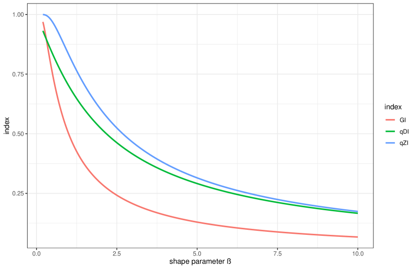
Figure 2. Comparison of the $GI$, $qZI$ and $qDI$ for different values of shape parameter of Weibull distribution

4.2. Plug-in estimators based on estimators of the shape parameter

A plug-in estimators of $qZ$ and $qZI$, having $\mathbf{X}=(X_{1},\ldots,X_{n})$ which is a random sample from Weibull distribution, are defined by

$$\widehat{qZ}(p;{\bf X})=1-\left[\frac{\log(1-p/2)}{\log(1/2-p/2)}\right]^{1/\hat{\beta}}$$

and

$$\widehat{qZI}({\bf X})=\int_{0}^{1}\widehat{qZ}(p;{\bf X})\,dp,$$

where $\hat{\beta}$ is an estimator of the shape parameter $\beta$ of the Weibull distribution.

Although the MD estimators of the parameter $\beta$ and aforementioned concentration curves and measures have desired properties, some standard estimators of $\beta$ might lead to plug-in estimators of curves and measures having lower MSE and MISE. The popular methods of estimation of parameter $\beta$ were compared in many works in terms of their bias and MSE, but there are not much papers about the problem of estimation of curves depending on the parameters of the Weibull distribution, which can be estimated with a plug-in estimator. Thus in the simulation study in Section 5 we will check MSE and MISE of plug-in estimators of some functions of parameter $\beta$, namely $qZ$, $qD$, $qZI$ and $qDI$.

Among over a dozen of methods applied to the problem of estimating $qZ$ and $qD$ and the corresponding indices, we decided to present here the result for three of them, further denoted by ML, MML, and BCML. Results, including other methods, are available in the supplementary materials given in Section 8.

4.2.1. ML estimator

For $X_{1},\ldots,X_{n}$ from the Weibull distribution, the maximum likelihood (ML) estimator (see for example section 3.1 in [14]) $\beta^{ML}$ of $\beta$ is a solution to the equation

(8) $$\sum_{i=1}^{n}X_{i}^{\beta}+\frac{1}{n}\Big{[}\sum_{i=1}^{n}\log(X_{i}^{\beta})\Big{]}\sum_{i=1}^{n}X_{i}^{\beta}-\sum_{i=1}^{n}\Big{[}X_{i}^{\beta}\log(X_{i}^{\beta})\Big{]}=0.$$

Maximum likelihood estimator for the Weibull distribution in asymptotically normal (see for example Section 5.5 in [36]). For each $p\in[0,1]$, the plug-in estimator $\widehat{qZ}^{ML}(p;{\bf X})$ based on $\hat{\beta}^{ML}$ is asymptotically normal (thus also consistent). This is again due to the delta method. Analogously, the plug-in estimator $\widehat{qZI}^{ML}(p;{\bf X})$ is asymptotically normal and consistent, since $qZI$ is a continuous function of $\beta$.

4.2.2. Modified ML estimator (MML)

Many modifications of the ML estimator of the parameters of Weibull distribution were described in the literature. Here, we use a modification obtained recently by replacing equation (8) with an unbiased estimating equation (see Section 3.1 in [20]). This leads to the estimator $\hat{\beta}^{MML}$ with a bias significantly smaller than $\hat{\beta}^{ML}$. The asymptotic normality of $\hat{\beta}^{MML}$ can be shown analogously to that of $\hat{\beta}^{ML}$ , thus the asymptotic normality holds also for $\widehat{qZ}^{MML}(p;{\bf X})$, for a given $p$, and $\widehat{qZI}^{MML}({\bf X})$.

4.2.3. Bias-corrected ML estimator (BCML)

Makalic and Schmidt [27] proposed in 2023 a modification of the ML estimator of the shape parameter motivated by the need to reduce its bias. They proved that the bias of the regular ML estimator of the shape parameter is as follows,

$$\operatorname{bias}(\hat{\beta}^{ML})=\beta\left(\frac{18(\pi^{2}-2\zeta(3))}{n\pi^{4}}\right)+O(n^{-2})\sim\beta\left(\frac{1.3795}{n}\right),$$

where $n$ is the size of a sample and $\zeta$ is the Riemann zeta function. Their estimator is constructed simply by subtracting from MLE its bias, namely

$$\hat{\beta}^{BCML}=\hat{\beta}^{ML}\left(1-\frac{1.3795}{n}\right).$$

Obviously, it has a significantly smaller bias and MSE than regular ML. Its performance is comparable to that of two other modified ML estimators described in that paper. Although the simulation study presented by the authors shows that an MLP method proposed by Shen and Yang [33] is slightly better than BCML for complete samples, here we discuss only BCML, since MLP requires bootstrapping, which increases the complexity of the estimation process. Since $\hat{\beta}^{BCML}$ is a $\hat{\beta}^{ML}$ shifted by an expression converging to 0 (when $n$ tends to $\infty$), it preserves the asymptotic normality of $\hat{\beta}^{ML}$, thus $\widehat{qZ}^{BCML}(p;{\bf X})$ and $\widehat{qZI}^{BCML}({\bf X})$ are asymptotically normal as well.

4.2.4. Other estimators

In a recent article by Jokiel-Rokita and Piątek [20] several estimators of the shape parameter are described and used to define plug-in estimators of extreme quantiles (e.g. $q=.99)$. All of these estimators can be used to define plug-in estimators of $qZ$, $qD$, $qZI$, and $qDI$. The performance of estimators obtained in such a way was compared with that of the aforementioned plug-in estimators. Section 5 contains only the most relevant results. Full comparison, including 11 plug-in estimators is available in the suplementary materials. For more insight on various estimators of parameters of the Weibull distribution, see for example [14], [35], [20], [39], [24] or [27] and references therein.

4.3. Starting point for MD estimators

Since the MD method searches for a value which minimises some expression, it requires a good starting point to ensure a quick convergence to the minimum. Estimators of shape parameter (ML, MML and BCML), mentioned in the previous section, can be a good starting points, as they have low bias and MSE. Their drawback is that they also require some time to be found, since they are defined as a solution to an equation. For this reason, in order to save time, an estimator of the shape parameter given with a closed-form expression can be used as a starting point. An example of such estimator, based on quantiles of order .31 and .63, was presented by Seki and Yokoyama (see Section 2 in [32]). We denote this estimator as PE. Another one is the L-Moment estimator (LM), see for example [35]. Two other estimators, based on nonparametric estimators of Gini index and denoted by G1 and G2, were proposed by Jokiel-Rokita and Piątek (see Section 3.2 in [20]), one of them being equal to the LM estimator. Another such estimator (TMML), a modification of ML, was proposed by Gebizlioglu et al. (see Section 3.5 in [14]).

The advantage of PE, LM, G1, G2, and TMML, over the ML and its modifications is that they can also be applied to data containing zeros. The additional advantage of TMML is also low bias and MSE since it gives values almost equal to those of ML and MML.

5. Simulation study

Estimators of the curves $qZ$ and $qD$ for the Weibull distribution will be compared in this section, namely three plug-in estimators (using $\hat{\beta}^{ML}$, $\hat{\beta}^{MML}$ and $\hat{\beta}^{BCML}$), two MD estimators based on empirical (E) and HF estimators of $qZ$ (or $qD$) and a nonparametric estimator (HF). The performance of the estimators presented in the previous section was compared in a simulation study. Four values of the shape parameter $\beta$ were considered, namely $\beta=0.5$, resulting in a heavy-tailed distribution, and $\beta\in\{1,2,3\}$, resulting in lighter tails. For each case, 10,000 samples were produced. $L^{2}$ norm was used as a criterion to assess the estimators of the curves. In the following figures and tables, the abbreviation HF stands for a nonparametric plug-in estimator defined in (1), MDE and MDHF are plug-in estimators based on MD estimators $\hat{\beta}^{E}$ and $\hat{\beta}^{HF}$ described in Section 2, while ML, MML, BCML stand for plug-in estimators based on estimators $\hat{\beta}^{ML}$, $\hat{\beta}^{MML}$ and $\hat{\beta}^{BCML}$ given in Section 4.2. The experiment was carried out using the R programming language, including optim function for finding minimum of the expressions and integrate function for computing integrals.

5.1. Curves estimation

We use mean integrated square error (MISE), defined for $qZ$ as

$$\text{MISE}(\hat{\beta})=\mathbb{E}\left(\int_{0}^{1}\left(qZ(p;\hat{\beta})-qZ(p;\beta)\right)^{2}\,dp\right),$$

to assess the performance of the estimators. Tables 1 and 2 show the mean values of the error. There, it can be observed that MML and BCML are slightly better than ML in all cases and also that the difference between the errors of MD-based and ML-based methods is much smaller for larger $\beta$. The BCML estimator has the lowest MSE for $\beta\in\{0.5,1,2\}$ and ML for $\beta=3$ for both curves and both sample sizes considered in these tables.

Table 1. MISE (multiplied by 1,000) of the estimators of $qZ$ for sample sizes $n=30$ and $n=100$ and shape parameter varying between $0.5$ and $3$

	$30$				$100$
	0.5	1	2	3	0.5	1	2	3
HF	0.861	4.399	7.155	6.705	0.215	1.358	2.204	2.086
MDE	0.735	2.851	3.633	2.946	0.147	0.764	1.031	0.852
MDHF	0.635	2.596	3.429	2.822	0.140	0.735	1.005	0.832
ML	0.435	2.152	2.912	2.274	0.093	0.554	0.811	0.659
MML	0.375	1.968	2.759	2.216	0.088	0.530	0.792	0.654
BCML	0.321	1.857	2.745	2.268	0.084	0.519	0.791	0.660

5.2. Indices estimation

Figure 3 shows boxplots of the estimators of the indices. Similarly as in the case of curve estimation, MML and BCML outperform other estimators, especially in the case of heavier tails. Tables 3 and 4 compare the estimators of indices in terms of their MSE. We can also notice that MML and BCML have lower MSE than ML in all presented cases. BCML performs best for smaller values of $\beta$ and MML for larger ones.

Table 2. MISE (multiplied by 1,000) of the estimators of $qD$ for sample sizes $n=30$ and $n=100$ and shape parameter varying between $0.5$ and $3$

	$30$				$100$
	0.5	1	2	3	0.5	1	2	3
HF	5.914	5.483	4.834	4.261	2.033	1.853	1.534	1.320
MDE	4.192	3.675	3.018	2.408	1.286	1.108	0.882	0.707
MDHF	4.037	3.546	2.900	2.325	1.269	1.099	0.867	0.696
ML	0.989	1.604	1.982	1.732	0.259	0.428	0.544	0.495
MML	0.918	1.492	1.865	1.671	0.253	0.408	0.530	0.489
BCML	0.880	1.450	1.843	1.688	0.251	0.404	0.529	0.492

Table 3. MSE (multiplied by 1,000) of the estimators of $qZI$ for sample sizes $n=30$ and $n=100$ and shape parameter varying between $0.5$ and $3$

	$30$				$100$
	0.5	1	2	3	0.5	1	2	3
HF	0.540	2.444	3.362	2.727	0.112	0.675	0.992	0.818
MDE	0.631	2.714	3.613	2.927	0.123	0.722	1.025	0.847
MDHF	0.544	2.466	3.408	2.805	0.117	0.694	0.998	0.827
ML	0.371	2.046	2.896	2.260	0.077	0.523	0.806	0.656
MML	0.318	1.866	2.742	2.203	0.073	0.500	0.787	0.650
BCML	0.270	1.753	2.725	2.257	0.070	0.489	0.786	0.656

Table 4. MSE (multiplied by 1,000) of the estimators of $qDI$ for sample sizes $n=30$ and $n=100$ and shape parameter varying between $0.5$ and $3$

	$30$				$100$
	0.5	1	2	3	0.5	1	2	3
HF	2.108	2.687	2.643	2.113	0.617	0.828	0.798	0.642
MDE	2.522	2.981	2.662	2.060	0.741	0.895	0.780	0.607
MDHF	2.389	2.856	2.559	1.996	0.728	0.886	0.767	0.598
ML	0.596	1.319	1.748	1.478	0.150	0.346	0.481	0.425
MML	0.544	1.219	1.647	1.431	0.146	0.330	0.469	0.420
BCML	0.509	1.171	1.628	1.452	0.143	0.326	0.468	0.423

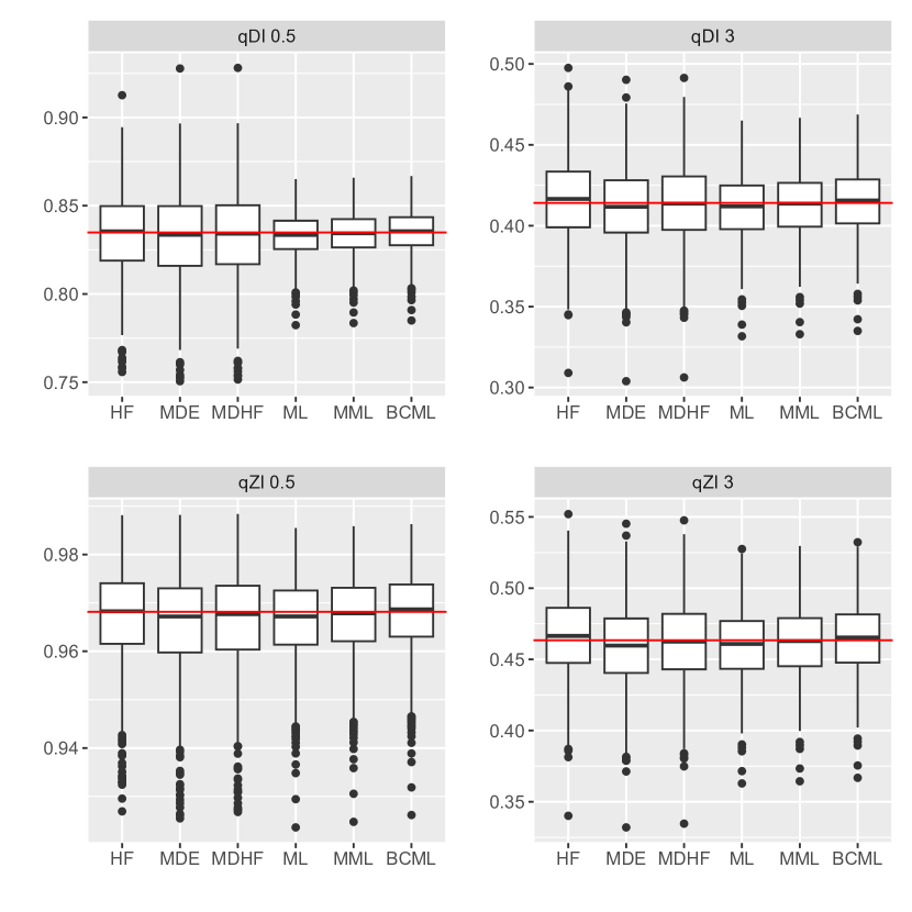
Figure 3. Boxplots depicting values of the estimators of $qDI$ (upper row) and $qZI$ (lower row) for sample of size $n=100$ from Weibull distribution with shape parameter $\beta=0.5$ (left column) and $\beta=3$ (right column) compared to the true value given with the red line

6. Real data analysis

We analyse here a data set containing numbers of days survived by guinea pigs infected with tubercle bacilli and a control group. These data appeared originally in [4] and were also considered by Doksum [11] and by Chandra and Singpurwalla [8]. According to the Anderson-Darling test (implemented in goftest package in R), there is no reason to reject the hypothesis that survival times of both groups have a Weibull distribution (with $p$ value $0.7381$ and $0.3702$, respectively). The test was performed for a null hypothesis that the distribution is Weibull with unknown parameters.

The values of the MML estimator of $\beta$ are $1.539$ for the control group and $2.201$ for the treated group. Figures 4 and 5 show the $qZ$ and $qD$ curves, respectively, for both groups constructed with the MML estimator (thick smooth lines) together with their empirical counterparts (thin step lines). The $x$ axis represents $p$  being an argument of $qZ$ or $qD$, and the values on the $y$ axis stand for the values of the concentration curves. A comparison of the estimators of the indices for both groups can be found in Table 5.

A Lorenz curve was applied by Chandra and Singpurwalla [8] to these data to compare the survival pattern of these two groups. The conclusion was that the infected group had a less sparse distribution of survival times. A similar conclusion can be drawn from the application of curves $qZ$ and $qD$. Both quantile concentration curves curves show that the control group has a significantly more sparse survival time. The empirical Lorenz curves cross near the point of $p=.8$ and on the interval $[0.8,1]$ they are almost equal. Empirical $qZ$ and $qD$ curves behave in a different way in the neighbourhood of 1; empirical $qZ$ curves also cross, but close to $p=.9$. Empirical $qD$ curves do not cross, but approach to each other on $[0.8,1]$. From this comparison we can see that each of this concentration curves show the differences in the survival pattern of the two groups in a different way, thus each of them might be useful to detect different types of inequalities in the populations.

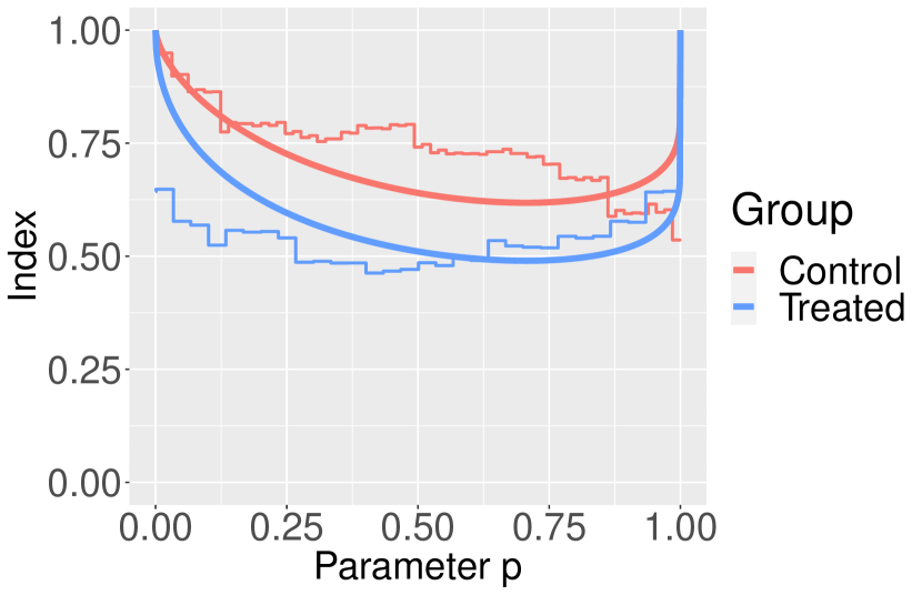
Figure 4. The $qZ$ of control group (red) and infected group (blue)

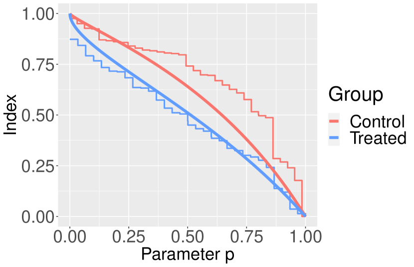
Figure 5. The $qD$ of control group (red) and infected group (blue)

Table 5. Estimates of the shape parameter, $qZI$ and $qDI$ obtained with MML estimator

	$\hat{\beta}^{MML}$	$\widehat{qZI}^{MML}$	$\widehat{qDI}^{MML}$
Control group	1.539	0.6941	0.5683
Treated group	2.201	0.5935	0.4968

7. Conclusions

In this article two novel parametric estimators of concentration curves $qZ$ and $qD$, based on the concept of minimum distance (MD) estimation, were introduced. They were compared to some other parametric estimators in case of Weibull distribution. It can be concluded that the class of MD estimators performs better than the nonparametric estimators, but worse than the plug-in estimators using several popular estimators of shape parameter. The experiment presented in Section 5 refers to the problem of estimating functions of parameters. In this particular case we could see that plug-in estimators based on standard estimators of the parameter give better estimators of the functions of parameters than estimators which are constructed directly to estimate that functions. This might be the case also in many similar problems when the object of estimation is a function of a parameter of a distribution of a random variable, not the parameter itself.

It can also be noticed that the MML estimator of the shape parameter of the Weibull distribution is slightly better than ML in all the cases considered in this paper. The BCML estimator of both indices has the lowest MSE for small values of $\beta$ (0.5, 1 and 2) and the MML has the lowest MSE for large values of $\beta$ (3). The advantage of MD estimators is their existence, thus they can be applied in cases when ML or other popular estimators might not exist or might be difficult to compute. Moreover, they may be recommended in the case when a good fit to the empirical concentration curve is desired. However, according to the simulation study, the curve matching to the empirical curve does not lead to the best estimation, comparing to the true curve.

Acknowledgement. The author would like to thank Alicja Jokiel-Rokita for careful reading of the manuscript and useful remarks and Rafał Topolnicki for valuable comments on the manuscript and on the simulation study.

8. Supplementary material

8.1. Introduction

In this supplementary material, the additional six methods are used to obtain plug-in estimators of $qZ$ and $qD$ curves and plug-in estimators of $qZI$ and $qDI$ indices. This methods use following estimators of the shape parameter $\beta$ of the Weibull distribution:

• Moment estimator (ME),

• L-moments estimator (LM),

• Tiku’s modified maximum likelihood estimator (TMML),

• Least squares estimator (LS),

• Weighted least squares estimator (WLS),

• Gini index-based estimator (G1).

Detailed description of ME, LM, TMML, LS and WLS can be found in [14], while G1 estimator is described in Section 3.2 in [20] as $\hat{\beta}_{\hat{G}}$. Moreover, an additional sample size 500 is considered and tables comparing bias of estimators of indices are included.

The estimators MML and BCML were chosen for a comparison in the main part of the work, since they were performing best (in terms of MSE and MISE) among the plug-in estimators. ML was added to the comparison because it is the state-of-the-art method used for estimation in variety of problems.

Analogously as in Section 5 of the main work, four values of the shape parameter $\beta$ were considered, namely $\beta\in\{0.5,1,2,3\}$. For each case, 10,000 samples were generated. Mean integrated square error (MISE) was used as a criterion to assess the estimators of the curves. The estimators of indices were compared in terms of MSE and bias.

8.2. Results of the extended simulation study

Twelve following tables contain comparison of performance of estimators of $qZ$, $qD$, $qZI$ and $qDI$. Tables 6, 7, 12 and 13 contain comparison of MSE of estimators. Tables 8, 9, 14 and 15 contain comparison of MISE of estimators. Tables 10, 11, 16 and 17 contain comparison of bias of estimators. Tables 6–11 contain comparison of estimators in case of sample sizes ($n$) 30 and 100, while 12–17 refer to the case when $n=500$.

Table 6. MSE (multiplied by 1,000) of the estimators of $qZI$ for sample sizes $n=30$ and $n=100$ and shape parameter varying between $0.5$ and $3$

	$30$				$100$
	0.5	1	2	3	0.5	1	2	3
HF	0.540	2.444	3.362	2.727	0.112	0.675	0.992	0.818
MDE	0.631	2.714	3.613	2.927	0.123	0.722	1.025	0.847
MDHF	0.544	2.466	3.408	2.805	0.117	0.694	0.998	0.827
ML	0.371	2.046	2.896	2.260	0.077	0.523	0.806	0.656
MML	0.318	1.866	2.742	2.203	0.073	0.500	0.787	0.650
BCML	0.270	1.753	2.725	2.257	0.070	0.489	0.786	0.656
ME	1.472	2.497	2.725	2.245	0.395	0.760	0.792	0.667
LM	0.513	2.007	2.839	2.384	0.136	0.563	0.823	0.703
TMML	0.367	2.022	2.865	2.264	0.078	0.517	0.799	0.656
LS	0.448	2.571	3.954	3.382	0.105	0.737	1.157	0.970
WLS	0.394	2.257	3.375	2.857	0.088	0.605	0.944	0.785
G1	0.776	2.372	3.023	2.449	0.159	0.598	0.839	0.708

Table 7. MSE (multiplied by 1,000) of the estimators of $qDI$ for sample sizes $n=30$ and $n=100$ and shape parameter varying between $0.5$ and $3$

	$30$				$100$
	0.5	1	2	3	0.5	1	2	3
HF	2.108	2.687	2.643	2.113	0.617	0.828	0.798	0.642
MDE	2.522	2.981	2.662	2.060	0.741	0.895	0.780	0.607
MDHF	2.389	2.856	2.559	1.996	0.728	0.886	0.767	0.598
ML	0.596	1.319	1.748	1.478	0.150	0.346	0.481	0.425
MML	0.544	1.219	1.647	1.431	0.146	0.330	0.469	0.420
BCML	0.509	1.171	1.628	1.452	0.143	0.326	0.468	0.423
ME	1.905	1.612	1.636	1.458	0.638	0.502	0.472	0.431
LM	0.865	1.329	1.701	1.543	0.267	0.374	0.490	0.454
TMML	0.594	1.304	1.727	1.479	0.150	0.340	0.477	0.425
LS	0.788	1.726	2.366	2.175	0.213	0.491	0.688	0.625
WLS	0.681	1.499	2.022	1.845	0.175	0.401	0.562	0.507
G1	1.106	1.516	1.825	1.605	0.288	0.392	0.501	0.459

Table 8. MISE (multiplied by 1,000) of the estimators of $qZ$ for sample sizes $n=30$ and $n=100$ and shape parameter varying between $0.5$ and $3$

	$30$				$100$
	0.5	1	2	3	0.5	1	2	3
HF	0.861	4.399	7.155	6.705	0.215	1.358	2.204	2.086
MDE	0.735	2.851	3.633	2.946	0.147	0.764	1.031	0.852
MDHF	0.635	2.596	3.429	2.822	0.140	0.735	1.005	0.832
ML	0.435	2.152	2.912	2.274	0.093	0.554	0.811	0.659
MML	0.375	1.968	2.759	2.216	0.088	0.530	0.792	0.654
BCML	0.321	1.857	2.745	2.268	0.084	0.519	0.791	0.660
ME	1.696	2.625	2.742	2.259	0.465	0.805	0.797	0.670
LM	0.603	2.122	2.858	2.397	0.162	0.597	0.828	0.707
TMML	0.431	2.127	2.881	2.278	0.093	0.547	0.804	0.659
LS	0.526	2.722	3.985	3.400	0.126	0.782	1.164	0.975
WLS	0.463	2.386	3.399	2.873	0.106	0.642	0.950	0.789
G1	0.901	2.490	3.040	2.465	0.189	0.633	0.844	0.712

Table 9. MISE (multiplied by 1,000) of the estimators of $qD$ for sample sizes $n=30$ and $n=100$ and shape parameter varying between $0.5$ and $3$

	$30$				$100$
	0.5	1	2	3	0.5	1	2	3
HF	5.914	5.483	4.834	4.261	2.033	1.853	1.534	1.320
MDE	4.192	3.675	3.018	2.408	1.286	1.108	0.882	0.707
MDHF	4.037	3.546	2.900	2.325	1.269	1.099	0.867	0.696
ML	0.989	1.604	1.982	1.732	0.259	0.428	0.544	0.495
MML	0.918	1.492	1.865	1.671	0.253	0.408	0.530	0.489
BCML	0.880	1.450	1.843	1.688	0.251	0.404	0.529	0.492
ME	2.960	1.960	1.853	1.703	1.057	0.619	0.533	0.502
LM	1.463	1.637	1.926	1.798	0.463	0.463	0.554	0.528
TMML	0.986	1.585	1.957	1.732	0.260	0.419	0.539	0.495
LS	1.349	2.138	2.680	2.527	0.372	0.609	0.778	0.726
WLS	1.158	1.848	2.291	2.148	0.305	0.496	0.635	0.590
G1	1.774	1.833	2.069	1.883	0.490	0.482	0.566	0.535

Table 10. Bias (multiplied by 1,000) of the estimators of $qZ$ for sample sizes $n=30$ and $n=100$ and shape parameter varying between $0.5$ and $3$

	$30$				$100$
	0.5	1	2	3	0.5	1	2	3
HF	-8.562	-12.138	-9.065	-5.756	-2.458	-3.766	-2.198	-1.177
MDE	-9.912	-15.680	-14.410	-11.931	-2.860	-5.160	-4.407	-3.776
MDHF	-7.702	-10.462	-7.921	-5.786	-2.297	-3.372	-1.893	-1.104
ML	-6.843	-12.915	-13.290	-10.044	-1.845	-3.995	-3.717	-2.727
MML	-4.488	-6.967	-6.030	-3.370	-1.191	-2.309	-1.576	-0.765
BCML	-1.685	0.399	3.108	5.060	-0.381	-0.109	1.151	1.746
ME	-26.454	-16.530	-6.218	-3.018	-11.053	-5.759	-1.701	-0.651
LM	-6.675	-3.970	-1.516	-0.037	-2.103	-1.490	-0.280	0.157
TMML	-6.666	-12.448	-12.722	-9.500	-1.867	-4.119	-3.788	-2.831
LS	-2.259	1.557	6.387	8.042	-0.583	0.249	1.913	2.448
WLS	-2.888	-1.235	2.029	3.867	-0.994	-1.385	-0.129	0.371
G1	-14.936	-17.861	-15.634	-12.233	-4.420	-5.615	-4.505	-3.494

Table 11. Bias (multiplied by 1,000) of the estimators of $qD$ for sample sizes $n=30$ and $n=100$ and shape parameter varying between $0.5$ and $3$

	$30$				$100$
	0.5	1	2	3	0.5	1	2	3
HF	-10.529	-7.425	-4.419	-2.799	-3.091	-2.642	-1.246	-0.595
MDE	-12.732	-9.318	-7.384	-6.731	-3.341	-3.150	-2.264	-2.069
MDHF	-9.495	-5.470	-2.367	-1.438	-2.609	-2.045	-0.715	-0.178
ML	-7.141	-9.750	-10.483	-8.415	-1.936	-3.024	-2.926	-2.289
MML	-3.911	-4.918	-4.867	-3.040	-1.000	-1.661	-1.275	-0.712
BCML	0.062	1.121	2.196	3.731	0.172	0.135	0.829	1.304
ME	-30.234	-12.525	-5.010	-2.763	-13.061	-4.363	-1.372	-0.623
LM	-5.582	-2.366	-1.385	-0.387	-1.726	-0.960	-0.278	0.020
TMML	-6.890	-9.378	-10.048	-7.978	-1.967	-3.134	-2.982	-2.373
LS	0.521	2.444	4.645	5.964	0.226	0.542	1.389	1.822
WLS	-0.922	-0.020	1.313	2.682	-0.565	-0.858	-0.171	0.180
G1	-16.736	-13.705	-12.311	-10.204	-5.020	-4.323	-3.538	-2.914

Table 12. MSE (multiplied by 10,000) of the estimators of $qZI$ for sample size $n=500$ and shape parameter varying between $0.5$ and $3$

	0.5	1	2	3
HF	0.1938	1.3409	1.9393	1.6931
MDE	0.2093	1.3938	1.9611	1.7199
MDHF	0.2066	1.3825	1.9509	1.7059
ML	0.1332	1.0089	1.5247	1.3087
MML	0.1309	1.0046	1.5210	1.3027
BCML	0.1293	1.0027	1.5217	1.3029
ME	0.8594	1.5746	1.5514	1.3461
LM	0.2509	1.1305	1.5972	1.4212
TMML	0.1330	1.0111	1.5268	1.3075
LS	0.1991	1.4873	2.2497	1.9713
WLS	0.1583	1.1866	1.7861	1.5540
G1	0.2606	1.1380	1.6014	1.4253

Table 13. MSE (multiplied by 10,000) of the estimators of $qDI$ for sample size $n=500$ and shape parameter varying between $0.5$ and $3$

	0.5	1	2	3
HF	1.2272	1.6897	1.5778	1.3406
MDE	1.4756	1.8180	1.5194	1.2435
MDHF	1.4680	1.8162	1.5159	1.2372
ML	0.2774	0.6698	0.9067	0.8453
MML	0.2737	0.6677	0.9043	0.8411
BCML	0.2725	0.6674	0.9044	0.8408
ME	1.7127	1.0462	0.9223	0.8691
LM	0.5233	0.7521	0.9494	0.9173
TMML	0.2764	0.6711	0.9080	0.8447
LS	0.4179	0.9904	1.3371	1.2714
WLS	0.3306	0.7887	1.0618	1.0031
G1	0.5332	0.7551	0.9524	0.9207

Table 14. MISE (multiplied by 10,000) of the estimators of $qZ$ for sample size $n=500$ and shape parameter varying between $0.5$ and $3$

	0.5	1	2	3
HF	0.4028	2.7817	4.4926	4.2785
MDE	0.2526	1.4802	1.9732	1.7284
MDHF	0.2495	1.4686	1.9631	1.7143
ML	0.1609	1.0716	1.5340	1.3152
MML	0.1582	1.0673	1.5305	1.3091
BCML	0.1564	1.0656	1.5312	1.3093
ME	1.0323	1.6726	1.5610	1.3527
LM	0.3030	1.2013	1.6072	1.4282
TMML	0.1607	1.0740	1.5361	1.3140
LS	0.2407	1.5807	2.2639	1.9809
WLS	0.1913	1.2607	1.7972	1.5616
G1	0.3143	1.2086	1.6113	1.4324

Table 15. MISE (multiplied by 10,000) of the estimators of $qD$ for sample size $n=500$ and shape parameter varying between $0.5$ and $3$

	0.5	1	2	3
HF	4.2987	3.8925	3.1423	2.7204
MDE	2.5884	2.2570	1.7164	1.4467
MDHF	2.5746	2.2554	1.7124	1.4390
ML	0.4858	0.8303	1.0242	0.9837
MML	0.4798	0.8282	1.0214	0.9786
BCML	0.4783	0.8285	1.0215	0.9779
ME	2.9800	1.2975	1.0418	1.0111
LM	0.9171	0.9334	1.0724	1.0671
TMML	0.4838	0.8319	1.0256	0.9830
LS	0.7334	1.2295	1.5103	1.4784
WLS	0.5794	0.9783	1.1994	1.1668
G1	0.9305	0.9358	1.0758	1.0714

Table 16. Bias (multiplied by 1,000) of the estimators of $qZI$ for sample size $n=500$ and shape parameter varying between $0.5$ and $3$

	0.5	1	2	3
HF	-0.488	-0.431	-0.159	-0.250
MDE	-0.577	-0.751	-0.747	-1.017
MDHF	-0.457	-0.363	-0.130	-0.297
ML	-0.393	-0.517	-0.668	-0.752
MML	-0.269	-0.170	-0.239	-0.370
BCML	-0.109	0.269	0.306	0.130
ME	-3.307	-0.790	-0.254	-0.314
LM	-0.498	0.100	0.065	-0.122
TMML	-0.422	-0.582	-0.747	-0.835
LS	-0.107	0.369	0.607	0.428
WLS	-0.260	-0.099	-0.049	-0.192
G1	-0.950	-0.721	-0.779	-0.851

Table 17. Bias (multiplied by 1,000) of the estimators of $qDI$ for sample size $n=500$ and shape parameter varying between $0.5$ and $3$

	0.5	1	2	3
HF	-0.649	-0.221	0.016	-0.129
MDE	-0.563	-0.250	-0.202	-0.549
MDHF	-0.619	-0.116	0.108	-0.095
ML	-0.432	-0.375	-0.526	-0.624
MML	-0.253	-0.092	-0.195	-0.317
BCML	-0.019	0.266	0.225	0.085
ME	-3.954	-0.571	-0.207	-0.272
LM	-0.458	0.134	0.038	-0.119
TMML	-0.475	-0.428	-0.587	-0.690
LS	0.057	0.370	0.451	0.314
WLS	-0.210	-0.026	-0.051	-0.178
G1	-1.113	-0.536	-0.613	-0.705

8.3. Conclusions

The methods which were not included in the main article perform worse than BCML and MML in all cases considered. The TMML method gives results close to ML, since it is an approximation of ML. In terms of bias it seems that the BCML is best for small $\beta$ (0.5 and 1), while LM is best in case of larger $\beta$ (2 and 3). The simulations performed for larger sample size (500) give similar conclusions as the ones with smaller sample sizes (30 and 100), but in this case MML is slightly better than BCML in terms of MSE and MISE when $\beta$ is 1 and 2.

References

- [1] Al-Deek, H., and Emam, E. B. New methodology for estimating reliability in transportation networks with degraded link capacities. Journal of Intelligent Transportation Systems 10, 3 (2006), 117–129.
- [2] Bandourian, R., McDonald, J., and Turley, R. A comparison of parametric models of income distribution across countries and over time. SSRN Electronic Journal 55 (2002).
- [3] Basu, A., Shioya, H., and Park, C. Statistical Inference The Minimum Distance Approach (1st ed.). Chapman and Hall/CRC, 2011.
- [4] Bjerkedal, T. Acquisition of resistance in guinea pigs infected with different doses of virulent tubercle bacilli. American Journal of Epidemiology 72, 1 (1960), 130–148.
- [5] Bonferroni, C. E. Elementi di Statisica Generale. Firenze:Libreria Seeber, 1930.
- [6] Brazauskas, V., Greselin, F., and Zitikis, R. Measuring income inequality via percentile relativities. https://arxiv.org/abs/2308.03708, 2023.
- [7] Chakraborti, A., Fujiwara, Y., Ghosh, A., Inoue, J.-i., and Sinha, S. Physicists’ Approaches to a Few Economic Problems. Springer International Publishing, 2015, pp. 237–286.
- [8] Chandra, M., and Singpurwalla, N. D. Relationships between some notions which are common to reliability theory and economics. Math. Oper. Res. 6 (1981), 113–121.
- [9] Davidov, O., and Nov, Y. Minimum-norm estimation for binormal receiver operating characteristic (ROC) curves. Biometrical journal. Biometrische Zeitschrift 51 (2009), 1030–46.
- [10] Davydov, Y., and Greselin, F. Comparisons between poorest and richest to measure inequalty. Sociological Methods Research 49, 2 (2020), 526–561.
- [11] Doksum, K. Empirical Probability Plots and Statistical Inference for Nonlinear Models in the Two-Sample Case. The Annals of Statistics 2, 2 (1974), 267 – 277.
- [12] Duan, W., Shan, Z., Christidis, N., Schaller, N., Yaning, C., Sahu, N., Li, Z., Fang, G., and Zhou, B. Changes in temporal inequality of precipitation extremes over China due to anthropogenic forcings. npj Climate and Atmospheric Science 5 (2022), 33.
- [13] Fan, Z. Minimum-distance estimator for stable exponent. Communications in Statistics - Theory and Methods 38, 4 (2009), 511–528.
- [14] Gebizlioglu, O. L., Şenoğlu, B., and Kantar, Y. M. Comparison of certain value-at-risk estimation methods for the two-parameter Weibull loss distribution. Journal of Computational and Applied Mathematics 235, 11 (2011), 3304–3314.
- [15] Gneiting, T., and Vogel, P. Receiver operating characteristic (ROC) curves: equivalences, beta model, and minimum distance estimation. Machine Learning 111 (2022).
- [16] Hopfner, R., and Rueschendorf, L. Comparison of estimators in stable models. Mathematical and Computer Modelling 29 (1999).
- [17] Hsieh, F., and Turnbull, B. W. Nonparametric and semiparametric estimation of the receiver operating characteristic curve. The Annals of Statistics 24, 1 (1996), 25 – 40.
- [18] Hyndman, R. J., and Fan, Y. Sample quantiles in statistical packages. The American Statistician 50, 4 (1996), 361–365.
- [19] Jin, H., Chen, X., Ruida, Z., Pan, Y., Zhao, T., Liu, Z., and Tu, X. Spatiotemporal distribution analysis of extreme precipitation in the Huaihe River Basin based on continuity. Natural Hazards 114 (2022), 1–30.
- [20] Jokiel-Rokita, A., and Piątek, S. Estimation of parameters and quantiles of the Weibull distribution. Statistical Papers (2022).
- [21] Jokiel-Rokita, A., and Piątek, S. Nonparametric estimators of inequality curves and inequality measures. https://arxiv.org/abs/2310.16200, 2023.
- [22] Jokiel-Rokita, A., and Topolnicki, R. Minimum distance estimation of the binormal ROC curve. Statistical Papers 60 (2019), 1–23.
- [23] Jokiel-Rokita, A., and Topolnicki, R. Minimum distance estimation of the Lehmann receiver operating characteristic curve. Statistics 55, 3 (2021), 618–634.
- [24] Kim, H.-M., Jang, Y.-H., Arnold, B., and Zhao, J. New efficient estimators for the Weibull distribution. Communications in Statistics - Theory and Methods (2023), 1–26.
- [25] Lee, S.-B., Lee, S. M., and Lee, K.-Y. A Gini coefficient based evaluation on the reliability of travel time forecasting. Journal of King Saud University - Engineering Sciences 31, 4 (2019), 314–319.
- [26] Lorenz, M. O. Methods of measuring the concentration of wealth. Publications of the American Statistical association 9, 70 (1905), 209–219.
- [27] Makalic, E., and Schmidt, D. Maximum likelihood estimation of the Weibull distribution with reduced bias. Statistics and Computing 33 (2023).
- [28] Millar, P. W. A general approach to the optimality of minimum distance estimators. Transactions of the American Mathematical Society 286 (1984), 377–418.
- [29] Prendergast, L. A., and Staudte, R. G. Quantile versions of the Lorenz curve. Electronic Journal of Statistics 10 (2016), 1896–1926.
- [30] Prendergast, L. A., and Staudte, R. G. A simple and effective inequality measure. The American Statistician 72, 4 (2018), 328–343.
- [31] Sazuka, N., and ichi Inoue, J. Fluctuations in time intervals of financial data from the view point of the Gini index. Physica A: Statistical Mechanics and its Applications 383, 1 (2007), 49–53.
- [32] Seki, T., and Yokoyama, S. Simple and robust estimation of the Weibull parameters. Microelectronics Reliability 33, 1 (1993), 45–52.
- [33] Shen, Y., and Yang, Z. Bias-correction for Weibull common shape estimation. Journal of Statistical Computation and Simulation (2014).
- [34] Siedlaczek, A. Nonparametric estimation of quantile versions of the Lorenz curve. Mathematica Applicanda 46 (2018).
- [35] Teimouri, M., Hoseini, S., and Nadarajah, S. Comparison of estimation methods for the Weibull distribution. Statistics (2011).
- [36] van der Vaart, A. W. Asymptotic Statistics. Cambridge Series in Statistical and Probabilistic Mathematics. Cambridge University Press, 1998.
- [37] Weibull, W. The phenomenon of rupture in solids. Ingeniors Vetenskaps Akademien Handlingar 153 (1939), 17.
- [38] Wolfowitz, J. The Minimum Distance Method. The Annals of Mathematical Statistics 28, 1 (1957), 75 – 88.
- [39] Yang, X., Xie, L., Yang, Y., Zhao, B., and Li, Y. A comparative study for parameter estimation of the Weibull distribution in a small sample size: An application to spring fatigue failure data. Quality Engineering 35, 4 (2023), 553–565.
- [40] Zenga, M. Inequality curve and inequality index based on the ratios between lower and upper arithmetic means. Statistica Applicazioni 5, 1 (2007), 3–27.